Mode-coupling theory and molecular dynamics simulation …polymer.chph.ras.ru/asavin/teplopr/wl04pre.pdf · Mode-coupling theory and molecular dynamics simulation for heat conduction

Mode-coupling theory and molecular dynamics simulation for heat conduction in a chainwith transverse motions

Jian-Sheng WangSingapore-MIT Alliance and Department of Computational Science, National University of Singapore,

Singapore 117543, Republic of Singapore

Baowen LiDepartment of Physics, National University of Singapore, Singapore 117542, Republic of Singapore

(Received 5 March 2004; published 19 August 2004)

We study heat conduction in a 1D chain of particles with longitudinal as well as transverse motions. Theparticles are connected by 2D harmonic springs together with bending angle interactions. The problem isanalyzed by mode-coupling theory and compared with molecular dynamics. We find very good, quantitativeagreement for the damping of modes between a full mode-coupling theory and molecular dynamics result, anda simplified mode-coupling theory gives qualitative description of the damping. The theories predict generi-cally that thermal conductance diverges asN1/3 as the sizeN increases for systems terminated with heat bathsat the ends. TheN2/5 dependence is also observed in molecular dynamics, which we attribute to crossovereffect.

DOI: 10.1103/PhysRevE.70.021204 PACS number(s): 44.10.1i, 05.70.Ln, 05.45.2a, 66.70.1f

I. INTRODUCTION

The problem of heat conduction is a well-studied field.More than two centuries ago, Joseph Fourier summarized thebehavior of heat conduction by the law that bears his name.This law describes phenomenologically that the heat currentis proportional to the temperature gradient. The detailed ato-mistic theories of heat conduction appeared only much later.For heat conduction in gas, the simple kinetic theory gives

the resultk= 13Cvl, whereC is specific heat,v is average

velocity, andl is mean-free path. Peierls’ theory of heat con-duction in insulating solids[1] is a classic on this subject.These early theories deal with mostly the relevant three di-mensions. It turns out that low-dimensional systems are moreinteresting and in some sense strange. An analysis of asimple one-dimensional(1D) harmonic oscillator modelshows[2] that there is no well-defined temperature gradient,the thermal conductivity diverges with system sizes asN1/2

or N, depending on the boundary conditions. There is a gen-eral argument, for momentum conserving systems, that thethermal conduction in 1D is necessarily divergent[3].

There have been many analytical and numerical studies of1D heat conduction(see Refs.[4,5] for review). We mentionsome of the most relevant papers to current work. The workof Lepri, Livi, and Politi [6] by mode-coupling theory andmolecular dynamics suggests a divergent thermal conductiv-ity exponent of 2/5, i.e.,k~N2/5 for a 1D chain model withFermi-Pasta-Ulam(FPU) interactions. Mode-coupling theoryis usually applied in the dynamics of liquids[7,8]. The firstuse of this theory in the context of heat conduction appearsonly recently, mostly due to Lepri and his collaborators[9].Pereverzev analyzed the same problem with the Peierlstheory for phonon gas and gave the same conclusion of 2/5exponent[10]. The result of 2/5 is also supported by numeri-cal simulation from several groups[11–14]. These results aresupposed to be universal to some extent. However, it is chal-

lenged by a different result of 1/3 by Narayan and Ra-maswamy [15], based on fluctuating hydrodynamics andrenormalization group analysis. The numerical result for this1/3 law is not convincing, as for the same model—the hard-particle gas model—some obtained 1/3[16,17], while othersobtained different value 1/4[18]. But for the FPU model,there is no good evidence for an exponent of 1/3[19].

When momentum conservation is broken, such as the onewith on-site potential, the heat conduction can become nor-mal again like the Frenkel-Kontorova model[20] and thef4

model [14,21].In order to understand the underlying microscopic dy-

namical mechanism of the Fourier law, a different class ofmodels—billiard channels—has been introduced and studiedin recent years[22,23]. Various exponent values are found insuch systems. Thus, it is believed that a universal constantdoes not exist at all. Instead, the divergent(convergent) ex-ponent of the thermal conductivity is found related to thepower of super(sub) diffusion [23].

Besides the theoretical significance of heat conduction re-search in low-dimensional systems, it is also of practical im-portance. Recent development of nanotechnology will enableus to manufacture devices with feature sizes at molecularlevel. The understanding of the heat conduction mechanismwill allow us to control and manipulate heat current, andeventually to design novel thermal devices with certain func-tion [24]. To this end, more realistic physical models arenecessary. Among many others, nanotubes and polymerchains are most promising. There have been a number ofnumerical works to compute the thermal conductivity of theCarbon nanotubes[25,26]. Recent molecular dynamics(MD)study of carbon nanotubes with realistic interaction potentialsuggested a divergent thermal conductivity for narrow diam-eter tubes[27,28]. The quantum effect of such systems isalso very interesting[29,30].

We study the heat conduction of a 1D solid, as a classicalsystem. A brief version of this paper is reported in Ref.[31].

PHYSICAL REVIEW E 70, 021204(2004)

1539-3755/2004/70(2)/021204(16)/$22.50 ©2004 The American Physical Society70 021204-1

In the rest of the paper, we introduce the quasi-1D chainmodel in Sec. II. We discuss the basis of the mode-couplingtheory, the projection method in Sec. III. The mode-couplingapproximations and their numerical and analytical solutionsare discussed in Secs. IV and V. The basic output of themode-coupling analysis is the dependence of damping of themodes with the wave vector of the modes. We find that thetransverse modes are diffusive, withgp

'~p2, while the lon-gitudinal modes are superdiffusive,gp

i~p3/2, wheregp is the

decay rate for mode with momentum or lattice wave numberp. We discuss the relationship between the damping of themodes with the heat conductivity through the Green-Kuboformula in Sec. VI. Our mode-coupling theory predicts thatthe heat conductance diverges with the 1/3 exponent whenthe transverse motions are important, while 2/5 is recoveredif the transverse motions can be neglected. In Sec. VII, wepresent nonequilibrium molecular dynamics results(withheat baths) of heat conductance and compare with mode-coupling theory. We conclude in the last section.

II. CHAIN MODEL

Most of the previous studies considered only strictly 1Dmodels, with the FPU model as the most representative. Thestrictly 1D models may not be applicable to real systems,such as the nanotubes. Real systems of nanotubes or wireslive in 3D space. The added transverse motion and the flex-ibility of the tube at long length scales will certainly scatterphonons, and thus should have a profound effect on thermaltransport.

While a direct simulation of a realistic system, such as apolyethelene chain with empirical force fields(as in Refs.[32,33]), or a nanotube with Tersoff potential[34] is pos-sible, we think it is useful to consider a simplified modelwhich captures one of the important features of the realsystems—transverse degrees of freedom. Therefore we pro-pose to study the following chain model in 2D[31]:

Hsp,r d = oi

pi2

2m+

1

2Kro

i

sur i+1 − r iu − ad2 + Kfoi

cosfi ,

s1d

where the position vectorr =sx,yd and momentum vectorp=spx,pyd are 2D;a is lattice constant. The minimum energystate is atsia ,0d for i =0 toN−1. If the system is restricted toyi =0 (corresponding toKf= +`), it is essentially a 1D gaswith harmonic interaction. The couplingKr is the spring con-stant;Kf signifies bending or flexibility of the chain, whilefi is the bond angle formed with two neighboring sites,cosfi =−ni−1·ni, and unit vectorni =Dr i / uDr iu, Dr i =r i+1−r i.

Unlike the FPU model, which does not have an energyscale, the second bond-angle bending term introduces an en-ergy scale. In this work, we take massm=1, spring constantKr =1, and the Boltzmann constantkB=1, thus the most im-portant parameters areKf and temperatureT.

III. PROJECTION METHOD

A. Basic theory of projection

We follow the formulation of the projection method inRef. [35]. Let

A =1a1

a2

Aan

2 s2d

be a column vector ofn components of some arbitrary func-tions of dynamical variablessp,qd. Each of the functionsajsp,qd can be complex. Later, we shall chooseaj to be thecanonical coordinates of the system. We useA†

=sa1* ,a2

* ,¯ ,an*d to denote the Hermitian conjugate ofA. The

equation of motion forA is

At = LAt, or ajstd = Lajstd, s3d

whereL is the Liouville operator

L = − o ] H

] q

]

] p+ o ] H

] p

]

] q. s4d

Equation(3) can be viewed as a partial differential equationwith variablessp,qd and timet. At;Aspt ,qtd=Ast ,p,qd, i.e.,the quantityA at time t when the initial condition att=0 issp,qd. Quantity without a subscriptt will be understood to beevaluated at timet=0, e.g.,p=pt=0=ps0d. A formal solutionto Eq. (3) is simply At=etLAsp,qd. The projection operatoron a column vectorX is defined by

PX = kX,A†lkA,A†l−1A, s5d

where kX,A†l and kA,A†l are n3n matrices. The angularbrackets denote the thermodynamical average in a canonicalensemble at temperatureT. The comma separating the twoterms is immaterial, but we use a notation of inner product.One can verify thatP is indeed a projection operator, i.e.,P2=P.

If we apply the projection operatorP andP8=1−P to theequation of motion, we get two coupled equations. Solvingformally the second equation associated withP8 and substi-tuting it back into the first equation, we obtain an equationfor the projected variable that formally resembles a Langevinequation:

At = iVAt −E0

t

Gst − sdAs ds+ Rt, s6d

wherei =Î−1 is the complex unit, and

Gstd = kRt,R0†lkA,A†l−1, s7d

iV = kA,A†lkA,A†l−1, s8d

Rt = etP8LR0, R0 = A − iVA = P8LA. s9d

This set of equations is deterministic and formally exact. Theonly assumption made is that equilibrium distribution can be

J.-S. WANG AND B. LI PHYSICAL REVIEW E70, 021204(2004)

021204-2

realized. What is more important is the correlation functions,which are physical observables. We define the normalizedcorrelation function(correlation matrix) as

Gstd = kAt,A0†lkA,A†l−1. s10d

It is an identity matrix att=0 and has the property that

Gs0d= iV. From Eq.(6) we have,

Gstd = iVGstd −E0

t

Gst − sdGssdds. s11d

This equation can be solved formally using proper initialcondition with a Fourier-Laplace transform,

Gfzg =E0

`

e−iztGstddt, s12d

and similarly forGstd. The solution is

Gfzg = sisz− Vd + Gfzgd−1. s13d

To simplify notation, we have used parentheses[e.g.,Gstd]for functions in time domain, and square brackets with thesame symbol(e.g., Gfzg) for their corresponding Fourier-Laplace transform in frequency domain.

The information about the system is in the memory kernelGstd. However, such a correlation function is difficult to cal-culate, since the evolution of the “random force”Rt does notfollow the dynamics of the original Hamiltonian system. Forexample, it is impossible to compute directlyRt from mo-lecular dynamics. For this reason, a “true force” can be in-troduced which obeys the normal evolution, i.e.,

Ft = etLR0 = At − iVAt. s14d

The correlation function of the true force,

GFstd = kFt,F0†lkA,A†l−1, s15d

and that of the random force are related in Fourier space as[35]

Gfzg−1 = GFfzg−1 − fisz− Vdg−1. s16d

This completes the formal theory of projection due originallyto Zwanzig[36] and Mori [37]. These results are formal andexact. They give us relation between correlation of the“force” and correlation of dynamical variables. They are thestarting point for mode-coupling theory. In the next subsec-tions, we apply it to our chain model and introduce a seriesof approximations to solve it.

B. The chain model

We now apply the projection method to our chain model.We choose the normal modes as the basic quantitiesaj thatwe are going to project out. There are several reasons forchoosing the normal modes. To zeroth order approximation,each mode is nearly independent. The slowest process corre-sponds to long wave-length modes. The effect of short wave-length modes can be treated as stochastic noise(the randomforce Rt).

We chooseA to be the complete set of canonical momentaand coordinates:

A =1Pk

i

Pk'

Qki

Qk'2, k = 0,1,¯ ,N − 1, s17d

where

Qki =Îm

Noj=0

N−1

ujei2p jk/N, s18d

Qk' =Îm

Noj=0

N−1

yjei2p jk/N, s19d

Pki = Qk

i =1

ÎmNoj=0

N−1

pj ,xei2p jk/N, s20d

Pk' = Qk

' =1

ÎmNoj=0

N−1

pj ,yei2p jk/N. s21d

We have defined the position vectorr j =sxj ,yjd=suj +aj ,yjd,so thatuj andyj are deviations from zero-temperature equi-librium position. Because the Fourier transform is a periodicfunction, the indexk is unique only moduloN. As a result,we can also letk vary in the range −N/2øk,N/2. We alsonote thatQk

* =Q−k.With these definitions, we can compute the matrixV and

expression for the true forceF in the general theory. We findthat for kA,A†l, the components are

kPkmPk8

n*l = dkk8dmn

1

b, m,n = i , ' , s22d

kPkmQk8

n*l = 0, s23d

kQkmQk8

n*l = dkk8dmn

1

bsvkmd2, b =

1

kBT. s24d

We have used equal-partition theorem for the average kineticenergy expression, and the last equation merely defines theeffective frequenciesvk

m for each mode. Note that due totranslational invariance, correlation between differentkmodes vanishes. Correlation between transverse and longitu-dinal modes also vanishes due to the reflection symmetry ofyj →−yj for the chain. Thus equal-time correlation forA isdiagonal,

kA,A†l =1

bS I 0

0 v−2D . s25d

We have definedv as a 2N32N diagonal matrix with ele-mentsvk

m; I is a 2N32N identity matrix. Similarly, the cor-

relation kA,A†l is found from

kPkmPk8

n*l = 0, s26d

MODE-COUPLING THEORY AND MOLECULAR DYNAMICS… PHYSICAL REVIEW E 70, 021204(2004)

021204-3

kPkmQk8

n*l = − dkk8dmn

1

b, s27d

kQkmPk8

n*l = dkk8dmn

1

b, s28d

kQkmQk8

n*l = 0. s29d

The second equation is from a general virial theorem[38].We have

iV = kA,A†lkA,A†l−1 = S0 − v2

I 0D . s30d

The expression for the true forceF=A− iVA is then

F ; SFP

FQD = SPkm + vk

m2Qkm

0D . s31d

Note that only the momentum sector has a nonzero value,

and Pkm=Qk

m is given approximately by Eqs.(50) and (51).With this special form ofF, the damping matrixG is alsodiagonal and is nonzero only in thePP components. Withthese results, Eq.(13) becomes

Gfzg = Sizd − v2d

d siz + GfzgddD , s32d

whered=sv2−z2I + izGfzgd−1 is a 2N32N diagonal matrix,

and Gfzg is the Fourier-Laplace transform of the correlationbkRt

P,sRPd†l, which is also diagonal[we’ll denote asGkmstd].

In particular, we have the usual expression for the normal-ized coordinate correlation,

gQQ,km std =

kQkmstdQ−k

m s0dlkuQk

mu2l, s33d

gQQ,km fzg =

iz + Gkmfzg

vkm2 − z2 + izGk

mfzg. s34d

For simplicity, we drop theQQ subscript for the coordinatecorrelation for the rest of the paper. Finally, the relation be-tween the random force correlation and true force correla-tion, Eq. (16), becomes,

1

Gkmfzg

=1

GF,km fzg

−iz

vkm2 − z2 . s35d

The force correlationGF,km can be computed from the corre-

lation functionbkFtP,sFPd†l. It is convenient to separate the

linear term in the force from the nonlinear contribution. Sowe write

FPstd = v2Qstd + Qstd = sv2 − v02dQstd + fNstd, s36d

wherev is effective angular frequency andv0 is bare angu-lar frequency of the mode. We have dropped the indiceskandm because these equations apply for any of the modes.fNis at least quadratic inQ. We note that the correlation of

FPstd is linearly related to the coordinate correlation functiongfzg,

GFfzg =− izsv2 − z2d

v2 +sv2 − z2d2

v2 gfzg. s37d

This is simply a consequence of Eqs.(34) and (35), but canalso be derived directly from the definition. The second de-rivative of Qstd in frequency domain isQfzg multiplied bysizd2. Using the fact that

lime→0+

E0

`

Qstde−izt−etdt = − z2Qfzg − Qs0d − izQs0d, s38d

we can also derive Eq.(37) with the understanding thatk¯lis an average over the initial conditions. Sincegfzg is finiteor at least should not diverge precisely atz=v, this impliesGFfvg=0. With the above results, we can derive an expres-sion of the true force correlation in terms of nonlinear forcecorrelation,

GFstdb

= kFPstdFPs0d*l=Dv4kQstdQ*s0dl + kfNstdfNs0d*l

− Dv2skfNstdQ*s0dl + kQstdfN* s0dld, s39d

where Dv2=v02−v2. The mixed term can be expressed in

terms of gfzg by noting that fN=Q+v02Q. The two mixed

terms kfNstdQ*s0dl and kQstdfN* s0dl are equal due to time-

reversal symmetry. We find

bv2E0

`

kfNstdQ*s0dle−iztdt = sv02 − z2dgfzg − iz. s40d

Finally, we have

GFfzg =Dv2

v2 ss2z2 − v02 − v2dgfzg + 2izd + GNfzg. s41d

We can also expressgfzg in terms of the nonlinear part of theforce correlation,GNs=bkfNstdfNs0d*ld:

gfzg =izs2v0

2 − v2 − z2d + v2GNfzgsz2 − v0

2d2 . s42d

Again, sincegfzg cannot diverge precisely atz=v0, this im-plies thatGNfzg must take a special form to cancel the appar-ent divergence. Thus, if we do not take care of these super-ficial divergences, we will not be able to make correctprediction for the correlation function. We can also relate theoriginal damping functionG to the nonlinear one,

Gfzg =− isv2 − v0

2d2z+ v2sv2 − z2dGNfzgv0

4 − v2z2 − izv2GNfzg. s43d

This last equation is useful for approximating the dampingfunction. All of these relations are exact. This ends our for-mal application of the projection method to the chain model.

IV. MODE-COUPLING THEORY

To make some progress for analytic and numerical treat-ment, we have to make some approximations. First, we con-


021204-4

sider small oscillations valid at relatively low temperatures.An approximate Hamiltonian for small oscillations nearzero-temperature equilibrium position, keeping only leadingcubic nonlinearity in the Hamiltonian, is then given by

HsP,Qd =1

2 ok;m=i,'

sPkmP−k

m + vkm2Qk

mQ−km d

+ ok+p+q;0 mod N

ck,p,qQkiQp

'Qq', s44d

where

vki2 =

4Kr

msin2 kp

N, s45d

vk'2 =

16Kf

ma2 sin4 kp

N, s46d

are the “bare” dispersion relations, and

ck,p,q =8i

a3m3/2N1/2 sinkp

Nsin

pp

Nsin

qp

NS1

2a2Kr

+ KfS− 2 + cos2pp

N+ cos

2pq

NDD . s47d

The absence ofQiQiQi term in Hamiltonian(44) is due tothe quadratic nature of the potential, while the absence of theterms of the formQ'Q'Q' and QiQiQ' is due to the re-flective symmetry abouty axis of the Hamiltonian. We viewk and −k as independent component when taking the deriva-tives. A slightly modified Hamilton’s equation(because ofthe use of complex numbers) describes the dynamics:

Pkn = −

] H

] Q−kn , s48d

Qkn =

] H

] P−kn . s49d

This gives the following equations of motion:

Qki = − vk

i2Qki + o

k8+k9=k

ck8,k9YY Qk8

'Qk9' , s50d

Qk' = − vk

'2Qk' + o

k8+k9=k

ck8,k9UY Qk8

iQk9

' , s51d

where

ck,pYY= i4Î 1

Nm3a2 sinkp

Nsin

pp

Nsin

sk + pdpN

3FKr +2

a2KfS− 2 + cos2kp

N+ cos

2pp

NDG , s52d

ck,pUY = i8Î 1

Nm3a2 sinkp

Nsin

pp

Nsin

sk + pdpN

3FKr +2

a2KfS− 2 + cos2pp

N+ cos

2sk + pdpN

DG .

s53d

With these expressions, we are ready to compute the forcecorrelation function in terms of dynamic variablesQk

m. Wewrite

Fk,mP = − Dvk

m2Qkm + fk,m

N , s54d

whereDvkm2=vk

m2−vkm2 is the difference between bare dis-

persion relation and effective dispersion relation. The secondterm fk,m

N denotes the rest of the nonlinear force(we take onlythe quadratic terms inQ). Due to translational and reflectivesymmetries, the correlation matrix formed byFP is diagonalwithout any approximation. The time-displaced correlationfor the diagonal terms defines true force correlation. Thenonlinear part of the contributions is

GN,ki std < b o

k1+k2=ko

k3+k4=k

ck1,k2

YY ck3,k4

YY*

3kQk1

'stdQk2

'stdQk3

'*s0dQk4

'*s0dl, s55d

GN,k' std < b o

k1+k2=ko

k3+k4=k

ck1,k2

UY ck3,k4

UY*

3kQk1

i stdQk2

'stdQk3

i* s0dQk4

'*s0dl. s56d

In order to have a closed system of equations for thenormalized correlation functions, we use the standard mean-field type approximation,kQQQQl<kQQlkQQl. Owing tothe d correlation between differentk, the double summationcan be reduced to a single one. We introduce

nN,km std = GN,k

m std/p2, p =2pk

Na, s57d

and similarlynkmstd associated withGk

m. In terms ofnNstd, weobtain

nN,ki std = o

k1+k2=k

Kk1,k2

i gk1

'stdgk2

'std, s58d

nN,k' std = o

k1+k2=k

Kk1,k2

' gk1

i stdgk2

'std, s59d

where

Kk1,k2

i = 2kBT* ck1,k2

YY

2psk1 + k2dNa

vk1

'vk2

' *2

, s60d

Kk1,k2

' = kBT* ck1,k2

UY

2psk1 + k2dNa

vk1

ivk2

' *2

. s61d

Equations(58) and (59) together with the relations amongnN,k

m , Gkm, andgk

m, Eqs.(34), (43), and(57), form a system of


021204-5

close equations, which can be solved in principle. However,because of the singular nature atz=v0 in Eq. (42), any ap-proximation toGN will destroy a subtle cancellation of thesingularity, rendering the problem impossible to solve.

The damping functionGkmfzg is the central function that a

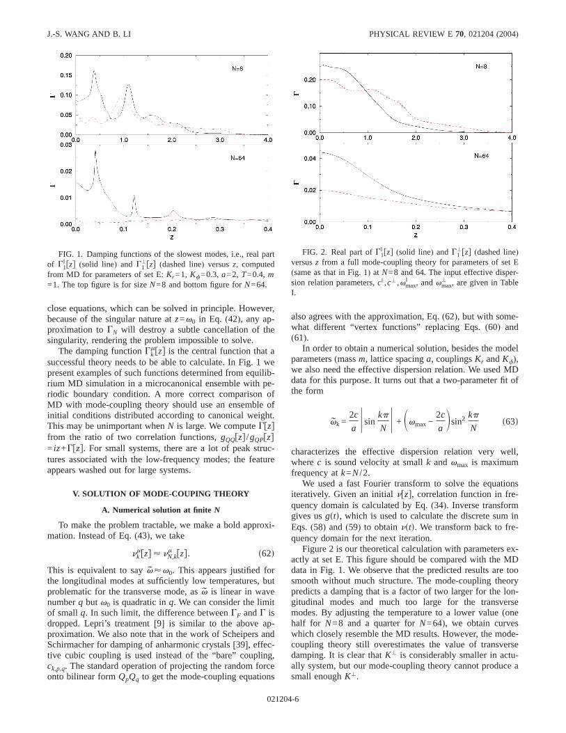
successful theory needs to be able to calculate. In Fig. 1 wepresent examples of such functions determined from equilib-rium MD simulation in a microcanonical ensemble with pe-riodic boundary condition. A more correct comparison ofMD with mode-coupling theory should use an ensemble ofinitial conditions distributed according to canonical weight.This may be unimportant whenN is large. We computeGfzgfrom the ratio of two correlation functions,gQQfzg /gQPfzg= iz+Gfzg. For small systems, there are a lot of peak struc-tures associated with the low-frequency modes; the featureappears washed out for large systems.

V. SOLUTION OF MODE-COUPING THEORY

A. Numerical solution at finite N

To make the problem tractable, we make a bold approxi-mation. Instead of Eq.(43), we take

nkmfzg < nN,k

m fzg. s62d

This is equivalent to sayv<v0. This appears justified forthe longitudinal modes at sufficiently low temperatures, butproblematic for the transverse mode, asv is linear in wavenumberq but v0 is quadratic inq. We can consider the limitof smallq. In such limit, the difference betweenGF andG isdropped. Lepri’s treatment[9] is similar to the above ap-proximation. We also note that in the work of Scheipers andSchirmacher for damping of anharmonic crystals[39], effec-tive cubic coupling is used instead of the “bare” coupling,ck,p,q. The standard operation of projecting the random forceonto bilinear formQpQq to get the mode-coupling equations

also agrees with the approximation, Eq.(62), but with some-what different “vertex functions” replacing Eqs.(60) and(61).

In order to obtain a numerical solution, besides the modelparameters(massm, lattice spacinga, couplingsKr andKf),we also need the effective dispersion relation. We used MDdata for this purpose. It turns out that a two-parameter fit ofthe form

vk =2c

aUsin

kp

NU + Svmax−

2c

aDsin2 kp

Ns63d

characterizes the effective dispersion relation very well,wherec is sound velocity at smallk and vmax is maximumfrequency atk=N/2.

We used a fast Fourier transform to solve the equationsiteratively. Given an initialnfzg, correlation function in fre-quency domain is calculated by Eq.(34). Inverse transformgives usgstd, which is used to calculate the discrete sum inEqs.(58) and (59) to obtainnstd. We transform back to fre-quency domain for the next iteration.

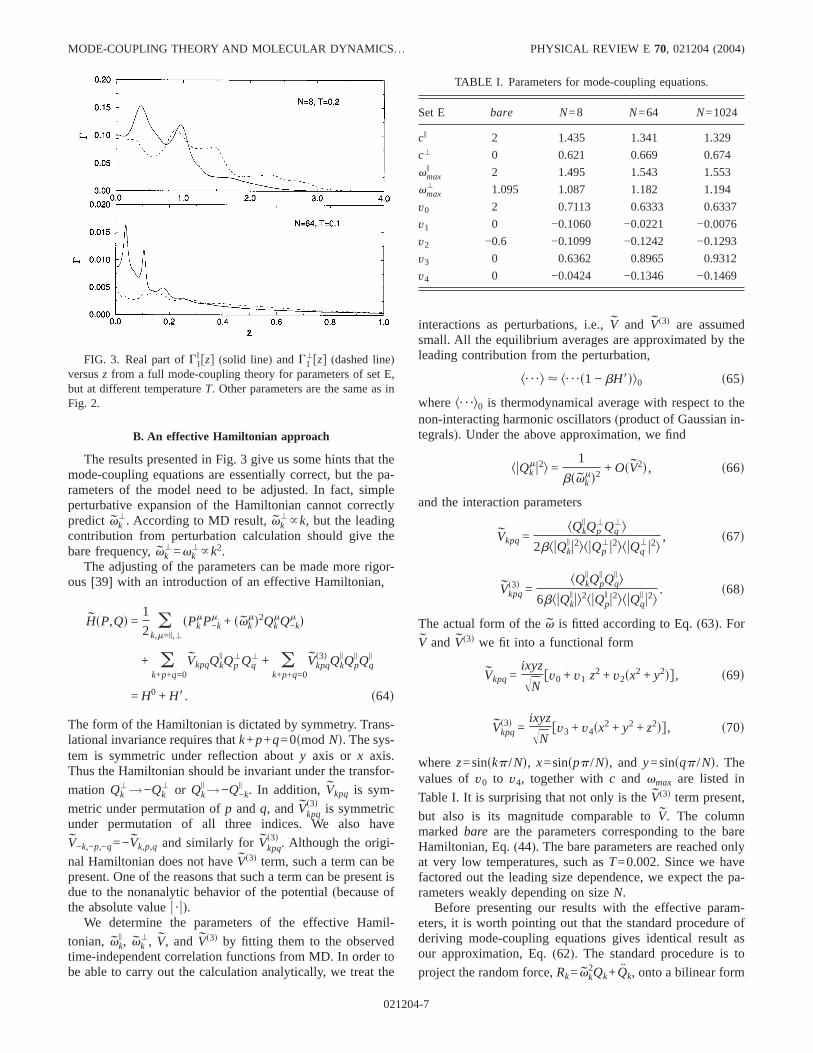
Figure 2 is our theoretical calculation with parameters ex-actly at set E. This figure should be compared with the MDdata in Fig. 1. We observe that the predicted results are toosmooth without much structure. The mode-coupling theorypredicts a damping that is a factor of two larger for the lon-gitudinal modes and much too large for the transversemodes. By adjusting the temperature to a lower value(onehalf for N=8 and a quarter forN=64), we obtain curveswhich closely resemble the MD results. However, the mode-coupling theory still overestimates the value of transversedamping. It is clear thatK' is considerably smaller in actu-ally system, but our mode-coupling theory cannot produce asmall enoughK'.

FIG. 1. Damping functions of the slowest modes, i.e., real partof G1

i fzg (solid line) and G1'fzg (dashed line) versusz, computed

from MD for parameters of set E:Kr =1, Kf=0.3, a=2, T=0.4, m=1. The top figure is for sizeN=8 and bottom figure forN=64.

FIG. 2. Real part ofG1i fzg (solid line) and G1

'fzg (dashed line)versusz from a full mode-coupling theory for parameters of set E(same as that in Fig. 1) at N=8 and 64. The input effective disper-sion relation parameters,ci ,c' ,vmax

i , andvmax' , are given in Table

I.


021204-6

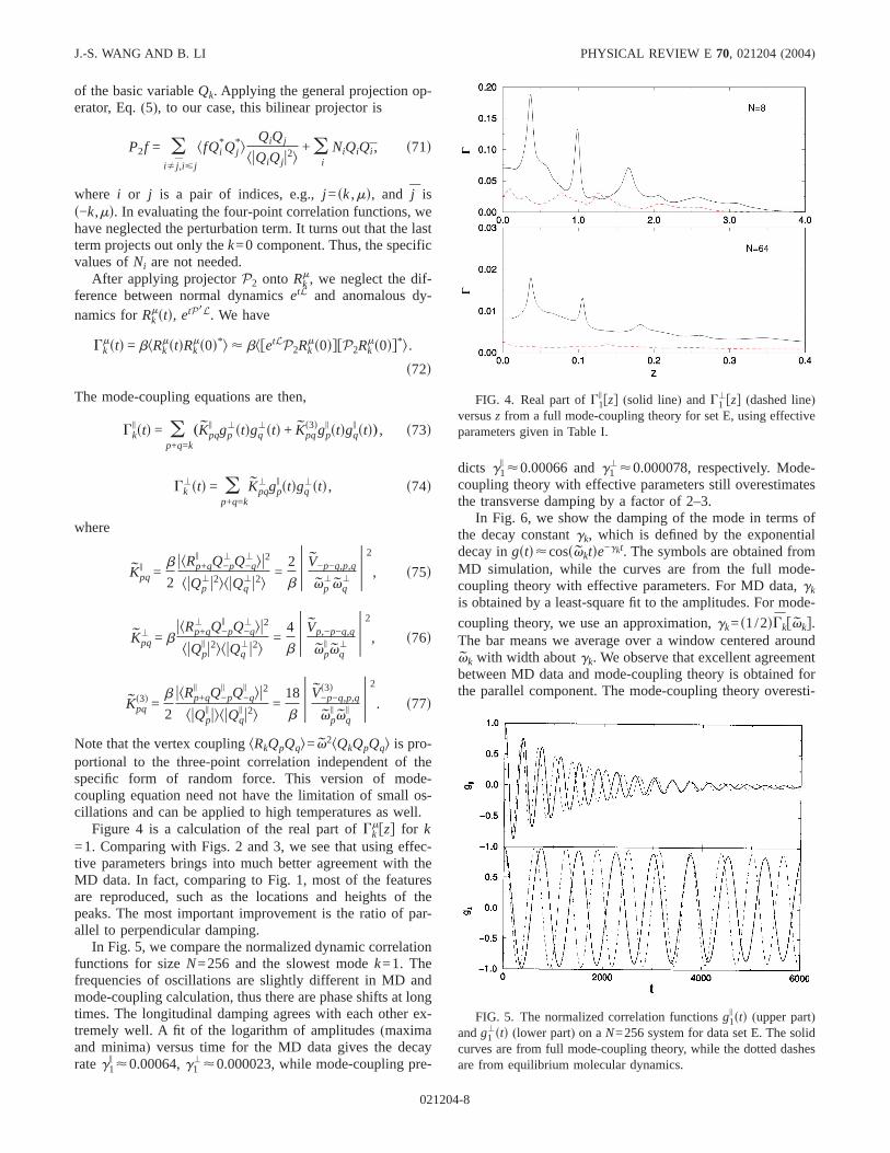
B. An effective Hamiltonian approach

The results presented in Fig. 3 give us some hints that themode-coupling equations are essentially correct, but the pa-rameters of the model need to be adjusted. In fact, simpleperturbative expansion of the Hamiltonian cannot correctlypredict vk

'. According to MD result,vk'~k, but the leading

contribution from perturbation calculation should give thebare frequency,vk

'=vk'~k2.

The adjusting of the parameters can be made more rigor-ous [39] with an introduction of an effective Hamiltonian,

HsP,Qd =1

2 ok,m=i,'

sPkmP−k

m + svkmd2Qk

mQ−km d

+ ok+p+q=0

VkpqQkiQp

'Qq' + o

k+p+q=0Vkpq

s3d QkiQp

i Qqi

= H0 + H8. s64d

The form of the Hamiltonian is dictated by symmetry. Trans-lational invariance requires thatk+p+q=0smod Nd. The sys-tem is symmetric under reflection abouty axis or x axis.Thus the Hamiltonian should be invariant under the transfor-

mation Qk'→−Qk

' or Qki →−Q−k

i . In addition, Vkpq is sym-

metric under permutation ofp andq, andVkpqs3d is symmetric

under permutation of all three indices. We also have

V−k,−p,−q=−Vk,p,q and similarly forVkpqs3d . Although the origi-

nal Hamiltonian does not haveVs3d term, such a term can bepresent. One of the reasons that such a term can be present isdue to the nonanalytic behavior of the potential(because ofthe absolute valueu ·u).

We determine the parameters of the effective Hamil-

tonian, vki , vk

', V, and Vs3d by fitting them to the observedtime-independent correlation functions from MD. In order tobe able to carry out the calculation analytically, we treat the

interactions as perturbations, i.e.,V and Vs3d are assumedsmall. All the equilibrium averages are approximated by theleading contribution from the perturbation,

k¯l < k¯s1 − bH8dl0 s65d

wherek¯l0 is thermodynamical average with respect to thenon-interacting harmonic oscillators(product of Gaussian in-tegrals). Under the above approximation, we find

kuQkmu2l =

1

bsvkmd2 + OsV2d, s66d

and the interaction parameters

Vkpq=kQk

iQp'Qq

'l2bkuQk

i u2lkuQp'u2lkuQq

'u2l, s67d

Vkpqs3d =

kQkiQp

i Qqi l

6bkuQki ul2kuQp

i u2lkuQqi u2l

. s68d

The actual form of thev is fitted according to Eq.(63). For

V and Vs3d we fit into a functional form

Vkpq=ixyzÎN

fv0 + v1 z2 + v2sx2 + y2dg, s69d

Vkpqs3d =

ixyzÎN

fv3 + v4sx2 + y2 + z2dg, s70d

wherez=sinskp /Nd, x=sinspp /Nd, and y=sinsqp /Nd. Thevalues ofv0 to v4, together withc and vmax are listed in

Table I. It is surprising that not only is theVs3d term present,

but also is its magnitude comparable toV. The columnmarkedbare are the parameters corresponding to the bareHamiltonian, Eq.(44). The bare parameters are reached onlyat very low temperatures, such asT=0.002. Since we havefactored out the leading size dependence, we expect the pa-rameters weakly depending on sizeN.

Before presenting our results with the effective param-eters, it is worth pointing out that the standard procedure ofderiving mode-coupling equations gives identical result asour approximation, Eq.(62). The standard procedure is to

project the random force,Rk=vk2Qk+Qk, onto a bilinear form


'fzg (dashed line)versusz from a full mode-coupling theory for parameters of set E,but at different temperatureT. Other parameters are the same as inFig. 2.

TABLE I. Parameters for mode-coupling equations.

Set E bare N=8 N=64 N=1024

ci 2 1.435 1.341 1.329

c' 0 0.621 0.669 0.674

vmaxi 2 1.495 1.543 1.553

vmax' 1.095 1.087 1.182 1.194

v0 2 0.7113 0.6333 0.6337

v1 0 −0.1060 −0.0221 −0.0076

v2 −0.6 −0.1099 −0.1242 −0.1293

v3 0 0.6362 0.8965 0.9312

v4 0 −0.0424 −0.1346 −0.1469


021204-7

of the basic variableQk. Applying the general projection op-erator, Eq.(5), to our case, this bilinear projector is

P2f = oiÞ j ,iø j

kfQi*Qj

*lQiQj

kuQiQju2l+ o

i

NiQiQi , s71d

where i or j is a pair of indices, e.g.,j =sk,md, and j iss−k,md. In evaluating the four-point correlation functions, wehave neglected the perturbation term. It turns out that the lastterm projects out only thek=0 component. Thus, the specificvalues ofNi are not needed.

After applying projectorP2 onto Rkm, we neglect the dif-

ference between normal dynamicsetL and anomalous dy-namics forRk

mstd, etP8L. We have

Gkmstd = bkRk

mstdRkms0d*l < bkfetLP2Rk

ms0dgfP2Rkms0dg*l.

s72d

The mode-coupling equations are then,

Gki std = o

p+q=k

„Kpqi gp

'stdgq'std + Kpq

s3dgpi stdgq

i std…, s73d

Gk'std = o

p+q=k

Kpq' gp

i stdgq'std, s74d

where

Kpqi =

b

2

ukRp+qi Q−p

' Q−q' lu2

kuQp'u2lkuQq

'u2l=

2

bU V−p−q,p,q

vp'vq

' U2

, s75d

Kpq' = b

ukRp+q' Q−p

i Q−q' lu2

kuQpi u2lkuQq

'u2l=

4

bU Vp,−p−q,q

vpivq

' U2

, s76d

Kpqs3d =

b

2

ukRp+qi Q−p

i Q−qi lu2

kuQpi ulkuQq

i u2l=

18

bU V−p−q,p,q

s3d

vpivq

i U2

. s77d

Note that the vertex couplingkRkQpQql=v2kQkQpQql is pro-portional to the three-point correlation independent of thespecific form of random force. This version of mode-coupling equation need not have the limitation of small os-cillations and can be applied to high temperatures as well.

Figure 4 is a calculation of the real part ofGkmfzg for k

=1. Comparing with Figs. 2 and 3, we see that using effec-tive parameters brings into much better agreement with theMD data. In fact, comparing to Fig. 1, most of the featuresare reproduced, such as the locations and heights of thepeaks. The most important improvement is the ratio of par-allel to perpendicular damping.

In Fig. 5, we compare the normalized dynamic correlationfunctions for sizeN=256 and the slowest modek=1. Thefrequencies of oscillations are slightly different in MD andmode-coupling calculation, thus there are phase shifts at longtimes. The longitudinal damping agrees with each other ex-tremely well. A fit of the logarithm of amplitudes(maximaand minima) versus time for the MD data gives the decayrateg1

i <0.00064,g1'<0.000023, while mode-coupling pre-

dicts g1i <0.00066 andg1

'<0.000078, respectively. Mode-coupling theory with effective parameters still overestimatesthe transverse damping by a factor of 2–3.

In Fig. 6, we show the damping of the mode in terms ofthe decay constantgk, which is defined by the exponentialdecay ingstd<cossvktde−gkt. The symbols are obtained fromMD simulation, while the curves are from the full mode-coupling theory with effective parameters. For MD data,gkis obtained by a least-square fit to the amplitudes. For mode-

coupling theory, we use an approximation,gk=s1/2dGkfvkg.The bar means we average over a window centered aroundvk with width aboutgk. We observe that excellent agreementbetween MD data and mode-coupling theory is obtained forthe parallel component. The mode-coupling theory overesti-


'fzg (dashed line)versusz from a full mode-coupling theory for set E, using effectiveparameters given in Table I.

FIG. 5. The normalized correlation functionsg1i std (upper part)

andg1'std (lower part) on aN=256 system for data set E. The solid

curves are from full mode-coupling theory, while the dotted dashesare from equilibrium molecular dynamics.


021204-8

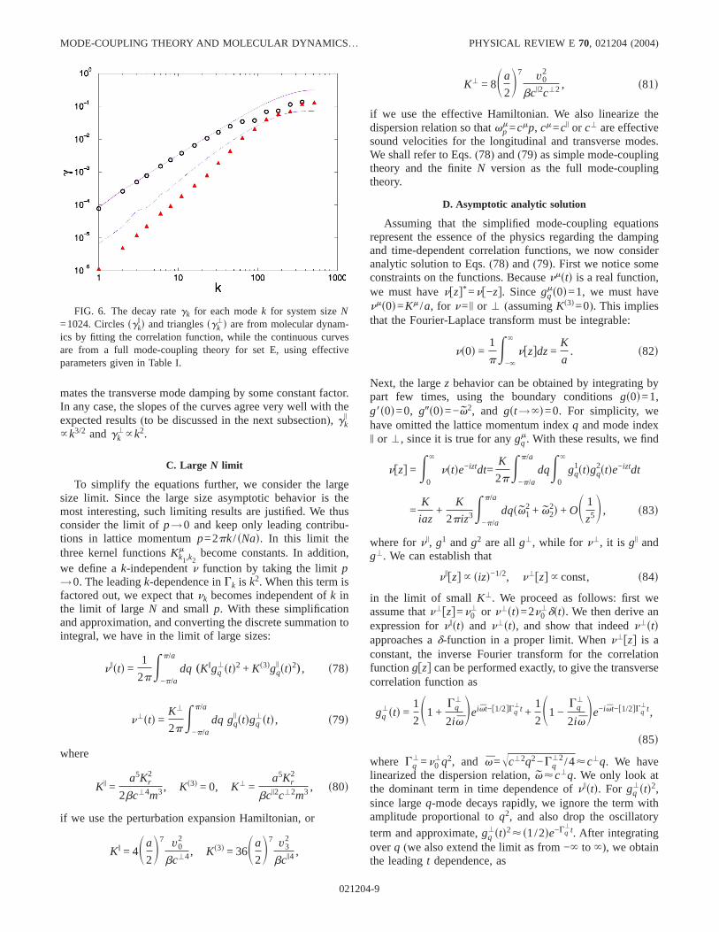
mates the transverse mode damping by some constant factor.In any case, the slopes of the curves agree very well with theexpected results(to be discussed in the next subsection), gk

i

~k3/2 andgk'~k2.

C. Large N limit

To simplify the equations further, we consider the largesize limit. Since the large size asymptotic behavior is themost interesting, such limiting results are justified. We thusconsider the limit ofp→0 and keep only leading contribu-tions in lattice momentump=2pk/ sNad. In this limit thethree kernel functionsKk1,k2

m become constants. In addition,we define ak-independentn function by taking the limitp→0. The leadingk-dependence inGk is k2. When this term isfactored out, we expect thatnk becomes independent ofk inthe limit of largeN and smallp. With these simplificationand approximation, and converting the discrete summation tointegral, we have in the limit of large sizes:

nistd =1

2pE

−p/a

p/a

dq „Kigq'std2 + Ks3dgq

i std2…, s78d

n'std =K'

2pE

−p/a

p/a

dq gqi stdgq

'std, s79d

where

Ki =a5Kr

2

2bc'4m3, Ks3d = 0, K' =a5Kr

2

bci2c'2m3 , s80d

if we use the perturbation expansion Hamiltonian, or

Ki = 4Sa

2D7 v0

2

bc'4, Ks3d = 36Sa

2D7 v3

2

bci4 ,

K' = 8Sa

2D7 v0

2

bci2c'2 , s81d

if we use the effective Hamiltonian. We also linearize thedispersion relation so thatvp

m=cmp, cm=ci or c' are effectivesound velocities for the longitudinal and transverse modes.We shall refer to Eqs.(78) and(79) as simple mode-couplingtheory and the finiteN version as the full mode-couplingtheory.

D. Asymptotic analytic solution

Assuming that the simplified mode-coupling equationsrepresent the essence of the physics regarding the dampingand time-dependent correlation functions, we now consideranalytic solution to Eqs.(78) and(79). First we notice someconstraints on the functions. Becausenmstd is a real function,we must havenfzg* =nf−zg. Sincegq

ms0d=1, we must havenms0d=Km /a, for n=i or ' (assumingKs3d=0). This impliesthat the Fourier-Laplace transform must be integrable:

ns0d =1

pE

−`

`

nfzgdz=K

a. s82d

Next, the largez behavior can be obtained by integrating bypart few times, using the boundary conditionsgs0d=1,g8s0d=0, g9s0d=−v2, and gst→`d=0. For simplicity, wehave omitted the lattice momentum indexq and mode indexi or ', since it is true for anygq

m. With these results, we find

nfzg =E0

`

nstde−iztdt=K

2pE

−p/a

p/a

dqE0

`

gq1stdgq

2stde−iztdt

=K

iaz+

K

2piz3E−p/a

p/a

dqsv12 + v2

2d + OS 1

z5D , s83d

where forni, g1 andg2 are allg', while for n', it is gi andg'. We can establish that

nifzg ~ sizd−1/2, n'fzg ~ const, s84d

in the limit of small K'. We proceed as follows: first weassume thatn'fzg=n0

' or n'std=2n0'dstd. We then derive an

expression fornistd and n'std, and show that indeedn'stdapproaches ad-function in a proper limit. Whenn'fzg is aconstant, the inverse Fourier transform for the correlationfunctiongfzg can be performed exactly, to give the transversecorrelation function as

gq'std =

1

2S1 +

Gq'

2ivDeivt−f1/2gGq

't +1

2S1 −

Gq'

2ivDe−ivt−f1/2gGq

't,

s85d

where Gq'=n0

'q2, and v=Îc'2q2−Gq'2/4<c'q. We have

linearized the dispersion relation,v<c'q. We only look atthe dominant term in time dependence ofnistd. For gq

'std2,since largeq-mode decays rapidly, we ignore the term withamplitude proportional toq2, and also drop the oscillatory

term and approximate,gq'std2<s1/2de−Gq

't. After integratingoverq (we also extend the limit as from −to `), we obtainthe leadingt dependence, as

FIG. 6. The decay rategk for each modek for system sizeN=1024. Circlessgk

i d and trianglessgk'd are from molecular dynam-

ics by fitting the correlation function, while the continuous curvesare from a full mode-coupling theory for set E, using effectiveparameters given in Table I.


021204-9

nistd <Ki

4Î 1

pn0't

. s86d

If the oscillatory terms are kept, they only contribute an ex-

ponentially small term,e−sc'd2t/n0'

; and theq2 terms give acontribution that decays much faster, ast−3/2. The contribu-tion from Ks3d term can be neglected, because it decays ast−2/3 [due to Eq.(91)]. But this term does provide a crossoverfrom z−1/3 for intermediatez to the asymptoticz−1/2 for verysmall z. The Fourier-Laplace transform gives

nifzg <Ki

4Î 1

in0'z

= bsizd−1/2. s87d

We now get an expression for the longitudinal correlationfunction. Formally, it is given by the inverse transform

gqi std =

1

2pE

−`

` − iz − Gqi fzg

z2 − ciq2 − izGqi fzg

eiztdz, s88d

where Gqi fzg=q2nifzg=bq2/Îiz, b= 1

4Ki /În0'. The dominant

contribution is fromz when the denominator is close to zero.The integral can be approximately estimated by the residuetheorem. By location the poles

z2 − ci2q2 − Îiz bq2 = 0, s89d

we obtain the dispersion relation forgqi std. In the limit of

small q, we find

z< ciq + ig0q3/2, s90d

whereg0=sÎ2/16dKi /Îcin0'. Therefore,

gqi std < e−g0q3/2tcossciqtd. s91d

Similarly with the dispersion relation for the transversemode,z<c'q+s1/2din0q

2, we can compute

n'std =K'

pE

0

`

dq e−g0q3/2t−f1/2gn0'q2t cossciqtdcossc'qtd

<K'Î 1

8pn0't

se−sci − c'd2/2n0't + e−sci + c'd2/2n0

'td .

s92d

We have neglected theg0 term. Sinceuci−c'u is smaller thanci+c', we drop the second term. We symmetrically extendthe function. Note thatn'std can be casted into the functionalform

fsstd =1

2Îs

p

e−sut

Îutu, s =

sci − c'd2

2n0' , s93d

which has the property that

E−`

`

fsstddt = 1, for all s . 0. s94d

Thus fsstd behaves as ad-function ass→`:

n'std <K'

uci − c'udstd. s95d

This allows us to identify the constantn0'= 1

2K' / uci−c'u.The condition fors→` is the same asn0

'→0 or K'→0.Since K' /Ki=2sc' /cid2 [cf., Eq. (80)], small K' also im-plies smallc'.

Although the above derivation suggests that the result isvalid only for the special limit. But in fact, this is also theasymptotic result in the limitz→0. To show this, we notethat the asymptotic behavior is picked up by the scalingliml→0ldnflzg<nfzg. If this is true, thennfzg~z−d. Thisscaling limit coincides with the limit ofK'→0.

E. Numerical solution of the simple theory

For the simple mode-coupling theory that we have alreadytaken the largeN limit, we can also apply the fast Fouriertransform method. However, we find that a direct numericalintegration in frequency space is much more accurate. Forexample,n'fzg is expressed as

n'fzg =K'

s2pd3E−`

+`

dvE−`

+`

dv8 2 F'sv,v8dSP1

isz− v − v8d

+ pdsz− v − v8dD , s96d

where P stands for Cauchy principal value and

F'sv,v8d =E0

p/a

gisq,vdg'sq,v8ddq, s97d

gi,'sq,vd =− iv − ni,'fvgq2

v2 − sci,'d2q2 − ivni,'fvgq2 . s98d

When the linear approximation is made to the dispersionrelations, the integral overq can be performed analytically.We only need to do a 2D integral overv andv8. The prin-cipal value integral is taken care by locating exactly the sin-gularity. Since the integration routine needs a smooth func-tion nfzg, we fit the results by a Padé approximation[invariableiz or sizd1/3]. The procedure is iterated several timesfor convergence. This is programmed inMATHEMATICA . Itturns out that it is essential to have more than double preci-sion accuracy in the integration routine in order for the sin-gular integrals to properly converge. Some results of thiscalculation are already presented in Ref.[31].

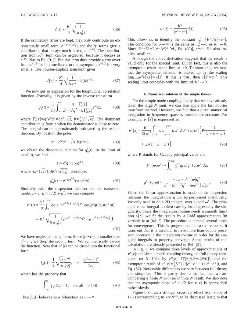
In Fig. 7, we compare three levels of approximations ofnmfzg: the simple mode-coupling theory, the full theory com-puted on N=1024 by nmfzg=G1

mfzg / f2p / sNadg2, and theasymptotic result ofn'fzg= 1

2K's1/uci−c'u+1/uci+c'ud, andEq. (87). Noticeable differences are seen between full theoryand simplified. This is partly due to the fact that we arecomparing a finiteN with an infiniteN result. We also notethat the asymptotic slope of −1/2 fornifzg is approachedrather slowly.

Figure 8 shows a stronger crossover effect from slope of1/3 (corresponding tok~N2/5, to be discussed later) to that


021204-10

of the true asymptotic law of 1/2. This set of curves corre-sponds to data set J.

F. Scaling solution of the simple theory

We now look at some of the scaling properties that areimplied from Eqs. (78) and (79). First, we consider thesimple case ofK=Ki=K', Ks3d=0, and c=ci=c'. In thiscase the two equations degenerate into one equation given byLepri [9]. By measuring frequency in terms ofc (i.e., con-sider variablez/c) we can scale awayc, thus the followingequation is an exact scaling

nsz;K,c,ad = cnsz/c;K/c2,1,ad, s99d

wheren is a function ofz with parametersK, c, anda that wehave written out explicitly. This equation tells us that out of

the three parameters that characterize the solution, we canpick two as independent. The “shapes” of the solutions areall the same forK /c2=const. Without loss of generality, wecan fixK=1. Next, we consider a general scaling solution ofthe form

nslz;K,lDcc,lDaad < l−dnsz;K,c,ad. s100d

Substituting this scaling form into Eq.(96), by requiring thatthe result must be consistent, we obtain the following condi-tions:

2Dq − d − 1 = 0, s101d

Dc + Dq − 1 = 0, s102d

1 − Dq = d, s103d

Da + Dq = 0, s104d

where Dq is scaling exponent associated with integrationvariableq, q→lDqq. A unique solution to the set of linearequations is obtained,d=1/3, Dc=1/3, Da=−2/3, andDq=2/3.Since Eq.(100) is (approximately) valid for anyl, wecan choosel=1/z. This scaling solution implies that

nsz;K,c,ad < z−1/3ns1;K,c/z1/3,z2/3ad. s105d

Power-law behaviorz−1/3 is obtained in the limit of smallz,relatively largec, and smalla, if ns1,K ,` ,0d is finite. Thecrossover to other behavior occurs at largez,c3 and z,a−3/2.

A simple dimension analysis also leads to thez−1/3 factor.Let the dimension of length and time beL and T, respec-tively. Then the dimensions of relevant quantities arefzg=T−1, fcg=LT−1, fag=L, fng=L2T−1, and fKg=L3T−2. Fromthe five quantities, we can construct three dimensionlessvariables

P1 =n

z−1/3K2/3, P2 =c

z a, P3 =

K

ac2 . s106d

If there is any relation between thePi’s, it must be in theform P1= fsP2,P3d (Buckingham Pi theorem[40]), or

nfzg = z−1/3K2/3fSza

c,

K

ac2D , s107d

where f is an arbitrary, dimensionless function. This result,of course, is consistent with Eq.(100). This also suggeststhat the scaling is not approximate, but an exact result.

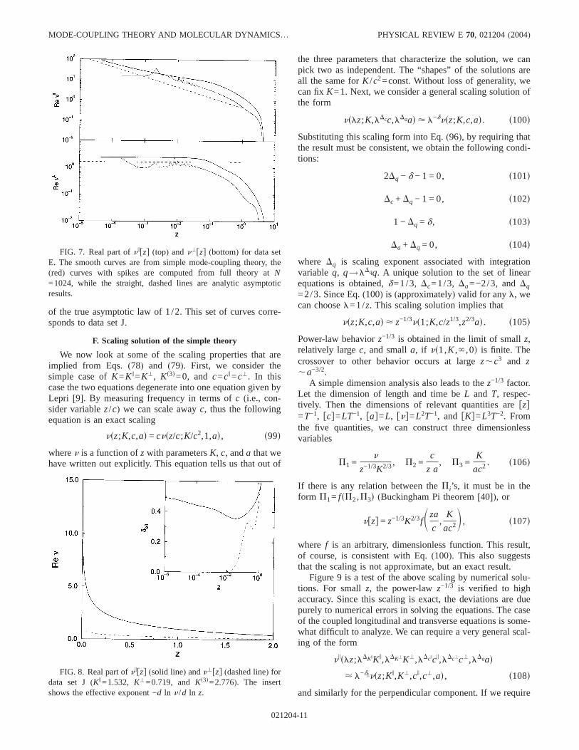
Figure 9 is a test of the above scaling by numerical solu-tions. For smallz, the power-lawz−1/3 is verified to highaccuracy. Since this scaling is exact, the deviations are duepurely to numerical errors in solving the equations. The caseof the coupled longitudinal and transverse equations is some-what difficult to analyze. We can require a very general scal-ing of the form

nislz;lDKiKi,lDK'K',lDcici,lDc'c',lDaad

< l−dinsz;Ki,K',ci,c',ad, s108d

and similarly for the perpendicular component. If we require

FIG. 7. Real part ofnifzg (top) andn'fzg (bottom) for data setE. The smooth curves are from simple mode-coupling theory, the(red) curves with spikes are computed from full theory atN=1024, while the straight, dashed lines are analytic asymptoticresults.

FIG. 8. Real part ofnifzg (solid line) andn'fzg (dashed line) fordata set J(Ki=1.532, K'=0.719, andKs3d=2.776). The insertshows the effective exponent −d ln n /d ln z.


021204-11

for consistency of scaling for both longitudinal and trans-verse components, we find that the only scaling solution isthe symmetric solution, i.e., the scaling discussed above withidentical longitudinal and transverse scaling exponents. If weabandon the exact scaling for the transverse component andlook only at longitudinal component, we can require that

d' = 2Dq − 1, s109d

di = 1 −DKi − Dq, s110d

Dc' = 1 −Dq. s111d

As before we can require that there is no scaling for thecoupling constantKi without loss of generality(i.e., DKi =0),the above equations imply a relation

2di + d' = 1. s112d

In particular, ifd'=0, we must havedi=1/2 andDc'=1/2.This is consistent with the fact that the scaling region ofdi

=1/2 is obtained for smallc'.A complete and clear scaling picture is still lacking. From

the numerical solution, we observe that besides well-characterized scaling regimes, there are also plenty of inter-mediate regions and crossovers. For very largec' and smallK', or smallc' and largeK', the behavior of the solutionsare difficult to characterize.

VI. GREEN-KUBO FORMULA

In this section, we make the connection of the damping ofmodes with thermal conduction. The starting point is theGreen-Kubo formula for transport coefficient:

k =1

kBT2aNE

0

`

kJstdJs0dldt. s113d

For the special case of heat conduction in a 1D chain, it isbetter to callk heat conductance rather than heat conductiv-

ity. In analogous to electric circuit, the heat conductance re-lates the temperature gradient to energy current(Fourierlaw),

I = − kdT

dx. s114d

The quantityJstd is related to energy current byJ= IaN. Thecentral quantity that we compute in equilibrium and nonequi-librium heat conduction is the(total) heat currentJ. Since theheat current is a macroscopic concept determined by the con-servation of(internal) energy, a microscopic version of it isnot unique. The current expression must satisfy the energycontinuity equation in the long-wave limit. We derive an ex-pression starting fromJ=oi dsr ihid /dt, where the local en-ergy per particle is hi =

14KrfsuDr i−1u−ad2+suDr iu−ad2g

+Kf cosfi +pi2/ s2md. By regrouping some of the terms us-

ing translational invariance, we arrive at the heat current perparticle:

m j i = − Dr ifspi + pi+1d ·Gsidg− Dr i−1fspi + pi−1d ·Gsi − 1dg

+ Dr i−1fpi ·Hsi − 2,i − 1,i − 1dg

+ Dr ifpi ·Hsi + 1,i + 1,idg + pihi , s115d

where Gsid= 14KrsuDr iu−adni, Hsi , j ,kd=Kfsni +nk cosf jd /

uDr ku, ni is a unit vector in direction ofDr i =r i+1−r i. Thetotal heat current inx direction,J=oi j x,i is the quantity ap-pearing in the Green-Kubo formula. It is equal to the mac-roscopic heat current density(energy per unit area per unittime) integrated over a volume.

For theoretical analysis, we need to expressJ in terms ofthe dynamical variablesPk andQk. A general expression willbe rather complicated. Again as in mode-coupling approach,we consider small oscillation expansions and only the lead-ing contributions. Neglecting the nonlinear contribution ofOsQk

3d, we obtain

J = ok,m

bkmQk

mP−km , bk

m = ivkm ] vk

m

] S2pk

NaD , s116d

wherevkm is the bare dispersion relation given by Eqs.(45)

and(46). More general expression in a quantum-mechanicalframework including the cubic terms is given in Ref.[42].An approximation for the correlation function of the currentcan be obtained, again using a dynamic mean-field approxi-mation, as

kJstdJs0dl = ok,m

ubkmu2hkQk

mstdQ−km s0dlkPk

mstdP−km s0dl

+ kQkmstdP−k

m s0dl2j. s117d

The above expression can be further simplified by the ap-

proximationPkm=Qk

m< vkmQk

m. We find

FIG. 9. Real part (top) and imaginary part(bottom) ofl1/3nslz;K ,l1/3c,l−2/3ad versusz for K=c=a=1 andl=1 (solidline), 1/8 (open circles), and 8(crosses).


021204-12

kJstdJs0dl < ok,mU bk

m

bvkmU2

gkmstd2

<aNscid2

2pb2 E0

`

cos2svpi tde−2gp

itdp~

Nscid2

b2 t−1/s2−did.

s118d

We have dropped the contribution from the perpendicularcomponent because it decays much faster(due to an extrap2

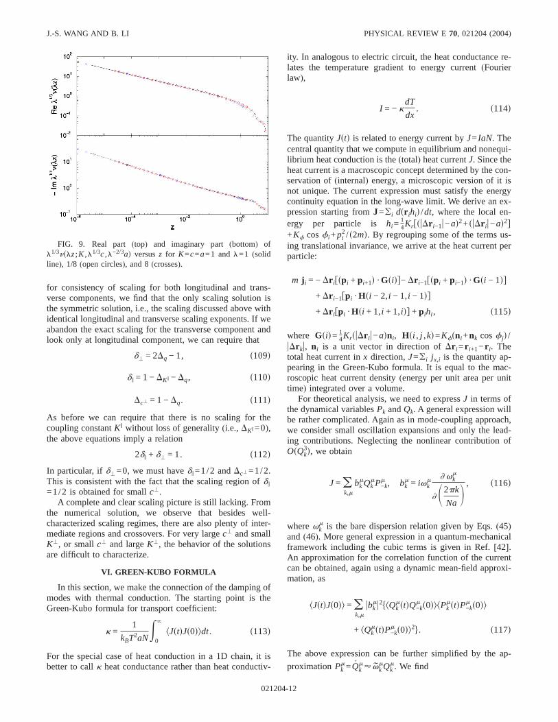
factor in the integrand). We compare the mode-coupling re-sult of Green-Kubo integrand with that of MD in Fig. 10. Wehave used Eq.(117) for the mode-coupling calculation. Notethat the correlation functionskQstdQs0d*l, kPstdPs0d*l, andkQstdPs0d*l are simply related in frequency domain throughEq. (32). The agreement is reasonable with the largest devia-tion about a factor of 2. The asymptotic behavior oft−2/3 isconsistent with both sets of results.

The heat conductance on a finite lattice is sensitive toboundary conditions. Clearly, in the mode-coupling formula-tion, we have used periodic boundary condition. If we inte-grate over time from 0 to first on the second line of Eq.(118), we obtaink~edp/gp. On a finite lattice we have alower momentum cutoff, 2p / sNad. The size dependence ofthe conductance on finite lattice is then

kN ~ N1−di. s119d

Sincedi=1/2, k~ÎN. This result is in agreement with thatof Deutsch and Narayan for a model(the random collisionmodel) where transverse motion is taken into account onlystochastically[16].

In Fig. 11, the mode-coupling result ofkN is comparedwith equilibrium MD result with periodic boundary condi-tions. Excellent 1/2 power is observed for the mode-coupling result. We found it is rather difficult to get con-

verged value from MD. But the results are consistent with aÎN law.

The relation of the mode-coupling theory with the resultsof nonequilibrium situation of low- and high-temperatureheat-baths at the ends is not clear cut. The standard assump-tion is that the correlation should be cut off by a time scale oforderN due to the interaction with the heat baths. Finite sizeresult is obtained by integrating the power-law decay to atime of OsNd. This gives us the asymptotic behavior for theconductance at largeN as

kN ~ Na, a = 1 −1

2 − di

. s120d

Since we finddi=1/2 for small K', the thermal conductiondiverges asN1/3. WhenKs3d is sufficiently large, we observeN2/5.

VII. NONEQUILIBRIUM MD STUDY

A. MD simulation details

We note that the interaction potential is not smooth at thepoint when two particles overlap. This can cause numericalinstability. Thus, we replaced the original potential with amodified one,

Dr = ur i+1 − r iu → Dr8 = Dr +e2

Dr + e, s121d

which smooths out the discontinuous derivatives atDr =0with a small correction of ordere2. In addition to replacingthe spring potential by1

2KrsDr8−ad2, we also replace thecosine term by

FIG. 10. The Green-Kubo integrand from MD(circles) andmode-coupling theory(curve) for set E with sizeN=1024. Thestraight has a slope −2/3. The insert shows the same data on alinear scale.

FIG. 11. The finite lattice conductance defined by Green-Kuboformula at parameter set E. Solid circles are from full mode-coupling theory; the triangles are from molecular dynamics withperiodic boundary condition; the straight lines have slope of 1/2.


021204-13

cosfi8 = −Dr i−1 · Dr i

Dr i−18 Dr i8, s122d

so that the value is well defined for all positionsr i. In actualsimulation, we have used very smalle,10−3 to 10−4 so thatits effect should be comparable to error caused by finite time-steph. We also used largee as a way of simulating a slightlydifferent model to study the robustness of the results. Wesolve the system of equations[41]

dpi

dt= 5 f i − jLpi , if i , Nw;

f i , if N − Nw . i ù Nw;

f i − jHpi , if i ù N − Nw;

s123d

wheref i is the total force acting on thei-th particle,jL andjHobey the equation

djL,H

dt=

1

Q2S− 1 +1

kBTL,HNwo

i

pi2

mD , s124d

whereTL andTH are the temperatures of the two heat bathsat the ends. The summation is over the particles belonging tothe heat bath. We have used four particles for the Nosé-Hoover heat baths, with extra first two and last two particlesat fixed positions. The coupling parameterQ is taken to be 1.For the central part, we used a second-order symplectic al-gorithm (or equivalently, the velocity Verlet algorithm),while for the heat bath, we used a simple difference schemeaccurate to second order inh for j.

Although the total energy(Hamiltonian) is no longer aconserved quantity when the heat bath is introduced, theabove equation still has a conserved quantity of similar char-acter:

Hsp,qd + ox=L,H

NwkBTxS1

2Q2jx

2 +E0

t

jxdtD . s125d

This quantity can be used to monitor the stability of thealgorithm. Since we run for very long time steps of108–1010, it is essential that the algorithm is stable over anextended period of time. Even with a symplectic algorithm,stability is not guaranteed by merely taking smallhs,10−4d.Thus, we adjusted the conserved quantity, Eq.(125), to itsstarting value after certain number of steps.

B. Heat conductance results

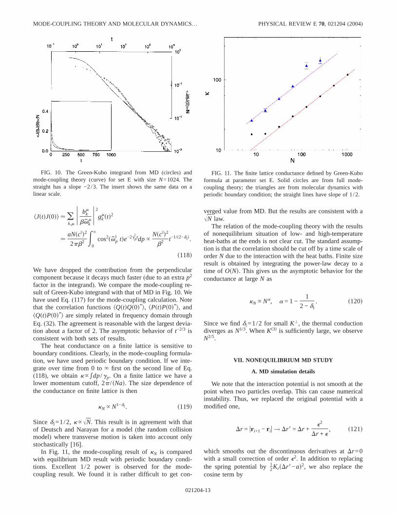
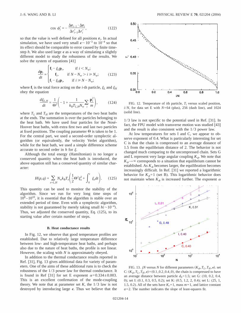
In Fig. 12, we observe that good temperature profiles areestablished. Due to relatively large temperature differencebetween low- and high-temperature heat baths, and perhapsalso due to the nature of heat baths, the profile is not linear.However, the scaling withN is approximately obeyed.

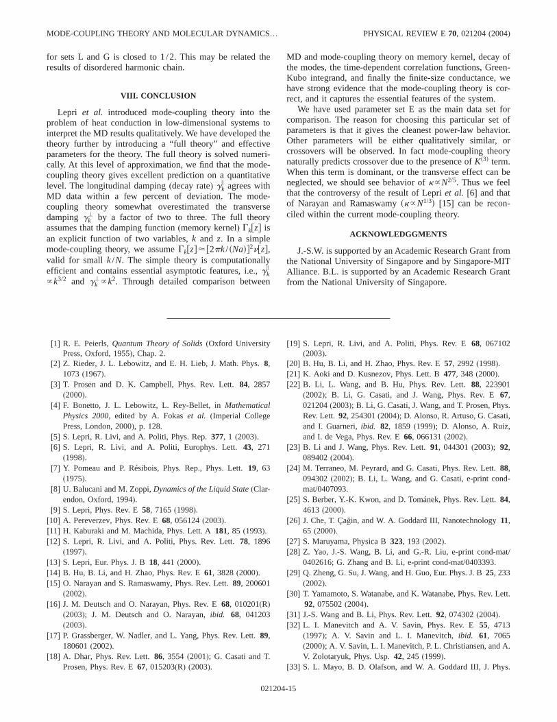
In addition to the thermal conductance results reported inRef. [31], Fig. 13 gives additional data for variety of param-eters. One of the aims of these additional runs is to check therobustness of the 1/3 power law for thermal conductance. Itis found in Ref [31] for set E exponenta=0.334±0.003.This is an excellent confirmation of the mode-couplingtheory. We note that at parameter setK, the 1/3 law is notdestroyed by introducing largee. Thus we believe that the

1/3 law is not specific to the potential used in Ref.[31]. Infact, the FPU model with transverse motion was studied[43]and the result is also consistent with the 1/3 power law.

At low temperatures for sets I and C, we appear to ob-serve exponent of 0.4. What is particularly interesting for setC is that the chain is compressed to an average distance of1.5 from the equilibrium distance of 2. The behavior is notchanged much comparing to the uncompressed chain. Sets Gand L represent very large angular couplingKf. We note thatKf→` corresponds to a situation that equilibrium cannot beestablished. AsKf becomes larger, the equilibration becomesincreasingly difficult. In Ref.[31] we reported a logarithmicbehavior forKf=1 (set B). This logarithmic behavior doesnot maintain whenKf is increased further. The exponenta

FIG. 12. Temperature ofith particle,Ti versus scaled position,i /N, for data set E withN=64 (plus), 256 (dash line), and 1024(solid line).

FIG. 13. jN versusN for different parameterssKf ,TL ,TH ,ed. setC: sKf ,TL ,TH ,ed=s0.1,0.2,0.4,0d, the chain is compressed to havean average distance between particled0=1.5; set G:(10, 0.2, 0.4,0); set I: (0.1, 0.3, 0.5, 0.2); set K: (0.5, 1.2, 2, 0.4); set L: (25, 1,1.5, 0.2). All of the sets haveKr =1, massm=1, and lattice constanta=2. The number indicates the slope of least-squares fit.


021204-14

for sets L and G is closed to 1/2. This may be related theresults of disordered harmonic chain.

VIII. CONCLUSION

Lepri et al. introduced mode-coupling theory into theproblem of heat conduction in low-dimensional systems tointerpret the MD results qualitatively. We have developed thetheory further by introducing a “full theory” and effectiveparameters for the theory. The full theory is solved numeri-cally. At this level of approximation, we find that the mode-coupling theory gives excellent prediction on a quantitativelevel. The longitudinal damping(decay rate) gk

i agrees withMD data within a few percent of deviation. The mode-coupling theory somewhat overestimated the transversedamping gk

' by a factor of two to three. The full theoryassumes that the damping function(memory kernel) Gkfzg isan explicit function of two variables,k and z. In a simplemode-coupling theory, we assumeGkfzg<f2pk/ sNadg2nfzg,valid for small k/N. The simple theory is computationallyefficient and contains essential asymptotic features, i.e.,gk

i

~k3/2 and gk'~k2. Through detailed comparison between

MD and mode-coupling theory on memory kernel, decay ofthe modes, the time-dependent correlation functions, Green-Kubo integrand, and finally the finite-size conductance, wehave strong evidence that the mode-coupling theory is cor-rect, and it captures the essential features of the system.

We have used parameter set E as the main data set forcomparison. The reason for choosing this particular set ofparameters is that it gives the cleanest power-law behavior.Other parameters will be either qualitatively similar, orcrossovers will be observed. In fact mode-coupling theorynaturally predicts crossover due to the presence ofKs3d term.When this term is dominant, or the transverse effect can beneglected, we should see behavior ofk~N2/5. Thus we feelthat the controversy of the result of Lepriet al. [6] and thatof Narayan and Ramaswamysk~N1/3d [15] can be recon-ciled within the current mode-coupling theory.

ACKNOWLEDGGMENTS

J.-S.W. is supported by an Academic Research Grant fromthe National University of Singapore and by Singapore-MITAlliance. B.L. is supported by an Academic Research Grantfrom the National University of Singapore.

[1] R. E. Peierls,Quantum Theory of Solids(Oxford UniversityPress, Oxford, 1955), Chap. 2.

[2] Z. Rieder, J. L. Lebowitz, and E. H. Lieb, J. Math. Phys.8,1073 (1967).

[3] T. Prosen and D. K. Campbell, Phys. Rev. Lett.84, 2857(2000).

[4] F. Bonetto, J. L. Lebowitz, L. Rey-Bellet, inMathematicalPhysics 2000, edited by A. Fokaset al. (Imperial CollegePress, London, 2000), p. 128.

[5] S. Lepri, R. Livi, and A. Politi, Phys. Rep.377, 1 (2003).[6] S. Lepri, R. Livi, and A. Politi, Europhys. Lett.43, 271

(1998).[7] Y. Pomeau and P. Résibois, Phys. Rep., Phys. Lett.19, 63

(1975).[8] U. Balucani and M. Zoppi,Dynamics of the Liquid State(Clar-

endon, Oxford, 1994).[9] S. Lepri, Phys. Rev. E58, 7165(1998).

[10] A. Pereverzev, Phys. Rev. E68, 056124(2003).[11] H. Kaburaki and M. Machida, Phys. Lett. A181, 85 (1993).[12] S. Lepri, R. Livi, and A. Politi, Phys. Rev. Lett.78, 1896

(1997).[13] S. Lepri, Eur. Phys. J. B18, 441 (2000).[14] B. Hu, B. Li, and H. Zhao, Phys. Rev. E61, 3828(2000).[15] O. Narayan and S. Ramaswamy, Phys. Rev. Lett.89, 200601

(2002).[16] J. M. Deutsch and O. Narayan, Phys. Rev. E68, 010201(R)

(2003); J. M. Deutsch and O. Narayan,ibid. 68, 041203(2003).

[17] P. Grassberger, W. Nadler, and L. Yang, Phys. Rev. Lett.89,180601(2002).

[18] A. Dhar, Phys. Rev. Lett.86, 3554 (2001); G. Casati and T.Prosen, Phys. Rev. E67, 015203(R) (2003).

[19] S. Lepri, R. Livi, and A. Politi, Phys. Rev. E68, 067102(2003).

[20] B. Hu, B. Li, and H. Zhao, Phys. Rev. E57, 2992(1998).[21] K. Aoki and D. Kusnezov, Phys. Lett. B477, 348 (2000).[22] B. Li, L. Wang, and B. Hu, Phys. Rev. Lett.88, 223901

(2002); B. Li, G. Casati, and J. Wang, Phys. Rev. E67,021204(2003); B. Li, G. Casati, J. Wang, and T. Prosen, Phys.Rev. Lett. 92, 254301(2004); D. Alonso, R. Artuso, G. Casati,and I. Guarneri,ibid. 82, 1859 (1999); D. Alonso, A. Ruiz,and I. de Vega, Phys. Rev. E66, 066131(2002).

[23] B. Li and J. Wang, Phys. Rev. Lett.91, 044301(2003); 92,089402(2004).

[24] M. Terraneo, M. Peyrard, and G. Casati, Phys. Rev. Lett.88,094302(2002); B. Li, L. Wang, and G. Casati, e-print cond-mat/0407093.

[25] S. Berber, Y.-K. Kwon, and D. Tománek, Phys. Rev. Lett.84,4613 (2000).

[26] J. Che, T. Çağin, and W. A. Goddard III, Nanotechnology11,65 (2000).

[27] S. Maruyama, Physica B323, 193 (2002).[28] Z. Yao, J.-S. Wang, B. Li, and G.-R. Liu, e-print cond-mat/

0402616; G. Zhang and B. Li, e-print cond-mat/0403393.[29] Q. Zheng, G. Su, J. Wang, and H. Guo, Eur. Phys. J. B25, 233

(2002).[30] T. Yamamoto, S. Watanabe, and K. Watanabe, Phys. Rev. Lett.

92, 075502(2004).[31] J.-S. Wang and B. Li, Phys. Rev. Lett.92, 074302(2004).[32] L. I. Manevitch and A. V. Savin, Phys. Rev. E55, 4713

(1997); A. V. Savin and L. I. Manevitch,ibid. 61, 7065(2000); A. V. Savin, L. I. Manevitch, P. L. Christiansen, and A.V. Zolotaryuk, Phys. Usp.42, 245 (1999).

[33] S. L. Mayo, B. D. Olafson, and W. A. Goddard III, J. Phys.


021204-15

Chem. 94, 8897(1990).[34] J. Tersoff, Phys. Rev. B37, 6991(1988).[35] R. Kubo, M. Toda, and N. Hashitsume,Statistical Physics II,

2nd ed.(Springer, Berlin, 1992), pp. 97–108.[36] R. Zwanzig, J. Chem. Phys.33, 1338(1960).[37] H. Mori, Prog. Theor. Phys.33, 424 (1965).[38] K. Huang,Statistical Mechanics, 2nd ed.(Wiley, New York,

1987).

[39] J. Scheipers and W. Schirmacher, Z. Phys. B: Condens. Matter103, 547 (1997).

[40] E. Buckingham, Phys. Rev.4, 345 (1914).[41] For general aspects on molecular dynamics, see, e.g., D. Fren-

kel and B. Smit,Understanding Molecular Simulation: FromAlgorithms to Applications(Academic, New York, 1996).

[42] R. J. Hardy, Phys. Rev.132, 168 (1963).[43] B. Li, J.-H. Lan, and L. Wang(unpublished).


021204-16

Documents

Mode-coupling theory and molecular dynamics simulation …polymer.chph.ras.ru/asavin/teplopr/wl04pre.pdf · Mode-coupling theory and molecular dynamics simulation for heat conduction