Model-Predictive Control of Discrete Hybrid Stochastic Automata

IEEE TRANSACTIONS ON AUTOMATIC CONTROL, VOL. 56, NO. 6, JUNE 2011 1307

Model-Predictive Control of Discrete HybridStochastic Automata

Alberto Bemporad, Fellow, IEEE, and Stefano Di Cairano, Member, IEEE

Abstract—This paper focuses on optimal and receding horizoncontrol of a class of hybrid dynamical systems, called DiscreteHybrid Stochastic Automata (DHSA), whose discrete-state tran-sitions depend on both deterministic and stochastic events. Afinite-time optimal control approach “optimistically” determinesthe trajectory that provides the best tradeoff between trackingperformance and the probability of the trajectory to actuallyexecute, under possible chance constraints. The approach is alsorobustified, less optimistically, to ensure that the system satisfiesa set of constraints for all possible realizations of the stochasticevents, or alternatively for those having enough probabilityto realize. Sufficient conditions for asymptotic convergence inprobability are given for the receding-horizon implementation ofthe optimal control solution. The effectiveness of the suggestedstochastic hybrid control techniques is shown on a case study insupply chain management.

Index Terms—Hybrid systems, model predictive control, opti-mization, stochastic systems.

I. INTRODUCTION

M ODERN automated systems are often constituted by in-teracting components of heterogenous continuous/dis-

crete nature. It is indeed common to analyze and design sys-tems in which some of the subsystems are physical processesdescribed by equations involving continuous-valued variables,whilst some others are digital devices, whose dynamics are dis-crete-valued. Discrete dynamics are also used to model approx-imations of complex physical interactions such as impacts andstiction. Dynamical systems having such a hybrid continuous/discrete nature are named hybrid systems [1].

Several mathematical models were proposed in the last yearsfor deterministic hybrid systems [2]–[4], that can be used foranalysis of stability and other structural properties [5]–[7], iden-tification [8], and for controller synthesis [9]–[11]. The draw-back of such models is that no uncertainty is taken into account.Uncertain hybrid systems, and in particular stochastic hybrid

Manuscript received March 15, 2009; revised October 11, 2009; acceptedSeptember 26, 2010. This work was supported in part by the European Com-mission under the HYCON Network of Excellence, contract number FP6-IST-511368, and by the Italian Ministry for Education, University and Research(MIUR) under project “Advanced control methodologies for hybrid dynamicalsystems” (PRIN’2005). Date of publication October 07, 2010; date of currentversion June 08, 2011. Recommended by Associate Editor J. Lygeros.

A. Bemporad is with the Department of Mechanical and StructuralEngineering, University of Trento, 38100 Trento, Italy (e-mail: [email protected]).

S. Di Cairano is with the Powertrain Control R&A Department, Ford Re-search and Advanced Engineering, Ford Motor Company, Dearborn, MI, 48124USA (e-mail: [email protected]).

Color versions of one or more of the figures in this paper are available onlineat http://ieeexplore.ieee.org.

Digital Object Identifier 10.1109/TAC.2010.2084810

systems, represent a difficult challenge [12]. Because of the hy-brid nature of the dynamics, even simple questions such as theexistence of solutions of the stochastic differential/differenceequations and the characterization of the probability distribu-tion functions are not easy to answer. Due to the heterogeneityof the hybrid dynamics, several different stochastic models havebeen proposed depending on the kind of dynamics (continuous,discrete, or both) affected by uncertainty.

In Markov jump linear systems [13], [14], the continuous dy-namical equations of the system switch among different linearmodels, with jumps described by a Markov chain. This wellanalyzed model has the limitation that the discrete dynamicsare not influenced by the continuous ones. A more complexstochastic hybrid model is the piecewise deterministic Markovprocess (PDMP) [15], that is a continuous-time system that in-teracts with a discrete-state stochastic system modeled as a con-tinuous-time controlled Markov chain. Other stochastic modelsof hybrid systems were proposed in [16], [17], namely contin-uous-time stochastic hybrid systems, with uncertainty affectingonly the continuous dynamics, and the more general switchingdiffusion process [18], [19], where both the discrete and contin-uous dynamics are affected by uncertainty.

The structural properties of some of these models have beenanalyzed in [20]–[22], and they have been applied in air trafficcontrol [23], manufacturing systems [24], and communicationnetworks [25]. More recently reachability analysis was appliedin [26] as a control paradigm for stochastic hybrid systems, inorder to maximize the probability that the system evolves into adesired safe region.

In this paper, we introduce a discrete-time stochastic hybridmodel, denoted as Discrete Hybrid Stochastic Automaton(DHSA), tailored to the synthesis of optimization-based controlalgorithms. In DHSA, the uncertainty appears on the discretecomponent of the hybrid dynamics, in the form of stochasticevents that, together with deterministic events, determinethe transition of the discrete states. As a consequence, modeswitches of the continuous dynamics become nondeterministicand uncertainty propagates also to continuous states. DHSAexhibit stochastic behaviors similar to PDMPs, when expressedin discrete time, and constitute a powerful modeling framework.For instance, unpredictable behaviors such as delays or faults indigital components, unexpected operating mode changes, anddiscrete approximations of continuous input disturbances canbe modeled by DHSA. The main advantage of DHSA is thatthe number of possible values that the overall system state canhave over a given bounded time interval is finite (although itmay be large), so that the problem of controlling DHSA can beconveniently treated by numerical optimization. In particular,receding horizon control (RHC) algorithms can be synthesized

0018-9286/$26.00 © 2010 IEEE

1308 IEEE TRANSACTIONS ON AUTOMATIC CONTROL, VOL. 56, NO. 6, JUNE 2011

for DHSA, leading to a model predictive control (MPC) designframework for stochastic hybrid systems. Thus, this paperextends to hybrid systems the RHC approach to stochasticcontrol, developed mainly for linear systems [27]–[35] and,more recently, for Markov jump linear systems [36], [37].

The paper is organized as follows. Section II introducesDHSA and their properties. Section III defines two types offinite horizon stochastic optimal control problems based onDHSA: A control approach that uses stochastic informationabout the uncertainty to obtain an optimal trajectory whoseprobability of realization is known, and an extension of it thatalso ensures robust satisfaction of certain constraints. Bothcontrol approaches are evaluated in a case study in supply chainmanagement in Section IV. In Section V, we study RHC strate-gies based on the proposed DHSA model and finite horizonoptimal control problems, providing sufficient conditions forconvergence in probability of the state for both vanishing andpersistent disturbances.

II. DISCRETE HYBRID STOCHASTIC AUTOMATON

The Discrete Hybrid Automaton (DHA) introduced in [38]models hybrid dynamical systems that evolve in a deterministicway: For any given initial state and input sequence, the trajec-tories of the system are uniquely defined. A DHA can be au-tomatically translated into an equivalent mixed logical dynam-ical model [9] by translating logic relations into mixed-integerlinear inequalities [9], [38], [39]. Below, we extend the DHA toDHSA, that takes into account possible stochastic discrete-statetransitions.

A. Model Formulation

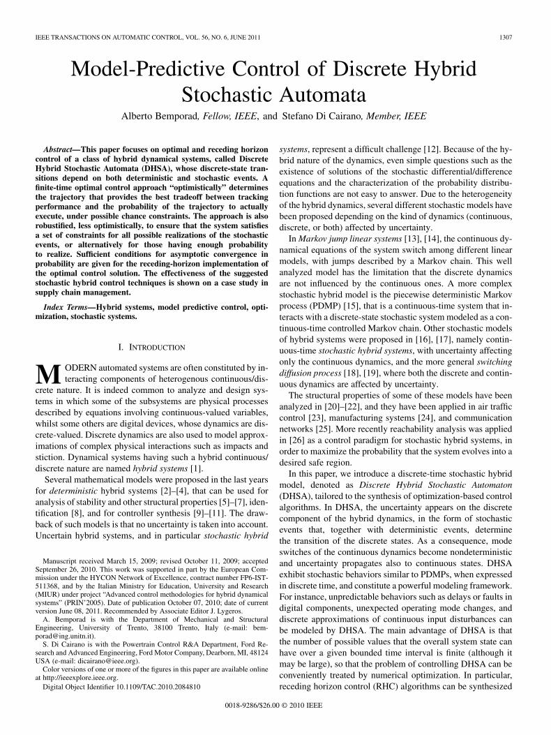
A DHSA is composed by the four components shown inFig. 1: the switched affine system, the event generator, thestochastic (nondeterministic) finite state machine, and themode selector. The switched affine system satisfies the lineardifference equations

(1)

in which is the discrete-time index,is the current mode of the system,

and are the vectors of continuousstates and continuous exogenous inputs, respectively, at time ,and , are constant matrices of suitable dimen-sions1. The event generator produces endogenous binary eventsignals defined by

(2)

where is the event generation func-tion defined as

where , , are con-stant matrices defining linear threshold conditions, and the su-

1Equation (1) can be extended with an output equation � �� , � � , where � �� areconstant matrices [38].

Fig. 1. Discrete hybrid stochastic automaton (DHSA). The superscript de-notes the successor at time � � �.

perscript denotes the -th row. The mode selector is definedby the Boolean function

(3)

where is the vector of binary states andis the vector of exogenous binary inputs. In (3) we

assume a “one-hot” encoding of the discrete state, hence, where , , is the unitary vector

of . As a consequence, is the number of the discrete-statevalues of the system.

Elements (1), (2), and (3) are the same as in DHA2. However,while in DHA the discrete dynamics are defined by the finitestate machine (FSM)

(4)

where is a Boolean func-tion defining the unique successor of the current state, in DHSAthey are defined by the stochastic FSM (sFSM)

(5)

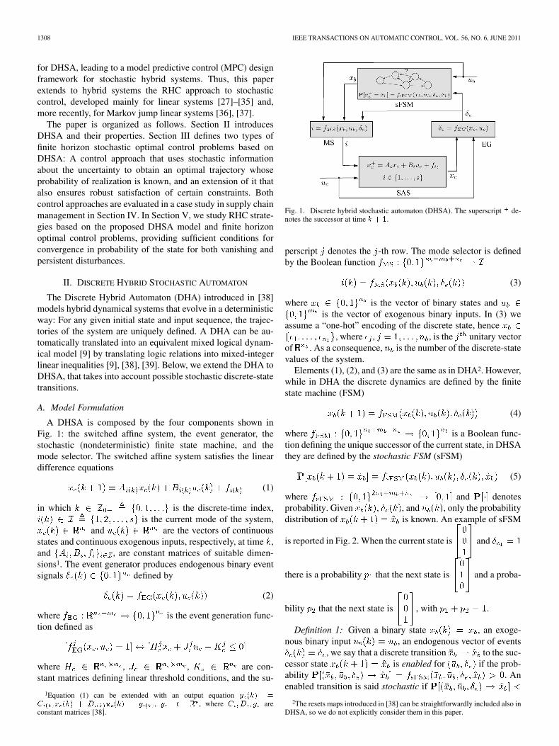
where and denotesprobability. Given , , and , only the probabilitydistribution of is known. An example of sFSM

is reported in Fig. 2. When the current state is and

there is a probability that the next state is and a proba-

bility that the next state is , with .

Definition 1: Given a binary state , an exoge-nous binary input , an endogenous vector of events

, we say that a discrete transition to the suc-cessor state is enabled for if the prob-ability . Anenabled transition is said stochastic if

2The resets maps introduced in [38] can be straightforwardly included also inDHSA, so we do not explicitly consider them in this paper.

BEMPORAD AND DI CAIRANO: MODEL-PREDICTIVE CONTROL OF DHSA 1309

Fig. 2. Example of stochastic finite state machine with three possible statevalues �� , �� , �� , two events � , � , and two stochastic tran-sitions with probabilities � , � � �� enabled in �� .

. Two or more transitions that are enabled for arecalled conflicting on .

Definition 2: An sFSM (5) is stochastically well-posed if, for all

.In order to demonstrate how a complex system can be mod-

elled as a DHSA, we briefly introduce a supply chain case study,that will be discussed in details in Section IV. In a supply chaincomposed of production, storage, and retailer nodes, the accu-mulation of products in the inventories and of wear in the ma-chines can be described by real-valued dynamics. The invento-ries are constrained by the storage capacity and when the ma-chine wear increases above a danger threshold, breakdowns,that disrupt the production capability, are possible with a cer-tain probability. The DHSA model of this system represents thereal-valued wear and inventory dynamics by the SAS, the activa-tion of the dangerous wear threshold by the EG, and the currentcondition of the production machines by the sFSM, whose stateindicates whether a machine is working, risking breakdown, orbroken. The MS is used to select the wear accumulation and theproduction dynamics according to the state of the sFSM.

B. Reformulation of DHSA as DHA With UncontrollableEvents (ueDHA)

A more explicit characterization of the uncertainty affectingthe DHSA (1), (2), (3), (5) is needed for use in numerical op-timization algorithms. The key idea is that an sFSM (5) having

stochastic transitions can be equivalently represented byan FSM (4) by introducing a random binary input ,called uncontrollable event, for each transition .The enabled stochastic transition occursif and only if a , with

(6)Let be associated with deterministic transitions,that is, whenever a transition from a binary state toanother is deterministic, or, equivalently, no conflicting (sto-chastic) transitions exist. Given any

, let de-note the subset of indices of the uncontrollable events associ-ated with the conflicting transitions on .

Let be the set of vectorsthat satisfy the condition

(7a)

(7b)

(7c)

Equation (7) imposes that: (i) when enabled conflicting tran-sitions exist (i.e., ), then oneand only one transition is taken ( ); (ii) if

then the corresponding tran-sition is deterministic, and in this case we assume withoutloss of generality that all deterministic transitions are as-sociated with , i.e., ; when

no transition is defined (the system“hangs” at that particular discrete state). As an example, thesFSM represented in Fig. 2 can be associated with a FSM havingadditional uncontrollable events that affect

the stochastic transitions in : transition

happens when is true (“ ” denotes logic “and”),

while transition when is true,

and satisfy ,

, and . Condition(7c) does not directly affect the evolution of the system, sincethe transitions that are not in the set arenot enabled and the value of the corresponding uncontrollableevents does not affect the discrete state evolution. However,(7c) is enforced to correctly compute the transition probability.

More generally, an sFSM having stochastic transitionscan be transformed into a deterministic automaton, denoted asFSM with uncontrollable-events (ueFSM), defined by

(8)

where is the random vectorof uncontrollable events at time ,

is derived from (5), and from now is a shortnotation for . The following propositionis immediate to prove.

Proposition 1: An sFSM (5) is stochastically well posed ifand only if the components of in its equivalentueFSM (8) are produced by an IID random binary number gen-erator with probabilities , ,

, satisfying

(9)Note that in case of deterministic transitions (9) implies that

, which ensures that the only possible transition is alwaystaken.


The notion of equivalent ueDHA to a given DHSA is formallydefined below.

Definition 3: Given a DHSA (1), (2), (3), (5), its equivalentueDHA is defined by (1), (2), (3), (8) with vectors

satisfying (7) and generated according to (9).We extend the definition of well-posedness given for deter-

ministic hybrid systems in [40, Def. 1] to DHSA.Definition 4: A DHSA (1), (2), (3), (5) is well-posed if its

ueDHA equivalent is well-posed according to [40, Def. 1] as adeterministic DHA with inputs ,

and the components of have prob-abilities satisfying (9).

In the rest of the paper, we will assume that DHSA modelsare well-posed.

The ueDHA representation of the DHSA has two advantages.First, the uncertainty is associated with so to that the prob-ability of a state trajectory can be obtained as a function of thesequence of the corresponding uncontrollable events. Second,the ueDHA dynamics (1), (2), (3), (8) under the constraints (7)can be written in mixed logical dynamical (MLD) form as

(10a)

(10b)

where , , and ,are auxiliary vectors, whose value is uniquely assigned for anyfixed , , . The matrices in (10) are obtainedfrom (1), (2), (3), (8) by automated procedures [38].

Given ,, and ,

the probability of the state trajectory ,, can be computed as follows. Consider the vector

containing the probability coefficients of thetransitions and

......

(11)

Each term describes the probability of taking the transitiondefined by at step , the probability of the completetrajectory and hence, being defined by (6), of the completestate trajectory defined by for the given and .

C. Stochastic Mode Selector and Additive StochasticDisturbances

Uncontrollable events can be easily included also in the modeselector function (3)

(12)

where satisfies properties similar to (7), (9).

A stochastic mode selector (12) can be used to model additivestochastic quantized disturbances affecting the contin-uous dynamics. Consider the simplest case

(13)

with taking values in with probabilities, , and is a constant ma-

trix of suitable dimension. We introduce uncontrollableevents , , with the sameprobabilities , define the switched affine dynamics

, , , and define (12) as. The quantized disturbance can

be considered as a piecewise constant approximation of agiven continuous disturbance with probability distribution

, for instance by partitioning the domain of into cells, and defining , .

III. FINITE HORIZON STOCHASTIC OPTIMAL CONTROL

A finite-time optimal control problem for a discrete-time dy-namical system can always be reformulated as a finite-dimen-sional optimization problem, in which the optimization vectoris the sequence of control inputs and the constraintsembed conditions on inputs and states that must be satisfied,such as bounds on inputs and states. If the system is stochastic,a sequence of stochastic variables will also appear inthe optimization problem.

When stochastic optimization algorithms are used to optimizethe expected value of the performance criterion, usually a “sce-nario enumeration” approach is employed [41]. This amountsto consider a discrete set of disturbances and to explicitly enu-merate all of them in the optimization problem. However, whenthe optimal control horizon gets large, the problem becomeseasily intractable as the number of scenarios grows exponen-tially. Scenario enumeration can be applied to DHSA by enu-merating the realizations of . However, the exponentialgrowth of the number of scenarios will affect the DHSA as well(see the discussion at the end of Section III-A).

For the above reason, in this paper we avoid minimizingaverage performance and consider instead the problem ofchoosing the input profile that optimizes the most favorable sit-uation, under penalties and hard constraints on the probabilityof the disturbance realization that determines such a favorablesituation. Such an “optimistic” approach is detailed next.

A. Finite Horizon Optimal Control Setup

Consider the convex performance indexdefined as

(14)

where for DHSA ,are reference signals for state ( ) and input ( ) trajecto-ries3, and we assumethat , for all references .

3References on output trajectories can also be included similarly.


Typical example of the stage cost that satisfy such assump-tions arewhere are full rank matrices, or

where ,are positive (semi)definite matrices.

Next, consider the probability cost defined as

(15)

The smaller the probability of a disturbance realization ,the larger is the probability cost, so that trajectories that realizerarely are penalized. The most desirable situation is to obtaina trajectory with high performance (small ) and high proba-bility (small ). Hence, we define as objective function

(16)

where , and is theprobability weight trading off between optimism (performance)and realism (chance, i.e., likelihood of the predicted trajectory).The coefficient must be greater than 0 to account for the prob-ability of the trajectory in (16), since as will be shown later, thisis important for convergence of the control algorithm.

In order to completely eliminate trajectories that realize rarelyfrom the set of feasible solutions, we also consider the chanceconstraint [27], [28], [34]

(17)

where is called probability bound. Chance constraint(17) enforces that , and hence the corresponding trajectory

, realizes with probability at least . More general constraintson could be imposed. The problem of optimally controlling aDHSA with respect to (16) subject to (17) is formulated throughits equivalent ueDHA.

1) Problem 1 (Stochastic Hybrid Optimal Control, SHOC):

(18a)

(18b)

(18c)

(18d)

where , are the sequence ofauxiliary vectors in (10), (18c) models constraints on the closed-loop system and the probabilities , , of satisfy(9).

In order to formulate (18) as a mixed-integer linear/quadraticprogram, we need to transform (15) and (17) into linear func-tions of . We assume that can be ex-pressed through mixed-integer linear inequalities [39] (see laterin (23)). can be dealt with as described in [42] for the deter-ministic case (see also (23)).

Consider a DHSA whose transition probabilities are collectedin vector , and consider the equivalent ueDHAwith uncontrollable events . By (11),

, where represents the contribution onthe trajectory probability of the stochastic transition at step ,

and is defined by

ifif .

(19)

Equivalently, . Hence

(20)

For all

Since for , , for all,

(21)

Thus, (20) is expressed as a linear function of , and (17) as alinear constraint on .

The solution of (18) is a pair , where is the op-timal control sequence for the predicted sequence of un-controllable events that respects all the dynamical and opera-tional constraints, the chance constraints, and that represents thebest tradeoff between performance and likelihood of the pre-dicted trajectory. Note that, since random event probabilities area function of the system state, dynamics prediction ( ) andcontrol action selection ( ) have to be performed together.

Since only can be decided and actuated, the trajectorymay be different from the one provided by (18), unless the re-alization of the stochastic events is equal to . The larger ,the more the prediction likelihood is important in the optimiza-tion problem, hence trajectories where more likely will co-incide with will be preferred, at the expense of a possiblydiminished performance. Chance constraint (17) ensures that

, or, in other words, that the actual state evo-lution of the system is different from the expected optimal onewith probability at most . The more restrictive is (17), themore trajectories are eliminated a priori, which may ease the so-lution of the optimization problem (18). However, if is set toolarge, many trajectories are eliminated by (17), and (18) may beinfeasible or result in poor performance (14).

Remark 1: while useful for notational purposes, for practicalpurposes , is removed from (1), since its contribution to (15)is always zero. Condition (7c) is also removed from (1), sinceif the transition associated with is not enabled, the value of

does not affect the trajectory, while setting causes anadditional cost. Thus, the optimal solution of (18) is guaranteedto have for all associated to nonenabled transitions.

As discussed in [9], in finite horizon optimal control of DHAthe optimizer of the associated mixed integer program is com-posed of the input vector , , . For Problem 1, the uncontrol-lable event vector is also included. Let , , , bethe size of those vectors, respectively, be the number of con-straints. The size of these vectors is indeed proportional to thehorizon . Along the horizon, the possible scenarios are ,


i.e., all the possible realizations of . Note that infeasible sce-nario pruning is not possible a priori, since the scenario realiza-tion depends on the control input, which is a decision variable.Thus, if a scenario enumeration approach is used for controllingthe DHSA, the size of the optimizer is ,and the number of constraints is . In fact, is fixedby the scenario, while and have to be duplicated for each sce-nario (since the logical expressions are possibly different), andthe constraints enforced for all scenarios. In the SHOC problemthere are variables and constraints,a much simpler problem than a scenario enumeration approachwould require.

B. Robust Constraint Handling

The SHOC approach does not ensure that constraints are sat-isfied when the actual disturbance realization differs from

. Henceforth, the SHOC approach can only be used when apossible violation of (18c) is not critical. On the other hand, forsafety critical constraints, it may be necessary to satisfy (18c)for any disturbance realization, or at least for disturbance real-izations having enough probability to happen.

Definition 5: Given a DHSA, an initial conditionand an input sequence , we say that a constraint

is robustly satisfied in probability if it is sat-isfied for all such that , . We saythat the constraint is robustly satisfied if , that is, if it issatisfied for all that can realize.

Problem (1) is extended to robustly satisfy constraint (18c).1) Problem 2 (Robustified SHOC, RSHOC):

(22a)

(22b)

(22c)

(22d)

(22e)

where . Compared to Problem 1, Problem 2 requiresin (22e) that the optimal input is such that constraint

is robustly satisfied for all the admissiblevalues of stochastic events that have a certain probability torealize (or all of them), while still optimizing the input sequence

and the predicted disturbance trajectory as in Problem 1.Note that in (17) is a lower bound on the probability of thecomputed optimal solution, while in (22e) defines an upperbound on the probability of the disturbance sequences againstwhich robust constraints are enforced.

By the techniques of Section III-A and of [9], (22) can beformulated as

(23a)

(23b)

(23c)

(23d)

(23e)

where is the predicted sequence of uncontrollableevents, is any other sequence of uncontrollable eventswith probability to realize greater than , (23a)–(23b) are thereformulation of the performance index (22a) and of the dy-namics (22b), (23c) is the mixed-integer equivalent reformula-tion of constraint (18c), and (23e) the reformulation of (22c).For simplicity of notation, (resp., ) collects and as-sociated4 to the DHSA dynamics evolving from by and

(resp., ).Because of the quantified constraints (23e), (23) cannot be di-

rectly formulated as a mixed integer program. As the possiblevalues of are finite, it would be possible to ex-pand the quantified constraints in groups of normal constraints,one for each realization of , as in scenario enumera-tion. However, as observed earlier, the obtained mixed-integerproblem would be intractable in most practical cases.

In general, only certain sequences lead to constraint vio-lation for a fixed . We propose a procedure to enumerateonly such potentially dangerous sequences . The procedureis based on the interaction between a “partially” robustly con-strained optimal control problem to get a candidate solution ,and a reachability problem aiming at determining whether anevent sequence with probability larger than existsthat violates (18c), for the given and control input

. Such a reachability problem is solved by the mixed-integerfeasibility program

(24a)

(24b)

(24c)

(24d)

where represent the logical “or” and denotes the -th com-ponent of function . When is a (mixed in-teger) linear inequality in , , , (24d) can be expressedthrough mixed logical/linear inequalities by associating to each

a binary variable (whichcan be transformed to mixed integer linear inequalities by usingfor instance the big-M technique [39]) and by introducing theconstraint . If (24) is infeasible, then constraint(23e) is satisfied. On the other hand, any feasible solution of(24) provides a counterexample to (23e). Further trajectoriesviolating (23e) can be iteratively found (if they exist) by simplyadding the “no good” cut in problem (24) [44].

4In case infinity norms are used in the performance index � , � also includesadditional variables required to carry on the optimization, and an additional termlinear in � needs to be added in (23b), and�� [43]; when quadratic forms[9] are used, � � �.


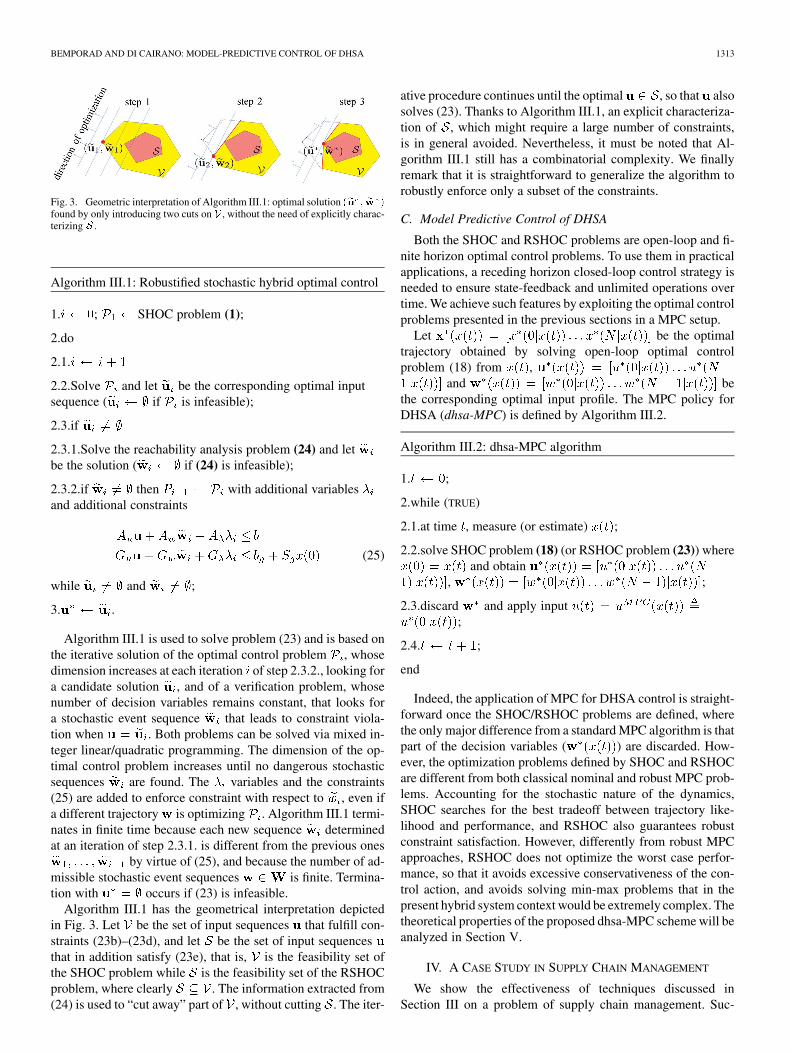
Fig. 3. Geometric interpretation of Algorithm III.1: optimal solution �� found by only introducing two cuts on � , without the need of explicitly charac-terizing � .

Algorithm III.1: Robustified stochastic hybrid optimal control

1. ; SHOC problem (1);

2.do

2.1.

2.2.Solve and let be the corresponding optimal inputsequence ( if is infeasible);

2.3.if

2.3.1.Solve the reachability analysis problem (24) and letbe the solution ( if (24) is infeasible);

2.3.2.if then with additional variablesand additional constraints

(25)

while and ;

3. .

Algorithm III.1 is used to solve problem (23) and is based onthe iterative solution of the optimal control problem , whosedimension increases at each iteration of step 2.3.2., looking fora candidate solution , and of a verification problem, whosenumber of decision variables remains constant, that looks fora stochastic event sequence that leads to constraint viola-tion when . Both problems can be solved via mixed in-teger linear/quadratic programming. The dimension of the op-timal control problem increases until no dangerous stochasticsequences are found. The variables and the constraints(25) are added to enforce constraint with respect to , even ifa different trajectory is optimizing . Algorithm III.1 termi-nates in finite time because each new sequence determinedat an iteration of step 2.3.1. is different from the previous ones

by virtue of (25), and because the number of ad-missible stochastic event sequences is finite. Termina-tion with occurs if (23) is infeasible.

Algorithm III.1 has the geometrical interpretation depictedin Fig. 3. Let be the set of input sequences that fulfill con-straints (23b)–(23d), and let be the set of input sequencesthat in addition satisfy (23e), that is, is the feasibility set ofthe SHOC problem while is the feasibility set of the RSHOCproblem, where clearly . The information extracted from(24) is used to “cut away” part of , without cutting . The iter-

ative procedure continues until the optimal , so that alsosolves (23). Thanks to Algorithm III.1, an explicit characteriza-tion of , which might require a large number of constraints,is in general avoided. Nevertheless, it must be noted that Al-gorithm III.1 still has a combinatorial complexity. We finallyremark that it is straightforward to generalize the algorithm torobustly enforce only a subset of the constraints.

C. Model Predictive Control of DHSA

Both the SHOC and RSHOC problems are open-loop and fi-nite horizon optimal control problems. To use them in practicalapplications, a receding horizon closed-loop control strategy isneeded to ensure state-feedback and unlimited operations overtime. We achieve such features by exploiting the optimal controlproblems presented in the previous sections in a MPC setup.

Let be the optimaltrajectory obtained by solving open-loop optimal controlproblem (18) from ,

and bethe corresponding optimal input profile. The MPC policy forDHSA (dhsa-MPC) is defined by Algorithm III.2.

Algorithm III.2: dhsa-MPC algorithm

1. ;

2.while (TRUE)

2.1.at time , measure (or estimate) ;

2.2.solve SHOC problem (18) (or RSHOC problem (23)) whereand obtain

, ;

2.3.discard and apply input;

2.4. ;

end

Indeed, the application of MPC for DHSA control is straight-forward once the SHOC/RSHOC problems are defined, wherethe only major difference from a standard MPC algorithm is thatpart of the decision variables ( ) are discarded. How-ever, the optimization problems defined by SHOC and RSHOCare different from both classical nominal and robust MPC prob-lems. Accounting for the stochastic nature of the dynamics,SHOC searches for the best tradeoff between trajectory like-lihood and performance, and RSHOC also guarantees robustconstraint satisfaction. However, differently from robust MPCapproaches, RSHOC does not optimize the worst case perfor-mance, so that it avoids excessive conservativeness of the con-trol action, and avoids solving min-max problems that in thepresent hybrid system context would be extremely complex. Thetheoretical properties of the proposed dhsa-MPC scheme will beanalyzed in Section V.

IV. A CASE STUDY IN SUPPLY CHAIN MANAGEMENT

We show the effectiveness of techniques discussed inSection III on a problem of supply chain management. Suc-


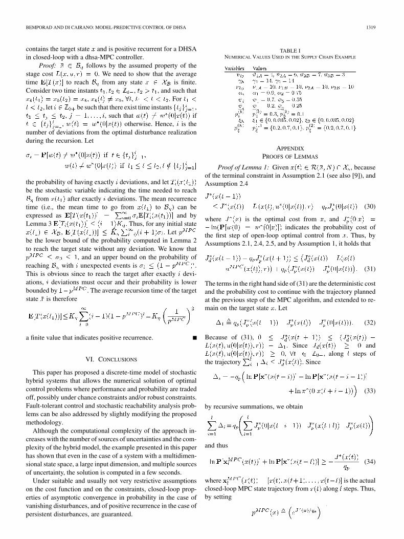
cessful examples of optimization-based control of supplychains exist in the literature, see for instance [45]. We considera supply chain that distributes two product types , , and thatis composed of three production nodes , , twostorage nodes , , and one retailer node . Theproducts are fractionable, i.e., their quantities are measured byreal numbers. During each control step, any can produce atmost one type of products in a fixed quantity , ,and ship it to one storage node only. Also, can produce onlytype , only type , while both types. Moreover, a per-centage of the items of type shipped from each storage nodeto the supplier may be returned to the corresponding storagenode. The percentage of shipped items from that is returned isrepresented as a discrete stochastic disturbance where

is a discrete set with cardinality , and for each ,, is the corresponding probability.

The storage nodes provide the supplier with the requestedamount of products to be sold, so that the dynamics of theproduct stored at node is

(26a)

(26b)

where if and only if producer is producing and ship-ping type to storage , ,

, and are the amount of product of type sent fromstorage to the retailer, and coefficients , .Each storage node stores products of both types and hasa limited storage space , where the occupation of producttypes is considered to be the same and normalized to 1. Hence,

. Similarly, the products of type providedfrom to are limited by , hence . The ob-jective of the supply chain planning system is to meet as muchas possible the product demands of products type and at theretailer, , respectively, that is to haveas close as possible to , . Note that the demandcan be exceeded, a situation which is not desirable since casethe retailer is forced to remove the excess products by tradingthem at low price.

In addition, and accumulate wear when producing. Thewear dynamics is described by

(27)

where , , is a coefficient related to mainte-nance frequency. When the wear level there is a proba-bility that breaks. When this happens, cannot produceanymore until its wear crosses the lower threshold .

The system is modelled as a DHSA with six continuous states(the products at the storage nodes , , ,and the producers’ wear , ), eight binary inputs(the allowed producer-to-storage node-shipping paths ), andfour continuous input variables (the quantities , providedfrom the storage nodes to the retailer).

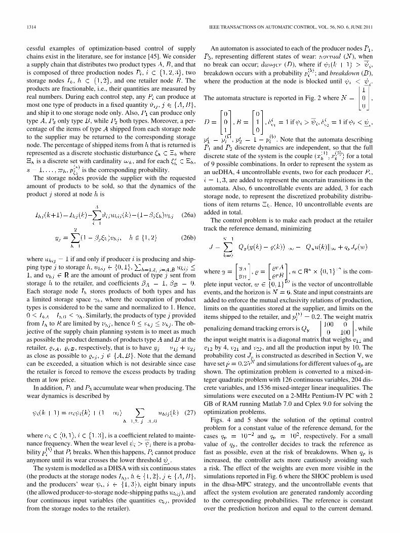
An automaton is associated to each of the producer nodes ,, representing different states of wear: ( ), when

no break can occur; ( ), where if ,breakdown occurs with a probability ; and breakdown ( ),where the production at the node is blocked until .

The automata structure is reported in Fig. 2 where ,

, , if , if ,

, . Note that the automata describingand discrete dynamics are independent, so that the full

discrete state of the system is the couple for a totalof 9 possible combinations. In order to represent the system asan ueDHA, 4 uncontrollable events, two for each producer ,

, are added to represent the uncertain transitions in theautomata. Also, 6 uncontrollable events are added, 3 for eachstorage node, to represent the discretized probability distribu-tions of item returns . Hence, 10 uncontrollable events areadded in total.

The control problem is to make each product at the retailertrack the reference demand, minimizing

where , , is the com-

plete input vector, is the vector of uncontrollableevents, and the horizon is . State and input constraints areadded to enforce the mutual exclusivity relations of production,limits on the quantities stored at the supplier, and limits on theitems shipped to the retailer, and . The weight matrix

penalizing demand tracking errors is , while

the input weight matrix is a diagonal matrix that weighs andby 4, and , and all the production input by 10. The

probability cost is constructed as described in Section V, wehave set and simulations for different values of areshown. The optimization problem is converted to a mixed-in-teger quadratic problem with 126 continuous variables, 204 dis-crete variables, and 1536 mixed-integer linear inequalities. Thesimulations were executed on a 2-MHz Pentium-IV PC with 2GB of RAM running Matlab 7.0 and Cplex 9.0 for solving theoptimization problems.

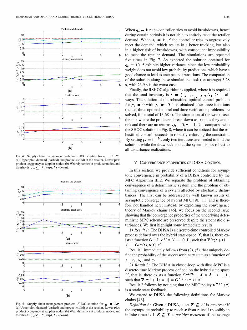
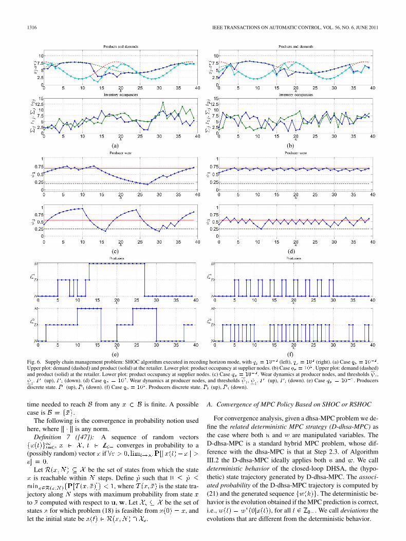
Figs. 4 and 5 show the solution of the optimal controlproblem for a constant value of the reference demand, for thecases and , respectively. For a smallvalue of , the controller decides to track the reference asfast as possible, even at the risk of breakdowns. When isincreased, the controller acts more cautiously avoiding sucha risk. The effect of the weights are even more visible in thesimulations reported in Fig. 6 where the SHOC problem is usedin the dhsa-MPC strategy, and the uncontrollable events thataffect the system evolution are generated randomly accordingto the corresponding probabilities. The reference is constantover the prediction horizon and equal to the current demand.


Fig. 4. Supply chain management problem: SHOC solution for � � �� .(a) Upper plot: demand (dashed) and product (solid) at the retailer. Lower plot:product occupancy at supplier nodes. (b) Wear dynamics at producer nodes, andthresholds � , � . � (up), � (down).

Fig. 5. Supply chain management problem: SHOC solution for � � �� .(a) Upper plot: demand (dashed) and product (solid) at the retailer. Lower plot:product occupancy at supplier nodes. (b) Wear dynamics at producer nodes, andthresholds � , � . � (up), � (down).

When the controller tries to avoid breakdowns, henceduring certain periods it is not able to entirely meet the retailerdemand. When the controller tries to aggressivelymeet the demand, which results in a better tracking, but alsoin a higher risk of breakdowns, with consequent impossibilityto meet the retailer demand. The simulations are repeatedfive times in Fig. 7. As expected the solution obtained for

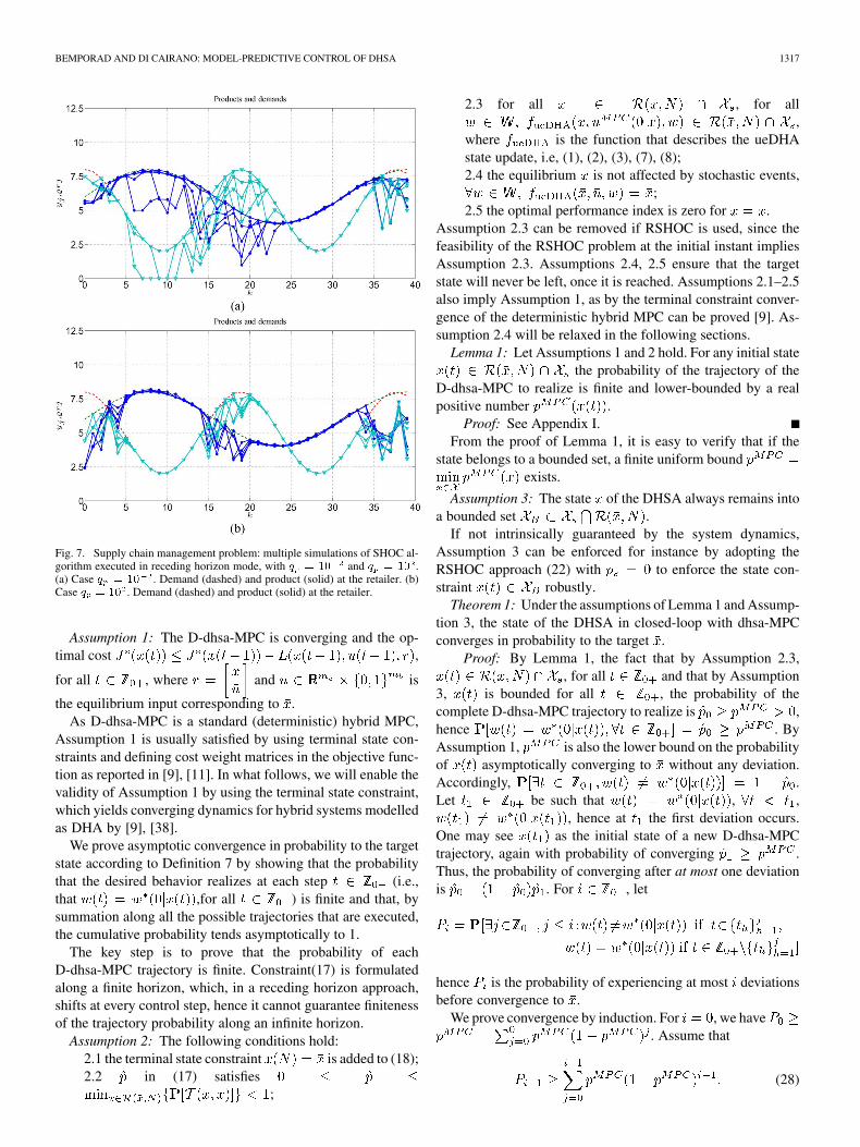
exhibits higher variance, since the low probabilityweight does not avoid low probability predictions, which have agood chance to lead to unexpected transitions. The computationof the solution along these simulations took (on average) 3.28s, with 23.9 s is the worst case.

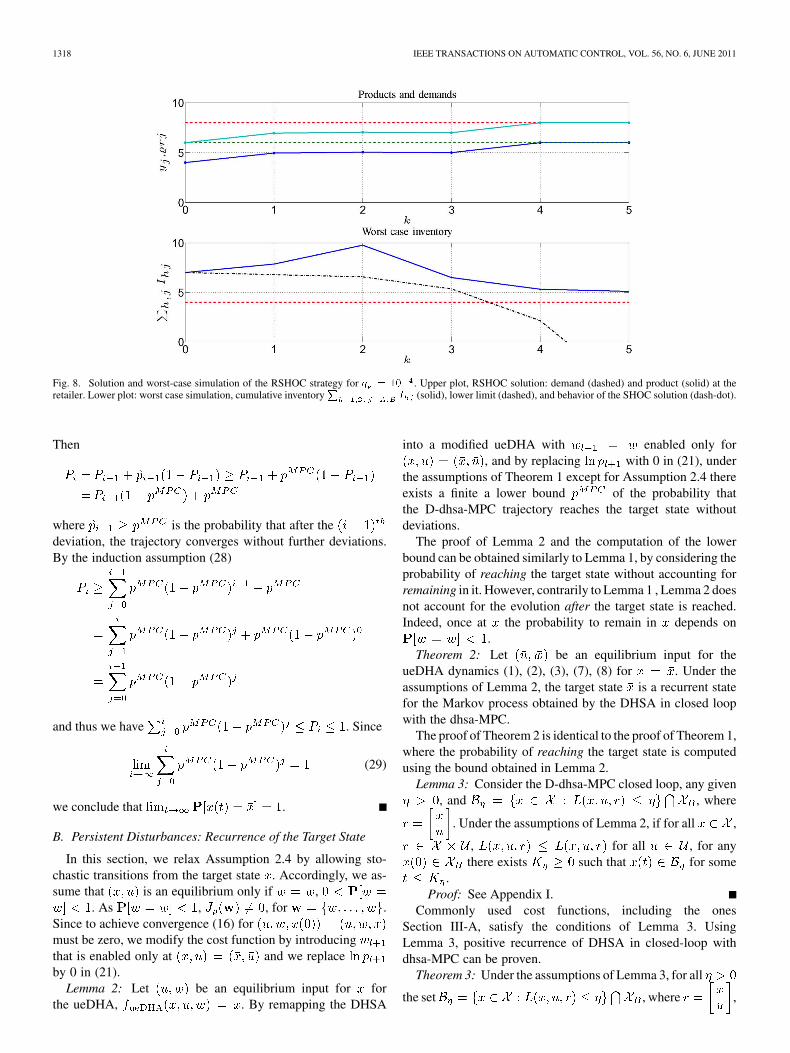
Finally, the RSHOC algorithm is applied, where it is requiredthat the total inventory is , al-ways. The solution of the robustified optimal control problemfor with is obtained after three iterations(hence, three optimal control and three verification problems aresolved, for a total of 13.68 s). The simulation of the worst case,the one where the producers break down as soon as they are atrisk and there are no returns, , , is compared withthe SHOC solution in Fig. 8, where it can be noticed that the ro-bustified control succeeds in robustly enforcing the constraint.By setting , only two iterations are needed to find thesolution, while the drawback is that the system is not robust toall disturbance realizations.

V. CONVERGENCE PROPERTIES OF DHSA CONTROL

In this section, we provide sufficient conditions for asymp-totic convergence in probability of a DHSA controlled by theMPC Algorithm III.2. We separate the problem of obtainingconvergence of a deterministic system and the problem of ob-taining convergence of a system affected by stochastic distur-bances. The first can be addressed by well known results ofasymptotic convergence of hybrid MPC [9], [11] and is there-fore not handled here. Instead, by exploiting the convergencetheory of Markov chains [46], we focus on the second issueshowing that the convergence properties of the underlying deter-ministic MPC scheme are preserved despite the stochastic dis-turbances. We first highlight some immediate results.

1) Result 1: The DHSA is a discrete-time controlled Markovprocess defined over the hybrid state-space , that is, there ex-ists a function , such that

.Result 1 immediately follows from (2), (5), that uniquely de-

fine the probability of the successor binary state as a function of, , , and .2) Result 2: The DHSA in closed-loop with dhsa-MPC is a

discrete-time Markov process defined on the hybrid state space, that is, there exists a function ,

such that .Result 2 follows by noticing that the MPC policy

is a static state feedback.We extend to DHSA the following definitions for Markov

chains [46].Definition 6: Given a DHSA, a set is recurrent if

the asymptotic probability to reach from itself (possibly ininfinite time) is 1. is positive recurrent if the average


Fig. 6. Supply chain management problem: SHOC algorithm executed in receding horizon mode, with � � �� (left), � � �� (right). (a) Case � � �� .Upper plot: demand (dashed) and product (solid) at the retailer. Lower plot: product occupancy at supplier nodes. (b) Case � � �� . Upper plot: demand (dashed)and product (solid) at the retailer. Lower plot: product occupancy at supplier nodes. (c) Case � � �� . Wear dynamics at producer nodes, and thresholds � ,� . � (up), � (down). (d) Case � � �� . Wear dynamics at producer nodes, and thresholds � , � . � (up), � (down). (e) Case � � �� . Producersdiscrete state. � (up), � (down). (f) Case � � �� . Producers discrete state. � (up), � (down).

time needed to reach from any is finite. A possiblecase is .

The following is the convergence in probability notion usedhere, where is any norm.

Definition 7 ([47]): A sequence of random vectors, , converges in probability to a

(possibly random) vector if.

Let be the set of states from which the stateis reachable within steps. Define such that

, where is the state tra-jectory along steps with maximum probability from stateto computed with respect to , . Let be the set ofstates for which problem (18) is feasible from , andlet the initial state be .

A. Convergence of MPC Policy Based on SHOC or RSHOC

For convergence analysis, given a dhsa-MPC problem we de-fine the related deterministic MPC strategy (D-dhsa-MPC) asthe case where both and are manipulated variables. TheD-dhsa-MPC is a standard hybrid MPC problem, whose dif-ference with the dhsa-MPC is that at Step 2.3. of AlgorithmIII.2 the D-dhsa-MPC ideally applies both and . We calldeterministic behavior of the closed-loop DHSA, the (hypo-thetic) state trajectory generated by D-dhsa-MPC. The associ-ated probability of the D-dhsa-MPC trajectory is computed by(21) and the generated sequence . The deterministic be-havior is the evolution obtained if the MPC prediction is correct,i.e., , for all . We call deviations theevolutions that are different from the deterministic behavior.


Fig. 7. Supply chain management problem: multiple simulations of SHOC al-gorithm executed in receding horizon mode, with � � �� and � � �� .(a) Case � � �� . Demand (dashed) and product (solid) at the retailer. (b)Case � � �� . Demand (dashed) and product (solid) at the retailer.

Assumption 1: The D-dhsa-MPC is converging and the op-timal cost ,

for all , where and is

the equilibrium input corresponding to .As D-dhsa-MPC is a standard (deterministic) hybrid MPC,

Assumption 1 is usually satisfied by using terminal state con-straints and defining cost weight matrices in the objective func-tion as reported in [9], [11]. In what follows, we will enable thevalidity of Assumption 1 by using the terminal state constraint,which yields converging dynamics for hybrid systems modelledas DHA by [9], [38].

We prove asymptotic convergence in probability to the targetstate according to Definition 7 by showing that the probabilitythat the desired behavior realizes at each step (i.e.,that ,for all ) is finite and that, bysummation along all the possible trajectories that are executed,the cumulative probability tends asymptotically to 1.

The key step is to prove that the probability of eachD-dhsa-MPC trajectory is finite. Constraint(17) is formulatedalong a finite horizon, which, in a receding horizon approach,shifts at every control step, hence it cannot guarantee finitenessof the trajectory probability along an infinite horizon.

Assumption 2: The following conditions hold:2.1 the terminal state constraint is added to (18);2.2 in (17) satisfies

;

2.3 for all , for all,

where is the function that describes the ueDHAstate update, i.e, (1), (2), (3), (7), (8);2.4 the equilibrium is not affected by stochastic events,

;2.5 the optimal performance index is zero for .

Assumption 2.3 can be removed if RSHOC is used, since thefeasibility of the RSHOC problem at the initial instant impliesAssumption 2.3. Assumptions 2.4, 2.5 ensure that the targetstate will never be left, once it is reached. Assumptions 2.1–2.5also imply Assumption 1, as by the terminal constraint conver-gence of the deterministic hybrid MPC can be proved [9]. As-sumption 2.4 will be relaxed in the following sections.

Lemma 1: Let Assumptions 1 and 2 hold. For any initial statethe probability of the trajectory of the

D-dhsa-MPC to realize is finite and lower-bounded by a realpositive number .

Proof: See Appendix I.From the proof of Lemma 1, it is easy to verify that if the

state belongs to a bounded set, a finite uniform boundexists.

Assumption 3: The state of the DHSA always remains intoa bounded set .

If not intrinsically guaranteed by the system dynamics,Assumption 3 can be enforced for instance by adopting theRSHOC approach (22) with to enforce the state con-straint robustly.

Theorem 1: Under the assumptions of Lemma 1 and Assump-tion 3, the state of the DHSA in closed-loop with dhsa-MPCconverges in probability to the target .

Proof: By Lemma 1, the fact that by Assumption 2.3,, for all and that by Assumption

3, is bounded for all , the probability of thecomplete D-dhsa-MPC trajectory to realize is ,hence . ByAssumption 1, is also the lower bound on the probabilityof asymptotically converging to without any deviation.Accordingly, .Let be such that , ,

, hence at the first deviation occurs.One may see as the initial state of a new D-dhsa-MPCtrajectory, again with probability of converging .Thus, the probability of converging after at most one deviationis . For , let

hence is the probability of experiencing at most deviationsbefore convergence to .

We prove convergence by induction. For , we have. Assume that

(28)


Fig. 8. Solution and worst-case simulation of the RSHOC strategy for � � �� . Upper plot, RSHOC solution: demand (dashed) and product (solid) at theretailer. Lower plot: worst case simulation, cumulative inventory � (solid), lower limit (dashed), and behavior of the SHOC solution (dash-dot).

Then

where is the probability that after thedeviation, the trajectory converges without further deviations.By the induction assumption (28)

and thus we have . Since

(29)

we conclude that .

B. Persistent Disturbances: Recurrence of the Target State

In this section, we relax Assumption 2.4 by allowing sto-chastic transitions from the target state . Accordingly, we as-sume that is an equilibrium only if ,

. As , , for .Since to achieve convergence (16) formust be zero, we modify the cost function by introducingthat is enabled only at and we replaceby 0 in (21).

Lemma 2: Let be an equilibrium input for forthe ueDHA, . By remapping the DHSA

into a modified ueDHA with enabled only for, and by replacing with 0 in (21), under

the assumptions of Theorem 1 except for Assumption 2.4 thereexists a finite a lower bound of the probability thatthe D-dhsa-MPC trajectory reaches the target state withoutdeviations.

The proof of Lemma 2 and the computation of the lowerbound can be obtained similarly to Lemma 1, by considering theprobability of reaching the target state without accounting forremaining in it. However, contrarily to Lemma 1 , Lemma 2 doesnot account for the evolution after the target state is reached.Indeed, once at the probability to remain in depends on

.Theorem 2: Let be an equilibrium input for the

ueDHA dynamics (1), (2), (3), (7), (8) for . Under theassumptions of Lemma 2, the target state is a recurrent statefor the Markov process obtained by the DHSA in closed loopwith the dhsa-MPC.

The proof of Theorem 2 is identical to the proof of Theorem 1,where the probability of reaching the target state is computedusing the bound obtained in Lemma 2.

Lemma 3: Consider the D-dhsa-MPC closed loop, any given, and , where

. Under the assumptions of Lemma 2, if for all ,

, for all , for anythere exists such that for some

.Proof: See Appendix I.

Commonly used cost functions, including the onesSection III-A, satisfy the conditions of Lemma 3. UsingLemma 3, positive recurrence of DHSA in closed-loop withdhsa-MPC can be proven.

Theorem 3: Under the assumptions of Lemma 3, for all

the set , where ,


contains the target state and is positive recurrent for a DHSAin closed-loop with a dhsa-MPC controller.

Proof: follows by the assumed property of thestage cost . We need to show that the averagetime to reach from any state is finite.Consider two time instants , , and such that

, , , . For, let be such that there exist time instants ,

, , such that if, otherwise. Hence, is the

number of deviations from the optimal disturbance realizationduring the recursion. Let

the probability of having exactly deviations, and letbe the stochastic variable indicating the time needed to reach

from after exactly deviations. The mean recurrencetime (i.e., the mean time to go from to ) can beexpressed as and byLemma 3 . Thus, for any initial state

, . Letbe the lower bound of the probability computed in Lemma 2to reach the target state without any deviation. We know that

, and an upper bound on the probability ofreaching with unexpected events is .This is obvious since to reach the target after exactly devi-ations, deviations must occur and their probability is lowerbounded by . The average recursion time of the targetstate is therefore

a finite value that indicates positive recurrence.

VI. CONCLUSIONS

This paper has proposed a discrete-time model of stochastichybrid systems that allows the numerical solution of optimalcontrol problems where performance and probability are tradedoff, possibly under chance constraints and/or robust constraints.Fault-tolerant control and stochastic reachability analysis prob-lems can be also addressed by slightly modifying the proposedmethodology.

Although the computational complexity of the approach in-creases with the number of sources of uncertainties and the com-plexity of the hybrid model, the example presented in this paperhas shown that even in the case of a system with a multidimen-sional state space, a large input dimension, and multiple sourcesof uncertainty, the solution is computed in a few seconds.

Under suitable and usually not very restrictive assumptionson the cost function and on the constraints, closed-loop prop-erties of asymptotic convergence in probability in the case ofvanishing disturbances, and of positive recurrence in the case ofpersistent disturbances, are guaranteed.

TABLE INUMERICAL VALUES USED IN THE SUPPLY CHAIN EXAMPLE

APPENDIX

PROOFS OF LEMMAS

Proof of Lemma 1: Given , becauseof the terminal constraint in Assumption 2.1 (see also [9]), andAssumption 2.4

(30)

where is the optimal cost from , andindicates the probability cost of

the first step of open-loop optimal control from . Thus, byAssumptions 2.1, 2.4, 2.5, and by Assumption 1, it holds that

(31)

The terms in the right hand side of (31) are the deterministic costand the probability cost to continue with the trajectory plannedat the previous step of the MPC algorithm, and extended to re-main on the target state . Let

(32)

Because of (31),. Since and

, , along steps ofthe trajectory . Since

(33)

by recursive summations, we obtain

and thus

(34)

where is the actualclosed-loop MPC state trajectory from along steps. Thus,by setting


by (34) it follows that

(35)is finite and lower bounded. Hence, for the completeD-dhsa-MPC closed-loop trajectory, which by Assumption 1converges to the target state, has a finite probabilityto realize.

Proof of Lemma 3: By Assumption 3, the trajectory of theD-dhsa-MPC closed loop is such that , .Hence by the definition of , along the trajectories generatedby the D-dhsa-MPC control strategy, , ,and . Let be the initial state andassume by contradiction that for all , . By (30)

and therefore . Since is bounded,there exists a finite such that

Hence, ,which implies , a contradiction. By choosing

, where the maximum ex-ists because we are considering a bounded state-space, anddenotes roundoff to the smallest greater or equal integer, thelemma is proven.

REFERENCES

[1] P. Antsaklis, “A brief introduction to the theory and applications ofhybrid systems,” Proc. IEEE (Special Issue on Hybrid Systems: Theoryand Applications), vol. 88, no. 7, pp. 879–886, Jul. 2000.

[2] E. Sontag, “Nonlinear regulation: The piecewise linear approach,” IEEETrans. Autom. Control, vol. AC-26, no. 2, pp. 346–358, Apr. 1981.

[3] T. Henzinger, “The theory of hybrid automata,” in Proc. 11th Annu.IEEE Symp. Logic in Computer Science (LICS ’96), New Brunswick,NJ, 1996, pp. 278–292.

[4] W. Heemels, B. de Schutter, and A. Bemporad, “Equivalence of hybriddynamical models,” Automatica, vol. 37, no. 7, pp. 1085–1091, Jul.2001.

[5] A. Bemporad, G. Ferrari-Trecate, and M. Morari, “Observability andcontrollability of piecewise affine and hybrid systems,” IEEE Trans.Autom. Control, vol. 45, no. 10, pp. 1864–1876, Oct. 2000.

[6] M. Johannson and A. Rantzer, “Computation of piece-wise quadraticLyapunov functions for hybrid systems,” IEEE Trans. Autom. Control,vol. 43, no. 4, pp. 555–559, Apr. 1998.

[7] J. Lygeros, K. Johansson, S. Simic, J. Zhang, and S. Sastry, “Dynamicalproperties of hybrid automata,” IEEE Trans. Autom. Control, vol. 48,no. 1, pp. 2–17, Jan. 2003.

[8] A. Juloski, W. Heemels, G. Ferrari-Trecate, R. Vidal, S. Paoletti, and J.Niessen, “Comparison of four procedures for the identification of hy-brid systems,” Hybrid Syst.: Comput. and Control, pp. 354–369, 2005.

[9] A. Bemporad and M. Morari, “Control of systems integrating logic,dynamics, and constraints,” Automatica, vol. 35, no. 3, pp. 407–427,1999.

[10] F. Borrelli, M. Baotic, A. Bemporad, and M. Morari, “Dynamic pro-gramming for constrained optimal control of discrete-time linear hy-brid systems,” Automatica, vol. 41, no. 10, pp. 1709–1721, Oct. 2005.

[11] M. Lazar, W. Heemels, S. Weiland, and A. Bemporad, “Stabilizingmodel predictive control of hybrid systems,” IEEE Trans. Autom. Con-trol, vol. 51, no. 11, pp. 1813–1818, Nov. 2006.

[12] J. Lygeros, “Stochastic hybrid systems: Theory and applications,” inProc. 47th IEEE Conf. Decision and Control, 2008, pp. 40–42.

[13] E. Boukas and H. Yang, “Stability of discrete-time linear systems withMarkovian jumping parameters,” Mathemat. Control, Signals andSyst., vol. 8, pp. 390–402, 1995.

[14] P. Bolzern, P. Colaneri, and G. D. Nicolao, “On almost sure stability ofdiscrete-time Markov jump linear systems,” in Proc. 43th IEEE Conf.Decision and Control, Paradise Island, Bahamas, 2004, pp. 3204–3208.

[15] M. Davis, Markov Models and Optimization. London, U.K.:Chapman & Hall, 1993.

[16] G. Pola, M. Bujorianu, J. Lygeros, and M. Di Benedetto, “Stochastic hy-brid models: An overview with application to air traffic management,” inProc. IFAC Conf. Analysis and Design of Hybrid Systems, Apr. 2003.

[17] J. Hu, J. Lygeros, and S. Sastry, “Towards a theory of stochastic hybridsystems,” in Hybrid Systems: Computation and Control, B. Krogh andN. Lynch, Eds. New York: Springer-Verlag, 2000, vol. 1790, LectureNotes in Computer Science, pp. 160–173.

[18] M. Ghosh, A. Arapostathis, and S. Marcus, “Optimal control ofswitching diffusions with application to flexible manufacturing sys-tems,” SIAM J. Control and Optimiz., vol. 31, no. 5, pp. 1183–1204,1993.

[19] M. Ghosh, S. Marcus, and A. Arapostathis, “Controlled switching dif-fusions as hybrid processes,” in Hybrid Syst., G. Goos, R. Alur, andE. Sontag, Eds. : Springer-Verlag, 1996, vol. 1066, Lecture Notes inComputer Science, pp. 64–75.

[20] M. Bujorianu and J. Lygeros, “Reachability questions in piecewise de-terministic Markov processes,” in Hybrid Systems: Comput. and Con-trol, O. Maler and A. Pnueli, Eds. : Springer-Verlag, 2003, vol. 2623,Lecture Notes in Computer Science, pp. 126–140.

[21] D. Chatterjee and D. Liberzon, “On stability of randomly switchednonlinear systems,” IEEE Trans. Autom. Control, vol. 52, no. 12, pp.2390–2394, Dec. 2007.

[22] S. Strubbe, A. Julius, and A. van der Schaft, “Communicating piece-wise deterministic Markov processes,” in Proc. IFAC Conf. Analysisand Design of Hybrid Systems, 2003, pp. 349–354.

[23] M. Prandini, J. Hu, J. Lygeros, and S. Sastry, “A probabilistic approachto aircraft conflict detection,” IEEE Trans. Intell. Transport. Syst., vol.1, no. 4, pp. 199–220, Dec. 2000.

[24] C. Cassandras and R. Mookherjee, “Receding horizon optimal controlfor some stochastic hybrid systems,” in Proc. 41th IEEE Conf. Decisionand Control, 2003, pp. 2162–2167.

[25] J. Hespanha, “Stochastic hybrid systems: Application to communica-tion networks,” in Hybrid Syst.: Comput. and Control, R. Alur and G.Pappas, Eds. Berlin: Springer-Verlag, 2004, vol. 2993, Lecture Notesin Computer Science, pp. 387–401.

[26] A. Abate, M. Prandini, J. Lygeros, and S. Sastry, “Probabilistic reacha-bility and safety for controlled discrete time stochastic hybrid systems,”Automatica, vol. 44, no. 11, pp. 2724–2734, 2008.

[27] A. Schwarm and M. Nikolaou, “Chance-constrained model predictivecontrol,” AIChE J., vol. 45, no. 8, pp. 1743–1752, 1999.

[28] P. Li, M. Wendt, and G. Wozny, “Robust model predictive controlunder chance constraints,” Comput. and Chem. Eng., vol. 24, no. 2–7,pp. 829–834, 2000.

[29] D. van Hessem and O. Bosgra, “A conic reformulation of model predic-tive control including bounded and stochastic disturbances under stateand input constraints,” in Proc. 41th IEEE Conf. Decision and Control,Las Vegas, NV, 2002, pp. 4643–4648.

[30] I. Batina, A. Stoorvogel, and S. Weiland, “Optimal control of linear,stochastic systems with state and input constraints,” in Proc. 41th IEEEConf. on Decision and Control, 2002, vol. 2, pp. 1564–1569.

[31] D. Muñoz de la Peña, A. Bemporad, and T. Alamo, “Stochasticprogramming applied to model predictive control,” in Proc. 44th IEEEConf. Decision and Control and European Control Conf., Sevilla,Spain, 2005, pp. 1361–1366.

[32] P. Couchman, M. Cannon, and B. Kouvaritakis, “Stochastic MPC withinequality stability constraints,” Automatica, vol. 42, pp. 2169–2174,2006.

[33] J. Primbs and C. Sung, “Stochastic receding horizon control of con-strained linear systems with state and control multiplicative noise,”IEEE Trans. Autom. Control, vol. 54, no. 2, pp. 221–230, Feb. 2009.

[34] F. Oldewurtel, C. Jones, and M. Morari, “A tractable approximationof chance constrained stochastic MPC based on affine disturbancefeedback,” in Proc. 47th IEEE Conf. Decision and Control, Cancun,Mexico, 2008, pp. 4731–4736.

[35] P. Hokayem, D. Chatterjee, and J. Lygeros, “On stochastic recedinghorizon control with bounded control inputs,” in Proc. 48th IEEE Conf.Decision and Control, Shangai, China, 2009, pp. 6359–6364.

[36] L. Blackmore, A. Bektassov, M. Ono, and B. C. Williams, “Robustoptimal predictive control of jump Markov linear systems using parti-cles,” in Hybrid Syst.: Comput. and Control, A. Bemporad, A. Bicchi,and G. Buttazzo, Eds. New York: Springer-Verlag, 2007, vol. 4416,Lecture Notes in Computer Science, pp. 104–117.

[37] D. Bernardini and A. Bemporad, “Scenario-based model predictivecontrol of stochastic constrained linear systems,” in Proc. 48th IEEEConf. Decision and Control, 2009, pp. 6333–6338.


[38] F. Torrisi and A. Bemporad, “HYSDEL — A tool for generating com-putational hybrid models,” IEEE Trans. Control Syst. Technol., vol. 12,no. 2, pp. 235–249, Mar. 2004.

[39] H. Williams, Model Building in Mathematical Programming. NewYork: Wiley, 1993.

[40] A. Bemporad, W. Heemels, and B. D. Schutter, “On hybrid systemsand closed-loop MPC systems,” IEEE Trans. Autom. Control, vol. 47,no. 5, pp. 863–869, May 2002.

[41] J. Birge and F. Louveaux, Introduction to Stochastic Programming.New York: Springer, 1997.

[42] A. Bemporad, Hybrid Toolbox – User’s Guide 2003 [Online]. Avail-able: http://www.dii.unisi.it/hybrid/toolbox

[43] A. Bemporad, F. Borrelli, and M. Morari, “Piecewise linear optimalcontrollers for hybrid systems,” in Proc. American Control Conference,Chicago, IL, Jun. 2000, pp. 1190–1194.

[44] J. Hooker, Logic-Based Methods for Optimization: Combining Opti-mization and Constraint Satisfaction. New York: Wiley, 2000.

[45] J. Schwartz, W. Wang, and D. Rivera, “Simulation-based optimizationof process control policies for inventory management in supply chains,”Automatica, vol. 42, no. 8, pp. 1311–1320, 2006.

[46] C. G. Cassandras and S. Lafortune, Introduction to Discrete Event Sys-tems. Norwell, MA: Kluwer, 1999.

[47] A. Papoulis, Probability, Random Variables and Stochastic Pro-cesses. New York: McGraw-Hill, 1991.

Alberto Bemporad (S’95–M’99–SM’06–F’10) re-ceived the Master’s degree in electrical engineeringin 1993 and the Ph.D. degree in control engineeringin 1997 from the University of Florence, Florence,Italy.

He spent 1996–1997 at the Center for Roboticsand Automation, Department of Systems Scienceand Mathematics, Washington University, St. Louis,MO, as a Visiting Researcher. In 1997–1999, he helda postdoctoral position at the Automatic ControlLaboratory, ETH, Zurich, Switzerland, where he

collaborated as a Senior Researcher in 2000–2002. In 1999–2009, he was withthe Department of Information Engineering, University of Siena, Siena, Italy,becoming an Associate Professor in 2005. Since 2010, he has been with theDepartment of Mechanical and Structural Engineering, University of Trento,Trento, Italy. He has published more than 220 papers in the areas of modelpredictive control, hybrid systems, multiparametric optimization, computa-tional geometry, automotive control, robotics, and finance. He is coauthor ofthe Model Predictive Control Toolbox (The Mathworks, Inc.) and author of theHybrid Toolbox for Matlab.

Dr. Bemporad was an Associate Editor of the IEEE TRANSACTIONS ON

AUTOMATIC CONTROL during 2001–2004. He has been Chair of the TechnicalCommittee on Hybrid Systems of the IEEE Control Systems Society since2002.

Stefano Di Cairano (M’08) received the Laurea de-gree in computer engineering in 2004, and the Ph.D.degree in information engineering in 2008, both fromthe University of Siena, Siena, Italy. In 2008, he wasgranted the International Curriculum Option for Ph.S.studies in hybrid control for complex distributed andheterogenous embedded systems.

In 2002–2003, he was a Visiting Student at the In-formatics and Mathematical Modelling Department,Technical University of Denmark, Lyngby, Den-mark. In 2006–2007, he was a Visiting Researcher

at the Control and Dynamical Systems Department, California Institute ofTechnology, Pasadedna, CA, where he joined the team competing in the 2007DARPA Urban Challenge. In 2008, he joined the Powertrain Control Researchand Advanced Engineering Department, Ford Motor Company, Dearborn, MI,as a Sr. Research Engineer. His research focuses on the application of opti-mization-based control algorithms to complex systems including powertrain,vehicle dynamics, energy management, and supply chains. His interests includeautomotive control, model-predictive control, networked distributed controlsystems, hybrid systems, optimization algorithms, and stochastic control.

Documents

Model-Predictive Control of Discrete Hybrid Stochastic Automata