Embed Size (px)
Citation preview
Modeling television viewership
The Nielsen ratings are the best–known measures of viewership of television shows. These
ratings form the basis for the setting of advertising rates, and are thus crucial for the success
(and survival) of shows. The ratings, which are based on diaries kept by a sample of “Nielsen
families,” are intended to measure in–home viewing. This can result in biased figures for
shows that are often watched in large public areas such as bars or restaurants, such as sports
shows, or shows that appeal to people who watch television in groups, such as those aimed
at college–aged viewers.
Two ratings values are typically examined: the rating, which is (an estimate of) the
percentage of televisions tuned to a particular show at a particular time out of all televisions,
and the share, which is the percentage of televisions tuned to a particular show at a particular
time out of all televisions that are being used at that time. The latter variable corrects for
the fact that more or less television in general is watched on certain nights of the week.
These numbers can then be converted into estimates of the total number of viewers of the
program (and thereby total number of potential customers for the advertisers!).
The data analyzed here are the estimated household ratings for each of the 157 television
shows for new episodes during the 2011-2012 season (that is, not including repeat episodes
shown in the regular time slot). I am indebted to Karl Rosen for sharing these data with
me. For each show the network (ABC, CBS, CW, Fox, or NBC) and type (comedy, drama,
news, reality/participation, or animation) are recorded. Since these data are actually a
listing of all shows for 2011-2012, they are not a sample from that season, but rather should
be viewed as a “snapshot” sample from a (hopefully) stable ongoing process. That is, a
significant difference between two networks, for example, would hopefully say something
about the 2012-2013 season and beyond. Note that NBC’s “Sunday Night Football” and
ABC’s “Saturday Movie of the Week” are not included, since they were the only shows of
their type broadcast in prime time by the networks during the 2011-2012 season.
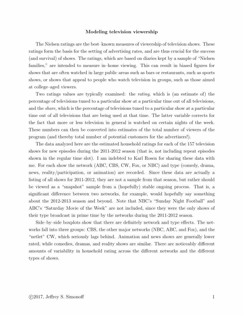
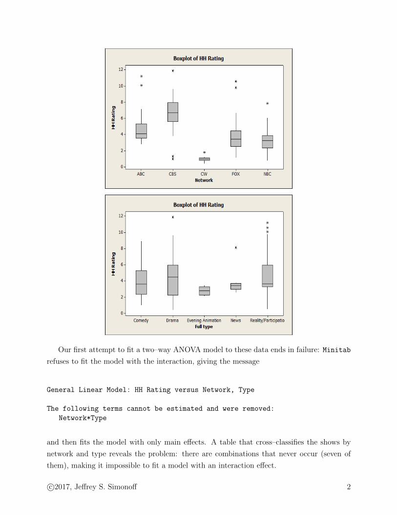
Side–by–side boxplots show that there are definitely network and type effects. The net-
works fall into three groups: CBS, the other major networks (NBC, ABC, and Fox), and the
“netlet” CW, which seriously lags behind. Animation and news shows are generally lower
rated, while comedies, dramas, and reality shows are similar. There are noticeably different
amounts of variability in household rating across the different networks and the different
types of shows.
c©2017, Jeffrey S. Simonoff 1
Our first attempt to fit a two–way ANOVA model to these data ends in failure: Minitab
refuses to fit the model with the interaction, giving the message
General Linear Model: HH Rating versus Network, Type
The following terms cannot be estimated and were removed:
Network*Type
and then fits the model with only main effects. A table that cross–classifies the shows by
network and type reveals the problem: there are combinations that never occur (seven of
them), making it impossible to fit a model with an interaction effect.
c©2017, Jeffrey S. Simonoff 2
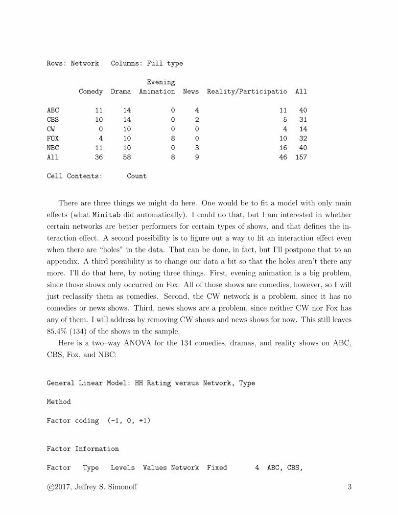
Rows: Network Columns: Full type
Evening
Comedy Drama Animation News Reality/Participatio All
ABC 11 14 0 4 11 40
CBS 10 14 0 2 5 31
CW 0 10 0 0 4 14
FOX 4 10 8 0 10 32
NBC 11 10 0 3 16 40
All 36 58 8 9 46 157
Cell Contents: Count
There are three things we might do here. One would be to fit a model with only main
effects (what Minitab did automatically). I could do that, but I am interested in whether
certain networks are better performers for certain types of shows, and that defines the in-
teraction effect. A second possibility is to figure out a way to fit an interaction effect even
when there are “holes” in the data. That can be done, in fact, but I’ll postpone that to an
appendix. A third possibility is to change our data a bit so that the holes aren’t there any
more. I’ll do that here, by noting three things. First, evening animation is a big problem,
since those shows only occurred on Fox. All of those shows are comedies, however, so I will
just reclassify them as comedies. Second, the CW network is a problem, since it has no
comedies or news shows. Third, news shows are a problem, since neither CW nor Fox has
any of them. I will address by removing CW shows and news shows for now. This still leaves
85.4% (134) of the shows in the sample.
Here is a two–way ANOVA for the 134 comedies, dramas, and reality shows on ABC,
CBS, Fox, and NBC:
General Linear Model: HH Rating versus Network, Type
Method
Factor coding (-1, 0, +1)
Factor Information
Factor Type Levels Values Network Fixed 4 ABC, CBS,
c©2017, Jeffrey S. Simonoff 3
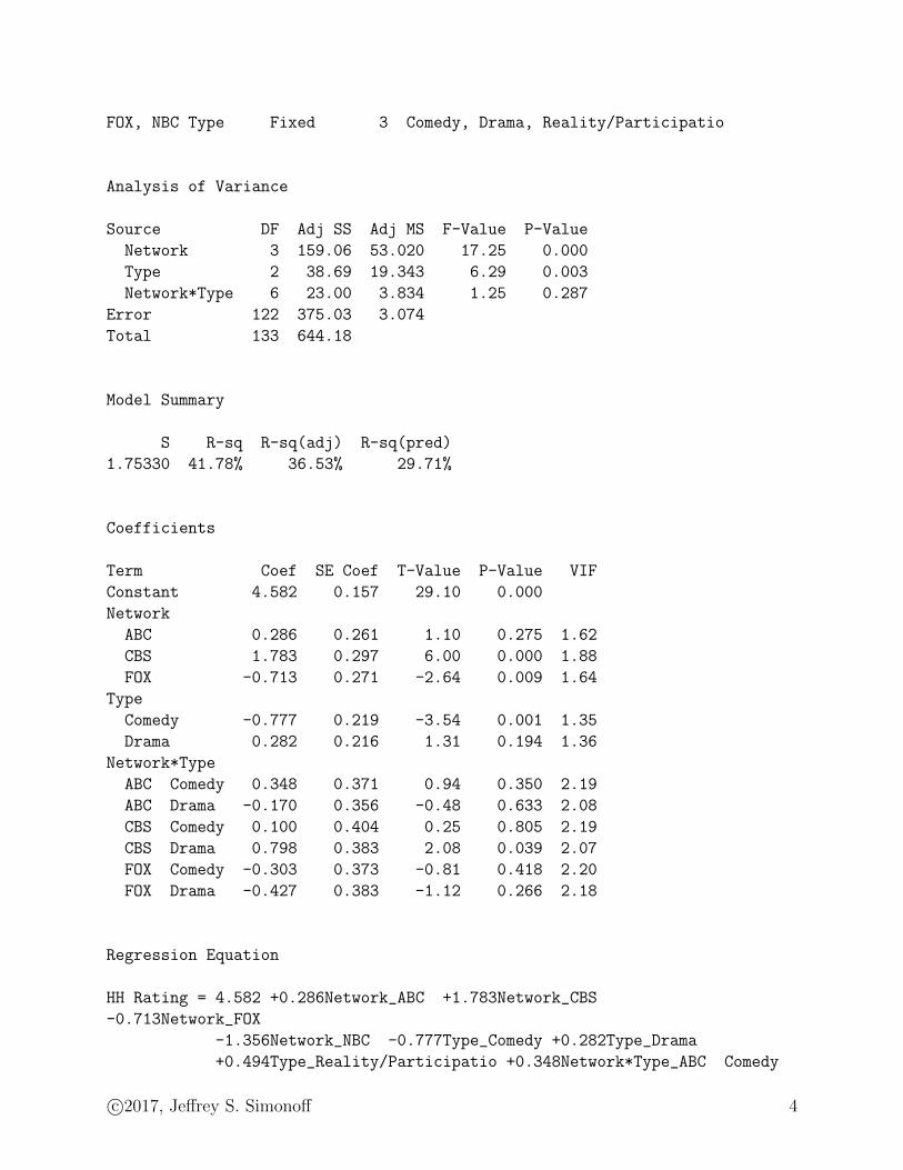
FOX, NBC Type Fixed 3 Comedy, Drama, Reality/Participatio
Analysis of Variance
Source DF Adj SS Adj MS F-Value P-Value
Network 3 159.06 53.020 17.25 0.000
Type 2 38.69 19.343 6.29 0.003
Network*Type 6 23.00 3.834 1.25 0.287
Error 122 375.03 3.074
Total 133 644.18
Model Summary
S R-sq R-sq(adj) R-sq(pred)
1.75330 41.78% 36.53% 29.71%
Coefficients
Term Coef SE Coef T-Value P-Value VIF
Constant 4.582 0.157 29.10 0.000
Network
ABC 0.286 0.261 1.10 0.275 1.62
CBS 1.783 0.297 6.00 0.000 1.88
FOX -0.713 0.271 -2.64 0.009 1.64
Type
Comedy -0.777 0.219 -3.54 0.001 1.35
Drama 0.282 0.216 1.31 0.194 1.36
Network*Type
ABC Comedy 0.348 0.371 0.94 0.350 2.19
ABC Drama -0.170 0.356 -0.48 0.633 2.08
CBS Comedy 0.100 0.404 0.25 0.805 2.19
CBS Drama 0.798 0.383 2.08 0.039 2.07
FOX Comedy -0.303 0.373 -0.81 0.418 2.20
FOX Drama -0.427 0.383 -1.12 0.266 2.18
Regression Equation
HH Rating = 4.582 +0.286Network_ABC +1.783Network_CBS
-0.713Network_FOX
-1.356Network_NBC -0.777Type_Comedy +0.282Type_Drama
+0.494Type_Reality/Participatio +0.348Network*Type_ABC Comedy
c©2017, Jeffrey S. Simonoff 4
-0.170Network*Type_ABC Drama -0.178Network*Type_ABC
Reality/Participatio +0.100Network*Type_CBS Comedy
+0.798Network*Type_CBS Drama -0.898Network*Type_CBS
Reality/Participatio -0.303Network*Type_FOX Comedy
-0.427Network*Type_FOX Drama +0.731Network*Type_FOX
Reality/Participatio -0.145Network*Type_NBC Comedy
-0.201Network*Type_NBC Drama +0.346Network*Type_NBC
Reality/Participatio
The interaction effect is not close to statistically significant. The two main effects are
statistically significant, but we should remember than in an unbalanced design situation
like this, it can happen that the presence of an insignificant interaction effect can make
main effects look significant when they wouldn’t be once the interaction is removed from the
model.
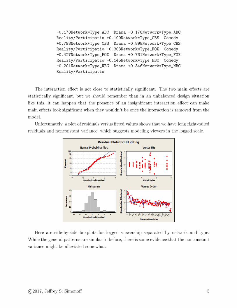
Unfortunately, a plot of residuals versus fitted values shows that we have long right-tailed
residuals and nonconstant variance, which suggests modeling viewers in the logged scale.
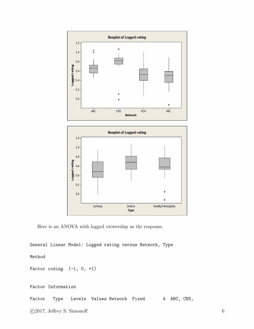
Here are side-by-side boxplots for logged viewership separated by network and type.
While the general patterns are similar to before, there is some evidence that the nonconstant
variance might be alleviated somewhat.
c©2017, Jeffrey S. Simonoff 5
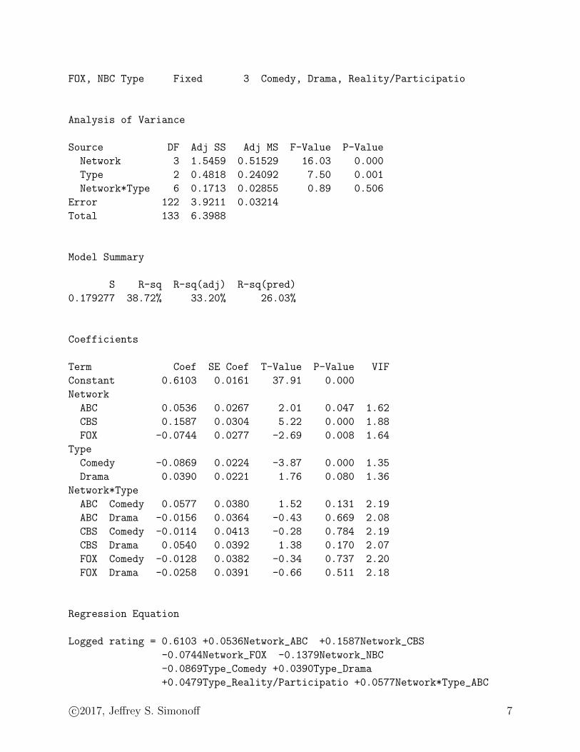
Here is an ANOVA with logged viewership as the response.
General Linear Model: Logged rating versus Network, Type
Method
Factor coding (-1, 0, +1)
Factor Information
Factor Type Levels Values Network Fixed 4 ABC, CBS,
c©2017, Jeffrey S. Simonoff 6
FOX, NBC Type Fixed 3 Comedy, Drama, Reality/Participatio
Analysis of Variance
Source DF Adj SS Adj MS F-Value P-Value
Network 3 1.5459 0.51529 16.03 0.000
Type 2 0.4818 0.24092 7.50 0.001
Network*Type 6 0.1713 0.02855 0.89 0.506
Error 122 3.9211 0.03214
Total 133 6.3988
Model Summary
S R-sq R-sq(adj) R-sq(pred)
0.179277 38.72% 33.20% 26.03%
Coefficients
Term Coef SE Coef T-Value P-Value VIF
Constant 0.6103 0.0161 37.91 0.000
Network
ABC 0.0536 0.0267 2.01 0.047 1.62
CBS 0.1587 0.0304 5.22 0.000 1.88
FOX -0.0744 0.0277 -2.69 0.008 1.64
Type
Comedy -0.0869 0.0224 -3.87 0.000 1.35
Drama 0.0390 0.0221 1.76 0.080 1.36
Network*Type
ABC Comedy 0.0577 0.0380 1.52 0.131 2.19
ABC Drama -0.0156 0.0364 -0.43 0.669 2.08
CBS Comedy -0.0114 0.0413 -0.28 0.784 2.19
CBS Drama 0.0540 0.0392 1.38 0.170 2.07
FOX Comedy -0.0128 0.0382 -0.34 0.737 2.20
FOX Drama -0.0258 0.0391 -0.66 0.511 2.18
Regression Equation
Logged rating = 0.6103 +0.0536Network_ABC +0.1587Network_CBS
-0.0744Network_FOX -0.1379Network_NBC
-0.0869Type_Comedy +0.0390Type_Drama
+0.0479Type_Reality/Participatio +0.0577Network*Type_ABC
c©2017, Jeffrey S. Simonoff 7
Comedy -0.0156Network*Type_ABC Drama
-0.0421Network*Type_ABC Reality/Participatio
-0.0114Network*Type_CBS Comedy +0.0540Network*Type_CBS
Drama -0.0427Network*Type_CBS Reality/Participatio
-0.0128Network*Type_FOX Comedy -0.0258Network*Type_FOX
Drama +0.0386Network*Type_FOX Reality/Participatio
-0.0336Network*Type_NBC Comedy -0.0126Network*Type_NBC
Drama +0.0462Network*Type_NBC Reality/Participatio
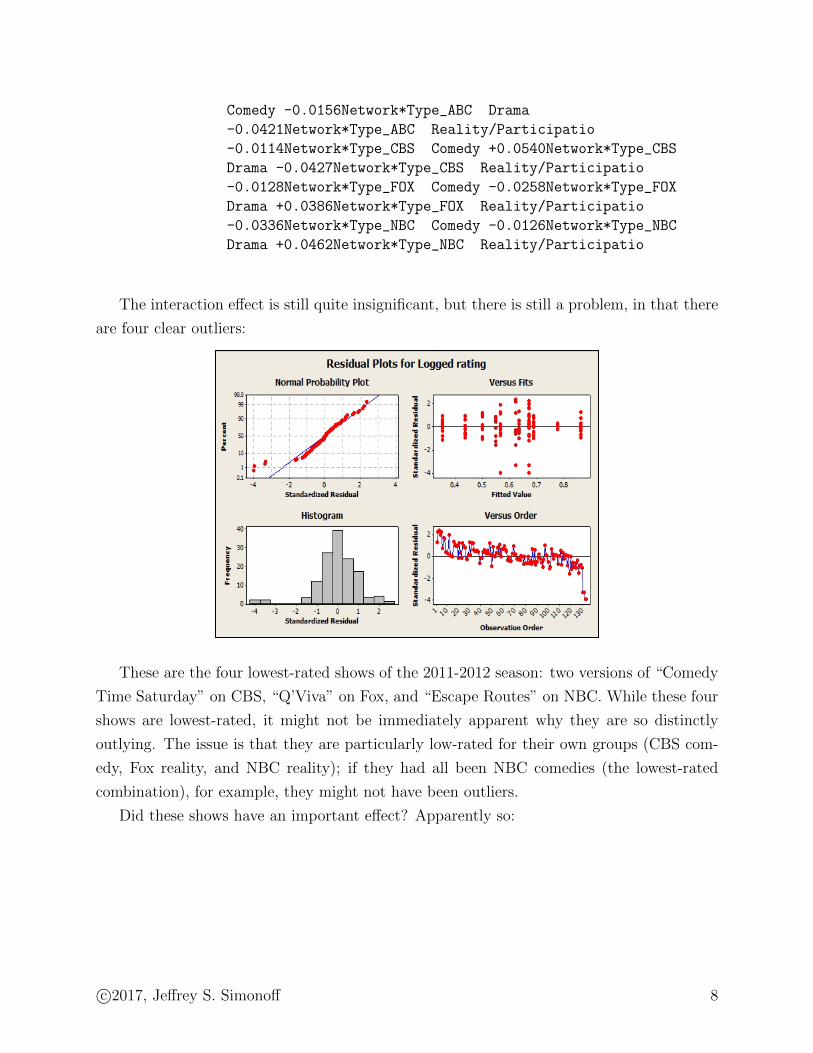
The interaction effect is still quite insignificant, but there is still a problem, in that there
are four clear outliers:
These are the four lowest-rated shows of the 2011-2012 season: two versions of “Comedy
Time Saturday” on CBS, “Q’Viva” on Fox, and “Escape Routes” on NBC. While these four
shows are lowest-rated, it might not be immediately apparent why they are so distinctly
outlying. The issue is that they are particularly low-rated for their own groups (CBS com-
edy, Fox reality, and NBC reality); if they had all been NBC comedies (the lowest-rated
combination), for example, they might not have been outliers.
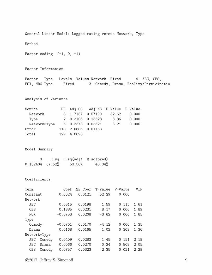
Did these shows have an important effect? Apparently so:
c©2017, Jeffrey S. Simonoff 8
General Linear Model: Logged rating versus Network, Type
Method
Factor coding (-1, 0, +1)
Factor Information
Factor Type Levels Values Network Fixed 4 ABC, CBS,
FOX, NBC Type Fixed 3 Comedy, Drama, Reality/Participatio
Analysis of Variance
Source DF Adj SS Adj MS F-Value P-Value
Network 3 1.7157 0.57190 32.62 0.000
Type 2 0.3106 0.15528 8.86 0.000
Network*Type 6 0.3373 0.05621 3.21 0.006
Error 118 2.0686 0.01753
Total 129 4.8693
Model Summary
S R-sq R-sq(adj) R-sq(pred)
0.132404 57.52% 53.56% 48.34%
Coefficients
Term Coef SE Coef T-Value P-Value VIF
Constant 0.6324 0.0121 52.29 0.000
Network
ABC 0.0315 0.0198 1.59 0.115 1.61
CBS 0.1885 0.0231 8.17 0.000 1.89
FOX -0.0753 0.0208 -3.62 0.000 1.65
Type
Comedy -0.0701 0.0170 -4.12 0.000 1.35
Drama 0.0168 0.0165 1.02 0.309 1.36
Network*Type
ABC Comedy 0.0409 0.0283 1.45 0.151 2.19
ABC Drama 0.0066 0.0270 0.24 0.808 2.05
CBS Comedy 0.0757 0.0323 2.35 0.021 2.29
c©2017, Jeffrey S. Simonoff 9
CBS Drama 0.0242 0.0294 0.82 0.412 2.10
FOX Comedy -0.0509 0.0286 -1.78 0.078 2.18
FOX Drama -0.0249 0.0292 -0.85 0.395 2.12
Regression Equation
Logged rating = 0.6324 +0.0315Network_ABC +0.1885Network_CBS
-0.0753Network_FOX -0.1447Network_NBC
-0.0701Type_Comedy +0.0168Type_Drama
+0.0532Type_Reality/Participatio +0.0409Network*Type_ABC
Comedy +0.0066Network*Type_ABC Drama
-0.0475Network*Type_ABC Reality/Participatio
+0.0757Network*Type_CBS Comedy +0.0242Network*Type_CBS
Drama -0.0999Network*Type_CBS Reality/Participatio
-0.0509Network*Type_FOX Comedy -0.0249Network*Type_FOX
Drama +0.0758Network*Type_FOX Reality/Participatio
-0.0657Network*Type_NBC Comedy -0.0059Network*Type_NBC
Drama +0.0716Network*Type_NBC Reality/Participatio
Means
Fitted
Term Mean SE Mean
Network
ABC 0.6639 0.0222
CBS 0.8209 0.0278
FOX 0.5571 0.0239
NBC 0.4877 0.0224
Type
Comedy 0.5624 0.0207
Drama 0.6493 0.0194
Reality/Participatio 0.6857 0.0227
Network*Type
ABC Comedy 0.6348 0.0399
ABC Drama 0.6873 0.0354
ABC Reality/Participatio 0.6697 0.0399
CBS Comedy 0.8266 0.0468
CBS Drama 0.8620 0.0354
CBS Reality/Participatio 0.7742 0.0592
FOX Comedy 0.4362 0.0382
FOX Drama 0.5491 0.0419
FOX Reality/Participatio 0.6861 0.0441
NBC Comedy 0.3519 0.0399
NBC Drama 0.4987 0.0419
c©2017, Jeffrey S. Simonoff 10
NBC Reality/Participatio 0.6126 0.0342
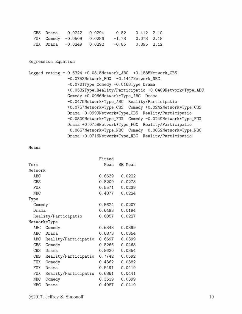
The interaction effect is now statistically significant, so apparently the relative perfor-
mance of comedies, dramas, and reality shows differs from network to network. Note that in
a model that includes the interaction effect the fitted (and predicted) values correspond to
the means for each network / type combination, which is the average response value for each
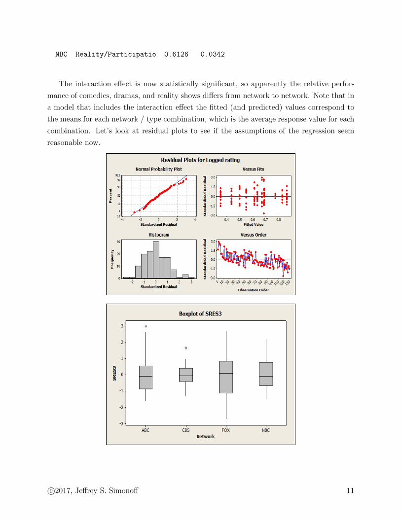
combination. Let’s look at residual plots to see if the assumptions of the regression seem
reasonable now.
c©2017, Jeffrey S. Simonoff 11
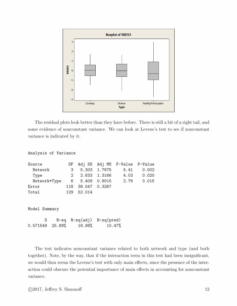
The residual plots look better than they have before. There is still a bit of a right tail, and
some evidence of nonconstant variance. We can look at Levene’s test to see if nonconstant
variance is indicated by it.
Analysis of Variance
Source DF Adj SS Adj MS F-Value P-Value
Network 3 5.303 1.7675 5.41 0.002
Type 2 2.633 1.3166 4.03 0.020
Network*Type 6 5.409 0.9015 2.76 0.015
Error 118 38.547 0.3267
Total 129 52.014
Model Summary
S R-sq R-sq(adj) R-sq(pred)
0.571549 25.89% 18.98% 10.47%
The test indicates nonconstant variance related to both network and type (and both
together). Note, by the way, that if the interaction term in this test had been insignificant,
we would then rerun the Levene’s test with only main effects, since the presence of the inter-
action could obscure the potential importance of main effects in accounting for nonconstant
variance.
c©2017, Jeffrey S. Simonoff 12
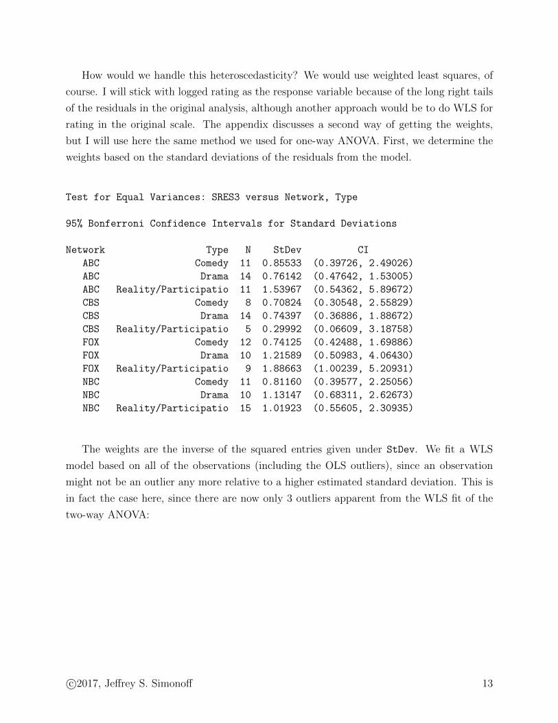
How would we handle this heteroscedasticity? We would use weighted least squares, of
course. I will stick with logged rating as the response variable because of the long right tails
of the residuals in the original analysis, although another approach would be to do WLS for
rating in the original scale. The appendix discusses a second way of getting the weights,
but I will use here the same method we used for one-way ANOVA. First, we determine the
weights based on the standard deviations of the residuals from the model.
Test for Equal Variances: SRES3 versus Network, Type
95% Bonferroni Confidence Intervals for Standard Deviations
Network Type N StDev CI
ABC Comedy 11 0.85533 (0.39726, 2.49026)
ABC Drama 14 0.76142 (0.47642, 1.53005)
ABC Reality/Participatio 11 1.53967 (0.54362, 5.89672)
CBS Comedy 8 0.70824 (0.30548, 2.55829)
CBS Drama 14 0.74397 (0.36886, 1.88672)
CBS Reality/Participatio 5 0.29992 (0.06609, 3.18758)
FOX Comedy 12 0.74125 (0.42488, 1.69886)
FOX Drama 10 1.21589 (0.50983, 4.06430)
FOX Reality/Participatio 9 1.88663 (1.00239, 5.20931)
NBC Comedy 11 0.81160 (0.39577, 2.25056)
NBC Drama 10 1.13147 (0.68311, 2.62673)
NBC Reality/Participatio 15 1.01923 (0.55605, 2.30935)
The weights are the inverse of the squared entries given under StDev. We fit a WLS
model based on all of the observations (including the OLS outliers), since an observation
might not be an outlier any more relative to a higher estimated standard deviation. This is
in fact the case here, since there are now only 3 outliers apparent from the WLS fit of the
two-way ANOVA:
c©2017, Jeffrey S. Simonoff 13
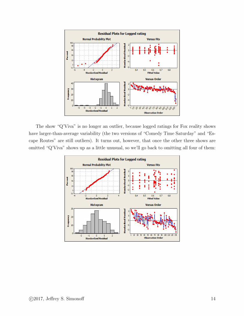
The show “Q’Viva” is no longer an outlier, because logged ratings for Fox reality shows
have larger-than-average variability (the two versions of “Comedy Time Saturday” and “Es-
cape Routes” are still outliers). It turns out, however, that once the other three shows are
omitted “Q’Viva” shows up as a little unusual, so we’ll go back to omitting all four of them:
c©2017, Jeffrey S. Simonoff 14
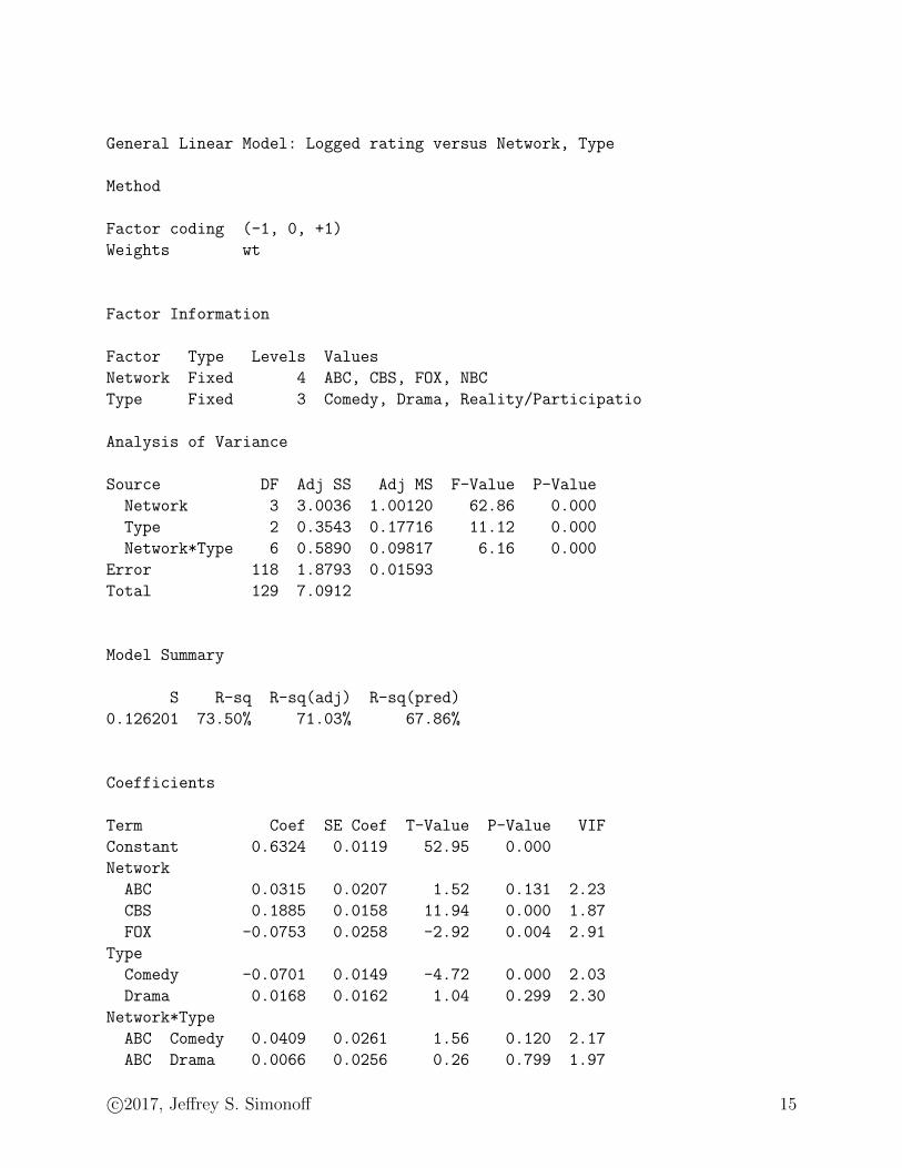
General Linear Model: Logged rating versus Network, Type
Method
Factor coding (-1, 0, +1)
Weights wt
Factor Information
Factor Type Levels Values
Network Fixed 4 ABC, CBS, FOX, NBC
Type Fixed 3 Comedy, Drama, Reality/Participatio
Analysis of Variance
Source DF Adj SS Adj MS F-Value P-Value
Network 3 3.0036 1.00120 62.86 0.000
Type 2 0.3543 0.17716 11.12 0.000
Network*Type 6 0.5890 0.09817 6.16 0.000
Error 118 1.8793 0.01593
Total 129 7.0912
Model Summary
S R-sq R-sq(adj) R-sq(pred)
0.126201 73.50% 71.03% 67.86%
Coefficients
Term Coef SE Coef T-Value P-Value VIF
Constant 0.6324 0.0119 52.95 0.000
Network
ABC 0.0315 0.0207 1.52 0.131 2.23
CBS 0.1885 0.0158 11.94 0.000 1.87
FOX -0.0753 0.0258 -2.92 0.004 2.91
Type
Comedy -0.0701 0.0149 -4.72 0.000 2.03
Drama 0.0168 0.0162 1.04 0.299 2.30
Network*Type
ABC Comedy 0.0409 0.0261 1.56 0.120 2.17
ABC Drama 0.0066 0.0256 0.26 0.799 1.97
c©2017, Jeffrey S. Simonoff 15
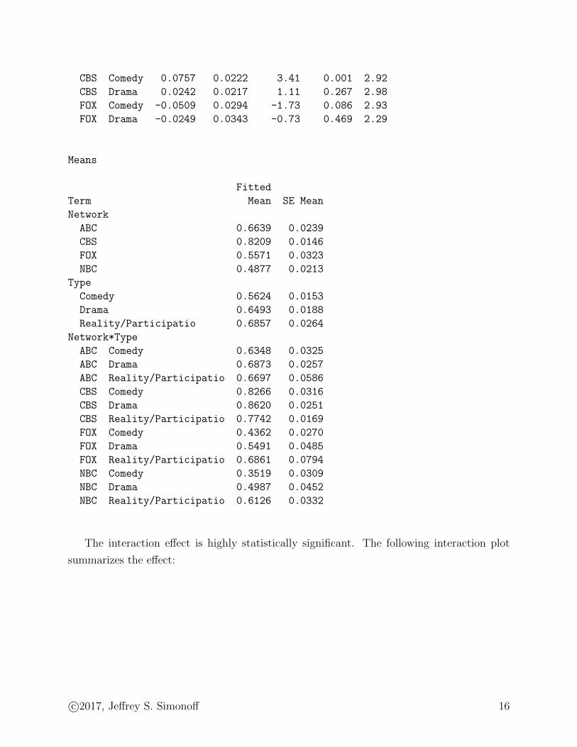
CBS Comedy 0.0757 0.0222 3.41 0.001 2.92
CBS Drama 0.0242 0.0217 1.11 0.267 2.98
FOX Comedy -0.0509 0.0294 -1.73 0.086 2.93
FOX Drama -0.0249 0.0343 -0.73 0.469 2.29
Means
Fitted
Term Mean SE Mean
Network
ABC 0.6639 0.0239
CBS 0.8209 0.0146
FOX 0.5571 0.0323
NBC 0.4877 0.0213
Type
Comedy 0.5624 0.0153
Drama 0.6493 0.0188
Reality/Participatio 0.6857 0.0264
Network*Type
ABC Comedy 0.6348 0.0325
ABC Drama 0.6873 0.0257
ABC Reality/Participatio 0.6697 0.0586
CBS Comedy 0.8266 0.0316
CBS Drama 0.8620 0.0251
CBS Reality/Participatio 0.7742 0.0169
FOX Comedy 0.4362 0.0270
FOX Drama 0.5491 0.0485
FOX Reality/Participatio 0.6861 0.0794
NBC Comedy 0.3519 0.0309
NBC Drama 0.4987 0.0452
NBC Reality/Participatio 0.6126 0.0332
The interaction effect is highly statistically significant. The following interaction plot
summarizes the effect:
c©2017, Jeffrey S. Simonoff 16
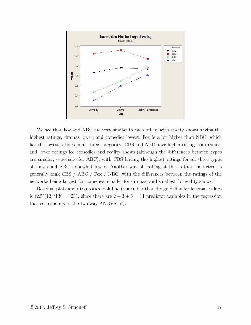
We see that Fox and NBC are very similar to each other, with reality shows having the
highest ratings, dramas lower, and comedies lowest; Fox is a bit higher than NBC, which
has the lowest ratings in all three categories. CBS and ABC have higher ratings for dramas,
and lower ratings for comedies and reality shows (although the differences between types
are smaller, especially for ABC), with CBS having the highest ratings for all three types
of shows and ABC somewhat lower. Another way of looking at this is that the networks
generally rank CBS / ABC / Fox / NBC, with the differences between the ratings of the
networks being largest for comedies, smaller for dramas, and smallest for reality shows.
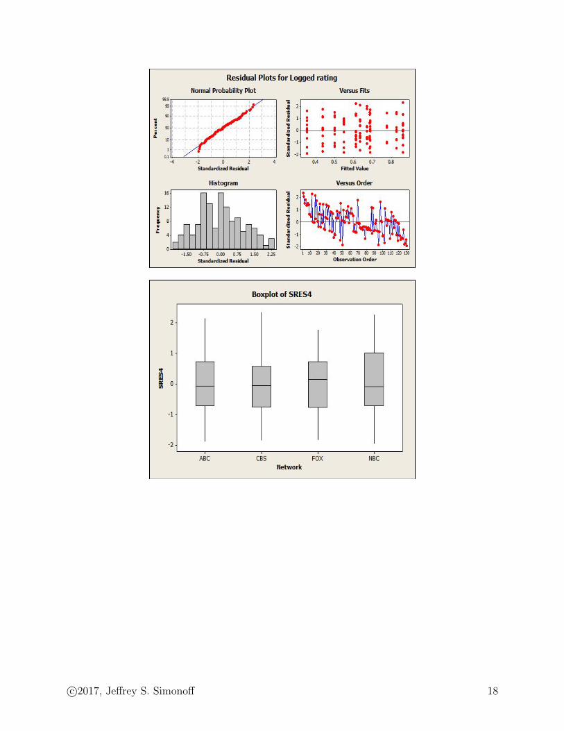
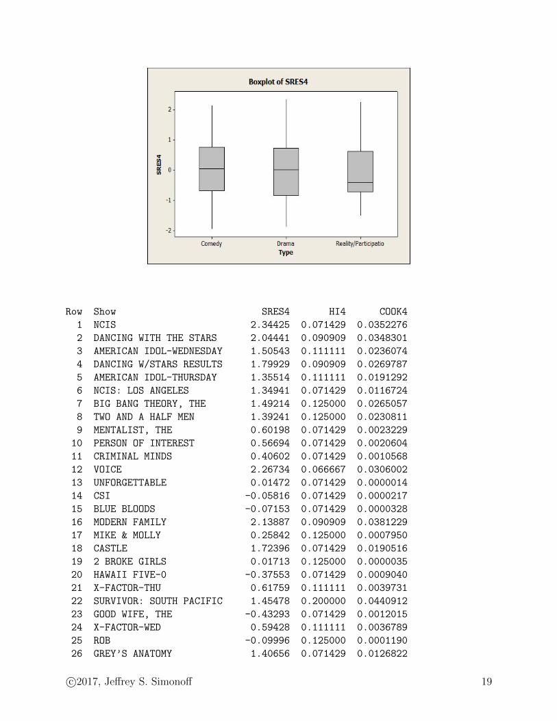
Residual plots and diagnostics look fine (remember that the guideline for leverage values
is (2.5)(12)/130 = .231, since there are 2 + 3 + 6 = 11 predictor variables in the regression
that corresponds to the two-way ANOVA fit).
c©2017, Jeffrey S. Simonoff 17
c©2017, Jeffrey S. Simonoff 18
Row Show SRES4 HI4 COOK4
1 NCIS 2.34425 0.071429 0.0352276
2 DANCING WITH THE STARS 2.04441 0.090909 0.0348301
3 AMERICAN IDOL-WEDNESDAY 1.50543 0.111111 0.0236074
4 DANCING W/STARS RESULTS 1.79929 0.090909 0.0269787
5 AMERICAN IDOL-THURSDAY 1.35514 0.111111 0.0191292
6 NCIS: LOS ANGELES 1.34941 0.071429 0.0116724
7 BIG BANG THEORY, THE 1.49214 0.125000 0.0265057
8 TWO AND A HALF MEN 1.39241 0.125000 0.0230811
9 MENTALIST, THE 0.60198 0.071429 0.0023229
10 PERSON OF INTEREST 0.56694 0.071429 0.0020604
11 CRIMINAL MINDS 0.40602 0.071429 0.0010568
12 VOICE 2.26734 0.066667 0.0306002
13 UNFORGETTABLE 0.01472 0.071429 0.0000014
14 CSI -0.05816 0.071429 0.0000217
15 BLUE BLOODS -0.07153 0.071429 0.0000328
16 MODERN FAMILY 2.13887 0.090909 0.0381229
17 MIKE & MOLLY 0.25842 0.125000 0.0007950
18 CASTLE 1.72396 0.071429 0.0190516
19 2 BROKE GIRLS 0.01713 0.125000 0.0000035
20 HAWAII FIVE-0 -0.37553 0.071429 0.0009040
21 X-FACTOR-THU 0.61759 0.111111 0.0039731
22 SURVIVOR: SOUTH PACIFIC 1.45478 0.200000 0.0440912
23 GOOD WIFE, THE -0.43293 0.071429 0.0012015
24 X-FACTOR-WED 0.59428 0.111111 0.0036789
25 ROB -0.09996 0.125000 0.0001190
26 GREY’S ANATOMY 1.40656 0.071429 0.0126822
c©2017, Jeffrey S. Simonoff 19
27 CSI: MIAMI -0.57951 0.071429 0.0021528
28 CSI: NY -0.63942 0.071429 0.0026209
29 AMAZING RACE 19 0.37004 0.200000 0.0028527
30 AMERICA’S GOT TALENT-TUE 1.37307 0.066667 0.0112222
31 SURVIVOR: ONE WORLD 0.22247 0.200000 0.0010311
32 AMERICA’S GOT TALENT-MON 1.27379 0.066667 0.0096581
33 VOICE:RESULTS SHOW 1.23807 0.066667 0.0091239
34 HOW I MET YOUR MOTHER -0.74643 0.125000 0.0066328
35 BODY OF PROOF 0.81381 0.071429 0.0042454
36 ONCE UPON A TIME 0.78129 0.071429 0.0039130
37 RULES OF ENGAGEMENT -0.81845 0.125000 0.0079745
38 DESPERATE HOUSEWIVES 0.65732 0.071429 0.0027697
39 GIFTED MAN, A -1.26643 0.071429 0.0102810
40 UNDERCOVER BOSS -0.97691 0.200000 0.0198823
41 AMAZING RACE 20 -1.07038 0.200000 0.0238689
42 BACHELOR, THE 0.33848 0.090909 0.0009548
43 LAST MAN STANDING 0.88545 0.090909 0.0065335
44 BACHELORETTE, THE 0.29467 0.090909 0.0007236
45 REVENGE 0.33672 0.071429 0.0007268
46 MIDDLE, THE 0.74841 0.090909 0.0046676
47 HOW TO BE A GENTLEMAN -1.49526 0.125000 0.0266167
48 HARRY’S LAW 1.49744 0.100000 0.0207624
49 MISSING 0.09756 0.071429 0.0000610
50 NYC 22 -1.85980 0.071429 0.0221721
51 BONES 0.97554 0.100000 0.0088118
52 SCANDAL 0.01185 0.071429 0.0000009
53 PRIVATE PRACTICE -0.06568 0.071429 0.0000277
54 LAST MAN STANDING-8:30PM 0.41611 0.090909 0.0014429
55 TOUCH 0.86411 0.100000 0.0069138
56 SUBURGATORY 0.36258 0.090909 0.0010955
57 LAW AND ORDER:SVU 1.25936 0.100000 0.0146852
58 DUETS -0.08371 0.090909 0.0000584
59 GLEE 0.72202 0.100000 0.0048270
60 TERRA NOVA 0.71540 0.100000 0.0047388
61 SMASH 1.09745 0.100000 0.0111518
62 HOUSE 0.64156 0.100000 0.0038112
63 ALCATRAZ 0.50957 0.100000 0.0024042
64 CHARLIE’S ANGELS -0.79356 0.071429 0.0040368
65 MAN UP! -0.23437 0.090909 0.0004577
66 GCB -0.85097 0.071429 0.0046420
67 ROOKIE BLUE -0.86254 0.071429 0.0047691
68 BIGGEST LOSER 13 -0.05840 0.066667 0.0000203
69 NEW GIRL 1.76605 0.083333 0.0236283
70 APPRENTICE 12 -0.14622 0.066667 0.0001273
71 BIGGEST LOSER 12 -0.14622 0.066667 0.0001273
c©2017, Jeffrey S. Simonoff 20
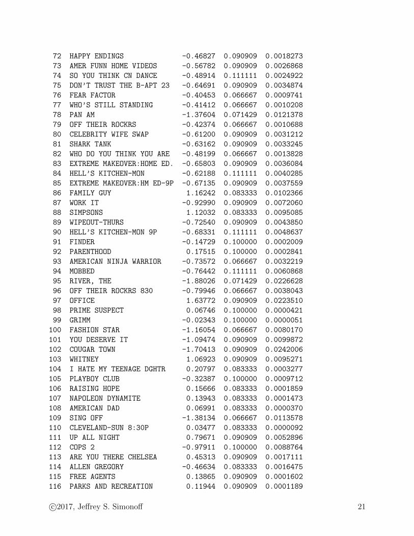
72 HAPPY ENDINGS -0.46827 0.090909 0.0018273
73 AMER FUNN HOME VIDEOS -0.56782 0.090909 0.0026868
74 SO YOU THINK CN DANCE -0.48914 0.111111 0.0024922
75 DON’T TRUST THE B-APT 23 -0.64691 0.090909 0.0034874
76 FEAR FACTOR -0.40453 0.066667 0.0009741
77 WHO’S STILL STANDING -0.41412 0.066667 0.0010208
78 PAN AM -1.37604 0.071429 0.0121378
79 OFF THEIR ROCKRS -0.42374 0.066667 0.0010688
80 CELEBRITY WIFE SWAP -0.61200 0.090909 0.0031212
81 SHARK TANK -0.63162 0.090909 0.0033245
82 WHO DO YOU THINK YOU ARE -0.48199 0.066667 0.0013828
83 EXTREME MAKEOVER:HOME ED. -0.65803 0.090909 0.0036084
84 HELL’S KITCHEN-MON -0.62188 0.111111 0.0040285
85 EXTREME MAKEOVER:HM ED-9P -0.67135 0.090909 0.0037559
86 FAMILY GUY 1.16242 0.083333 0.0102366
87 WORK IT -0.92990 0.090909 0.0072060
88 SIMPSONS 1.12032 0.083333 0.0095085
89 WIPEOUT-THURS -0.72540 0.090909 0.0043850
90 HELL’S KITCHEN-MON 9P -0.68331 0.111111 0.0048637
91 FINDER -0.14729 0.100000 0.0002009
92 PARENTHOOD 0.17515 0.100000 0.0002841
93 AMERICAN NINJA WARRIOR -0.73572 0.066667 0.0032219
94 MOBBED -0.76442 0.111111 0.0060868
95 RIVER, THE -1.88026 0.071429 0.0226628
96 OFF THEIR ROCKRS 830 -0.79946 0.066667 0.0038043
97 OFFICE 1.63772 0.090909 0.0223510
98 PRIME SUSPECT 0.06746 0.100000 0.0000421
99 GRIMM -0.02343 0.100000 0.0000051
100 FASHION STAR -1.16054 0.066667 0.0080170
101 YOU DESERVE IT -1.09474 0.090909 0.0099872
102 COUGAR TOWN -1.70413 0.090909 0.0242006
103 WHITNEY 1.06923 0.090909 0.0095271
104 I HATE MY TEENAGE DGHTR 0.20797 0.083333 0.0003277
105 PLAYBOY CLUB -0.32387 0.100000 0.0009712
106 RAISING HOPE 0.15666 0.083333 0.0001859
107 NAPOLEON DYNAMITE 0.13943 0.083333 0.0001473
108 AMERICAN DAD 0.06991 0.083333 0.0000370
109 SING OFF -1.38134 0.066667 0.0113578
110 CLEVELAND-SUN 8:30P 0.03477 0.083333 0.0000092
111 UP ALL NIGHT 0.79671 0.090909 0.0052896
112 COPS 2 -0.97911 0.100000 0.0088764
113 ARE YOU THERE CHELSEA 0.45313 0.090909 0.0017111
114 ALLEN GREGORY -0.46634 0.083333 0.0016475
115 FREE AGENTS 0.13865 0.090909 0.0001602
116 PARKS AND RECREATION 0.11944 0.090909 0.0001189
c©2017, Jeffrey S. Simonoff 21
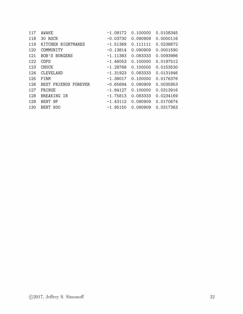
117 AWAKE -1.08172 0.100000 0.0108345
118 30 ROCK -0.03730 0.090909 0.0000116
119 KITCHEN NIGHTMARES -1.51369 0.111111 0.0238672
120 COMMUNITY -0.13814 0.090909 0.0001590
121 BOB’S BURGERS -1.11383 0.083333 0.0093986
122 COPS -1.46053 0.100000 0.0197512
123 CHUCK -1.28768 0.100000 0.0153530
124 CLEVELAND -1.31923 0.083333 0.0131846
125 FIRM -1.38017 0.100000 0.0176376
126 BEST FRIENDS FOREVER -0.65684 0.090909 0.0035953
127 FRINGE -1.84127 0.100000 0.0313916
128 BREAKING IN -1.75813 0.083333 0.0234169
129 BENT 9P -1.43112 0.090909 0.0170674
130 BENT 930 -1.95150 0.090909 0.0317363
c©2017, Jeffrey S. Simonoff 22
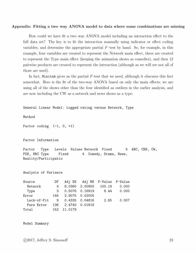
Appendix: Fitting a two–way ANOVA model to data where some combinations are missing
How could we have fit a two–way ANOVA model including an interaction effect to the
full data set? The key is to fit the interaction manually using indicator or effect coding
variables, and determine the appropriate partial F–test by hand. So, for example, in this
example, four variables are created to represent the Network main effect, three are created
to represent the Type main effect (keeping the animation shows as comedies), and then 12
pairwise products are created to represent the interaction (although as we will see not all of
those are used).
In fact, Minitab gives us the partial F -test that we need, although it obscures this fact
somewhat. Here is the fit of the two-way ANOVA based on only the main effects; we are
using all of the shows other than the four identified as outliers in the earlier analysis, and
are now including the CW as a network and news shows as a type:
General Linear Model: Logged rating versus Network, Type
Method
Factor coding (-1, 0, +1)
Factor Information
Factor Type Levels Values Network Fixed 5 ABC, CBS, CW,
FOX, NBC Type Fixed 4 Comedy, Drama, News,
Reality/Participatio
Analysis of Variance
Source DF Adj SS Adj MS F-Value P-Value
Network 4 8.0360 2.00900 100.19 0.000
Type 3 0.5076 0.16919 8.44 0.000
Error 145 2.9075 0.02005
Lack-of-Fit 9 0.4335 0.04816 2.65 0.007
Pure Error 136 2.4740 0.01819
Total 152 11.0179
Model Summary
c©2017, Jeffrey S. Simonoff 23
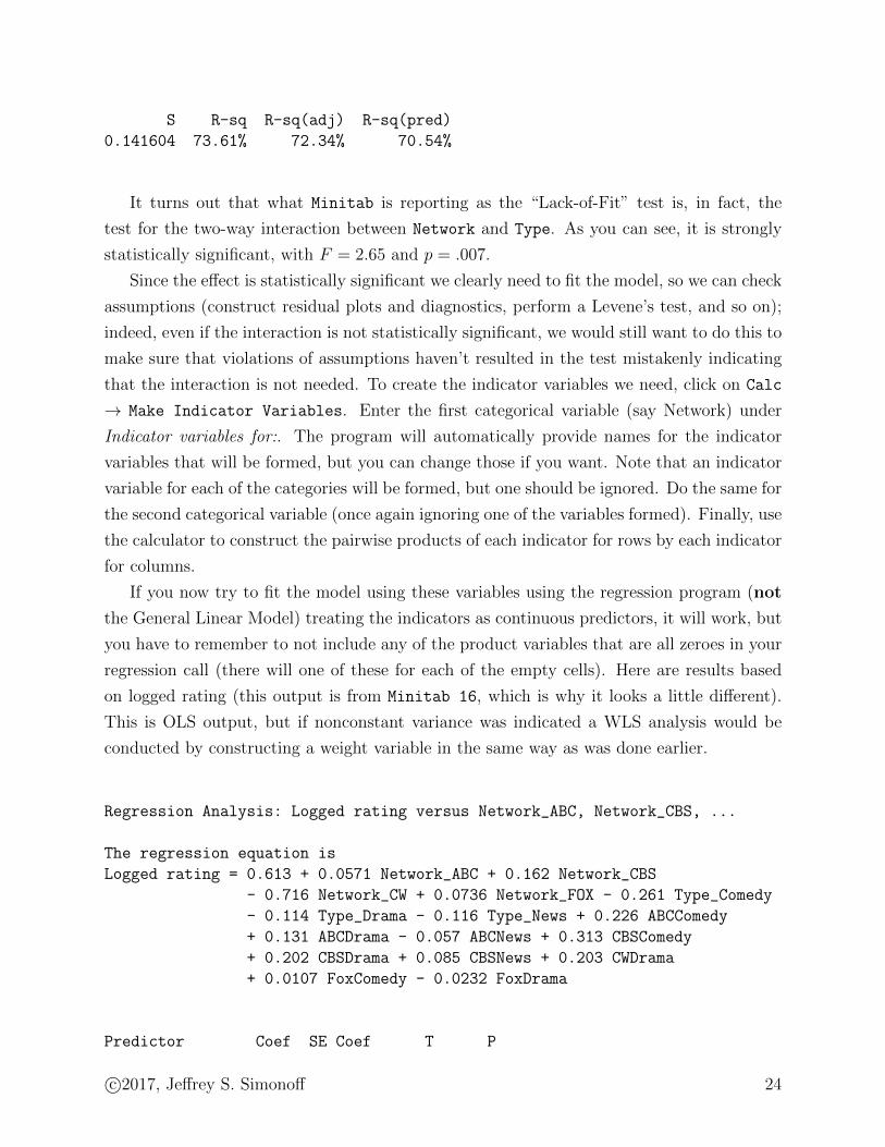
S R-sq R-sq(adj) R-sq(pred)
0.141604 73.61% 72.34% 70.54%
It turns out that what Minitab is reporting as the “Lack-of-Fit” test is, in fact, the
test for the two-way interaction between Network and Type. As you can see, it is strongly
statistically significant, with F = 2.65 and p = .007.
Since the effect is statistically significant we clearly need to fit the model, so we can check
assumptions (construct residual plots and diagnostics, perform a Levene’s test, and so on);
indeed, even if the interaction is not statistically significant, we would still want to do this to
make sure that violations of assumptions haven’t resulted in the test mistakenly indicating
that the interaction is not needed. To create the indicator variables we need, click on Calc
→ Make Indicator Variables. Enter the first categorical variable (say Network) under
Indicator variables for:. The program will automatically provide names for the indicator
variables that will be formed, but you can change those if you want. Note that an indicator
variable for each of the categories will be formed, but one should be ignored. Do the same for
the second categorical variable (once again ignoring one of the variables formed). Finally, use
the calculator to construct the pairwise products of each indicator for rows by each indicator
for columns.
If you now try to fit the model using these variables using the regression program (not
the General Linear Model) treating the indicators as continuous predictors, it will work, but
you have to remember to not include any of the product variables that are all zeroes in your
regression call (there will one of these for each of the empty cells). Here are results based
on logged rating (this output is from Minitab 16, which is why it looks a little different).
This is OLS output, but if nonconstant variance was indicated a WLS analysis would be
conducted by constructing a weight variable in the same way as was done earlier.
Regression Analysis: Logged rating versus Network_ABC, Network_CBS, ...
The regression equation is
Logged rating = 0.613 + 0.0571 Network_ABC + 0.162 Network_CBS
- 0.716 Network_CW + 0.0736 Network_FOX - 0.261 Type_Comedy
- 0.114 Type_Drama - 0.116 Type_News + 0.226 ABCComedy
+ 0.131 ABCDrama - 0.057 ABCNews + 0.313 CBSComedy
+ 0.202 CBSDrama + 0.085 CBSNews + 0.203 CWDrama
+ 0.0107 FoxComedy - 0.0232 FoxDrama
Predictor Coef SE Coef T P
c©2017, Jeffrey S. Simonoff 24
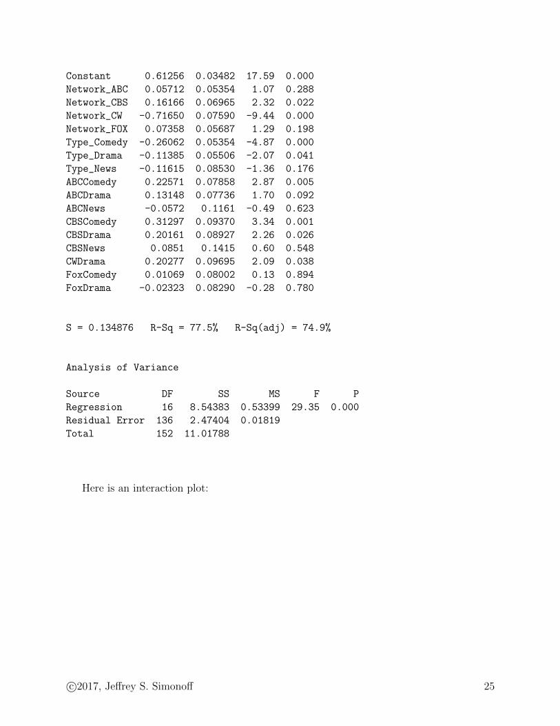
Constant 0.61256 0.03482 17.59 0.000
Network_ABC 0.05712 0.05354 1.07 0.288
Network_CBS 0.16166 0.06965 2.32 0.022
Network_CW -0.71650 0.07590 -9.44 0.000
Network_FOX 0.07358 0.05687 1.29 0.198
Type_Comedy -0.26062 0.05354 -4.87 0.000
Type_Drama -0.11385 0.05506 -2.07 0.041
Type_News -0.11615 0.08530 -1.36 0.176
ABCComedy 0.22571 0.07858 2.87 0.005
ABCDrama 0.13148 0.07736 1.70 0.092
ABCNews -0.0572 0.1161 -0.49 0.623
CBSComedy 0.31297 0.09370 3.34 0.001
CBSDrama 0.20161 0.08927 2.26 0.026
CBSNews 0.0851 0.1415 0.60 0.548
CWDrama 0.20277 0.09695 2.09 0.038
FoxComedy 0.01069 0.08002 0.13 0.894
FoxDrama -0.02323 0.08290 -0.28 0.780
S = 0.134876 R-Sq = 77.5% R-Sq(adj) = 74.9%
Analysis of Variance
Source DF SS MS F P
Regression 16 8.54383 0.53399 29.35 0.000
Residual Error 136 2.47404 0.01819
Total 152 11.01788
Here is an interaction plot:
c©2017, Jeffrey S. Simonoff 25
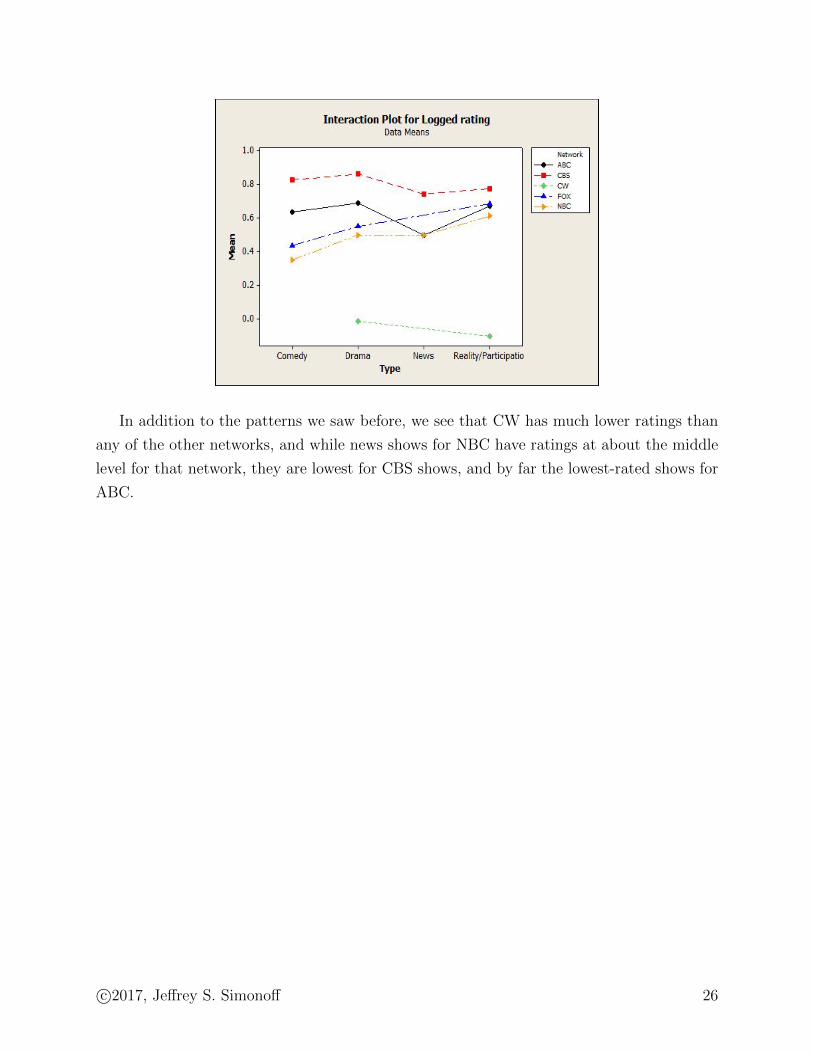
In addition to the patterns we saw before, we see that CW has much lower ratings than
any of the other networks, and while news shows for NBC have ratings at about the middle
level for that network, they are lowest for CBS shows, and by far the lowest-rated shows for
ABC.
c©2017, Jeffrey S. Simonoff 26
Minitab commands
Two–way analysis of variance is conducted by clicking on Stat → ANOVA → General
Linear Model→ Fit General Linear Model. Enter the target variable under Responses:
and the two categorizing predicting variables under Factors:. To include the interaction
effect, click on Model. Highlight the two factor variables to the left, and click on Add.
This will add the variables “multiplied” by each other (i.e., ROW*COL) under Terms in the
model:. Residual plots and storage are obtained as stated earlier. To get effect estimates for
your model, click on Options and then All terms in the model in the drop-down menu
next to Means:. Note that the effects for main effects are not interpretable in the presence
of the interaction.
To construct an interaction plot, click on Stat→ ANOVA→ Interaction plot. Enter the
two predicting variables that define the interaction under Factors:, and enter the response
variable next to the box labeled Responses:.
Levene’s test is constructed in the usual way by fitting a two-way ANOVA with the
absolute standardized residuals as the response. Note that if nij = 1 in some cell(s) the
standardized residual produced by Minitab for that single observation will be set to the
missing value code * because technically the standardized residual is undefined (hii = 1
for the observation in a cell with nij = 1, so the standardized residual is 0/0). For such
an observation set the standardized residual equal to 0 and the weight equal to 1, since
the observation will be fit perfectly (resulting in a zero residual) no matter what weight is
used. Remember that if the interaction effect is not significant in the Levene’s test ANOVA
you should run it again with the interaction effect removed to see if it is related to one
or the other main effect; to do so highlight the product term in the box under Terms in
the model and click “X”. If weights for a weighted least squares fit depend on only one
of the effects, they can be determined using the method described for one-way ANOVA
models. If weights are needed based on two categorical variables (either if the interaction
effect in the Levene’s test is statistically significant or if it is not but both main effects in the
Levene’s test are), they can be estimated simultaneously. Click on Stat → ANOVA → Test
for Equal Variances. Enter the residuals from the OLS fit under Response:, and the two
variables under Factors:. The resultant output gives the standard deviations of the residuals
separated by the levels of the variables under “StDev” in the portion labeled Bonferroni
confidence intervals for standard deviations. The weights are one over the squared
standard deviations. Note that you should not use the tests provided in the output as
your test of constant variance in a two-way ANOVA, as they do not take into account the
potential structure in the nonconstant variance; construct Levene’s test as is described in
the handout. An alternative approach to get weights is to estimate the variances in the way
c©2017, Jeffrey S. Simonoff 27
that is discussed for a numerical predictor in the Appendix of the CAPM handout. That is,
save the standardized residuals SRES from the original two–way ANOVA, perform a two-way
ANOVA with log(SRES ∗ SRES) as the target variable, saving the fitted values; and then set
the weights equal to WT = 1/exp(FITS).
To construct a table tabulating counts of the observations separated by a cross-classification
of predictive variables, click Stat → Tables → Cross Tabulation and Chi-Square. En-
ter the variables that define the effects in the ANOVA under Categorical variables (one
under For rows and the other under For columns). To get a table of means of the re-
sponse variable separated by the predicting variables, click Stat→ Tables→ Descriptive
Statistics. Enter the variables that define the effects in the ANOVA under Categorical
variables (one under For rows and the other under For columns), and click on Associated
Variables. Enter the target variable for the ANOVA under Associated variables: and
click in the box next to Means. In this situation, you might also want to obtain the esti-
mated target variable for each combination of the two predictors. This is not the response
cell mean, since the interaction effect hasn’t been fit. Using a calculator, calculate the overall
average of the fitted means given for one of the two effects (it doesn’t matter which one).
The estimated expected response for the (i, j)th combination is the ith row effect + the jth
column effect − the overall average.
If a two-way ANOVA model is fit without an interaction term, multiple comparisons for
either main effect (or both) can be obtained by highlighting and entering each term (or both)
under Choose terms for comparisons as is done for one-way ANOVA models. In a model
that includes an interaction, comparisons can be made between the different combinations
of row and column level by entering the interaction (ROW*COL for the data analyzed in this
handout) under “Terms:”.
c©2017, Jeffrey S. Simonoff 28