1

UN

U-I

NR

A W

OR

KIN

G P

AP

ER

NO

. 1

8

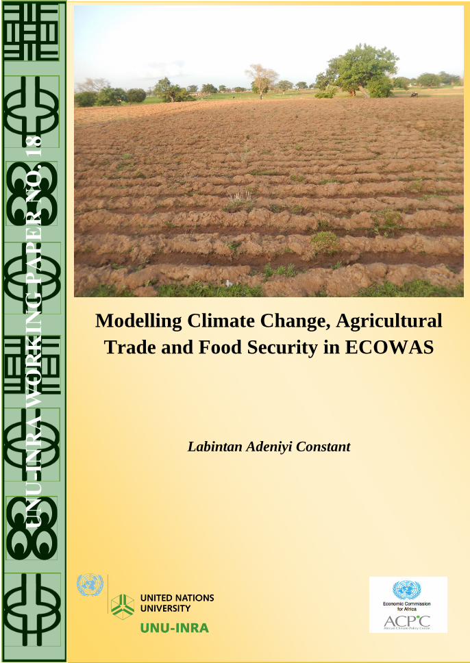
Modelling Climate Change, Agricultural

Trade and Food Security in ECOWAS

Labintan Adeniyi Constant

ii

Modelling Climate Change, Agricultural Trade and

Food Security in ECOWAS

By:

Labintan Adeniyi Constant

This work was carried out with the aid of a grant from the African Climate Policy

Centre (ACPC) of the United Nations Economic Commission for Africa

(UNECA).

iii

About UNU-INRA

The United Nations University Institute for Natural Resources in Africa (UNU-INRA) is the

second Research and Training Centre / Programme established by the UN University. The

mandate of the Institute is to promote the sustainable management of Africa’s natural

resources through research, capacity development, policy advice, knowledge sharing and

transfer. The Institute is headquartered in Accra, Ghana, and also has five Operating Units

(OUs) in Cameroon, Ivory Coast, Namibia, Senegal and Zambia.

This working paper is an output of UNU-INRA’s project entitled “Climate Change,

Agricultural Trade and Food Security in ECOWAS”, funded by the African Climate Policy

Centre (ACPC) of the United Nations Economic Commission for Africa (UNECA).

About the Author

Dr Labintan Adeniyi Constant is a Climate Change Policy Analyst at Centre de Partenariat et

d’Expertise pour le Developpement Durable (CePED), Cotonou, Benin. He produced this

paper as a Consultant of the project.

Author’s Contact

Email: donconstant@yahoo.fr

UNU-INRA Contact United Nations University Institute for Natural Resources in Africa (UNU-INRA)

2nd Floor, International House, University of Ghana Campus, Accra, Ghana

Private Mail Bag, KIA, Accra, Ghana. Tel: +233 302 213 850 Ext. 6318.

Email: inra@unu.edu Website: www.inra.unu.edu

Facebook, Twitter, and LinkedIn

© UNU-INRA, 2016

ISBN: 9789988633165

Cover Design: Praise Nutakor, UNU-INRA

Photo: UNU-INRA

Published by: UNU-INRA, Accra, Ghana

Disclaimer

The views and opinions expressed in this publication are that of the author and do not

necessarily reflect the official policy or position of the United Nations University Institute for

Natural Resources in Africa (UNU-INRA).

iv

Acknowledgments

In the implementation and eventual completion of this modelling framework, I

owe a debt of gratitude to a number of institutions and persons whose

contributions assisted us in bringing this modelling research to fruition.

First, I owe a profound gratitude to the United Nations University Institute for

Natural Resources in Africa (UNU-INRA) and the African Climate Policy

Centre (ACPC) of the United Nations Economic Commission for Africa

(UNECA), for sponsoring the modelling study.

Second, I am immensely grateful to Dr. Elias T. Ayuk, Dr. Calvin Atewamba

and Dr. Euphrasie Kouame who provided all the technical leads and input

where and when necessary during the course of the assignment.

Third, I am grateful to stakeholders in Africa and around the World, who

despite their much-tight schedules, participated in the methodology and review

workshop organized to validate this modelling framework for studying climate

change, agricultural trade and food security in ECOWAS.

v

Preface

The following is the documentation on the IAM exercise to assess the spatial

impact of climate change on agricultural production, trade flows and food

security in the ECOWAS region. The report contains model structure, model

input, output and linkage between different models. It aims to help users on

how to use the model and compute results for Analysis.

vi

Contents

Acknowledgments ...................................................................................... iv

Preface ......................................................................................................... v

List of Figures ............................................................................................ ix

List of Tables .............................................................................................. xi

General Introduction .................................................................................... 1

ECOLAND - Land Allocation Model .......................................................... 4

Introduction .......................................................................................... 4

Model Overviews .................................................................................. 5

Description ........................................................................................ 5

Model Data ........................................................................................ 6

Model Results .................................................................................. 12

Model Calibration ........................................................................... 13

Model Structure .................................................................................. 15

Notations ......................................................................................... 15

Parameters ...................................................................................... 15

Variables .......................................................................................... 17

Equations ........................................................................................ 18

Model Integration ............................................................................... 20

GAMS Programming ........................................................................... 21

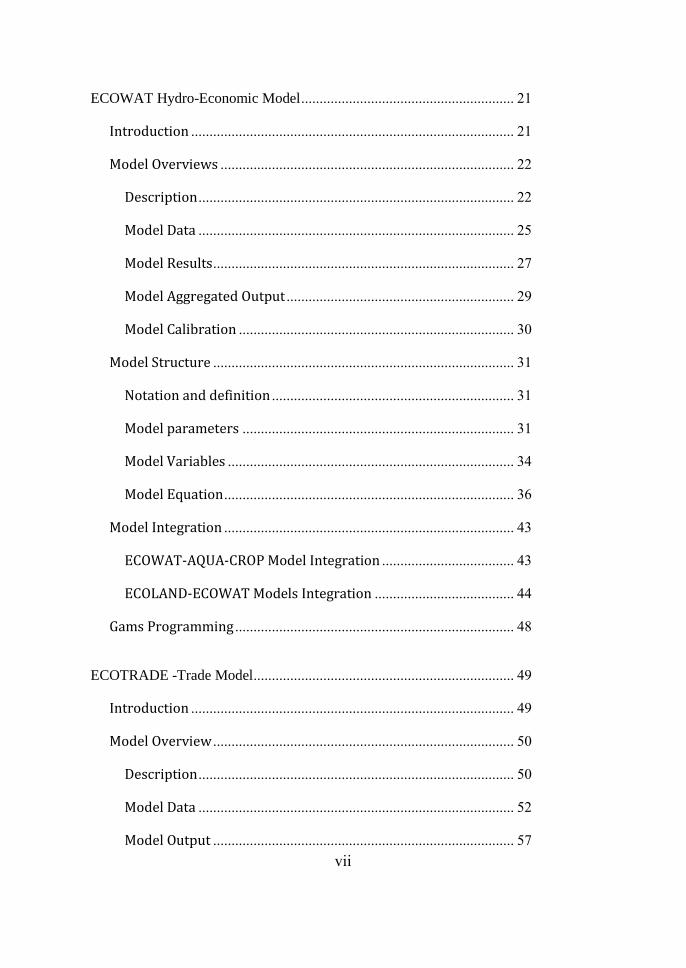
vii

ECOWAT Hydro-Economic Model .......................................................... 21

Introduction ........................................................................................ 21

Model Overviews ................................................................................ 22

Description ...................................................................................... 22

Model Data ...................................................................................... 25

Model Results .................................................................................. 27

Model Aggregated Output .............................................................. 29

Model Calibration ........................................................................... 30

Model Structure .................................................................................. 31

Notation and definition .................................................................. 31

Model parameters .......................................................................... 31

Model Variables .............................................................................. 34

Model Equation ............................................................................... 36

Model Integration ............................................................................... 43

ECOWAT-AQUA-CROP Model Integration .................................... 43

ECOLAND-ECOWAT Models Integration ...................................... 44

Gams Programming ............................................................................ 48

ECOTRADE -Trade Model ....................................................................... 49

Introduction ........................................................................................ 49

Model Overview .................................................................................. 50

Description ...................................................................................... 50

Model Data ...................................................................................... 52

Model Output .................................................................................. 57

viii

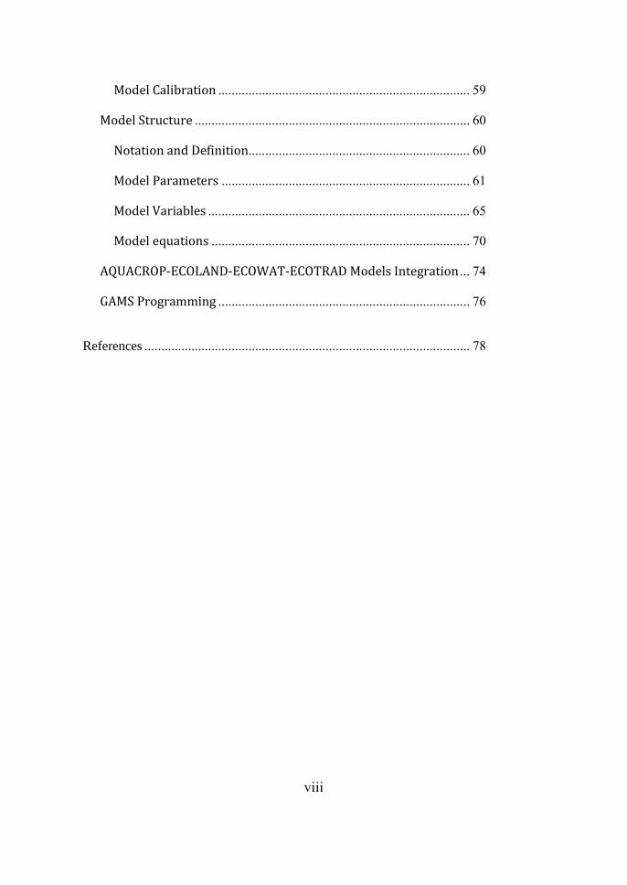
Model Calibration ........................................................................... 59

Model Structure .................................................................................. 60

Notation and Definition.................................................................. 60

Model Parameters .......................................................................... 61

Model Variables .............................................................................. 65

Model equations ............................................................................. 70

AQUACROP-ECOLAND-ECOWAT-ECOTRAD Models Integration ... 74

GAMS Programming ........................................................................... 76

References ................................................................................................. 78

ix

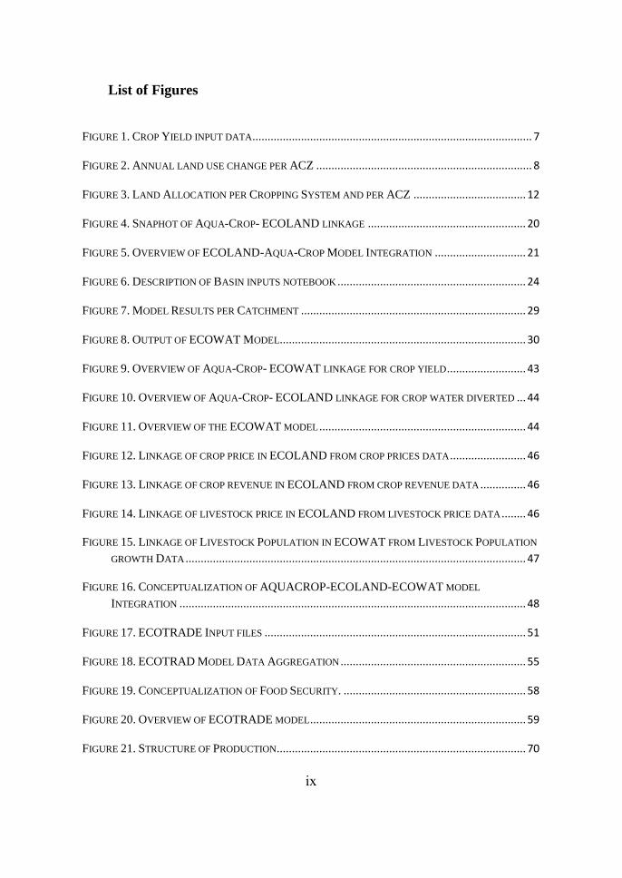
List of Figures

FIGURE 1. CROP YIELD INPUT DATA ............................................................................................ 7

FIGURE 2. ANNUAL LAND USE CHANGE PER ACZ ....................................................................... 8

FIGURE 3. LAND ALLOCATION PER CROPPING SYSTEM AND PER ACZ ..................................... 12

FIGURE 4. SNAPHOT OF AQUA-CROP- ECOLAND LINKAGE .................................................... 20

FIGURE 5. OVERVIEW OF ECOLAND-AQUA-CROP MODEL INTEGRATION .............................. 21

FIGURE 6. DESCRIPTION OF BASIN INPUTS NOTEBOOK .............................................................. 24

FIGURE 7. MODEL RESULTS PER CATCHMENT .......................................................................... 29

FIGURE 8. OUTPUT OF ECOWAT MODEL................................................................................. 30

FIGURE 9. OVERVIEW OF AQUA-CROP- ECOWAT LINKAGE FOR CROP YIELD .......................... 43

FIGURE 10. OVERVIEW OF AQUA-CROP- ECOLAND LINKAGE FOR CROP WATER DIVERTED ... 44

FIGURE 11. OVERVIEW OF THE ECOWAT MODEL .................................................................... 44

FIGURE 12. LINKAGE OF CROP PRICE IN ECOLAND FROM CROP PRICES DATA ......................... 46

FIGURE 13. LINKAGE OF CROP REVENUE IN ECOLAND FROM CROP REVENUE DATA ............... 46

FIGURE 14. LINKAGE OF LIVESTOCK PRICE IN ECOLAND FROM LIVESTOCK PRICE DATA ........ 46

FIGURE 15. LINKAGE OF LIVESTOCK POPULATION IN ECOWAT FROM LIVESTOCK POPULATION

GROWTH DATA ................................................................................................................ 47

FIGURE 16. CONCEPTUALIZATION OF AQUACROP-ECOLAND-ECOWAT MODEL

INTEGRATION .................................................................................................................. 48

FIGURE 17. ECOTRADE INPUT FILES ...................................................................................... 51

FIGURE 18. ECOTRAD MODEL DATA AGGREGATION ............................................................. 55

FIGURE 19. CONCEPTUALIZATION OF FOOD SECURITY. ............................................................ 58

FIGURE 20. OVERVIEW OF ECOTRADE MODEL ....................................................................... 59

FIGURE 21. STRUCTURE OF PRODUCTION .................................................................................. 70

x

FIGURE 22. COMMODITY TRADE FLOWS ................................................................................... 71

FIGURE 23. OVERVIEW OF AQUACROP-ECOLAND-ECOWAT-ECOTRAD MODELS

LINKAGE ......................................................................................................................... 76

xi

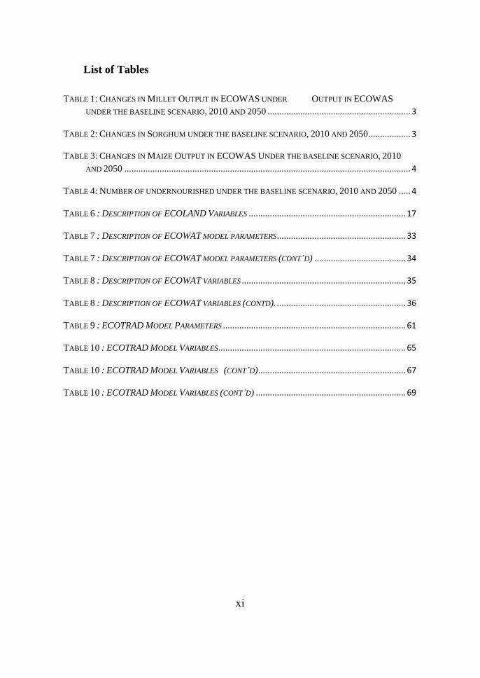
List of Tables

TABLE 1: CHANGES IN MILLET OUTPUT IN ECOWAS UNDER OUTPUT IN ECOWAS

UNDER THE BASELINE SCENARIO, 2010 AND 2050 ............................................................. 3

TABLE 2: CHANGES IN SORGHUM UNDER THE BASELINE SCENARIO, 2010 AND 2050 .................. 3

TABLE 3: CHANGES IN MAIZE OUTPUT IN ECOWAS UNDER THE BASELINE SCENARIO, 2010

AND 2050 .......................................................................................................................... 4

TABLE 4: NUMBER OF UNDERNOURISHED UNDER THE BASELINE SCENARIO, 2010 AND 2050 ..... 4

TABLE 6 : DESCRIPTION OF ECOLAND VARIABLES ................................................................... 17

TABLE 7 : DESCRIPTION OF ECOWAT MODEL PARAMETERS ....................................................... 33

TABLE 7 : DESCRIPTION OF ECOWAT MODEL PARAMETERS (CONT’D) ....................................... 34

TABLE 8 : DESCRIPTION OF ECOWAT VARIABLES ...................................................................... 35

TABLE 8 : DESCRIPTION OF ECOWAT VARIABLES (CONTD). ....................................................... 36

TABLE 9 : ECOTRAD MODEL PARAMETERS .............................................................................. 61

TABLE 10 : ECOTRAD MODEL VARIABLES ................................................................................ 65

TABLE 10 : ECOTRAD MODEL VARIABLES (CONT’D) ............................................................... 67

TABLE 10 : ECOTRAD MODEL VARIABLES (CONT’D) ................................................................ 69

1

General Introduction

There are no doubts that those extreme events such as drought and flood will

affect livelihoods in Sub-Sahara Africa (SSA), which includes the ECOWAS

Region. This is widely acknowledged by several studies, which explored the

impact of climate change across regions (FAO 2009; FAO, 2010; IPCC,

2014). Most analyses have concluded that the region is likely to be the most

vulnerable to climate change due to the fact that the economies of these

countries as agriculture depends primarily on rainfall. Agriculture is the

region’s key economic driving sector and the main employment generation

source. In addition, the sector contributes to foreign currency mobilization. It

has been predicted that the region’s’ crop productivity will change

significantly with some disparity among crop varieties. Claudia et al., (2010)

using IMPACT model found that in the Gulf of Guinea, by the year 2020, the

yield of rice and maize will increase by 1.80 and 2.40% respectively, while the

yield of sugarcane, cassava, and sweet potatoes will decrease by 0.50, 11.94

and 15.90% respectively. According to the same authors, following the

region’s growing population and structural changes, the region’s cereal

demand will increase from 145MT to 175 Mt while the demand for animal

products will increase from 8MT to 22MT between 2000 and 2050. This

changes coupled with climate change will transform the region into a net food

importer for only cereal crops. As a result, food commodity prices of maize,

wheat, and rice will increase by 34, 36 and 48% respectively between the year

2000 and 2050. Given the number of undernourished and food insecure people

in the region, this number will be expected to increase due to the reduction in

domestic food supply , increase in food prices and low household income.

Indeed, given the disparity among the production systems, agricultural

performance, agricultural policies and technology adoption of different

countries, the impact of climate change will significantly vary among

countries. Consequently, a disaggregated impact assessment is needed. In

order to achieve this, Nelson et al., (2010) explored the impact of climate

change among ECOWAS countries. This is illustrated in Tables 1 to 4 below.

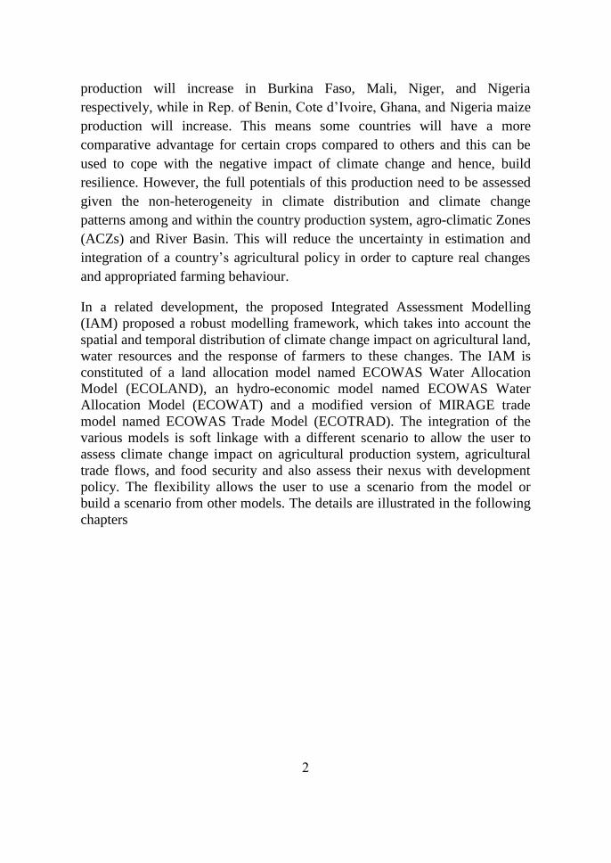
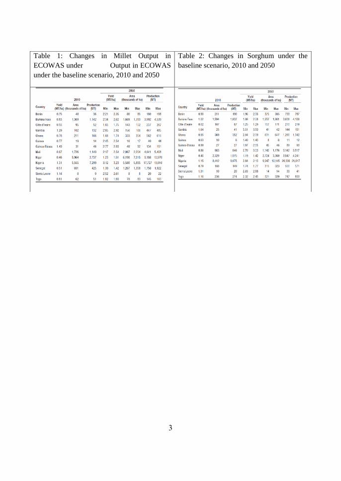
Analysis of Tables 1a, b and c showed that some countries will experience

increase in their grain production while others will experience a decrease in

their grain production. According to these results, millet and sorghum

2

production will increase in Burkina Faso, Mali, Niger, and Nigeria

respectively, while in Rep. of Benin, Cote d’Ivoire, Ghana, and Nigeria maize

production will increase. This means some countries will have a more

comparative advantage for certain crops compared to others and this can be

used to cope with the negative impact of climate change and hence, build

resilience. However, the full potentials of this production need to be assessed

given the non-heterogeneity in climate distribution and climate change

patterns among and within the country production system, agro-climatic Zones

(ACZs) and River Basin. This will reduce the uncertainty in estimation and

integration of a country’s agricultural policy in order to capture real changes

and appropriated farming behaviour.

In a related development, the proposed Integrated Assessment Modelling

(IAM) proposed a robust modelling framework, which takes into account the

spatial and temporal distribution of climate change impact on agricultural land,

water resources and the response of farmers to these changes. The IAM is

constituted of a land allocation model named ECOWAS Water Allocation

Model (ECOLAND), an hydro-economic model named ECOWAS Water

Allocation Model (ECOWAT) and a modified version of MIRAGE trade

model named ECOWAS Trade Model (ECOTRAD). The integration of the

various models is soft linkage with a different scenario to allow the user to

assess climate change impact on agricultural production system, agricultural

trade flows, and food security and also assess their nexus with development

policy. The flexibility allows the user to use a scenario from the model or

build a scenario from other models. The details are illustrated in the following

chapters

3

Table 1: Changes in Millet Output in

ECOWAS under Output in ECOWAS

under the baseline scenario, 2010 and 2050

Table 2: Changes in Sorghum under the

baseline scenario, 2010 and 2050

4

Table 3: Changes in Maize Output in

ECOWAS Under the baseline scenario, 2010

and 2050

Table 4: Number of undernourished under

the baseline scenario, 2010 and 2050

ECOLAND - Land Allocation Model

Introduction The land allocation model (or ECOLAND) is a dynamic intertemporal and

spatial ECOWAS whole farm model. It is a modified version of the

“AGRESTE” whole farm model (Kutcher and Scandizzo, 1981). The

representative risk-neutral and profit maximization agent operates in an agro-

climatic zone (ACZ) as units and there are 39 of these. The farming system is

characterized by seven (7) cropping systems mainly paddy rice (pdr); cereal

(gro), vegetable –fruit-nuts (av_f); oil seeds (osd); sugarcane-sugarbeet (c_b),

fibers (pfb) and indigenous crops (ocr). This is akin to the Global Trade

Analysis Project (GTAP) classification of crops and four (4) livestock

breeding systems mainly cattle, sheep, chicken and others.

5

The model aims to estimate the corresponding land allocation for each

agricultural crop and a group of crops in each given ACZ from year 2004 up to

year 2100 with respect to climate change. It uses the theory of representative

risk-neutral farm agent producing food crop and rearing livestock. In this

model, agricultural crops and livestock activities that are appropriate are

considered for each of these ACZs. The farm agent objective is to optimize the

farming profit. This is illustrated by Max (yfarm), where yfarm is the sum of

income made from crop production, and livestock minus all production costs

such as cropping activity cost, labour cost definition, working capital

requirements, veterinary costs, and technology adoption costs. However, the

profit maximization is subject to resource constraints. This includes arable

land, labour, fertilizer, seeds, and other relevant input and their costs. The

decision-making of the economic agent will consist of adequately allocating

available resources to sustain the business of farmers. Thus, the estimation of

the appropriate land use in each ACZ and how it will perform under the whole

farm model.

Model Overviews

Description

The model is an ACZ unit based model. Each ACZ input data relative to the

year 2004 is located in the workbook called “ECOLANDNEW.XLX”, which

was linked to another file called ECOCALIB.GMS. The latter performs the

optimization for the baseline. As for the simulation data (from year 2010 to

2100), twelve workbooks were used and some of these are

“ECOLANDNEW45SSP1-ECOLANDNEW45SSP4, ECOLANDNEW85SSP1 -

ECOLANDNEW85SSP4, ECOLANDNEWSSP1 - ECOLANDNEWSSP4”.

Indeed, the model included two climate- change scenarios (Representative

6

Concentration Pathways-RCPs 4.5 and 8.5), and four socio-economic

scenarios (Share Socio-economic Pathways-SSPs) (Vervoort et al., 2013).

Each RCP was combined with the SSP files. Consequently, there were eight

(8) scenarios with climate change and four additional scenarios without

climate change. For example, ECOLANDNEW45SSP1 refers to the

combination of the RCP4.5 with the SSP1 and ECOLANDNEWSSP4 is

relative to SSP1 without accounting for climate change.

Model Data

Data used were from several sources, and these included desk review and

collection of socio-economic data. Indeed, socioeconomic parameters used in

the modeling were from e.g., Louhichi et al(2013); Louhichi &

Paloma(2014); Lokonon et al( 2015); Yilma( 2006); Kutcher &

Scandizzo(1981); Paloma et al.(2012). Other sources include World

Development Institute Database and the Food and Agriculture Organization

(FAO) database. The base year data is 2010 while projection has been made

up to 2100.

Climate data:

The ECOLAND climate data was represented by cropping yield. This was

defined for three (3) levels following three (3) RCP scenarios. However, crop

yield data were obtained from AQUA-CROP model, which uses climate and

crop management data (AQU-CROP, 20xxx). ECOLAND climate data are

linked to crop yields. This was defined for two (2) levels following two (2)

RCP scenarios. However, crop yields can be simulated also through AQUA-

CROP model, which needs climate data and crop- management data, or this

may be calibrated through a multi-regression approach (econometric

7

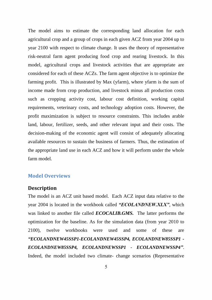
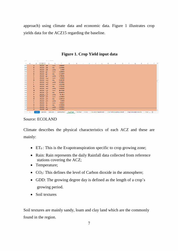
approach) using climate data and economic data. Figure 1 illustrates crop

yields data for the ACZ15 regarding the baseline.

Figure 1. Crop Yield input data

Source: ECOLAND

Climate describes the physical characteristics of each ACZ and these are

mainly:

ET0 : This is the Evapotranspiration specific to crop growing zone;

Rain: Rain represents the daily Rainfall data collected from reference

stations covering the ACZ;

Temperature;

CO2: This defines the level of Carbon dioxide in the atmosphere;

GDD: The growing degree day is defined as the length of a crop’s

growing period.

Soil textures

Soil textures are mainly sandy, loam and clay land which are the commonly

found in the region.

8

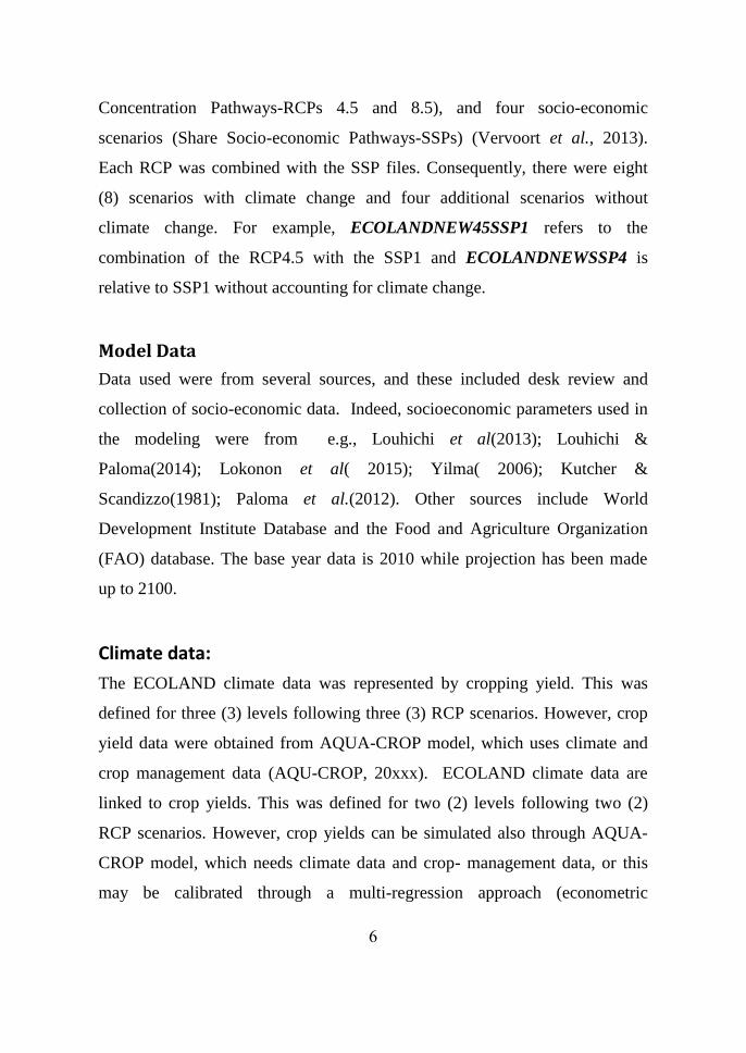
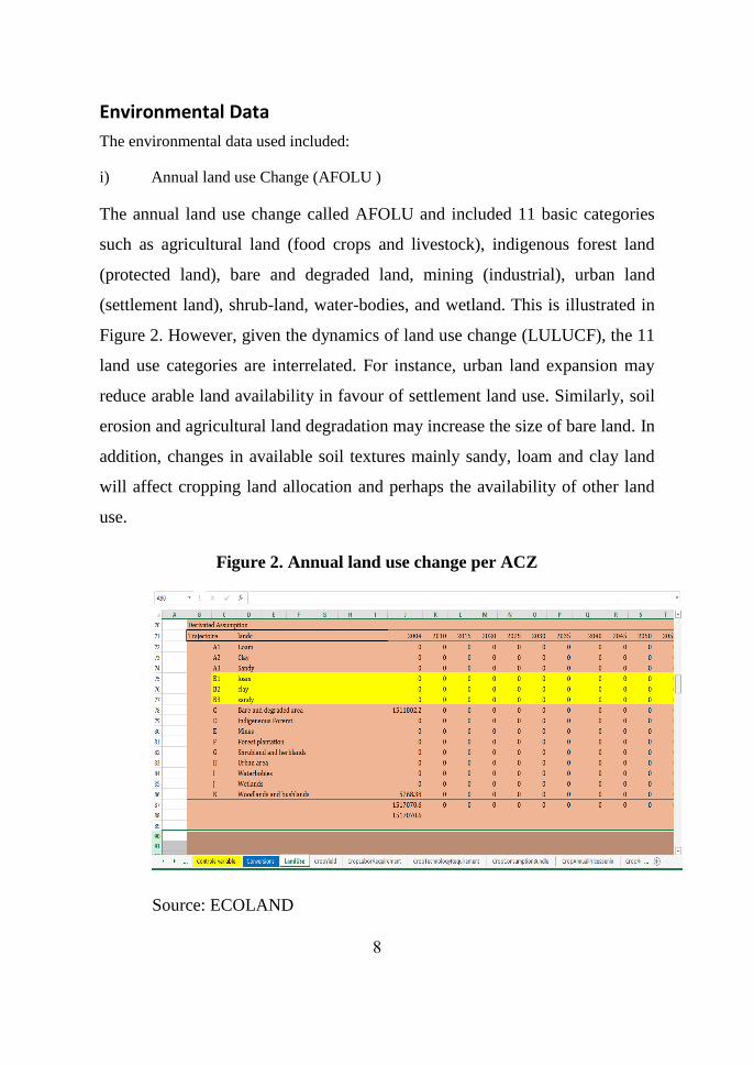
Environmental Data

The environmental data used included:

i) Annual land use Change (AFOLU )

The annual land use change called AFOLU and included 11 basic categories

such as agricultural land (food crops and livestock), indigenous forest land

(protected land), bare and degraded land, mining (industrial), urban land

(settlement land), shrub-land, water-bodies, and wetland. This is illustrated in

Figure 2. However, given the dynamics of land use change (LULUCF), the 11

land use categories are interrelated. For instance, urban land expansion may

reduce arable land availability in favour of settlement land use. Similarly, soil

erosion and agricultural land degradation may increase the size of bare land. In

addition, changes in available soil textures mainly sandy, loam and clay land

will affect cropping land allocation and perhaps the availability of other land

use.

Figure 2. Annual land use change per ACZ

Source: ECOLAND

9

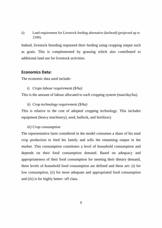
ii) Land requirement for Livestock feeding alternative (ha/head) (projected up to

2100).

Indeed, livestock breeding requested their feeding using cropping output such

as grain. This is complemented by grassing which also contributed to

additional land use for livestock activities.

Economics Data:

The economic data used include:

i) Crops labour requirement ($/ha)

This is the amount of labour allocated to each cropping system (man/day/ha).

ii) Crop technology requirement ($/ha)

This is relative to the cost of adopted cropping technology. This includes

equipment (heavy machinery), seed, bullock, and fertilizer).

iii) Crop consumption

The representative farm considered in the model consumes a share of his total

crop production to feed his family and sells the remaining output in the

market. This consumption constitutes a level of household consumption and

depends on their food consumption demand. Based on adequacy and

appropriateness of their food consumption for meeting their dietary demand,

three levels of household food consumption are defined and these are: (i) for

low consumption, (ii) for more adequate and appropriated food consumption

and (iii) is for highly better- off class.

10

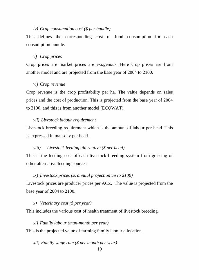
iv) Crop consumption cost ($ per bundle)

This defines the corresponding cost of food consumption for each

consumption bundle.

v) Crop prices

Crop prices are market prices are exogenous. Here crop prices are from

another model and are projected from the base year of 2004 to 2100.

vi) Crop revenue

Crop revenue is the crop profitability per ha. The value depends on sales

prices and the cost of production. This is projected from the base year of 2004

to 2100, and this is from another model (ECOWAT).

vii) Livestock labour requirement

Livestock breeding requirement which is the amount of labour per head. This

is expressed in man-day per head.

viii) Livestock feeding alternative ($ per head)

This is the feeding cost of each livestock breeding system from grassing or

other alternative feeding sources.

ix) Livestock prices ($, annual projection up to 2100)

Livestock prices are producer prices per ACZ. The value is projected from the

base year of 2004 to 2100.

x) Veterinary cost ($ per year)

This includes the various cost of health treatment of livestock breeding.

xi) Family labour (man-month per year)

This is the projected value of farming family labour allocation.

xii) Family wage rate ($ per month per year)

11

The family labour use can also be remunerated following their time allocation

in farming activities. This is projected from the base year of 2004 to 2100.

xiii) Farming population

Farming population is the total number of people directly involved in

agricultural activities from land preparation to harvesting.

xiv) Temporal wage rate

This is relative to the wage rate for hired labour that is supposed to work

temporarily on the farm.

xv) Permanent wage rate

This is relative to the wage rate for hired labour that is supposed to work

permanently on the farm.

xvi) Working capital requirement ($)

It accounts for the total amount available for farming activities.

12

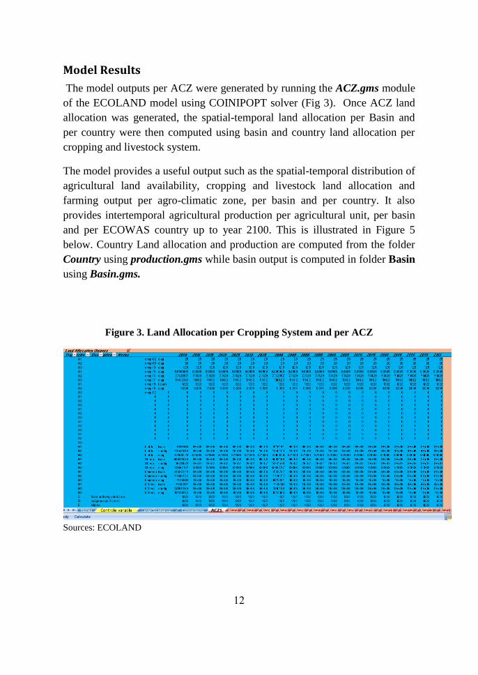
Model Results

The model outputs per ACZ were generated by running the ACZ.gms module

of the ECOLAND model using COINIPOPT solver (Fig 3). Once ACZ land

allocation was generated, the spatial-temporal land allocation per Basin and

per country were then computed using basin and country land allocation per

cropping and livestock system.

The model provides a useful output such as the spatial-temporal distribution of

agricultural land availability, cropping and livestock land allocation and

farming output per agro-climatic zone, per basin and per country. It also

provides intertemporal agricultural production per agricultural unit, per basin

and per ECOWAS country up to year 2100. This is illustrated in Figure 5

below. Country Land allocation and production are computed from the folder

Country using production.gms while basin output is computed in folder Basin

using Basin.gms.

Figure 3. Land Allocation per Cropping System and per ACZ

Sources: ECOLAND

13

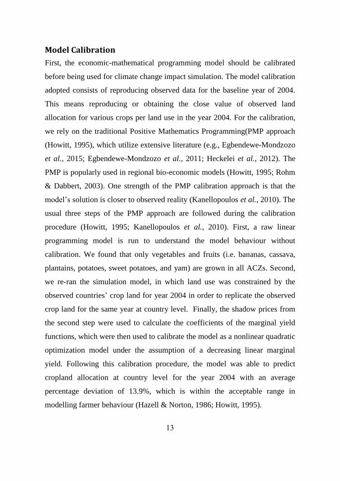
Model Calibration

First, the economic-mathematical programming model should be calibrated

before being used for climate change impact simulation. The model calibration

adopted consists of reproducing observed data for the baseline year of 2004.

This means reproducing or obtaining the close value of observed land

allocation for various crops per land use in the year 2004. For the calibration,

we rely on the traditional Positive Mathematics Programming(PMP approach

(Howitt, 1995), which utilize extensive literature (e.g., Egbendewe-Mondzozo

et al., 2015; Egbendewe-Mondzozo et al., 2011; Heckelei et al., 2012). The

PMP is popularly used in regional bio-economic models (Howitt, 1995; Rohm

& Dabbert, 2003). One strength of the PMP calibration approach is that the

model’s solution is closer to observed reality (Kanellopoulos et al., 2010). The

usual three steps of the PMP approach are followed during the calibration

procedure (Howitt, 1995; Kanellopoulos et al., 2010). First, a raw linear

programming model is run to understand the model behaviour without

calibration. We found that only vegetables and fruits (i.e. bananas, cassava,

plantains, potatoes, sweet potatoes, and yam) are grown in all ACZs. Second,

we re-ran the simulation model, in which land use was constrained by the

observed countries’ crop land for year 2004 in order to replicate the observed

crop land for the same year at country level. Finally, the shadow prices from

the second step were used to calculate the coefficients of the marginal yield

functions, which were then used to calibrate the model as a nonlinear quadratic

optimization model under the assumption of a decreasing linear marginal

yield. Following this calibration procedure, the model was able to predict

cropland allocation at country level for the year 2004 with an average

percentage deviation of 13.9%, which is within the acceptable range in

modelling farmer behaviour (Hazell & Norton, 1986; Howitt, 1995).

14

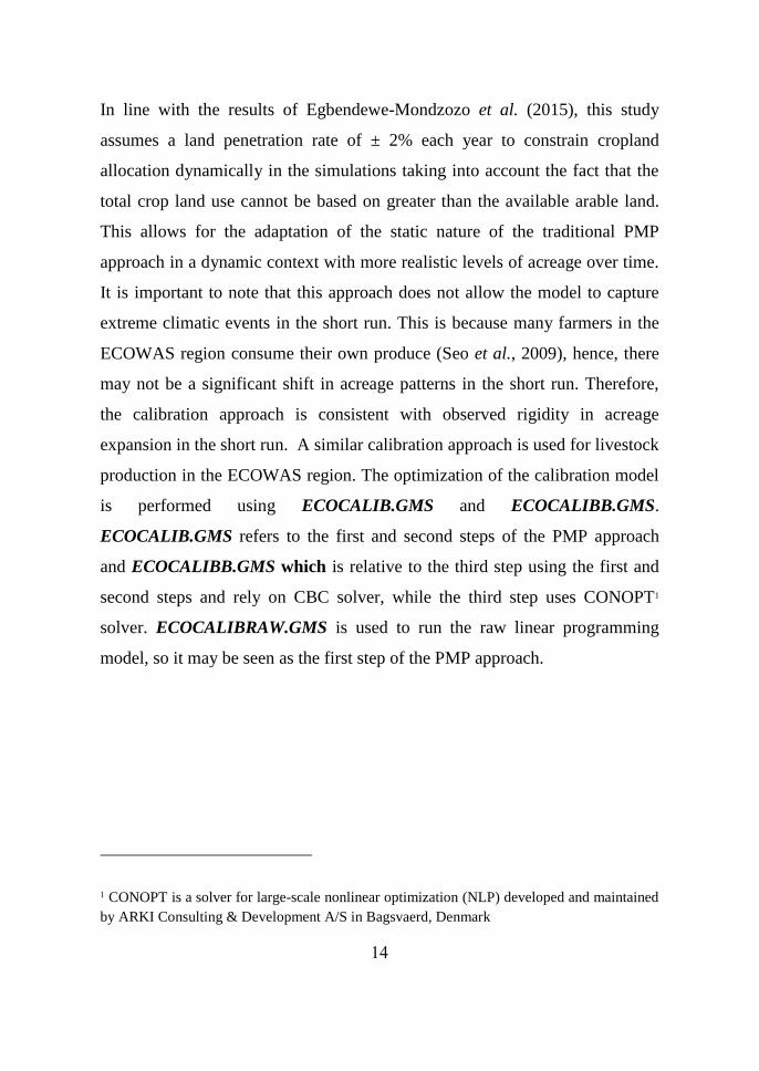
In line with the results of Egbendewe-Mondzozo et al. (2015), this study

assumes a land penetration rate of ± 2% each year to constrain cropland

allocation dynamically in the simulations taking into account the fact that the

total crop land use cannot be based on greater than the available arable land.

This allows for the adaptation of the static nature of the traditional PMP

approach in a dynamic context with more realistic levels of acreage over time.

It is important to note that this approach does not allow the model to capture

extreme climatic events in the short run. This is because many farmers in the

ECOWAS region consume their own produce (Seo et al., 2009), hence, there

may not be a significant shift in acreage patterns in the short run. Therefore,

the calibration approach is consistent with observed rigidity in acreage

expansion in the short run. A similar calibration approach is used for livestock

production in the ECOWAS region. The optimization of the calibration model

is performed using ECOCALIB.GMS and ECOCALIBB.GMS.

ECOCALIB.GMS refers to the first and second steps of the PMP approach

and ECOCALIBB.GMS which is relative to the third step using the first and

second steps and rely on CBC solver, while the third step uses CONOPT1

solver. ECOCALIBRAW.GMS is used to run the raw linear programming

model, so it may be seen as the first step of the PMP approach.

1 CONOPT is a solver for large-scale nonlinear optimization (NLP) developed and maintained

by ARKI Consulting & Development A/S in Bagsvaerd, Denmark

15

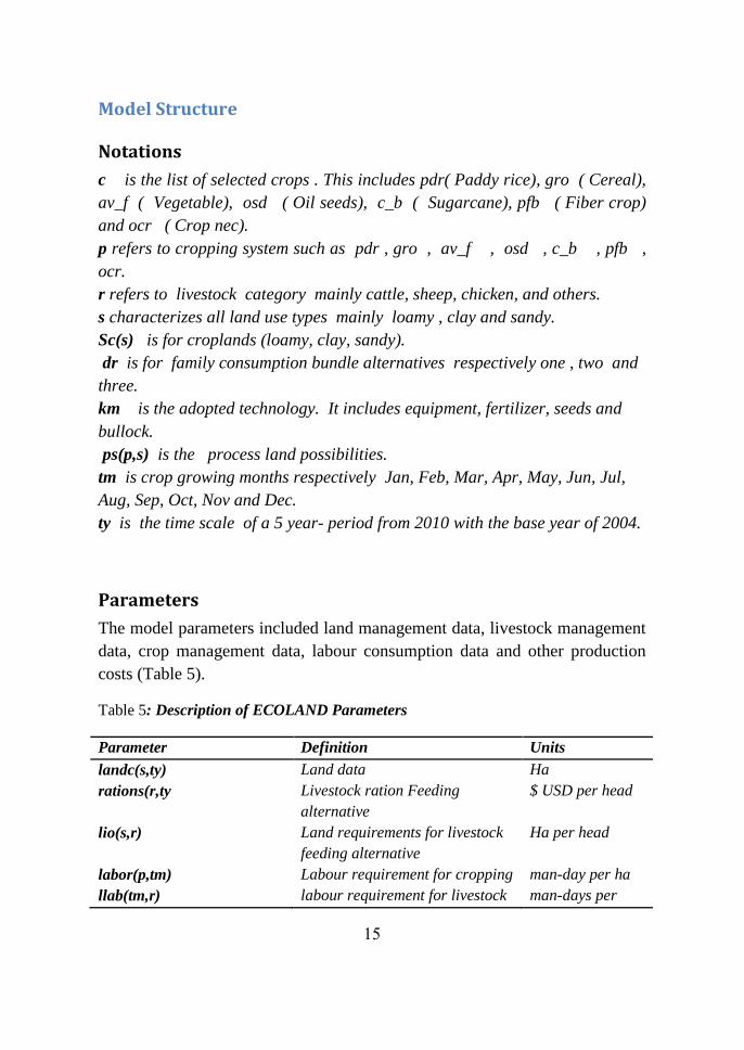
Model Structure

Notations

c is the list of selected crops . This includes pdr( Paddy rice), gro ( Cereal),

av_f ( Vegetable), osd ( Oil seeds), c_b ( Sugarcane), pfb ( Fiber crop)

and ocr ( Crop nec).

p refers to cropping system such as pdr , gro , av_f , osd , c_b , pfb ,

ocr.

r refers to livestock category mainly cattle, sheep, chicken, and others.

s characterizes all land use types mainly loamy , clay and sandy.

Sc(s) is for croplands (loamy, clay, sandy).

dr is for family consumption bundle alternatives respectively one , two and

three.

km is the adopted technology. It includes equipment, fertilizer, seeds and

bullock.

ps(p,s) is the process land possibilities.

tm is crop growing months respectively Jan, Feb, Mar, Apr, May, Jun, Jul,

Aug, Sep, Oct, Nov and Dec.

ty is the time scale of a 5 year- period from 2010 with the base year of 2004.

Parameters

The model parameters included land management data, livestock management

data, crop management data, labour consumption data and other production

costs (Table 5).

Table 5: Description of ECOLAND Parameters

Parameter Definition Units

landc(s,ty) Land data Ha

rations(r,ty Livestock ration Feeding

alternative

$ USD per head

lio(s,r) Land requirements for livestock

feeding alternative

Ha per head

labor(p,tm) Labour requirement for cropping man-day per ha

llab(tm,r) labour requirement for livestock man-days per

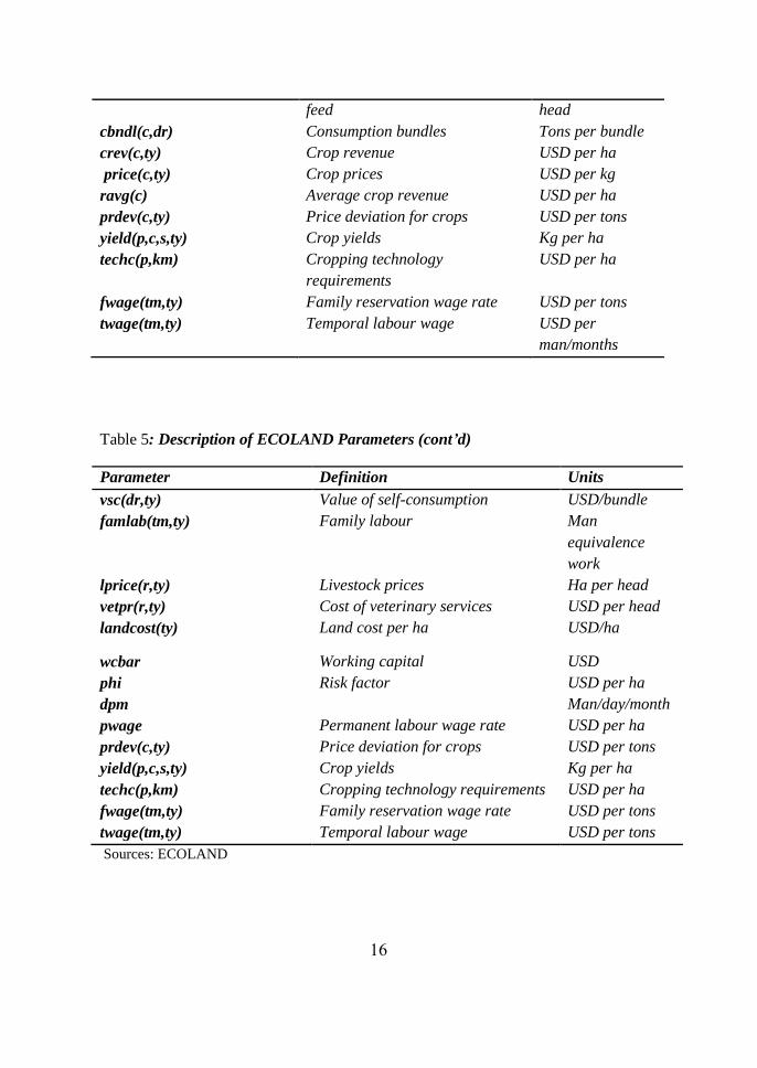
16

feed head

cbndl(c,dr) Consumption bundles Tons per bundle

crev(c,ty) Crop revenue USD per ha

price(c,ty) Crop prices USD per kg

ravg(c) Average crop revenue USD per ha

prdev(c,ty) Price deviation for crops USD per tons

yield(p,c,s,ty) Crop yields Kg per ha

techc(p,km) Cropping technology

requirements

USD per ha

fwage(tm,ty) Family reservation wage rate USD per tons

twage(tm,ty) Temporal labour wage USD per

man/months

Table 5: Description of ECOLAND Parameters (cont’d)

Parameter Definition Units

vsc(dr,ty) Value of self-consumption USD/bundle

famlab(tm,ty) Family labour Man

equivalence

work

lprice(r,ty) Livestock prices Ha per head

vetpr(r,ty) Cost of veterinary services USD per head

landcost(ty) Land cost per ha USD/ha

wcbar Working capital USD

phi Risk factor USD per ha

dpm Man/day/month

pwage Permanent labour wage rate USD per ha

prdev(c,ty) Price deviation for crops USD per tons

yield(p,c,s,ty) Crop yields Kg per ha

techc(p,km) Cropping technology requirements USD per ha

fwage(tm,ty) Family reservation wage rate USD per tons

twage(tm,ty) Temporal labour wage USD per tons

Sources: ECOLAND

17

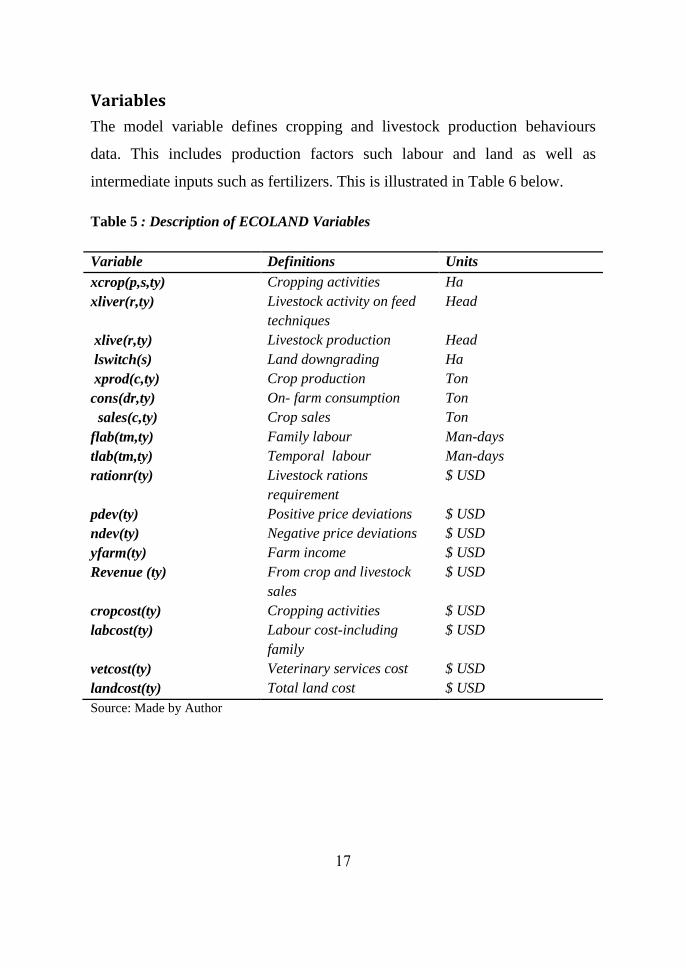
Variables

The model variable defines cropping and livestock production behaviours

data. This includes production factors such labour and land as well as

intermediate inputs such as fertilizers. This is illustrated in Table 6 below.

Table 5 : Description of ECOLAND Variables

Variable Definitions Units

xcrop(p,s,ty) Cropping activities Ha

xliver(r,ty) Livestock activity on feed

techniques

Head

xlive(r,ty) Livestock production Head

lswitch(s) Land downgrading Ha

xprod(c,ty) Crop production Ton

cons(dr,ty) On- farm consumption Ton

sales(c,ty) Crop sales Ton

flab(tm,ty) Family labour Man-days

tlab(tm,ty) Temporal labour Man-days

rationr(ty) Livestock rations

requirement

$ USD

pdev(ty) Positive price deviations $ USD

ndev(ty) Negative price deviations $ USD

yfarm(ty) Farm income $ USD

Revenue (ty) From crop and livestock

sales

$ USD

cropcost(ty) Cropping activities $ USD

labcost(ty) Labour cost-including

family

$ USD

vetcost(ty) Veterinary services cost $ USD

landcost(ty) Total land cost $ USD

Source: Made by Author

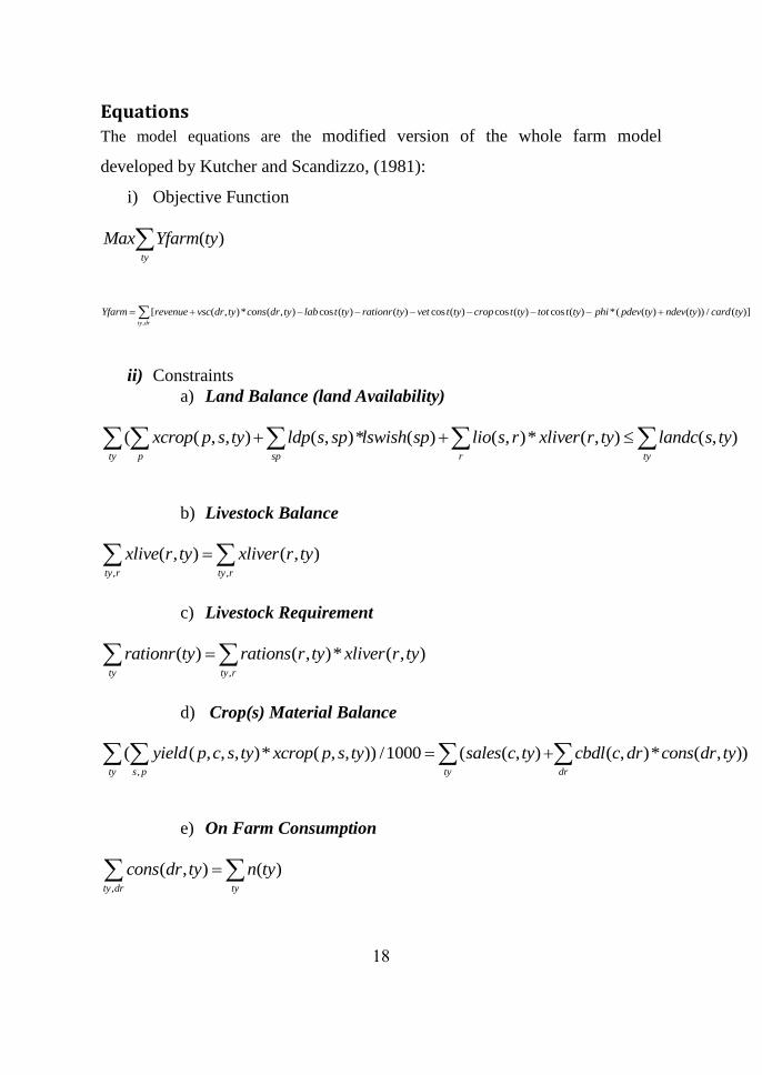
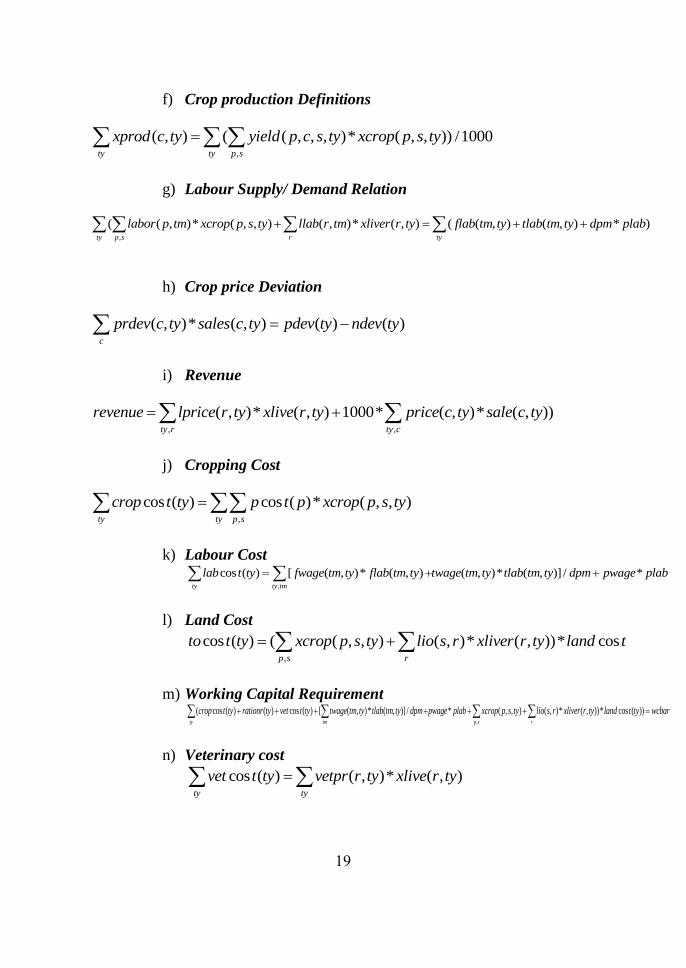
18

Equations The model equations are the modified version of the whole farm model

developed by Kutcher and Scandizzo, (1981):

i) Objective Function

( )ty

Max Yfarm ty

,

[ ( , )* ( , ) cos ( ) ( ) cos ( ) cos ( ) cos ( ) *( ( ) ( )) / ( )]ty dr

Yfarm revenue vsc dr ty cons dr ty lab t ty rationr ty vet t ty crop t ty tot t ty phi pdev ty ndev ty card ty

ii) Constraints

a) Land Balance (land Availability)

( ( , , ) ( , )* ( ) ( , )* ( , ) ( , )ty p sp r ty

xcrop p s ty ldp s sp lswish sp lio s r xliver r ty landc s ty

b) Livestock Balance

, ,

( , ) ( , )ty r ty r

xlive r ty xliver r ty

c) Livestock Requirement

,

( ) ( , )* ( , )ty ty r

rationr ty rations r ty xliver r ty

d) Crop(s) Material Balance

,

( ( , , , )* ( , , )) /1000 ( ( , ) ( , )* ( , ))ty s p ty dr

yield p c s ty xcrop p s ty sales c ty cbdl c dr cons dr ty

e) On Farm Consumption

,

( , ) ( )ty dr ty

cons dr ty n ty

19

f) Crop production Definitions

,

( , ) ( ( , , , )* ( , , )) /1000ty ty p s

xprod c ty yield p c s ty xcrop p s ty

g) Labour Supply/ Demand Relation

,

( ( , )* ( , , ) ( , )* ( , ) ( ( , ) ( , ) * )ty p s r ty

labor p tm xcrop p s ty llab r tm xliver r ty flab tm ty tlab tm ty dpm plab

h) Crop price Deviation

( , )* ( , ) ( ) ( )c

prdev c ty sales c ty pdev ty ndev ty

i) Revenue

, ,

( , )* ( , ) 1000* ( , )* ( , ))ty r ty c

revenue lprice r ty xlive r ty price c ty sale c ty

j) Cropping Cost

,

cos ( ) cos ( )* ( , , )ty ty p s

crop t ty p t p xcrop p s ty

k) Labour Cost

,

cos ( ) [ ( , )* ( , ) ( , )* ( , )] / *ty ty tm

lab t ty fwage tm ty flab tm ty twage tm ty tlab tm ty dpm pwage plab

l) Land Cost

,

cos ( ) ( ( , , ) ( , )* ( , ))* cosp s r

to t ty xcrop p s ty lio s r xliver r ty land t

m) Working Capital Requirement

,

( cos ( ) ( ) cos ( ) [ ( , )* ( , )] / * ( , , ) ( , )* ( , ))* cos ( ))ty tm p s r

crop t ty rationr ty vet t ty twage tm ty tlab tm ty dpm pwage plab xcrop p s ty lio s r xliver r ty land t ty wcbar

n) Veterinary cost

cos ( ) ( , )* ( , )ty ty

vet t ty vetpr r ty xlive r ty

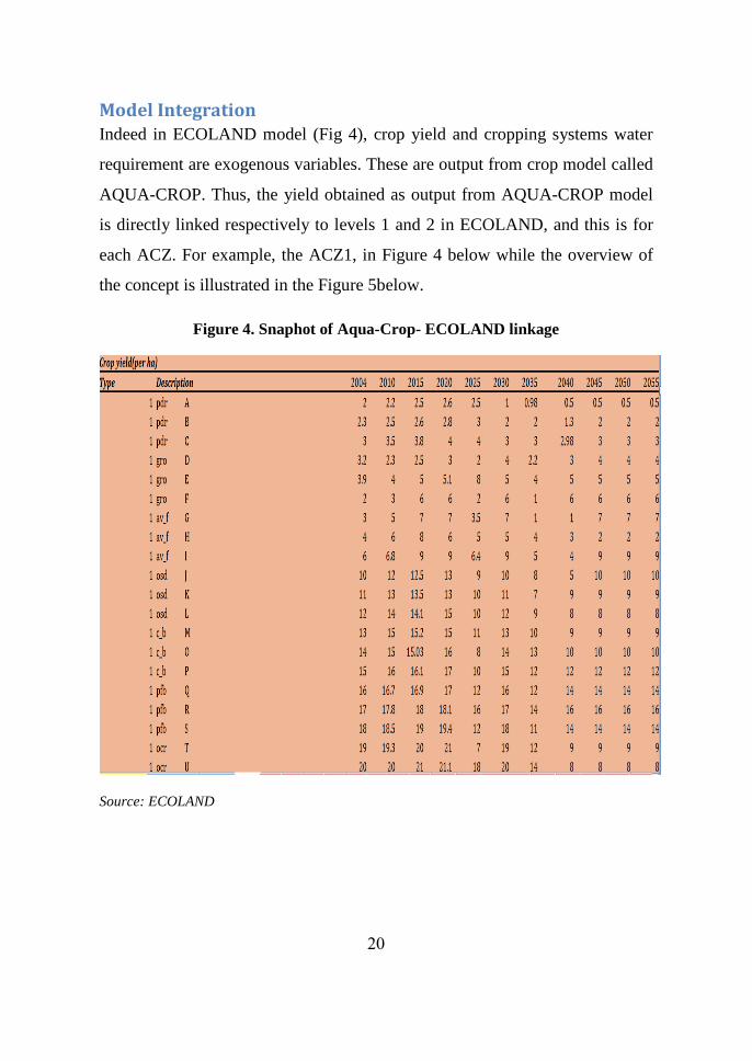
20

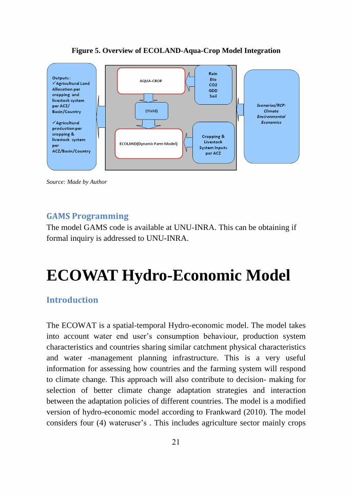
Model Integration Indeed in ECOLAND model (Fig 4), crop yield and cropping systems water

requirement are exogenous variables. These are output from crop model called

AQUA-CROP. Thus, the yield obtained as output from AQUA-CROP model

is directly linked respectively to levels 1 and 2 in ECOLAND, and this is for

each ACZ. For example, the ACZ1, in Figure 4 below while the overview of

the concept is illustrated in the Figure 5below.

Figure 4. Snaphot of Aqua-Crop- ECOLAND linkage

Source: ECOLAND

21

Figure 5. Overview of ECOLAND-Aqua-Crop Model Integration

Source: Made by Author

GAMS Programming

The model GAMS code is available at UNU-INRA. This can be obtaining if

formal inquiry is addressed to UNU-INRA.

ECOWAT Hydro-Economic Model

Introduction

The ECOWAT is a spatial-temporal Hydro-economic model. The model takes

into account water end user’s consumption behaviour, production system

characteristics and countries sharing similar catchment physical characteristics

and water -management planning infrastructure. This is a very useful

information for assessing how countries and the farming system will respond

to climate change. This approach will also contribute to decision- making for

selection of better climate change adaptation strategies and interaction

between the adaptation policies of different countries. The model is a modified

version of hydro-economic model according to Frankward (2010). The model

considers four (4) wateruser’s . This includes agriculture sector mainly crops

22

and livestock; household; hydro-power production and recreation water users

for five of the major Basin system (i.e. the Niger Basin, Senegal Basin, Volta

Basin, Gambia Basin and Lake Chad. It should be noted that the ECOWAS or

(West African) region is characterized by trans-boundary Catchment. The

model has included two cropping seasons of rainfall season starting from

March to September and drought season starting from October to February and

during the latter, the fields are irrigated. This is to capture the tradeoff of water

usage between rainfed cropping system and irrigation system. The model is set

up with time scale up to the year 2100. The model aims to optimize the total

benefit of water usage in each catchment. This is expressed by

MaxTot_ben_v(p,s) where Tot_ben_v(p,s) is basically the sum of the benefits

of basin related water usage activities. This includes:

Ag_ben_v(use,y,t,p,s) for agricultural benefit ;

ben_s(res,y,t,p )for recreation benefit ;

m_ben_v(use,y,t,p,s) for livestock breeding benefit ;

Energy_ben(res,hydro,t,p,s) for hydro-electricity benefit ;and

U_benefit_uV(use,y,t,p,s) for household water usage benefit .

The model computes optimal output such as inter-temporal crop revenue,

crop price, cropping land allocation and water allocation in decision-

making to maximize catchment water usage benefit among end users.

Model Overviews

Description

The model is a catchment based model. For each catchment, it uses a

catchment input data named “Basinname.B.xls” which is linked to a GAMS

programming code called watmodel.gms. The “Basinname.B.xls” is an excel

workbook made of 29 excel sheets describing the catchment geometry and end

user of water data. For example, for Niger Basin, input data are included in

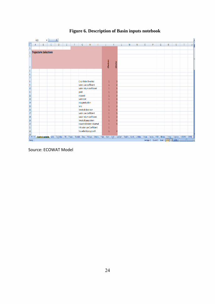
NigerB.xls. This is illustrated in Figure 6 below where:

23

Control variable is scenario definition sheet

Sets include notation and definitions;

In _Index is the link option between NigerB.xls and watmodel.gms;

VB contain basin geometry table and reservoir linkage;

Flows define Volta basin inflows data;

Rainfall defines rainfall data;

Bwu contains agricultural crop water diverted data;

Wtuse describes agricultural water- use efficiency;

Wretu describes the level of water return into the basin system after crop

irrigation;

Yield contains crop yield data per ACZ;

Cost defines crop production cost per ACZ;

Q_p defines crop total production per ACZ;

Wcost defines cropping system water cost per ACZ;

ResEn defines hydro-energy data base;

Land defines land use database per ACZ;

UrbUse defines household water usage data include in both urban and rural

household per ACZ;

Htuse contains urban water efficiency per ACZ;

Hrute expresses the level of household water return into the basin per ACZ;

Pop defines household population per ACZ;

Hhsize defines household size per ACZ;

Hmag household water spending per per ACZ;

Urprice defines household water price;

HGROW defines household population growth per ACZ;

LIVD expresses livestock water diverted per ACZ;

mtuse livestock industry water- use efficiency per ACZ;

mretu contain data on livestock breeding water return per ACZ;

mpop contains livestock population per ACZ;

Qm contains livestock production for the base year per ACZ;

MGROW contains information on livestock population growth per ACZ;

24

Figure 6. Description of Basin inputs notebook

Source: ECOWAT Model

25

Model Data

Model inputs are per ACZ and are related to climate, economies, and

environments. This includes climate data, cropping system inputs, livestock

breeding inputs, hydro-electricity production data and household water usage

data.

Climate data:

Here, climate data are mainly physical data and describe the catchment

hydrology:

i) Rainfall

This is the quantified amount of precipitation in the selected catchment. It is

expressed in m3. This is the evapotranspiration in selected catchment

ii) Flow

This is a function of rainfall, sub-catchment area, the runoff and

level of ground water recharge. This is expressed in the following

equation:

_ (inf , , , ) ( * )source p low y t s P S ETo Rainoff Grw Where:

P is the rainfall

S : the area of each sub-catchment (inflow)

is the evapotranspiration

iii) Grw is ground water recharge

Cropping system

i) Crop water use per agro-climatic zone

Crop water use is a share of diverted water from inflow source which is used

really by planting material during the growing period. This is expressed by:

26

( , , , ) ( , , )* ( _ ( , )* ( , , , ))divert

Bu use j t z wtuse use t z ID ud use divert Bu divert j t z

ii) Wtuse (use,t,z) water use coefficient per agro -climatic zone

This represents crop water use efficiency. It may vary by ACZ depending on

farmer’s water usage.

iii) Water return

One water is diverted from sources and the crop water requirement is met; the

remaining water is returned into the system. This is expressed by

( , , , ) ( , , )* ( _ ( , )* ( , , , ))return

Bu return j t z wretu use t z ID ud return divert Bu divert j t z

iv) Wretu (return,t,z) water return coefficient per agro-climatic

zone

v) Yield_p(use,j,k,z) Crop Yield tons per acre (proportional to ET

when technology varies)

vi) Price_p(j) Crop Prices ($ per ton)

vii) Cost_p(use,j,k,z) Crop Production Costs ($ per acre)

viii) wcost_p(use,j,k,z) crop water cost($ per acre)

ix) Q_p(use,j,z) crop production

x) price_elast(j) crop prices elasticity

xi) landrhs_p(use,y,z) land in production

Household

i) mu_use_base_p(i,l,t,z) base water delivery (acre feet/hh/year)

ii) htuse(use,t,z) hh water use coefficient

iii) hretu(return,t,z) hh water return coefficient

iv) pop(use,l,t,z) urban and rural pop (1000s of households)

v) Hhsize(use,l,t,z) hh size

vi) hhgrowth(use,l,y,t,z) hh pop annual growth rate

27

vii) p_elasticity_p(use,l,t) price elasticity of demand for water

viii) mu_price_base_p(use,l,t,z) base year hh water price ($ per

acre foot)

ix) AC_uuse0_p(use,l,t,z) base year marginal cost of supply.

Livestock

i) mbase_p(i,m,t,z) total livestock pop water demand (

divert+use+return)100m3 /m/month

ii) mtuse(use,t,z) water use coefficient

iii) mretu(return,t,z) water return coefficient

iv) mgrowth(use,m,y,t,z) growth rate

v) Q_m(use,m,z) base year production

vi) price_elast_m (m) price elasticity

vii) p_m observe price

viii) cost_m(use,m,y) production cost

ix) mpop(use,m,t,z) monthly base year population

Hydro-power & Recreation

i) z0_p (res) initial reservoir levels at stock nodes

ii) zmax_p(res) maximum reservoir capacity

iii) MBe_p(res) coefficient for reservoir based recreation

iv) bhh(res) hydro reservoirs

v) Bpower_p(res,t) slope in power price / month

vi) hydro_price (res,t) hydro-electricity prices energy_prot_p (y,s,t)

energy production

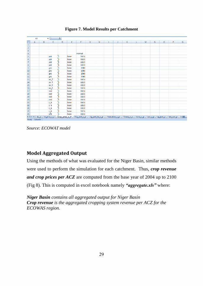
Model Results Once the model input data are completed for the catchment, the model is run

using non-linear programming option CONOPT as a solver. The obtained

results are listed in a notebook namely “Basinname.B.ww_Basin”. This is

illustrated in Figure 7 below where

Bu_p describes crop water consumption per ha;

28

M_price_v_p expresses crop prices;

Tag_prof_v_p defines cropping system total profitability for the whole

catchment;

Ag_prof_v_p defines cropping system profitability per user. Here end users

are trans-boundary countries;

Production_v_p is the cropping system production per ACZ;

Tacre expresses the land allocation per end user;

Acre expresses the land allocation per cropping system technology (rainfall

and irrigated crops) and per end user;

Ben_s_p is the benefit of water end users per nodes;

Ag_ben_p is the agricultural benefit;

Tot_ben_s is the total benefit of water usage by all end users for the whole

catchment.

29

Figure 7. Model Results per Catchment

Source: ECOWAT model

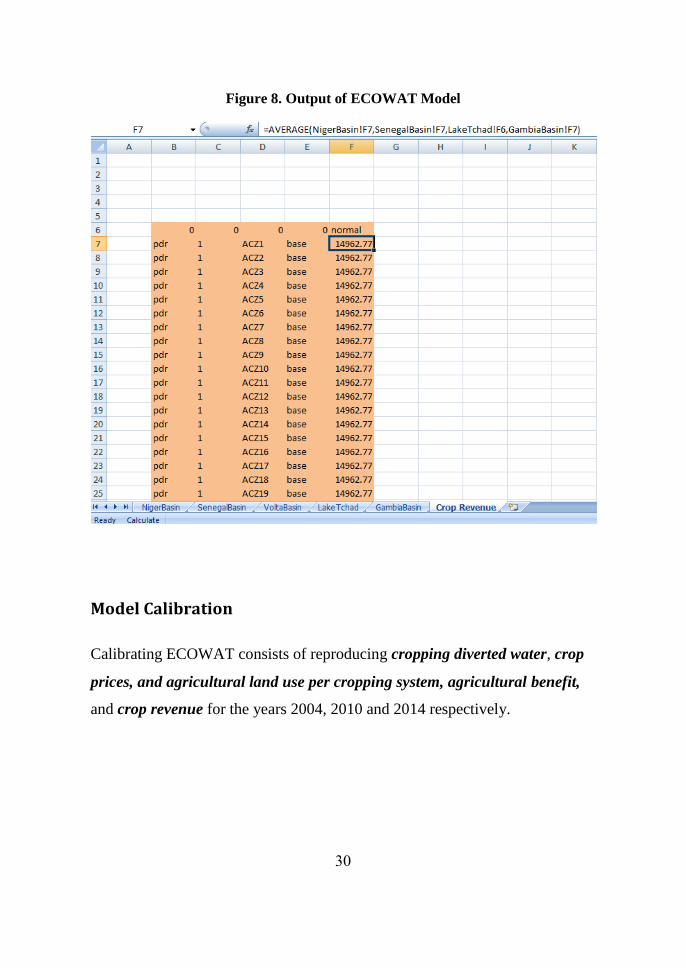
Model Aggregated Output

Using the methods of what was evaluated for the Niger Basin, similar methods

were used to perform the simulation for each catchment. Thus, crop revenue

and crop prices per ACZ are computed from the base year of 2004 up to 2100

(Fig 8). This is computed in excel notebook namely “aggregate.xls” where:

Niger Basin contains all aggregated output for Niger Basin

Crop revenue is the aggregated cropping system revenue per ACZ for the

ECOWAS region.

30

Figure 8. Output of ECOWAT Model

Model Calibration

Calibrating ECOWAT consists of reproducing cropping diverted water, crop

prices, and agricultural land use per cropping system, agricultural benefit,

and crop revenue for the years 2004, 2010 and 2014 respectively.

31

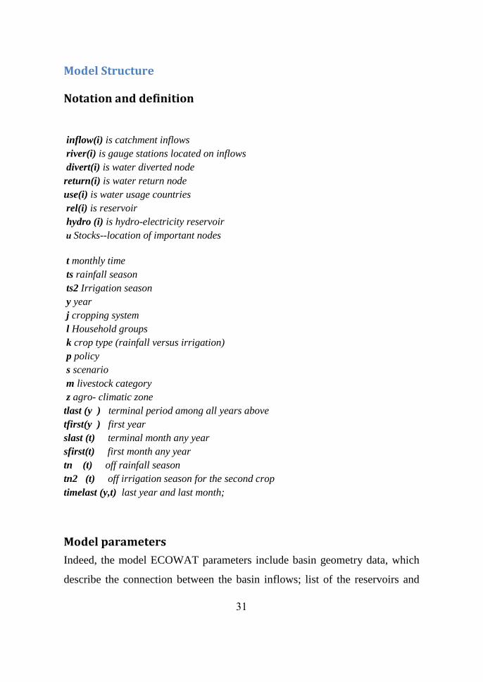
Model Structure

Notation and definition

inflow(i) is catchment inflows

river(i) is gauge stations located on inflows

divert(i) is water diverted node

return(i) is water return node

use(i) is water usage countries

rel(i) is reservoir

hydro (i) is hydro-electricity reservoir

u Stocks--location of important nodes

t monthly time

ts rainfall season

ts2 Irrigation season

y year

j cropping system

l Household groups

k crop type (rainfall versus irrigation)

p policy

s scenario

m livestock category

z agro- climatic zone

tlast (y ) terminal period among all years above

tfirst(y ) first year

slast (t) terminal month any year

sfirst(t) first month any year

tn (t) off rainfall season

tn2 (t) off irrigation season for the second crop

timelast (y,t) last year and last month;

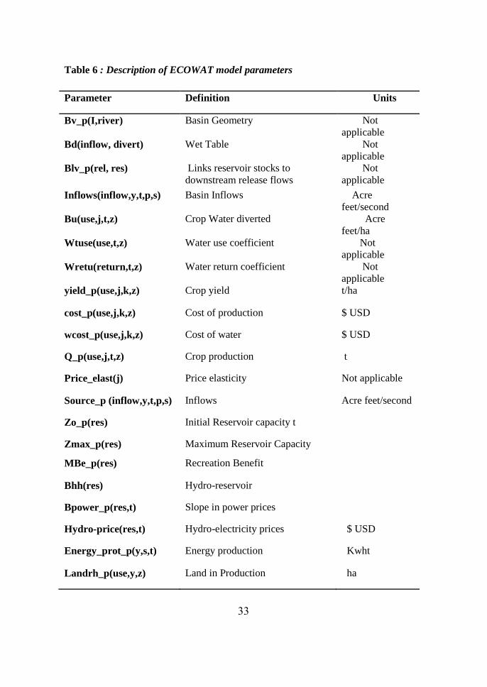
Model parameters

Indeed, the model ECOWAT parameters include basin geometry data, which

describe the connection between the basin inflows; list of the reservoirs and

32

their physical characteristics; base year data of water end users. This includes

diverted water for cropping system, livestock production, energy production

and recreation; their respective water usage efficiency coefficient (Table 7).

33

Table 6 : Description of ECOWAT model parameters

Parameter Definition Units

Bv_p(I,river) Basin Geometry Not

applicable

Bd(inflow, divert) Wet Table Not

applicable

Blv_p(rel, res) Links reservoir stocks to

downstream release flows

Not

applicable

Inflows(inflow,y,t,p,s) Basin Inflows Acre

feet/second

Bu(use,j,t,z) Crop Water diverted Acre

feet/ha

Wtuse(use,t,z) Water use coefficient Not

applicable

Wretu(return,t,z) Water return coefficient Not

applicable

yield_p(use,j,k,z) Crop yield t/ha

cost_p(use,j,k,z) Cost of production $ USD

wcost_p(use,j,k,z) Cost of water $ USD

Q_p(use,j,t,z) Crop production t

Price_elast(j) Price elasticity Not applicable

Source_p (inflow,y,t,p,s) Inflows Acre feet/second

Zo_p(res) Initial Reservoir capacity t

Zmax_p(res) Maximum Reservoir Capacity

MBe_p(res) Recreation Benefit

Bhh(res) Hydro-reservoir

Bpower_p(res,t) Slope in power prices

Hydro-price(res,t) Hydro-electricity prices $ USD

Energy_prot_p(y,s,t) Energy production Kwht

Landrh_p(use,y,z) Land in Production ha

34

Table 7 : Description of ECOWAT model parameters (cont’d)

parameters Definition Units

Mu_use_base_p(I,l,t,z) Household base water

delivery

Acre feet/hh/year

htuse Household water use

efficiency

Not applicable

hrtu Household water use

return coefficient

Not applicable

pop Living population peoples

Hhsize Household size people

P_elasticity_p Urban water demand

elasticity

$ USD/acre feet/hh/year

Mu_price_base base year household

water price

$ USD/hh

AC_uuse0_p base year marginal cost

of supply

$ USD/hh

hhgrowth household population

annual growth rate

Not applicable

mbase_p total livestock population

water demand

Acre feet

mtuse livestock water use

coefficient

Not applicable

mretu livestock water return

coefficient

Not Applicable

mpop livestock monthly base

year population

head

Q_m base year livestock

production

head

price_elast_m price elasticity of

livestock demand

$ USD/head

p_m observed livestock price $ USD

cost_m livestock production cost $ USD

mgrowth growth rate of livestock

population

Not applicable

Model Variables

Following the model objective, which is to optimize water end users’ benefit

for each catchment, model variables are variables describing inter-temporal

water consumption behaviour and profitability of each end user. This included

land use in production, cultivated land per cropping system, reservoir capacity,

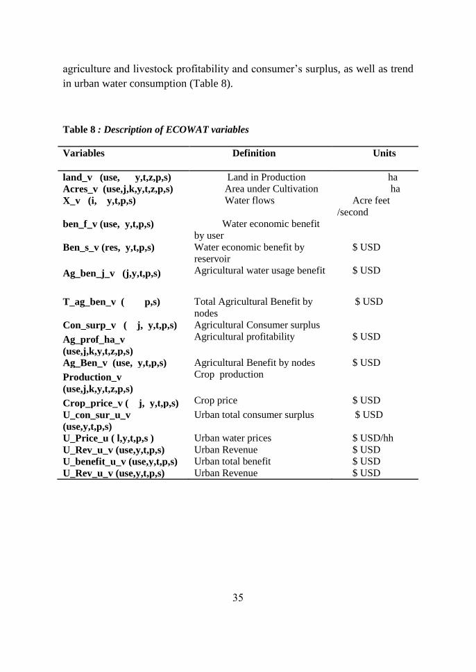
35

agriculture and livestock profitability and consumer’s surplus, as well as trend

in urban water consumption (Table 8).

Table 8 : Description of ECOWAT variables

Variables Definition Units

land_v (use, y,t,z,p,s) Land in Production ha

Acres_v (use,j,k,y,t,z,p,s) Area under Cultivation ha

X_v (i, y,t,p,s) Water flows Acre feet

/second

ben_f_v (use, y,t,p,s) Water economic benefit

by user

Ben_s_v (res, y,t,p,s) Water economic benefit by

reservoir

$ USD

Ag_ben_j_v (j,y,t,p,s) Agricultural water usage benefit $ USD

T_ag_ben_v ( p,s) Total Agricultural Benefit by

nodes

$ USD

Con_surp_v ( j, y,t,p,s) Agricultural Consumer surplus

Ag_prof_ha_v

(use,j,k,y,t,z,p,s)

Agricultural profitability $ USD

Ag_Ben_v (use, y,t,p,s) Agricultural Benefit by nodes $ USD

Production_v

(use,j,k,y,t,z,p,s)

Crop production

Crop_price_v ( j, y,t,p,s) Crop price $ USD

U_con_sur_u_v

(use,y,t,p,s)

Urban total consumer surplus $ USD

U_Price_u ( l,y,t,p,s ) Urban water prices $ USD/hh

U_Rev_u_v (use,y,t,p,s) Urban Revenue $ USD

U_benefit_u_v (use,y,t,p,s) Urban total benefit $ USD

U_Rev_u_v (use,y,t,p,s) Urban Revenue $ USD

36

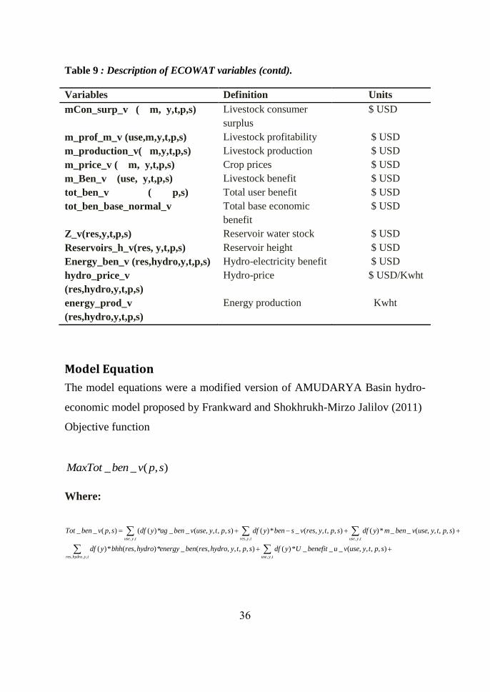
Table 9 : Description of ECOWAT variables (contd).

Variables Definition Units

mCon_surp_v ( m, y,t,p,s) Livestock consumer

surplus

$ USD

m_prof_m_v (use,m,y,t,p,s) Livestock profitability $ USD

m_production_v( m,y,t,p,s) Livestock production $ USD

m_price_v ( m, y,t,p,s) Crop prices $ USD

m_Ben_v (use, y,t,p,s) Livestock benefit $ USD

tot_ben_v ( p,s) Total user benefit $ USD

tot_ben_base_normal_v Total base economic

benefit

$ USD

Z_v(res,y,t,p,s) Reservoir water stock $ USD

Reservoirs_h_v(res, y,t,p,s) Reservoir height $ USD

Energy_ben_v (res,hydro,y,t,p,s) Hydro-electricity benefit $ USD

hydro_price_v

(res,hydro,y,t,p,s)

Hydro-price $ USD/Kwht

energy_prod_v

(res,hydro,y,t,p,s)

Energy production Kwht

Model Equation

The model equations were a modified version of AMUDARYA Basin hydro-

economic model proposed by Frankward and Shokhrukh-Mirzo Jalilov (2011)

Objective function

_ _ ( , )MaxTot ben v p s

Where:

, , , , , ,

, , , , ,

_ _ ( , ) ( ( )* _ _ ( , , , , ) ( )* _ ( , , , , ) ( )* _ _ ( , , , , )

( )* ( , )* _ ( , , , , , ) ( )

use y t res y t use y t

res hydro y t use y t

Tot ben v p s df y ag ben v use y t p s df y ben s v res y t p s df y m ben v use y t p s

df y bhh res hydro energy ben res hydro y t p s df y

* _ _ _ ( , , , , )U benefit u v use y t p s

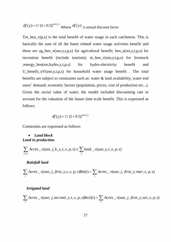
37

( )( ) 1/ (1 0.5)ord ydf y Where ( )df y is annual discount factor

Tot_ben_v(p,s) is the total benefit of water usage in each catchment. This is

basically the sum of all the basin related water usage activities benefit and

these are ag_ben_v(use,y,t,p,s) for agricultural benefit; ben_s(res,y,t,p,s) for

recreation benefit (include tourism); m_ben_v(use,y,t,p,s) for livestock

;energy_ben(res,hydro,y,t,p,s) for hydro-electricity benefit and

U_benefit_uV(use,y,t,p,s) for household water usage benefit . The total

benefits are subject to constraints such as: water & land availability, water end

users’ demand, economic factors (population, prices, cost of production etc...).

Given the social value of water, the model included discounting rate to

account for the valuation of the future time scale benefit. This is expressed as

follows.

Constraints are expressed as follows

Land block

Land in production

, ,

_ ( , , , , , , , ) _ ( , , , , , )j k z z

Acres v use j k y t z p s land v use y t z p s

Rainfall land

_ ( , , , , , , , )$ ( ) _ ( , , , , , , , )z z

Acres v use j first y t z p s ts t Acres v use j first y mar z p s

Irrigated land

_ ( , ,sec , , , , , )$ 2( ) _ ( , , , , , , , )z z

Acres v use j ond y t z p s ts t Acres v use j first y oct z p s

( )( ) 1/ (1 0.5)ord ydf y

38

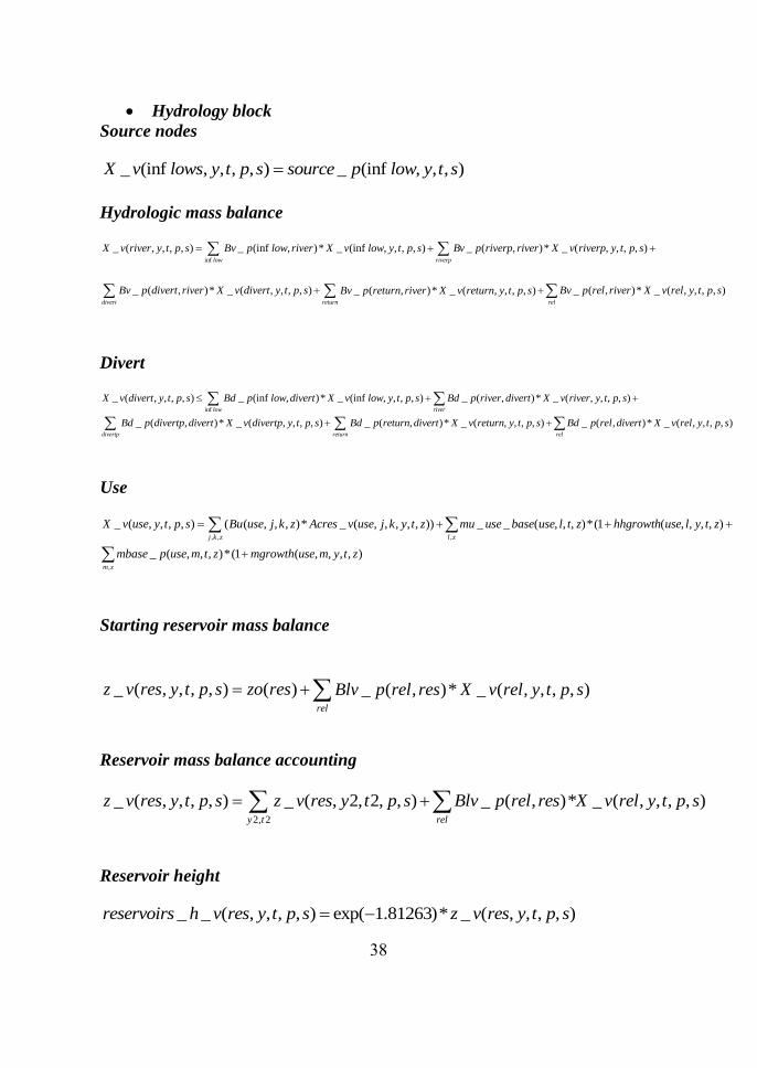
Hydrology block

Source nodes

_ (inf , , , , ) _ (inf , , , )X v lows y t p s source p low y t s

Hydrologic mass balance

inf

_ ( , , , , ) _ (inf , )* _ (inf , , , , ) _ ( , )* _ ( , , , , )

_ ( , )* _ ( , , , , ) _ ( , )* _ ( , , , , )

low riverp

diver return

X v river y t p s Bv p low river X v low y t p s Bv p riverp river X v riverp y t p s

Bv p divert river X v divert y t p s Bv p return river X v return y t p s

_ ( , )* _ ( , , , , )t rel

Bv p rel river X v rel y t p s

Divert

inf

_ ( , , , , ) _ (inf , )* _ (inf , , , , ) _ ( , )* _ ( , , , , )

_ ( , )* _ ( , , , , ) _ ( , )* _ ( , , , , ) _ (

low river

X v divert y t p s Bd p low divert X v low y t p s Bd p river divert X v river y t p s

Bd p divertp divert X v divertp y t p s Bd p return divert X v return y t p s Bd p re

, )* _ ( , , , , )divertp return rel

l divert X v rel y t p s

Use

, , ,

,

_ ( , , , , ) ( ( , , , )* _ ( , , , , , )) _ _ ( , , , )*(1 ( , , , , )

_ ( , , , )*(1 ( , , , , )

j k z l z

m z

X v use y t p s Bu use j k z Acres v use j k y t z mu use base use l t z hhgrowth use l y t z

mbase p use m t z mgrowth use m y t z

Starting reservoir mass balance

_ ( , , , , ) ( ) _ ( , )* _ ( , , , , )rel

z v res y t p s zo res Blv p rel res X v rel y t p s

Reservoir mass balance accounting

2, 2

_ ( , , , , ) _ ( , 2, 2, , ) _ ( , )* _ ( , , , , )y t rel

z v res y t p s z v res y t p s Blv p rel res X v rel y t p s

Reservoir height

_ _ ( , , , , ) exp( 1.81263)* _ ( , , , , )reservoirs h v res y t p s z v res y t p s

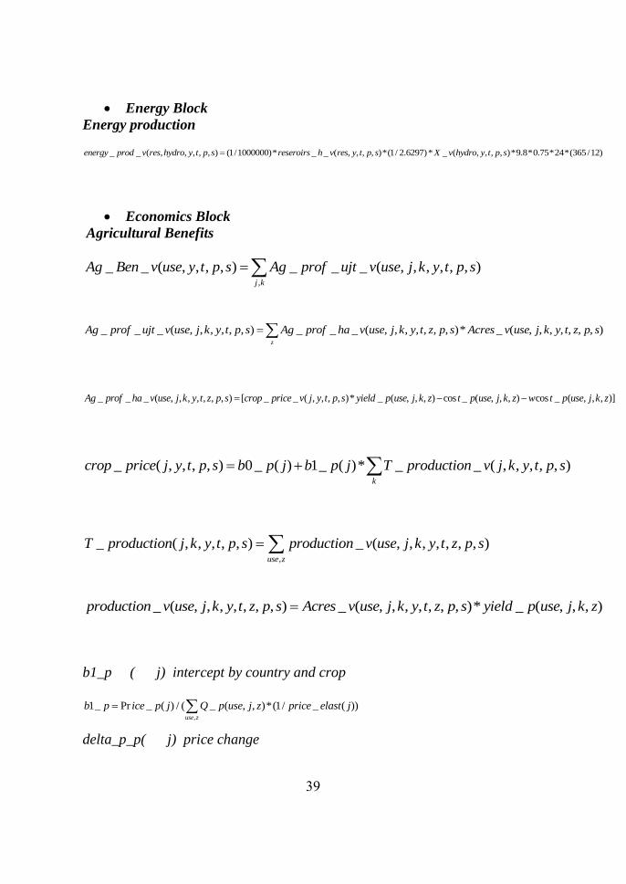
39

Energy Block

Energy production

_ _ ( , , , , , ) (1/1000000)* _ _ ( , , , , )*(1/ 2.6297)* _ ( , , , , )*9.8*0.75*24*(365 /12)energy prod v res hydro y t p s reseroirs h v res y t p s X v hydro y t p s

Economics Block

Agricultural Benefits

,

_ _ ( , , , , ) _ _ _ ( , , , , , , )j k

Ag Ben v use y t p s Ag prof ujt v use j k y t p s

_ _ _ ( , , , , , , ) _ _ _ ( , , , , , , , )* _ ( , , , , , , , )z

Ag prof ujt v use j k y t p s Ag prof ha v use j k y t z p s Acres v use j k y t z p s

_ _ _ ( , , , , , , , ) [ _ _ ( , , , , )* _ ( , , , ) cos _ ( , , , ) cos _ ( , , , )]Ag prof ha v use j k y t z p s crop price v j y t p s yield p use j k z t p use j k z w t p use j k z

_ ( , , , , ) 0 _ ( ) 1_ ( )* _ _ ( , , , , , )k

crop price j y t p s b p j b p j T production v j k y t p s

,

_ ( , , , , , ) _ ( , , , , , , , )use z

T production j k y t p s production v use j k y t z p s

_ ( , , , , , , , ) _ ( , , , , , , , )* _ ( , , , )production v use j k y t z p s Acres v use j k y t z p s yield p use j k z

b1_p ( j) intercept by country and crop

delta_p_p( j) price change

,

1_ Pr _ ( ) / ( _ ( , , )*(1/ _ ( ))use z

b p ice p j Q p use j z price elast j

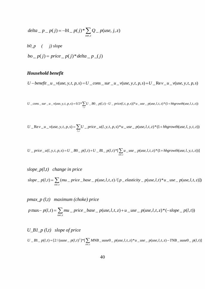
40

,

_ _ ( ) 1_ ( )* _ ( , , )use z

delta p p j b p j Q p use j z

b0_p ( j) slope

_ ( ) _ ( )* _ _( )bo p j price p j delta p j

Household benefit

_ _ ( , , , , ) _ _ _ _ ( , , , , ) _ Re _ _ ( , , , , )U benefit u v use y t p s U cons sur u v use y t p s U v u v use y t p s

,

_ _ _ _ ( , , , , ) 0.5* _ 0 _ ( , ) _ ( , , , )]* _ _ ( , , , )*(1 ( , , , ))l z

U cons sur u v use y t p s U B p l t U price l t p s u use p use l t z hhgrowth use l t z

,

_ Re _ _ ( , , , , ) _ _ ( , , , , )* _ _ ( , , , )*(1 ( , , , , ))l z

U v u v use y t p s U price u l y t p s u use p use l t z hhgrowth use l y t z

,

_ _ ( , , , , ) _ 0 _ ( , ) _ 1_ ( , )*[ _ _ ( , , , )*(1 ( , , , , ))]use z

U price u l y t p s U B p l t U B p l t u use p use l t z hhgrowth use l y t z

slope_p(l,t) change in price

,

_ ( , ) ( _ _ _ ( , , , ) / [ _ _ ( , , )* _ _ ( , , , )])use z

slope p l t mu price base p use l t z p elasticity p use l t u use p use l t z

pmax_p (l,t) maximum (choke) price

,

max ( , ) _ _ _ ( , , , ) _ _ ( , , , )*( _ ( , ))use z

p p l t mu price base p use l t z u use p use l t z slope p l t

U_B1_p (l,t) slope of price

2

,

_ 1_ ( , ) [2 / ( _ ( , ) ]*[ _ 0 _ ( , , , )* _ _ ( , , , ) _ 0 _ ( , )]use z

U B p l t uuse p l t MNB uuse p use l t z u use p use l t z TNB uuse p l t

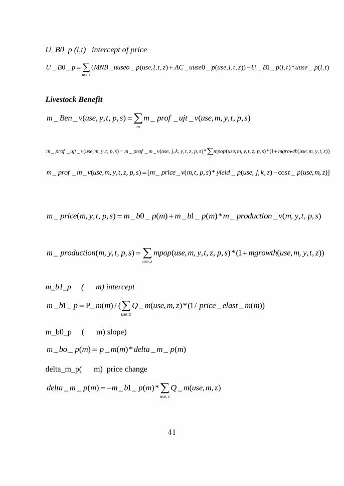
41

U_B0_p (l,t) intercept of price

,

_ 0 _ ( _ _ ( , , , ) _ 0 _ ( , , , )) _ 1_ ( , )* _ ( , )use z

U B p MNB uuseo p use l t z AC uuse p use l t z U B p l t uuse p l t

Livestock Benefit

_ _ ( , , , , ) _ _ _ ( , , , , , )m

m Ben v use y t p s m prof ujt v use m y t p s

_ _ _ ( , , , , , ) _ _ _ ( , , , , , , , )* ( , , , , , , )*(1 ( , , , , ))z

m prof ujt v use m y t p s m prof m v use j k y t z p s mpop use m y t z p s mgrowth use m y t z

_ _ _ ( , , , , , , ) [ _ _ ( , , , )* _ ( , , , ) cos _ ( , , )]m prof m v use m y t z p s m price v m t p s yield p use j k z t p use m z

_ ( , , , , ) _ 0_ ( ) _ 1_ ( )* _ _ ( , , , , )m price m y t p s m b p m m b p m m production v m y t p s

,

_ ( , , , , ) ( , , , , , , )*(1 ( , , , , ))use z

m production m y t p s mpop use m y t z p s mgrowth use m y t z

m_b1_p ( m) intercept

,

_ 1_ P_ ( ) / ( _ ( , , )*(1/ _ _ ( ))use z

m b p m m Q m use m z price elast m m

m_b0_p ( m) slope)

_ _ ( ) _ ( )* _ _ ( )m bo p m p m m delta m p m

delta_m_p( m) price change

,

_ _ ( ) _ 1_ ( )* _ ( , , )use z

delta m p m m b p m Q m use m z

42

Hydro-electricity Benefit

_ _ ( , , , , , ) _ _ ( , , , , , )* _ ( , )energy ben v res hydro y t p s energy prod v res hydro y t p s hydro price res t

Recreation Benefit

_ _ ( , , , , ) _ ( )* _ ( , , , , )Ben s e res y t p s MBe p res z v res y t p s

43

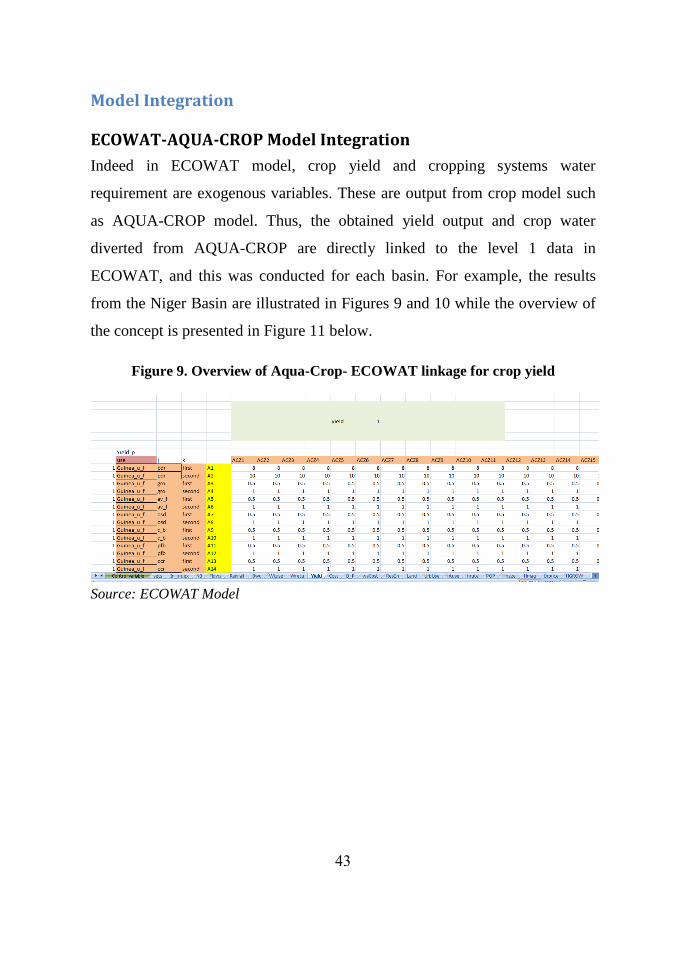
Model Integration

ECOWAT-AQUA-CROP Model Integration

Indeed in ECOWAT model, crop yield and cropping systems water

requirement are exogenous variables. These are output from crop model such

as AQUA-CROP model. Thus, the obtained yield output and crop water

diverted from AQUA-CROP are directly linked to the level 1 data in

ECOWAT, and this was conducted for each basin. For example, the results

from the Niger Basin are illustrated in Figures 9 and 10 while the overview of

the concept is presented in Figure 11 below.

Figure 9. Overview of Aqua-Crop- ECOWAT linkage for crop yield

Source: ECOWAT Model

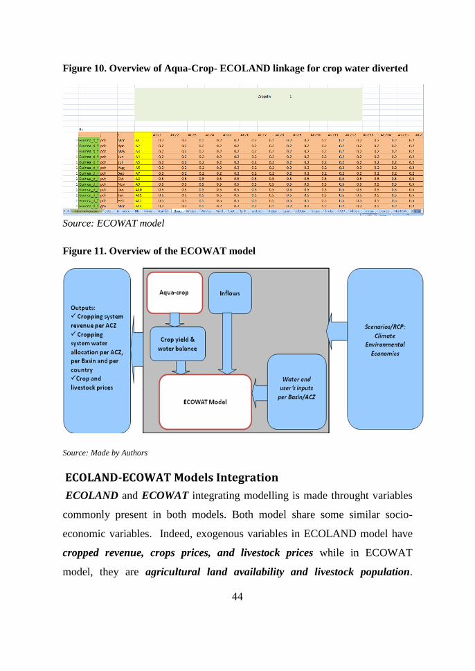
44

Figure 10. Overview of Aqua-Crop- ECOLAND linkage for crop water diverted

Source: ECOWAT model

Figure 11. Overview of the ECOWAT model

Source: Made by Authors

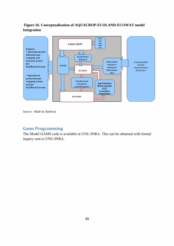
ECOLAND-ECOWAT Models Integration

ECOLAND and ECOWAT integrating modelling is made throught variables

commonly present in both models. Both model share some similar socio-

economic variables. Indeed, exogenous variables in ECOLAND model have

cropped revenue, crops prices, and livestock prices while in ECOWAT

model, they are agricultural land availability and livestock population.

45

However, agricultural land availability and livestock population are the

output of ECOLAND, while revenue, crop prices, and livestock prices are the

output of ECOWAT. Thus, the integration consists of linking ECOLAND

selected output value as input in ECOWAT at first scenario level and vice

versa. This is illustrated in Figures 12-15 and the conceptualized framework is

presented in Figure16 below.

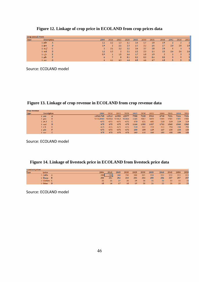
46

Figure 12. Linkage of crop price in ECOLAND from crop prices data

Source: ECOLAND model

Figure 13. Linkage of crop revenue in ECOLAND from crop revenue data

Source: ECOLAND model

Figure 14. Linkage of livestock price in ECOLAND from livestock price data

Source: ECOLAND model

47

Source: ECOWAT Model

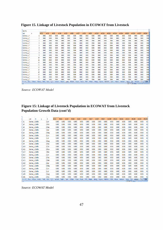
Figure 15: Linkage of Livestock Population in ECOWAT from Livestock

Population Growth Data (cont’d)

Source: ECOWAT Model

Figure 15. Linkage of Livestock Population in ECOWAT from Livestock

Population growth Data

48

Figure 16. Conceptualization of AQUACROP-ECOLAND-ECOWAT model

Integration

Source: Made by Authors)

Gams Programming The Model GAMS code is available at UNU-INRA. This can be obtained with formal

inquiry sent to UNU-INRA.

49

ECOTRADE -Trade Model

Introduction The ECOWAS region trade model so-called ECOTRAD was developed using

the MIRAGE model (Yvan and Hugo, 2007). It is a sequence dynamic

recursive CGE model. The model accommodates the GTAP8 Africa database

to the MIRAGE model given the difference of nomenclature. In ECOTRAD,

using gtapagg the world is disaggregated into 19 regions. These includes nine

ECOWAS countries namely Benin, Burkina-Faso, Ivory-coast, Ghana,

Guinea, Nigeria, Senegal, Togo and rest of ECOWAS countries; one region

for the Rest of Sub-Sahara Africa; one region for Middle East and Northern

Africa(MENA);; one region each for respectively Oceania, East -Asia , South-

East Asia, South Asia, North America , Latin America , Europe ,and the Rest

of the World.

In addition, the sectors were disaggregated into 31 economics sectors of which

12 agricultural sectors, 12 industrial sectors and seven (7) services sectors. For

the purpose of food security analysis, food crops includes agricultural crops

and process food. .

The model has been adjusted to include the ECOWAS Common External

Tariff policy (CET) for the Business as Usual (BAU) scenarios. It aims to

assess the impact of occurring changes in respectively cropping land

allocation, cropping water allocation and in domestic supply of agricultural

commodities on agricultural trade flow and national food security. It is an

economy-wide impact assessment and provides useful output for decision-

making on how to improve trade and food security in ECOWAS countries.

50

Model Overview

Description

The model is made of 3 main folders respectively Data; Scenarios and

Results and 11 main Gams files respectively SET.gms; Data.gms; Calib.gms;

MDS_INIT.gms; MDS.gm; Option.gms; REF_Init.gms; REF.gms;

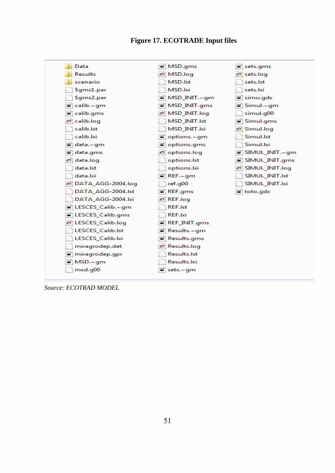
Simul_INIT.gms; Simul.gms and Results.gms. This is illustrated in Figure 17

below where:

Data: Contain the model input data;

Scenarios: contain the model scenarios data;

Results: contain the model output after simulation;

SET.gms: define the model notation information

Data.gms: run for adjustments, aggregation of model input data

Calib.gms: run for model data calibration

MDS_INIT.gms: initialization of model variable and parameters

MDS.gm: BAU computation

Option.gms: Model option definition such as time horizon

REF_Init.gms: Reference scenario definition

REF.gms: reference scenario computation

Simul_INIT.gms: simulation of BAU

Simul.gms: Model simulation

Results.gms:

51

Source: ECOTRAD MODEL

Figure 17. ECOTRADE Input files

52

Model Data

The model data basically includes base year data DATA1_AGG-2004.gdx

computed using basedata2004.gdx data. However, basedata2004.gdx is built

using GAgg8 platform. In doing so, the step of computing basedata2004.gdx

using GAgg8 is as follows:

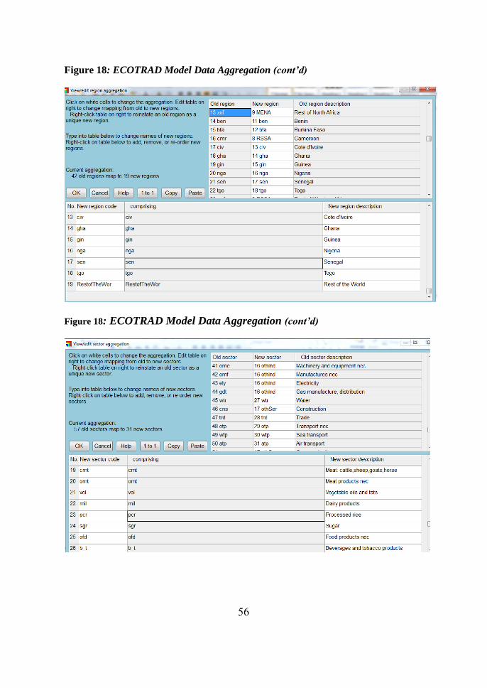
First, install GAgg81Afry04 on your C: / drive.

Open GTAPAgg, after go to View/Change regional aggregation. From this

section, there are 42 regions which are aggregated into 19 regions. These

include Rep. of Benin, Burkina-Faso, Ivory-coast, Ghana, Guinea, Nigeria,

Senegal, Togo and the rest of ECOWAS countries for ECOWAS region. One

region for the Rest of Sub-Sahara Africa (Botswana, Cameroun, Ethiopia,

Kenya, Madagascar, Mozambique, Mauritius, Malawi, Namibia, Rwanda

,Tanzania, Uganda, South Africa, Zambia, Zimbabwe, Rest of Eastern Africa,

Rest of Central Africa, Rest of Southern Africa) ; MENA( Middle Est-North

Africa); Oceania; East -Asia ; South-East Asia; South Asia; North America ;

Latin America ; Europe -27 ( 27 countries in Europe) and the Rest of the Word

( the Rest of World and the Rest of Europe).

Once this is done, the new aggregation is saved using save aggregation

scheme to file.

The similarity method is used for sectoral aggregation using View/Changes

sectoral aggregation. Existing 57 old sectoral aggregations are aggregated

into sectoral 31 sectors. This include 12 agricultural sectors namely paddy

rice; wheat; cereal; vegetable –fruits-nuts; oil seeds; sugarcane-sugarbeet ;

fibers and other indigenous crops ; livestock; animal product nec ; forestry and

fishery, 12 industrial sector’s mainly meat; other meat products; raw milk;

Processed food; Vegetable oil; Dairy products ; Processed rice; Sugar; other

food products ; beverage and tabocco; extracted oil and other industries; seven

53

(7) service sectors mainly water; electricity; public

administration/defense/education/health/defense and other services.

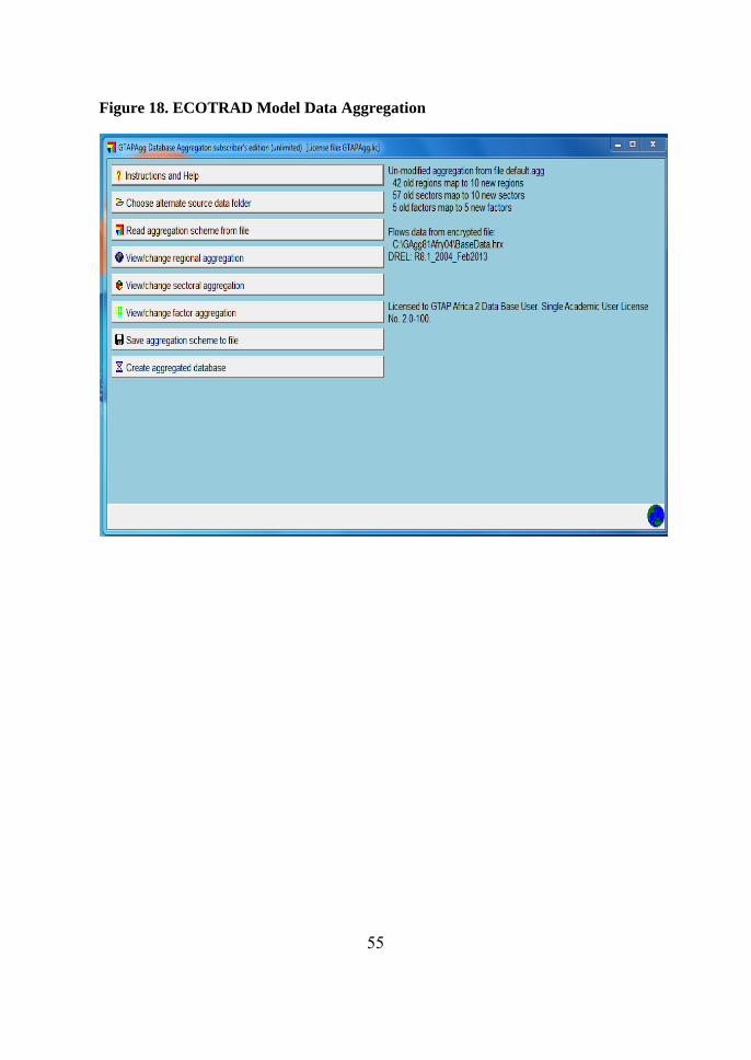
The aggregated input is then created by running Create aggregated database

(Figure 18). In the generated files two important files are extracted and these

are: BaseData.har and Default.prm respectively which are the base year data

and the parameters database. Indeed, GAMS cannot read HAR files directly.

However, it is easy to convert them to GDX files. Create a new project in your

GTAP8 working directory, where the HAR files are stored. Then create a new

GAMS file, which may be named HAR2GDX.gms and which contains only

two lines:

54

$CALL har2gdx basedata2004.har basedata2004.gdx

$CALL har2gdx parameters2004.har parameters2004.gdx

Other input data are ELAST_PAR.gdx, VAL_PAR.gdx, prices elasticity and

income elasticity; and DATA.gdx which contains exogenous parameters such

as populations and GDP growth.

Thus, using DATA_AGG-2004.gms, the model base year on 2004 input data is

generated and this is called DATA1_AGG-2004.gdx.This includes sets and

parameters listed below. Sets are:

Agr: all agricultural commodities definition;

AgrTot: All agricultural sectors include food sector;

ENDW_COMM: all endowment commodities mainly land, capital, natural

resources, and skill and unskilled labour;

GTAP_I: GTAP sectors;

GTAP_R: GTAP regions;

Icp: perfect competition commodities;

L_1: Skill labour;

MAP_I: sectoral mapping between GTAP and ECOTRAD sector;

MAP_R: Region mapping between GTAP and ECOTRAD region;

Nord: Developed regions;

Prod_comm: produced commodities;

Reg: GTAP regions;

Scareland: Scarcity land regions;

Simple: import demand tree;

TRAD_COMM: trade commodities;

Transporation: transport sectors;and

Unchanged: GTAP tariffs,

55

Figure 18. ECOTRAD Model Data Aggregation

56

Figure 18: ECOTRAD Model Data Aggregation (cont’d)

Figure 18: ECOTRAD Model Data Aggregation (cont’d)

57

Model Output

These are variables for accessing the impact of climate change on trade flows

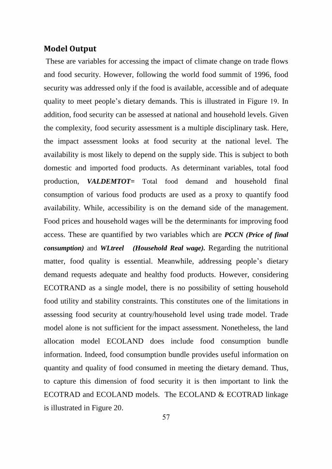
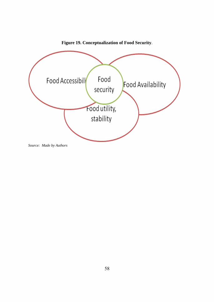
and food security. However, following the world food summit of 1996, food

security was addressed only if the food is available, accessible and of adequate

quality to meet people’s dietary demands. This is illustrated in Figure 19. In

addition, food security can be assessed at national and household levels. Given

the complexity, food security assessment is a multiple disciplinary task. Here,

the impact assessment looks at food security at the national level. The

availability is most likely to depend on the supply side. This is subject to both

domestic and imported food products. As determinant variables, total food

production, VALDEMTOT= Total food demand and household final

consumption of various food products are used as a proxy to quantify food

availability. While, accessibility is on the demand side of the management.

Food prices and household wages will be the determinants for improving food

access. These are quantified by two variables which are PCCN (Price of final

consumption) and WLtreel (Household Real wage). Regarding the nutritional

matter, food quality is essential. Meanwhile, addressing people’s dietary

demand requests adequate and healthy food products. However, considering

ECOTRAND as a single model, there is no possibility of setting household

food utility and stability constraints. This constitutes one of the limitations in

assessing food security at country/household level using trade model. Trade

model alone is not sufficient for the impact assessment. Nonetheless, the land

allocation model ECOLAND does include food consumption bundle

information. Indeed, food consumption bundle provides useful information on

quantity and quality of food consumed in meeting the dietary demand. Thus,

to capture this dimension of food security it is then important to link the

ECOTRAD and ECOLAND models. The ECOLAND & ECOTRAD linkage

is illustrated in Figure 20.

58

Figure 19. Conceptualization of Food Security.

Source: Made by Authors

59

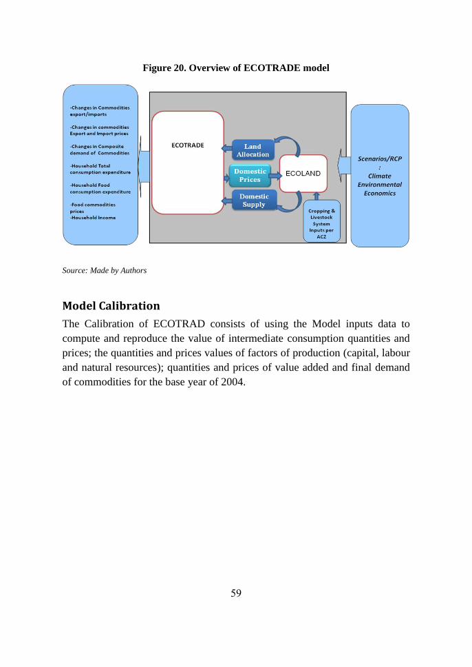
Figure 20. Overview of ECOTRADE model

Source: Made by Authors

Model Calibration

The Calibration of ECOTRAD consists of using the Model inputs data to

compute and reproduce the value of intermediate consumption quantities and

prices; the quantities and prices values of factors of production (capital, labour

and natural resources); quantities and prices of value added and final demand

of commodities for the base year of 2004.

60

Model Structure

Notation and Definition

Region:

This includes Benin.(ben), Burkina.(bfa), Ivory.(civ), Ghana.(gha),

Guinea.(gin), Nigeria

(nga),Senegal.(sen),Togo.(tgo),RWA.(xwf),EASIA.(EAsia),SEASIA.(SEAsia)

,SASIA.(SoutAsia), NAmerica. (North America), LAmerica. (Latin America),

EUROPE. (EU27), MENA. (MiddleEast,egy,mar,tun,xnf), RSSA.(bwa,cmr,

eth,ken, mdg, moz, mus, mwi, nam,rwa,tza, uga, zaf, zmb,

zwe,xec,xsc,xcf,xac), OCEANIA. (Oceania), RoW. (Rest of TheWor

,RestEurope).

Time: from year 2004 to 2100

J is used for definition of sectors. These are mainly agricultural, industries,

services and administrative sectors listed by pdr(paddy rice), wht(wheat),

gro(cereal),v_f(vegetable), osd(oil seed), c_b(sugarcane/sugarbeet), pfb(plant

& fiber); ocr(crop nec); ctl(cattle,sheep,goat); oap(animal products), rmk(raw

milk), wol, frs(fruits), fsh(fish), cmt(meat products), omt(meat products nec);

vol(vegetable); mil(dairy products), pcr(processed rice); sgr(sugar); ofd(food

products nec);b_t(beverage & tabacco);ely(electricity); wtr(water); oil(oil);

osg(public administration/defense/education/health) ; othInd(coal,gas,textile,

wearing apparel, leather, woods, paper& publishing, petroleum,chemical,

rubber, plastic, mineral, ferrous, metal, motor& vehicule, transport,mineral);

othSer( eletronic, machinery and equipment, manifacture, gas

manifacture,construction, trade, transport nec, sea transport, air transport,

communication, financial services, insurance ,business services nec,

recreations & other services, dwellings)

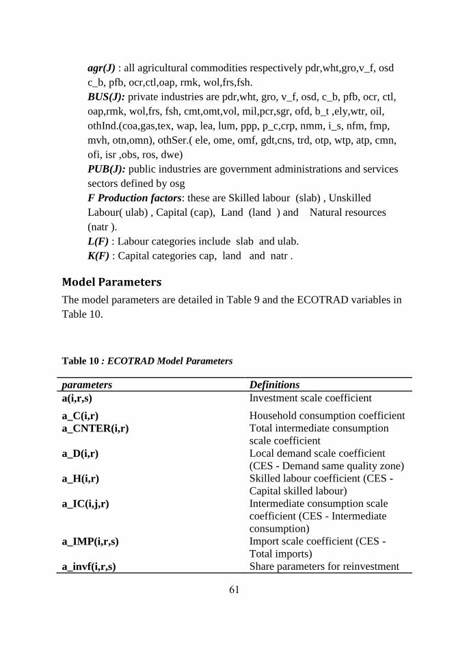
61

agr(J) : all agricultural commodities respectively pdr,wht,gro,v_f, osd

c_b, pfb, ocr,ctl,oap, rmk, wol,frs,fsh.

BUS(J): private industries are pdr,wht, gro, v_f, osd, c_b, pfb, ocr, ctl,

oap,rmk, wol,frs, fsh, cmt,omt,vol, mil,pcr,sgr, ofd, b_t ,ely,wtr, oil,

othInd.(coa,gas,tex, wap, lea, lum, ppp, p_c,crp, nmm, i_s, nfm, fmp,

mvh, otn,omn), othSer.( ele, ome, omf, gdt,cns, trd, otp, wtp, atp, cmn,

ofi, isr ,obs, ros, dwe)

PUB(J): public industries are government administrations and services

sectors defined by osg

F Production factors: these are Skilled labour (slab) , Unskilled

Labour( ulab) , Capital (cap), Land (land ) and Natural resources

(natr ).

L(F) : Labour categories include slab and ulab.

K(F) : Capital categories cap, land and natr .

Model Parameters

The model parameters are detailed in Table 9 and the ECOTRAD variables in

Table 10.

Table 10 : ECOTRAD Model Parameters

parameters Definitions

a(i,r,s) Investment scale coefficient

a_C(i,r) Household consumption coefficient

a_CNTER(i,r) Total intermediate consumption

scale coefficient

a_D(i,r) Local demand scale coefficient

(CES - Demand same quality zone)

a_H(i,r) Skilled labour coefficient (CES -

Capital skilled labour)

a_IC(i,j,r) Intermediate consumption scale

coefficient (CES - Intermediate

consumption)

a_IMP(i,r,s) Import scale coefficient (CES -

Total imports)

a_invf(i,r,s) Share parameters for reinvestment

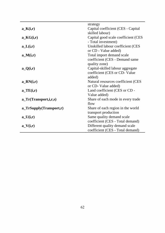
62

strategy

a_K(i,r) Capital coefficient (CES - Capital

skilled labour)

a_KG(i,r) Capital good scale coefficient (CES

- Total investment)

a_L(i,r) Unskilled labour coefficient (CES

or CD - Value added)

a_M(i,r) Total import demand scale

coefficient (CES - Demand same

quality zone)

a_Q(i,r) Capital-skilled labour aggregate

coefficient (CES or CD- Value

added)

a_RN(i,r) Natural resources coefficient (CES

or CD- Value added)

a_TE(i,r) Land coefficient (CES or CD -

Value added)

a_Tr(Transport,i,r,s) Share of each mode in every trade

flow

a_TrSupply(Transport,r) Share of each region in the world

transport production

a_U(i,r) Same quality demand scale

coefficient (CES - Total demand)

a_V(i,r) Different quality demand scale

coefficient (CES - Total demand)

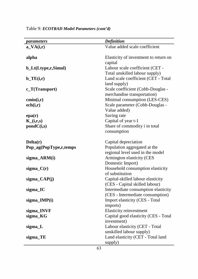
63

Table 9: ECOTRAD Model Parameters (cont’d)

parameters Definition

a_VA(i,r) Value added scale coefficient

alpha Elasticity of investment to return on

capital

b_Lt(Ltype,r,Simul) Labour scale coefficient (CET -

Total unskilled labour supply)

b_TE(i,r) Land scale coefficient (CET - Total

land supply)

c_T(Transport) Scale coefficient (Cobb-Douglas -

merchandise transportation)

cmin(i,r) Minimal consumption (LES-CES)

ech(i,r) Scale parameter (Cobb-Douglas -

Value added)

epa(r) Saving rate

K_(i,r,s) Capital of year t-1

pondC(i,s) Share of commodity i in total

consumption

Delta(r) Capital depreciation

Pop_ag(PopType,r,temps Population aggregated at the

regional level used in the model

sigma_ARM(i) Armington elasticity (CES

Domestic Import)

sigma_C(r) Household consumption elasticity

of substitution

sigma_CAP(j) Capital-skilled labour elasticity

(CES - Capital skilled labour)

sigma_IC Intermediate consumption elasticity

(CES - Intermediate consumption)

sigma_IMP(i) Import elasticity (CES - Total

imports)

sigma_INVF Elasticity reinvestment

sigma_KG Capital good elasticity (CES - Total

investment)

sigma_L Labour elasticity (CET - Total

unskilled labour supply)

sigma_TE Land elasticity (CET - Total land

supply)

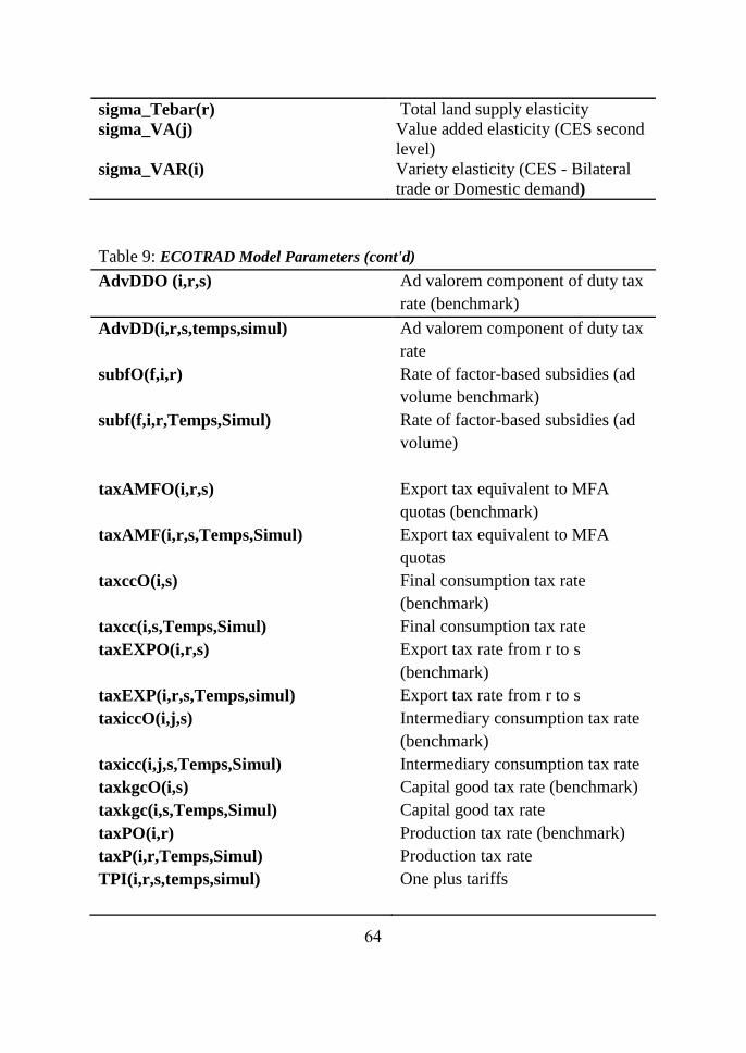
64

sigma_Tebar(r) Total land supply elasticity

sigma_VA(j) Value added elasticity (CES second

level)

sigma_VAR(i) Variety elasticity (CES - Bilateral

trade or Domestic demand)

Table 9: ECOTRAD Model Parameters (cont'd)

AdvDDO (i,r,s) Ad valorem component of duty tax

rate (benchmark)

AdvDD(i,r,s,temps,simul) Ad valorem component of duty tax

rate

subfO(f,i,r) Rate of factor-based subsidies (ad

volume benchmark)

subf(f,i,r,Temps,Simul) Rate of factor-based subsidies (ad

volume)

taxAMFO(i,r,s) Export tax equivalent to MFA

quotas (benchmark)

taxAMF(i,r,s,Temps,Simul) Export tax equivalent to MFA

quotas

taxccO(i,s) Final consumption tax rate

(benchmark)

taxcc(i,s,Temps,Simul) Final consumption tax rate

taxEXPO(i,r,s) Export tax rate from r to s

(benchmark)

taxEXP(i,r,s,Temps,simul) Export tax rate from r to s

taxiccO(i,j,s) Intermediary consumption tax rate

(benchmark)

taxicc(i,j,s,Temps,Simul) Intermediary consumption tax rate

taxkgcO(i,s) Capital good tax rate (benchmark)

taxkgc(i,s,Temps,Simul) Capital good tax rate

taxPO(i,r) Production tax rate (benchmark)

taxP(i,r,Temps,Simul) Production tax rate

TPI(i,r,s,temps,simul) One plus tariffs

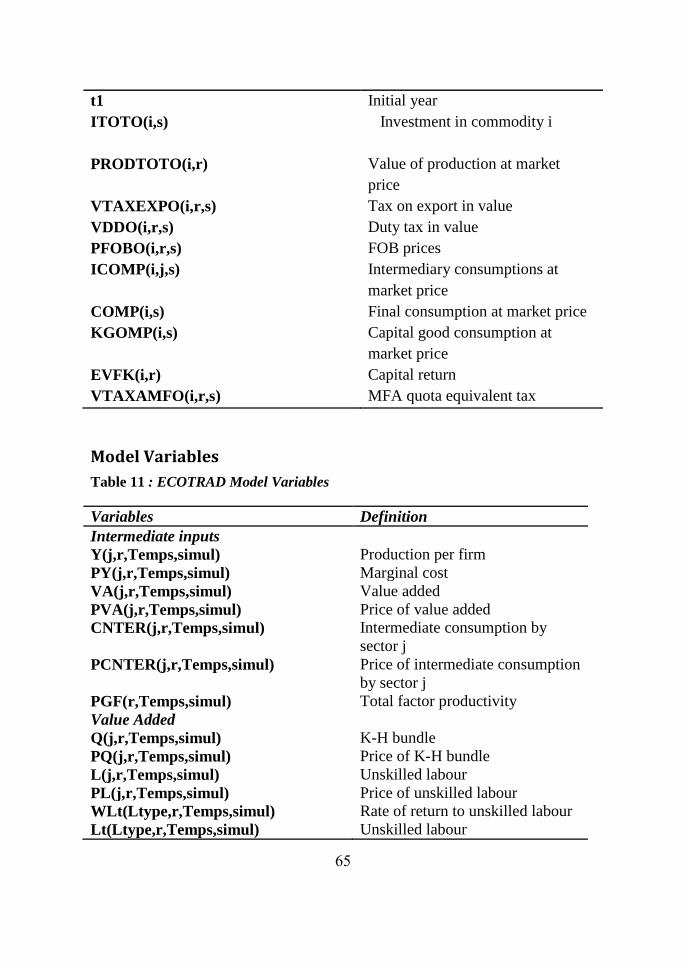
65

t1 Initial year

ITOTO(i,s) Investment in commodity i

PRODTOTO(i,r) Value of production at market

price

VTAXEXPO(i,r,s) Tax on export in value

VDDO(i,r,s) Duty tax in value

PFOBO(i,r,s) FOB prices

ICOMP(i,j,s) Intermediary consumptions at

market price

COMP(i,s) Final consumption at market price

KGOMP(i,s) Capital good consumption at

market price

EVFK(i,r) Capital return

VTAXAMFO(i,r,s) MFA quota equivalent tax

Model Variables

Table 11 : ECOTRAD Model Variables

Variables Definition

Intermediate inputs

Y(j,r,Temps,simul) Production per firm

PY(j,r,Temps,simul) Marginal cost

VA(j,r,Temps,simul) Value added

PVA(j,r,Temps,simul) Price of value added

CNTER(j,r,Temps,simul) Intermediate consumption by

sector j

PCNTER(j,r,Temps,simul) Price of intermediate consumption

by sector j

PGF(r,Temps,simul) Total factor productivity

Value Added

Q(j,r,Temps,simul) K-H bundle

PQ(j,r,Temps,simul) Price of K-H bundle

L(j,r,Temps,simul) Unskilled labour

PL(j,r,Temps,simul) Price of unskilled labour

WLt(Ltype,r,Temps,simul) Rate of return to unskilled labour

Lt(Ltype,r,Temps,simul) Unskilled labour

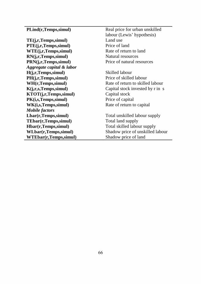
66

PLind(r,Temps,simul) Real price for urban unskilled

labour (Lewis’ hypothesis)

TE(j,r,Temps,simul) Land use

PTE(j,r,Temps,simul) Price of land

WTE(j,r,Temps,simul) Rate of return to land

RN(j,r,Temps,simul) Natural resources

PRN(j,r,Temps,simul) Price of natural resources

Aggregate capital & labor

H(j,r,Temps,simul) Skilled labour

PH(j,r,Temps,simul) Price of skilled labour

WH(r,Temps,simul) Rate of return to skilled labour

K(j,r,s,Temps,simul) Capital stock invested by r in s

KTOT(j,r,Temps,simul) Capital stock

PK(i,s,Temps,simul) Price of capital

WK(i,s,Temps,simul) Rate of return to capital

Mobile factors

Lbar(r,Temps,simul) Total unskilled labour supply

TEbar(r,Temps,simul) Total land supply

Hbar(r,Temps,simul) Total skilled labour supply

WLbar(r,Temps,simul) Shadow price of unskilled labour

WTEbar(r,Temps,simul) Shadow price of land

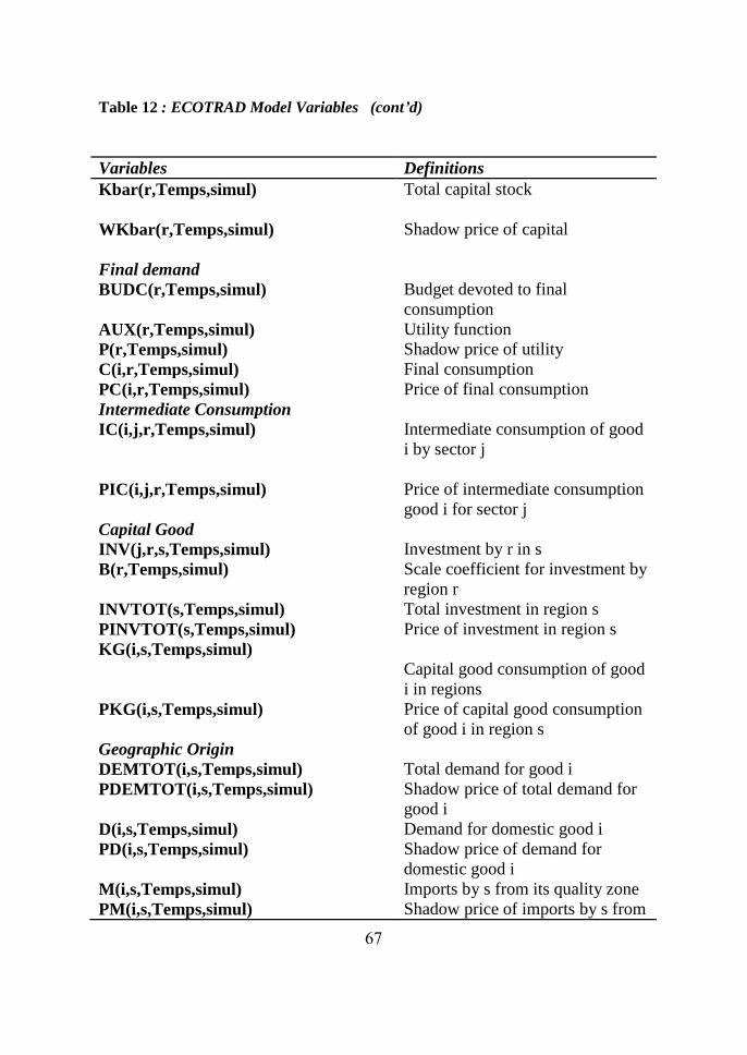
67

Table 12 : ECOTRAD Model Variables (cont’d)

Variables Definitions

Kbar(r,Temps,simul) Total capital stock

WKbar(r,Temps,simul) Shadow price of capital

Final demand

BUDC(r,Temps,simul) Budget devoted to final

consumption

AUX(r,Temps,simul) Utility function

P(r,Temps,simul) Shadow price of utility

C(i,r,Temps,simul) Final consumption

PC(i,r,Temps,simul) Price of final consumption

Intermediate Consumption

IC(i,j,r,Temps,simul) Intermediate consumption of good

i by sector j

PIC(i,j,r,Temps,simul) Price of intermediate consumption

good i for sector j

Capital Good

INV(j,r,s,Temps,simul) Investment by r in s

B(r,Temps,simul) Scale coefficient for investment by

region r

INVTOT(s,Temps,simul) Total investment in region s

PINVTOT(s,Temps,simul) Price of investment in region s

KG(i,s,Temps,simul)

Capital good consumption of good

i in regions

PKG(i,s,Temps,simul) Price of capital good consumption

of good i in region s

Geographic Origin

DEMTOT(i,s,Temps,simul) Total demand for good i

PDEMTOT(i,s,Temps,simul) Shadow price of total demand for

good i

D(i,s,Temps,simul) Demand for domestic good i

PD(i,s,Temps,simul) Shadow price of demand for

domestic good i

M(i,s,Temps,simul) Imports by s from its quality zone

PM(i,s,Temps,simul) Shadow price of imports by s from

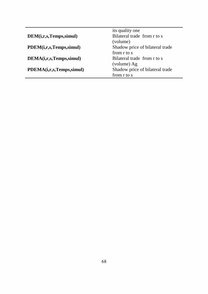
68

its quality one

DEM(i,r,s,Temps,simul) Bilateral trade from r to s

(volume)

PDEM(i,r,s,Temps,simul) Shadow price of bilateral trade

from r to s

DEMA(i,r,s,Temps,simul) Bilateral trade from r to s

(volume) Ag

PDEMA(i,r,s,Temps,simul) Shadow price of bilateral trade

from r to s

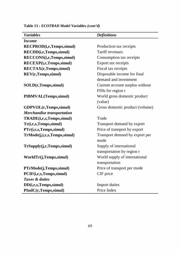
69

Table 13 : ECOTRAD Model Variables (cont’d)

Variables Definitions

Income

RECPROD(i,r,Temps,simul) Production tax receipts

RECDD(i,r,Temps,simul) Tariff revenues

RECCONS(i,r,Temps,simul) Consumption tax receipts

RECEXP(i,r,Temps,simul) Export tax receipts

RECTAX(r,Temps,simul) Fiscal tax receipts

REV(r,Temps,simul) Disposable income for final

demand and investment

SOLD(r,Temps,simul) Current account surplus without

FDIs for region r

PIBMVAL(Temps,simul) World gross domestic product

(value)

GDPVOL(r,Temps,simul) Gross domestic product (volume)

Merchandise transportation

TRADE(i,r,s,Temps,simul) Trade

Tr(i,r,s,Temps,simul) Transport demand by export

PTr(i,r,s,Temps,simul) Price of transport by export

TrMode(j,i,r,s,Temps,simul) Transport demand by export per

mode

TrSupply(j,r,Temps,simul) Supply of international

transportation by region r

WorldTr(j,Temps,simul) World supply of international

transportation

PTrMode(j,Temps,simul) Price of transport per mode

PCIF(i,r,s,Temps,simul) CIF price

Taxes & duties

DD(i,r,s,Temps,simul) Import duties

PIndC(r,Temps,simul) Price Index

70

Model equations

The equations of the model are summarized in the appendix. In what follows,

we present the structure of production, the commodity flows, and the model

shocks.

Structure of Production

The production technology is a Leontif production function characterized by

five (5) production factors (Capital, Unskilled, Skilled, Land and Natural

Resources). This is expressed by the Figure below. We have three Agents

(government, household, firm). The firm produced the mean of production

using composite intermediate input substitute to value added based on

endowment commodities. This is illustrated in Figure 21.

Figure 21. Structure of Production

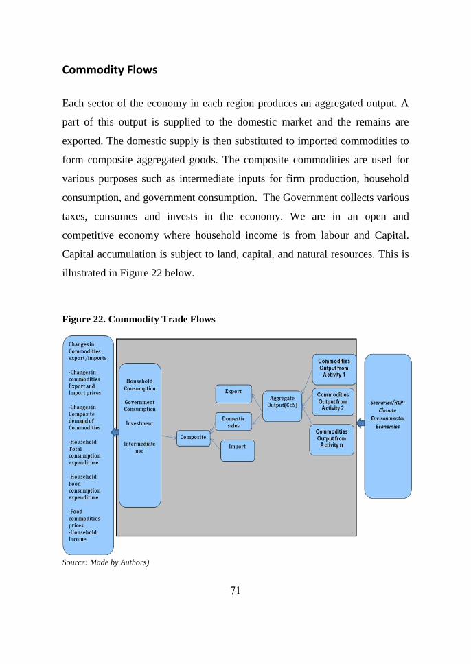
71

Commodity Flows

Each sector of the economy in each region produces an aggregated output. A

part of this output is supplied to the domestic market and the remains are

exported. The domestic supply is then substituted to imported commodities to

form composite aggregated goods. The composite commodities are used for

various purposes such as intermediate inputs for firm production, household

consumption, and government consumption. The Government collects various

taxes, consumes and invests in the economy. We are in an open and

competitive economy where household income is from labour and Capital.

Capital accumulation is subject to land, capital, and natural resources. This is

illustrated in Figure 22 below.

Figure 22. Commodity Trade Flows

Source: Made by Authors)

72

Model Shocks

For the impact assessment and following the structure of supply and demand,

three main shocks are implemented in the model.

Reference Scenarios

This refers to the Business as Usual (BUA) scenario. It defines the normal

trend with the implementation of ECOWAS common tax policy (CET).

This is explicitly expressed by:

( , , , , ) (1 ( , , , 1))* . ( , , 1, )taxEXPend i r s temps sim ctax i r s temps RECEXPl i r temps sim

Where ( , , , 1)ctax i r s temps are changes in the value of applied tax?

Changes in agricultural land allocation

Indeed, climate change will affect agricultural arable land and perhaps

reduce the land area used for this purpose. The reduction of

agricultural land will obviously induce changes in land allocation per

cultivated crops. Following the model production structure, the land is

considered as a production factor. In the model, all factors of

production are substituted using a Constant Elasticity of Substitution

(CES) relation. Changes in agricultural land allocation will induce

changes in aggregated output which is the mean change in agricultural

domestic output production. Thus, following commodity flows,

changes in domestic supply in return will affect the quantity and prices

of commodities imported, exported and consumed. The impact of

occur changes in agricultural crops land allocation is implemented in

the model through the following equation:

. ( , , , ) (1 ( , , 1))* . ( , , 1, )TE l j r temps sim chland j r temps TE l j r temps sim

Where ( , , 1)chland j r temps is the percentage changes in agricultural

land allocation per agricultural commodity, and

73

. ( , , , )TE l j r temps sim is the size of allocated land per cropping

system.

Changes in agricultural water allocation.

Indeed, following the model production structure, water is considered as an

intermediate input. Intermediate inputs play a key role in aggregated output

production. Climate change will affect water availability and perhaps water

allocation among end users. This is assessed through the water allocation

model namely ECOWAT. The impact of changes in agricultural water

allocation is expressed by the following equation

74

. ( , , , , ) (1 ( , , , ))* . ( , , , , )IC l j j r temps sim cwater i j r temps IC l i j r temps sim

Where:

( , , , )cwater i j r temps is changes in water usage per agricultural

commodity and per region and . ( , , , , )IC l i j r temps sim is water usage.

Water is an intermediate input in the model

Changes in the domestic supply of agricultural commodities.

Changes in domestic production are combined effects of changes in

cropping system yield and land allocation obtained from land

allocation model. In the model, the induced changes in domestic

output are implemented by the following equation:

. ( , , , ) (1 ( , , 1))* . ( , , 1, )Y l j r temps sim cpro j r temps Y l j r temps sim ;

Where

( , , 1)cpro j r temps is changes in domestic agricultural commodities’

production and . ( , , , )Y l j r temps sim is the level of domestic agricultural

firm production.

AQUACROP-ECOLAND-ECOWAT-ECOTRAD Models Integration

For the comprehensive impact assessment of climate change impact on food

security and trade flows, this section presents the overview of integrating the

crop model (AQUA-CROP) with the land Allocation model (ECOLAND), the

water allocation model (ECOWAT) and the trade model (ECOTRAD). This is

done through soft-link. Thus, AQUA-CROP estimates crop yield data under

various climate 3 majors’ trajectories. The first two trajectories are made of 2

Representative Concentration Pathways (RCP) define by IPCC namely

RCP4.5 and RCP8.5 while the third trajectory define climate change

adaptation strategy policy scenario. Thus, for each scenario, the obtained yield

is in turn used in ECOLAND as previously described. It should be recalled

75

that ECOLAND model estimates the cost-effectiveness of land size that

should be allocated to each cropping system and as well as the domestic crop

supply under a different scenario. In the model, crop prices, crop revenue and

livestock prices are taken as exogenous variables or parameters. These

variables are outputs from the hydro-economic model (ECOWAT). In

ECOWAT, crop water requirement, land allocation, and livestock population

are key inputs, which are generated from AQUA-CROP and ECOLAND as

outputs. Therefore, ECOLAND and ECOWAT are linked through

interchanging crop prices, crop revenue and livestock prices, as well as

through land allocation data (Fig 29).

ECOTRAD, a modified version of MIRAGE World Trade Model

communicates with ECOLAND and ECOWAT. This communications is via

land use as changes and crop water allocation. These changes are exogenous in

ECOTRAD and derive from ECOLAND and ECOWAT. Further, ECOTRAD

generates price data that enters ECOLAND and ECOWAT as parameters. This

is also illustrated in Figure 23 below.

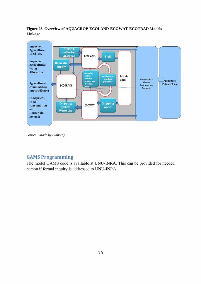
76

Figure 23. Overview of AQUACROP-ECOLAND-ECOWAT-ECOTRAD Models

Linkage

Source: Made by Authors)

GAMS Programming The model GAMS code is available at UNU-INRA. This can be provided for needed

person if formal inquiry is addressed to UNU-INRA.

77

Conclusion

It is commonly recognized that climate change constitutes a veritable threat to

African development and particularly to ECOWAS countries. However, despite many

attempts to quantify the impact of climate in the region’s key development pillars

such as agriculture, trade, and food security, very limited work has been done to

evaluate the spatial and temporal distribution of the impact of climate change and

fully integrate the nexus between production and consumers’ patterns. This could

reduce uncertainty in obtaining the results of impact assessment of climate change

and improve decision-making.

Therefore, to assess the impact of climate change on agricultural production, the

proposed Integrated Assessment framework has attempted to incorporate the spatial

and temporal changes which is caused by climate change on farming production

system as well as the inputs (i.e. quantities and prices). This includes quantities and

prices of land, water resources, fertilizers, labour, technology and the like. In

addition, the framework has included the nexus linkage between resources end users.

These are illustrated in both the dynamic land allocation model (ECOLAND) and the

hydro-economic model (ECOWAT).

However, to assess the impact of climate change on agricultural commodity trade and

food security, the proposed framework has incorporated the intra-market linkage

between ECOWAS countries and the Rest of the World and fully integrated the

multiple dimension of food security definition. This includes the condition of food

availability, food accessibility, food utilization and stability. Given the limitation of

using trade model as a single model set to analyse the impact of climate change on

agricultural trade and food security, the framework offers the possibility to fully

integrate the trade model (ECOTRAD) with ECOLAND and ECOWAT.

By implementing this, the framework requested intensive data but fully incorporated

spatial and temporal producers, consumers and market behaviours information for

robust analysis and improved decision-making options to enhance adaptation policies

in boosting the region’s resilience to climate change.

78

References Claudia, R.; Tingju, Z.; Ximing, C.;Jawoo ,K; Dingbao, W.; 2010.Climate

Change Impacts on Food Security in Sub-Saharan Africa Insights from

Comprehensive Climate Change Scenarios. Washington, DC, International

Food Policy Research Institute (IFPRI).

Food and Agriculture Organisation (FAO) 2010. Climate Change Implication

for Food Security and Natural Resources Management In Africa. Report on

Twenty-Sixth Regional Conference For AFRICA. Luanda, 81-82. Angola, 03

– 07 May 2010.

Food and Agriculture Organisation (FAO) 2009. Climate Change in Africa: The

threat to agriculture. FAO Report

Frank, A. W and Shokhrukh-Mirzo, J. 2011.AMUDARYA BASIN With

Tradeoff Between, Season, Countries, crops, power. Water Economics and

Policy Research paper.

IPCC 2014. Climate Change 2014: Impacts, Adaptation, and Vulnerability

.IPCC WGII AR5 Technical Summary. Chapter 22: PP 1202-1243.

Kutcher, G P, and Scandizzo, P .L. 1981. The Agricultural Economy of

Northeast Brazil. The Johns Hopkins University Press, Baltimore, and

London, 1981

Nelson, G.C., Rosegrant, M.W., Palazzo, A., Gray, I., Ingersoll, C., Robertson,

R. & Tokgoz, S. 2010. Food security, farming, and climate change to 2050:

scenarios, results, policy options. Washington, DC, International Food Policy

Research Institute (IFPRI).

Yvan, D. and Hugo, V. 2007. MIRAGE, Updated Version of the Model for

Trade Policy Analysis: Focus on Agriculture and Dynamics. CEPII, Working

Paper No 200

UNU-INRA Contact

United Nations University Institute for Natural Resources in Africa

(UNU-INRA)

Second Floor, International House,

Annie Jiagge Road, University of Ghana, Legon

Accra, Ghana

Private Mail Bag,

Kotoka International Airport, Accra, Ghana

Tel: +233-302- 213850. Ext. 6318

Email: inra@unu.edu

Website: www.inra.unu.edu

MATE MASIE

“What I hear, I

keep”-Symbol of

wisdom, knowledge

and understanding.

NEA ONNIMNO SUA

A, OHU

“He who does not know

can know from learning,

-Symbol of life-long

education and continued

NYANSAPO

“Wisdom knot” – Symbol of

wisdom, ingenuity, intelligence

and patience.