ISSN 0280-5316ISRN LUTFD2/TFRT--5687--SE

Modelling of MicroturbineSystems

Staffan Haugwitz

Department of Automatic ControlLund Institute of Technology

May 2002

Document nameMASTER THESISDate of issueMay 2002

Department of Automatic ControlLund Institute of TechnologyBox 118SE-221 00 Lund Sweden Document Number

ISRN LUTFD2/TFR--5687--SESupervisorAnders Rantzer and Hubertus Tummescheit (LTH)Göran Stångberg (Turbec AB)

Author(s)Staffan Haugwitz

Sponsoring organization

Title and subtitleModelling of Microturbine Systems (Modellering av mikroturbinsystem)

AbstractThe thesis describes the development of a dynamic model of a microturbine system. The thesis is done inclose cooperation with Turbec AB and the model is adjusted, tuned and verified against theirmicroturbine T100. The microturbine unit consists of a compressor and a turbine connected on a singleshaft to a high-speed generator. Moreover there is a combustion chamber, a recuperator and a gas/waterheat exchanger. A control system regulates the speed, the temperature and the electric power. To controlthe frequency, voltage and current of the outgoing power, the microturbine uses power electronics.The model is to be used in the research and development department at Turbec AB. Possible applicationsare in areas as control strategies, dynamic performance verification, operator training and controlsoftware/hardware verification. Since the potential applications are so different, the emphasis throughoutthe thesis has been on a general model that can be used in as many different operating ranges as possible.This should be done while retaining a high degree of accuracy at the most common scenario, running onfull load. The emphasis has also been on the functionality and accuracy of the complete model over moredetailed modelling of each component.In the thesis, the thermodynamic theory of each component is described and how it is modelled inModelica. The microturbine model in the thesis covers the gas turbine unit, the control systemand the mechanical part of the generator. The electric part of the generator and the powerelectronics are not included in the model, due to the limited time of the project. The thesis alsodiscusses the well-known problems with modelling as e.g. discretisation and interpolation.The model uses components from the ThermoFluid library, the Modelica standard library and theMaster’s thesis of Perez (2001).Static verification has been done with data from DSA, a steady state calculation program, whichaccurately represents the real microturbine. The Modelica model developed in the thesis has beenfound very accurate at the main operation range (100 kW down to 50 kW), with an average errorof 0.6 % of the 13 most important thermodynamic variables at full load, 100 kW. Dynamicverification in three different scenarios has been done against the real microturbine and the modelshows a good fit to the measured data.

Keywords

Classification system and/or index terms (if any)

Supplementary bibliographical information

ISSN and key title0280-5316

ISBN

LanguageEnglish

Number of pages55

Security classification

Recipient’s notes

The report may be ordered from the Department of Automatic Control or borrowed through:University Library 2, Box 3, SE-221 00 Lund, SwedenFax +46 46 222 44 22 E-mail ub2@ub2.se

Modelling ofMicroturbine Systems

Staffan HaugwitzMaster’s Thesis

Lund Institute of TechnologyMay 2002

2

3

Table of Content

PREFACE ..................................................................................................................................................... 5

NOMENCLATURE ..................................................................................................................................... 6

1. INTRODUCTION .................................................................................................................................... 7

1.1 Background....................................................................................................................................... 71.2 The project description ..................................................................................................................... 7

2. GAS TURBINES....................................................................................................................................... 8

2.1 The Brayton cycle ............................................................................................................................. 82.2 The non-ideal Brayton cycle ........................................................................................................... 112.3 Regeneration................................................................................................................................... 11

3. THE T100 MICROTURBINE SYSTEM.............................................................................................. 12

3.1 The T100 microturbine ................................................................................................................... 123.2 Operation Modes ............................................................................................................................ 143.3 Extra dynamics ............................................................................................................................... 153.4 Bypass............................................................................................................................................. 15

4. SIMULATION TOOLS ......................................................................................................................... 15

4.1 Selecting the tools ........................................................................................................................... 154.2 Dymola ........................................................................................................................................... 164.3 Modelica ......................................................................................................................................... 184.4 The ThermoFluid Library ............................................................................................................... 18

5. THERMODYNAMIC THEORY AND MODELLING ...................................................................... 22

5.1 The compressor equations .............................................................................................................. 225.2 The compressor model in Modelica................................................................................................ 245.3 The turbine equations ..................................................................................................................... 305.4 The turbine model in Modelica....................................................................................................... 315.5 The heat exchanger......................................................................................................................... 345.6 Pipes and pressure loss models ...................................................................................................... 365.7 The heat exchanger model .............................................................................................................. 365.8 The combustion chamber................................................................................................................ 385.9 The temperature sensor .................................................................................................................. 405.10 The Generator, Friction losses and Auxiliary equipment models................................................. 415.11 Flow Sources and Reservoirs ....................................................................................................... 415.12 The Control System....................................................................................................................... 42

6. SIMULATIONS AND VERIFICATION ............................................................................................. 42

6.1 Simulations ..................................................................................................................................... 426.2 Static verification............................................................................................................................ 456.3 Dynamic verification ...................................................................................................................... 47

7. CONCLUSIONS AND SUMMARY ..................................................................................................... 51

7.1 Static verification............................................................................................................................ 527.2 Dynamic verification ...................................................................................................................... 527.3 Valid operating ranges for the model ............................................................................................. 52

8. POSSIBLE APPLICATIONS AND FUTURE WORK....................................................................... 52

REFERENCES ........................................................................................................................................... 53

4

5

PrefaceThis thesis is concerned with the development of a thermodynamic simulation model of amicroturbine. It was written at Turbec AB in cooperation with the institution of AutomaticControl at Lund Institute of Technology. Turbec AB is a newly founded company (1998), jointlyowned by Volvo Aero AB and ABB. In 1992 Volvo presented the Environmental Concept Car(ECC), which had a turbine-generator system based on a high-speed generator directly coupledwith a simple single-shaft gas turbine. The gas turbine constantly charged batteries, whichpowered the vehicle.The knowledge and experience from the mobile microturbines led to the development of a newtechnology, stationary combined heat and power (CHP) plants on a miniature scale. Volvobrought in ABB as a partner and formed the independent company Turbec AB. The first productof the company is the T100, a microturbine that can produce 100 kW of electric power andanother 167 kW of heat with a total efficiency of 80%. The market of microturbines did not existuntil 5 years ago, when Honeywell presented their first product. Now the market is growingrapidly. Due to confidentiality, some of the figures in this thesis are presented rescaled andwithout axes.

I would like to thank my tutors Anders Åberg (Turbec AB), Hubertus Tummescheit (LTH) andAnders Rantzer (LTH) for their help and enthusiasm throughout my work with the thesis.

Lund, May 2002Staffan Haugwitz

6

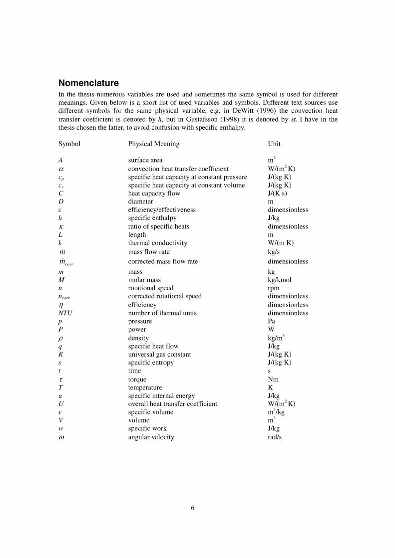
NomenclatureIn the thesis numerous variables are used and sometimes the same symbol is used for differentmeanings. Given below is a short list of used variables and symbols. Different text sources usedifferent symbols for the same physical variable, e.g. in DeWitt (1996) the convection heattransfer coefficient is denoted by h, but in Gustafsson (1998) it is denoted by α. I have in thethesis chosen the latter, to avoid confusion with specific enthalpy.

Symbol Physical Meaning Unit

A surface area m2

α convection heat transfer coefficient W/(m2 K)cp specific heat capacity at constant pressure J/(kg K)cv specific heat capacity at constant volume J/(kg K)C heat capacity flow J/(K s)D diameter mε efficiency/effectiveness dimensionlessh specific enthalpy J/kgκ ratio of specific heats dimensionlessL length mk thermal conductivity W/(m K)m& mass flow rate kg/s

corrm& corrected mass flow rate dimensionless

m mass kgM molar mass kg/kmoln rotational speed rpmncorr corrected rotational speed dimensionlessη efficiency dimensionlessNTU number of thermal units dimensionlessp pressure PaP power Wρ density kg/m3

q specific heat flow J/kgR universal gas constant J/(kg K)s specific entropy J/(kg K)t time sτ torque NmT temperature Ku specific internal energy J/kgU overall heat transfer coefficient W/(m2 K)v specific volume m3/kgV volume m3

w specific work J/kgω angular velocity rad/s

7

1. Introduction

1.1 BackgroundIn this section, I will briefly explain the market idea behind the microturbine systems. How comethat these small units can compete with larger power plants?

In recent years a slow deregulation of the power generation market has taken place throughout theworld. It is open to anyone to produce its own electricity and to export it to others. The market isalso open to international corporations and monopolies in many countries are breaking up. Thepower corporations that produce energy in large complex facilities are now exposed tocompetition from small-scale production of power on site where the need is. State-owned powercompanies that were controlled by the government are now sold out on the stock market. The newowners tend to have a shorter perspective and value short- or medium-time profits. Long-termcommitments are less frequent. The private companies do not want to maintain a large productionbuffer to assure that enough power is produced in case of extreme weather or other crisis. Thepower demand changes quickly in size and location. The prize on power changes also rapidlyworld wide due to speculations, politics and natural disasters.

All these changes make it harder for companies to justify the investments that a new full-scalepower plant requires. An interesting example is California, USA where almost no new powerplants have been built during the 8 years since the power market was deregulated in 1996; asituation which made the power shortages during January in 2001 more severe.

This development has lead to a new interest in small-scale power plants that are easy and quick toinstall, with low cost and a short payback time. The power production can be adjusted to thecurrent demand and if the demand increases over time, another turbine can be installed. Thecompanies do not need to take the full investment that a larger power plant would take. Small-scale power production can be viewed with the motto: invest as you grow.

Small-scale power plants are nothing new. But now it can be combined with water heating, thusincreasing the total efficiency from 30 to 80 %! The combination of power and heat (CHP)generation is therefore essential to the success of the microturbine system.

The development of small-size on-site power plants increases also the flexibility in the powergeneration, e.g. when they are placed in clusters and connected into networks to serve manycustomers at many different locations. These distributed micro-grids can e.g. be operated ascentralized systems monitored from a single location.

1.2 The project descriptionThe microturbine T100 CHP is now being sold all over the world, with new versions andapplications coming up. In order to verify new control strategies, e.g. how to control fourmicroturbines connected in parallel, it is essential to have a reliable model to evaluate the staticand dynamic effects. When designing new braking strategies for over speed protection it is alsoessential to have a model to work with. With a simulation model they can try these ideas out in asafe and timesaving way, instead of using a real machine. The purpose of this thesis is to give theengineers this simulation model.

As will be explained in chapter on Simulation Tools, no existing model at Turbec covers allaspects. The objective with the thesis is therefore to develop a thermodynamic simulation model

8

for later use in various applications, e.g. the software development of the control system. Otherapplications might be to test hardware components from the control system connected to the realI/O interface, but with a PC doing hardware in the loop simulation. The model can also be used asa tool in operator training, i.e. how to operate the machine with its user interface but with asimulation model instead of the real microturbine.After some discussions (see the chapter on Simulation Tools) a decision was made to write themodel in the language Modelica and use the simulation program Dymola from Dynasim AB,Lund. The model should also be extendable to cover the power electronics in a future work. Itshould be possible to export the model to other simulation environments as e.g. Matlab/Simulink.The model is to be verified against other simulation programs and real data from experiments.The model should be as complete as possible, including extra components, e.g. the recuperatorand gas/water heat exchanger.

This thesis is a continuation of the Master’s thesis by Perez (2001), where the basic structure ofgas turbine modelling was outlined. The model structure of some of the components, e.g. thecompressor and the turbine, was reused in the new model. Even though the machine modelled inthat thesis was physically larger and produced 600 kW of power, the thermodynamic equationsare the same. All the parameters, e.g. the ones containing the characteristics of e.g. compressorand turbine, had to be changed. The reuse of Perez’s models saved large amounts of time andmore efforts could therefore be made in parameter tuning and verification of the model,something that was beyond the scope of his thesis. Still one must emphasize that tuning adynamic model with hundreds of parameters is a very delicate matter and the most importantobjective is to achieve a sound and reliable dynamic model with a thorough physical background.

In the chapters about Modelica, ThermoFluid and the derivation of the thermodynamic equationsI have a similar approach to the one used in Perez (2001) since our base sources e.g. Cohen(1998) and Cengel (1999) are the same. I want to avoid repeating the same texts and equations asin Perez (2001), but in order to make my thesis complete and understandable to read withouthaving the references, I have decided to include similar text and derivations.

2. Gas TurbinesIn this chapter I will describe the general features of a gas turbine, the governing equations andthe different steps in the ideal and the real Brayton cycle.

2.1 The Brayton cycleThe figure below shows the ideal open Brayton cycle. Fresh air is drawn into to compressor.

9

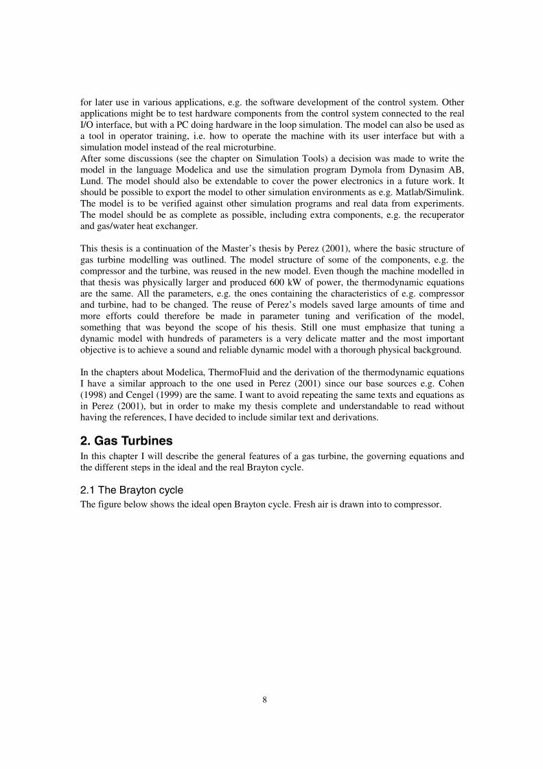
Figure 1: An open ideal Brayton cycle, Cengel (1998)

The compressor at stage 1 increases the pressure of the fresh air with a factor 4 – 20 depending onits size and construction. At stage 2 the high-pressure air and fuel are mixed and burnt in thecombustion chamber at a constant pressure. The very hot flue gas enters the turbine at stage 3 andforces the turbine to rotate, thus producing mechanical work. During this procedure the flue gasexpands to lower pressure and larger volume, therefore the turbine is also called an expander. Atstage 4 the exhaust gas is released to the surroundings. Since there are mass flows in and out ofthe process, it is called an open cycle. It can be remodelled as a closed cycle, i.e. there is no massflow in or out of the process, by doing two approximations in the process. Firstly, the combustionchamber is replaced by a heat exchanger where the air is heated to the same temperature as itwould get during combustion, but now no fuel is added. Secondly, another heat exchanger isplaced between stage 4 and 1 such that the exhaust gas is cooled by the surroundings to thetemperature at stage 1. Then the same fluid is used throughout the process, hence the name closedcycle. The closed cycle is often used for thermodynamic analysis.

10

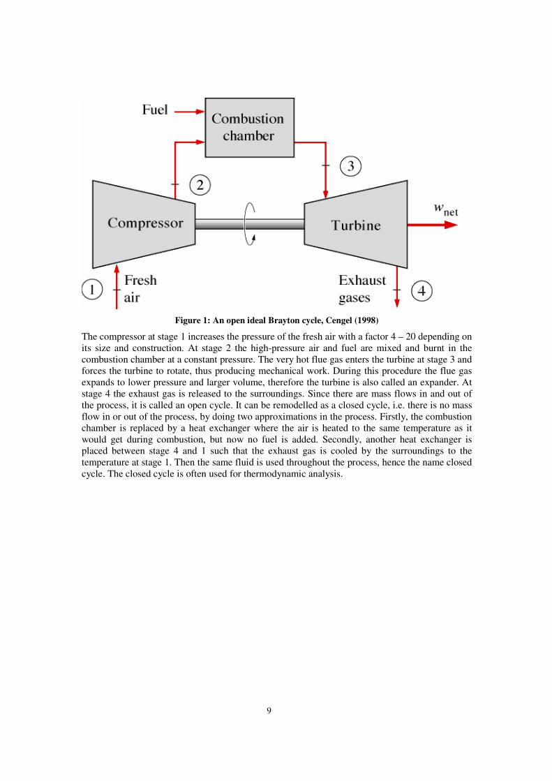
Figure 2: T-s and p-ν diagrams for the ideal closed Brayton cycle, Cengel (1998)

In the figure to the right above, we can see how the pressure and specific volume changethroughout the cycle and in the figure to the left above, the change in temperature and entropy isshown. Specific volume is defined as the inverse of the density, i.e. how much volume a unitmass occupies. During compression, the pressure and temperature increase. The pressure increasetends to increase the density, whereas the increase in temperature tends to decrease the density.The total effect is a small increase in density, which corresponds to a small decrease in specificvolume. In an ideal cycle the compression is isentropic, i.e. adiabatic (no heat loss) and internallyreversible (the entropy does not change due to friction etc). Therefore the entropy is constant eventhough the temperature increases.In the combustion chamber heat is added to the gas at constant pressure. The density decreasesand the specific volume and temperature are increased. Entropy is also increased, sincecombustion is not a reversible process. In the turbine the situation is the opposite of thecompressor; the pressure decreases and specific volume increases. The temperature decreases andin an ideal expansion the entropy is constant.

From basic thermodynamics we know that the encircled area in the p-v diagram represents theproduced net work of the gas turbine. The efficiency of the gas turbine is the ratio of produced network and added heat power. The efficiency can be rewritten to the following, according to Cengel(1998).

κκη/)1(

11 −−==

pin

net

rq

w

where rp is the pressure ratio in the turbine and κ is the ratio of specific heats. The higher pressureratio of the gas turbine, the higher is its efficiency. The equation is only valid for ideal gasturbines with no friction and reversible processes.

(2.1.1)

11

2.2 The non-ideal Brayton cycleIn reality compression and expansion are not ideal processes. Friction and turbulence cause anincrease in entropy, which can be seen in the figure below. There are also pressure drops in pipesand during combustion.

Figure 3: The deviation of an actual gas turbine from the ideal Brayton cycle as a result ofirreversibilities, Cengel (1998)

2.3 RegenerationThere are large gains to be made if some of the heat in the exhaust gas leaving the turbine can bereused, instead of being rejected to the surroundings. This occurs in a regenerator, often called arecuperator. The hot exhaust gas can preheat the fresh air going into the combustion chamber,thus reducing the fuel requirements for the same net work output, Cengel (1998). The efficiencycan now be written as:

kkpr

T

T /)1(

3

11 −

−=η

where T1 and T3 are the temperatures before compression (the ambient temperature) and aftercombustion respectively. The equation gives that the higher difference between the temperature atwhich heat addition (combustion) and heat rejection (exhaust gas leaves and fresh air comes in)occurs, the higher is the efficiency. The recuperator increases the combustion temperature, thusincreasing the efficiency. In the T100 microturbine, the increase in efficiency at full power load,100 kW, is from 17 % to 30 %! However, not all gas turbines can or should use a recuperator. Ifthe temperature of the fluid at the turbine outlet is lower than at the compressor outlet, the heatflow would go in the wrong direction. This occurs in gas turbines with very high pressure ratios,since the temperature increase/decrease in the compressor/turbine depends on the pressure ratio atwhich they operate, see equation (5.1.8). The initial cost will also be higher and the system willbe more complex and likely to failures. If the gas turbine is only used as a back-up and run for afew days a year, a recuperator might not be advantageous.

(2.3.1)

12

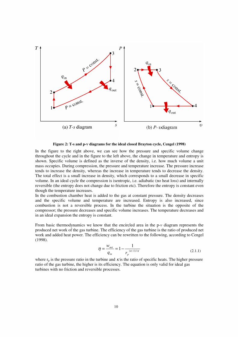
Figure 4: An ideal Brayton cycle with a regenerator, Cengel (1998)

In larger gas turbines there are additional possible stages, as for example intercooling and twostage expansion and compression. These stages will increase the total efficiency, but will makethe gas turbine more expensive to manufacture and more complex. For smaller gas turbines theseadditional features usually do not pay off.

3. The T100 microturbine systemIn this chapter I will describe the T100 microturbine and explain some special features that makeit different from normal gas turbines.

3.1 The T100 microturbineThe microturbine T100 is a power generation system that is based on a combination of a smallgas turbine and a directly driven high-speed generator. The generator is placed on the same shaftas the compressor and the turbine. No gearbox is therefore needed and the system uses only twobearings, reducing the friction losses to a minimum. The microturbine technology is described inMalmquist (1999).

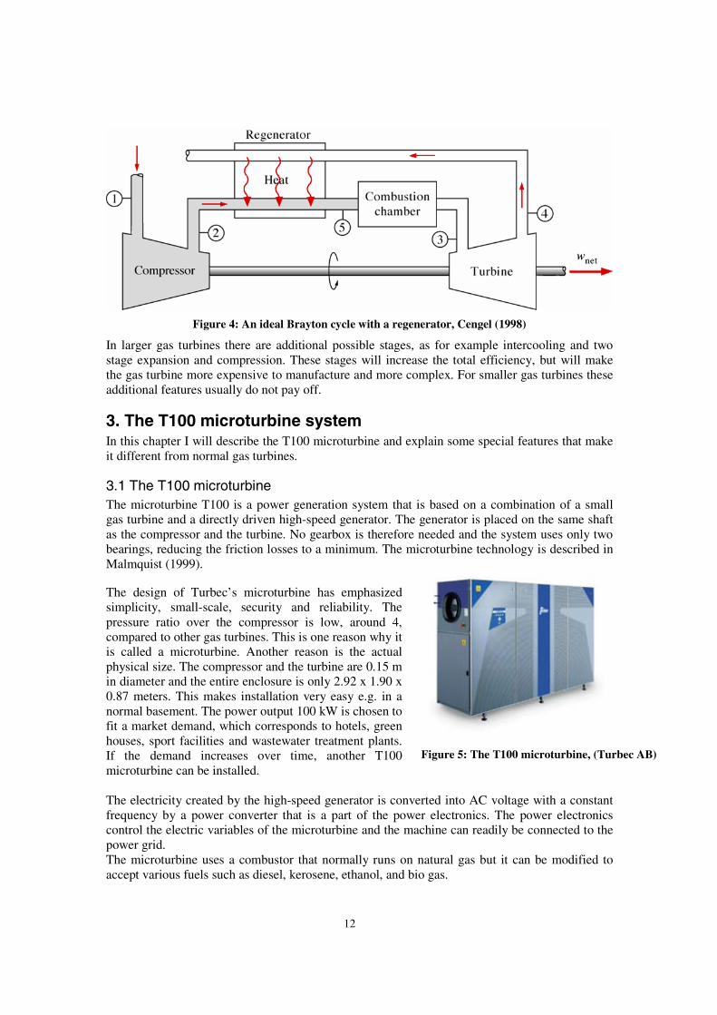
The design of Turbec’s microturbine has emphasizedsimplicity, small-scale, security and reliability. Thepressure ratio over the compressor is low, around 4,compared to other gas turbines. This is one reason why itis called a microturbine. Another reason is the actualphysical size. The compressor and the turbine are 0.15 min diameter and the entire enclosure is only 2.92 x 1.90 x0.87 meters. This makes installation very easy e.g. in anormal basement. The power output 100 kW is chosen tofit a market demand, which corresponds to hotels, greenhouses, sport facilities and wastewater treatment plants.If the demand increases over time, another T100microturbine can be installed.

The electricity created by the high-speed generator is converted into AC voltage with a constantfrequency by a power converter that is a part of the power electronics. The power electronicscontrol the electric variables of the microturbine and the machine can readily be connected to thepower grid.The microturbine uses a combustor that normally runs on natural gas but it can be modified toaccept various fuels such as diesel, kerosene, ethanol, and bio gas.

Figure 5: The T100 microturbine, (Turbec AB)

13

An exhaust gas recuperator is included that improves the efficiency of the system substantially.The machine is designed to run for a long time on full load and the extra investment that therecuperator requires is quickly saved. The recuperator is also especially beneficial due to the lowpressure ratio of the T100. The difference in temperature after the compressor and after theturbine is large and the recuperator can then transfer large amounts of heat from the exhaust gasto the compressed air; see the regeneration section.

There is also a gas/water heat exchanger, where water is heated by the exhaust gases coming fromthe recuperator. The hot gas has a heat potential that can deliver 167 kW at full load to the hotwater system. With an electric efficiency of 30 % and the extra gas/water heat exchanger, thetotal efficiency is about 80 %! The water can then be used to heat buildings. In countries whereheat is in abundance, an absorption chiller can replace the gas/water heat exchanger to provide airconditioning. This application will shortly be introduced in the T100 microturbine.

A very important property of the T100 is its low emissions. The whole system is designed andoptimized to minimize all harmful emissions. All the individual components are optimized for acertain speed or temperature where the losses are at a minimum and the efficiency at a maximum.The control system meticulously controls the speed and combustion temperature of themicroturbine and keeps them constant to ensure stable and complete combustion with as lowemissions as possible. The exhaust gases are actually so clean that the microturbine can be usedinside green houses. In this application the T100 can supply power to the grid and heat tomaintain the high temperature in the green house, while carbon dioxide in the exhaust gases aresupplied to the plants as fertilizer to increase growth. In some green houses, gas boilers are usedto provide the plants with heat and this extra carbon dioxide, but the demand of heat is lower thanthe demand of carbon dioxide so much heat is wasted. Instead some of this heat can be used toproduce electricity by installing a T100 microturbine.

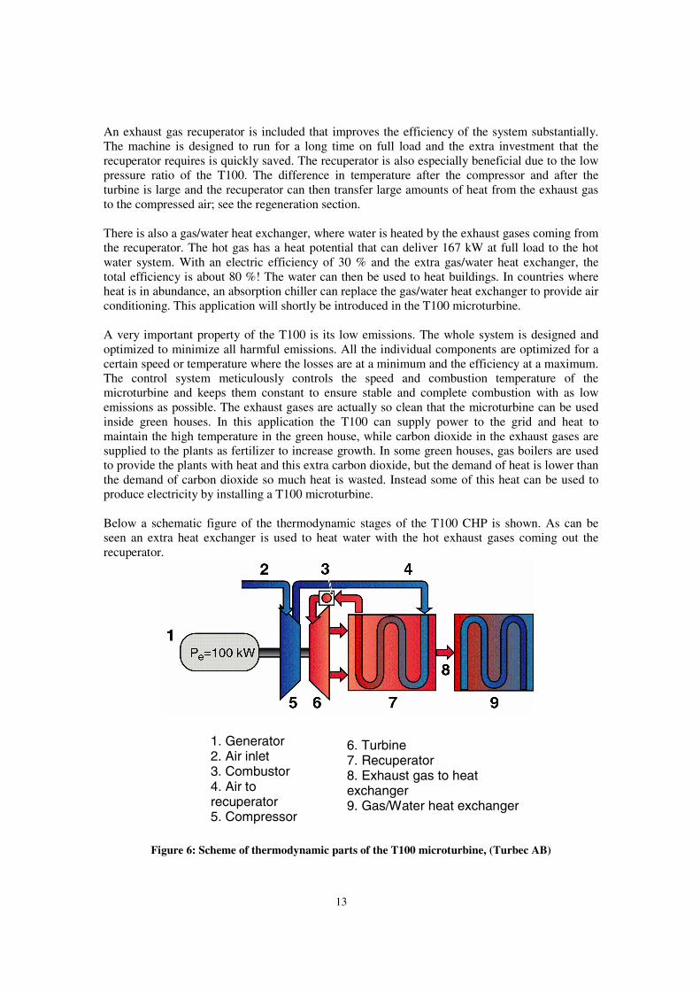
Below a schematic figure of the thermodynamic stages of the T100 CHP is shown. As can beseen an extra heat exchanger is used to heat water with the hot exhaust gases coming out therecuperator.

Figure 6: Scheme of thermodynamic parts of the T100 microturbine, (Turbec AB)

1. Generator2. Air inlet3. Combustor4. Air torecuperator5. Compressor

6. Turbine7. Recuperator8. Exhaust gas to heatexchanger9. Gas/Water heat exchanger

14

3.2 Operation ModesThe normal operation mode is the parallel mode, i.e. the microturbine produces heat and powerparallel to the power grid. The local power grid is connected to an outer power grid. If the T100produces more power than needed in the local power grid, it is exported via the outer grid. If itproduces less power, then the remaining power is taken from the outer grid. The owner candecide when and how much power the microturbine should produce depending e.g. on the priceof the power from the outer grid. During nights power from the outer grid is cheaper and then themicroturbine can be stopped.

The other important mode of operation, not yet fully implemented and tested, is the stand-alonemode. This means that the outer power grid has been disconnected due to some reasons, e.g.black-outs, power shortages and technical failures. Then the microturbine has the soleresponsibility to produce power to the local power grid. This puts very high demands on speedand reliability. The voltage and frequency needs to be kept constant regardless of the loads on thepower grid. In parallel mode, the control system is slow in order to keep the thermal fluctuationsin the machine to a minimum. In stand-alone mode there is no possibility to take such precautionssince the power output is the primary objective.

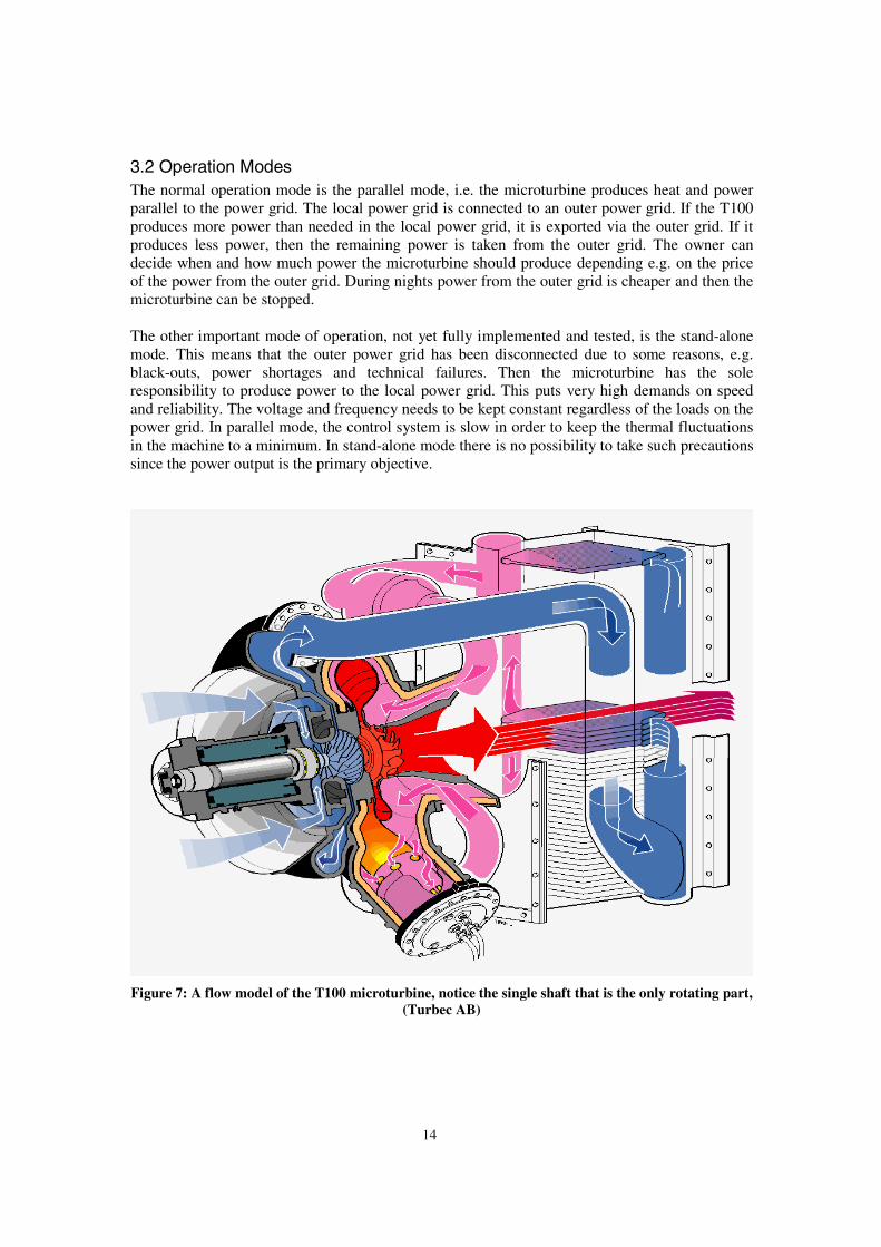
Figure 7: A flow model of the T100 microturbine, notice the single shaft that is the only rotating part,(Turbec AB)

15

3.3 Extra dynamicsA gas turbine consists of different components and when all components are put together someextra dynamics arise. The flow model of the T100 in figure 7 above gives a more detailed view ofhow the turbine works. Air is taken from the outside and flows around the generator into thecompressor in axial direction. The air is compressed and leaves in radial direction. The high-pressure air (blue pipes) is fed through the recuperator where it is preheated with the exhaust gas.Now at a much higher temperature (pink pipes) it is mixed with the fuel gas in the combustionchamber and burned. The flue gas enters the turbine radially and leaves in an axial direction (redpipes). The flue gas exchanges heat with the colder air in the recuperator and then leaves thefigure. The gas/water heat exchanger (not shown in the figure) is placed directly after therecuperator.

In an ideal machine the turbine would be a purely algebraic component with no dynamicsinvolved. Instead, when we include the turbine rotor and the turbine diffuser (the part directlyafter the turbine marked red in the figure above), we get some extra dynamics. The turbine rotorcan store thermal energy and when the temperature of the exhaust gas decreases, due to a loadchange, the rotor acts as small thermal reservoir with a limited amount of energy. The rotor speedis very high, so that the energy stored in the rotor is easily transferred to the gas, thus acting as afilter on the temperature dynamics. Due to the geometric design, the turbine diffuser serves as anextra heat exchanger, although a very poor one. The extra heat exchanger has a considerablysmaller effect than the recuperator, but along with the turbine rotor they have an interestingimpact on the dynamics. The actual effect can be seen in the verification section.

3.4 BypassThe T100 CHP microturbine produces heat through the gas/water heat exchanger. The amount ofheat produced is directly linked to the amount of electricity produced. In some cases the ownerwants to produce less heat than electricity. If too much heat is transferred to the water, the watermight boil and evaporate causing damage to the heat exchanger. Therefore the amount of heattransfer must be controlled in a way that does not interfere with the electricity production. Thesolution is a bypass system, where some or all exhaust gases are diverted around the gas/waterheat exchanger in a similarly way as a valve works. Due to time and the low priority given tobypass operations, there is no complete verified model of the bypass function in this thesis.

4. Simulation ToolsIn this chapter I will describe the tools I have used in the modelling of the microturbine. There aredifferent layers of tools. First there is the simulation language, the language the model is writtenin, e.g. Modelica. Then there are libraries e.g. ThermoFluid that contain complete submodels.And last there is a simulation program e.g. Dymola, that contains a graphical user interface,different solvers, plot functions and parameter settings.

4.1 Selecting the toolsThermodynamic models are often large and complex. They consist of volumes, flows but alsoelectronic components. There exist numerous simulation languages and programs e.g. Fortran,Matlab/Simulink and Modelica/Dymola to just mention a few of them. To make things morecomplicated there are several different simulation programs used within Turbec AB for differentpurposes and applications. For static simulations, a program called Dynamic Systems Analyzerv2.0 (DSA) is used. DSA is a program developed at Volvo Aero Corporation AB. With version2.0 only static simulations are possible. A very detailed model of the T100 with all components

16

and connections is used in simulations to get static results with high accuracy. The model hasthen been verified with experimental data and calibrated to further improve the model’s accuracy.

Matlab/Simulink is used to model the power electronics and control system including a coarsethermodynamic model. The problem with Matlab/Simulink is that the program does not modelflows well in general and flows in sudden changing directions in particular. Matlab/Simulinksupports causal modelling with fixed causality of inputs and outputs and hard work is needed toput the system in the order of an ordinary differential equation (ODE). The modelling is also notcomponent-oriented. More discussions can be found in the Modelica chapter. A third program,ICES, (Internal Combustion Engine Simulation), is used to create a dynamic model of themicroturbine engine. The program is written in Fortran and is component-oriented. The drawbackis that Fortran does not have a graphical user interface, which makes it harder to learn. Mostmodels are however written in Fortran and it is the most widely used modelling language in theindustry. The very useful library ThermoFluid is also a major incitement to choose Modelica asthe modelling language. Fortran does have a similar library for thermodynamic models but inother areas as e.g. electronics Modelica is better situated than Fortran. Models in Modelica canalso be transferred to other simulation environments as S-functions in Matlab/Simulink, whichICES cannot. It is possible to execute Fortran and C code in Matlab but to integrate the modelwith other Simulink models you need to convert the code into S-functions. In total this lead us tochoose Modelica as our choice of modelling language with ThermoFluid as a prime resource forthe basic blocks. In choosing Modelica we also chose Dymola as our simulation program sincethose two are closely linked. The company behind Dymola, Dynasim AB is also very active in thedevelopment of Modelica as the new language of modelling. After this initial discussion I willdescribe the different simulation tools used in this thesis.

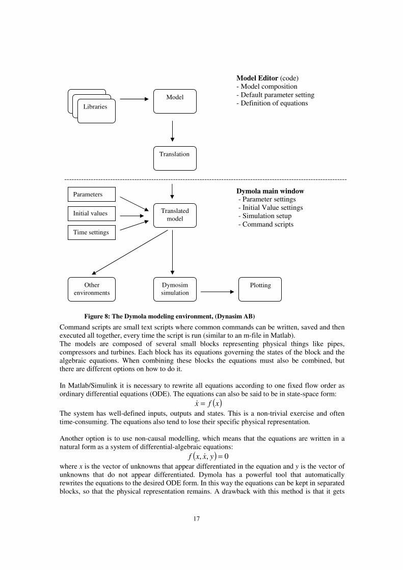
4.2 DymolaDymola, Dynamic Modeling Laboratory, is a simulation program consisting of a compiler,graphical user interface, numerical solvers and plot functions. For more information on Dymola,see the Dymola manual (2001) or their home page www.dynasim.se.The models are written in the Modelica language. Dymola generates the C code, which iscompiled and linked with the solver routines into a simulation executable, Dymosim. In theDymola Main Window parameters, initial conditions and simulation settings can be set.

17

Command scripts are small text scripts where common commands can be written, saved and thenexecuted all together, every time the script is run (similar to an m-file in Matlab).The models are composed of several small blocks representing physical things like pipes,compressors and turbines. Each block has its equations governing the states of the block and thealgebraic equations. When combining these blocks the equations must also be combined, butthere are different options on how to do it.

In Matlab/Simulink it is necessary to rewrite all equations according to one fixed flow order asordinary differential equations (ODE). The equations can also be said to be in state-space form:

( )xfx =&The system has well-defined inputs, outputs and states. This is a non-trivial exercise and oftentime-consuming. The equations also tend to lose their specific physical representation.

Another option is to use non-causal modelling, which means that the equations are written in anatural form as a system of differential-algebraic equations:

( ) 0,, =yxxf &

where x is the vector of unknowns that appear differentiated in the equation and y is the vector ofunknowns that do not appear differentiated. Dymola has a powerful tool that automaticallyrewrites the equations to the desired ODE form. In this way the equations can be kept in separatedblocks, so that the physical representation remains. A drawback with this method is that it gets

---------------------------------------------------------------------------------------------------------------------

Model

Libraries

Translation

Translatedmodel

Dymosimsimulation

Otherenvironments

Plotting

Parameters

Initial values

Time settings

Figure 8: The Dymola modeling environment, (Dynasim AB)

Model Editor (code)- Model composition- Default parameter setting- Definition of equations

Dymola main window- Parameter settings- Initial Value settings- Simulation setup- Command scripts

18

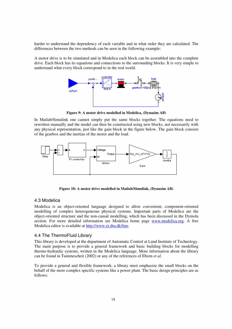
harder to understand the dependency of each variable and in what order they are calculated. Thedifferences between the two methods can be seen in the following example:

A motor drive is to be simulated and in Modelica each block can be assembled into the completedrive. Each block has its equations and connections to the surrounding blocks. It is very simple tounderstand what every block correspond to in the real world.

Figure 9: A motor drive modelled in Modelica, (Dynasim AB)

In Matlab/Simulink one cannot simply put the same blocks together. The equations need torewritten manually and the model can then be constructed using new blocks, not necessarily withany physical representation, just like the gain block in the figure below. The gain block consistsof the gearbox and the inertias of the motor and the load.

Figure 10: A motor drive modelled in Matlab/Simulink, (Dynasim AB)

4.3 ModelicaModelica is an object-oriented language designed to allow convenient, component-orientedmodelling of complex heterogeneous physical systems. Important parts of Modelica are theobject-oriented structure and the non-causal modelling, which has been discussed in the Dymolasection. For more detailed information see Modelica home page www.modelica.org. A freeModelica editor is available at http://www.et.dtu.dk/fme.

4.4 The ThermoFluid LibraryThis library is developed at the department of Automatic Control at Lund Institute of Technology.The main purpose is to provide a general framework and basic building blocks for modellingthermo-hydraulic systems, written in the Modelica language. More information about the librarycan be found in Tummescheit (2002) or any of the references of Eborn et al.

To provide a general and flexible framework, a library must emphasize the small blocks on thebehalf of the more complex specific systems like a power plant. The basic design principles are asfollows:

19

1. One unified library both for lumped and distributed parameter models,2. separation of the medium models, which can be selected through class parameters,3. both bi- and unidirectional flows are supported and4. assumptions (e.g. if gravity influence should be modelled) can be selected by the user

from user inputs.

The three major atomic parts of the library are:Control Volumes (CV) have a finite volume and are storages for mass and energy. The CV canbe either lumped or discretisised in space.Lumped Flow Models (FM) are the results of a modelling abstraction, where the volume isneglected, e.g. in valves and compressors. Algebraic equations relate variables, e.g. the pressuredrop and mass flow.Dynamic Flow Models (also abbreviated FM) can also calculate the storage of momentum in acontrol volume.

In combination with thermal models, dynamic flow models are only used when the focus is onvery fast transients like emergency shutdowns and the change of momentum is of importance.The lumped flow models are used, when the emphasis is on slow thermal applications, as e.g. thetemperature in heat exchangers. In the model of the T100 microturbine lumped flow models areused, since the main issue is normal power production and the corresponding thermal variables.

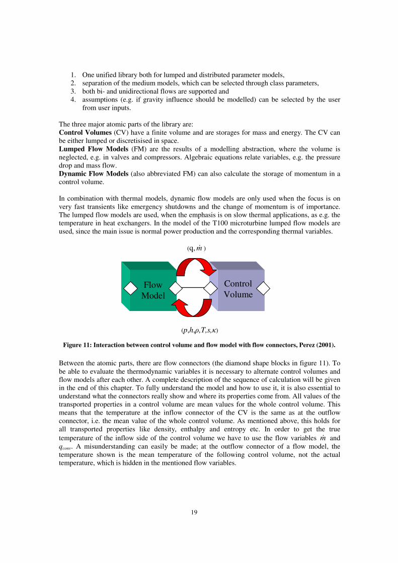
Between the atomic parts, there are flow connectors (the diamond shape blocks in figure 11). Tobe able to evaluate the thermodynamic variables it is necessary to alternate control volumes andflow models after each other. A complete description of the sequence of calculation will be givenin the end of this chapter. To fully understand the model and how to use it, it is also essential tounderstand what the connectors really show and where its properties come from. All values of thetransported properties in a control volume are mean values for the whole control volume. Thismeans that the temperature at the inflow connector of the CV is the same as at the outflowconnector, i.e. the mean value of the whole control volume. As mentioned above, this holds forall transported properties like density, enthalpy and entropy etc. In order to get the truetemperature of the inflow side of the control volume we have to use the flow variables m& andqconv. A misunderstanding can easily be made; at the outflow connector of a flow model, thetemperature shown is the mean temperature of the following control volume, not the actualtemperature, which is hidden in the mentioned flow variables.

Figure 11: Interaction between control volume and flow model with flow connectors, Perez (2001).

ControlVolume

(q, m& )

FlowModel

(p,h,ρ,T,s,κ)

20

(4.4.1)

(4.4.2)

(4.4.3)

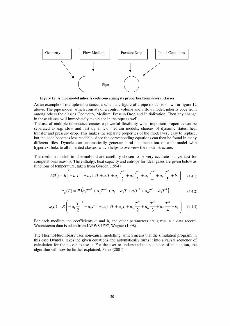
As an example of multiple inheritance, a schematic figure of a pipe model is shown in figure 12above. The pipe model, which consists of a control volume and a flow model, inherits code fromamong others the classes Geometry, Medium, PressureDrop and Initialization. Then any changein these classes will immediately take place in the pipe as well.The use of multiple inheritance creates a powerful flexibility when important properties can beseparated as e.g. slow and fast dynamics, medium models, choices of dynamic states, heattransfer and pressure drop. This makes the separate properties of the model very easy to replace,but the code becomes less readable, since the corresponding equations can then be found in manydifferent files. Dymola can automatically generate html-documentation of each model withhypertext links to all inherited classes, which helps to overview the model structure.

The medium models in ThermoFluid are carefully chosen to be very accurate but yet fast forcomputational reasons. The enthalpy, heat capacity and entropy for ideal gases are given below asfunctions of temperature, taken from Gordon (1994).

+++++++−= −

1

5

7

4

6

3

5

2

4321

1 5432ln)( b

Ta

Ta

Ta

TaTaTaTaRTh

( )47

36

2543

12

21)( TaTaTaTaaTaTaRTc p ++++++= −−

++++++−−= −

−

2

4

7

3

6

2

5431

2

2

1 432ln

2)( b

Ta

Ta

TaTaTaTa

TaRTs

For each medium the coefficients ai and bi and other parameters are given in a data record.Water/steam data is taken from IAPWS-IF97, Wagner (1998).

The ThermoFluid library uses non-causal modelling, which means that the simulation program, inthis case Dymola, takes the given equations and automatically turns it into a causal sequence ofcalculation for the solver to use it. For the user to understand the sequence of calculation, thealgorithm will now be further explained, Perez (2001).

Figure 12: A pipe model inherits code concerning its properties from several classes

Geometry Flow Medium Pressure Drop Initial Conditions

Pipe

21

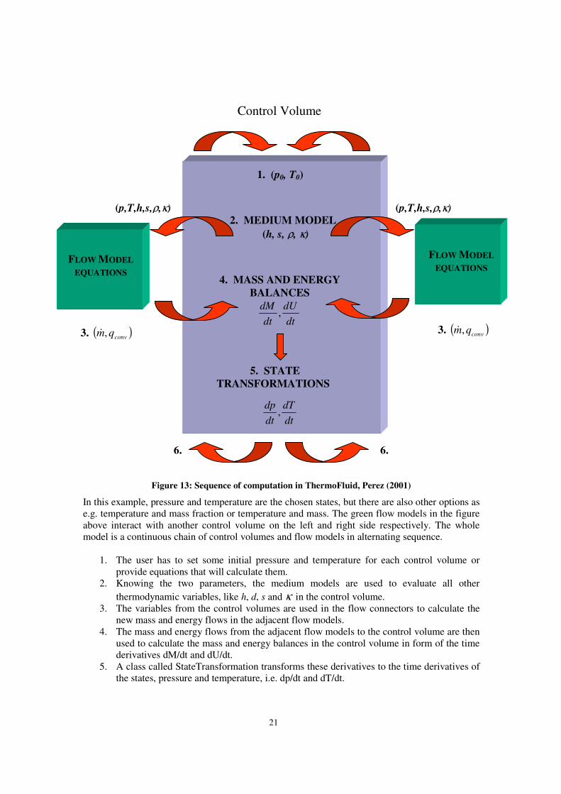
Figure 13: Sequence of computation in ThermoFluid, Perez (2001)

In this example, pressure and temperature are the chosen states, but there are also other options ase.g. temperature and mass fraction or temperature and mass. The green flow models in the figureabove interact with another control volume on the left and right side respectively. The wholemodel is a continuous chain of control volumes and flow models in alternating sequence.

1. The user has to set some initial pressure and temperature for each control volume orprovide equations that will calculate them.

2. Knowing the two parameters, the medium models are used to evaluate all otherthermodynamic variables, like h, d, s and κ in the control volume.

3. The variables from the control volumes are used in the flow connectors to calculate thenew mass and energy flows in the adjacent flow models.

4. The mass and energy flows from the adjacent flow models to the control volume are thenused to calculate the mass and energy balances in the control volume in form of the timederivatives dM/dt and dU/dt.

5. A class called StateTransformation transforms these derivatives to the time derivatives ofthe states, pressure and temperature, i.e. dp/dt and dT/dt.

3. ( )convqm,&

2. MEDIUM MODEL

1. (p0, T0)

4. MASS AND ENERGYBALANCES

5. STATETRANSFORMATIONS

(h, s, ρ, κ)

6.

(p,T,h,s,ρ,κ)

3. ( )convqm,&

FLOW MODEL

EQUATIONS

(p,T,h,s,ρ,κ)

FLOW MODEL

EQUATIONS

dt

dU

dt

dM,

dt

dT

dt

dp,

6.

Control Volume

22

(5.1.1)

(5.1.2)

(5.1.3)

(5.1.4)

6. Finally, these time derivatives are used to evaluate the new values of the states. Now thetemperature and pressure is once again known and the sequence returns to number 2.

5. Thermodynamic theory and modellingIn this chapter I will describe the individual components of a gas turbine, the thermodynamictheory of the components and how I have chosen to model them. The models of the compressor,turbine and combustion chamber are originally taken from Perez (2001) and have then beenmodified. Some of the following figures that describe vital parts of the microturbine, lack axesand are rescaled because of the classified information they contain.

5.1 The compressor equationsA centrifugal compressor is designed to increase the pressure of the gas using rotation. It usesmechanical work to rotate the rotor, thus accelerating the gas. After the rotor the gas passes adiffuser, where the increase in cross-section area gives a decrease in velocity and an increase inpressure, according to Bernoulli’s law. The total energy equation below can be found in Cengel(1998).

0=−−−− dpedkedhdwdqwhere dq is the specific external heating, dw is the specific net work, dh is the change in specificenthalpy, dke is the change in kinetic energy and dpe is the change in potential energy. Here theterm specific means the amount per unit mass. We can assume that the compressor is adiabatic(i.e. no heat flow in or out) so we can neglect the term dq. We do not have any height differencesso the same goes for the term dpe. The velocity does not change very much from the inlet of thecompressor to the exit of the diffuser. This small change in kinetic energy can therefore beneglected. This leaves us with:

dhdw =−The temperature and therefore the enthalpy increase at compression, resulting in dh as a positivenumber. The specific heat is defined as the energy required to raise the temperature of a unit massof a substance by one degree at constant pressure and can be written as:

pp T

hTc

∂∂=)(

After integrating over the compressor we get:

( )∫=−2

1dTTcw p

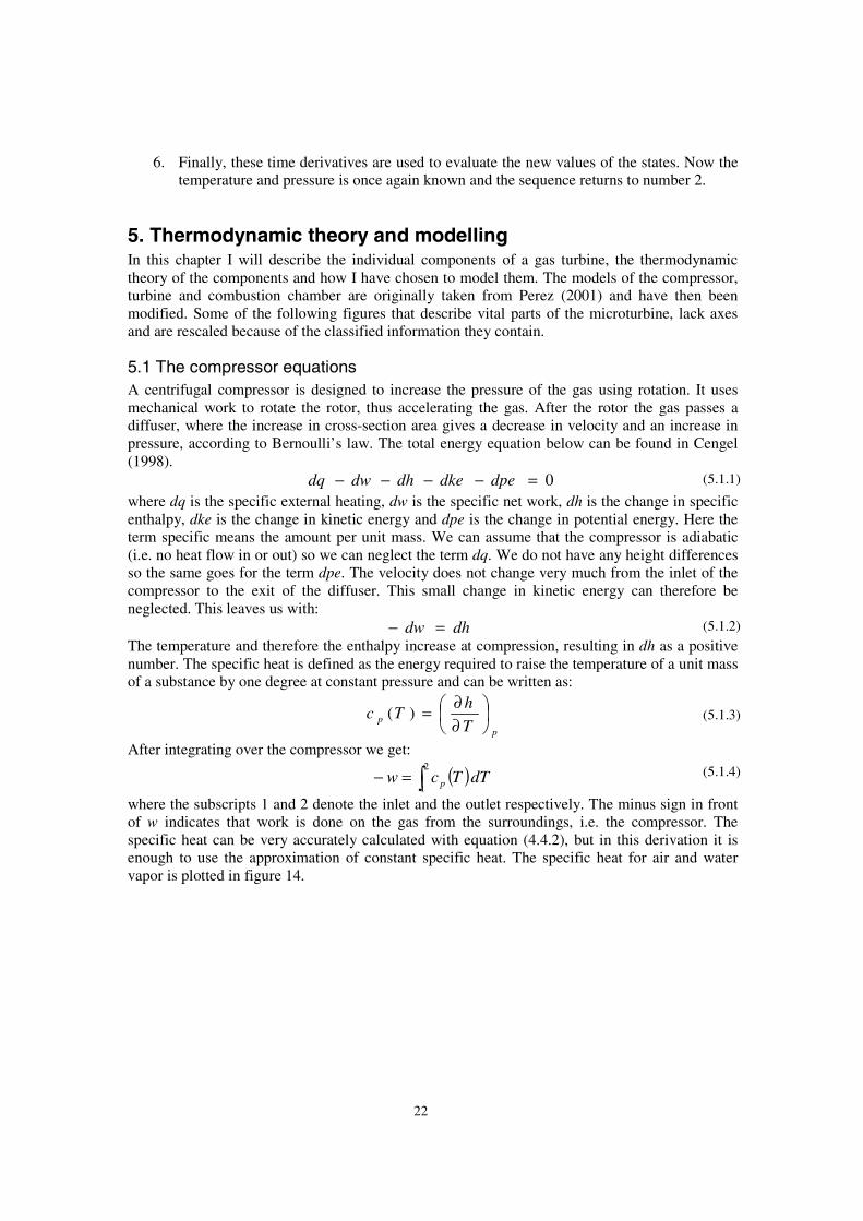
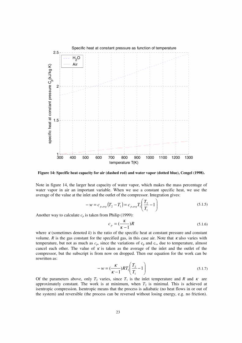
where the subscripts 1 and 2 denote the inlet and the outlet respectively. The minus sign in frontof w indicates that work is done on the gas from the surroundings, i.e. the compressor. Thespecific heat can be very accurately calculated with equation (4.4.2), but in this derivation it isenough to use the approximation of constant specific heat. The specific heat for air and watervapor is plotted in figure 14.

23

(5.1.5)

(5.1.6)

(5.1.7)

300 400 500 600 700 800 900 1000 1100 1200 13001

1.5

2

2.5

temperature T(K)

spec

ific

heat

at

cons

tant

pre

ssur

e C

p(kJ/

kg K

)Specific heat at constant pressure as function of temperature

H2O

Air

Figure 14: Specific heat capacity for air (dashed red) and water vapor (dotted blue), Cengel (1998).

Note in figure 14, the larger heat capacity of water vapor, which makes the mass percentage ofwater vapor in air an important variable. When we use a constant specific heat, we use theaverage of the value at the inlet and the outlet of the compressor. Integration gives:

( )

−=−=− 1

1

21,12, T

TTcTTcw avgpavgp

Another way to calculate cp is taken from Philip (1999):

Rc p )1

(−

=κ

κ

where κ (sometimes denoted k) is the ratio of the specific heat at constant pressure and constantvolume. R is the gas constant for the specified gas, in this case air. Note that κ also varies withtemperature, but not as much as cp, since the variations of cp and cv, due to temperature, almostcancel each other. The value of κ is taken as the average of the inlet and the outlet of thecompressor, but the subscript is from now on dropped. Then our equation for the work can berewritten as:

−

−=− 1)

1(

1

21 T

TRTw

κκ

Of the parameters above, only T2 varies, since T1 is the inlet temperature and R and κ areapproximately constant. The work is at minimum, when T2 is minimal. This is achieved atisentropic compression. Isentropic means that the process is adiabatic (no heat flows in or out ofthe system) and reversible (the process can be reversed without losing energy, e.g. no friction).

24

(5.1.8)

(5.1.9)

(5.1.10)

(5.1.11)

(5.1.12)

(5.1.13)

From Cengel (1998) we get the following expression for isentropic compression where thesubscript is denotes the variable at isentropic conditions:

κκ 1

1

2

1

,2

−

=

p

p

T

T is

The equation for the specific work can now be calculated using the inlet and outlet pressure andinput temperatures as follows:

−

−

=−

−

1)1

(

1

1

21

κκ

κκ

p

pRTwis

This is only valid for ideal processes, processes that are adiabatic and reversible. To compensatefor actual conditions, we use the thermodynamic variable, isentropic efficiency, defined as theratio of the enthalpy change at isentropic conditions and the actual enthalpy change:

( )( ) 12

1,2

12

1,2

12

1,2

TT

TT

TTc

TTc

hh

hh is

p

ispisis −

−=

−−

=−−

=η

The value of the isentropic efficiency can be determined through experiments, where thetemperatures are measured. Results from tests show that the efficiency does not however remainconstant for all pressure ratios. For increasing pressure ratios, there is a decrease in isentropicefficiency. A physical explanation is that the increase in temperature due to friction in one stageof the compression results in more work being required in the next stage, Cohen, (1996). Apartfrom friction, there is another factor that contributes to a lower efficiency. If another speed isused, different from the rotational speed the compressor is optimally designed for, this can causea difference in alignment with the gas flow and the impeller vanes. If the flow enters in an angledifferent from the angle of the impeller vanes, there will be small turbulent eddies right behindthe vanes and the efficiency of the compressor will decrease.

The actual specific work required can be formulated as:

isp

pRTw

ηκκ κ

κ 11)()

1(

1

1

21

−

−=−

−

The actual power needed to run the compressor is then simply:wmPcompressor ⋅= &

There can also be mechanical losses in the compressor. The compressor is mounted on a singleshaft and the relation between torque and power can be written as:

ωτη ⋅=⋅ compressormeccompressorP

where ω is the angular velocity of the shaft, τ is the torque the compressor consumes and ηmec isthe mechanical efficiency of the compressor.

5.2 The compressor model in ModelicaBased on the equations derived above a model of the compressor was developed. The model istaken from Perez (2001) and then modified.

There are some properties that cannot be calculated analytically, e.g. the isentropic efficiency andthe mass flow through the compressor. These must instead come from empirical data, which isgiven in the form of a compressor map. In the map, the mass flow and efficiency are given asfunctions of other known variables, usually the speed and the pressure ratio. The compressor map

25

(5.2.1)

(5.2.2)

(5.2.3)

can be generated either by physical experiments or very detailed calculations. In the case of theT100, the computations were carried out at Volvo Aero Corporation (VAC) AB.

The map is generated from a steady state situation for a certain temperature, pressure and speed.In order for the map to clearer present its data, a usual trick is to reduce the number ofparameters, by using non-dimensional analysis. This is done in the form of the non-dimensionalvariables, corrected speed and corrected mass flow. The variables are normalized with theambient temperature and pressure during the experiment/calculation. For more background onnon-dimensional analysis see Fox (1998) and Cohen (1996). The corrected speed and mass flowshould also include the diameter D and the gas constant R in order to be dimensionless, but thesevariables are constant for the compressor, thus they can be neglected.

We define:

Pressure ratio1

2

p

ppr =

Corrected mass flow1

1

p

Tmmcorr

&& =

Corrected speed1T

nncorr =

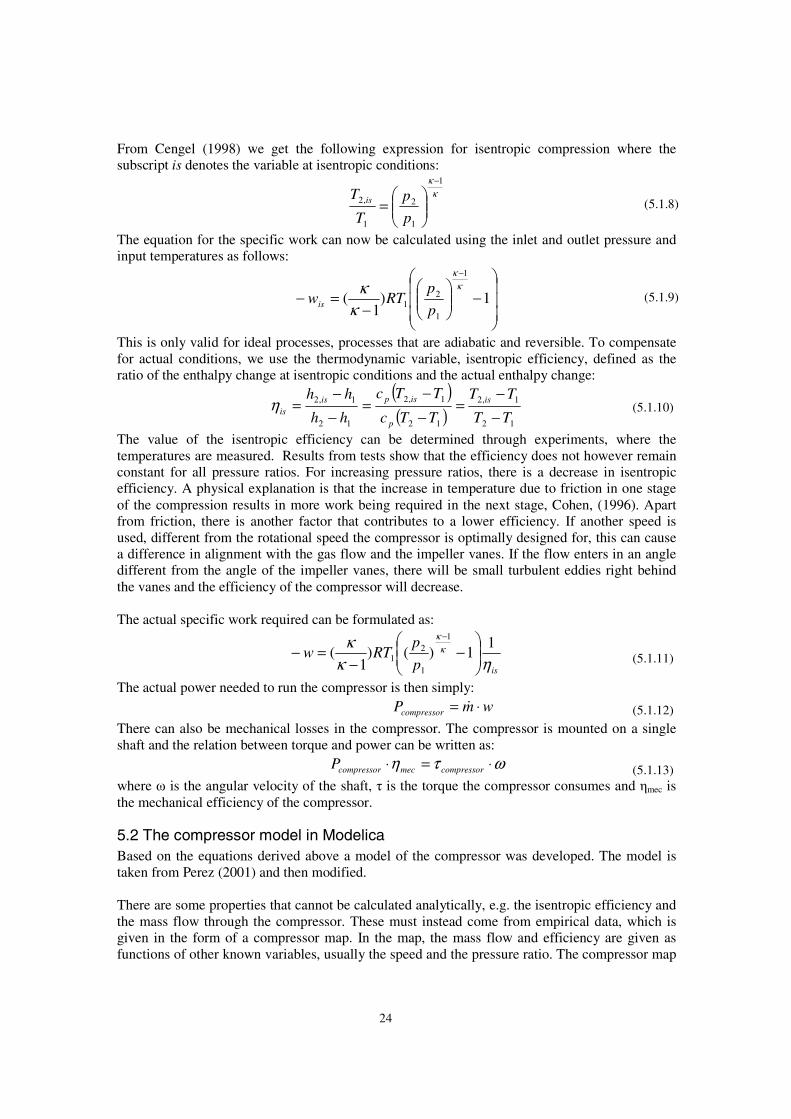
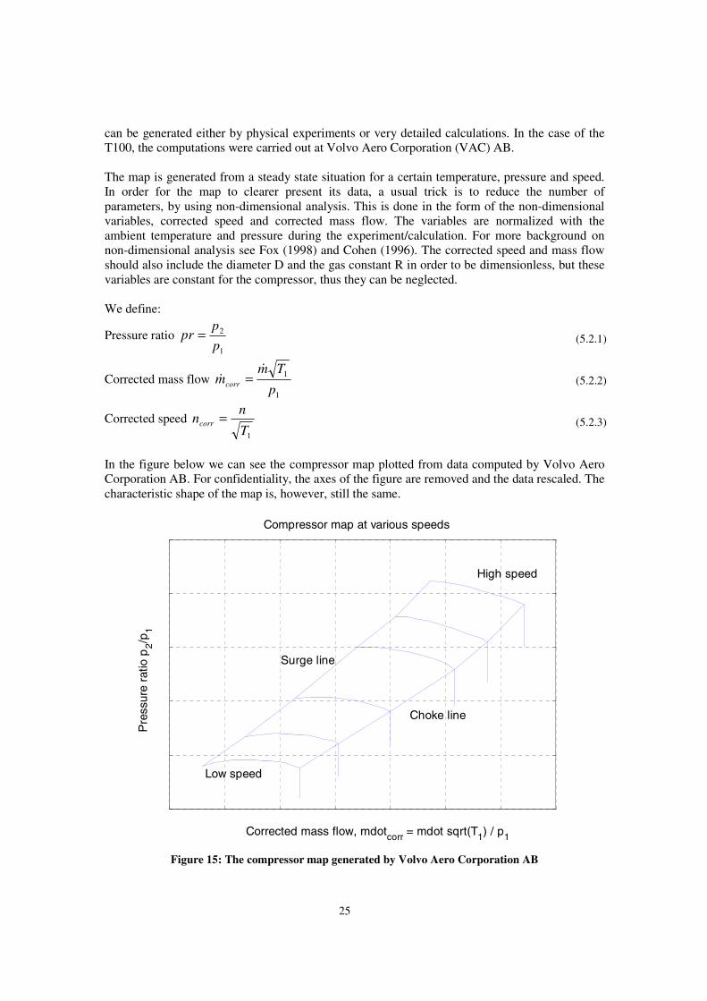
In the figure below we can see the compressor map plotted from data computed by Volvo AeroCorporation AB. For confidentiality, the axes of the figure are removed and the data rescaled. Thecharacteristic shape of the map is, however, still the same.

Compressor map at various speeds

Pre

ssur

e ra

tio p

2/p

1

Surge line

Low speed

Choke line

High speed

Corrected mass flow, mdotcorr = mdot sqrt(T1) / p1

Figure 15: The compressor map generated by Volvo Aero Corporation AB

26

(5.2.4)

Each of the horizontal curves corresponds to one constant speed of rotation. The range is from 20000 rpm up to 74 000 rpm. The area enclosed by the surge line and the choke line is the normaloperating range for the compressor. On the left side of the surge line the pressure ratio decreasesfor decreasing mass flow, i.e. a positive pressure gradient. This can, for the lower speeds, alreadybe seen on the immediate right side of the surge line. Surge is associated with a drop in thepressure ratio, i.e. the delivery pressure, which can lead to pulsations in the mass flow and evenreverse it. It can cause considerable damage to the compressor, e.g. blade failure. The surgephenomenon is similar to wing stall of an airplane. Rotating stall is another dangerous event.It occurs when cells of separated flow form and block a segment of the compressor rotor.Performance is decreased and the rotor might be unbalanced, also leading to failures, Fox (1998).

As the pressure ratio decreases and mass flow increases, the radial velocity of the flow must alsoincrease, in order for the compressor to blow enough gas through it. At some point thecompressor cannot accelerate the flow to high enough radial velocity for the given motor speed,then maximum mass flow is reached and choking is said to occur, Cohen (1996).

The compressor map model must in one way or another represent the theoretical compressor map.One obvious method is taking the raw tables of data that produce the curves above and use themin a look-up table. Between data points bilinear interpolation can be used. This method was testedin the compressor model for the mass flow and the efficiency. Unfortunately it did not work, dueto numerical problems, which will be discussed in the end of the compressor section.

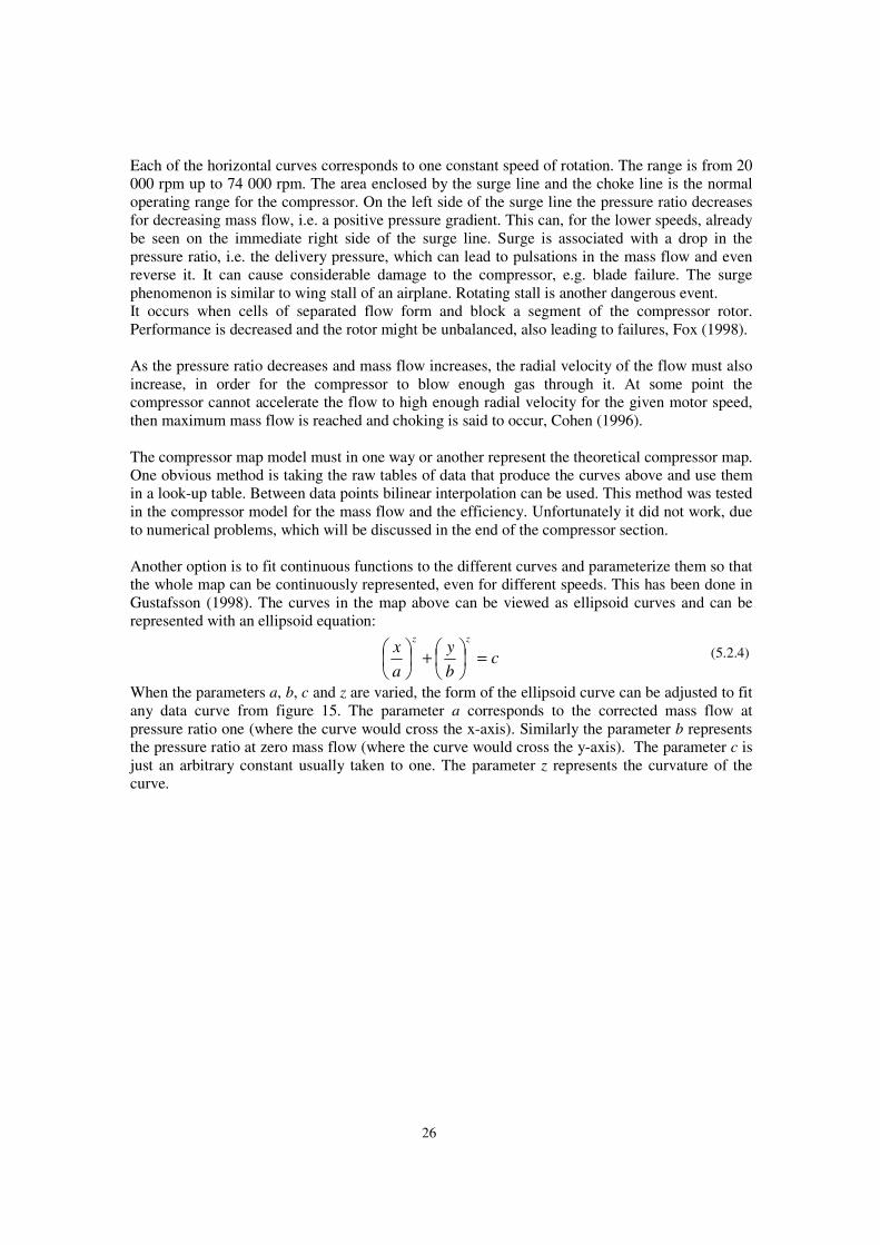
Another option is to fit continuous functions to the different curves and parameterize them so thatthe whole map can be continuously represented, even for different speeds. This has been done inGustafsson (1998). The curves in the map above can be viewed as ellipsoid curves and can berepresented with an ellipsoid equation:

cb

y

a

xzz

=

+

When the parameters a, b, c and z are varied, the form of the ellipsoid curve can be adjusted to fitany data curve from figure 15. The parameter a corresponds to the corrected mass flow atpressure ratio one (where the curve would cross the x-axis). Similarly the parameter b representsthe pressure ratio at zero mass flow (where the curve would cross the y-axis). The parameter c isjust an arbitrary constant usually taken to one. The parameter z represents the curvature of thecurve.

27

(5.2.5)

corrected mass flow, mdotcorr=mdot sqrt(T1)/p1

pres

sure

rat

io,

p2/p

1

A single ellipsoid curve and the surge line

a

b

surge line

(x,y)

Figure 16: An ellipsoid curve based on equation (5.2.4)

The values of the a parameters are first taken from the compressor map and the parameter z is atfirst parameterized with a linear increase with speed, as done in Perez (2001). To get the bparameter we use the ellipsoid equation with a known input, the point (x, y) from the map, wherethe curve crosses the surge line. With the values of x and y we can calculate b. Now the ellipsoidcurve is matched with the given data at least in one point. Unfortunately the values of a and z arenot good enough to give accurate results all along the curve. Instead manually adjustments aremade to the parameters a and z for each speed to minimize (via visual inspection) the deviationsbetween the ellipsoid curves and data from the map. There is no need for the ellipsoid curves tofit outside the actual operating range; instead emphasis is put on matching the data as good aspossible within the operating range. As can be seen in figure 17 below, the model curves differ alot from the data outside this range. Now each speed from the map is modelled by equation(5.2.4), uniquely determined by its parameters a, b, c and z.

In order to generate a continuous mapping for all possible speeds, a polynomial function is fittedfor each parameter a, b and z. The calculations were done in Matlab using the polyfitcommand. The polynomials are of an order between 4 and 7, depending on the nature of the data.With the polynomials, the parameters can during the simulation be evaluated for a continuous setof speeds from 21 000 rpm to 74 000 rpm like this:

pa(5)ncorrpa(4)ncorrpa(3)ncorrpa(2)+ncorrpa(1) 234 +⋅+⋅+⋅⋅=a

where pa is a vector containing the polynomial coefficients from the polyfit function andncorr is the corrected speed. The other parameters b and z are evaluated in the same manner.

28

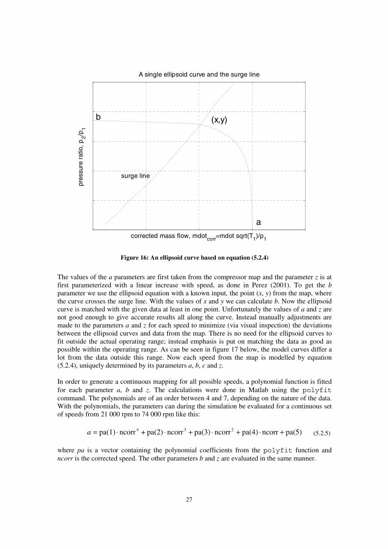
Given a known pressure ratio and speed we want to know the corresponding mass flow. In theoriginal map this might be a problem since the curves for the lower speeds are not monotonic, i.e.there is no unique solution to the problem. With the use of elliptic curves we get monotonic yetaccurate functions. An obvious drawback with the method is the large manual part of the functionfitting. It makes the process less automatic, when new compressors are introduced, but on theother hand it gives a model that works for the whole operating range. The errors introduced comefirstly from the curve fitting procedure, and secondly, new errors arise when the curves areparameterized with speed. The error of the mass flow model is around 2.9 %, around the normaloperating point of 70 000 rpm, see the result section, and is in general somewhat higher for lowerspeeds. Especially when the gas turbine operates near the surge line where the model curve isalmost flat; a small error in the pressure ratio gives a larger error in the mass flow. However thegas turbine operates only in the lower regions during the start up or stop procedure and then thefunctionality of the model is emphasized over absolute accuracy.The surge points and choke points for each speed are gathered and parameterized with speed.During simulation these polynomial functions are evaluated with the current speed to get anestimate of how close the current operating point is to the surge and choke line.

Compressor map and model curves, at various speeds

Corrected mass flow, mdotcorr = mdot sqrt(T1) / p1

Pre

ssur

e ra

tio,

p2/p

1

Surge line

Choke line

Low speed

High speed

Figure 17: Compressor map (solid blue) and fitted ellipsoid curves (dashed red)

Summary of the development of the mass flow model of the compressor:1. The value of the parameter a is taken from the map, i.e. the mass flow value at choking

conditions.2. The parameter z is set to an arbitrarily value, e.g. 5.3. One data point (x, y) is taken from the map, where the ellipsoid curve and data will be

identical matched. Using this point, equation (5.2.4) is solved for the parameter b.4. The curve is plotted and compared to data from the map. By visual inspection, the

parameters a and z are modified to ensure a better fit inside the operating range.

29

(5.2.6)

5. For each speed there is a different set of parameters. The values of the parameters arenow parameterized with speed in Matlab to polynomial functions to achieve a continuousmodel.

6. With the complete model, the mass flow is now continuously given by speed andpressure ratio.

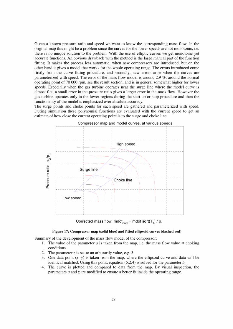
Modelling the isentropic efficiency was harder. As can be seen in the figure below, there is noellipsoid form to use. For a given rotational speed, the maximum efficiency is well-known, i.e.the top value of the curve. Knowing the maximum efficiency, we can approximate the efficiencymap with parabolic degradation curves. The amount of curvature or degradation is denoted d andis fitted based on numerous data to get parameterization for all speeds. The following equation istaken from Gustafsson (1998).

( ) 2maxmax effmmd && −−= ηη

Corrected mass flow, mdotcorr=mdot sqrt(T1)/p1

Isen

trop

ic e

ffic

ienc

y

Compressor efficiency from map and model at various speeds

63 000 rpm

66 500 rpm

70 000 rpm

Figure 18: Isentropic efficiency from map (solid blue) and model (dashed red) as a function of speedand mass flow

As can be seen in the figure above, the curves are not exactly symmetrical. Near chokingconditions (to the right), the performance is decreased rapidly. Another difficult part in this caseis that the curvature changes a factor of 20 from the lowest to the highest speed. It is hard tocreate a continuous function that gives the correct value at every speed. Instead a simpleinterpolation function was used. At steady state the microturbine is very close to optimum, wherethe model is very accurate. At the extreme ends of the operating range, as e.g. near surge andchoking, the accuracy decreases, due to errors both in the modelled mass flow and modelledefficiency.

So why did the interpolation method not work for the compressor mass flow or efficiency? Thefirst obvious drawback is that for lower speeds the map does not have a unique solution for agiven pressure and speed. As we did for the continuous ellipsoid curves we can manually change

30

the pressure curves such that we have a monotonic map. A more important drawback is that thederivative of the mass flow would not be continuous with a bilinear interpolation. This can lead tonumerical problems in the simulation. For some parameters like mass flow and pressure it isessential to have the derivative continuous, in order to do physically correct modelling. There areother interpolation methods, e.g. using cubic splines to generate continuous maps. The drawbackhere is then that we need to calculate 16 spline coefficients for each grid point in the interpolationmap. In our case with 176 grid points and four interpolation tables we would need to calculate11264 coefficients. Doing good modelling with interpolation methods is not an easy subject andis beyond the scope of this thesis.

The bilinear interpolation method was tested for the compressor mass flow and efficiency, butcould not prove to be reliable in the whole operating range, even after the compressor map hadbeen manually altered to provide unique solutions for lower speeds. In most cases the simulationwas halted or got stuck due to chattering (discontinuity sticking). What happens is that a variable,e.g. speed is changed causing the interpolation index of the axis of the interpolation table to alsochange. The interpolated output data, e.g. the mass flow, causes the speed to change back andthen the index is changed back as well and so on and so forth. This might be partly caused by thefact that the data is not rectangular. With this means that each speed has a different pressure ratiointerval, e.g. for 20 000 rpm the pressure ratio ranges from 1.18 to 1.02, whereas for 70 000 rpmthe pressure ratio ranges from 5.2 to 4.8. This means that e.g. index 1 (the first vertical column)represents different pressure ratios depending on speed. The turbine data, however, is inrectangular form. All the speeds have the same range of pressure ratio and e.g. the index 1 (thefirst vertical column) always represent data at a pressure ratio of 1.25. The reasons behind this aresimple. The compressor compresses the air and can for a certain speed only create a certainmaximum pressure ratio. The higher the speed the higher is the pressure ratio created. The turbineexpands the gas and work for all different pressure ratios and speeds, since it uses the pressureratio created by the compressor. Another problem is when the numerical solver of the n:th orderexpects to find equations that are n times differentiable and the equations are only differentiableof a lower order. Often the solver succeeds despite this, but there are always reasons to be careful.

The mechanical efficiency of the compressor is taken to 100 %, since the major friction losses inthe microturbine come from the two bearings, which are modelled in a separate submodel, seesection 5.10.

5.3 The turbine equationsBefore the exhaust gas enters the turbine, it passes through a nozzle where the velocity isincreased and the pressure decreases. The high-speed gas exerts a force on the turbine blades andthe geometry of the blade causes the turbine to rotate, thus producing mechanical work. After theturbine rotor, the gas passes through the diffuser of the turbine, where again the velocity isdecreased and the pressure increased but not as much as after the compressor.The thermodynamic equations are in large parts the same as for the compressor. Instead ofrepeating all of the derivations, there will be references to the corresponding compressor section.

We have the same energy balance as we used for the compressor. Also the same approximationscan be made about the turbine. The only difference is that work is now done by the gas on thesurroundings, i.e. on the turbine. The equation for the isentropic work of the turbine is thereforeexactly as equation (5.1.9) but with the sign changed.

From equation (5.1.8) we get the relation for isentropic expansion and by including the isentropicefficiency from equation (5.1.10), the equation for the produced actual work can be rewritten as:

31

(5.3.1)

(5.3.2)

(5.3.3)

−

−=

−κ

κ

κκη

1

1

21 )(1)

1(

p

pRTw is

For increasing pressure ratios, an increase in isentropic efficiency of the turbine can be seen. Aphysical explanation is that the increase in temperature due to friction in one part of the expansioncan be recovered as work on the turbine in the next part, Cohen (1996).

The produced power from the turbine is then:

−

−⋅=

−κ

κ

κκη

1

1

21 )(1)

1(

p

pRTmP isturbine &

The turbine is mounted on the same shaft as the compressor, producing enough torque to powerthe compressor and the generator. Similar to the compressor, the turbine has a mechanicalefficiency, depending on design and construction. The relation between the mechanical torqueand the power produced can be written as:

ωτη ⋅=⋅ turbinemecturbineP

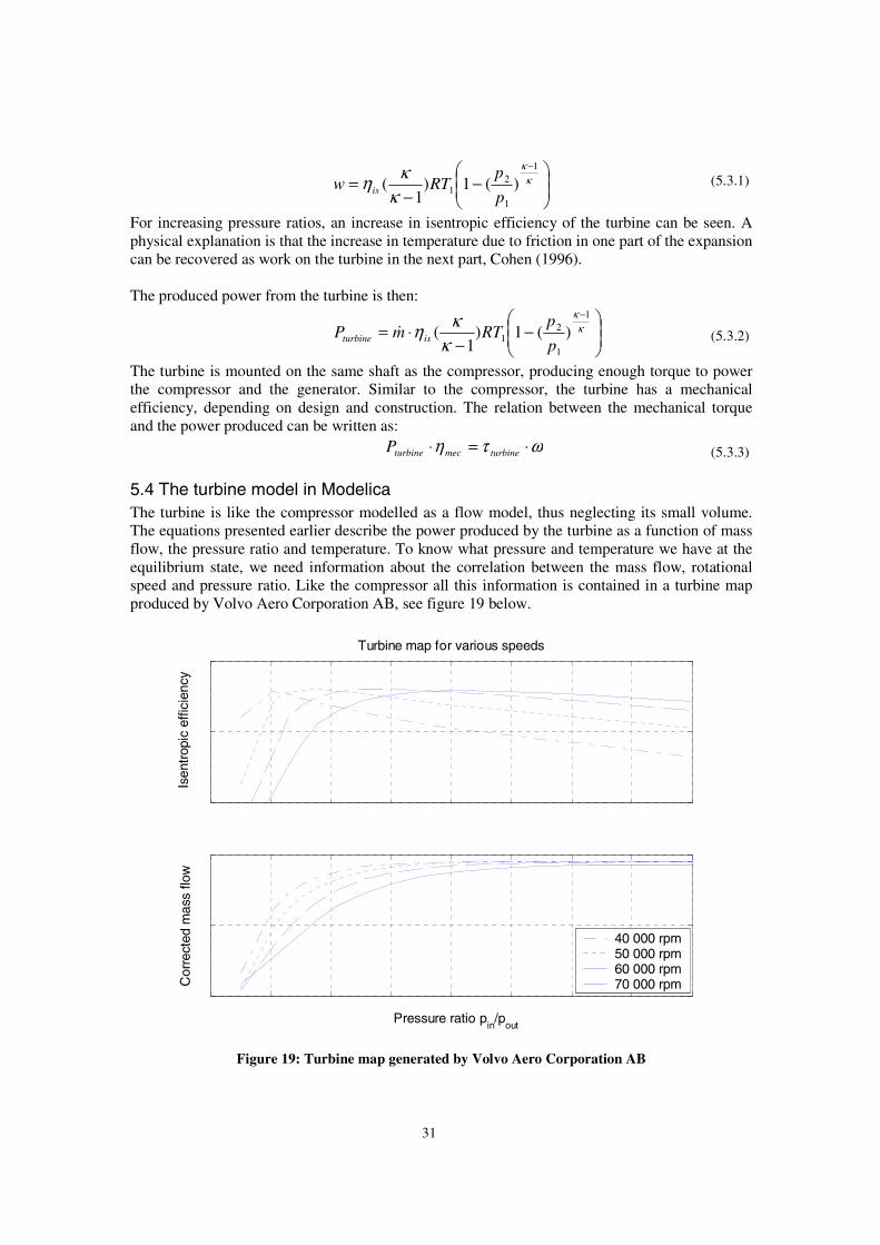
5.4 The turbine model in ModelicaThe turbine is like the compressor modelled as a flow model, thus neglecting its small volume.The equations presented earlier describe the power produced by the turbine as a function of massflow, the pressure ratio and temperature. To know what pressure and temperature we have at theequilibrium state, we need information about the correlation between the mass flow, rotationalspeed and pressure ratio. Like the compressor all this information is contained in a turbine mapproduced by Volvo Aero Corporation AB, see figure 19 below.

Isen

trop

ic e

ffici

ency

Turbine map for various speeds

pressure ratio pin/p

out

Pressure ratio pin/p

out

Cor

rect

ed m

ass

flow

40 000 rpm50 000 rpm60 000 rpm70 000 rpm

Figure 19: Turbine map generated by Volvo Aero Corporation AB

32

(5.4.1)

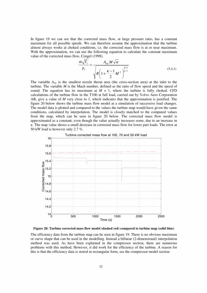
In figure 19 we can see that the corrected mass flow, at large pressure ratio, has a constantmaximum for all possible speeds. We can therefore assume the approximation that the turbinealmost always works at choked conditions, i.e. the corrected mass flow is at or near maximum.With the approximation, we can use the following equation to calculate the constant maximumvalue of the corrected mass flow, Cengel (1998).

1

1

21

1

2

11

−+

−+

=κκ

κ

κ

MR

MA

p

Tmthr

&

The variable Athr is the smallest nozzle throat area (the cross-section area) at the inlet to theturbine. The variable M is the Mach number, defined as the ratio of flow speed and the speed ofsound. The equation has its maximum at M = 1, where the turbine is fully choked. CFDcalculations of the turbine flow in the T100 at full load, carried out by Volvo Aero CorporationAB, give a value of M very close to 1, which indicates that the approximation is justified. Thefigure 20 below shows the turbine mass flow model at a simulation of successive load changes.The model data is plotted and compared to the values the turbine map would have given the sameconditions, calculated by interpolation. The model is closely matched to the computed valuesfrom the map, which can be seen in figure 20 below. The corrected mass flow model isapproximated as a constant, even though the value actually increases some, due to an increase inκ. The map value shows a small decrease in corrected mass flow for lower part loads. The error at50 kW load is however only 2.7 %.

0 500 1000 1500 2000 250014

14.2

14.4

14.6

14.8

15

15.2

15.4

15.6

15.8

16Turbine corrected mass flow at 100, 70 and 50 kW load

Time (s)

Cor

rect

ed m

ass

flow

Figure 20: Turbine corrected mass flow model (dashed red) compared to turbine map (solid blue)

The efficiency data from the turbine map can be seen in figure 19. There is no obvious maximumor curve shape that can be used in the modelling. Instead a bilinear (2-dimensional) interpolationmethod was used. As have been explained in the compressor section, there are numerousproblems with this method. However, it did work for the efficiency of the turbine. A reason forthis is that the efficiency data is stored in rectangular form, see the compressor model section

33

(5.4.2)

(5.4.3)

(5.4.4)

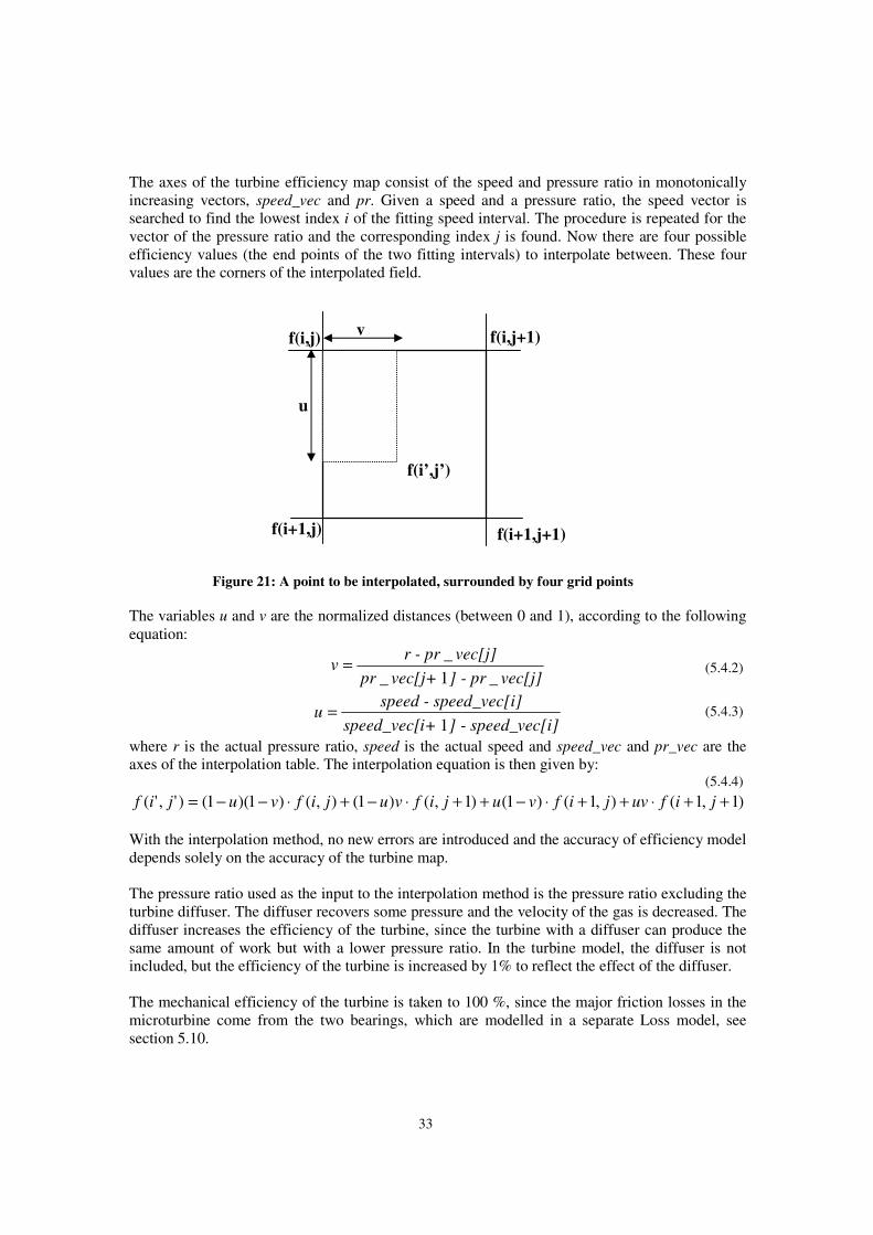
The axes of the turbine efficiency map consist of the speed and pressure ratio in monotonicallyincreasing vectors, speed_vec and pr. Given a speed and a pressure ratio, the speed vector issearched to find the lowest index i of the fitting speed interval. The procedure is repeated for thevector of the pressure ratio and the corresponding index j is found. Now there are four possibleefficiency values (the end points of the two fitting intervals) to interpolate between. These fourvalues are the corners of the interpolated field.

The variables u and v are the normalized distances (between 0 and 1), according to the followingequation:

vec[j]] - prvec[j+pr

vec[j]r - prv

_1_

_=

vec[i]] - speed_i+speed_vec[

eed_vec[i]speed - spu

1=

where r is the actual pressure ratio, speed is the actual speed and speed_vec and pr_vec are theaxes of the interpolation table. The interpolation equation is then given by:

)1,1(),1()1()1,()1(),()1)(1()','( ++⋅++⋅−++⋅−+⋅−−= jifuvjifvujifvujifvujif

With the interpolation method, no new errors are introduced and the accuracy of efficiency modeldepends solely on the accuracy of the turbine map.

The pressure ratio used as the input to the interpolation method is the pressure ratio excluding theturbine diffuser. The diffuser recovers some pressure and the velocity of the gas is decreased. Thediffuser increases the efficiency of the turbine, since the turbine with a diffuser can produce thesame amount of work but with a lower pressure ratio. In the turbine model, the diffuser is notincluded, but the efficiency of the turbine is increased by 1% to reflect the effect of the diffuser.

The mechanical efficiency of the turbine is taken to 100 %, since the major friction losses in themicroturbine come from the two bearings, which are modelled in a separate Loss model, seesection 5.10.

f(i,j) f(i,j+1)

f(i+1,j) f(i+1,j+1)

f(i’,j’)

u

v

Figure 21: A point to be interpolated, surrounded by four grid points

34

5.5 The heat exchangerThe function of a heat exchanger is to transfer heat from one medium to another, often separatedby a solid wall. It can be used in space heating, air-conditioning, power production and chemicalprocessing. The following information and more can be found in DeWitt (1996) and Gustafsson(1998). There are different heat exchangers depending on flow arrangement and type ofconstruction. The simplest heat exchanger is a concentric tube where the fluids flow in eitherparallel direction or in a counterflow manner. Another version is the crossflow heat exchangerwhere the fluids meet perpendicular to each other.

There are numerous methods of analysis, the two most common are the log-mean temperaturedifference and the effectiveness (efficiency) -NTU method. The log-mean method is used whenthe outlet temperatures are given by specifications or can be readily determined from the energybalances. It is also used in heat exchangers with low order of discretisation. In other cases theeffectiveness-NTU method is to be preferred. The outlet temperatures are unknown in the T100and therefore only the effectiveness-NTU method will be described.

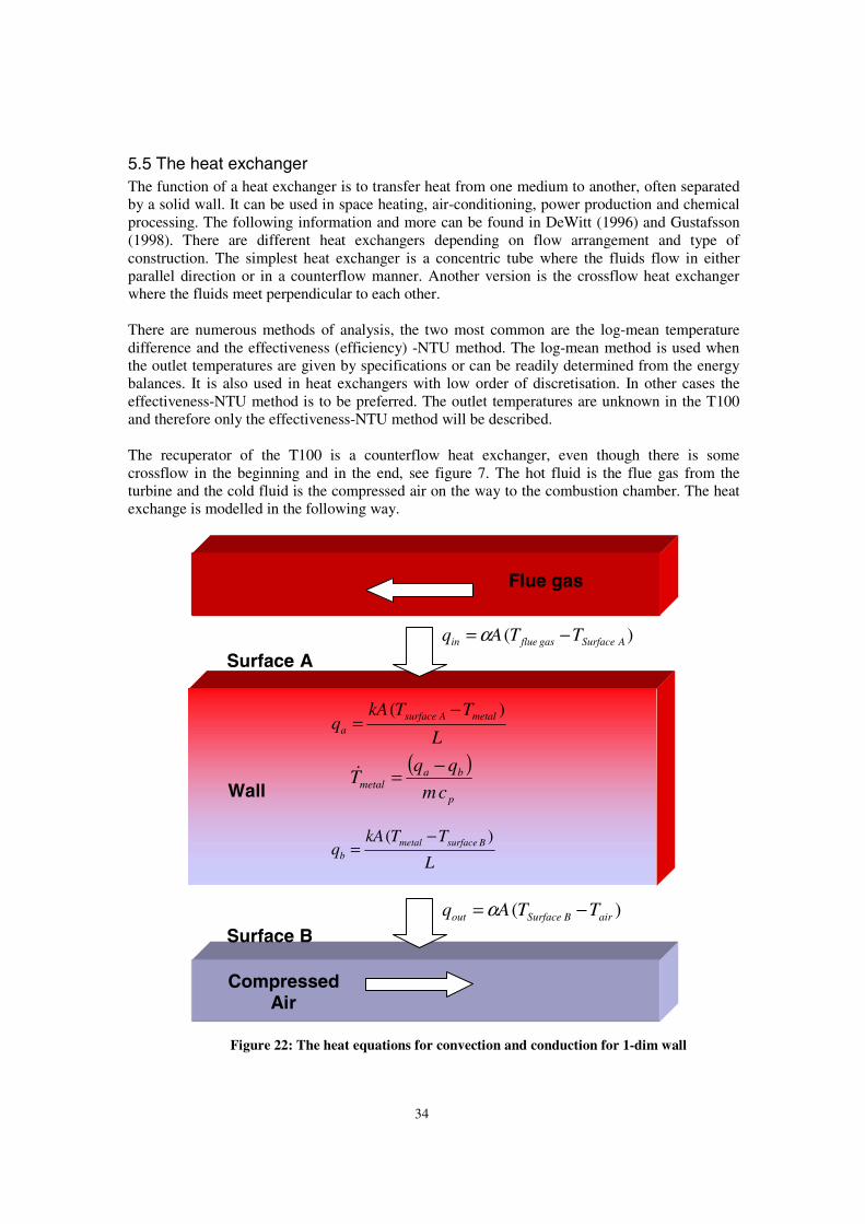
The recuperator of the T100 is a counterflow heat exchanger, even though there is somecrossflow in the beginning and in the end, see figure 7. The hot fluid is the flue gas from theturbine and the cold fluid is the compressed air on the way to the combustion chamber. The heatexchange is modelled in the following way.

Wall

Flue gas

Surface A

CompressedAir

Surface B

)( ASurfacegasfluein TTAq −= α

L

TTkAq metalAsurface

a

)( −=

)( airBSurfaceout TTAq −= α

( )p

bametal cm

qqT

−=&

L

TTkAq Bsurfacemetal

b

)( −=

Figure 22: The heat equations for convection and conduction for 1-dim wall

35

(5.5.1)

(5.5.2)

(5.5.3)

(5.5.4)

(5.5.5)

(5.5.6)

(5.5.7)

where α is the convection heat transfer coefficient, k is the conduction heat transfer coefficient, Lis the thickness of the wall, m is the mass of the wall and cp is the specific heat of the metal in thewall. These equations describe the dynamics of the temperature in the wall. The heat transfer isapproximated to the 1-dimensional case, but since the wall is very thin compared to the length, itis a justified approximation.We also want to define the efficiency of a heat exchanger, so that we know how good it iscompared to an ideal heat exchanger. In order to do so we start by defining the maximum possibleheat transfer rate:

)( ,,min inairingasflue TTCq −=where

})(,)min{(min gasfluepairp mcmcC &&=Cmin is minimum heat capacity flow of the two involved fluids. The subscripts in and out refer tothe inlet and outlet of the heat exchanger and the subscript air and flue gas refer to the cold andhot fluid of the heat exchanger respectively. The maximum heat transfer can only be achieved inan ideal counterflow heat exchanger of infinite length. The actual heat transfer can thus be statedas:

)( ,, inairoutairair TTCq −=which gives us a formal definition on the efficiency:

inairingasflue

inairoutair

inairingasflue

inairoutairair

TT

TT

TTC

TTC

q

q

,,

,,

,,min

,,

max )(

)(

−−

=−

−==ε

In the T100 microturbine, the fluids are air and flue gas. The only differences between thesubstances are somewhat lower percentage oxygen and higher percentage carbon dioxide andwater vapor. When the fuel is added, the total mass flow is increased, but only with 1 % due tothe large air/fuel ratio. The exhaust gas has also higher temperature than the air, which also givesa little larger cp. Then Cmin = Cair and we get the right had side of equation (5.5.4).

The equation above gives the efficiency of the heat exchanger based on temperaturemeasurements. It is used to evaluate the efficiency of a recuperator in use. It does not, however,say anything in advance about what the efficiency a designed recuperator will have and whatfactors that can improve the efficiency. Another useful expression for the efficiency is thereforetaken from DeWitt (1996). The following equation is only valid when the heat capacity flows ofthe fluids are equal, which is a justified approximation in the case of the T100 microturbine.

NTU

NTU

+=

1ε

The variable NTU (number of thermal units) is a dimensionless parameter that is widely used forheat exchangers. It shows how well the heat exchanger can transfer heat due to its geometry, massflow, mediums and heat transfer coefficients.

minC

AUNTU

⋅=

where A is the heat exchanger surface area and U [W/m2 K] is the overall heat transfer coefficientdefined as

)11

(

1

fluegaswallair k

LU

αα++

=

The variable α is the convection heat transfer coefficient; L is the thickness of the wall and k isthe thermal conductivity (conduction heat transfer coefficient). The wall between the fluids is

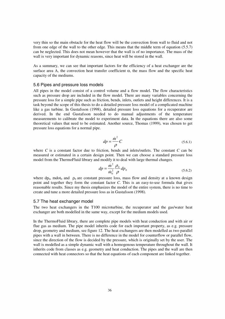
36

(5.6.1)

(5.6.2)

very thin so the main obstacle for the heat flow will be the convection from wall to fluid and notfrom one edge of the wall to the other edge. This means that the middle term of equation (5.5.7)can be neglected. This does not mean however that the wall is of no importance. The mass of thewall is very important for dynamic reasons, since heat will be stored in the wall.

As a summary, we can see that important factors for the efficiency of a heat exchanger are thesurface area A, the convection heat transfer coefficient α, the mass flow and the specific heatcapacity of the mediums.

5.6 Pipes and pressure loss modelsAll pipes in the model consist of a control volume and a flow model. The flow characteristicssuch as pressure drop are included in the flow model. There are many variables concerning thepressure loss for a simple pipe such as friction, bends, inlets, outlets and height differences. It is atask beyond the scope of this thesis to do a detailed pressure loss model of a complicated machinelike a gas turbine. In Gustafsson (1998), detailed pressure loss equations for a recuperator arederived. In the end Gustafsson needed to do manual adjustments of the temperaturemeasurements to calibrate the model to experiment data. In the equations there are also sometheoretical values that need to be estimated. Another source, Thomas (1999), was chosen to getpressure loss equations for a normal pipe.

Cm

dpρ

2&=

where C is a constant factor due to friction, bends and inlets/outlets. The constant C can bemeasured or estimated in a certain design point. Then we can choose a standard pressure lossmodel from the ThermoFluid library and modify it to deal with large thermal changes.

00

20

2

dpm

mdp

ρρ

&

&=

where dp0, mdot0 and ρ0 are constant pressure loss, mass flow and density at a known designpoint and together they form the constant factor C. This is an easy-to-use formula that givesreasonable results. Since my thesis emphasizes the model of the entire system, there is no time tocreate and tune a more detailed pressure loss as in Gustafsson (1998).

5.7 The heat exchanger modelThe two heat exchangers in the T100 microturbine, the recuperator and the gas/water heatexchanger are both modelled in the same way, except for the medium models used.

In the ThermoFluid library, there are complete pipe models with heat conduction and with air orflue gas as medium. The pipe model inherits code for each important property, as e.g. pressuredrop, geometry and medium, see figure 12. The heat exchangers are then modelled as two parallelpipes with a wall in between. There is no difference in the model for counterflow or parallel flow,since the direction of the flow is decided by the pressure, which is originally set by the user. Thewall is modelled as a simple dynamic wall with a homogenous temperature throughout the wall. Itinherits code from classes as e.g. geometry and heat conduction. The pipes and the wall are thenconnected with heat connectors so that the heat equations of each component are linked together.

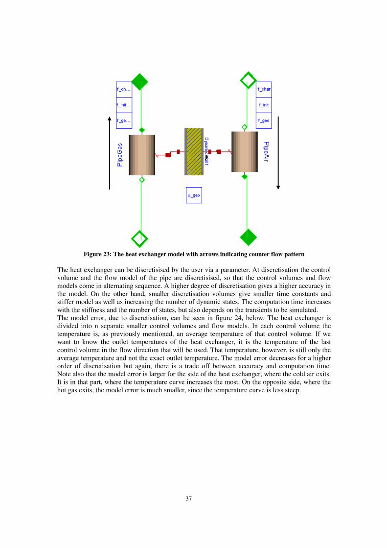
37

Figure 23: The heat exchanger model with arrows indicating counter flow pattern

The heat exchanger can be discretisised by the user via a parameter. At discretisation the controlvolume and the flow model of the pipe are discretisised, so that the control volumes and flowmodels come in alternating sequence. A higher degree of discretisation gives a higher accuracy inthe model. On the other hand, smaller discretisation volumes give smaller time constants andstiffer model as well as increasing the number of dynamic states. The computation time increaseswith the stiffness and the number of states, but also depends on the transients to be simulated.The model error, due to discretisation, can be seen in figure 24, below. The heat exchanger isdivided into n separate smaller control volumes and flow models. In each control volume thetemperature is, as previously mentioned, an average temperature of that control volume. If wewant to know the outlet temperatures of the heat exchanger, it is the temperature of the lastcontrol volume in the flow direction that will be used. That temperature, however, is still only theaverage temperature and not the exact outlet temperature. The model error decreases for a higherorder of discretisation but again, there is a trade off between accuracy and computation time.Note also that the model error is larger for the side of the heat exchanger, where the cold air exits.It is in that part, where the temperature curve increases the most. On the opposite side, where thehot gas exits, the model error is much smaller, since the temperature curve is less steep.

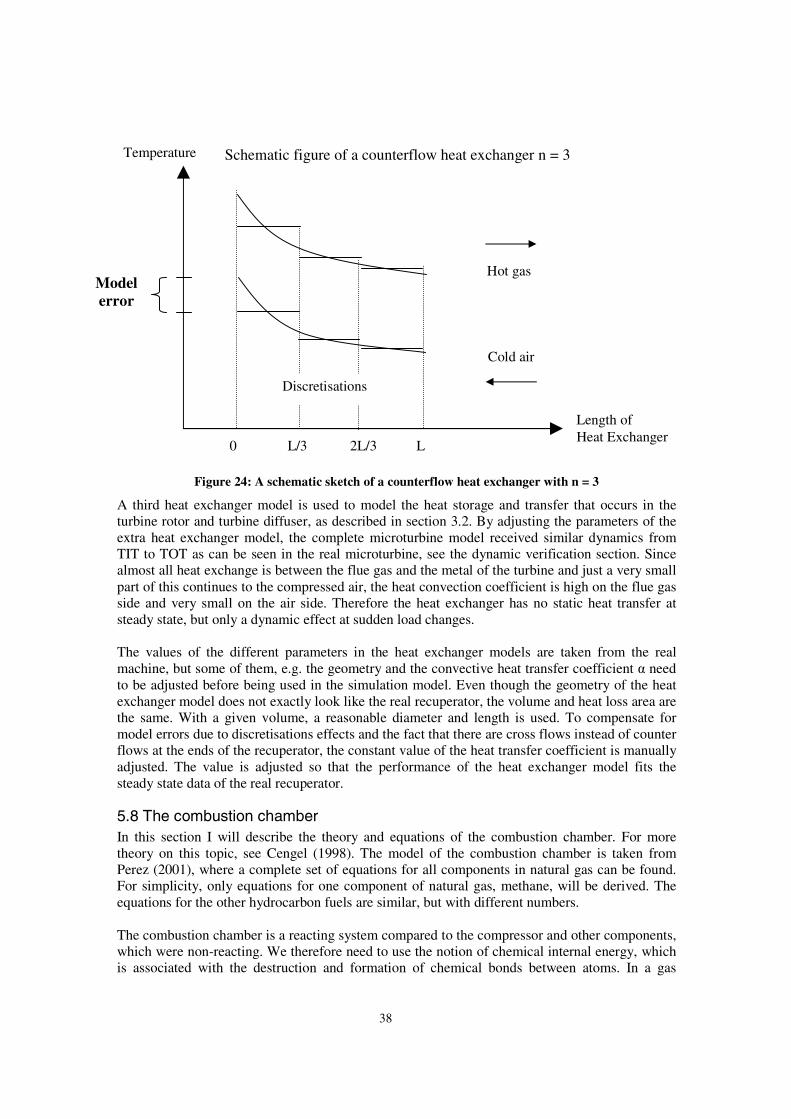
38

Figure 24: A schematic sketch of a counterflow heat exchanger with n = 3

A third heat exchanger model is used to model the heat storage and transfer that occurs in theturbine rotor and turbine diffuser, as described in section 3.2. By adjusting the parameters of theextra heat exchanger model, the complete microturbine model received similar dynamics fromTIT to TOT as can be seen in the real microturbine, see the dynamic verification section. Sincealmost all heat exchange is between the flue gas and the metal of the turbine and just a very smallpart of this continues to the compressed air, the heat convection coefficient is high on the flue gasside and very small on the air side. Therefore the heat exchanger has no static heat transfer atsteady state, but only a dynamic effect at sudden load changes.

The values of the different parameters in the heat exchanger models are taken from the realmachine, but some of them, e.g. the geometry and the convective heat transfer coefficient α needto be adjusted before being used in the simulation model. Even though the geometry of the heatexchanger model does not exactly look like the real recuperator, the volume and heat loss area arethe same. With a given volume, a reasonable diameter and length is used. To compensate formodel errors due to discretisations effects and the fact that there are cross flows instead of counterflows at the ends of the recuperator, the constant value of the heat transfer coefficient is manuallyadjusted. The value is adjusted so that the performance of the heat exchanger model fits thesteady state data of the real recuperator.

5.8 The combustion chamberIn this section I will describe the theory and equations of the combustion chamber. For moretheory on this topic, see Cengel (1998). The model of the combustion chamber is taken fromPerez (2001), where a complete set of equations for all components in natural gas can be found.For simplicity, only equations for one component of natural gas, methane, will be derived. Theequations for the other hydrocarbon fuels are similar, but with different numbers.

The combustion chamber is a reacting system compared to the compressor and other components,which were non-reacting. We therefore need to use the notion of chemical internal energy, whichis associated with the destruction and formation of chemical bonds between atoms. In a gas

Length ofHeat Exchanger

Temperature

Hot gas

Cold air

Discretisations

0 LL/3 2L/3

Schematic figure of a counterflow heat exchanger n = 3

Modelerror

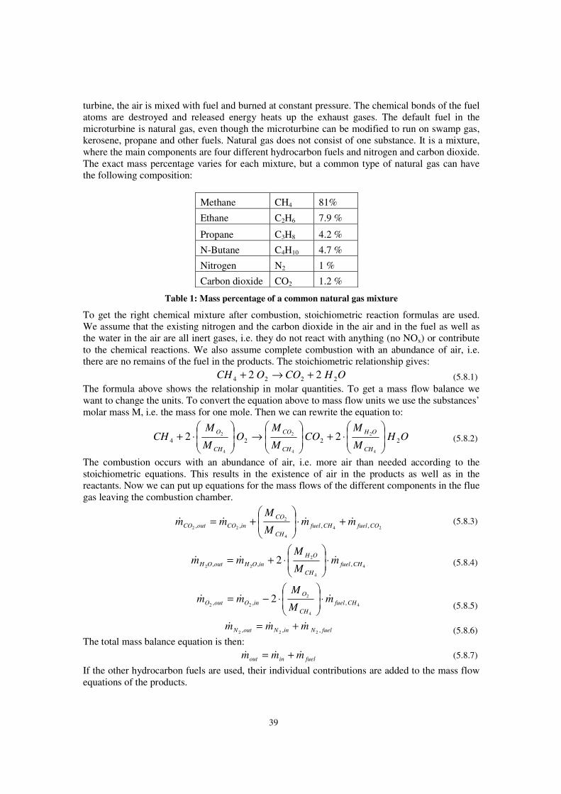
39

(5.8.1)

(5.8.2)

(5.8.7)

(5.8.3)

(5.8.4)

(5.8.5)

(5.8.6)

turbine, the air is mixed with fuel and burned at constant pressure. The chemical bonds of the fuelatoms are destroyed and released energy heats up the exhaust gases. The default fuel in themicroturbine is natural gas, even though the microturbine can be modified to run on swamp gas,kerosene, propane and other fuels. Natural gas does not consist of one substance. It is a mixture,where the main components are four different hydrocarbon fuels and nitrogen and carbon dioxide.The exact mass percentage varies for each mixture, but a common type of natural gas can havethe following composition:

Methane CH4 81%

Ethane C2H6 7.9 %

Propane C3H8 4.2 %

N-Butane C4H10 4.7 %

Nitrogen N2 1 %

Carbon dioxide CO2 1.2 %

Table 1: Mass percentage of a common natural gas mixture

To get the right chemical mixture after combustion, stoichiometric reaction formulas are used.We assume that the existing nitrogen and the carbon dioxide in the air and in the fuel as well asthe water in the air are all inert gases, i.e. they do not react with anything (no NOx) or contributeto the chemical reactions. We also assume complete combustion with an abundance of air, i.e.there are no remains of the fuel in the products. The stoichiometric relationship gives:

OHCOOCH 2224 22 +→+The formula above shows the relationship in molar quantities. To get a mass flow balance wewant to change the units. To convert the equation above to mass flow units we use the substances’molar mass M, i.e. the mass for one mole. Then we can rewrite the equation to:

OHM

MCO

M

MO

M

MCH

CH

OH

CH

CO

CH

O2224

4

2

4

2

4

2 22

⋅+

→

⋅+

The combustion occurs with an abundance of air, i.e. more air than needed according to thestoichiometric equations. This results in the existence of air in the products as well as in thereactants. Now we can put up equations for the mass flows of the different components in the fluegas leaving the combustion chamber.

24

4

2

22 ,,,, COfuelCHfuelCH

CO

inCOoutCO mmM

Mmm &&&& +⋅

+=

4

4

2

22 ,,, 2 CHfuelCH

OH

inOHoutOH mM

Mmm &&& ⋅

⋅+=

4

4

2

22 ,,, 2 CHfuelCH

O

inOoutO mM

Mmm &&& ⋅

⋅−=

fuelNinNoutN mmm ,,, 222&&& +=

The total mass balance equation is then:

fuelinout mmm &&& +=If the other hydrocarbon fuels are used, their individual contributions are added to the mass flowequations of the products.

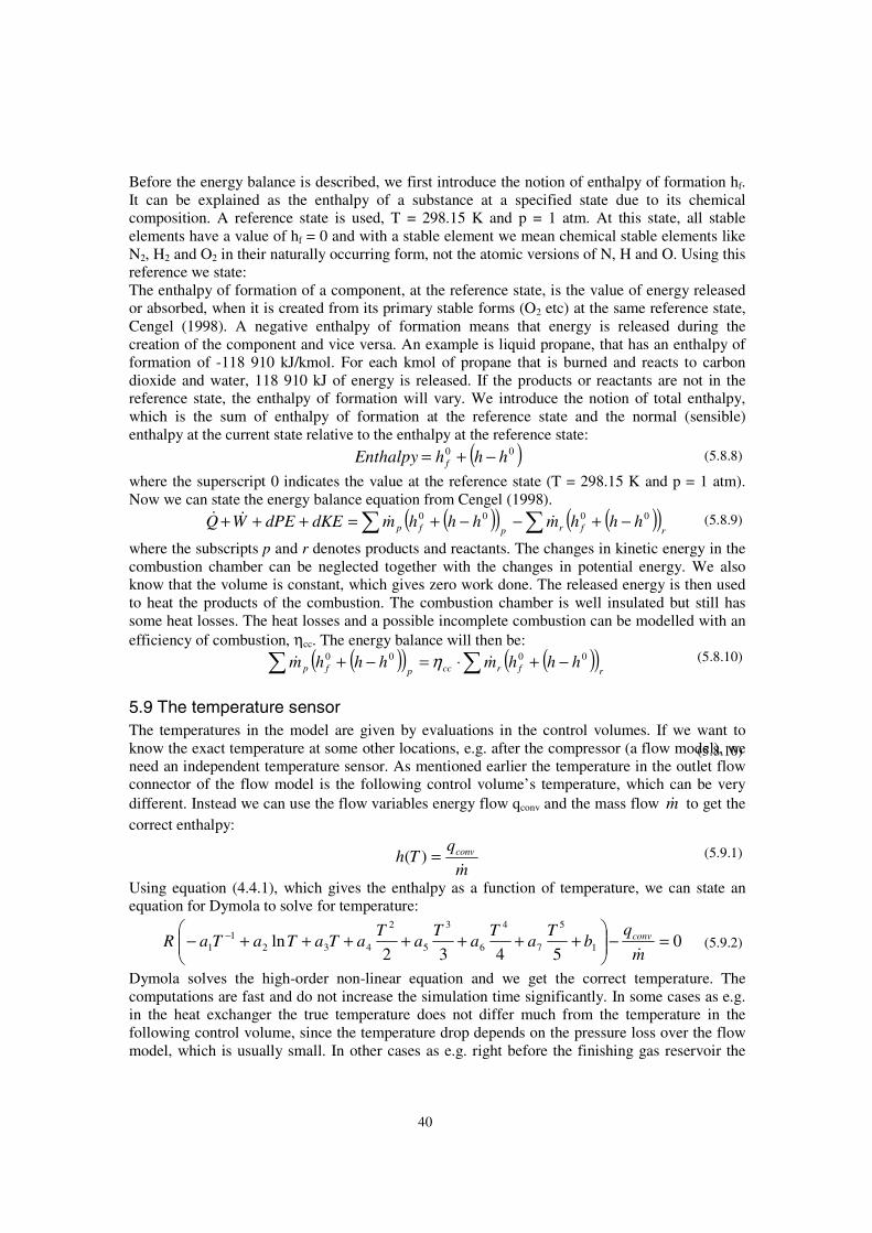
40

(5.8.8)

(5.8.9)

(5.8.10)

(5.9.1)

(5.9.2)

(5.8.10)

Before the energy balance is described, we first introduce the notion of enthalpy of formation hf.It can be explained as the enthalpy of a substance at a specified state due to its chemicalcomposition. A reference state is used, T = 298.15 K and p = 1 atm. At this state, all stableelements have a value of hf = 0 and with a stable element we mean chemical stable elements likeN2, H2 and O2 in their naturally occurring form, not the atomic versions of N, H and O. Using thisreference we state:The enthalpy of formation of a component, at the reference state, is the value of energy releasedor absorbed, when it is created from its primary stable forms (O2 etc) at the same reference state,Cengel (1998). A negative enthalpy of formation means that energy is released during thecreation of the component and vice versa. An example is liquid propane, that has an enthalpy offormation of -118 910 kJ/kmol. For each kmol of propane that is burned and reacts to carbondioxide and water, 118 910 kJ of energy is released. If the products or reactants are not in thereference state, the enthalpy of formation will vary. We introduce the notion of total enthalpy,which is the sum of enthalpy of formation at the reference state and the normal (sensible)enthalpy at the current state relative to the enthalpy at the reference state:

( )00 hhhEnthalpy f −+=where the superscript 0 indicates the value at the reference state (T = 298.15 K and p = 1 atm).Now we can state the energy balance equation from Cengel (1998).

( )( ) ( )( )∑∑ −+−−+=+++rfrpfp hhhmhhhmdKEdPEWQ 0000 &&&&

where the subscripts p and r denotes products and reactants. The changes in kinetic energy in thecombustion chamber can be neglected together with the changes in potential energy. We alsoknow that the volume is constant, which gives zero work done. The released energy is then usedto heat the products of the combustion. The combustion chamber is well insulated but still hassome heat losses. The heat losses and a possible incomplete combustion can be modelled with anefficiency of combustion, ηcc. The energy balance will then be:

( )( ) ( )( )∑∑ −+⋅=−+rfrccpfp hhhmhhhm 0000 && η

5.9 The temperature sensorThe temperatures in the model are given by evaluations in the control volumes. If we want toknow the exact temperature at some other locations, e.g. after the compressor (a flow model), weneed an independent temperature sensor. As mentioned earlier the temperature in the outlet flowconnector of the flow model is the following control volume’s temperature, which can be verydifferent. Instead we can use the flow variables energy flow qconv and the mass flow m& to get thecorrect enthalpy:

m

qTh conv

&=)(

Using equation (4.4.1), which gives the enthalpy as a function of temperature, we can state anequation for Dymola to solve for temperature:

05432

ln 1

5

7

4

6

3

5

2

4321

1 =−

+++++++− −

m

qb

Ta

Ta

Ta

TaTaTaTaR conv

&

Dymola solves the high-order non-linear equation and we get the correct temperature. Thecomputations are fast and do not increase the simulation time significantly. In some cases as e.g.in the heat exchanger the true temperature does not differ much from the temperature in thefollowing control volume, since the temperature drop depends on the pressure loss over the flowmodel, which is usually small. In other cases as e.g. right before the finishing gas reservoir the

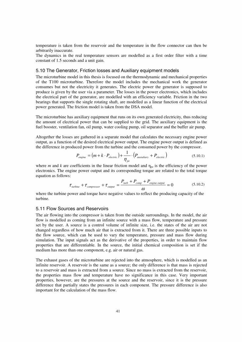
41

(5.10.1)

(5.10.2)

temperature is taken from the reservoir and the temperature in the flow connector can then bearbitrarily inaccurate.The dynamics in the real temperature sensors are modelled as a first order filter with a timeconstant of 1.5 seconds and a unit gain.

5.10 The Generator, Friction losses and Auxiliary equipment modelsThe microturbine model in this thesis is focused on the thermodynamic and mechanical propertiesof the T100 microturbine. Therefore the model includes the mechanical work the generatorconsumes but not the electricity it generates. The electric power the generator is supposed toproduce is given by the user via a parameter. The losses in the power electronics, which includesthe electrical part of the generator, are modelled with an efficiency variable. Friction in the twobearings that supports the single rotating shaft, are modelled as a linear function of the electricalpower generated. The friction model is taken from the DSA model.

The microturbine has auxiliary equipment that runs on its own generated electricity, thus reducingthe amount of electrical power that can be supplied to the grid. The auxiliary equipment is thefuel booster, ventilation fan, oil pump, water cooling pump, oil separator and the buffer air pump.

Altogether the losses are gathered in a separate model that calculates the necessary engine poweroutput, as a function of the desired electrical power output. The engine power output is defined asthe difference in produced power from the turbine and the consumed power by the compressor.

( ) ( )electricauxialiarype

electricengine PPPkmP +⋅+⋅+=η

1

where m and k are coefficients in the linear friction model and ηpe is the efficiency of the powerelectronics. The engine power output and its corresponding torque are related to the total torqueequation as follows:

0=++

=++ω

τττ outputenginecompturboutputcompressorturbine

PPP

where the turbine power and torque have negative values to reflect the producing capacity of theturbine.

5.11 Flow Sources and ReservoirsThe air flowing into the compressor is taken from the outside surroundings. In the model, the airflow is modelled as coming from an infinite source with a mass flow, temperature and pressureset by the user. A source is a control volume of infinite size, i.e. the states of the air are notchanged regardless of how much air that is extracted from it. There are three possible inputs tothe flow source, which can be used to vary the temperature, pressure and mass flow duringsimulation. The input signals act as the derivative of the properties, in order to maintain flowproperties that are differentiable. In the source, the initial chemical composition is set if themedium has more than one component, e.g. air or natural gas.

The exhaust gases of the microturbine are rejected into the atmosphere, which is modelled as aninfinite reservoir. A reservoir is the same as a source; the only difference is that mass is rejectedto a reservoir and mass is extracted from a source. Since no mass is extracted from the reservoir,the properties mass flow and temperature have no significance in this case. Very importantproperties, however, are the pressures at the source and the reservoir, since it is the pressuredifference that partially states the pressures in each component. The pressure difference is alsoimportant for the calculation of the mass flow.

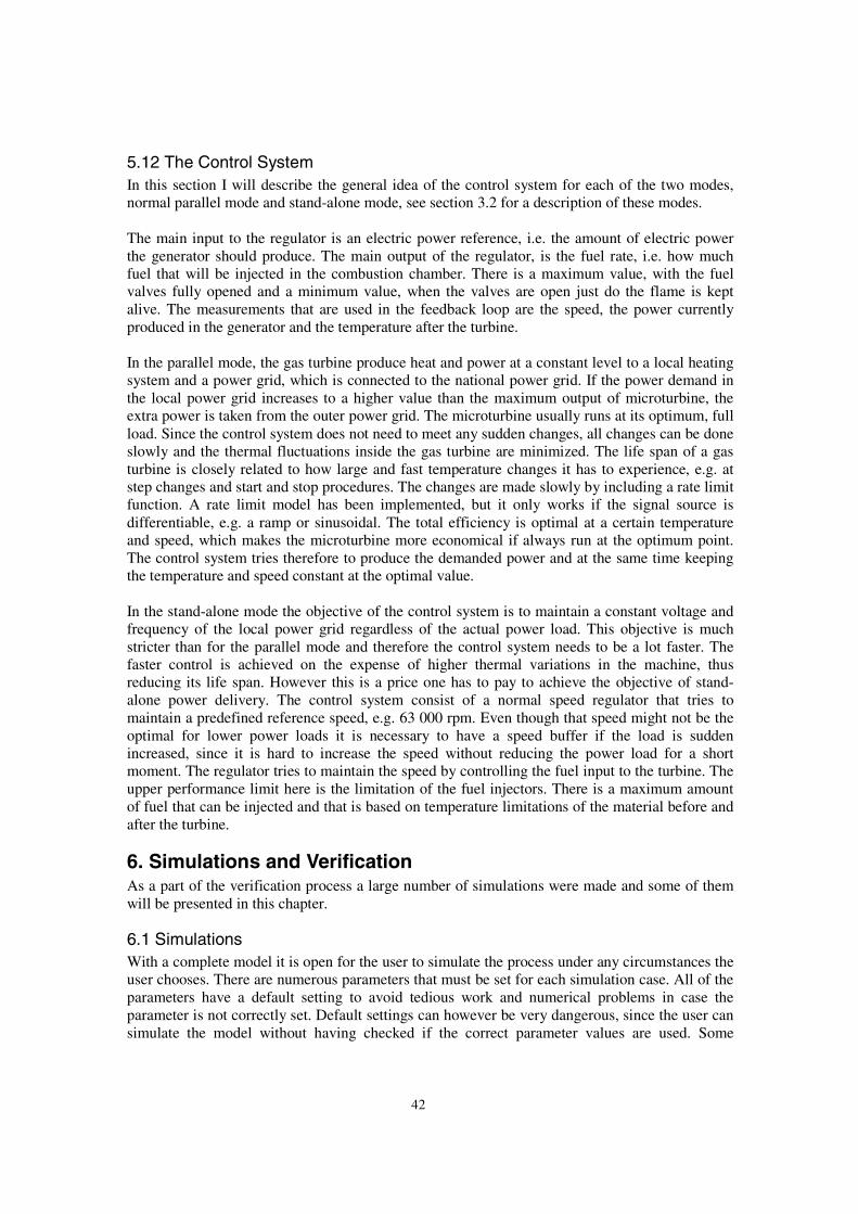
42

5.12 The Control SystemIn this section I will describe the general idea of the control system for each of the two modes,normal parallel mode and stand-alone mode, see section 3.2 for a description of these modes.

The main input to the regulator is an electric power reference, i.e. the amount of electric powerthe generator should produce. The main output of the regulator, is the fuel rate, i.e. how muchfuel that will be injected in the combustion chamber. There is a maximum value, with the fuelvalves fully opened and a minimum value, when the valves are open just do the flame is keptalive. The measurements that are used in the feedback loop are the speed, the power currentlyproduced in the generator and the temperature after the turbine.

In the parallel mode, the gas turbine produce heat and power at a constant level to a local heatingsystem and a power grid, which is connected to the national power grid. If the power demand inthe local power grid increases to a higher value than the maximum output of microturbine, theextra power is taken from the outer power grid. The microturbine usually runs at its optimum, fullload. Since the control system does not need to meet any sudden changes, all changes can be doneslowly and the thermal fluctuations inside the gas turbine are minimized. The life span of a gasturbine is closely related to how large and fast temperature changes it has to experience, e.g. atstep changes and start and stop procedures. The changes are made slowly by including a rate limitfunction. A rate limit model has been implemented, but it only works if the signal source isdifferentiable, e.g. a ramp or sinusoidal. The total efficiency is optimal at a certain temperatureand speed, which makes the microturbine more economical if always run at the optimum point.The control system tries therefore to produce the demanded power and at the same time keepingthe temperature and speed constant at the optimal value.

In the stand-alone mode the objective of the control system is to maintain a constant voltage andfrequency of the local power grid regardless of the actual power load. This objective is muchstricter than for the parallel mode and therefore the control system needs to be a lot faster. Thefaster control is achieved on the expense of higher thermal variations in the machine, thusreducing its life span. However this is a price one has to pay to achieve the objective of stand-alone power delivery. The control system consist of a normal speed regulator that tries tomaintain a predefined reference speed, e.g. 63 000 rpm. Even though that speed might not be theoptimal for lower power loads it is necessary to have a speed buffer if the load is suddenincreased, since it is hard to increase the speed without reducing the power load for a shortmoment. The regulator tries to maintain the speed by controlling the fuel input to the turbine. Theupper performance limit here is the limitation of the fuel injectors. There is a maximum amountof fuel that can be injected and that is based on temperature limitations of the material before andafter the turbine.

6. Simulations and VerificationAs a part of the verification process a large number of simulations were made and some of themwill be presented in this chapter.

6.1 SimulationsWith a complete model it is open for the user to simulate the process under any circumstances theuser chooses. There are numerous parameters that must be set for each simulation case. All of theparameters have a default setting to avoid tedious work and numerical problems in case theparameter is not correctly set. Default settings can however be very dangerous, since the user cansimulate the model without having checked if the correct parameter values are used. Some

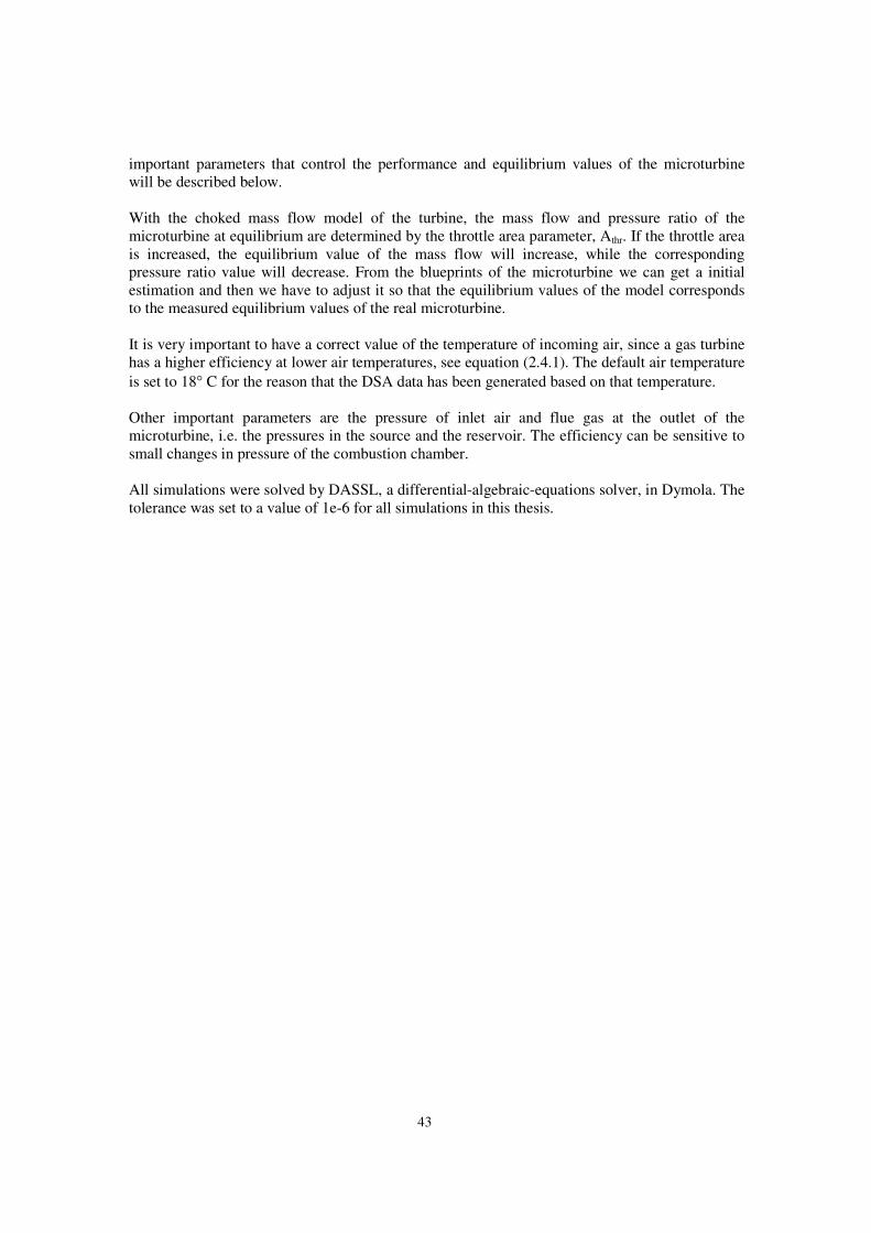
43

important parameters that control the performance and equilibrium values of the microturbinewill be described below.

With the choked mass flow model of the turbine, the mass flow and pressure ratio of themicroturbine at equilibrium are determined by the throttle area parameter, Athr. If the throttle areais increased, the equilibrium value of the mass flow will increase, while the correspondingpressure ratio value will decrease. From the blueprints of the microturbine we can get a initialestimation and then we have to adjust it so that the equilibrium values of the model correspondsto the measured equilibrium values of the real microturbine.

It is very important to have a correct value of the temperature of incoming air, since a gas turbinehas a higher efficiency at lower air temperatures, see equation (2.4.1). The default air temperatureis set to 18° C for the reason that the DSA data has been generated based on that temperature.

Other important parameters are the pressure of inlet air and flue gas at the outlet of themicroturbine, i.e. the pressures in the source and the reservoir. The efficiency can be sensitive tosmall changes in pressure of the combustion chamber.

All simulations were solved by DASSL, a differential-algebraic-equations solver, in Dymola. Thetolerance was set to a value of 1e-6 for all simulations in this thesis.

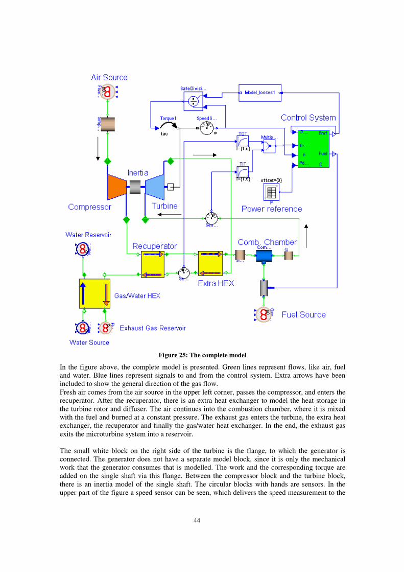
44

Figure 25: The complete model

In the figure above, the complete model is presented. Green lines represent flows, like air, fueland water. Blue lines represent signals to and from the control system. Extra arrows have beenincluded to show the general direction of the gas flow.Fresh air comes from the air source in the upper left corner, passes the compressor, and enters therecuperator. After the recuperator, there is an extra heat exchanger to model the heat storage inthe turbine rotor and diffuser. The air continues into the combustion chamber, where it is mixedwith the fuel and burned at a constant pressure. The exhaust gas enters the turbine, the extra heatexchanger, the recuperator and finally the gas/water heat exchanger. In the end, the exhaust gasexits the microturbine system into a reservoir.

The small white block on the right side of the turbine is the flange, to which the generator isconnected. The generator does not have a separate model block, since it is only the mechanicalwork that the generator consumes that is modelled. The work and the corresponding torque areadded on the single shaft via this flange. Between the compressor block and the turbine block,there is an inertia model of the single shaft. The circular blocks with hands are sensors. In theupper part of the figure a speed sensor can be seen, which delivers the speed measurement to the

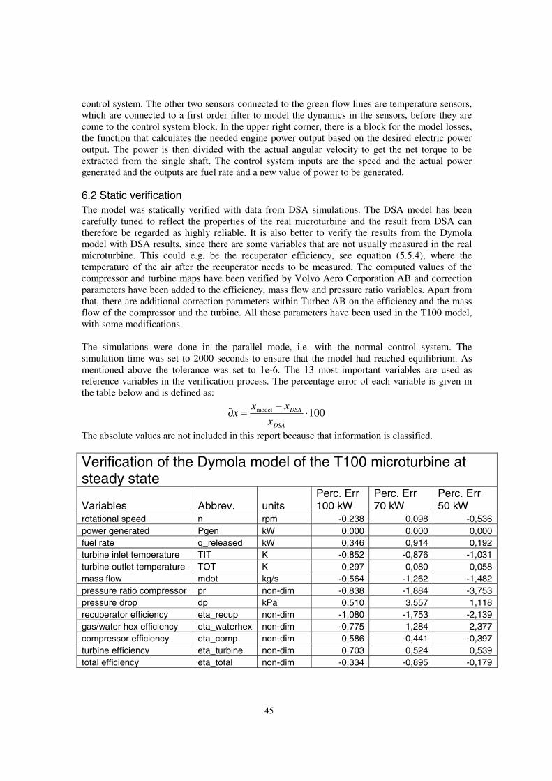
45

control system. The other two sensors connected to the green flow lines are temperature sensors,which are connected to a first order filter to model the dynamics in the sensors, before they arecome to the control system block. In the upper right corner, there is a block for the model losses,the function that calculates the needed engine power output based on the desired electric poweroutput. The power is then divided with the actual angular velocity to get the net torque to beextracted from the single shaft. The control system inputs are the speed and the actual powergenerated and the outputs are fuel rate and a new value of power to be generated.

6.2 Static verificationThe model was statically verified with data from DSA simulations. The DSA model has beencarefully tuned to reflect the properties of the real microturbine and the result from DSA cantherefore be regarded as highly reliable. It is also better to verify the results from the Dymolamodel with DSA results, since there are some variables that are not usually measured in the realmicroturbine. This could e.g. be the recuperator efficiency, see equation (5.5.4), where thetemperature of the air after the recuperator needs to be measured. The computed values of thecompressor and turbine maps have been verified by Volvo Aero Corporation AB and correctionparameters have been added to the efficiency, mass flow and pressure ratio variables. Apart fromthat, there are additional correction parameters within Turbec AB on the efficiency and the massflow of the compressor and the turbine. All these parameters have been used in the T100 model,with some modifications.

The simulations were done in the parallel mode, i.e. with the normal control system. Thesimulation time was set to 2000 seconds to ensure that the model had reached equilibrium. Asmentioned above the tolerance was set to 1e-6. The 13 most important variables are used asreference variables in the verification process. The percentage error of each variable is given inthe table below and is defined as:

100model ⋅−

=∂DSA

DSA

x

xxx

The absolute values are not included in this report because that information is classified.

Verification of the Dymola model of the T100 microturbine atsteady state

Variables Abbrev. unitsPerc. Err100 kW

Perc. Err70 kW

Perc. Err50 kW

rotational speed n rpm -0,238 0,098 -0,536power generated Pgen kW 0,000 0,000 0,000fuel rate q_released kW 0,346 0,914 0,192turbine inlet temperature TIT K -0,852 -0,876 -1,031turbine outlet temperature TOT K 0,297 0,080 0,058mass flow mdot kg/s -0,564 -1,262 -1,482pressure ratio compressor pr non-dim -0,838 -1,884 -3,753pressure drop dp kPa 0,510 3,557 1,118recuperator efficiency eta_recup non-dim -1,080 -1,753 -2,139gas/water hex efficiency eta_waterhex non-dim -0,775 1,284 2,377compressor efficiency eta_comp non-dim 0,586 -0,441 -0,397turbine efficiency eta_turbine non-dim 0,703 0,524 0,539total efficiency eta_total non-dim -0,334 -0,895 -0,179

46

Table 2: Results from static verification with data from DSA simulations

The average error is 0.61%, 1.2% and 1.1% for the 100 kW, 70 kW and 50 kW case. A few largererrors such as the pressure drop and the pressure ratio increase the average error significantly forthe part load cases.

Power generated: This is the most important output and should therefore be exactly the same asthe reference power. This is accomplished by the control system and is not really a verification ofthe thermodynamic model, but rather a verification of the control system.Speed: The speed variable shows indirect efficiency of the model. If the speed of the model islower than the speed data from DSA, the efficiency of the model is too high, because the modelcan have a lower speed and still produce the same electric power output.TIT (temperature at the inlet of the turbine): This variable is used in the control system and islimiting the efficiency, since the turbine blades have a maximum temperature they are designed tosustain.TOT (temperature at the outlet of the turbine): This variable is also used in the control systemand limits the efficiency, but in this case it is the recuperator that cannot sustain too hightemperatures without breaking.Pressure ratio over the compressor: In the verification process, there has to be at least onepressure measurement. The value of the pressure ratio is better than an absolute pressure valuesince the pressure ratio is dimensionless and therefore not influenced by the pressure of theambient air at the inlet. The pressure ratio over the turbine could have been used without anydifferences.Added fuel power: This variable shows how much fuel has been used in the unit kW. The fuelpower is preferred over the variable fuel mass flow since different fuels have different energy ofcombustion.The mass flow through the compressor: This is one of the most important variables. The massflow through the turbine could also been used without any difference.Pressure drop from the compressor to the turbine: This variable gives information about howaccurate the pressure drop models used in the heat exchangers and the combustion chamber.Efficiency of the recuperator: This variable shows how well the recuperator works. Anothervariable that could have been used was total heat transferred in the recuperator, but as for asimilar reason as above a dimensionless variable is preferable.Efficiency of the gas/water heat exchanger: Same as above but for the gas/water heatexchanger instead.Efficiency of the compressor: Since this is a variable that is difficult to model, it is important toverify the results of the model.Efficiency of the turbine: Same as above.Total efficiency: This important variable tells us if the complete model has the same performanceas the real microturbine.

From the results of the static verification above, we see that the largest error is in the compressormass flow and pressure ratio. In a model, where the complete microturbine system is emphasized,the errors of 2-4% can be acceptable. The errors are probably caused by errors in the ellipsoidcurves that model the compressor mass flow. The pressure ratio and the mass flow for a certainspeed are uniquely determined by the ellipsoid curve for that particular speed, see figure 16. Withcorrection parameters, the equilibrium point can be adjusted and moved along the curve. In thismodel, both mass flow and pressure ratio are too low, which means that the true equilibrium pointlies above the model curve. Therefore the errors of the mass flow and pressure ratio have a closerelation. The error of the turbine mass flow model at lower part load might also increase the errorof the compressor mass flow. In Gustafsson (1998), it was also the compressor mass flow model

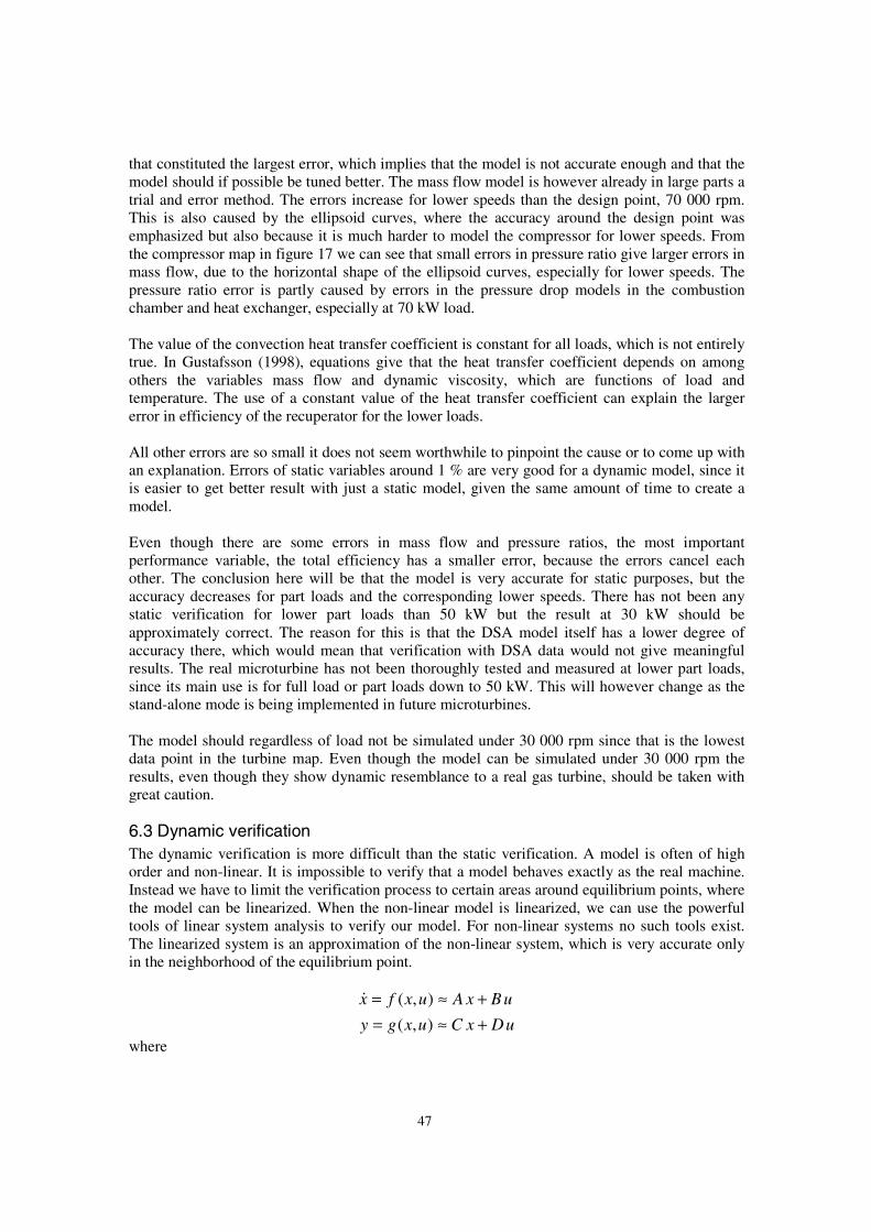
47

that constituted the largest error, which implies that the model is not accurate enough and that themodel should if possible be tuned better. The mass flow model is however already in large parts atrial and error method. The errors increase for lower speeds than the design point, 70 000 rpm.This is also caused by the ellipsoid curves, where the accuracy around the design point wasemphasized but also because it is much harder to model the compressor for lower speeds. Fromthe compressor map in figure 17 we can see that small errors in pressure ratio give larger errors inmass flow, due to the horizontal shape of the ellipsoid curves, especially for lower speeds. Thepressure ratio error is partly caused by errors in the pressure drop models in the combustionchamber and heat exchanger, especially at 70 kW load.

The value of the convection heat transfer coefficient is constant for all loads, which is not entirelytrue. In Gustafsson (1998), equations give that the heat transfer coefficient depends on amongothers the variables mass flow and dynamic viscosity, which are functions of load andtemperature. The use of a constant value of the heat transfer coefficient can explain the largererror in efficiency of the recuperator for the lower loads.

All other errors are so small it does not seem worthwhile to pinpoint the cause or to come up withan explanation. Errors of static variables around 1 % are very good for a dynamic model, since itis easier to get better result with just a static model, given the same amount of time to create amodel.

Even though there are some errors in mass flow and pressure ratios, the most importantperformance variable, the total efficiency has a smaller error, because the errors cancel eachother. The conclusion here will be that the model is very accurate for static purposes, but theaccuracy decreases for part loads and the corresponding lower speeds. There has not been anystatic verification for lower part loads than 50 kW but the result at 30 kW should beapproximately correct. The reason for this is that the DSA model itself has a lower degree ofaccuracy there, which would mean that verification with DSA data would not give meaningfulresults. The real microturbine has not been thoroughly tested and measured at lower part loads,since its main use is for full load or part loads down to 50 kW. This will however change as thestand-alone mode is being implemented in future microturbines.

The model should regardless of load not be simulated under 30 000 rpm since that is the lowestdata point in the turbine map. Even though the model can be simulated under 30 000 rpm theresults, even though they show dynamic resemblance to a real gas turbine, should be taken withgreat caution.

6.3 Dynamic verificationThe dynamic verification is more difficult than the static verification. A model is often of highorder and non-linear. It is impossible to verify that a model behaves exactly as the real machine.Instead we have to limit the verification process to certain areas around equilibrium points, wherethe model can be linearized. When the non-linear model is linearized, we can use the powerfultools of linear system analysis to verify our model. For non-linear systems no such tools exist.The linearized system is an approximation of the non-linear system, which is very accurate onlyin the neighborhood of the equilibrium point.

uDxCuxgy

uBxAuxfx

+≈=+≈=

),(

),(&

where

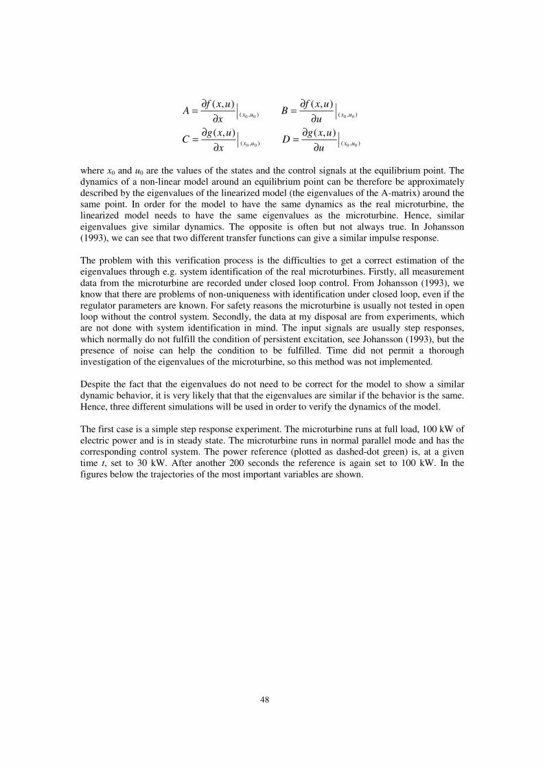
48

),(),(

),(),(

0000

0000

),(),(

),(),(

uxux

uxux

u

uxgD

x

uxgC

u

uxfB

x

uxfA

∂∂=

∂∂=

∂∂=

∂∂=

where x0 and u0 are the values of the states and the control signals at the equilibrium point. Thedynamics of a non-linear model around an equilibrium point can be therefore be approximatelydescribed by the eigenvalues of the linearized model (the eigenvalues of the A-matrix) around thesame point. In order for the model to have the same dynamics as the real microturbine, thelinearized model needs to have the same eigenvalues as the microturbine. Hence, similareigenvalues give similar dynamics. The opposite is often but not always true. In Johansson(1993), we can see that two different transfer functions can give a similar impulse response.

The problem with this verification process is the difficulties to get a correct estimation of theeigenvalues through e.g. system identification of the real microturbines. Firstly, all measurementdata from the microturbine are recorded under closed loop control. From Johansson (1993), weknow that there are problems of non-uniqueness with identification under closed loop, even if theregulator parameters are known. For safety reasons the microturbine is usually not tested in openloop without the control system. Secondly, the data at my disposal are from experiments, whichare not done with system identification in mind. The input signals are usually step responses,which normally do not fulfill the condition of persistent excitation, see Johansson (1993), but thepresence of noise can help the condition to be fulfilled. Time did not permit a thoroughinvestigation of the eigenvalues of the microturbine, so this method was not implemented.

Despite the fact that the eigenvalues do not need to be correct for the model to show a similardynamic behavior, it is very likely that that the eigenvalues are similar if the behavior is the same.Hence, three different simulations will be used in order to verify the dynamics of the model.

The first case is a simple step response experiment. The microturbine runs at full load, 100 kW ofelectric power and is in steady state. The microturbine runs in normal parallel mode and has thecorresponding control system. The power reference (plotted as dashed-dot green) is, at a giventime t, set to 30 kW. After another 200 seconds the reference is again set to 100 kW. In thefigures below the trajectories of the most important variables are shown.

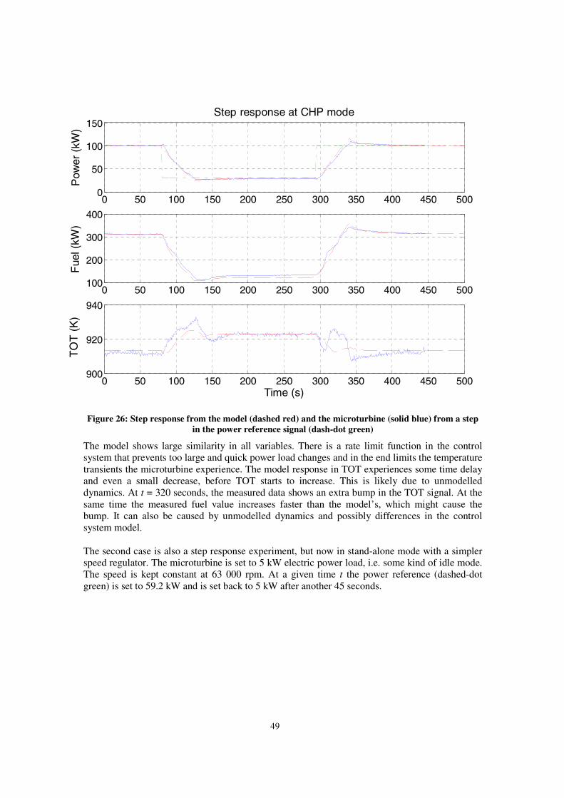
49

0 50 100 150 200 250 300 350 400 450 5000

50

100

150

Pow

er (

kW)

Step response at CHP mode

0 50 100 150 200 250 300 350 400 450 500100

200

300

400

Fue

l (kW

)

0 50 100 150 200 250 300 350 400 450 500900

920

940

Time (s)

TO

T (

K)

Figure 26: Step response from the model (dashed red) and the microturbine (solid blue) from a stepin the power reference signal (dash-dot green)

The model shows large similarity in all variables. There is a rate limit function in the controlsystem that prevents too large and quick power load changes and in the end limits the temperaturetransients the microturbine experience. The model response in TOT experiences some time delayand even a small decrease, before TOT starts to increase. This is likely due to unmodelleddynamics. At t = 320 seconds, the measured data shows an extra bump in the TOT signal. At thesame time the measured fuel value increases faster than the model’s, which might cause thebump. It can also be caused by unmodelled dynamics and possibly differences in the controlsystem model.

The second case is also a step response experiment, but now in stand-alone mode with a simplerspeed regulator. The microturbine is set to 5 kW electric power load, i.e. some kind of idle mode.The speed is kept constant at 63 000 rpm. At a given time t the power reference (dashed-dotgreen) is set to 59.2 kW and is set back to 5 kW after another 45 seconds.

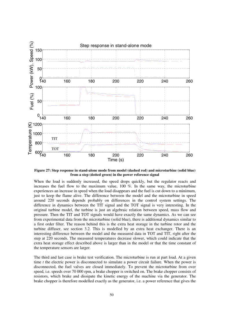
50

140 160 180 200 220 240 2600

50

100

150

Pow

er (

kW),

Spe

ed (

%)

Step response in stand-alone mode

140 160 180 200 220 240 2600

50

100

Fue

l (%

)

140 160 180 200 220 240 260600

800

1000

1200

Time (s)

Tem

pera

ture

(K

)

Figure 27: Step response in stand-alone mode from model (dashed red) and microturbine (solid blue)from a step (dotted green) in the power reference signal

When the load is suddenly increased, the speed drops quickly, but the regulator reacts andincreases the fuel flow to the maximum value, 100 %. In the same way, the microturbineexperiences an increase in speed when the load disappears and the fuel is cut down to a minimum,just to keep the flame alive. The difference between the model and the microturbine in speedaround 220 seconds depends probably on differences in the control system settings. Thedifference in dynamics between the TIT signal and the TOT signal is very interesting. In theoriginal turbine model, the turbine is just an algebraic relation between speed, mass flow andpressure. Then the TIT and TOT signals would have exactly the same dynamics. As we can seefrom experimental data from the microturbine (solid blue), there is additional dynamics similar toa first order filter. The reason behind this is the extra heat storage in the turbine rotor and theturbine diffuser, see section 3.2. This is modelled by an extra heat exchanger. There is aninteresting difference between the model and the measured data in TOT and TIT, right after thestep at 220 seconds. The measured temperatures decrease slower, which could indicate that theextra heat storage effect described above is larger than in the model or that the time constant ofthe temperature sensors are larger.

The third and last case is brake test verification. The microturbine is run at part load. At a giventime t the electric power is disconnected to simulate a power circuit failure. When the power isdisconnected, the fuel valves are closed immediately. To prevent the microturbine from overspeed, i.e. speeds over 70 000 rpm, a brake chopper is switched on. The brake chopper consists ofresistors, which brake and dissipate the kinetic energy of the machine via the generator. Thebrake chopper is therefore modelled exactly as the generator, i.e. a power reference that gives the

TIT

TOT

51

engine power output. With this simulation, the most important dynamic is the speed at which themicroturbine decelerates. The axes of the figure below are removed for confidentiality.

Spe

ed (

rpm

)

Brake chopper test

Time (s)

Figure 28: Brake chopper test with data from the model (dashed red) and the microturbine (solidblue) when the power grid is disconnected at time t = 600 seconds.

The model value of the speed shows great similarity with the measured values down to 35 000rpm, which is the within the valid range of the model. The difference can be explained by twoseparate causes. Firstly, there are larger model errors at lower speeds, especially since data in thecompressor and turbine map are given down to 21 000 and 30 000 rpm respectively. Secondlyand possibly the largest error is a difference in the simple brake chopper model (the power itdissipates) and the control system model. As described in section 5.10 and figure 25 the desiredengine power output is divided with the angular velocity to get the brake chopper torque. Whenthe speed is decreasing faster than the desired power output, the torque is increased even more.As the speed goes to zero, the torque goes in theory to infinity. This effect can be seen in figure28, where the speed drops very quickly in the end.

7. Conclusions and SummaryIn this chapter I will discuss the results given in the previous chapter and give a summary of themodels used in this thesis.

The mass flow of the compressor is modelled with fitted curves, which parameters can beevaluated by polynomial functions, see figure 17. The efficiency of the compressor is modelled asparabolic degradation curves, which can be seen in figure 18. The mass flow through the turbineis modelled as choked (at a maximum) through the entire working range, see equation (5.4.1) andfigure 20. The efficiency of the turbine is computed through interpolation, see equation (5.4.4).The heat exchangers in the microturbine are modelled as pipes with heat convection andconduction in one dimension, see figure 22. The increase in enthalpy of the fluid in thecombustion chamber is based on reaction formulas and the corresponding energy released during

52

combustion, see equation (5.8.10). The generator is modelled through a torque that is put on theshaft of the compressor and the turbine, see equation (5.10.2).

7.1 Static verificationThe values of the model are very close to the data from DSA. The average errors of the variablesat the different loads are 0.6%, 1.2% and 1.1% for the 100 kW, 70 kW and 50 kW caserespectively. The emphasis in this thesis has been on the complete model of the microturbine overaccurate submodels of individual components, in order to get a complete model running early inthe project.

7.2 Dynamic verificationThe model shows a great similarity with the measured values from the real microturbine. The taskof tuning a dynamic model is an incredible difficult task, since there are a vast number ofparameters with strong coupling effects to each other. As discussed earlier, the verification shouldbe done in open loop simulations, so that differences in the control system models would notaffect the results. I have chosen the verification simulations, so that as much as possible of thedynamics of the model should be verified. Still there are more verification simulations to be doneif one wants to cover all possible operations and if the dynamics should be verified beyondreasonable doubt, then system identification must be made on the microturbine.

7.3 Valid operating ranges for the modelOne of the most important things to know about a model is not exactly how accurate it is, but inwhich areas it is verified and validated. All the components have a range of operation and thelimiting components are listed below.

The medium used is a mixture of carbon dioxide, water vapor, oxygen and nitrogen. The data thatgives the thermodynamic property of a substance is valid at temperatures from 200 K up to 6000K. The water vapor model does not handle the condensation of water in the fog region fortemperatures below the dew point temperature, but the compressor quickly heats the gas so thepossible effect can be neglected.

The compressor and turbine data implemented in the model cover speeds from 74 000 rpm downto 21 000 rpm and 30 000 rpm respectively. The model should therefore not be used under 30 000rpm, even though it is numerically possible to simulate the microturbine down to 15 000 rpm.Between 30 000 rpm and 15 000 rpm the model have a behavior that resembles a gas turbine, butthe results should used with great caution.

The model is statically verified down to 50 kW part load with high accuracy. It is very likely thatthe model has an acceptable accuracy even down to 30 kW part load.

8. Possible Applications and Future WorkA model is never perfect. There are always things to be improved, but there is also a trade-offbetween time spent on a component and the component’s functionality and value in the model.The same reason goes for more detailed modelling. A functional model as been developed and themodel can surely be made more detailed, but the question is, is it worth the extra time spent? If itis, then one might do it later when the need arises. But the most important thing is to get acomplete model running and then choose what part we want to study further.

53

As described earlier in the thesis, there are many possibilities for this model. After verificationand testing of the model, there are a lot of possible applications:

• The model can be used in What-if studies at internal and external dynamic changes, i.e.what happens e.g. with the temperature after the turbine if the load changes or if thetemperature of the ambient air is suddenly changed

• The model can be used to design control strategies, e.g. when using a brake chopper.• The model can be used to evaluate new developments in the control system for the stand-

alone mode, before tried on a real microturbine.

Suggestions for future work:• The existing rate limit model does work for discrete time, but in continuous time it can

only be used if the source is analytically differentiable, e.g. a sinusoidal or ramp signal.The model should be able to deal with signals that are not directly differentiable, i.e.signals from time tables or if the rate limit model is placed far away from the source.

• Developing an operator interface with the LabVIEW program in real time for operatortraining.

• With the LabVIEW application, it can be possible to initiate hardware/software failures,so that service technicians/engineers can learn how the gas turbine behaves with a similarfailure.

• The bypass function was never fully modelled and should be completed if such interestarises.

• The medium models can be changed into models that uses fewer individual substancesand instead a constant composition, thus reducing the number of states in the model. Withfewer states the simulation time will decrease and the model will be easier to linearizeand to use in state-space equations in control design.

• The heat exchanger might be modelled with the log-mean temperature method. It mightthen be possible to reduce the number of discretisations used in the heat exchanger andtherefore the number of states in the model. It is however not obvious that the dynamicbehavior will not be changed.

• Development of a model of the power electronics so that the complete machine can besimulated against a power grid.

• With a power electronics model, the complete power plant can be used to design andverify control strategies for power production with several machines connected inparallel.

• The model can be linearized and then used in a TOT estimator in the flame-out detectionsystem.

• The model can be linearized and put in a state-space form and then used in theoreticalcontrol design

References1. Cohen H, Rogers GFC and Saravanamuttoo HIH: “Gas Turbine Theory”. Longman Group

Ltd. 4th ed. London, 19962. Cengel Y.A and Boles M.A: “Thermodynamics, An Engineering Approach”. WCB/McGraw-

Hill 3rd ed. New York, 19983. DeWitt D.P and Incropera F.P: “Fundamentals of Heat and Mass Transfer”. Wiley 4th ed.

New York, 19964. Dynasim AB: “Dymola, Dynamic Modeling Laboratory – User’s Manual”. Dynasim AB

Lund, 2001

54

5. Eborn J: “On Model Libraries for Thermo-hydraulic Applications”. Doctoral Thesis, LundUniversity ISRN LUTFD2 / TFRT–1061–SE Lund, 2001

6. Eborn J, Tummescheit H and Åström K.J: “Physical System Modeling with Modelica™”,Lund, http://www.control.lth.se/~hubertus/ThermoFluid, 1999

7. Eborn J, Tummescheit H and Wagner F: “ThermoFlow, A Thermo-Hydraulic Library inModelica, Documentation” http://www.control.lth.se/~hubertus/ThermoFluid, 2000

8. Fox R.W and McDonald A.T: “Introduction to Fluid Mechanics”. Wiley 5th ed. New York,1998

9. Gordon S, and McBride B.J: “Computer program for calculation of complex chemicalequilibrium compositions and applications”, NASA Technical Reports Report Number:NASA-RP-1311 E-8017 NAS 1.61:1311, NASA Lewis Research Center, 1994

10. Gustafsson J.O: “Static and Dynamic Modelling of Gas Turbine in Advanced Cycles”.Licentiate Thesis, Lund University ISRN LUTMDN/TMVK 98/7030-SE Lund, 1998

11. Johansson R: “System Modelling & Identification”. Prentice Hall 1st ed. New Jersey, 199312. Malmquist A: “Analysis of a Gas Turbine Driven Hybrid Drive System for Heavy Vehicles”.

Doctoral thesis, The Royal Institute of Technology ISSN-1102-0172, Stockholm, 199913. Modelica Association: “Modelica ™ - A Unified Object-Oriented Language for Physical

Systems Modeling, Language Specification and Tutorial” www.modelica.org, 200014. Pérez Gómez A.A: “Modelling of a Gas Turbine with Modelica™”. Master Thesis, Lund

University ISRN LUTFD2/TFRT—5668—SE, Lund, 200115. Thomas P: “Simulation of Industrial Processes for Control Engineers”. Butterworth-

Heinemann 1st ed. Oxford, 199916. Tummescheit H: “Object Oriented Modeling – Design and Implementation of Libraries using

Modelica”. Doctoral thesis, to be published, Lund University, 200217. Wagner F: “The Free Modelica Editor”. http://www.et.dtu.dk/fme, 200018. Wagner W and Kruse A: “Properties of Water and Steam”, IAPWS-IF97. Springer-Verlag,

Berlin, 1998