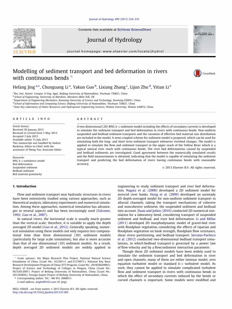
Journal of Hydrology 499 (2013) 224–235

Contents lists available at SciVerse ScienceDirect

Journal of Hydrology

journal homepage: www.elsevier .com/locate / jhydrol

Modelling of sediment transport and bed deformation in riverswith continuous bends q

0022-1694/$ - see front matter � 2013 Elsevier B.V. All rights reserved.http://dx.doi.org/10.1016/j.jhydrol.2013.07.005

q Grant sponsor: the Major Research Plan Project, National Natural ScienceFoundation of China (Grant No.: 91230111 and 51279071); National Key BasicResearch Development Program of China (973 Program, Grant No.: 2010CB429002);Project of Science and Technology of Colleges in Ningxia, China (Grant No.:NGY2012097); Project of Beifang University of Nationalities, China (Grant No.:2012XZK05); Foreign Expert Project of Beifang University of Nationalites, China.⇑ Corresponding author. Tel.: +86 951 2068011.

E-mail address: jinghef@163.com (H. Jing).

Hefang Jing a,⇑, Chunguang Li a, Yakun Guo b, Lixiang Zhang c, Lijun Zhu d, Yitian Li e

a Res. Inst. Numer. Comput. & Eng. Appl., Beifang University of Nationalities, Yinchuan 750021, Chinab School of Engineering, University of Aberdeen, Aberdeen AB24 3UE, UKc Department of Engineering Mechanics, Kunming University of Science and Technology, Kunming 650051, Chinad School of Information and Computing Science, Beifang University of Nationalities, Yinchuan 750021, Chinae State Key Laboratory of Water Resources and Hydropower Engineering Sciences, Wuhan University, Wuhan 430072, China

a r t i c l e i n f o

Article history:Received 30 January 2013Received in revised form 5 May 2013Accepted 3 July 2013Available online 15 July 2013This manuscript was handled by AndrasBardossy, Editor-in-Chief, with theassistance of Sheng Yue, Associate Editor

Keywords:RNG k–e turbulence modelBed deformationSuspended sedimentBedload sedimentBed material granularity

a b s t r a c t

A two dimensional (2D) RNG k–e sediment model including the effects of secondary currents is developedto simulate the sediment transport and bed deformation in rivers with continuous bends. Non-uniformsuspended and bedload sediment transports and the variation of effective bed material size distributionare included in the model. A semi-coupled scheme for sediment model is proposed, which can be used forsimulating both the long- and short term sediment transport whenever riverbed changes. The model isapplied to simulate the flow and sediment transport in the upper reach of the Yellow River which is atypical natural river reach with continuous bends. The river bed deformations caused by suspendedand bedload sediments are investigated. Good agreement between the numerically simulated resultsand the field measurements is obtained, indicating that the model is capable of simulating the sedimenttransport and predicting the bed deformation of rivers having continuous bends with reasonableaccuracy.

� 2013 Elsevier B.V. All rights reserved.

1. Introduction engineering to study sediment transport and river bed deforma-

Flow and sediment transport near hydraulic structures in rivershave been extensively studied using various approaches, such astheoretical analysis, laboratory experiments and numerical simula-tion. Among these approaches, numerical simulation has advanta-ges in several aspects and has been increasingly used (Falconer,1992; Guo et al., 2007).

In natural rivers, the horizontal scale is usually much greaterthan the vertical scale; therefore, it is suitable to apply the depthaveraged 2D model (Guo et al., 2012). Generally speaking, numer-ical simulation using these models not only requires less computa-tional time than three dimensional (3D) sediment models(particularly for large scale simulation), but also is more accuratethan that of one dimensional (1D) sediment models. As a result,depth averaged 2D sediment models are widely applied in

tion. Nagata et al. (2000) developed a 2D sediment model forinviscid river banks. Hung et al. (2009) developed an unsteady2D depth-averaged model for non-uniform sediment transport inalluvial channels, taking the transport mechanisms of cohesiveand noncohesive sediment, the suspended sediment and bedloadinto account. Duan and Julien (2010) conducted 2D numerical sim-ulation for a laboratory bend, considering transport of suspendedsediment and bedload, and river bed deformation. Li and Millar(2011) developed 2D morphodynamic model of gravel-bed riverwith floodplain vegetation, considering the effects of riparian andfloodplain vegetation on bank strength, floodplain flow resistance,shear stress partitioning, and bedload transport. Serrano-Pachecoet al. (2012) conducted two-dimensional bedload transport simu-lations, in which bedload transport is governed by a power lawof flow velocity and by a flow/sediment interaction parameter.

Though these 2D sediment models have been widely used tosimulate the sediment transport and bed deformation in riverand open channels, many of them are either laminar model, zeroequation turbulent model or standard k–e turbulent model. Assuch, they cannot be applied to simulate complicated turbulentflow and sediment transport in rivers with continuous bends inwhich the effect of secondary currents induced by the bends orcurved channels is important. Some models were modified and

Nomenclature

C Chezy coefficientD50 medium diameter of bed materialPmL bed material granularityPmL,0 original bed material granularityS sediment concentrationSL group sediment concentrationSv sediment concentration by volumeS⁄ sediment carrying capacityS�L group sediment carrying capacityU�

depth averaged velocityZ bed elevationZS,L the deposition thickness of the Lth group suspended

sedimentZb,L the deposition thickness of the Lth group bedloadd50 medium diameter of suspended sedimentdm averaged diameter of suspended sedimentd diameter of sedimentg gravity accelerationh water depth

k turbulent kinetic energyn Manning coefficientu velocity in x directionv velocity in y directionz water levelaL group saturation recovery coefficient of sedimentc water specific gravityc0 dry specific gravity of sedimentj Karman constante turbulence dissipation ratem water viscositymt water eddy viscositycs sediment specific gravitycm specific gravity of muddy waterx sediment settling velocityxL sediment settling velocity of the Lth group sediment

H. Jing et al. / Journal of Hydrology 499 (2013) 224–235 225

taken the effect of secondary currents into account, but they canonly be applied to simulate the regular bends in laboratory openchannels, and are difficult to be applied to simulate flow and sed-iment transport in natural rivers with continuous bends. Therefore,these 2D sediment models need to be improved before they can beapplied to simulate the natural rivers with continuous curves.

The RNG k–e model, developed from standard k–e model(Versteeg and Malalasekera, 1995), has the advantages over thestandard k–e model. For example, it is more accurate by addingan extra term in the e-equation; can be used to simulate the turbu-lent eddy with high accuracy and is applicable to simulate theflows of both the high and low Reynolds number (Jing et al.,2009, 2011). In this study, a plane 2D RNG k–e sediment modelis developed to simulate the flow and sediment transport in theShapotou reservoir at the upper reach of the Yellow River withcontinuous bends. The effect of the secondary current on flowand sediment transport is taken into account in the turbulentmodel. Both the non-uniform suspended and non-uniform bedloadsediment transport is included in the model. In addition, thevariation of size distribution of effective bed materials is alsosimulated in the model. Depth averaged velocity, water level,transport of suspended sediment and the bed deformation causedby suspended and bedload sediment transports are investigated.

The governing equations of sediment models can be dividedinto two modules: flow module and sediment module. The firstmodule includes flow continuous equation, momentum equationsand turbulence equations, while the second module includes trans-portation equations of suspended sediment and bedload and beddeformation equations. Therefore, there are two basic schemes tonumerically solve sediment models, i.e. coupled scheme anddecoupled scheme. In the coupled scheme, the flow and sedimentmodules are solved simultaneously, while in the decoupledscheme, the flow module is solved first, then the sediment module.In other words, in the decoupled scheme, the flow module will nolonger be run after the sediment module starts. Generally speaking,the coupled scheme is suitable for short time numerical simulationwith the rapid change of the river bed. It is usually not suitable forlong time numerical simulation of sediment transport due to thelarge CPU time consuming. On the other hand, the decoupledscheme is suitable for long time numerical simulation with theslow variation of river bed as it requires less computing time.Usually, the hydraulic elements, such as water level and velocity,

change very slightly in the long time numerical simulation of sed-iment transport when river bed changes slowly. In this situation, itis not necessary to calculate the flow module every time step fromthe point of view of computing cost. However, after a certain timesteps of running the sediment module, the river bed deformationaccumulates to a degree that can significantly affect the flow ele-ments. In this situation, the flow module needs to be run to ac-count the effect of sediment transport and bed deformation onthe flow field. However, in the decoupled scheme, the flow moduleis stopped forever after sediment module begins to run. Therefore,the decoupled scheme is unreasonable and needs to be improvedin order to simulate the effect of the sediment transport on theflow field. This is one of the motivations of this work in which asemi-coupled scheme is developed by combining the advantagesof coupled and decoupled schemes. In the proposed scheme, thesediment module keeps running, while the flow module runs inter-mittently. Therefore, the scheme is efficient and is less time con-suming than the coupled scheme and is more accurate than thedecoupled scheme. The semi-coupled scheme is not only suitablefor simulating both the long and short time sediment transport,but is also capable of treating both the rapid and slow change ofthe river bed.

2. Mathematical model

2.1. The 2D depth averaged RNG k–e model in Cartesian coordinate

The 2D depth averaged RNG k–e sediment model includes twobasic modules: hydraulic module and sediment module. Thehydraulic module consists of the following equations (Versteegand Malalasekera, 1995; Duan and Nanda, 2006; Serrano-Pachecoet al., 2012):

@z@tþ @ðhuÞ

@xþ @ðhvÞ

@y¼ 0 ð1Þ

@ðhuÞ@tþ @ðhuuÞ

@xþ @ðhuvÞ

@y¼ @

@xmeh

@u@x

� �þ @

@ymeh

@u@y

� �� gh

� @z@x� gn2u

ffiffiffiffiffiffiffiffiffiffiffiffiffiffiffiffiu2 þ v2p

h1=3 ð2Þ

226 H. Jing et al. / Journal of Hydrology 499 (2013) 224–235

@ðhvÞ@tþ @ðhvuÞ

@xþ @ðhvvÞ

@y¼ @

@xmeh

@v@x

� �þ @

@ymeh

@vy

� �� gh

� @z@y� gn2v

ffiffiffiffiffiffiffiffiffiffiffiffiffiffiffiffiu2 þ v2p

h1=3 ð3Þ

@ðhkÞ@tþ @ðhukÞ

@xþ @ðhvkÞ

@y¼ @

@xakmeh

@k@x

� �þ @

@yakmeh

@k@y

� �þ hðPk þ Pkv � eÞ ð4Þ

@ðheÞ@tþ @ðhueÞ

@xþ @ðhveÞ

@y¼ @

@xaemeh

@e@x

� �þ @

@yaemeh

@e@y

� �

þ hek

C�1ePk � C2ee� �

þ Pev

h ið5Þ

And the sediment module includes following equations:

@hSL

@tþ @huSL

@xþ @hvSL

@y¼ @

@xmeh

@SL

@x

� �þ @

@ymeh

@SL

@y

� �� aLxL SL � S�L

� �ð6Þ

c0s@ZS;L

@t¼ aLxL SL � S�L

� �ð7Þ

c0s@Zb;L

@tþ@gbx;L

@xþ@gby;L

@y¼ 0 ð8Þ

c0s@EmPmL

@tþ aLxL SL � S�L

� �þ@gbx;L

@xþ@gby;L

@yþ c0s½e1PmL þ ð1

� e1ÞPmL;0�@zb

@t� @Em

@t

� �¼ 0 ð9Þ

In above equations: z is the water level; h is the water depth; u, v isthe vertically averaged velocities in x, y directions, respectively; t isthe time; k is the turbulent kinetic energy; e is the turbulence dis-sipation rate; g is the acceleration of gravity; n is the Manning’scoefficient; SL, S�L , xL, aL is the Lth group sediment concentration,sediment carrying capacity, settling velocity, saturation recoverycoefficient, respectively; ZS,L is the deposition thickness of the Lthgroup sediment, c0s is the dry bulk density; Zb,L, gbx,L and gby,L isdeposition thickness, discharge per unit width in x and y directionsof the Lth group bed load, respectively; PmL and PmL,0 is bed materialcompositions and original bed material composition, respectively;zb is the bed level, Em is the thickness of active layer; e1 = 0(if theoriginal river bed is scoured) or e1 = 1(if the original river bed isdeposited).

In (1)–(6), the effective viscosity (me) is the sum of the viscosityof water (m) and the eddy viscosity coefficient of water (mt). The val-ues and the calculation of some coefficientssuch as mt, Pk, Pkv, Pev,C�1e;Cl;ak;ae, can be found in (Yakhot and Orzag, 1986; Rodi,1993).

2.2. Modified 2D depth averaged RNG k–e model in body fittedcoordinates

As the river under investigation consists of several irregularbends where strong circulation flow exists, the 2D depth averagedRNG k–e sediment model usually cannot reflect the influence ofsuch flow. Therefore, the model needs to be modified to take theinfluence of circulation flow into account.

To facilitate the description, the general control equations of the2D depth averaged RNG k–e sediment model can be written inbody fitted coordinates (BFC):

@

@tðhUÞ þ 1

J@

@nðhUUÞ þ 1

J@

@gðhVUÞ

¼ 1J@

@nðahCU

J@U@nÞ þ 1

J@

@gchCU

J@U@g

� �þ SUðn;gÞ ð10Þ

where the general variable U represents 1, u, v, k, e, SL in (1)–(6),respectively; n and g is the curvilinear coordinates along river bankdirection and perpendicular to the river bank direction, respec-tively; J, a, b, c is transformation factors, J = xnyg � xgyn,a ¼ x2

gþy2g;b ¼ xnxg þ ynyg; c ¼ x2

n þ y2n ; U and V is components of inverter

velocity in n and g directions, respectively, U = uyg � vxg,V = � uyn + vxn; CU is general diffusion coefficient; the source termsof the momentum equations (Eqs. (2) and (3)) are as following:

Su ¼ �1J

ghðznyg � zgynÞ �1J@

@nbCuh

J@u@g

� �� 1

J

� @

@gbCuh

J@u@n

� �� gn2u

ffiffiffiffiffiffiffiffiffiffiffiffiffiffiffiffiu2 þ v2p

h1=3 ð11Þ

Sv ¼ �1J

ghð�znxg þ zgxnÞ �1J@

@nbCvh

J@v@g

� �� 1

J

� @

@gbCvh

J@v@n

� �� gn2v

ffiffiffiffiffiffiffiffiffiffiffiffiffiffiffiffiu2 þ v2p

H1=3 ð12Þ

To simulate the influence of circulation flow of bend, extra sourceterms need to be added in the momentum equations. These newsource terms are as following (Lien et al., 1999):

Snewu ¼ Su þMu; S

newv ¼ Sv þMv ð13Þ

in which the extra source terms can be calculated by

Mu ¼ �1J2

uffiffifficpffiffiffiffiffiffiffiffiffiffiffiffiffiffiffiffi

u2 þ v2p @

@gðj�uj�u/Þ;Mv

¼ � 1J2

v ffiffifficpffiffiffiffiffiffiffiffiffiffiffiffiffiffiffiffiu2 þ v2p @

@gðj�uj�u/Þ ð14Þ

where / ¼ffiffica

qh2

RgkTS, �u ¼ uxnþvynffiffi

cp ; �v ¼ uxgþvygffiffi

ap , Rg is the curvature radius

of the bend, kTS is the lateral exchange coefficient due to circulationflow and can be calculated by

kTS ¼ 5ffiffiffigp

jC� 15:6

ffiffiffigp

jC

� �2

þ 37:5ffiffiffigp

jC

� �3

ð15Þ

where j is Karman constant which is related to the sediment con-centration (see below), C is Chezy coefficient.

j ¼ 0:42½1� 4:2ð0:365� SvÞffiffiffiffiffiSv

p� ð16Þ

where Sv is the sediment concentration by volume.The followingkey parameters need to be determined before the model can be ap-plied for simulation.

2.3. Suspended sediment carrying capacity

Considering the effect of sediment concentration on Karmanconstant and silt deposition, Zhang and Zhang (1992) presented asemi-empirical and semi-theoretical formula to calculate sus-pended sediment carrying capacity based on the relationship be-tween the energy consumption of flow and the needed floatingpower of sediment. Being verified by broad range of measureddata, the formula has a high adaptability and can be used in theUpper Yellow River. The total suspended sediment carrying capac-ity can be calculated as following:

S� ¼ 2:5ð0:0022þ SvÞU

�3

j cs�cmcm

ghxsln

h6D50

� �" #0:62

ð17Þ

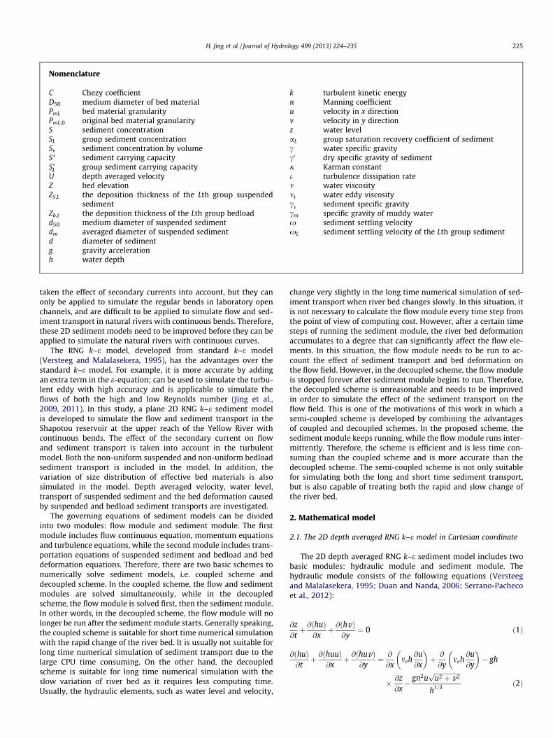
Fig. 1. The grid and control volume of finite volume method.

H. Jing et al. / Journal of Hydrology 499 (2013) 224–235 227

where U�

is the vertical mean velocity; D50 is the medium diameterof bed material; cs, cm is bulk densities of sediment and muddywater, respectively; xs is the group setting velocity. The units sys-tem adopted is kg, m and s.

The group sediment carrying capacity S�L is obtained by multi-plying S* with p�L (the graduation of group sediment carryingcapacity):

S�L ¼ p�LS� ð18Þ

and p�L can be calculated by Zhang (1988):

p�L ¼ wpL þ ð1�wÞp0bL ð19Þ

where PL is the graduation of suspended sediment at inlet; p0bL is re-lated to the graduation of bed material; w is the weight factor, andits value ranges from 0.62 to 0.85 when the river bed is silted; from0.64 to 0.86 when the river bed is scoured; and from 0.49 to 0.52when the river bed keeps the balance of erosion and deposition.

2.4. Sediment setting velocity

The sediment setting velocity is a very important parameter inthe sediment model. There are a lot of formulae to calculate sedi-ment setting velocity, among which the formula developed byZhang (1988) is one of the most representative formulae that aresuitable for the sediment in the Yellow River. According to Zhang(1988), the single grain sediment setting velocity in clean watercan be calculated as:

x0¼

125:6

cs�cc g d2

m for d60:1 mm

1:044ffiffiffiffiffiffiffiffiffiffiffiffiffics�c

c gdq

; for d P 4 mmffiffiffiffiffiffiffiffiffiffiffiffiffiffiffiffiffiffiffiffiffiffiffiffiffiffiffiffiffiffiffiffiffiffiffiffiffiffiffiffiffiffiffiffiffiffiffiffiffi13:95 m

d

� �2þ1:09cs�cc gd

q�C1

md ; for 0:1 mm< d<4 mm

8>>>><>>>>:

9>>>>=>>>>;ð20Þ

where x0 is the sediment setting velocity in clear water, d thediameter of single grain sediment.

The sediment concentration in the Yellow River is usuallyhigh, which will affect the sediment setting velocity. Therefore,the formula must be modified to take the effect of sediment con-centration into account. According to Zhang and Zhang (1992),the sediment setting velocity in muddy water can be estimatedas:

x ¼ x0 1� Sv

2:25ffiffiffiffiffiffiffid50

p !3:5

ð1� 1:25SvÞ

24

35 ð21Þ

where d50 is the medium diameter of a group of sediment.

2.5. Bedload sediment transport rate

Bedload transport rate is an important parameter that can becomputed as following (Dou et al., 1995):

gb;L ¼ K0csU

0U�

3

cs�cc gxLC2

0

ð22Þ

where K0 = 0.001; C0 = h1/6/(ng1/2); U0 ¼ U��Uc;U

�> Uc

0;U�6 Uc

(; Uc is the

incipient velocity of sediment, which can be calculated by:

Uc ¼ 0:265 ln11hD

� � ffiffiffiffiffiffiffiffiffiffiffiffiffiffiffiffiffiffiffiffiffiffiffiffiffiffiffiffiffiffiffiffiffiffiffiffiffiffiffiffiffiffiffiffiffiffiffiffiffiffiffiffiffics � c

cgdþ 0:19

ek þ ghddb50

sð23Þ

in which db50 is the medium bedload diameter;ek ¼ 2:56� 10�6 m3=s2; d ¼ 0:12� 10�6 m;D is roughness height ofrive bed and can be determined as:

D ¼0:5 mm; D50 � 0:5 mm;

D50;D50 > 0:5 mm:

�ð24Þ

2.6. Recovering saturation coefficient

Recovering saturation coefficient in (6) and (7) can be evaluatedby (Wei et al., 1997)

aL ¼0:001=x0:3

L ; SL � S�L0:001=x0:7

L ; SL < S�L

(ð25Þ

The above formula is used to calculate the recovering saturationcoefficient in (6) and (7).

3. Numerical methods

3.1. Discretization of the control equations

The general control Eq. (10) is discretized with finite volumemethod (FVM) (Versteeg and Malalasekera, 1995). The computa-tional domain is rectangular in the BFC system and can be easilydivided into a series of small rectangles, as shown in Fig. 1. Collo-cated grid system is adopted in this study. In order to avoid thecheckerboard pressure difference, momentum interpolation meth-od (Rhie and Chow, 1983) is used. The representative control vol-ume is DV and its centre is node P. The east, west, south andnorth faces of the control volume are e, w, s and n, respectively.The east, west, south and north neighbour nodes of P are E, W, Sand N, respectively. Integrating Eq. (10) over the control volumeDV yields:

ZDV

@

@tðhUÞdV þ

ZDV

1J@

@nðhUUÞdV þ

ZDV

1J@

@gðhVUÞdV

¼Z

DV

1J@

@nahCU

J@U@n

� �dV þ

ZDV

1J@

@gchCU

J@U@g

� �dV

þZ

DVSUðn;gÞdV ð26Þ

The first term (i.e. unsteady term, represented by It) on the left handside is discretized by the first order implicit scheme:

It¼:hPUP � h�PU

�P

DtJPDnDg ð27Þ

228 H. Jing et al. / Journal of Hydrology 499 (2013) 224–235

where Dt, Dn, Dg are time step, spatial steps in n and g directions,respectively. Subscript * represents the variable of the last timestep.

The second and third terms (i.e. convective terms, representedby IC) on the left hand side are discretized using an improvedQUICK scheme developed by Hayase et al. (1992). In this scheme,a deferred correction method presented by Khosla and Rubin(1974) is used to improve the QUICK scheme.

IC ¼ Ee � Ew þ En � Es ð28Þ

where

Ee ¼ ½jFe0j� UP þ18ð3UE � 2UP �UW Þ�

� �þ ½j

� Fe0j� UE þ18ð3UP � 2UE �UEEÞ�

� �ð29Þ

Ew ¼ ½jFw0j� UW þ18ð3UP � 2UW �UWWÞ�

� �þ ½j

� Fw0j� UE þ18ð3UW � 2UP �UEÞ�

� �ð30Þ

En ¼ ½jFn0j� UP þ18ð3UN � 2UP �USÞ�

� �þ ½j

� Fn0j� UN þ18ð3UP � 2UN �UNNÞ�

� �ð31Þ

Es ¼ ½jFs0j� US þ18ð3UP � 2US �USSÞ�

� �þ ½j

� Fs0j� UP þ18ð3US � 2UP �UNÞ�

� �ð32Þ

In which ½jFe;0j� ¼ maxðFe;0Þ; Fe ¼ ðhUDgÞe; Fn ¼ ðhVDnÞn.As a result, the scheme has not only the third order accuracy,

but is also diagonally dominant and can be easily programmed.The first and second terms on the right hand side (i.e. diffusion

terms, represented by ID) are discretized using the second ordercentral difference scheme.

ID ¼ DeðUE �UPÞ � DwðUP �UWÞ þ DnðUN �UPÞ � DsðUP

�USÞ ð33Þ

where

De ¼aCUh

J

� �e

DgðdnÞe

;Dn ¼cCUh

J

� �n

DnðdgÞn

:

The last term on the right hand side (the source term, representedby IS) can be dealt with using the following local linear method:

ISU ¼ ISUC þ ISUP UP ð34Þ

where ISUP 6 0. As for momentum equations, the source terms are asfollowing:

ISuC ¼�DnDg ghðznyg�zgynÞþ@

@nbCuh

J@u@g

� �þ @

@gbCuh

J@u@n

� �þ1

Juffiffifficpffiffiffiffiffiffiffiffiffiffiffiffiffiffiffiffi

u2þv2p @

@gðju�j�u/Þ

�

ISvC ¼�DnDg ghð�znxgþzgxnÞþ@

@nbCv h

J@v@g

� �þ @

@gbCv h

J@v@n

� �þ1

Jv ffiffifficpffiffiffiffiffiffiffiffiffiffiffiffiffiffiffiffiu2þv2p @

@gðj�uj�u/Þ

�

ISuP ¼ ISvP ¼ �gn2

ffiffiffiffiffiffiffiffiffiffiffiffiffiffiffiffiu2 þ v2p

h1=3 JPDnDg:

The discretized equation of the general governing Eq. (10) using theabove discretized scheme is as following:

aPUP ¼ aEUE þ aWUW þ aNUN þ aSUS þ ISUC þ S�ad ð35Þ

where

aE ¼ De þ ½j � Fe;0j�; aW ¼ Dw þ ½jFw;0j�; aN ¼ Dn þ ½j � Fn;0j�; aS

¼ Ds þ ½jFs;0j�;

aP ¼ aE þ aW þ aN þ aS þ Fe � Fw þ Fn � Fs þ a�P � ISUP ; b

¼ a�PU�P þ ISUC ;

a�P ¼h�PDt

JPDnDg; S�ad ¼ S�ad

� �e þ S�ad

� �w þ S�ad

� �n þ S�ad

� �s;

S�ad

� �e ¼

18ð3UE � 2UP �UWÞ�½jFe0j� þ 1

8ð3UP � 2UE �UEEÞ�½j

� Fe0j�;

S�ad

� �w ¼

18ð3UP � 2UW �UWWÞ�½jFw0j� þ 1

8ð3UW � 2UP �UEÞ�½j

� Fw0j�;

S�ad

� �n ¼

18ð3UN � 2UP �USÞ�½jFn0j� þ 1

8ð3UP � 2UN �UNNÞ�½j

� Fn0j�;

S�ad

� �s ¼

18ð3UP � 2US �USSÞ�½jFs0j� þ

18ð3US � 2UP �UNÞ�½j � Fs0j�:

Collocated grids SIMPLEC algorithm in body fitted coordinatesystem (Van Doormaal and Raithby, 1984) is used to solvethe coupled problem of water level and velocities. The discret-ized equations are five-diagonal, which can be solved using tri-diagonal matrix algorithm (TDMA) (Versteeg and Malalasekera,1995).

3.2. Semi-coupled algorithm for sediment model

In this study, a semi-coupled algorithm is developed by com-bining the advantages of coupled and decoupled schemes. In theprocess of long time simulation of sediment transport when riverbed changes slowly, the bed elevation change each time step hasminimal impacts on flow field, therefore, it is unnecessary toupdate the hydraulic elements each time step. Thus, in order to re-duce the computational cost, the hydraulic module runs intermit-tently while the sediment module keeps running all the time. Inthe semi-coupled scheme, after the sediment module starts torun, the hydraulic module will stop running for a certain numberof time steps (for example, 1000–5000 time steps), then it willrun again. After running for certain time steps (such as 60–120time steps) to update the hydraulic elements, it will then stoprunning. The process is repeated until the required accuracy isreached.

Let t be simulating time, t0_flow the initial simulating time forthe flow module, t1_flow the flow module working time each time,t2_flow the time interval between two adjacent times when flowmodule is started, t_max the required simulating time, the proce-dure of this semi-coupled scheme is detailed as following:

Algorithm of semi-coupled scheme:

� Step 1. If t 6 t0_flow, only the hydraulic module is running.� Step 2. If t0_flow < t < t_max, the sediment module is running.� Step 3. If t0_flow < t < t_max, and mod (t, t2_flow) < t1_flow, the

flow and sediment modules are running together; otherwise,only the sediment module is running.� Step 4. If t > t_max, stop.

H. Jing et al. / Journal of Hydrology 499 (2013) 224–235 229

where mod is a function which means modulus and mod (t,t2_flow) is the remainder when t is divided by t2_flow. In this study,time step dt = 12s, t0_flow = 5h, t1_flow = 1 h, t2_flow = 12 h.Numerical experiments indicate that the computational time ofthe semi-coupled scheme is about 60% of the coupled scheme.

3.3. Boundary and initial conditions

We choose two adjacent field measurements to verify the sed-iment model. The field measurements were conducted on Decem-ber 6, 2008 and on July 17, 2009, respectively. The time intervalbetween the two measurements is 203 days. Water dischargeand sediment concentration are given at the inlet based on valuesinterpolated by field data measured on December 6, 2008 and onJuly 17, 2009. The turbulence kinetic energy (k) and its dissipationrate (e) at the inlet are calculated using empirical formulae (Rodi,1993). On the water outlet boundary, water level specified setbased on values by interpolating the field data measured onDecember 6, 2008 and on July 17, 2009. Other variables are dealtwith fully developed condition. On the wall boundary, no-slipboundary condition is applied. The velocity parallel to the riverbank at the first cell is estimated using standard wall function(Guo et al., 2008).

In order to study the flow and sediment transport in the studiedreach, four cases are set based on discharge and sediment concen-tration at the inlet. The boundary conditions of the four cases arepresented in Table 1. Case 1 is set according to the field measureddata on December 6, 2008, while Case 2 is set according to the datameasured on July 17, 2009. Case 3 and Case 4 are set according tothe hydrological data in the past years. Cases 1 and 4 representsthe hydraulic conditions of the dry and flood seasons, respectively,while Cases 2 and 3 represents the hydraulic condition of the wetseason.

The initial values are based on field measured data on Decem-ber 6, 2008, including the position of cross-sections, water level,maximum water depth, average water depth, river width, averagevelocity of 14 cross-sections (see Table 2). The initial water level ateach grid is set as the same as the water level at the outlet. u, v andSL at each grid are set as zero, except for that at the grids at the in-let. However, k and e cannot be set as zero, otherwise, the simula-tion process will stop unexpected or be unstable. In thesimulations, the initial values of k and e are set as 0.1 m2/s2 and0.0001 m2/s2, respectively, based on the authors’ experience.

The suspended and bedload sediment on the inlet section is di-vided into three groups with the medium diameter being0.0249 mm and 10 mm, respectively. The representative diametersand related percentage for both suspended and bedload sedimentare listed in Table 3. The bed material is divided into six groups,whose representative diameters and their percent content are pre-sented in Table 3. The initial percentage contents of the suspendedand bedload are set as the same as the values at the inlet. Somerepresentative diameters of the initial bed material of the wholereach are: d50 = 10 mm, dm = 15.5 mm, d25 = 1 mm, d35 = 4 mm,d75 = 20 mm, d90 = 70 mm and d95 = 100 mm, where dm is the mean

Table 1Boundary conditions of four cases.

Cases Inlet Outlet

Q (m3/s) U (m/s) S (kg/m3) k (m2/s2) e (m2/s3) z (m)

Case 1 513.50 1.0398 0.51 0.0121 0.0005 1239.68Case 2 930.00 1.5405 3.53 0.0269 0.0013 1240.65Case 3 1500.00 1.8098 10 0.0378 0.0016 1241.50Case 4 2000.00 2.0579 20 0.0492 0.0020 1242.00

diameter, da is the sediment diameter that a% is less than that inthe size gradation curve (a = 25,35,50,75,90,95).

3.4. Mesh generation

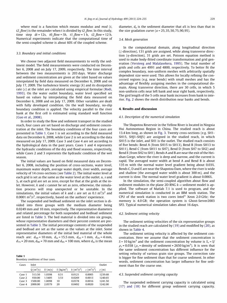
In the computational domain, along longitudinal direction(n-direction), 131 grids are assigned, while along transverse direc-tion (g-direction), 31 grids are set. Poisson equation method isused to make body-fitted coordinate transformation and grid gen-eration (Versteeg and Malalasekera, 1995). The total number ofgrids and cells are 4991 and 4800, respectively. To better fit thecomplex boundary, non-uniform meshes with arbitrarily spatiallydependent size were used. This allows for locally refining the con-cerned regions (e.g. near bends) with small meshes and has theadvantage of flexibly assigning meshes in the computational do-main. Along transverse direction, there are 30 cells, in which 5non-uniform cells near left bank and near right bank, respectively.The gird length of the 5 cells near bank increases from bank to inte-rior. Fig. 2 shows the mesh distribution near banks and bends.

4. Results and discussion

4.1. Description of the numerical simulation

The Shapotou Reservoir in the Yellow River is located in NingxiaHui Autonomous Region in China. The studied reach is about13.4 km long, as shown in Fig. 3. Twenty cross-sections (e.g. SH1-SH15, SHJ1-SHJ5) are assigned in the studied reach, in whichSH15 is the inlet, and SH1 is the outlet. The studied reach consistsof five bends: Bend A (from SH15 to SH13), Bend B (from SH13 toSH11), Bend C (from SH11 to SH7), Bend D (from SH7 to SH2) andBend E (from SH2 to SH1). Bends A and B are near the exit of the Hei-shan Gorge, where the river is deep and narrow, and the current israpid. The averaged water width at bend A and Bend B is about135 m with the normal water level gradient being about 0.03%.Bends C, D and E are near the Shapotou Dam, where the river is wideand shallow (the averaged water width is about 300 m), and thecurrent is slow. The normal water level gradient is about 0.006%.

In the simulation, the semi-coupled algorithm about flow andsediment modules in the plane 2D RNG k–e sediment model is ap-plied. The software of Matlab 7.1 is used to program, and thenumerical simulation is conducted in an IBM work station. TheCPU of the work station is two cores Intel� Xeon 2.0 GHz; thememory is 4.0 GB; the operation system is Ghost-Server2003SP2. Typical numerical simulation takes about 16 days.

4.2. Sediment setting velocity

The sediment setting velocities of the six representative groupsin the studied reach are calculated by (19) and modified by (20), asshown in Table 4.

The sediment setting velocity is affected by the sediment con-centration. Here we assume that the sediment concentration isS = 10 kg/m3 and the sediment concentration by volume is Sv = S/qs = 0.038 (qs = density of sediment = 2650 kg/m3). It is seen thatthe same sediment concentration has different influence for thesetting velocity of various grain size groups. The correction rateis bigger for fine sediment than that for coarse sediment. In otherwords, sediment concentration has larger influence for fine sedi-ment than for the coarse one.

4.3. Suspended sediment carrying capacity

The suspended sediment carrying capacity is calculated using(17) and (18) for different group sediment carrying capacity.

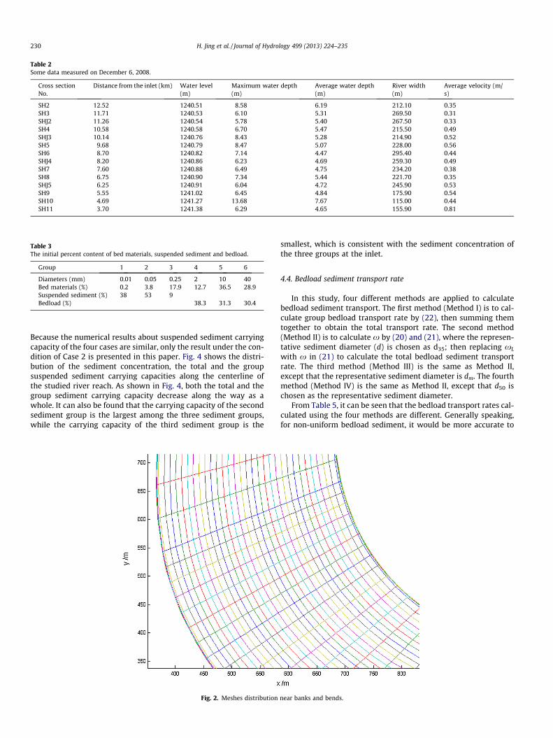
Table 2Some data measured on December 6, 2008.

Cross sectionNo.

Distance from the inlet (km) Water level(m)

Maximum water depth(m)

Average water depth(m)

River width(m)

Average velocity (m/s)

SH2 12.52 1240.51 8.58 6.19 212.10 0.35SH3 11.71 1240.53 6.10 5.31 269.50 0.31SHJ2 11.26 1240.54 5.78 5.40 267.50 0.33SH4 10.58 1240.58 6.70 5.47 215.50 0.49SHJ3 10.14 1240.76 8.43 5.28 214.90 0.52SH5 9.68 1240.79 8.47 5.07 228.00 0.56SH6 8.70 1240.82 7.14 4.47 295.40 0.44SHJ4 8.20 1240.86 6.23 4.69 259.30 0.49SH7 7.60 1240.88 6.49 4.75 234.20 0.38SH8 6.75 1240.90 7.34 5.44 221.70 0.35SHJ5 6.25 1240.91 6.04 4.72 245.90 0.53SH9 5.55 1241.02 6.45 4.84 175.90 0.54SH10 4.69 1241.27 13.68 7.67 115.00 0.44SH11 3.70 1241.38 6.29 4.65 155.90 0.81

Table 3The initial percent content of bed materials, suspended sediment and bedload.

Group 1 2 3 4 5 6

Diameters (mm) 0.01 0.05 0.25 2 10 40Bed materials (%) 0.2 3.8 17.9 12.7 36.5 28.9Suspended sediment (%) 38 53 9Bedload (%) 38.3 31.3 30.4

230 H. Jing et al. / Journal of Hydrology 499 (2013) 224–235

Because the numerical results about suspended sediment carryingcapacity of the four cases are similar, only the result under the con-dition of Case 2 is presented in this paper. Fig. 4 shows the distri-bution of the sediment concentration, the total and the groupsuspended sediment carrying capacities along the centerline ofthe studied river reach. As shown in Fig. 4, both the total and thegroup sediment carrying capacity decrease along the way as awhole. It can also be found that the carrying capacity of the secondsediment group is the largest among the three sediment groups,while the carrying capacity of the third sediment group is the

Fig. 2. Meshes distribution

smallest, which is consistent with the sediment concentration ofthe three groups at the inlet.

4.4. Bedload sediment transport rate

In this study, four different methods are applied to calculatebedload sediment transport. The first method (Method I) is to cal-culate group bedload transport rate by (22), then summing themtogether to obtain the total transport rate. The second method(Method II) is to calculate x by (20) and (21), where the represen-tative sediment diameter (d) is chosen as d35; then replacing xL

with x in (21) to calculate the total bedload sediment transportrate. The third method (Method III) is the same as Method II,except that the representative sediment diameter is dm. The fourthmethod (Method IV) is the same as Method II, except that d50 ischosen as the representative sediment diameter.

From Table 5, it can be seen that the bedload transport rates cal-culated using the four methods are different. Generally speaking,for non-uniform bedload sediment, it would be more accurate to

near banks and bends.

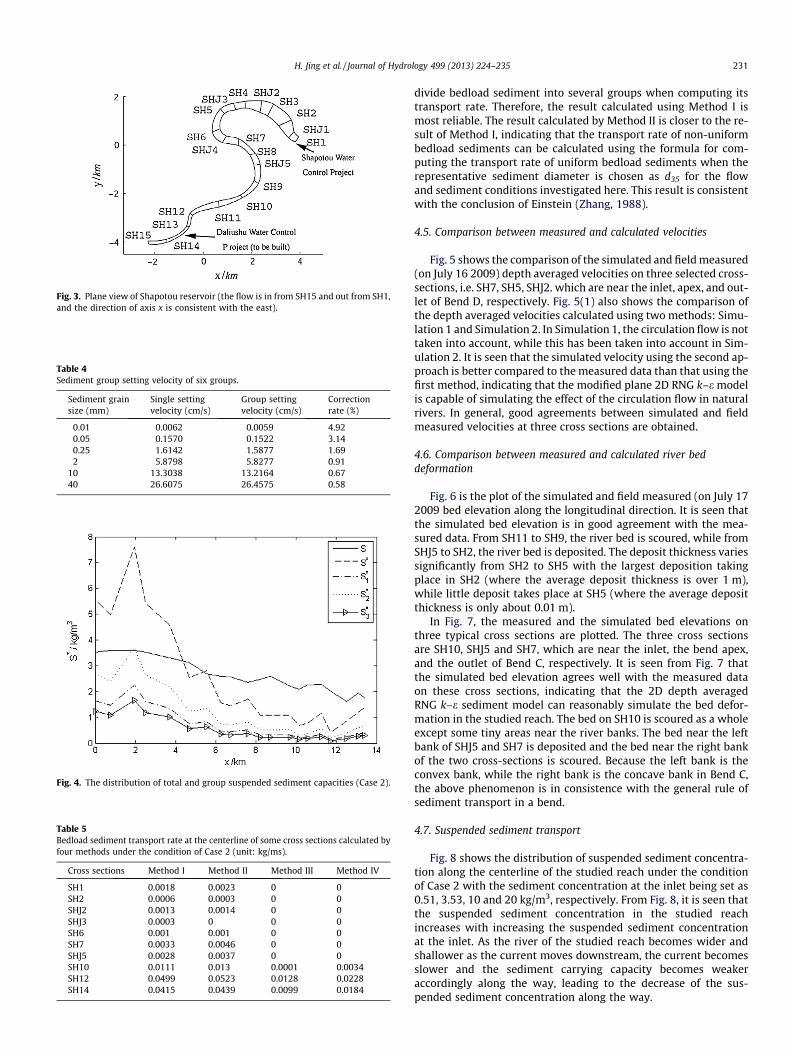
Fig. 3. Plane view of Shapotou reservoir (the flow is in from SH15 and out from SH1,and the direction of axis x is consistent with the east).

Table 4Sediment group setting velocity of six groups.

Sediment grainsize (mm)

Single settingvelocity (cm/s)

Group settingvelocity (cm/s)

Correctionrate (%)

0.01 0.0062 0.0059 4.920.05 0.1570 0.1522 3.140.25 1.6142 1.5877 1.692 5.8798 5.8277 0.91

10 13.3038 13.2164 0.6740 26.6075 26.4575 0.58

Fig. 4. The distribution of total and group suspended sediment capacities (Case 2).

Table 5Bedload sediment transport rate at the centerline of some cross sections calculated byfour methods under the condition of Case 2 (unit: kg/ms).

Cross sections Method I Method II Method III Method IV

SH1 0.0018 0.0023 0 0SH2 0.0006 0.0003 0 0SHJ2 0.0013 0.0014 0 0SHJ3 0.0003 0 0 0SH6 0.001 0.001 0 0SH7 0.0033 0.0046 0 0SHJ5 0.0028 0.0037 0 0SH10 0.0111 0.013 0.0001 0.0034SH12 0.0499 0.0523 0.0128 0.0228SH14 0.0415 0.0439 0.0099 0.0184

H. Jing et al. / Journal of Hydrology 499 (2013) 224–235 231

divide bedload sediment into several groups when computing itstransport rate. Therefore, the result calculated using Method I ismost reliable. The result calculated by Method II is closer to the re-sult of Method I, indicating that the transport rate of non-uniformbedload sediments can be calculated using the formula for com-puting the transport rate of uniform bedload sediments when therepresentative sediment diameter is chosen as d35 for the flowand sediment conditions investigated here. This result is consistentwith the conclusion of Einstein (Zhang, 1988).

4.5. Comparison between measured and calculated velocities

Fig. 5 shows the comparison of the simulated and field measured(on July 16 2009) depth averaged velocities on three selected cross-sections, i.e. SH7, SH5, SHJ2. which are near the inlet, apex, and out-let of Bend D, respectively. Fig. 5(1) also shows the comparison ofthe depth averaged velocities calculated using two methods: Simu-lation 1 and Simulation 2. In Simulation 1, the circulation flow is nottaken into account, while this has been taken into account in Sim-ulation 2. It is seen that the simulated velocity using the second ap-proach is better compared to the measured data than that using thefirst method, indicating that the modified plane 2D RNG k–e modelis capable of simulating the effect of the circulation flow in naturalrivers. In general, good agreements between simulated and fieldmeasured velocities at three cross sections are obtained.

4.6. Comparison between measured and calculated river beddeformation

Fig. 6 is the plot of the simulated and field measured (on July 172009 bed elevation along the longitudinal direction. It is seen thatthe simulated bed elevation is in good agreement with the mea-sured data. From SH11 to SH9, the river bed is scoured, while fromSHJ5 to SH2, the river bed is deposited. The deposit thickness variessignificantly from SH2 to SH5 with the largest deposition takingplace in SH2 (where the average deposit thickness is over 1 m),while little deposit takes place at SH5 (where the average depositthickness is only about 0.01 m).

In Fig. 7, the measured and the simulated bed elevations onthree typical cross sections are plotted. The three cross sectionsare SH10, SHJ5 and SH7, which are near the inlet, the bend apex,and the outlet of Bend C, respectively. It is seen from Fig. 7 thatthe simulated bed elevation agrees well with the measured dataon these cross sections, indicating that the 2D depth averagedRNG k–e sediment model can reasonably simulate the bed defor-mation in the studied reach. The bed on SH10 is scoured as a wholeexcept some tiny areas near the river banks. The bed near the leftbank of SHJ5 and SH7 is deposited and the bed near the right bankof the two cross-sections is scoured. Because the left bank is theconvex bank, while the right bank is the concave bank in Bend C,the above phenomenon is in consistence with the general rule ofsediment transport in a bend.

4.7. Suspended sediment transport

Fig. 8 shows the distribution of suspended sediment concentra-tion along the centerline of the studied reach under the conditionof Case 2 with the sediment concentration at the inlet being set as0.51, 3.53, 10 and 20 kg/m3, respectively. From Fig. 8, it is seen thatthe suspended sediment concentration in the studied reachincreases with increasing the suspended sediment concentrationat the inlet. As the river of the studied reach becomes wider andshallower as the current moves downstream, the current becomesslower and the sediment carrying capacity becomes weakeraccordingly along the way, leading to the decrease of the sus-pended sediment concentration along the way.

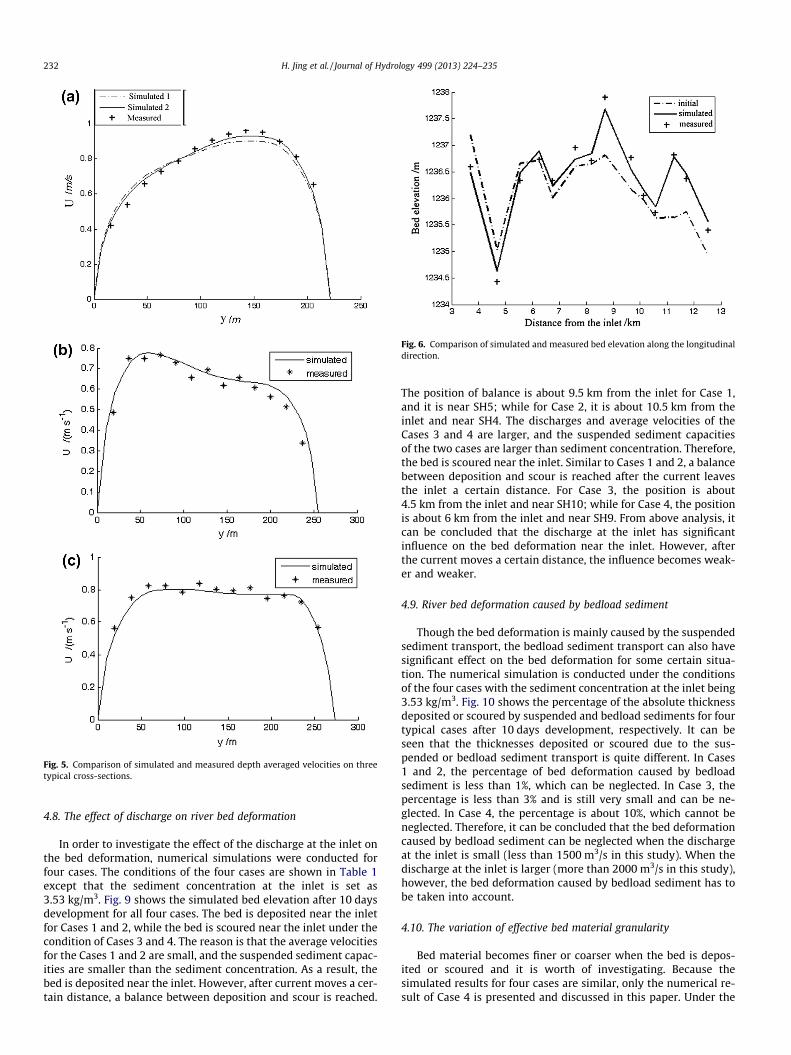
Fig. 5. Comparison of simulated and measured depth averaged velocities on threetypical cross-sections.

Fig. 6. Comparison of simulated and measured bed elevation along the longitudinaldirection.

232 H. Jing et al. / Journal of Hydrology 499 (2013) 224–235

4.8. The effect of discharge on river bed deformation

In order to investigate the effect of the discharge at the inlet onthe bed deformation, numerical simulations were conducted forfour cases. The conditions of the four cases are shown in Table 1except that the sediment concentration at the inlet is set as3.53 kg/m3. Fig. 9 shows the simulated bed elevation after 10 daysdevelopment for all four cases. The bed is deposited near the inletfor Cases 1 and 2, while the bed is scoured near the inlet under thecondition of Cases 3 and 4. The reason is that the average velocitiesfor the Cases 1 and 2 are small, and the suspended sediment capac-ities are smaller than the sediment concentration. As a result, thebed is deposited near the inlet. However, after current moves a cer-tain distance, a balance between deposition and scour is reached.

The position of balance is about 9.5 km from the inlet for Case 1,and it is near SH5; while for Case 2, it is about 10.5 km from theinlet and near SH4. The discharges and average velocities of theCases 3 and 4 are larger, and the suspended sediment capacitiesof the two cases are larger than sediment concentration. Therefore,the bed is scoured near the inlet. Similar to Cases 1 and 2, a balancebetween deposition and scour is reached after the current leavesthe inlet a certain distance. For Case 3, the position is about4.5 km from the inlet and near SH10; while for Case 4, the positionis about 6 km from the inlet and near SH9. From above analysis, itcan be concluded that the discharge at the inlet has significantinfluence on the bed deformation near the inlet. However, afterthe current moves a certain distance, the influence becomes weak-er and weaker.

4.9. River bed deformation caused by bedload sediment

Though the bed deformation is mainly caused by the suspendedsediment transport, the bedload sediment transport can also havesignificant effect on the bed deformation for some certain situa-tion. The numerical simulation is conducted under the conditionsof the four cases with the sediment concentration at the inlet being3.53 kg/m3. Fig. 10 shows the percentage of the absolute thicknessdeposited or scoured by suspended and bedload sediments for fourtypical cases after 10 days development, respectively. It can beseen that the thicknesses deposited or scoured due to the sus-pended or bedload sediment transport is quite different. In Cases1 and 2, the percentage of bed deformation caused by bedloadsediment is less than 1%, which can be neglected. In Case 3, thepercentage is less than 3% and is still very small and can be ne-glected. In Case 4, the percentage is about 10%, which cannot beneglected. Therefore, it can be concluded that the bed deformationcaused by bedload sediment can be neglected when the dischargeat the inlet is small (less than 1500 m3/s in this study). When thedischarge at the inlet is larger (more than 2000 m3/s in this study),however, the bed deformation caused by bedload sediment has tobe taken into account.

4.10. The variation of effective bed material granularity

Bed material becomes finer or coarser when the bed is depos-ited or scoured and it is worth of investigating. Because thesimulated results for four cases are similar, only the numerical re-sult of Case 4 is presented and discussed in this paper. Under the

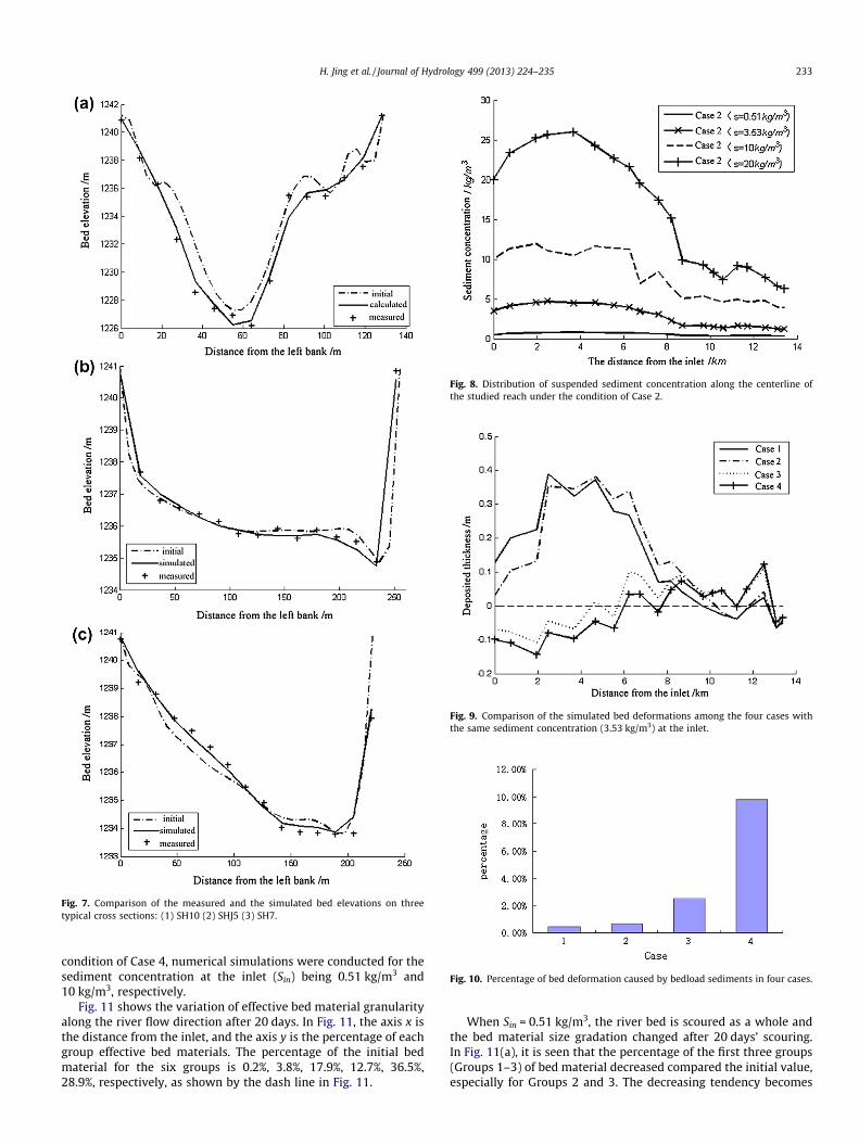
Fig. 7. Comparison of the measured and the simulated bed elevations on threetypical cross sections: (1) SH10 (2) SHJ5 (3) SH7.

Fig. 8. Distribution of suspended sediment concentration along the centerline ofthe studied reach under the condition of Case 2.

Fig. 9. Comparison of the simulated bed deformations among the four cases withthe same sediment concentration (3.53 kg/m3) at the inlet.

Fig. 10. Percentage of bed deformation caused by bedload sediments in four cases.

H. Jing et al. / Journal of Hydrology 499 (2013) 224–235 233

condition of Case 4, numerical simulations were conducted for thesediment concentration at the inlet (Sin) being 0.51 kg/m3 and10 kg/m3, respectively.

Fig. 11 shows the variation of effective bed material granularityalong the river flow direction after 20 days. In Fig. 11, the axis x isthe distance from the inlet, and the axis y is the percentage of eachgroup effective bed materials. The percentage of the initial bedmaterial for the six groups is 0.2%, 3.8%, 17.9%, 12.7%, 36.5%,28.9%, respectively, as shown by the dash line in Fig. 11.

When Sin = 0.51 kg/m3, the river bed is scoured as a whole andthe bed material size gradation changed after 20 days’ scouring.In Fig. 11(a), it is seen that the percentage of the first three groups(Groups 1–3) of bed material decreased compared the initial value,especially for Groups 2 and 3. The decreasing tendency becomes

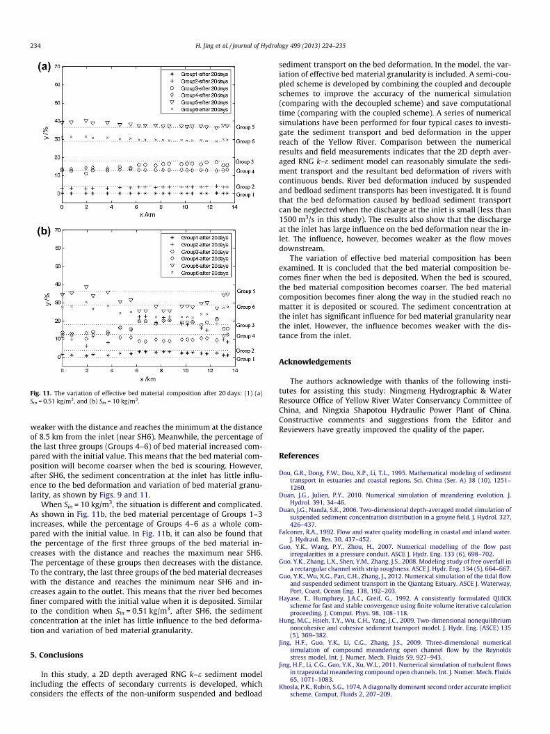
Fig. 11. The variation of effective bed material composition after 20 days: (1) (a)Sin = 0.51 kg/m3, and (b) Sin = 10 kg/m3.

234 H. Jing et al. / Journal of Hydrology 499 (2013) 224–235

weaker with the distance and reaches the minimum at the distanceof 8.5 km from the inlet (near SH6). Meanwhile, the percentage ofthe last three groups (Groups 4–6) of bed material increased com-pared with the initial value. This means that the bed material com-position will become coarser when the bed is scouring. However,after SH6, the sediment concentration at the inlet has little influ-ence to the bed deformation and variation of bed material granu-larity, as shown by Figs. 9 and 11.

When Sin = 10 kg/m3, the situation is different and complicated.As shown in Fig. 11b, the bed material percentage of Groups 1–3increases, while the percentage of Groups 4–6 as a whole com-pared with the initial value. In Fig. 11b, it can also be found thatthe percentage of the first three groups of the bed material in-creases with the distance and reaches the maximum near SH6.The percentage of these groups then decreases with the distance.To the contrary, the last three groups of the bed material decreaseswith the distance and reaches the minimum near SH6 and in-creases again to the outlet. This means that the river bed becomesfiner compared with the initial value when it is deposited. Similarto the condition when Sin = 0.51 kg/m3, after SH6, the sedimentconcentration at the inlet has little influence to the bed deforma-tion and variation of bed material granularity.

5. Conclusions

In this study, a 2D depth averaged RNG k–e sediment modelincluding the effects of secondary currents is developed, whichconsiders the effects of the non-uniform suspended and bedload

sediment transport on the bed deformation. In the model, the var-iation of effective bed material granularity is included. A semi-cou-pled scheme is developed by combining the coupled and decoupleschemes to improve the accuracy of the numerical simulation(comparing with the decoupled scheme) and save computationaltime (comparing with the coupled scheme). A series of numericalsimulations have been performed for four typical cases to investi-gate the sediment transport and bed deformation in the upperreach of the Yellow River. Comparison between the numericalresults and field measurements indicates that the 2D depth aver-aged RNG k–e sediment model can reasonably simulate the sedi-ment transport and the resultant bed deformation of rivers withcontinuous bends. River bed deformation induced by suspendedand bedload sediment transports has been investigated. It is foundthat the bed deformation caused by bedload sediment transportcan be neglected when the discharge at the inlet is small (less than1500 m3/s in this study). The results also show that the dischargeat the inlet has large influence on the bed deformation near the in-let. The influence, however, becomes weaker as the flow movesdownstream.

The variation of effective bed material composition has beenexamined. It is concluded that the bed material composition be-comes finer when the bed is deposited. When the bed is scoured,the bed material composition becomes coarser. The bed materialcomposition becomes finer along the way in the studied reach nomatter it is deposited or scoured. The sediment concentration atthe inlet has significant influence for bed material granularity nearthe inlet. However, the influence becomes weaker with the dis-tance from the inlet.

Acknowledgements

The authors acknowledge with thanks of the following insti-tutes for assisting this study: Ningmeng Hydrographic & WaterResource Office of Yellow River Water Conservancy Committee ofChina, and Ningxia Shapotou Hydraulic Power Plant of China.Constructive comments and suggestions from the Editor andReviewers have greatly improved the quality of the paper.

References

Dou, G.R., Dong, F.W., Dou, X.P., Li, T.L., 1995. Mathematical modeling of sedimenttransport in estuaries and coastal regions. Sci. China (Ser. A) 38 (10), 1251–1260.

Duan, J.G., Julien, P.Y., 2010. Numerical simulation of meandering evolution. J.Hydrol. 391, 34–46.

Duan, J.G., Nanda, S.K., 2006. Two-dimensional depth-averaged model simulation ofsuspended sediment concentration distribution in a groyne field. J. Hydrol. 327,426–437.

Falconer, R.A., 1992. Flow and water quality modelling in coastal and inland water.J. Hydraul. Res. 30, 437–452.

Guo, Y.K., Wang, P.Y., Zhou, H., 2007. Numerical modelling of the flow pastirregularities in a pressure conduit. ASCE J. Hydr. Eng. 133 (6), 698–702.

Guo, Y.K., Zhang, L.X., Shen, Y.M., Zhang, J.S., 2008. Modeling study of free overfall ina rectangular channel with strip roughness. ASCE J. Hydr. Eng. 134 (5), 664–667.

Guo, Y.K., Wu, X.G., Pan, C.H., Zhang, J., 2012. Numerical simulation of the tidal flowand suspended sediment transport in the Qiantang Estuary. ASCE J. Waterway,Port, Coast. Ocean Eng. 138, 192–203.

Hayase, T., Humphrey, J.A.C., Greif, G., 1992. A consistently formulated QUICKscheme for fast and stable convergence using finite volume iterative calculationproceeding. J. Comput. Phys. 98, 108–118.

Hung, M.C., Hsieh, T.Y., Wu, C.H., Yang, J.C., 2009. Two-dimensional nonequilibriumnoncohesive and cohesive sediment transport model. J. Hydr. Eng. (ASCE) 135(5), 369–382.

Jing, H.F., Guo, Y.K., Li, C.G., Zhang, J.S., 2009. Three-dimensional numericalsimulation of compound meandering open channel flow by the Reynoldsstress model. Int. J. Numer. Mech. Fluids 59, 927–943.

Jing, H.F., Li, C.G., Guo, Y.K., Xu, W.L., 2011. Numerical simulation of turbulent flowsin trapezoidal meandering compound open channels. Int. J. Numer. Mech. Fluids65, 1071–1083.

Khosla, P.K., Rubin, S.G., 1974. A diagonally dominant second order accurate implicitscheme. Comput. Fluids 2, 207–209.

H. Jing et al. / Journal of Hydrology 499 (2013) 224–235 235

Li, S.S., Millar, R.G., 2011. A two-dimensional morphodynamic model of gravel-bedriver with floodplain vegetation. Earth Surf. Process Landf. 36 (2), 190–202.

Lien, H.C., Hsieh, T.Y., Yang, J.C., Yeh, K.C., 1999. Bend-flow simulation using 2Ddepth-averaged model. ASCE J. Hydr. Eng. 125, 1097–1108.

Nagata, N., Hosoda, T., Muramoto, Y., 2000. Numerical analysis of river channelprocesses with bank erosion. ASCE J. Hydr. Eng. 126 (4), 243–252.

Rhie, C.M., Chow, W.L., 1983. A numerical study of the turbulent flow past anisolated airfoil with trailing edge separation. AAIA J. 21, 1525–1532.

Rodi, W., 1993. Turbulence Models and their Application in Hydraulics: A State-of-the-Art Review, third ed., Balkema, Rotterdam, the Netherlands.

Serrano-Pacheco, A., Murillo, J., Garcia-Navarro, P., 2012. Finite volumes for 2Dshallow-water flow with bed-load transport on unstructured grids. J. Hydraul.Res. 50 (2), 154–163.

Van Doormaal, J.P., Raithby, G.D., 1984. Enhancement of SIMPLE method forpredicting incompressible fluid flows. Numer. Heat Trans. 7 (2), 147–163.

Versteeg, H.K., Malalasekera, W., 1995. An Introduction to Computational FluidDynamics. Addison Wesley Longman Limited, England.

Wei, Z.L., Zhao, L.K., Fu, X.P., 1997. Research on mathematical model for sediment inyellow river. J. Wuhan Univer. Hydro. Electr. Eng. 30 (5), 21–25.

Yakhot, V., Orzag, S.A., 1986. Renomalization group analysis of turbulence: basictheory. J. Scient Comput. 1, 3–11.

Zhang, R.J., 1988. River Sediment Dynamics, second ed. Water Conserversy andHydropower of China, Beijing.

Zhang, H.W., Zhang, Q., 1992. Formula of sediment carrying capacity of the yellowriver. Yellow River 11, 6–9.