MODELLING THE BEHAVIOUR OF SHINGLE BEACHES: A REVIEW › geography › researchprojects › BAR... · beaches is highly varied, some consisting almost entirely of shingle whilst others

MODELLING THE BEHAVIOUR OF SHINGLE BEACHES: A REVIEW

Compiled by T. Watt, edited by C. Moses

1 Introduction............................................................................................................................2

1.1 What is a Model ? ......................................................................................................3 2 Mixed shingle beach research ..........................................................................................3

2.1 Introduction ................................................................................................................3 2.2 Background................................................................................................................3 2.3 Beach permeability and hydraulic conductivity ..........................................................4 2.4 Swash zone dynamics ...............................................................................................5 2.5 Wave Reflection.........................................................................................................7 2.6 Threshold of movement .............................................................................................8

3 Predicting and Modelling mixed shingle beaches .............................................................9 3.1 Existing predictive methods .......................................................................................9 3.2 Physical models .........................................................................................................9

3.2.1 Numerical models .............................................................................................10 3.2.2 Longshore transport models .............................................................................11

4 Existing models for mixed shingle beaches ....................................................................11 4.1 Litpack: An integrated modelling system .................................................................11

4.1.1 Modelling applications ......................................................................................12 4.1.2 LITDRIFT – longshore current and littoral drift .................................................12

4.2 Cross shore profile development .............................................................................13 4.2.1 The Beach profile prediction model SHINGLE .................................................13 4.2.2 Model test .........................................................................................................15 4.2.3 Building the model ............................................................................................16 4.2.4 Model operation ................................................................................................17

5 References......................................................................................................................19

BAR Phase I, February 2003 – January 2005 Science Report: Modelling the behaviour of shingle beaches: a review

1 Introduction In today’s environment of global warming and sea level rise, coastal erosion is a well-known phrase and an all too common phenomena. Many of the world’s coastlines are eroding and conflicting demands for economic development, recreation and conservation place huge pressures on these sensitive and ultimately vulnerable environments. As populations continue to expand, pressures on the coastline are only likely to increase. These factors, in combination with changing wave and climatic conditions, will lead to increased rates of coastal erosion. The majority of existing research on beach processes and morphodynamics has concentrated upon sandy beaches, however mixed shingle beaches1 are increasingly seen as important to both coastal managers and coastal engineers. Mixed shingle beaches exist in a variety of forms, from barrier ridges to cuspate forelands and the composition of these beaches is highly varied, some consisting almost entirely of shingle whilst others have a high sand content within the shingle interstitial matrix. Particle size distribution also varies, with D50 values ranging from between 10mm to 30mm depending upon the coastal setting. Such diversity of form is of obvious importance when considering the behaviour and response of a mixed shingle beach and the need to successfully develop and monitor coastal protection schemes. Mixed shingle beaches are one of the most effective natural sea defences and provide an attractive, practical means of coastal protection. Capable of dissipating in excess of 90% of all incident wave energy the beaches respond rapidly to varying wave conditions, reacting even to individual waves in a train (Powell 1990). Although an efficient form of coastal protection, these beaches in common with any other type of beach will suffer erosion under ‘extreme conditions’ of combined high water levels and storm waves. The response, dependent upon the wave conditions acting on the beach, includes crest erosion and the eroded material is either pushed up the beach face to form a berm or drawn down offshore toward the beach toe. If crest erosion is sufficiently severe the beach will reach a point at which it can no longer absorb wave energy and breaching will occur, at this point the beach can be considered to have failed as a coastal protection system. Continued damage may eventually lead to changes within the dominant hydraulic processes, making natural recovery impossible and landward retreat of the beach inevitable. Consequently predicting the evolution of mixed shingle beaches and identifying and calculating patterns of accumulation or loss of sediment are particularly important issues. Prevention of beach failure depends upon correct, accurate assessment and maintenance of the beach structure, the beach must be maintained to a level above that of the calculated failure threshold. In today’s climate of increased environmental awareness, this topic is vital due to the increased use of “soft engineering” methods for beach management, coastal protection and flood defence. These techniques rely heavily on the provision and maintenance of adequate beach levels and the use of predictive modelling can be essential in determining the dimensions and predicting the behaviour of beach recharge schemes. Mixed shingle beach systems can be considered as a combination of complex, poorly understood component subsystems and the best way to gain insights into their structure, organisation and functioning is to employ the use of models (Lakhan 1986). Models are able to provide insights into the complexities of beach systems, involving the interrelationships between and among the many variables and parameters. Such features

1 Composite sand and shingle beaches with particle sizes ranging from less than 1mm for sand up to 50 and even 100mm for gravels and cobbles.


2

make them indispensable in our efforts to monitor, manage, control and develop the coastal system and its interrelated resources.

1.1 What is a Model ? The term model can be employed in several different ways and there are various classes of models and types of modeller (for example Keulegan and Krumbein 1949, Brunn 1954, Krumbien 1968, Rivet 1972, Swart 1974 – 76, Dean 1977, Hughes and Chiu 1978, Vellinga 1984, Fox 1985, Powell 1986, Van der Meer 1988). Models can be considered as imitations or approximations made upon the real world, even at their most complex models are not reality and at best can only be considered as a representation of such. However, while models may only be a generalisation or simplification of a system, they can provide valuable insight for experimentation, analysis and prediction. For practical purposes many types of model representation are used, and models can be classified in several ways. Of the wide range of techniques available and employed in the study of natural systems, physical, mathematical and empirical techniques are proven to be the most successful (Lakhan and Trenhaile 1989). Much research has been carried out in the past decade to develop high-level computer programs for predicting beach and coastal morphological behaviour of sandy beaches and a number of these models have been developed for commercial use. However major gaps in scientific knowledge still exist in our understanding of morphological processes and predictive techniques for shingle beaches and this is even more pronounced for mixed shingle beaches. Where modelling has been attempted, in the majority of cases concepts are based upon knowledge of sand beach systems, altered for use on shingle beaches. The next section details research undertaken upon mixed shingle beaches and our current state of knowledge of beach characteristics and processes. It is upon this framework that models of beach behaviour and response can be developed

2 Mixed shingle beach research

2.1 Introduction Mixed shingle beaches are only just beginning to receive attention in the research arena and this poses significant problems for coastal managers in mixed beach areas. There are a number of reasons for a lack of research focus upon mixed shingle and shingle beaches, but an overwhelming factor is due to the relatively restricted world distribution. Shorelines dominated by shingle are considered significant mainly in high latitudes and in parts of the temperate world that were affected by glaciation. Shingle is scarce throughout much of Europe and Great Britain possesses a high proportion of the limited resource. Elsewhere, coastal shingle has few significant occurrences outside of Japan and New Zealand (Pye 2001). Increased pressures of climatic change, increased storminess and sea level rise has fuelled concern and consequently research in these coastal areas. If coastal managers are to be properly informed and coastal management schemes successful then mixed shingle beaches can no longer be overlooked. This fact is beginning to be recognised in the world of coastal research and the following section reviews the progress and developments made into understanding the behaviour and response of mixed shingle beaches.

2.2 Background Differential sediment sizes within mixed shingle beaches is recognised as a dominating factor in mixed shingle beach response, making them both morphologically distinct and more


3

http://www.english-nature.org.uk/livingwiththesea/project_details/good_practice_guide/shingleCRR/shingleguide/Sites/Distribution/EuropeanDistr.htm

complex than either sand or gravel beaches (Kirk 1980). These beaches demonstrate radically different processes involved in cross-shore and longshore transport driving the need for independent research and predictive capabilities. In summary key differences include: • Differential beach permeability and hydraulic conductivity, particularly when considering

vertical flows to the beach. • Large variations in particle size both on and beneath the surface of the beach, which will

in turn affect the above two factors. • Effects on wave reflection and the ‘protective’ nature of the beach • The need to incorporate “threshold of movement” in calculations of longshore or cross-

shore transport

2.3 Beach permeability and hydraulic conductivity Permeability, K (m/s) or hydraulic conductivity is a measure of the flow of fluid through a permeable material. It is a function of both the fluid itself and the properties of the material it is flowing through. In this case the fluid is water and the material is the beach sediment, properties that may affect beach permeability are:

Sediment size Sediment grading Porosity (n) Density of fluid (Ρ) Viscosity (µ)

Size and distribution of the beach sediment will affect its permeability; the more ‘free space’ that exists between the particles the easier it is for fluids to flow through. Poorly sorted sediments contain a range of particle sizes and smaller particles may fill the voids between larger particles, effectively blocking fluid pathways and resulting in a reduction of permeability. In comparison well-sorted sediments contain more void spaces between particles promoting flow through the beach. Grain size, grain shape and the ‘packing’ of the sediment will affect the proportion of void spaces and are related to porosity (n). Porosity can be defined as a measure of the volume of particles contained in a given volume of space. Tightly packed, well-rounded sediment for example will have a lower porosity when compared with a more loosely packed, irregularly shaped sediment mix. Many researchers agree on the importance of permeability on coarse-grained beaches and Mason and Coates, (2001) identify permeability or hydraulic conductivity as the most distinctive property of a mixed beach, which in turn is the key influence upon sediment transport processes and swash zone hydrodynamics. They suggest two inter-related routes by which hydraulic conductivity of the sediment influences sediment transport rates: beach profile and groundwater flow. Hydraulic conductivity was first suggested as a primary controlling factor on beach slope by Inman and Bagnold, (1963) and Shepard, (1963) and later verified by laboratory experiments conducted by Quick, (1991) Quick and Dyksterhuis, (1994) and Holmes et al. (1996). Quick and Dyksterhuis suggest that waves breaking onto a permeable beach create a net onshore shear stress over both the swash and backwash, resulting in net onshore sediment movement and the development of a steeper profile which continues until equilibrium is


4

gained. This is in contrast to field investigations conducted by Carter et al. (1990) and laboratory experiments by Powell (1988), who suggest that steeper profile development is a result of greater energy dissipation caused by the increased bed roughness of a mixed shingle beach. In a recent study Pedrozo-Acuna et al. (in press) validate this theory in their work on the influence of friction factors on cross-shore profile change of gravel beaches. Permeameter tests carried out by Mason et al. (1997) demonstrated that the hydraulic conductivity of a beach becomes significantly reduced once the sand content exceeds about 25% proportion by weight. An increase in sand content of 20 to 30 % results in a reduction of the hydraulic conductivity by two orders of magnitude and should the proportion of sand exceed about 30% by weight Mason suggests that the hydraulic conductivity of the bulk sediment reduces to that of a sand beach. In general, the percentage of sand found to produce a given reduction in hydraulic conductivity would vary according to both the size and grading of the beach material, since both properties determine the void ratio of the bulk sediment. Further increases in sand content, even up to 60%, does not appear to have much additional influence upon decreasing rates of hydraulic conductivity or therefore upon profile response. This would suggest that seasonal variations within the sand content of a mixed beach are unlikely to have a significant affect upon its morphodynamic response.

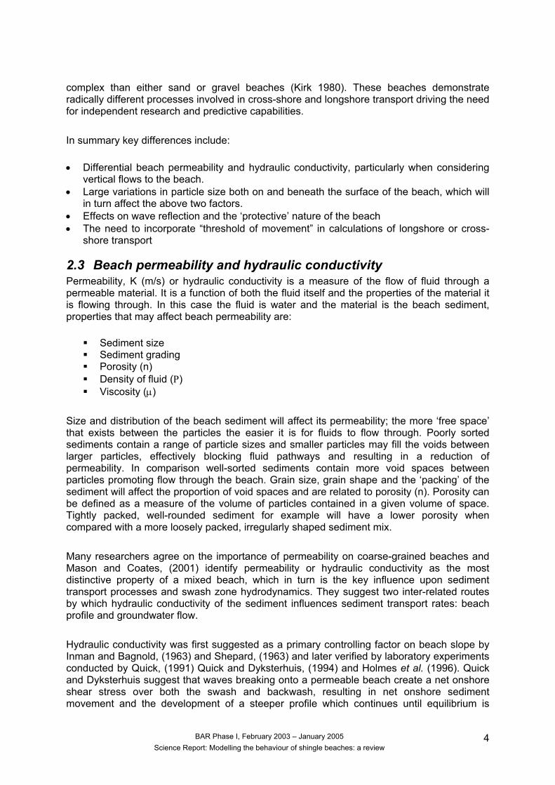
2.4 Swash zone dynamics Shingle beaches can support a steeper gradient than sand beaches and gradients in excess of 1/5 are common (Van Wellen et al. 2000). This steep gradient means that waves can travel much further inshore before breaking and that energy dissipation through breaking is concentrated over a much narrower zone. An important consequence of this energetic unsaturated breaker zone is that the swash zone can be of a similar width to the surf zone and accordingly sediment transport within the surf zone is of more importance than on sand beaches. Swash infiltration onto an unsaturated beach enhances onshore transport and profile steepening and is promoted by coarse-grained sediments. In contrast groundwater seepage on a saturated beach promotes offshore sediment transport and profile lowering (Figure 1). The importance of groundwater as a controlling factor on swash hydrodynamics, sediment transport and beach profile development is increasingly recognised although to date field and laboratory experiments have in the majority of cases concentrated on sandy beaches. For a detailed review of groundwater behaviour on sand beaches see Baird and Horn (1996) and Blanco (2003). The existence, importance and effects of a seepage face on mixed shingle beaches and the importance for swash zone sediment transport is uncertain. The higher infiltration capacity of gravel increases the potential for infiltration during the swash and is thought to be responsible for the formation of a berm at maximum run-up (Van Wellen et al. 2000). Yet the specific retention of shingle is low resulting in higher potential rates of exfiltration during backwash. The wide swash zone observed on shingle beaches (discussed above) means that infiltration/exfiltration processes on shingle mixed beaches is therefore more complex and a more important in beach development than on sand beaches.


5

Dry beach face

Exit point Seepage face

Wet beach face

Sea level

Groundwater flow direction

Figure 1. Definition sketch of a seepage face, general direction of flow within the beach is indicated. (Adapted from Masselink and Turner 1999)

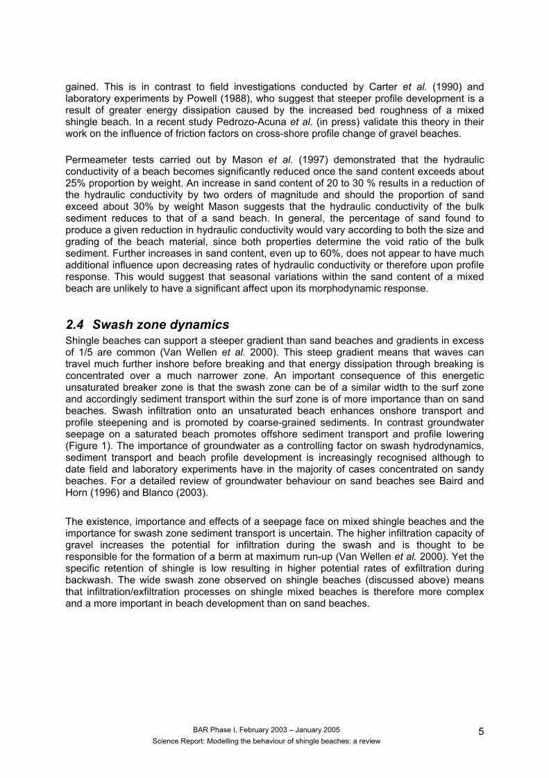
The existence, importance and effects of a seepage face on mixed shingle beaches and the importance for swash zone sediment transport is uncertain. The higher infiltration capacity of gravel increases the potential for infiltration during the swash and is thought to be responsible for the formation of a berm at maximum run-up (Van Wellen et al. 2000). Yet the specific retention of shingle is low resulting in higher potential rates of exfiltration during backwash. The wide swash zone observed on shingle beaches (discussed above) means that infiltration/exfiltration processes on shingle mixed beaches is therefore more complex and more important in beach development than on sand beaches. The situation is further complicated by the presence of non-Darcian flow through the mixed sediment. If a mixed sand and shingle layer exists at a depth below the surface at a level that is higher than the tide induced fluctuations of the water table, then percolation rates through overlying sediment will be significantly reduced. This is because the presence of the sand fraction affects both hydraulic conductivity and specific retention of the mixed sediment, with the net affect that sand shingle mixtures remain saturated for longer. This in turn will increase rates of material transport, as saturated sediment is more mobile. To date there are no field experiments that have measured differential infiltration during swash and backwash on a mixed shingle beach, mainly due to the inhospitable environment, which makes deployment of sensitive electronic instruments difficult and expensive. However 1:1 scale physical modelling tests were recently conducted by Blanco, (2003) in the GWK wave basin in Hanover Germany. The results of which are outlined below. A detailed study was conducted with the aim of applying and assessing current theories of gravel beach behaviour on both gravel and a mixed beach replica. Findings demonstrated that in fact mixed beaches show very different responses to gravel beaches when subjected to the same wave conditions. In particular swash and backwash processes were observed to be very different. Gravel beaches as expected demonstrated high levels of percolation as


6

water quickly infiltrated down through the beach material, reducing the effect of swash processes. Mixed beaches in comparison showed only small levels of percolation and this occurred much more slowly, the net effect being that a fringe of water exists on the beach face, which continues to run up the slope. Differences in levels of percolation were attributed to the elevated water table level, observed within the mixed beach structure. Mixed beach sediments appear to be a good storage medium for water and show a greater resistance to drainage (water enters the porous material far more easily than it leaves it). In addition Blanco demonstrated that the response of the water table to waves on a mixed shingle beach is far slower than on a gravel beach and the response is cumulative (the effect of new waves is added to the existing effects of previous waves). This ‘memory’ within the system results in an elevated water table and in general a more saturated beach, in theory promoting offshore transport during backwash and a profile lowering. This was supported by Blanco’s further work on profile development of mixed beaches. In general it was observed that mixed beach response is smaller and slower than the response for gravel beaches (40 –70% in terms of volume), taking longer to reach an equilibrium profile (3000 – 4500 waves as opposed to 2000 – 3000 waves). Beach crests are always of a lower elevation, as is step formation, which are in addition often irregular and difficult to locate. These factors combined make profile development for mixed shingle beaches more difficult to predict than was previously imagined Recent work conducted by Pedrozo-Acuna et al. (in press) at the University of Plymouth identified both bottom friction and transport efficiency (C-value) as a significant factor affecting shingle transport and swash zone profile development. Work involved successful combination of a higher order Boussinesq model with moving shoreline boundary (Lynett et al. 2002) coupled with a bedload transport model to investigate the key processes controlling profile development. It was discovered that by using dissimilar values for the sediment transport efficiency (C-value) in the uprush and backwash cycles, rather than a constant value, profile prediction could be improved. When C-values and bottom friction were kept the same in both the uprush and backwash cycles then accurate representation of profile evolution was impossible.

2.5 Wave Reflection As we have seen above shingle beaches are an extremely effective means of coastal defence and a large part of this defence is the ability to reflect up to 90% of all incident wave energy (Powell 1990). Although this is a significant feature of coarse-grained beaches, to date very few studies in the estimation of wave reflection for mixed beaches exist. The above sections have described the process by which oncoming waves may be dissipated through the beach; wave reflection describes how the remaining energy is reflected seaward. The coefficient of reflection can be written as:

KR = 1SSR

Where S1 is the incident wave energy and SR is the energy reflected. The coefficient of dissipation may also be defined as

KD = 1

1SSR−


7

Therefore the relationship between the two variables can be expressed as

KD = 21 RK−

However, when applied to mixed beaches it is necessary to consider the dissipative properties of the different sizes of beach material. There are two key aspects that will affect wave reflection on mixed beaches:

Beach slope Permeability

Mixed shingle beaches are less permeable than gravel beaches therefore less energy is absorbed into the beach making more energy available for reflection. However the profile lowering observed on mixed shingle beaches by Masselink and Turner (1999) will serve to reduce wave reflection of the beach. Davidson et al. (1994) observed that the slope of a mixed beach varied with the tidal cycle and that higher reflection coefficients were calculated for the steeper shore face gradients. He therefore concluded that tidal variation is an important factor in determining the reflection coefficient for mixed beaches. More recently Blanco, (2003) ran laboratory tests on simulated gravel and mixed beaches and calculated a larger coefficient value for gravel beaches compared with mixed beaches. She in contrast concluded that beach slope was the key factor in determining coefficient of reflection on a mixed shingle beach and that tidal variation had little effect.

2.6 Threshold of movement Threshold of movement refers to the critical or threshold fluid velocity above which individual grains become mobilised. The term is generally related to sediment size, which makes it difficult to describe for mixed shingle beaches as establishing critical thresholds of movement is complicated due to the particle interactions. The majority of work on initial motion of sediments is based upon the shields diagram (Shields 1936). Soulsby (1997) later adapted this work by plotting the shields parameter against a dimensionless grain size D*, making it available for practical application. Shields curve describes threshold of motion in terms of the ratio between the bed sheer stress acting to move the particle and the submerged weight of the grain that counteracts this. However, the shields parameter is not applicable to heterogeneous sediment (mixed beaches) being derived for strictly uniform sediments. Other researchers have attempted to model threshold of movement for mixed sediment situations but contradictions within the literature exist. Einstein, (1950) first pointed out that coarser grain sizes exposed at the surface protrude more into the flow and thus will feel a preferentially larger drag force, this work is further validated by Naden (1987). However, Komar and Li (1986) suggest that the smaller particles will be removed first, as they have a lower critical threshold. Egiazaroff (1965) conducted tests that considered both of these elements and concluded that the net effect was a small tendency for coarser grains to be harder to move than finer grains Blanco (2003), states that the grain size of a given fraction will have three different effects on the mobility of that fraction.

Absolute size effect: for a given grain shape and density, the mass and area of the grain exposed to the flow is given by the absolute size of the fraction. In a homogenous grain size fraction at a given bed shear stress, the mobility of the particles increase when grain size decreases, due to a reduction in the weight of the particles (the resisting force).


8

Hiding effects: The threshold of movement for any given size fraction depends on both the absolute size of the fraction itself and the size of the surrounding particles. In a bed consisting of many different size fractions the larger grains protrude more and the smaller grains may hide behind or in between them, therefore the larger grains are more easily moved than the smaller grains.

Relative protrusion to the flow (described above) It can be concluded that mass and area effects make coarser grains harder to move than finer grains whereas hiding effects make coarser grains easier to move than finer grains. A laboratory study conducted by Kuhnle (1994) used mixed sediment mixtures of 0, 10, 25, 45 and 100% gravel, although not particularly representative of actual mixed beaches, being derived fluvial systems, these are the most relevant to date. Kuhnle concluded that when using both homogenous mixtures (100% sand and 100% shingle) all sizes began to move at the same-recorded bed shear stress. However in bi modal mixtures, all the sand fractions began to move at nearly the same shear stress whereas the shingle fractions clearly demonstrated that threshold of movement was a function of grain size. Kuhnle concluded that differential entrainment patterns observed were due to the high percentage of sand within the mixtures. In mixtures containing 50% and above sand, interstices became filled but sufficient sand remained on the surface, available for entrainment. However, in mixtures with a lower percentage of sand, the sand became trapped within the interstices and was therefore not available for transport. Once the surface layer of sand is removed, coarser grains are exposed to the flow and become entrained. Field investigations of shingle thresholds of movement are scarce but in 1991, Walker et al. measured velocities of sand and shingle transport through an inlet, when a barrier in California was artificially breached for engineering purposes. They observed a threshold velocity of 1.6ms-1 for gravel sizes between 5 to 200mm, with no differential transport between sizes. Several other authors have observed this ‘equal entrainment mobility’ (Lu and Wu 1999, Wilcock 1997) but it should be noted this has only applied to equilibrium transport conditions which are rare in nature (Parker 1990). The causes and conditions that promote equal mobility are as yet not fully understood. .

3 Predicting and Modelling mixed shingle beaches The above section has outlined the present state of knowledge in terms of mixed shingle beach composition and influences upon sediment transport processes and profile development. The following section outlines modelling approaches, past and present, both in general and more specifically for mixed shingle beaches.

3.1 Existing predictive methods When discussing predictive techniques for any coastal area it is important to consider both the long-term and the short term ‘event’ based response of beaches, this can be achieved using either physical models or numerical models.

3.2 Physical models Physical models are laboratory based and are either conducted in a wave flume or a wave basin, either method can provide valuable information but the use of these models is limited due to costs and availability of both facilities and suitable modelling material. Mobile bed modelling at smaller scales can also be employed but is further limited by issues


9

of scale and adequate representation, as it is always necessary to draw some compromise between the requirements of the different processes that need to be simulated. When modelling any sand-gravel beach sediment, according to Powell (1990) there are three main requirements that need to be reproduced.

Beach permeability (and hence slope) Threshold of sediment movement Relative magnitude of onshore/offshore movement

An additional requirement for mixed beaches, noted by Blanco (2003) would be bedload/suspension load. Although there are four requirements to be met, model sediment particles have only two characteristics;

Size Specific gravity

It is therefore highly unlikely that all four requirements can be modelled simultaneously and some compromise is always necessary in the selection of model material. Additional complications arise due to the fact that the available material has only a limited range of specific gravities. Often the selection of model material is based as much upon availability as it is suitability for the tests in hand. Many commercial and research studies use crushed anthracite as the model material and this is deemed acceptable to scaling narrow graded gravel beds. However, small scale modelling of mixed shingle beaches is limited due to the incompatibility of the different size fractions within the same model material (Powell 1990).

3.2.1 Numerical models In recent years increasing reliance has been placed upon numerical models, due to their ability to link morphological changes to specified hydrodynamic conditions (Brampton and Southgate 2001). Numerical models can be broadly divided into parametric and physics based. Parametric models use observed results from laboratory or field studies while physics based models attempt to account explicitly for the key physical processes active across the foreshore (Blanco 2003). Numerical models can be further categorised by considering how they deal with coastal morphological change in space and throughout time, most models belong to only one type and as yet no model has been developed that can deal with variables of both time and space (Appendix 1). Present day modelling techniques have their strengths but none are able to accurately simulate all of the complex processes and interactions that affect mixed beach behaviour and response. To date most numerical models have been derived for sand beaches and extrapolated for use on coarser grained sediments. The main problems encountered in this method are set out in Coates and Mason (1998) and Blanco et al. (2000). Their conclusions are as follows Models assume a simplistic description of beach sediment; usually considering the entire

beach as being composed of only a single D50 value or other simple parameter. Models assume that beaches do not vary in composition, across shore, along shore or at

depth in situ or over time.


10

Flows within the beach are ignored (infiltration, exfiltration and interactions with groundwater)

Models assume a simple threshold of motion as defined by the singular particle size.

3.2.2 Longshore transport models Predictive techniques for modelling longshore transport processes on coarse-grained beaches have been derived using both numerical modelling techniques and applying known transport equations, such as the CERC formula. In many cases these were developed for sand beaches and were subsequently adapted and applied to shingle beaches, for example Van Wellen et al. (1999), described later in this section. However sediment transport processes are significantly different on sand beaches compared to those on shingle. Any transport model developed for sand beaches will concentrate primarily on the surf zone, in which spilling breakers dissipate energy and transport occurs through suspended load. On shingle beaches in contrast the majority of transport occurs as bedload and as we have already seen swash zone processes are more dominant than surf zone. In this respect it would seem that transport equations for coarse-grained sediments would be the most applicable for mixed shingle beaches. However, as the review produced by Van Wellen et al. (1999) demonstrates applicability is met with limited success. In total 12 existing formula were identified for testing and predictions derived from these formula were compared with measured annual transport rates from a shingle beach. Investigations confirmed that only a few equations have ever been developed specifically for longshore sediment transport on coarse-grained beaches and most of these involved calibration from a very limited dataset. In the majority of cases longshore transport rates were grossly over estimated. Energetics based equations were found to give reasonable results despite being derived for sand beaches, but the most accurate predictions were from formula previously validated for sites very similar to the one used. This research highlights the urgent need for the collection of good quality field data in order to better validate longshore transport models. Only through more rigorous testing can these equations ever be considered reliable and applied with any confidence. Cross-shore numerical models are also underdeveloped at present, mainly due to the uncertainty that surrounds the underlying hydrodynamics of shingle beaches and/or the inability to model the processes adequately. Hence to date no process-based model is available to predict the response of coarse grained or mixed beaches to given hydrodynamic forcing (Blanco 2003). Present research into providing such models is being undertaken at HR Wallingford, who are working on an extension of OTTP-1D (one dimensional swash zone model with a porous layer) towards a morphological capability (Clarke and Damgaard 2002). And at the University of Plymouth, where work is being conducted into combining a 1-D phase resolving numerical wave model (based upon Boussinesq equations) with a morphodynamic module (Lawrence et al., 2003).

4 Existing models for mixed shingle beaches

4.1 Litpack: An integrated modelling system LITPACK is a professional engineering software package designed to model non-cohesive sediment transport in waves and currents, littoral drift processes, coastline evolution and profile development of beaches.


11

The basic structure of the software consists of a variety of modules, all of which have a deterministic approach and each of which focus upon a different aspect of coastal evolution and prediction. This allows for the consideration of many variables and allows determination of the dominating processes in action. For example the simulation of a multi barred profile which contains a variety of grain sizes is subject to errors when taking a traditional energy flux approach. With LITPACK these sorts of variables can be taken into account and the software provides a valuable tool for engineering, management and planning applications in the coastal zone.

4.1.1 Modelling applications The Sediment Transport Program (STP) lies at the core of the LITPACK modelling system and is integrated in all LITPACK modules to form the basic element for all sediment transport calculations. Applications related to LITPACK and research questions that can be investigated include: Sediment budgets along coasts Impact assessment for coastal works Optimisation of beach restoration Optimisation of coastal protection Design and optimisation of beach nourishment Channel backfilling

The primary feature of the LITPACK modelling system is the integrated modular structure, the main modules included are outlined below: Non-cohesive sediment transport (LITSTP) Longshore current and littoral drift (LITDRIFT) Coastal evolution (LITLINE) Cross-shore profile evolution (LITPROF) which is of particular importance when

considering this study Sedimentation in trenches (LITTREN)

For the purposes of this study the longshore current and littoral drift module (LITDRIFT) and the cross-shore profile evolution module (LITPROF) will be examined and described in more detail.

4.1.2 LITDRIFT – longshore current and littoral drift The LITDRIFT module combines the non-cohesive sediment transport module with a coastal hydrodynamic module to give a deterministic description of the littoral drift. LITDRIFT simulates the cross-shore distribution of wave height, setup and longshore current for an arbitrary coastal profile and provides a detailed deterministic description of the cross-shore distribution of longshore sediment transport for both regular and irregular sea states. The longshore and cross-shore momentum balance equation is solved to give the cross-shore distribution of longshore current and setup. LITDRIFT calculates the net/gross littoral drift over a specified period and important factors such as linking water levels to and the profile to the incident sea state are recognised and included.


12

4.2 Cross shore profile development LITPROF describes cross-shore profile changes by solving the bottom sediment continuity equation, based upon the sediment transport rates calculated by STP. LITPROF takes into account the effects of changing morphology on the wave climate and transport regime enabling a simulation of profile development for a time varying incident wave field. LITPROF also has the capability of including structures and impermeable bottom layers to the profile, modelling areas that can not be eroded.

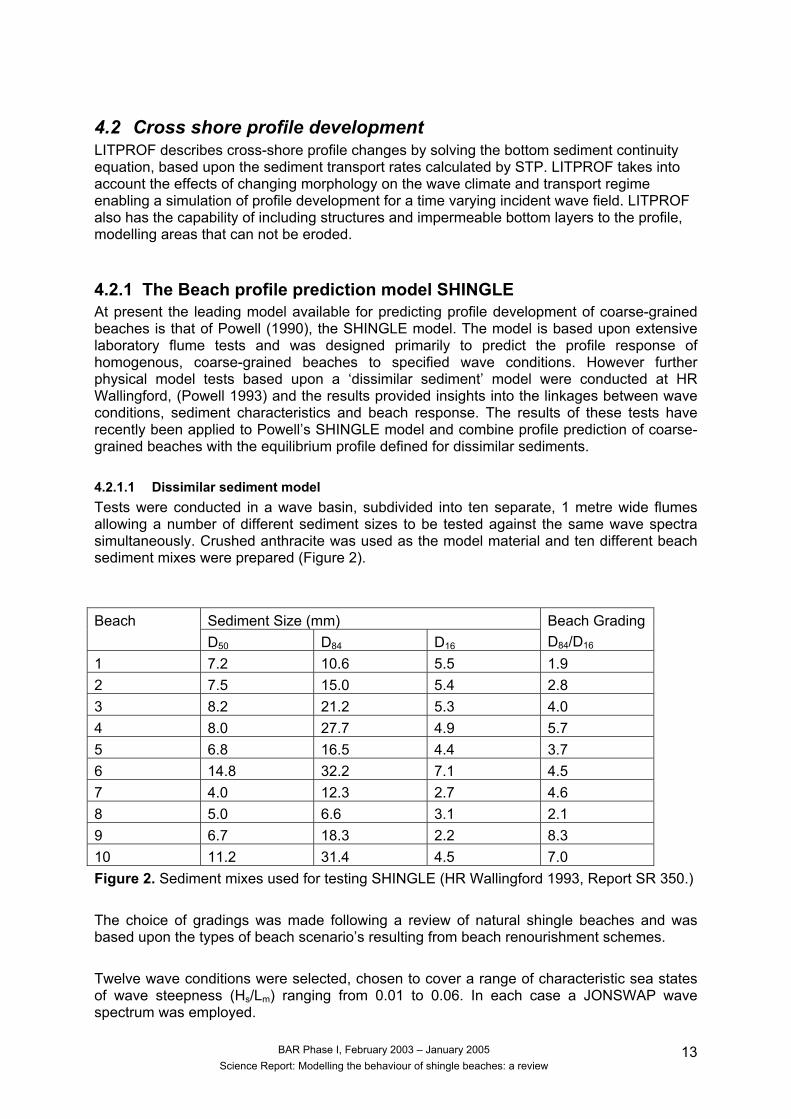
4.2.1 The Beach profile prediction model SHINGLE At present the leading model available for predicting profile development of coarse-grained beaches is that of Powell (1990), the SHINGLE model. The model is based upon extensive laboratory flume tests and was designed primarily to predict the profile response of homogenous, coarse-grained beaches to specified wave conditions. However further physical model tests based upon a ‘dissimilar sediment’ model were conducted at HR Wallingford, (Powell 1993) and the results provided insights into the linkages between wave conditions, sediment characteristics and beach response. The results of these tests have recently been applied to Powell’s SHINGLE model and combine profile prediction of coarse-grained beaches with the equilibrium profile defined for dissimilar sediments. 4.2.1.1 Dissimilar sediment model Tests were conducted in a wave basin, subdivided into ten separate, 1 metre wide flumes allowing a number of different sediment sizes to be tested against the same wave spectra simultaneously. Crushed anthracite was used as the model material and ten different beach sediment mixes were prepared (Figure 2).

Sediment Size (mm) Beach D50 D84 D16

Beach Grading D84/D16

1 7.2 10.6 5.5 1.9 2 7.5 15.0 5.4 2.8 3 8.2 21.2 5.3 4.0 4 8.0 27.7 4.9 5.7 5 6.8 16.5 4.4 3.7 6 14.8 32.2 7.1 4.5 7 4.0 12.3 2.7 4.6 8 5.0 6.6 3.1 2.1 9 6.7 18.3 2.2 8.3 10 11.2 31.4 4.5 7.0 Figure 2. Sediment mixes used for testing SHINGLE (HR Wallingford 1993, Report SR 350.) The choice of gradings was made following a review of natural shingle beaches and was based upon the types of beach scenario’s resulting from beach renourishment schemes. Twelve wave conditions were selected, chosen to cover a range of characteristic sea states of wave steepness (Hs/Lm) ranging from 0.01 to 0.06. In each case a JONSWAP wave spectrum was employed.


13

Data from the model was collected in two basic formats:

Computer generated profiles Sediment size distributions for pre-defined locations on the beach profile

Trends in test results are outlined below: Profile response of beaches demonstrated that under storm conditions a wider beach grading experiences a higher degree of erosion than a more naturally graded beach. In addition these beaches are less likely to accrete under constructive swell conditions than a more narrowly grading beach. It is agreed that wave action sorts/reworks beach sediments and that in general this results in a movement of finer material down to the core of the beach leaving a coarser ‘armouring’ layer at the beach surface. This coarser surface layer also experiences cross-shore sorting which results in a variable distribution of coarse material across the surface of the beach profile. Although erosion occurred over the entire beach profile, the size classes of sediment moving offshore was determined by location on the profile. At the beach crest finer fractions of the surface layer were moved offshore while closer to the shoreline there was an offshore migration of the entire surface layer, this exposed the underlying sediment resulting in a surface layer similar in composition to the background beach material. Test results indicate that distinctly different surface sediment distributions exist for erosive and accretionary beach profiles. Erosion profiles showed the coarser material occurring in the wave breaker zone and to a lesser extent at the beach crest with the finer material being located at the shoreline. On accretionary profiles in comparison, there was a steady increase in mean sediment size from the beach toe to the beach crest. Based upon these results an equation for the ‘equilibrium slope’ of mixed shingle sediments was derived (3-1), incorporating influences of median sediment size, sediment grading and incident wave climate. Sin θ = 0.206 [(Hs/Lm) -0.220 (D84/D16) -0.394 (Hs/D50) -0.306] -0.567

(3-1) Where: sin = equilibrium slope

θ = Angle between slope and a horizontal line Hs = Wave height Hs/Lm = Wave steepness

Although these tests provide a basic outline of the behaviour of dissimilar sediments on a beach under laboratory conditions, to date there has been no field work undertaken on mixed shingle beaches to observe the cross-shore sorting and onshore/offshore movement of the different size classes of beach material. This information is of vital importance if a detailed understanding of mixed shingle beach behaviour in an actual coastal setting is ever to be produced. SHINGLE is an example of a parametric equilibrium cross-shore model (Appendix 1), developed by Powel of HR Wallingford in 1990 as a coastal management tool. Parametric modelling is at present the most suitable tool for describing shingle beaches, as the surface of a shingle beach, by exhibiting a number of readily identifiable features is particularly


14

amenable to a parametric description. In addition the parametric model requires little or no understanding of the underlying hydrodynamics, an area of considerable uncertainty with regard to shingle beaches. Consequently parametric modelling was adopted for SHINGLE. SHINGLE is used both commercially and for research purposes and remains the leading model available for predicting profile development on shingle beaches. The model allows the user to predict changes to shingle beach profiles based upon prescribed input conditions of sea state, water level, existing profile, sediment size and underlying stratum. Profile shape and position against an initial datum can be predicted and the confidence limits for the predictions can be determined. This capability allows SHINGLE to be used for predicting the potential erosion of existing shingle beaches or to predict the performance of shingle renourishment schemes.

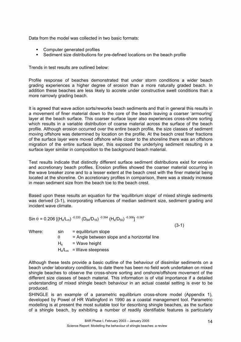
4.2.2 Model test The model tests to develop SHINGLE were conducted in a random wave flume, measuring 42 metres in length, 1.5 metres in width and with a depth of 1.4 metres. The operating water depth was within the range of 0.7 to 0.9 metres. Prior to running the tests a brief study was undertaken to determine the range of typical shingle sizes and gradings for UK beaches (Figure 3). Based upon these results four combinations of shingle size and grading were selected for reproduction in the model tests (Figure 4).

Site D10 D50 D100 Grading D85/D15 Seaford 6.1 13.7 38.0 2.73 Whitstable 7.6 12.6 50.0 2.41 Chesil (Portland) 23.8 30.0 - - Chesil (W. Bexington) 8.5 10.0 13.0 1.34 Littlehampton 7.3 13.0 42.0 2.33 Hayling Island 7.0 16.0 64.0 4.00

Figure 3. Typical shingle sizes of the UK (HR Wallingford, Report SR 219)

MIX D10 D50 D90 Grading D85/D151 6.9 10.0 22.9 2.6 2 7.3 10.4 19.1 2.2 3 17.3 30.0 46.1 2.2 4 11.6 24.0 38.7 2.6

Figure 4. Sediment mixes derived (HR Wallingford, Report SR 219) Before running the laboratory tests a model scale should be derived, due to the magnitude of the desired wave conditions combined with the limitations of the test facility, a nominal model scale of 1.17 was chosen. At this scale it was determined that a mix of crushed anthracite would provide the best representation of a natural shingle beach material in terms of permeability, sediment mobility, threshold and onshore offshore transport characteristics. In total 131 detailed tests were conducted against 29 different wave spectra, (all tests employed waves of the Jonswap spectral type) using the 4 different material sizes and gradings already outlined. Each test was run for 3000 waves, at which point it was assumed


15

the beach profile had achieved a near-stable state. Testing was based on various wave steepness groupings, beginning with the least severe waves in each grouping, building up to the most severe conditions. Three sets of measurements were taken during each test, beach profile, wave run up exceedence distribution and wave energy dissipation coefficients, profile measurements were taken at 500 wave intervals. Upon completion of a set of tests the ‘beach’ was remoulded to its initial profile and the sequence was started again for waves of the next steepness grouping.

4.2.3 Building the model Following analysis of the laboratory data, it was possible to identify key variables that influence shingle beach profile development:

Wave height (Hs) Wave period (Tm) Wave duration (N) Beach material size (D50) Beach material grading (D85/D15) Effective thickness of beach material (DB) Foreshore level (Dw) Still Water level (SWL) Initial beach profile Wave spectrum shape Angle of wave attack

Of these factors the first 6 were determined from the flume tests, the remaining factors were observed during previous research. Using this information shingle was constructed, designed to address two aspects of profile prediction:

1. Predicted profile shape 2. Location of the predicted profile against an initial datum.

The predicted beach profile is broken into three curves between distinct limits;

1. Beach crest and SWL 2. SWL and the top edge of the profile step 3. The top edge of the profile step and the lower limit of profile deformation

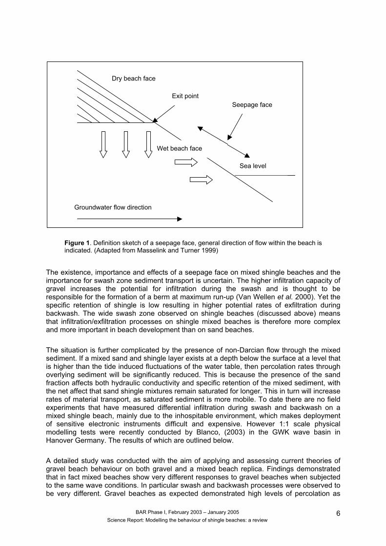
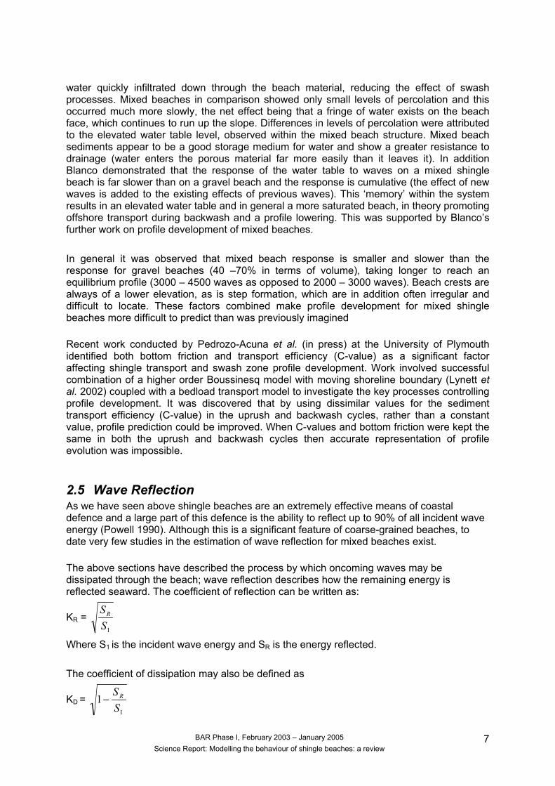
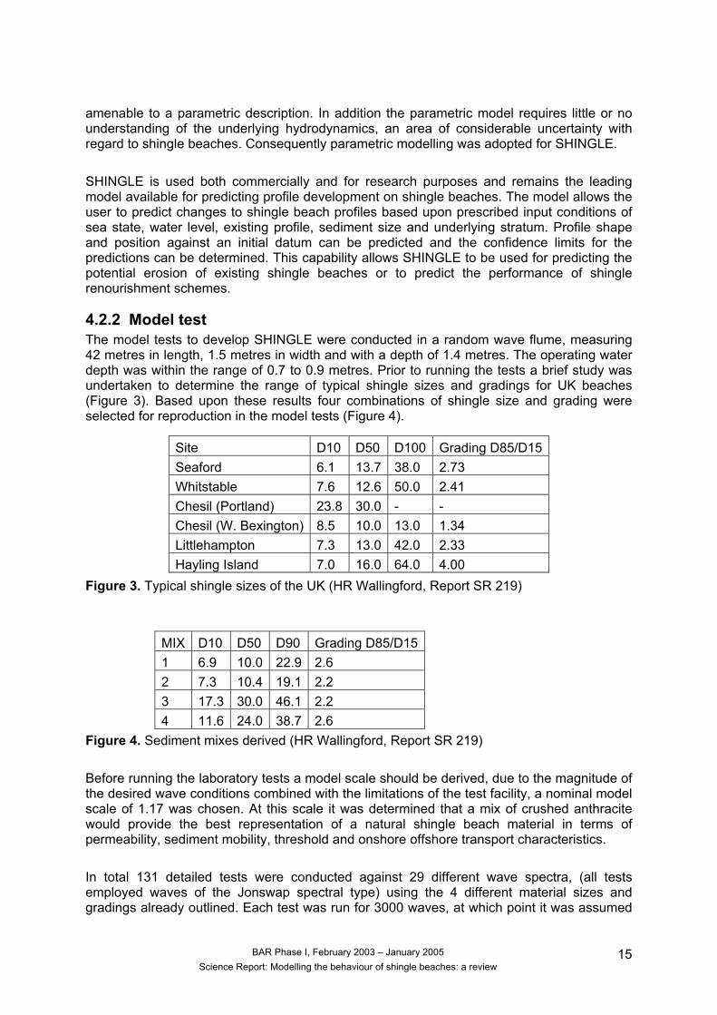
In effect the model feeds new beach profile chainage and elevation data into a system and uses specified input parameters to calculate a new profile chainage position and elevation, based upon a series of equations underlined by the area calculation. The position of the predicted profile relative to the initial profile assumes that the beach material moves only in an onshore-offshore direction and that longshore transport rates are in effect zero. The areas under the two curves are compared against a common datum and the predicted profile is shifted along the SWL axis until the areas equate to provide the location for the predicted profile. The crux of the model lies in calculating the new beach elevations for each chainage point working from a series of logical expressions. New elevations are calculated for every chainage position at 0.10m increments. The model then calculates the area of beach within each increment (Figure 5). A series of checks are run, to ensure that:

Final areas are based upon beach area only (beach stratum area is removed)


16

Final volumes are always positive values Any error values produced during the process are taken into account and area in m2

is either added or removed from the incremental areas. The final beach area is derived from cumulative beach areas starting at 0 chainage and extending seawards at increments of 0.10m for the length of the profile. Figures 5 and 6 demonstrate how the model works.

Figure 5: Incremental beach area calculations

4.2.4 Model operation There are three main elements to the model, inputs, profile prediction and outputs; the input data required are;

Initial beach profile including measurements of the foreshore Beach particle size (D50 ) Offshore wave height (Hs) Offshore wave period (Tm) Still water level (SWL) Depth and slope of the underlying non mobile stratum Effective beach thickness ration (DB/D50)

Of these the user inputs field data collected for the first 4 points, the final two are calculated within the model automatically. If input values fall outside the working limits of the model then an error message is displayed to warn the user. In addition if input wave and foreshore conditions indicate a depth limited wave then breaking wave equations are employed to modify the offshore wave values to give appropriate values at the beach.


17

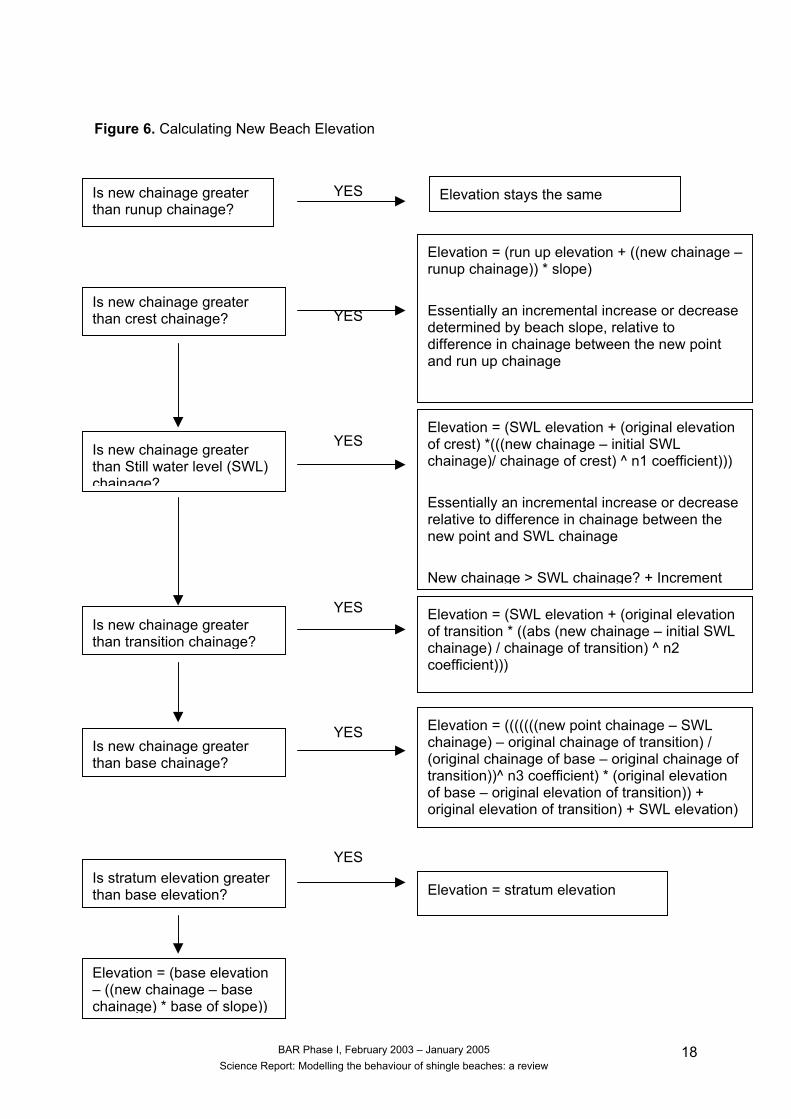
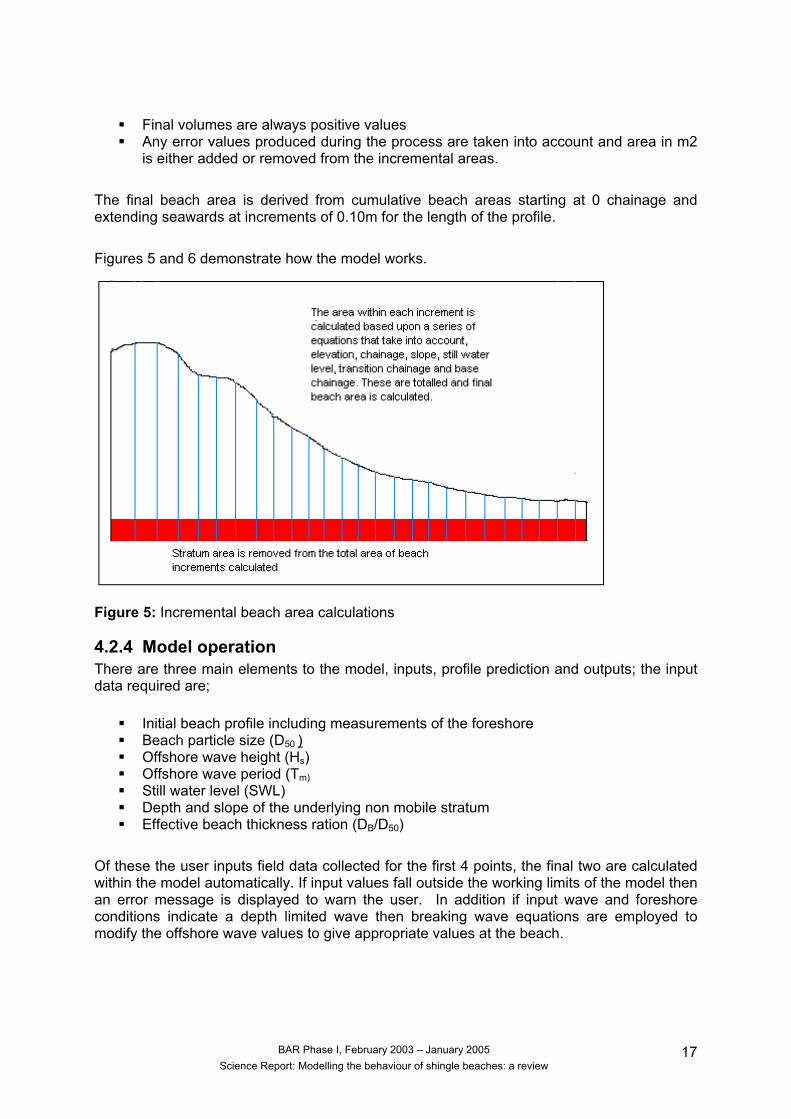
Figure 6. Calculating New Beach Elevation

Elevation stays the same YES

Is new chainage greater than runup chainage?

YES

YES

YES

YES

YES

Is new chainage greater than crest chainage?

BAR Phase I, February 2003 –Science Report: Modelling the behaviour of

Elevation = (run up elevation + ((new chainage –runup chainage)) * slope) Essentially an incremental increase or decrease determined by beach slope, relative to difference in chainage between the new point and run up chainage

Is new chainage greater than Still water level (SWL) chainage?

Elevation = (SWL elevation + (original elevation of crest) *(((new chainage – initial SWL chainage)/ chainage of crest) ^ n1 coefficient))) Essentially an incremental increase or decrease relative to difference in chainage between the new point and SWL chainage New chainage > SWL chainage? + Increment

Is new chainage greater than transition chainage?

Elevation = (SWL elevation + (original elevation of transition * ((abs (new chainage – initial SWL chainage) / chainage of transition) ^ n2 coefficient)))

Elevation = (((((((new point chainage – SWL chainage) – original chainage of transition) / (original chainage of base – original chainage of

Is new chainage greater than base chainage?

transition))^ n3 coefficient) * (original elevation of base – original elevation of transition)) + original elevation of transition) + SWL elevation)

YES Is stratum elevation greater than base elevation?
Elevation = stratum elevation
Elevation = (base elevation – ((new chainage – base chainage) * base of slope))

January 2005 shingle beaches: a review

18

5 References Baird, A.J. and Horn, D.P. 1996. Monitoring and modelling groundwater behaviour in sandy beaches. Journal of coastal research, 12, 630-640 Brunn, P. Coast erosion and the development of beach profiles. US Army Corps of Engineers, BEB, TM – 44, 1954. Brampton, A.H. and Southgate, H.N. 2001. Coastal morphology modelling: A guide to model selection and usage. Report SR 570. Carter, R.W.G. Orford, J.D. Forbes, D.L. and Taylor R.B. 1990. Morpho-sedimentary development of drumlin-flank barriers with rapidly rising sea level, Story Head, Novia Scotia. Sedimentary geology, 69, 117-138 Clarke, S. and Damgaard, J.S. 2002. Applications of a numerical model of swash flow on gravel beaches. Proceedings of the 28th international conference on coastal engineering. Cardiff, UK. Coates, T.T. and Mason, T. 1998. Development of predictive tools and design guidance for mixed beaches. Scoping study. HR Wallingford report TR 56. Davidson, M.A. Bird, P.A.G. Bullock, G.N. and Huntley, D.A. 1994. Wave reflection: field measurements, analysis and theoretical developments. Coastal dynamics 1994, (ASCE) 642-655. Dean, R.G. Equilibrium beach profiles: US Atlantic and Gulf coasts. University of Delaware, Department of Civil Engineering, Ocean Engineering, Report 12, 1977. Egiazaroff, I.V. 1965. Calculation of nonuniform sediment concentrations, journal of hydraulic engineering, 91, (4), 225-247. Einstein, H.A. 1950. The bed-load function for sediment transportation in open channel flows, Technical bulletin 1026, U.S. Department of the army, soil conservation service. Fox, W.T. Modelling coastal environments. In R.A. Davis, Jr (Editor), Coastal Sedimentary Environments. Second Edition. Springer-Verlag, New York, 665-705. Holmes, P. Baldock, T.E. Chan, T.C. and Neshaei, M.A.L. 1996. Beach evolution under random waves. Proceedings of the 25th international conference on coastal engineering (American society of civil engineers), 3006-3019. Hughes, S.A. and Chiu, T.S. The variations in beach profiles when approximated by a theoretical curve, University of Florida, Coastal and Oceanographic Engineering Department, Report TR/043, 1981


19

Inman, D. L. and Bagnold, R.A. 1963. Littoral processes. In: The sea, (Ed.) M. N. Hill. NY Interscience. Keulegan, G.H. Krumbien, W.C. Stable configuration of the bottom slope in shallow water and it’s bearing on geological processes. Trans Amer Geophys Union, 30, No 6, 1949 Kirk, R.M. 1980. Mixed sand and gravel beaches: Morphology, processes and sediments. Progress in physical geography. 4, 189 – 210. Komar, P.D. and Li, Z. 1986. Pivoting analyses of the selective entrainment of sediments by shape and size with application to gravel threshold. Sedimentology, 33, 425-436. Kuhnle, R.A. 1994. Incipient motion of sand-gravel sediment mixtures. Journal of hydraulic engineering, (119) 1400-1415. Lakhan, V.C. 1986. Modelling and simulating the morphological variability of the coastal system. Presented at the International congress on applied systems research and cybernetics. August 18, 1986, Baden-Baden, Germany. Lawrence, J. Chadwick, A.J. and Flemming, C. 2000. A phase-resolving model of sediment transport on coarse-grained beaches. 27th International conference on coastal engineering. (ASCE), Sidney, Australia, 624 – 636. Lopez de san Roman-Blanco, B. Coates, TT. Peet, A.H. and Damgaard, J.S. 2000. Development of predictive tools and design guidance for mixed sediment beaches. HR Wallingford Report TR 102. Lopez de San Roman-Blanco, B. 2001. Morphodynamics of mixed beaches, unpublished transfer Mphil/Ph.D. Report. Civil and environmental engineering department, Imperial College, London. Lopez de San Roman-Blanco, B. Coates, T.T. and Whitehouse R.J.S. 2003. Development of predictive tools and design: Guidance for mixed beaches. Stage 2 Final report. Report SR 628 HR, Wallingford. Lu, J.Y and Wu, I.W. 1999. Movement of graded sediment with different size ranges. International journal of sediment research. 14 (3) 9 – 22. Lynett, P.J. Wu, T.R. and Liu, L.F.P. 2002. Modelling wave runup with depth-integrated equations. Coastal engineering, 46, 89-107. Mason, T. Voulgaris, G. Simmonds, D.J. and Collins, M.B. 1997. Hydrodynamics and sediment transport on composite (mixed sand and shingle beaches): a comparison. Coastal dynamics 1997 (American society of civil engineers), 48-57. Mason, T and Coates, T.T. 2001. Sediment transport processes on mixed shingle beaches: A review for shoreline management. Journal of coastal research, (17) 3, 645-657.


20

Masselink, G and Turner, I. 1999. The effect of tides on beach morphodynamics. In Short, A. (ED) Handbook of beach and shoreface morphodynamics. John Wiley and sons, Ltd. Sydney. Naden, P. 1987. An erosion criterion for gravel bed-rivers. Earth surface processes and landforms, 12, 83-93 Parker, G. 1990. Surface-based, bedload transport relation for gravel rivers. Journal of hydraulic research. 28 (4) 417435 – 41. Pedrozo-Acuna, A. Simmonds, A.J. Otta, A.K. and Chadwick, A.J. (In press) On the cross-shore profile change of gravel beaches, school of engineering, University of Plymouth. Powell, K.A. 1986. The hydraulic behaviour of shingle beaches under regular waves of normal incidence. PhD Thesis, University of Southampton. Powell, K.A. 1988. The dynamic response of shingle beaches to random waves. Proceedings of the 21st international conference on coastal engineering (American society of civil engineers), 1763-1773. Powell, K.A. 1990. Predicting short term profile response for shingle beaches. HR Wallingford Report SR 219 UK. Powell, K.A. 1993. Dissimilar sediments: Model tests of replenished beaches using widely graded sediments. HR Wallingford report SR 350, UK. Pye, K. 2001. The nature and geomorphology of coastal shingle. In: Ecology & Geomorphology of Coastal Shingle, eds.Packham, J.R., Randall, R.E., Barnes, R.S.K. & Neal, A.Westbury Academic and Scientific Publishing, 2-22. Quick, M.C. 1991. Onshore-offshore sediment transport on beaches. Coastal engineering, 15, 313-332. Quick, M.C. and Dyksterhuis, P. 1994 Cross-shore transport for beaches of mixed sand and gravel. International symposium: Waves-physical and numerical modelling (Canadian society of civil engineers), 1443-1452. Rivet, P. 1972. Introduction to simulation. McGraw-Hill, New York. Shepard, F. P. 1963. Submarine geology. New York. Harper and Row. Shields, I.A. 1936. Anwendung der ahnlichkeitmechanik under der turbulenzforschung auf die gescheibebewegung, Mitt. Preuss Ver. Anst. 26, Berlin, Germany. Soulsby, R.L. 1997. Dynamics of marine sands: A manual for practical applications. HR Wallingford report SR 466.


21

Van der Meer, J.W. Rock slopes and gravel beaches under wave attack. Delft Hydraulics, comm. No 396, 1988. Van Wellen, E. Chadwick, A.J. and Mason, T. 2000. A review and assessment of longshore sediment transport equations for coarse-grained beaches. Coastal engineering, 40, 243-275. Vellinga, P. A tentative description of a universal erosion profile for sandy beaches and rock beaches. Coastal Engineering 8, 1984 Walker, J.R. Everets, C.H. Schmelig, S. and Demirel, V. 1991. Observations of a tidal inlet on a shingle beach. Proceedings of coastal sediments 1991. American society of civil engineers, 975 – 989. Wilcock, P.R. 1997. The components of fractional transport rate. Water resources research. 33 (1) 247-258.


22

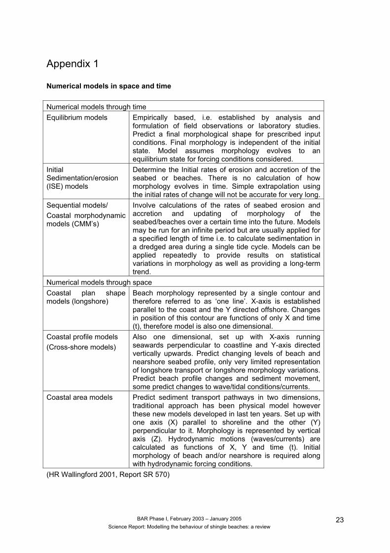
Appendix 1 Numerical models in space and time Numerical models through time Equilibrium models Empirically based, i.e. established by analysis and

formulation of field observations or laboratory studies. Predict a final morphological shape for prescribed input conditions. Final morphology is independent of the initial state. Model assumes morphology evolves to an equilibrium state for forcing conditions considered.

Initial Sedimentation/erosion (ISE) models

Determine the Initial rates of erosion and accretion of the seabed or beaches. There is no calculation of how morphology evolves in time. Simple extrapolation using the initial rates of change will not be accurate for very long.

Sequential models/ Coastal morphodynamic models (CMM’s)

Involve calculations of the rates of seabed erosion and accretion and updating of morphology of the seabed/beaches over a certain time into the future. Models may be run for an infinite period but are usually applied for a specified length of time i.e. to calculate sedimentation in a dredged area during a single tide cycle. Models can be applied repeatedly to provide results on statistical variations in morphology as well as providing a long-term trend.

Numerical models through space Coastal plan shape models (longshore)

Beach morphology represented by a single contour and therefore referred to as ‘one line’. X-axis is established parallel to the coast and the Y directed offshore. Changes in position of this contour are functions of only X and time (t), therefore model is also one dimensional.

Coastal profile models (Cross-shore models)

Also one dimensional, set up with X-axis running seawards perpendicular to coastline and Y-axis directed vertically upwards. Predict changing levels of beach and nearshore seabed profile, only very limited representation of longshore transport or longshore morphology variations. Predict beach profile changes and sediment movement, some predict changes to wave/tidal conditions/currents.

Coastal area models Predict sediment transport pathways in two dimensions, traditional approach has been physical model however these new models developed in last ten years. Set up with one axis (X) parallel to shoreline and the other (Y) perpendicular to it. Morphology is represented by vertical axis (Z). Hydrodynamic motions (waves/currents) are calculated as functions of X, Y and time (t). Initial morphology of beach and/or nearshore is required along with hydrodynamic forcing conditions.

(HR Wallingford 2001, Report SR 570)


23

Documents

MODELLING THE BEHAVIOUR OF SHINGLE BEACHES: A REVIEW › geography › researchprojects › BAR... · beaches is highly varied, some consisting almost entirely of shingle whilst others