Embed Size (px)
Citation preview
Modelling vortex-vortex and vortex-boundaryinteraction
Rhodri Burnett Nelson
DEPARTMENT OF MATHEMATICS
UNIVERSITY COLLEGE LONDON
A THESIS SUBMITTED FOR THE DEGREE OF
DOCTOR OF PHILOSOPHY
SUPERVISOR
Prof. N. R. McDonald
September 2009
I, Rhodri Burnett Nelson, confirm that the work presented in this thesis is my
own. Where information has been derived from other sources, I confirm that this has
been indicated in the thesis.
SIGNED
Abstract
The motion of two-dimensional inviscid, incompressible fluid with regions of constant vorticity
is studied for three classes of geophysically motivated problem. First, equilibria consisting of point
vortices located near a vorticity interface generated by a shear flow are found analytically in the
linear (small-amplitude) limit and then numerically for the fully nonlinear problem. The equilibria
considered are mainly periodic in nature and it is found that an array of equilibrium shapes exist.
Numerical equilibria agree well with those predicted by linear theory when the amplitude of the
waves at the interface is small.
The next problem considered is the time-dependent interaction of a point vortex with a single
vorticity jump separating regions of opposite signed vorticity on the surface of a sphere. Initially,
small amplitude interfacial waves are generated where linear theory is applicable. It is found that a
point vortex in a region of same signed vorticity initially moves away from the interface and a point
vortex in a region of opposite signed vortex moves towards it. Configurations with weak vortices
sufficiently far from the interface then undergo meridional oscillation whilst precessing about the
sphere. A vortex at a pole in a region of same sign vorticity is a stable equilibrium whereas in
a region of opposite-signed vorticity it is an unstable equilibrium. Numerical computations using
contour dynamics confirm these results and nonlinear cases are examined.
Finally, techniques based on conformal mapping and the numerical method of contour dynamics
are presented for computing the motion of a finite area patch of constant vorticity on a sphere and
on the surface of a cylinder in the presence of impenetrable boundaries. Several examples of impen-
etrable boundaries are considered including a spherical cap, longitudinal wedge, half-longitudinal
wedge, and a thin barrier with one and two gaps in the case of the sphere, and a thin island and
‘picket’ fence in the case of the cylinder. Finite area patch motion is compared to exact point vortex
trajectories and good agreement is found between the point vortex trajectories and the centroid
motion of finite area patches when the patch remains close to circular. More exotic motion of the
finite area patches on the sphere, particularly in the thin barrier case, is then examined. In the case
when background flow owing to a dipole located on the barrier is present, the vortex path is pushed
close to one of the barrier edges, leading to vortex shedding and possible splitting and, in certain
cases, to a quasi-steady trapped vortex. A family of vortex equilibria bounded between the gap in
the thin barrier on a sphere is also computed.
Acknowledgements
I would first and foremost like to express my heartfelt gratitude to my supervisor,
Robb McDonald, for all the help and guidance he has given me throughout my time
at UCL. It has been a pleasure to work with him and learn from his expertise, and I
thank him for playing a big part in making my time at UCL so enjoyable.
I would like to thank the Geophysical Fluid Dynamics group for the insightful
conversations and their input and in particular my predecessor, Alan Hinds, for all
his help and suggestions when I began my PhD. I am indebted to the UCL graduate
school for their financial assistance that has allowed me to attend some prestigious
conferences during my studies and of course, I owe a great deal of gratitude to my
funding body, the Natural Environment Research Council. I would also like to thank
my fellow PhD students who have created such a pleasant environment at UCL, and in
particular the students with whom I began my PhD, Tommy, Jo, Brian and Isidoros.
I owe a big thank you to all of the administrative staff who have been so helpful
throughout my PhD.
I also wish to warmly acknowledge the support of all of my friends and I would like
to thank Guy and Phil for the great holidays during my PhD and Will and Francois
for all of the entertainment in and around London.
I have a giant thank you to say to my girlfriend, Chierh, for her patience, kindness
and warmth (and for all the great meals that have kept me fit and healthy over the
past couple of weeks).
Yn olaf, hoffwn diolch fy teulu; fy Mam, Dad, Brawd, Chwaer ac fy Nain diffod-
diedig, am eu cariad a cymorth trwy gydol fy addysg. Hoffwn diolch fy Mam am eu
geiriau o cymorth yn y misoedd diweddar.
Contents
1 Introduction 1
2 Point vortex equilibria near a vortical interface: linear theory 7
2.1 An anti-symmetric translating equilibrium . . . . . . . . . . . . . . . 142.2 An infinite array of periodic vortices . . . . . . . . . . . . . . . . . . 23
2.2.1 Vortices in the irrotational flow region . . . . . . . . . . . . . 242.2.2 Vortices in the rotational flow region . . . . . . . . . . . . . . 43
2.3 Vortex street in a shear flow . . . . . . . . . . . . . . . . . . . . . . . 482.4 Summary . . . . . . . . . . . . . . . . . . . . . . . . . . . . . . . . . 56
3 Computation of non-linear equilibria on a vortical interface 61
3.1 Periodic symmetric equilibria . . . . . . . . . . . . . . . . . . . . . . 623.1.1 Point vortex in the irrotational flow region . . . . . . . . . . . 673.1.2 Point vortex in the rotational flow region . . . . . . . . . . . . 75
3.2 Periodic anti-symmetric equilibria . . . . . . . . . . . . . . . . . . . . 783.3 Planar anti-symmetric equilibrium . . . . . . . . . . . . . . . . . . . . 873.4 Summary . . . . . . . . . . . . . . . . . . . . . . . . . . . . . . . . . 90
4 Vortex-wave interaction on the surface of a sphere 92
4.1 Problem formulation and linear solution . . . . . . . . . . . . . . . . 954.2 Short time behaviour and the n = 1 system . . . . . . . . . . . . . . 1054.3 Truncating at n > 1 . . . . . . . . . . . . . . . . . . . . . . . . . . . . 1104.4 A non-linear stability calculation . . . . . . . . . . . . . . . . . . . . 1124.5 Non-linear computations . . . . . . . . . . . . . . . . . . . . . . . . . 1174.6 Summary and applications to planetary vortices . . . . . . . . . . . . 122
5 Finite area vortex motion on a sphere with impenetrable boundaries126
5.1 Contour dynamics in singly connected domains on a sphere . . . . . . 1325.2 Examples . . . . . . . . . . . . . . . . . . . . . . . . . . . . . . . . . 137
5.2.1 Ellipse in the stereographic plane . . . . . . . . . . . . . . . . 1375.2.2 Thin barriers with background flows . . . . . . . . . . . . . . 141
i
Contents ii
5.2.3 Longitudinal wedge . . . . . . . . . . . . . . . . . . . . . . . . 1475.2.4 Half-longitudinal wedge . . . . . . . . . . . . . . . . . . . . . 151
5.3 A doubly connected domain: Barrier with two gaps . . . . . . . . . . 1525.3.1 Background flows . . . . . . . . . . . . . . . . . . . . . . . . . 1605.3.2 Point vortex trajectories . . . . . . . . . . . . . . . . . . . . . 1625.3.3 Vortex patch motion . . . . . . . . . . . . . . . . . . . . . . . 165
5.4 Vortex Equilibria in a gap . . . . . . . . . . . . . . . . . . . . . . . . 1675.5 Conclusion . . . . . . . . . . . . . . . . . . . . . . . . . . . . . . . . . 175
6 Vortex motion in periodic domains with impenetrable boundaries 178
6.1 Problem formulation . . . . . . . . . . . . . . . . . . . . . . . . . . . 1796.2 Periodic thin islands . . . . . . . . . . . . . . . . . . . . . . . . . . . 1816.3 Periodic semi-infinite vertical barriers . . . . . . . . . . . . . . . . . . 1846.4 Summary . . . . . . . . . . . . . . . . . . . . . . . . . . . . . . . . . 190
7 Conclusions and future work 191
Appendix:
A Implementation of spherical and cylindrical contour dynamics algo-
rithms 196
A.1 Spherical contour dynamics . . . . . . . . . . . . . . . . . . . . . . . 196A.2 Cylindrical or singly periodic contour dynamics . . . . . . . . . . . . 202
B The generation of potential vorticity gradients by step topography 206
Bibliography 208
Chapter 1
Introduction
The study of two dimensional, inviscid and incompressible flows is an important
area of applied mathematics and related scientific fields and has attracted much at-
tention over the years. Modern mathematical modeling of fluid motion dates back
to the 18th century, the original form of the equations governing inviscid flow being
published in an article by Euler entitled ‘Principes generaux du mouvement des flu-
ides’ published in Memoires de l’Academie des Sciences de Berlin in 1757. The more
general Navier-Stokes equations governing the motion of both inviscid and viscous
fluids were later written down in the 19th century with major contributions from
Claude-Louis Navier and George Gabriel Stokes.
Until recently, literature concerning the modeling of fully three dimensional fluid
flows has been scarce, especially when compared to the body of work existing for
the two dimensional problem. This is partly due to the difficultly of obtaining exact
fully three dimensional solutions and also, from the numerical modeling perspective,
the advanced numerical methods and massive computational power required for the
1
Chapter 1: Introduction 2
study of large scale three dimensional systems. However, with the development and
continued advancement of numerical schemes such as the finite difference (Smith
1985), finite volume (Versteeg and Malalasekra 1995) and finite element methods
(Hughes 2003), the speed of modern computers and the ability to parallelize code in
a practical manner, the body of research being carried out in such areas is steadily
growing.
In the geophysical arena (which has provided the motivation for the problems con-
sidered in thesis), some of the leading Navier-Stokes solvers include the Community
Climate System Model (http://www.ucar.edu/communications/CCSM/), the MIT
general circulation model for atmospheres and oceans (http://mitgcm.org/) and the
Nucleus for European Modelling of the Ocean model(http://www.nemo-ocean.eu/).
For the aforementioned models, CCSM and NEMO employ a finite difference approach
and the MITgcm a finite volume approach. Also, the Imperial College Ocean model
(http://amcg.ese.ic.ac.uk/index.php?title=ICOM) is an exciting finite element based
ocean model under development at Imperial College London. With the computing
power at their disposal, these models are capable of resolving small scale features
in large domains which can sometimes span the entire globe. However, the stability
of numerical schemes in large aspect ratio domains with dynamics encompassing a
range of spatial length-scales is a significant problem (Webster 2006) and it is often
required to make various approximations. Common approximations (in atmosphere
and ocean models) include assuming the fluid is incompressible and employing the
hydrostatic approximation.
Another drawback of general circulation models (GCMs) is that, due to their com-
Chapter 1: Introduction 3
plexity, the mathematical structure and physical processes involved in the problems
under consideration are often ‘lost’ in the numerical scheme. That is to say, results
are often difficult to interpret making such models far less ‘intuitive’. Thus, in order
to analyse important aspects of the dynamic processes at work in atmospheres and
oceans it is often necessary and desirable to cut models down to their ‘bare bones’.
This allows models to be constructed in much friendlier (but still highly nonlinear
and therefore challenging) mathematical frameworks and allows for far easier inter-
pretation of results. Results from these comparatively simpler models can then often
help motivate problems to investigate with GCMs and help interpret the results they
yield.
However, even in the 2D motion of an inviscid and incompressible fluid governed
by the Euler equations, solutions can exhibit a great deal of complexity and are very
relevant to the modeling of atmospheres and oceans (Juckes and McIntyre 1987).
This thesis will be restricted to the analysis of problems involving such 2D flows.
Flows considered in this thesis all involve finite regions of vorticity surrounded
by otherwise irrotational flow. The mathematical formulation governing such flows is
stated in chapter 2.1. The study of vortical flows (in 3D as well as 2D) dates back to
Helmholtz’s seminal paper published in 1858, the English translation of which is ‘On
integrals of the hydrodynamical equations which express vortex motion’. Some other
important contributors to the area of vortex dynamics include William Thomson
(later Lord Kelvin) in the 19th century and Philip Saffman in the last century along
with many other past and contemporary scientists. Many recent results related to the
problems considered in this thesis will be discussed at the beginning of the relevant
Chapter 1: Introduction 4
chapters. The structure of this thesis is outlined below.
Chapters 2 and 3 concern the analytical derivation and numerical computation
of vortex equilibria, mainly in singly-periodic domains. The systems investigated
consist of point vortices interacting with a vorticity interface, which in this work is
generated by a shear flow. In chapter 2, equilibria will be found in the linear limit of
small amplitude oscillations at the interface. This linear approximation facilitates the
analytical derivation of equilibria and the purpose of such investigations is two-fold.
First, the existence of linear equilibria can often be a good indication of the existence
of non-linear equilibria and the shapes they may take. Thus, linear equilibria can
motivate and aid the search for the corresponding non-linear equilibria. Second,
importantly, linear theory serves as a mechanism with which to verify results of non-
linear computations.
In chapter 3 the method of contour dynamics is used to investigate the corre-
sponding non-linear equilibria to those computed in chapter 2. Contour dynamics is
a Lagrangian computational method in which the boundaries of vorticity distribu-
tions are represented as a number of discrete points. Originally pioneered by Deem
and Zabusky (1978), contour dynamics is a highly efficient and accurate method for
computing the motion of piecewise constant vorticity distributions. In its original
form, the method was restricted to cases in which the distributions of vorticity re-
mained relatively simple. Later, with the development of contour surgery (Dritschel
1989), the method can now be applied to fluid motions of unparalleled complexity.
Details of the contour dynamics algorithm in many regimes are presented in Dritschel
(1989). During the preparation of this thesis, much effort has been spent adapting a
Chapter 1: Introduction 5
2D planar contour dynamics algorithm to work on the surface of the unit sphere and
on the surface of a unit cylinder (2π singly periodic domain). Details on implementing
contour dynamics algorithms in these topographies are given in appendix A.
In chapter 4 the time dependent problem of a single point vortex interacting with
a vorticity interface on the surface of the sphere is considered. The work of this chap-
ter was presented at ‘The Fifth International Conference on Fluid Mechanics’ held
in Shanghai in 2007. In the first part of this chapter linear theory valid for small am-
plitude oscillations at the vorticity interface is used to construct an analytical system
of first order differential equations governing the motion of the system. Behaviour of
the linear system and the stability of stationary points (for both linear and non-linear
regimes) is then considered. Finally, a spherical contour dynamics algorithm is used
to examine the non-linear behaviour of the system. Contour dynamics results are
verified against linear theory for systems in the linear regime and then the evolution
of more non-linear systems explored.
Chapters 5 and 6 consider the motion of point and finite area vortices in bounded
domains on the surface of the sphere and in a 2π-singly-periodic domain respectively.
Much of the work presented in chapter 5 has been published in Nelson and McDonald
(2009a) and Nelson and McDonald (2009b). The work was also presented at the
IUTAM Symposium (150 Years of Vortex Dynamics) held in the Technical University
of Denmark in 2008. In these chapters, a contour dynamics algorithm is used to
calculate velocity fields in the domain as if the boundaries are not present. An
irrotational velocity field is then sought, such that, when added to the velocity field
owing to the ‘unbounded’ vortex will satisfy the required boundary conditions with
Chapter 1: Introduction 6
the boundaries present. This method exploits the invariance of Laplace’s equation
under conformal mapping. Finally, conclusions and some possibilities for future work
are discussed in chapter 7.
Chapter 2
Point vortex equilibria near a
vortical interface: linear theory
Two dimensional distributions of vorticity that remain stationary in a translating
or rotating frame of reference have been the subject of much interest in the literature.
Such equilibrium distributions represent exact (or possibly numerical) solutions of the
two dimensional Euler equations and have been given the name V-states (or vortex
crystals). Many of the ‘simplest’ equilibria consist of specially arranged configurations
of singular points of vorticity (known as ‘line’ or ‘point’ vortices). Two of the most
basic examples of such equilibria include two point vortices of equal but opposite
circulations, and two point vortices with equal and same signed circulations. Arranged
in the first configuration, the vortices will translate at constant speed in the direction
perpendicular to the line segment connecting them. In the latter configuration, the
vortices rotate steadily about the centre of their connecting line segment, where the
sense and angular velocity of rotation is determined by the magnitude and sense of
7
Chapter 2: Point vortex equilibria near a vortical interface: linear theory 8
their circulations.
The case of two co-rotating vortices is the N = 2 case of N identical vortices po-
sitioned at the vertices of a regular N sided polygon. Vortices in such a configuration
rotate with constant angular velocity given by Ω = Γ(N − 1)/4πa2, where Γ is the
circulation of the vortices and a is the radius of the circle connecting them (Kelvin
1878; Thomson 1883). The stability of such systems is considered in Saffman (1992).
Many more ‘exotic’ equilibria consisting of N point vortices have since been identified
and examined; a range of both symmetric and asymmetric examples is presented in
Aref (2007).
It is also of interest to determine point vortex equilibria in geometries other than
the planar geometry: from a geophysical perspective the surface of a sphere and the
singly periodic domain (or, equivalently, the surface of a cylinder) are of particular
interest. For example, when considering large scale vortical structures in a planet’s
atmosphere or ocean, the curvature and azimuthal periodicity of the sphere can play
an important role in the dynamics of the system. In systems where periodic generation
of vortices occurs, for example, vortices generated from air flow over topography such
as an island (DeFelice et al. 2000), it is appropriate to model the problem in a periodic
strip. The observations discussed in DeFelice et al. (2000) concern the sighting of a
Karman vortex street over the Southeast Pacific Ocean. Such structures are classic
examples of the double rows of staggered vortices considered by von Karman and
Rubach (1913) and are well known observations in flows past a cylinder. The flow in
the Southern Ocean around the Antarctic continent is also azimuthally periodic and
is best modelled as either a periodic domain or on the surface of the sphere.
Chapter 2: Point vortex equilibria near a vortical interface: linear theory 9
Consider an infinite array of equal strength point vortices placed at z±n = ±an
where n = 1, 2, 3, .. and a ∈ R. It is clear that this is a stationary configuration since
for some n = m, the velocity field at zm = am owing to the vortices with n < m
will cancel exactly with that owing to the vortices with n > m. This configuration
is unstable with respect to small displacements of a single vortex (Saffman 1992).
The idealization of the Karman vortex street is then the latter configuration with a
second row of point vortices, of equal but opposite circulation to the row of vortices
at z±n = ±an, added at z±n = ±a(n + 1/2) + ib, b ∈ R. A treatment of the stability
of this configuration is given in Lamb (1932) and is dependent on the ratio of a to b.
Let k = b/a, then for k = 0.2801 the street is stable to all infinitesimal disturbances,
but not to all finite amplitude disturbances. For k 6= 0.2801, stability is dependent
on the wavenumber of the disturbance.
The problem of three vortices in a periodic domain is reviewed in Aref et al. (2003).
For the case when the circulations of the three vortices sum to zero, a method for
constructing a family of translating relative equilibria is presented. Here relative is
used in the sense that the configurations are not stationary but are invariant in a
translating frame of reference. The construction is based on a mapping of the three
vortex problem in a periodic strip of width L onto a simpler problem where the
advection of a passive particle in a field of fixed vortices is considered. A method
for constructing stationary three vortex equilibria is also detailed along with the
construction of stationary equilibria of more than three vortices in which the sum of
the vortex circulations is non-zero. The system of four vortices in a periodic strip, two
positive and two negative, all with the same absolute magnitude was first considered
Chapter 2: Point vortex equilibria near a vortical interface: linear theory 10
by Domm (1956).
Aref et al. (2003) also review the construction of multi-vortex equilibria on the
surface of a sphere. It is possible to construct a two-vortex equilibria on the sphere by
placing two vortices of equal strength on the same latitudinal circle at diametrically
opposite points. In this configuration the vortices will co-rotate about their latitudinal
circle. Placing the vortices at opposite points of the equator results in them being
‘shielded’ from each other due to the curvature of the sphere and the configuration
will remain stationary. For two vortices with same sign but different magnitude
circulations, an equilibrium is possible through modifying the latitude (but not the
longitude) of one of the vortices of the previous configuration. Both vortices will then
precess steadily about their latitudinal circles. If the sign of one of the vortices is
changed, an equilibrium can be constructed through placing the two vortices on the
same longitudinal line but at different latitudes. If the vortices have equal circulations
they will be at ‘opposite’ latitudes, that is, they will be equidistant from the equator.
Vortices in this configuration then precess steadily about their latitudinal circles.
Some other known equilibria on the sphere include single and double multi-vortex
ring equilibria and equilibria with vortices at the vertices of Platonic solids (Aref
et al. 2003).
The equilibria discussed so far have been constructed solely of point vortices.
For many such equilibria, it is possible to ‘desingularise’ the point vortices into small
patches of piecewise constant vorticity and find (often numerically) the corresponding
non-singular equilibria. From a geophysical perspective it is often useful to consider
problems involving finite area vortices and knowledge of point vortex equilibria can
Chapter 2: Point vortex equilibria near a vortical interface: linear theory 11
often give insight into what steady configurations may exist. The advantage of con-
sidering constant distributions of vorticity as opposed to distributions of variable
vorticity is that the velocity field throughout the fluid is determined by the shape of
the vortex boundaries. This enables the use of some boundary integral methods (and
also analytical methods - see later) such as the computational method of contour
dynamics (see Dritschel 1989). Some early examples of equilibria computed using
this method include rotating and translating equilibria found by Deem and Zabusky
(1978) and later by Wu et al. (1984) and the family of steadily translating patches of
equal but opposite vorticity computed by Pierrehumbert (1980).
Later, with geophysical applications in mind, McDonald (2002) considered the
flow of a rotating, barotropic fluid with piecewise constant (potential) vorticity past
a cylinder with circulation in the presence of an infinitely long escarpment. In this
system, the circulation imposed around the cylinder results in fluid columns cross-
ing the escarpment and the conservation of potential vorticity then requires these
columns to acquire relative vorticity. In general, the vortical interface owing to the
escarpment is capable of supporting wave motion. Such flow situations are observed
in the Earth’s atmosphere and oceans, for example in the Gulf Stream, where intense
vortices frequently interact with strong currents. It is of interest to oceanographers
whether such interactions lead to ‘trapped’ steadily propagating or long-lived vortical
structures. For certain configurations of vorticity it is possible that the wave drag of
a vortex can be made to vanish resulting in a non-radiating equilibrium (see Scullen
and Tuck 1995, for the for the analogous, free-surface gravity wave situation). In Mc-
Donald (2002), the escarpment separated shallow from deep water with the cylinder
Chapter 2: Point vortex equilibria near a vortical interface: linear theory 12
lying in the deep water. It was shown that a non-radiating steady state was possi-
ble for a specific positive circulation imposed about the cylinder. The steady state
contour shapes were calculated analytically in the linear limit of small amplitude
waves, and the method of contour dynamics was utilized to calculate the correspond-
ing non-linear steady states. In McDonald (2004) a similar analysis is conducted
for the situation where the cylinder is replaced with two horizontally aligned point
vortices with equal and positive circulations, two such point vortices being necessary
to achieve a non-radiating state on the interface. This being essentially a result of
destructive interference. Non-linear equilibria have also been determined in domains
other than the plane, in the study of Polvani and Dritschel (1993) a number of single
and multi-vortex equilibria are determined on the surface of the sphere and their
stability analysed.
While much of the progress in this area has been made from utilizing numerical
methods, some examples of exact non-linear desingularised solutions exist. The Lamb
dipole is a well known example of such an exact solution, consisting of a steadily
translating vorticity distribution in which the vorticity varies as a linear function of
the streamfunction. Meleshko and Heijst (1994) give an historical overview of the
Lamb dipole along with some other exact solutions involving distributed regions of
vorticity. More recently, a series of papers by Crowdy (e.g. 1999; 2002a; 2002b) and
Crowdy and Marshall (2004) present a range of exact multi-polar equilibria consisting
of finite-area regions of constant vorticity together with a finite number point vortices.
Analytical solutions are constructed through using the theory of Schwarz functions to
satisfy the required steady boundary conditions. In Crowdy and Cloke (2003) similar
Chapter 2: Point vortex equilibria near a vortical interface: linear theory 13
techniques are utilized to construct exact multi-polar equilibria on the surface of the
sphere. The added step in constructing such multi-polar equilibria on the surface of
a sphere is the stereographic projection of the problem into the complex plane, where
the curvature of the sphere and the Gauss constraint (that is, the total vorticity on the
sphere must sum to zero) introduce some subtleties into the problem. A characteristic
feature of all these exact solutions is that the velocity vanishes identically outside the
vortical region i.e. the equilibria have zero circulation.
Motivated by geophysical applications and the studies of McDonald (2002, 2004),
here systems of vortex equilibria consisting of point vortices in the presence of a shear
flow will be investigated. The shear flow gives rise to a vorticity gradient, which is
modelled here as two regions of constant vorticity separated by an infinitely long
interface. Many ‘long-lived’ vortical structures are observed in the Earth’s atmo-
sphere and oceans and in the atmospheres of the Solar System’s gas giants, with
some structures existing for a great many vortex turnover times. Mediterranean salt
lenses have been tracked as well defined anomalies in the Atlantic Ocean for up to
two years (Armi et al. 1989) and deep ocean eddies in the Greenland Sea for about
a year (Gascard et al. 2002). Many of these structures reside in a background gra-
dient of vorticity, for example, ocean eddies near intense currents such as the Gulf
Stream. The shear flow structure of the Gulf Stream is capable of supporting waves
and vortices moving in the presence of such vorticity gradients will invariably radiate
vorticity waves. Jupiter’s Great Red Spot is another famous example of a long lived
vortical structure interacting with strong background shear flows. In general, a steady
state will therefore requires a configuration of vortices such that the wave radiation
Chapter 2: Point vortex equilibria near a vortical interface: linear theory 14
is eliminated.
Here, the systems considered are (1) two point vortices with equal but opposite
circulation either side of a vorticity interface, (2) a row of periodic vortices in the
presence of a shear flow and (3) an anti-symmetric configuration, with two vortices
per period, in the presence of a shear flow (that is, the periodic analogue of (1)).
This chapter will detail the derivation of analytical solutions valid in the linear limit
of small amplitude disturbances at the vorticity interface. Existence of such linear
equilibria is a good indication that genuine (non-linear) equilibria may exist. The
shapes of linear equilibria can also give a good indication of what shapes their non-
linear counterparts may take. This information is then a useful guide for preparing an
algorithm to compute non-linear equilibria. In chapter 2 the corresponding non-linear
equilibria will be investigated using the method of contour dynamics.
2.1 An anti-symmetric translating equilibrium
The equation governing the 2D flow of inviscid, incompressible fluid in the presence
of a vorticity interface can be written as
Dω∗T
Dt= 0, (2.1)
where
ω∗T = ω∗
0 + ∇2ψ∗(x∗, y∗) + ω∗(x∗, y∗), (2.2)
is the total vorticity represented by the sum of three terms. Here ψ∗ is a stream-
function representing the effect of vorticity owing to point vortices and perturbations
to the interface (here the convention u∗ = −ψ∗y∗ , v∗ = ψ∗
x∗ is used), ω∗0 is a constant
Chapter 2: Point vortex equilibria near a vortical interface: linear theory 15
background vorticity and ω∗ is a piecewise constant jump in vorticity owing to the
interface. The vorticity interface, here generated by a shear flow, can be represented
as ω∗(x∗, y∗) = ω∗H(y∗) where ω∗ is the jump in vorticity across the interface and
H(y∗) is the Heaviside step function. Let U∗ be the free stream velocity such that
(u∗, v∗) → (U∗, 0) as (x∗2 + y∗2)1/2 → ∞. The flow also consists of point vortices: let
Γ∗ be their magnitude and L∗ the magnitude of their distance from the interface. Tak-
ing ω∗ and L∗ as the time and length scales of the problem, a nondimensionalization
is carried out giving the following non-dimensional parameters
U =U∗
ω∗L∗, (2.3)
and
Γ =Γ∗
ω∗L∗2. (2.4)
Now, in dimensionless units, consider a shear flow with piecewise constant vorticity
and jump ω = −1 at y = 0 such that, (in the absence of point vortices)
ω =
1/2, y > 0,
−1/2, y < 0.
(2.5)
With a free stream velocity of U imposed in the positive x direction, the velocity field
in the absence of point vortices is given by
u− iv =
U − y/2, y > 0,
U + y/2, y < 0.
(2.6)
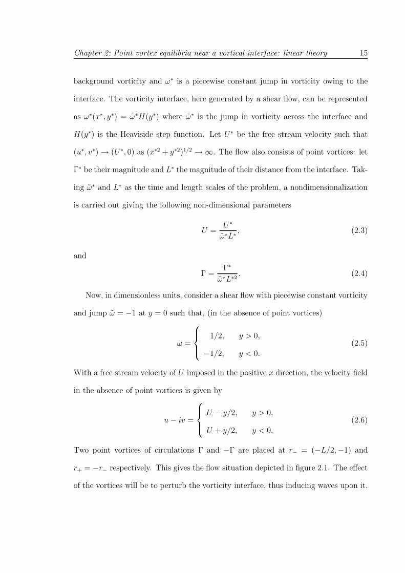
Two point vortices of circulations Γ and −Γ are placed at r− = (−L/2,−1) and
r+ = −r− respectively. This gives the flow situation depicted in figure 2.1. The effect
of the vortices will be to perturb the vorticity interface, thus inducing waves upon it.
Chapter 2: Point vortex equilibria near a vortical interface: linear theory 16
Now consider the initial unperturbed shear flow. If at some initial time the vortices
are then ‘turned’ on, this will result in some fluid being moved from y < 0 into y > 0
and vice versa. In two dimensions, the scalar vorticity associated with each fluid
particle is conserved. Therefore, the problem can be viewed as the initial shear flow
along with additional regions of vorticity with ∇2ψ = −1 when fluid has crossed from
y < 0 into y > 0, and ∇2ψ = 1 when fluid has crossed from y > 0 into y < 0.
In this section, linear theory is used to construct a non-radiating solution such that
the velocities at the vortices vanishes and the configuration remains stationary. The
parameters of the problem are Γ, L and U .
Figure 2.1: Sketch of the non-dimensional problem being considered. A shear flowis present with vorticity jump ω = −1 such that ω = 1/2 in y > 0 and ω = −1/2in y < 0 and the velocity is U at y = 0. Two vortices are placed at y = ±1 andseparated by a horizontal distance of L with circulations of ±Γ. The fluid disturbancealong the vorticity interface is labelled as y = η(x).
Denote the y-direction displacement of the vortical interface by y = η(x), where
Chapter 2: Point vortex equilibria near a vortical interface: linear theory 17
|η| ≪ 1. At the vorticity interface
D
Dt(y − η) = 0, (2.7)
which gives
v =Dη
Dt=∂η
∂t+ U · ∇η. (2.8)
For a stationary configuration ∂η/∂t = 0, therefore the linearised problem is to find
y = η(x), |η| ≪ 1, by solving
U∂η
∂x= v, on y = 0, (2.9)
where the vertical velocity, v, is given by
v =∂
∂x
− 1
2π
∫ ∞
−∞
∫ η(x′)
0
log[
(
(x− x′)2 + (y − y′)2)1/2]
dy′dx′
+Γ
2π
(
log[
(x+ L/2)2 + (y + 1)2]1/2 − log
[
(x− L/2)2 + (y − 1)2]1/2)
,
(2.10)
and U is the uniform background flow required to render the configuration stationary.
The integral term in (2.10) represents the contribution to the velocity owing to the
vorticity anomaly due to the displacement of y = η(x), whereas the final two terms
represent the two point vortices. The negative sign appears in front of the term owing
to the vorticity anomaly is, as mentioned above, such that ∇2ψ = −1 for y > 0. As
it is assumed that Γ > 0, the mutual self advection of the point vortices will result
in propagation in the negative x-direction. It is therefore expected that a stationary
configuration has U > 0. Consistent with linear dynamics, the approximation |η| ≪ 1
Chapter 2: Point vortex equilibria near a vortical interface: linear theory 18
and y = 0 are made in (2.10) giving
v = − 1
2π
∫ ∞
−∞
∫ η(x′)
0
x− x′
(x− x′)2 + y′2dy′dx′ +
Γ
2π
[
x+ L2
(
x+ L2
)2+ 1
− x− L2
(
x− L2
)2+ 1
]
= − 1
2π
∫ ∞
−∞
η(x′)
(x− x′)dx′ +
Γ
2π
[
x+ L2
(
x+ L2
)2+ 1
− x− L2
(
x− L2
)2+ 1
]
.
(2.11)
The Fourier Transform (FT) of v is given by
v =1
2π
∫ ∞
−∞
ve−ikxdx, (2.12)
where k is a wavenumber. Taking the FT of (2.11) yields
v =1
2π
∫ ∞
−∞
− 1
2π
∫ ∞
−∞
η(x′)
(x− x′)dx′ +
Γ
2π
[
x+ L2
(
x+ L2
)2+ 1
− x− L2
(
x− L2
)2+ 1
]
e−ikxdx
= − i
2sgnkη +
Γi
4πsgnke−|k|
(
eik L2 − e−ik L
2
)
.
(2.13)
Using (2.13) the FT of (2.9) is given by
Uikη =i
2sgnkη +
Γ
2πsgnke−|k| sin
(
kL
2
)
, (2.14)
where
η =1
2π
∫ ∞
−∞
ηe−ikxdx. (2.15)
Solving (2.14) for η gives
η = −Γi
2πsgnke−|k| sin(kL/2)
Uk − sgnk/2. (2.16)
Chapter 2: Point vortex equilibria near a vortical interface: linear theory 19
The dispersion relation for interfacial waves, following the analysis of Bell (1990) is
given by
σ = Uk − 1
2sgn k, (2.17)
where σ is the frequency. The phase and group velocities are
cp = U − 1
2|k| , cg = U − δ(k), (2.18)
where δ is the delta function. When U = 1/2|k| (2.16) has a simple pole and a steady
wavetrain forms downstream of the vortices and this, in general occurs for all U > 0.
In order for a stable configuration to exist it is required that this wave train vanishes.
Physically, this is equivalent to demanding that the wave trains due to each point
vortex destructively interfere. For this to be the case it is required that the simple
pole of (2.16) located at k = 1/2U vanishes. Setting L/2U = 2nπ, n = 0, 1, 2, ...,
this pole does indeed vanish and hence no wavetrain is located downstream of the
vortices, since from (2.16)
limk→1/2U
sin(2nπkU)
Uk − 1/2= (−1)n2nπ, n = 0, 1, 2, . . . . (2.19)
In the results that follow, n is set to n = 1 giving L = 4πU , the case where the
vortices are at their smallest horizontal separation. The contour shape is determined
by taking the inverse FT of equation (2.14) given by
η(x) =
∫ ∞
−∞
ηeikxdk, (2.20)
and therefore
η(x) = −Γi
2π
∫ ∞
−∞
sgnke−|k| sin(2kUπ)
Uk − sgnk/(2)eikxdk =
Γ
πU
∫ ∞
0
e−k sin(2kUπ) sin(kx)
k − 1/(2U)dk.
(2.21)
Chapter 2: Point vortex equilibria near a vortical interface: linear theory 20
Plotting (2.21) gives a contour which is anti-symmetric about x = 0 whose shape is
determined by U and Γ. The integral is computed numerically using a fourth order
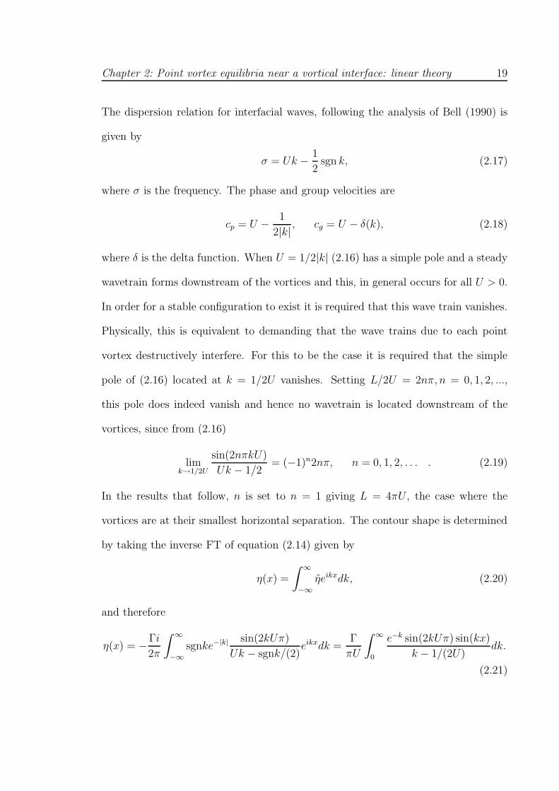
Runge-Kutta method for various values of x. Figure 2.2 shows η(x)/Γ for U = 1.0
and U = 0.187.
Figure 2.2: Profiles of η(x) given by (2.21) (normalised by Γ) with the non-radiatingcondition L = 4πU ; the solid line represents U = 1.0 and the dashed line U = 0.1876.
For a stationary configuration to be possible is also required that the x and y
velocities at both point vortices, induced by the contour and the other point vortex,
vanish for some values of U and Γ. In general the y-direction velocity at a position
(x, y) due to a point vortex with circulation γ at a position (a, b) is given by
v =∂
∂x
γ
2πlog[
(x− a)2 + (y − b)2]
12 . (2.22)
In the system under consideration γ = Γ at −L/2 and γ = −Γ at L/2. Owing to the
anti-symmetry of the problem, the y-direction velocity induced at each point vortex
Chapter 2: Point vortex equilibria near a vortical interface: linear theory 21
due to the other point vortex is, using L = 4πU , given by
vloc =UΓ
2(1 + (2πU)2). (2.23)
The y-direction velocity at each point vortex induced by the vorticity anomalies due
to the displaced contour is given by
vc = − 1
2π
∫ ∞
−∞
η(x′)(±L/2 − x′)
(±L/2 − x′)2 + 1dx′,
=Γi
4π2U
∫ ∞
−∞
∫ ∞
−∞
sgnke−|k| sin(2kUπ)eikx′
k − sgnk2U
(±L/2 − x′)
(±L/2 − x′)2 + 1dx′dk.
(2.24)
Using the substitutions ζ = L/2 + x′ when r = r− and ζ = −L/2 + x′ when r = r+
yields
vc =Γ
4πU
∫ ∞
−∞
e−|k| sin(2kUπ)
k − sgnk2U
e−|k|e∓ikL/2dk,
=Γ
2πU
∫ ∞
0
e−2k
k − 12U
sin(2kUπ) cos
(
kL
2
)
dk,
=Γ
4πU
∫ ∞
0
e−2k
k − 12U
sin(4kUπ)dk.
(2.25)
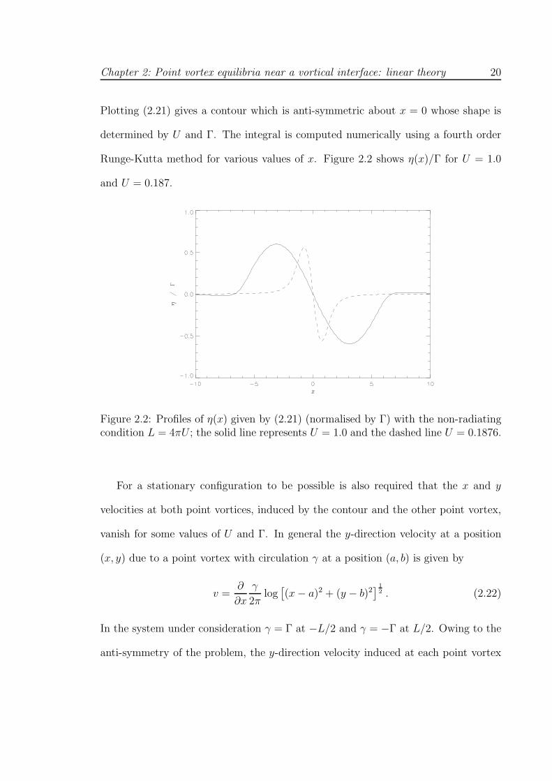
Here, U is positive and hence the vortices will have zero velocity in the y-direction
if (2.23)+(2.25)= 0. Figure 2.3 shows plots of vloc(x)/Γ and −vc(x)/Γ for various
values of U . The condition that (2.23)+(2.25)= 0 is satisfied for U = US ≈ 0.1876.
It has been shown that for this pair of vortices it is possible to impose a specific
US and L(= 4πUS) such that the vertical velocity at the vortices vanishes. It now
remains to resolve the condition that renders the vortices stationary in the horizontal
Chapter 2: Point vortex equilibria near a vortical interface: linear theory 22
Figure 2.3: Plot of −vc(x)/Γ (solid line) and vloc(x)/Γ (dashed line) (vertical axis)against U (horizontal axis).
direction. Now consider the x-direction velocities at each point vortex due to the
other vortex and the contour. The x-direction velocity at a position (x, y) owing to
a vortex at (a, b) is given by
u = − ∂
∂y
γ
2πlog[
(x− a)2 + (y − b)2] 1
2 . (2.26)
Again, due to the anti-symmetry of the problem the x-direction velocities at both
vortices are equal and are given by
uloc = − Γ
4π(4π2U2 + 1). (2.27)
Horizontal velocities at the vortices owing to the contour are given by
uc =1
2π
∫ ∞
−∞
η(x′)(±1 − 0)
(±L/2 − x′)2 + 1dx′. (2.28)
Chapter 2: Point vortex equilibria near a vortical interface: linear theory 23
Proceeding in the same way as determining (2.24), (2.28) gives
uc =Γ
2πU
∫ ∞
0
e−2k sin2(2πUk)
k − 12U
dk. (2.29)
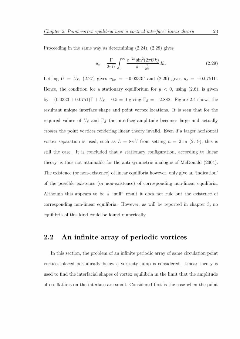
Letting U = US, (2.27) gives uloc = −0.0333Γ and (2.29) gives uc = −0.0751Γ.
Hence, the condition for a stationary equilibrium for y < 0, using (2.6), is given
by −(0.0333 + 0.0751)Γ + US − 0.5 = 0 giving ΓS = −2.882. Figure 2.4 shows the
resultant unique interface shape and point vortex locations. It is seen that for the
required values of US and ΓS the interface amplitude becomes large and actually
crosses the point vortices rendering linear theory invalid. Even if a larger horizontal
vortex separation is used, such as L = 8πU from setting n = 2 in (2.19), this is
still the case. It is concluded that a stationary configuration, according to linear
theory, is thus not attainable for the anti-symmetric analogue of McDonald (2004).
The existence (or non-existence) of linear equilibria however, only give an ‘indication’
of the possible existence (or non-existence) of corresponding non-linear equilibria.
Although this appears to be a “null” result it does not rule out the existence of
corresponding non-linear equilibria. However, as will be reported in chapter 3, no
equilibria of this kind could be found numerically.
2.2 An infinite array of periodic vortices
In this section, the problem of an infinite periodic array of same circulation point
vortices placed periodically below a vorticity jump is considered. Linear theory is
used to find the interfacial shapes of vortex equilibria in the limit that the amplitude
of oscillations on the interface are small. Considered first is the case when the point
Chapter 2: Point vortex equilibria near a vortical interface: linear theory 24
Figure 2.4: Profiles of η(x) with US = 0.1876 and ΓS = −2.882. The horizontalvortex equilibrium separation is given by L = 4πU and the two + signs mark thepoint vortex locations.
vortices are located in the irrotational region of the flow, followed by the case when
the vortices are located in the rotational region. The corresponding non-linear shapes
are found computationally in the following chapter.
2.2.1 Vortices in the irrotational flow region
The problem is initially considered in the plane and the vorticity jump is provided
by a shear flow. Periodicity is expected during the solution process. As seen in section
2.1 the flow is nondimensionalized using the vorticity jump, ω∗, and distance of the
vortices from the interface, L∗, as the time and length scales respectively. Consider a
Chapter 2: Point vortex equilibria near a vortical interface: linear theory 25
shear flow with a vorticity jump ω = −1 at y = 0 such that
ω =
1, y > 0,
0, y < 0.
(2.30)
With a free stream velocity of U imposed in the positive x direction, the velocity field
in the absence of point vortices is given by
u− iv =
U − y, y > 0,
U, y < 0.
(2.31)
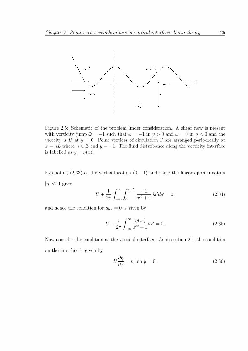
An infinite row of point vortices with circulations Γ are placed at rn = (nL,−1) where
n ∈ Z. Note that the vortices lie in the irrotational region. The interfacial shape,
η(x), will therefore be an even function on [−L/2, L/2] in order to ensure the vertical
velocity at any given point vortex vanishes, i.e. vloc = 0. In fact, the demand that
vloc = 0 necessarily implies this. The problem therefore consists of three parameters,
U , Γ and L. Unlike the problem considered in section 2.1, due to the periodicity of the
configuration, no radiation condition is required in the current problem. Therefore a
two parameter family of solutions is expected. A schematic of the problem is shown
in figure 2.5.
Consider the x-direction velocity at a point vortex. The stream function owing to
the vorticity anomalies (relative to the background vorticity distribution of the shear
flow) due to the displaced contour is given by
ψcontour =−1
2π
∫ ∞
−∞
∫ η(x′)
0
log[
(
(x− x′)2 + (y − y′)2)1/2]
dy′dx′. (2.32)
The condition to ensure uloc = 0 is given by
U +∂
∂y
1
2π
∫ ∞
−∞
∫ η(x′)
0
log[
(
(x− x′)2 + (y − y′)2)1/2]
dy′dx′ = 0. (2.33)
Chapter 2: Point vortex equilibria near a vortical interface: linear theory 26
Figure 2.5: Schematic of the problem under consideration. A shear flow is presentwith vorticity jump ω = −1 such that ω = −1 in y > 0 and ω = 0 in y < 0 and thevelocity is U at y = 0. Point vortices of circulation Γ are arranged periodically atx = nL where n ∈ Z and y = −1. The fluid disturbance along the vorticity interfaceis labelled as y = η(x).
Evaluating (2.33) at the vortex location (0,−1) and using the linear approximation
|η| ≪ 1 gives
U +1
2π
∫ ∞
−∞
∫ η(x′)
0
−1
x′2 + 1dx′dy′ = 0, (2.34)
and hence the condition for uloc = 0 is given by
U − 1
2π
∫ ∞
−∞
η(x′)
x′2 + 1dx′ = 0. (2.35)
Now consider the condition at the vortical interface. As in section 2.1, the condition
on the interface is given by
U∂η
∂x= v, on y = 0. (2.36)
Chapter 2: Point vortex equilibria near a vortical interface: linear theory 27
Thus
U∂η
∂x=
1
2π
∂
∂x
[
−∫ ∞
−∞
∫ η(x′)
0
log[
(
(x− x′)2 + (y − y′)2)1/2]
dy′dx′
+ Γ
∞∑
n=−∞
log[
(
(x+ nL)2 + (y + 1)2)
12
]
]
=1
2π
[
−∫ ∞
−∞
∫ η(x′)
0
x− x′
(x− x′)2 + (y − y′)2dx′dy′ + Γ
∞∑
n=−∞
x+ nL
(x+ nL)2 + (y + 1)2
]
,
(2.37)
where the sum represents the infinite periodic array of point vortices. Consistent with
linear theory, the approximations that |η| ≪ 1 and y = 0 are once again made in
(2.37) giving
U∂η
∂x=
1
2π
[
−∫ ∞
−∞
η(x′)
x− x′dx′ + Γ
∞∑
n=−∞
x+ nL
(x+ nl)2 + 1
]
. (2.38)
Now η(x) is a periodic function and can thus be represented as a Fourier series. As
mentioned at the beginning of the section, it is required that η(x) is an even function
on [−L/2, L/2] and therefore can be written as
η(x) =a0
2+
∞∑
k=1
ak cos
(
2kπx
L
)
, (2.39)
where the real constants ak are given by
ak =4
L
∫ L2
0
η(x) cos
(
2kπx
L
)
dx. (2.40)
The summation term on the right hand side of (2.38),∑∞
n=−∞x+kl
(x+kl)2+1, which is an
odd extension in[
0, L2
]
can also be written as a Fourier series. However, it simplifies
Chapter 2: Point vortex equilibria near a vortical interface: linear theory 28
the problem to use a different representation of this infinite series. Here, a suitable
form for the streamfunction along y = 0 of an infinite array of point vortices is given
by
ψloc(x, 0) =Γ
2πlog
∣
∣
∣
∣
β − cos
(
2πx
L
)∣
∣
∣
∣
12
, (2.41)
where β = cosh 2πL
(see Appendix B for details). The y-direction velocity at the
interface owing to the point vortices is thus given by
∂ψloc
∂x=
Γ
2L
sin(
2πxL
)
β − cos(
2πxL
) , (2.42)
and equating (2.42) to the summation on the right hand side of (2.38) gives
Γ
2π
∞∑
n=−∞
x+ kl
(x+ kl)2 + 1=
Γ
2L
sin(
2πxL
)
β − cos(
2πxL
) = g(x). (2.43)
The newly introduced function, g(x), can then be written as a Fourier series given by
g(x) =∞∑
k=1
bk sin
(
2πkx
L
)
, (2.44)
where
bk =Γ
2L
∫ L/2
0
sin(
2πxL
)
β − cos(
2πxL
) sin
(
2πkx
L
)
dx
=Γ
πL
∫ π
0
sin z sin kz
β − cos zdz =
Γ
Le−
2kπL .
(2.45)
Substituting (2.45) into equation (2.38) (and swapping n for k) gives
−∞∑
n=1
ak2nπU
Lsin
(
2nπx
L
)
=
− 1
4π
∫ ∞
−∞
a0
x− x′dx′ − 1
2π
∞∑
n=1
∫ ∞
−∞
an
cos(
2nπxL
)
x− x′dx′ +
∞∑
n=1
bn sin
(
2nπx
L
)
.
(2.46)
Chapter 2: Point vortex equilibria near a vortical interface: linear theory 29
It is now required to evaluate the two integrals (which are interpreted as Cauchy
principal value integrals) on the right hand side of (2.46). The results of these two
integrals are given below. The first integral yields
∫ ∞
−∞
a0
x− x′dx′ = 0. (2.47)
The second integral can be written as
∫ ∞
−∞
cos(
2nπx′
L
)
x− x′dx′ = ℜ
∫ ∞
−∞
ei 2nπx′
L
x− x′dx′. (2.48)
Substituting ζ = x′ − x gives
ℜ[
−ei 2nπxL
∫ ∞
−∞
ei 2nπζL
ζdζ ′
]
= π sin2nπx
L. (2.49)
Note that sgn(2nπ/L) = 1 has been used to obtain the result of (2.49). Substituting
(2.47) and (2.49) into (2.46) and equating coefficients of sin(2nπx/L) gives
an =bn
12− 2nπU
L
. (2.50)
Note that the form of (2.50) gives rise to the possibility of resonance of the nth
mode occurring when 2nπU/L ≃ 1/2. In such circumstances, there is potential for
an to become very large, resulting in large amplitude disturbances at the vorticity
interface. Linear theory is clearly not expected to be a good guide in systems where
such resonances occur.
In the studies of McDonald (2004) and Crowdy (1999, 2002a, b) it was shown that
the equilibria necessarily had zero circulation. This result does not appear naturally
in the present case. But, instead, it is insisted that the net circulation is zero. This
enables a0 to be determined. The zero net circulation case is, however, natural from
Chapter 2: Point vortex equilibria near a vortical interface: linear theory 30
a geophysical point of view: a meandering current sheds eddies so that the eddy
circulation and the vorticity deficit of the current must sum to zero. Considering the
region [−L/2, L/2], a net zero circulation equates to
Γ + γ
∫ L/2
−L/2
η(x) = 0. (2.51)
Here, the vorticity jump across the contour is −1 giving γ = −1 and thus
Γ −∫ L/2
−L/2
(
a0
2+ an cos
2nπx
L
)
dx = 0 (2.52)
yielding
a0 =2Γ
L. (2.53)
Equations (2.45) and (2.50) along with (2.35) and the result for a0, (2.53), can now
be used to calculate U and thus obtain the shape of the contour η. Substituting into
(2.35) gives
U − a0
4π
∫ ∞
−∞
dx′
1 + x′2−
∞∑
n=1
an
2π
∫ ∞
−∞
cos 2nπx′
L
1 + x′2dx′ = 0. (2.54)
Evaluating the integrals in (2.54) gives
∫ ∞
−∞
dx′
1 + x′2= π, (2.55)
and∫ ∞
−∞
cos 2nπx′
L
1 + x′2dx′ = πe−
2nπL . (2.56)
Substituting (2.55) and (2.56) along with (2.50) into (2.54) gives
2U − Γ
L+
∞∑
n=1
bn2nπU
L− 1
2
e−2nπL = 0, (2.57)
where the constants bn are given in (2.45). Substituting (2.50) for bn, (2.57) can be
written as
2U +Γ
L
(
∞∑
n=1
e−4nπL
2nπUL
− 12
− 1
)
= 0. (2.58)
Chapter 2: Point vortex equilibria near a vortical interface: linear theory 31
Values of U can thus be approximated by truncating (2.58) at some n = N and
solving the resultant (N + 1)th order polynomial in U . For a given value of Γ it is
therefore possible for U to take many different values. These possible values of U will
correspond to interfacial shapes of varying amplitudes and also, depending on Γ, some
values of U may be complex. Physically permissible solutions require U ∈ ℜ but also,
within this linear analysis only solutions leading to small amplitude interfacial shapes
are of interest. Note that the summation term on the left hand side of (2.58) decays
exponentially with increasing n. Therefore, to a good approximation, two roots of
U can be approximated by truncating the sum at n = 1 and solving the resulting
quadratic, or three roots by truncating at n = 2 and solving the resulting cubic and
so on.
From the perspective of linear analysis, the roots of U from (2.58) approximated
as a quadratic (or possibly cubic) will be of primary interest. This is due to the fact
that coefficients of higher powers of U decay rapidly and the roots corresponding to
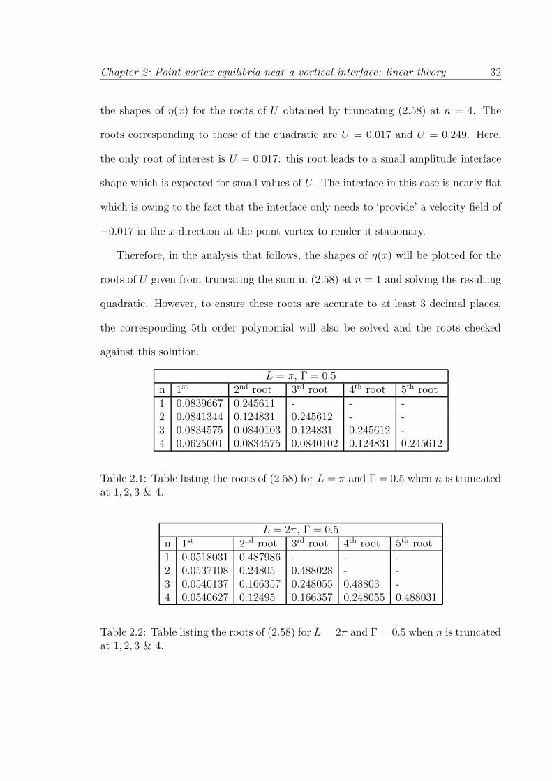
these higher powers of U will generally lead to resonance. Tables 2.1 and 2.2 show
the solutions of (2.58) for n truncated at 1,2,3,4 and Γ = 0.5 for L = π and L = 2π
respectively. Clearly, for any value of Γ, many distinct linear equilibria exist, one for
each possible value of U . However, from solving for the roots of U for many different
values of Γ and plotting the resulting interface shapes, it was seen that only the
roots corresponding to those of the quadratic gave solutions that were ‘possibly’ of
interest. For the values of Γ investigated, all other roots of U led to resonance or were
complex. (Note that ‘possibly’ is used here in the sense that roots of the quadratic
can also lead to large amplitude interface shapes). To illustrate this, figure 2.6 shows
Chapter 2: Point vortex equilibria near a vortical interface: linear theory 32
the shapes of η(x) for the roots of U obtained by truncating (2.58) at n = 4. The
roots corresponding to those of the quadratic are U = 0.017 and U = 0.249. Here,
the only root of interest is U = 0.017: this root leads to a small amplitude interface
shape which is expected for small values of U . The interface in this case is nearly flat
which is owing to the fact that the interface only needs to ‘provide’ a velocity field of
−0.017 in the x-direction at the point vortex to render it stationary.
Therefore, in the analysis that follows, the shapes of η(x) will be plotted for the
roots of U given from truncating the sum in (2.58) at n = 1 and solving the resulting
quadratic. However, to ensure these roots are accurate to at least 3 decimal places,
the corresponding 5th order polynomial will also be solved and the roots checked
against this solution.
L = π, Γ = 0.5n 1st 2nd root 3rd root 4th root 5th root1 0.0839667 0.245611 - - -2 0.0841344 0.124831 0.245612 - -3 0.0834575 0.0840103 0.124831 0.245612 -4 0.0625001 0.0834575 0.0840102 0.124831 0.245612
Table 2.1: Table listing the roots of (2.58) for L = π and Γ = 0.5 when n is truncatedat 1, 2, 3 & 4.
L = 2π, Γ = 0.5n 1st 2nd root 3rd root 4th root 5th root1 0.0518031 0.487986 - - -2 0.0537108 0.24805 0.488028 - -3 0.0540137 0.166357 0.248055 0.48803 -4 0.0540627 0.12495 0.166357 0.248055 0.488031
Table 2.2: Table listing the roots of (2.58) for L = 2π and Γ = 0.5 when n is truncatedat 1, 2, 3 & 4.
Chapter 2: Point vortex equilibria near a vortical interface: linear theory 33
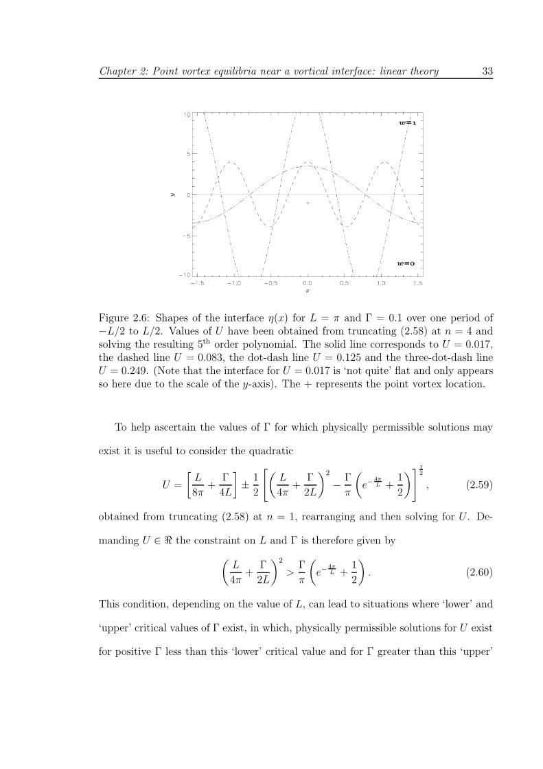
Figure 2.6: Shapes of the interface η(x) for L = π and Γ = 0.1 over one period of−L/2 to L/2. Values of U have been obtained from truncating (2.58) at n = 4 andsolving the resulting 5th order polynomial. The solid line corresponds to U = 0.017,the dashed line U = 0.083, the dot-dash line U = 0.125 and the three-dot-dash lineU = 0.249. (Note that the interface for U = 0.017 is ‘not quite’ flat and only appearsso here due to the scale of the y-axis). The + represents the point vortex location.
To help ascertain the values of Γ for which physically permissible solutions may
exist it is useful to consider the quadratic
U =
[
L
8π+
Γ
4L
]
± 1
2
[
(
L
4π+
Γ
2L
)2
− Γ
π
(
e−4πL +
1
2
)
]12
, (2.59)
obtained from truncating (2.58) at n = 1, rearranging and then solving for U . De-
manding U ∈ ℜ the constraint on L and Γ is therefore given by
(
L
4π+
Γ
2L
)2
>Γ
π
(
e−4πL +
1
2
)
. (2.60)
This condition, depending on the value of L, can lead to situations where ‘lower’ and
‘upper’ critical values of Γ exist, in which, physically permissible solutions for U exist
for positive Γ less than this ‘lower’ critical value and for Γ greater than this ‘upper’
Chapter 2: Point vortex equilibria near a vortical interface: linear theory 34
critical value. However, for Γ between these two critical values, solutions of U are
complex and are therefore not physical. Define
R(Γ, L) =
(
L4π
+ Γ2L
)2
Γπ
(
e−4πL + 1
2
) . (2.61)
Physically permissible (non-complex) solutions of U will therefore exist when R(Γ, L) ≥
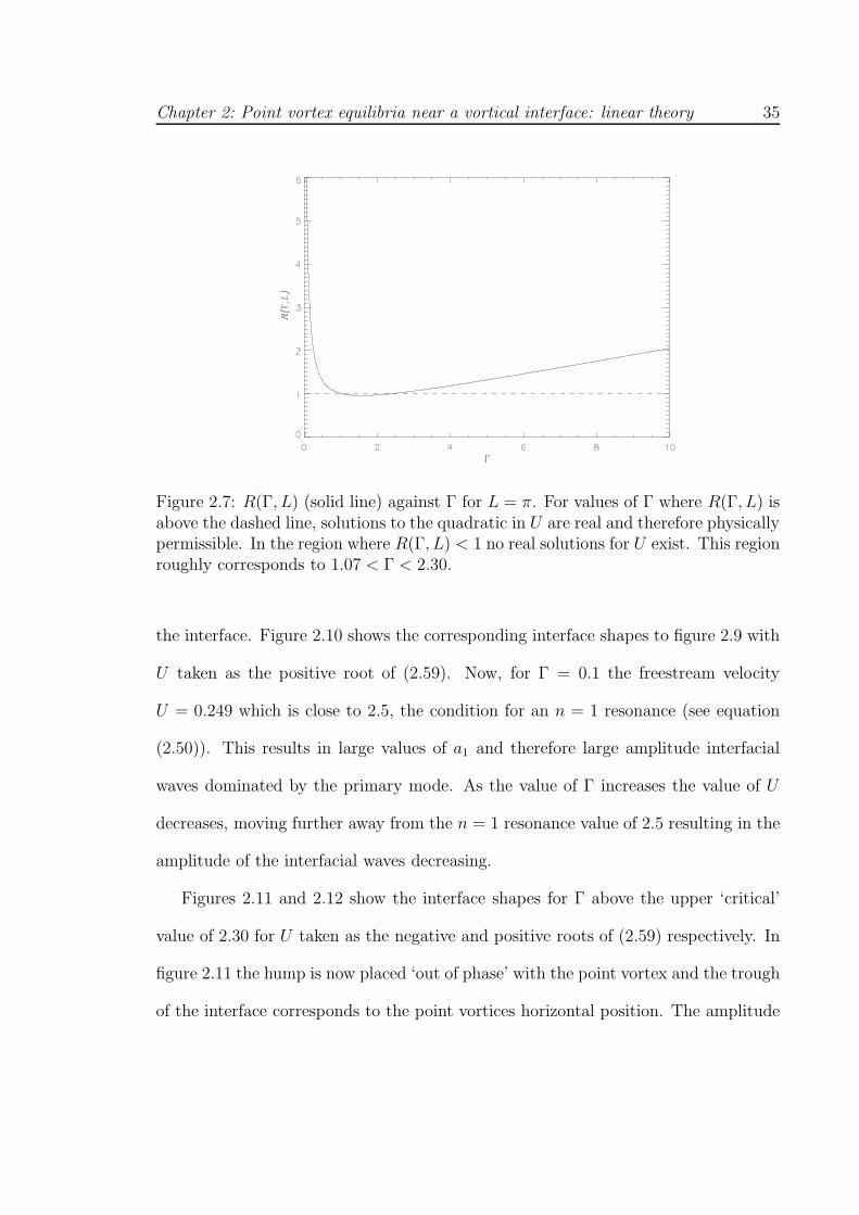
1. Figures 2.7 and 2.8 show plots of R(Γ, L) against Γ. Figure 2.7, in which L = π,
shows the two regions in which real solutions of (2.59) exist. In the region where
1.07 < Γ < 2.30 solutions of (2.59) will be complex and therefore not physically
permissible. For Γ > 0 and not within this region solutions of (2.59) will be real and
therefore physically permissible. Note however, that the larger the value of Γ, the
larger the expected amplitude of the interfacial waves. For waves of O(1) amplitude,
the validity of linear theory is brought into question and can be considered, at best,
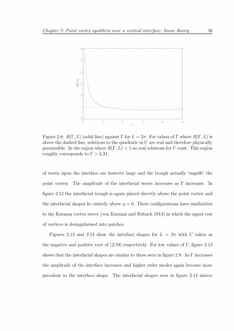
a ‘guide’ as to what non-linear equilibria may possibly exist. Figure 2.8 shows the
corresponding plot in which L = 2π. Here the region of ‘small’ Γ where R(Γ, L) > 1
is seen, but after R(Γ, L) initially falls below 1 it does not rise above 1 again until
Γ ≫ 1.
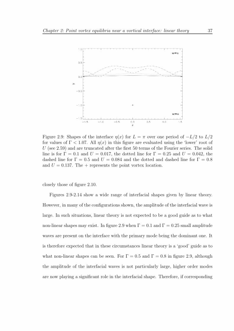
Figures 2.9-2.12 show examples of η(x) for various situations when L = π. When
evaluating η(x) the sum in equation (2.39) is truncated at k = 50 ensuring that
the accuracy of η(x) is determined by the accuracy of U and not by the truncation.
Figure 2.9 shows four interface shapes for Γ below the lower ‘critical’ value of 1.07
and the negative root of (2.59) taken for U . For Γ = 0.1 the interface has a small
amplitude hump symmetrically placed above the point vortex. The primary mode is
clearly the dominant mode in this circumstance. As Γ is increased the amplitude of
this hump also increases and the effect of higher order modes is clearly visible upon
Chapter 2: Point vortex equilibria near a vortical interface: linear theory 35
Figure 2.7: R(Γ, L) (solid line) against Γ for L = π. For values of Γ where R(Γ, L) isabove the dashed line, solutions to the quadratic in U are real and therefore physicallypermissible. In the region where R(Γ, L) < 1 no real solutions for U exist. This regionroughly corresponds to 1.07 < Γ < 2.30.
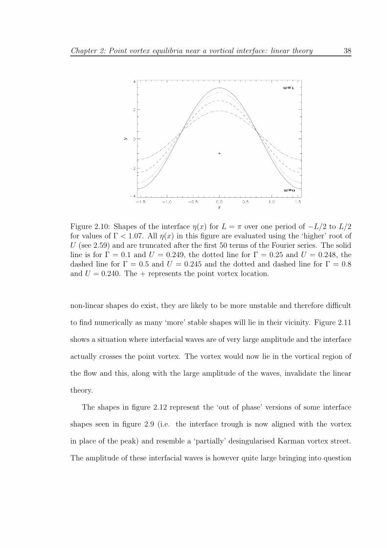
the interface. Figure 2.10 shows the corresponding interface shapes to figure 2.9 with
U taken as the positive root of (2.59). Now, for Γ = 0.1 the freestream velocity
U = 0.249 which is close to 2.5, the condition for an n = 1 resonance (see equation
(2.50)). This results in large values of a1 and therefore large amplitude interfacial
waves dominated by the primary mode. As the value of Γ increases the value of U
decreases, moving further away from the n = 1 resonance value of 2.5 resulting in the
amplitude of the interfacial waves decreasing.
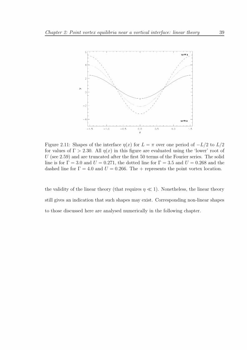
Figures 2.11 and 2.12 show the interface shapes for Γ above the upper ‘critical’
value of 2.30 for U taken as the negative and positive roots of (2.59) respectively. In
figure 2.11 the hump is now placed ‘out of phase’ with the point vortex and the trough
of the interface corresponds to the point vortices horizontal position. The amplitude
Chapter 2: Point vortex equilibria near a vortical interface: linear theory 36
Figure 2.8: R(Γ, L) (solid line) against Γ for L = 2π. For values of Γ where R(Γ, L) isabove the dashed line, solutions to the quadratic in U are real and therefore physicallypermissible. In the region where R(Γ, L) < 1 no real solutions for U exist. This regionroughly corresponds to Γ > 2.31.
of waves upon the interface are however large and the trough actually ‘engulfs’ the
point vortex. The amplitude of the interfacial waves increases as Γ increases. In
figure 2.12 the interfacial trough is again placed directly above the point vortex and
the interfacial shapes lie entirely above y = 0. These configurations have similarities
to the Karman vortex street (von Karman and Rubach 1913) in which the upper row
of vortices is desingularised into patches.
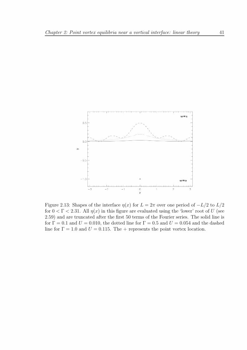
Figures 2.13 and 2.14 show the interface shapes for L = 2π with U taken as
the negative and positive root of (2.59) respectively. For low values of Γ, figure 2.13
shows that the interfacial shapes are similar to those seen in figure 2.9. As Γ increases
the amplitude of the interface increases and higher order modes again become more
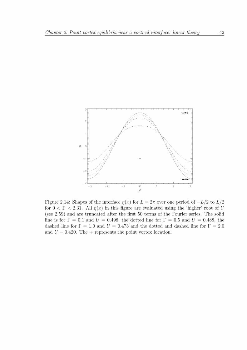
prevalent in the interface shape. The interfacial shapes seen in figure 2.14 mirror
Chapter 2: Point vortex equilibria near a vortical interface: linear theory 37
Figure 2.9: Shapes of the interface η(x) for L = π over one period of −L/2 to L/2for values of Γ < 1.07. All η(x) in this figure are evaluated using the ‘lower’ root ofU (see 2.59) and are truncated after the first 50 terms of the Fourier series. The solidline is for Γ = 0.1 and U = 0.017, the dotted line for Γ = 0.25 and U = 0.042, thedashed line for Γ = 0.5 and U = 0.084 and the dotted and dashed line for Γ = 0.8and U = 0.137. The + represents the point vortex location.
closely those of figure 2.10.
Figures 2.9-2.14 show a wide range of interfacial shapes given by linear theory.
However, in many of the configurations shown, the amplitude of the interfacial wave is
large. In such situations, linear theory is not expected to be a good guide as to what
non-linear shapes may exist. In figure 2.9 when Γ = 0.1 and Γ = 0.25 small amplitude
waves are present on the interface with the primary mode being the dominant one. It
is therefore expected that in these circumstances linear theory is a ‘good’ guide as to
what non-linear shapes can be seen. For Γ = 0.5 and Γ = 0.8 in figure 2.9, although
the amplitude of the interfacial waves is not particularly large, higher order modes
are now playing a significant role in the interfacial shape. Therefore, if corresponding
Chapter 2: Point vortex equilibria near a vortical interface: linear theory 38
Figure 2.10: Shapes of the interface η(x) for L = π over one period of −L/2 to L/2for values of Γ < 1.07. All η(x) in this figure are evaluated using the ‘higher’ root ofU (see 2.59) and are truncated after the first 50 terms of the Fourier series. The solidline is for Γ = 0.1 and U = 0.249, the dotted line for Γ = 0.25 and U = 0.248, thedashed line for Γ = 0.5 and U = 0.245 and the dotted and dashed line for Γ = 0.8and U = 0.240. The + represents the point vortex location.
non-linear shapes do exist, they are likely to be more unstable and therefore difficult
to find numerically as many ‘more’ stable shapes will lie in their vicinity. Figure 2.11
shows a situation where interfacial waves are of very large amplitude and the interface
actually crosses the point vortex. The vortex would now lie in the vortical region of
the flow and this, along with the large amplitude of the waves, invalidate the linear
theory.
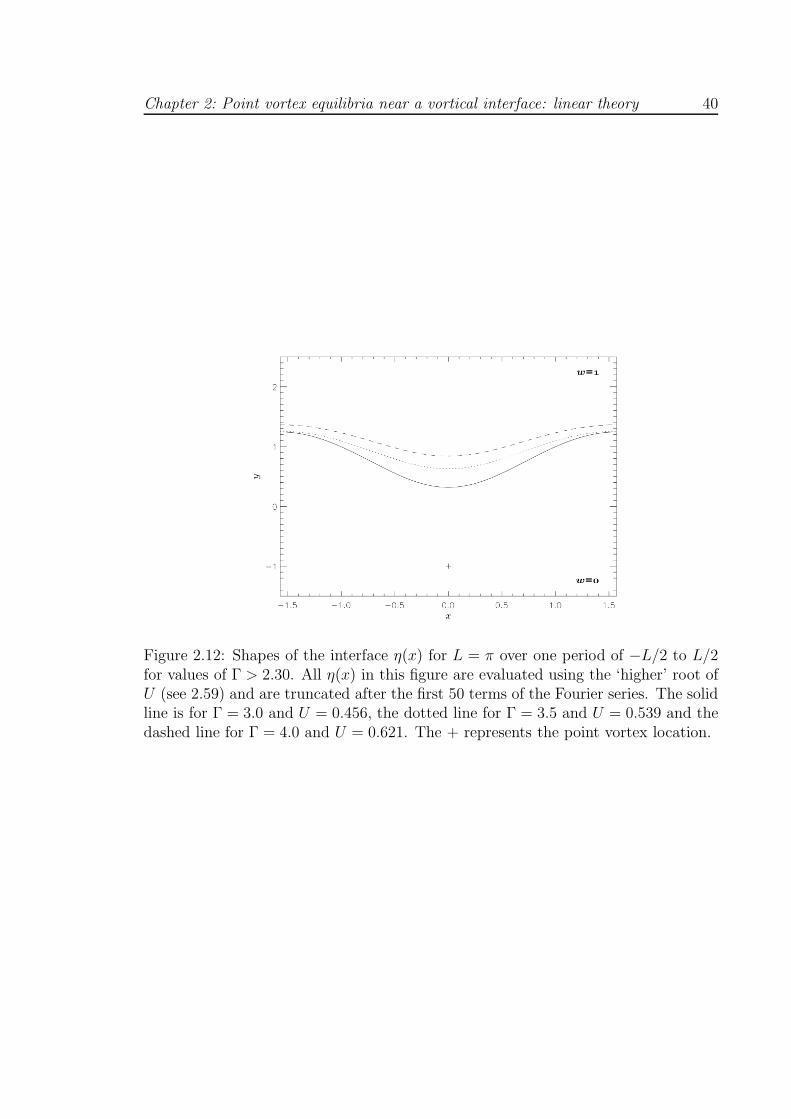
The shapes in figure 2.12 represent the ‘out of phase’ versions of some interface
shapes seen in figure 2.9 (i.e. the interface trough is now aligned with the vortex
in place of the peak) and resemble a ‘partially’ desingularised Karman vortex street.
The amplitude of these interfacial waves is however quite large bringing into question
Chapter 2: Point vortex equilibria near a vortical interface: linear theory 39
Figure 2.11: Shapes of the interface η(x) for L = π over one period of −L/2 to L/2for values of Γ > 2.30. All η(x) in this figure are evaluated using the ‘lower’ root ofU (see 2.59) and are truncated after the first 50 terms of the Fourier series. The solidline is for Γ = 3.0 and U = 0.271, the dotted line for Γ = 3.5 and U = 0.268 and thedashed line for Γ = 4.0 and U = 0.266. The + represents the point vortex location.
the validity of the linear theory (that requires η ≪ 1). Nonetheless, the linear theory
still gives an indication that such shapes may exist. Corresponding non-linear shapes
to those discussed here are analysed numerically in the following chapter.
Chapter 2: Point vortex equilibria near a vortical interface: linear theory 40
Figure 2.12: Shapes of the interface η(x) for L = π over one period of −L/2 to L/2for values of Γ > 2.30. All η(x) in this figure are evaluated using the ‘higher’ root ofU (see 2.59) and are truncated after the first 50 terms of the Fourier series. The solidline is for Γ = 3.0 and U = 0.456, the dotted line for Γ = 3.5 and U = 0.539 and thedashed line for Γ = 4.0 and U = 0.621. The + represents the point vortex location.
Chapter 2: Point vortex equilibria near a vortical interface: linear theory 41
Figure 2.13: Shapes of the interface η(x) for L = 2π over one period of −L/2 to L/2for 0 < Γ < 2.31. All η(x) in this figure are evaluated using the ‘lower’ root of U (see2.59) and are truncated after the first 50 terms of the Fourier series. The solid line isfor Γ = 0.1 and U = 0.010, the dotted line for Γ = 0.5 and U = 0.054 and the dashedline for Γ = 1.0 and U = 0.115. The + represents the point vortex location.
Chapter 2: Point vortex equilibria near a vortical interface: linear theory 42
Figure 2.14: Shapes of the interface η(x) for L = 2π over one period of −L/2 to L/2for 0 < Γ < 2.31. All η(x) in this figure are evaluated using the ‘higher’ root of U(see 2.59) and are truncated after the first 50 terms of the Fourier series. The solidline is for Γ = 0.1 and U = 0.498, the dotted line for Γ = 0.5 and U = 0.488, thedashed line for Γ = 1.0 and U = 0.473 and the dotted and dashed line for Γ = 2.0and U = 0.420. The + represents the point vortex location.
Chapter 2: Point vortex equilibria near a vortical interface: linear theory 43
2.2.2 Vortices in the rotational flow region
Consider a shear flow with vorticity jump ω = −1 at y = 0 such that the velocity
field in the absence of point vortices is given by
u− iv =
U, y > 0,
U + y, y < 0.
(2.62)
Compare this to (2.31): now the vortical region lies below y = 0. An infinite row of
periodic point vortices with circulation Γ are placed at rn = (nL,−1) (n ∈ Z) and are
now located in the rotational region of the flow. The analysis of this system is very
similar to that of section 2.2.1. The condition on the vortical interface is unchanged
and the condition to render uloc = 0 is modified to
U − 1 − 1
2π
∫ ∞
−∞
η(x′)
x′2 + 1dx′ = 0. (2.63)
Following the method of section 2.2.1, with the interface condition unchanged and
(2.35) modified to (2.63) leads to an equation for U given by
2(U − 1) +Γ
L
(
∞∑
n=1
e−4nπL
2nπUL
− 12
− 1
)
= 0. (2.64)
Truncating (2.64) for various n = N and solving the resultant (N + 1)th order poly-
nomial it is seen that once L is fixed, all but one root (for a given value for Γ) leads to
resonance. The root that does not lead to resonance is the only root with U > 1 and
corresponds to the positive root of the quadratic obtained from truncating (2.63) at
n = 1. Thus in the figures that follow, (2.64) was truncated at n = 4 to obtain a value
of the root with U > 1 accurate to at least three decimal places. Again, to gauge
for which values of Γ ‘useful’ solutions of (2.64) may exist it is useful to consider the
Chapter 2: Point vortex equilibria near a vortical interface: linear theory 44
function R(Γ, L). Truncating (2.64) at n = 1 and rearranging gives
U =
[
L
8π+
Γ
4L+
1
2
]
± 1
2
[
(
L
4π+
Γ
2L+ 1
)2
−(
Γ
πe−
4πL +
Γ
2π+L
π
)
]12
, (2.65)
and thus
R(Γ, L) =
(
L4π
+ Γ2L
+ 1)2
Γπe−
4πL + Γ
2π+ L
π
. (2.66)
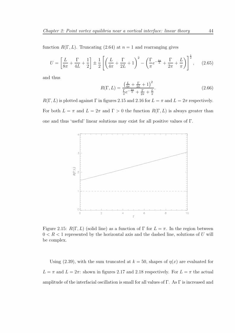
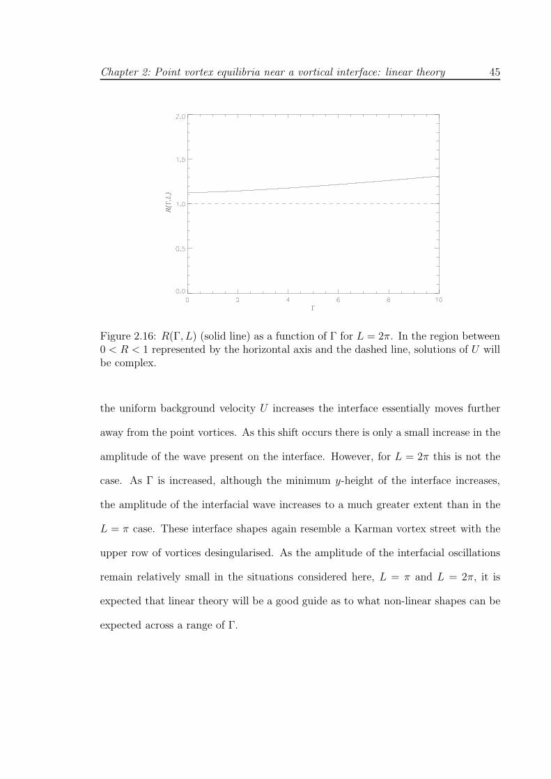
R(Γ, L) is plotted against Γ in figures 2.15 and 2.16 for L = π and L = 2π respectively.
For both L = π and L = 2π and Γ > 0 the function R(Γ, L) is always greater than
one and thus ‘useful’ linear solutions may exist for all positive values of Γ.
Figure 2.15: R(Γ, L) (solid line) as a function of Γ for L = π. In the region between0 < R < 1 represented by the horizontal axis and the dashed line, solutions of U willbe complex.
Using (2.39), with the sum truncated at k = 50, shapes of η(x) are evaluated for
L = π and L = 2π: shown in figures 2.17 and 2.18 respectively. For L = π the actual
amplitude of the interfacial oscillation is small for all values of Γ. As Γ is increased and
Chapter 2: Point vortex equilibria near a vortical interface: linear theory 45
Figure 2.16: R(Γ, L) (solid line) as a function of Γ for L = 2π. In the region between0 < R < 1 represented by the horizontal axis and the dashed line, solutions of U willbe complex.
the uniform background velocity U increases the interface essentially moves further
away from the point vortices. As this shift occurs there is only a small increase in the
amplitude of the wave present on the interface. However, for L = 2π this is not the
case. As Γ is increased, although the minimum y-height of the interface increases,
the amplitude of the interfacial wave increases to a much greater extent than in the
L = π case. These interface shapes again resemble a Karman vortex street with the
upper row of vortices desingularised. As the amplitude of the interfacial oscillations
remain relatively small in the situations considered here, L = π and L = 2π, it is
expected that linear theory will be a good guide as to what non-linear shapes can be
expected across a range of Γ.
Chapter 2: Point vortex equilibria near a vortical interface: linear theory 46
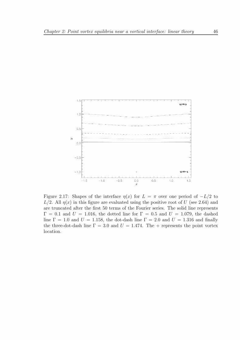
Figure 2.17: Shapes of the interface η(x) for L = π over one period of −L/2 toL/2. All η(x) in this figure are evaluated using the positive root of U (see 2.64) andare truncated after the first 50 terms of the Fourier series. The solid line representsΓ = 0.1 and U = 1.016, the dotted line for Γ = 0.5 and U = 1.079, the dashedline Γ = 1.0 and U = 1.158, the dot-dash line Γ = 2.0 and U = 1.316 and finallythe three-dot-dash line Γ = 3.0 and U = 1.474. The + represents the point vortexlocation.
Chapter 2: Point vortex equilibria near a vortical interface: linear theory 47
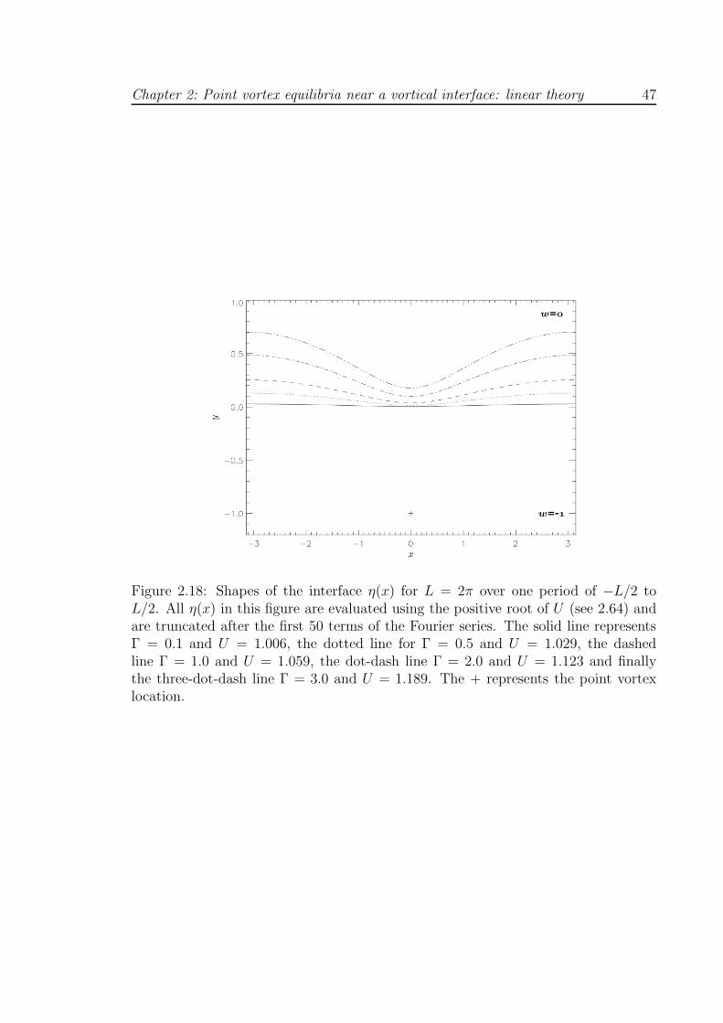
Figure 2.18: Shapes of the interface η(x) for L = 2π over one period of −L/2 toL/2. All η(x) in this figure are evaluated using the positive root of U (see 2.64) andare truncated after the first 50 terms of the Fourier series. The solid line representsΓ = 0.1 and U = 1.006, the dotted line for Γ = 0.5 and U = 1.029, the dashedline Γ = 1.0 and U = 1.059, the dot-dash line Γ = 2.0 and U = 1.123 and finallythe three-dot-dash line Γ = 3.0 and U = 1.189. The + represents the point vortexlocation.
Chapter 2: Point vortex equilibria near a vortical interface: linear theory 48
2.3 Vortex street in a shear flow
Similar to section 2.2, linear equilibria can also be constructed for the situation
where a vortex street (i.e. staggered rows of opposite-signed vortices) lies in a shear
flow. Here, the form of the shear flow is given by equations (2.5) and (2.6) i.e. in the
absence of point vortices
u =
U − y/2 y > 0,
U + y/2 y < 0.
(2.67)
Point vortices of equal but opposite circulations are periodically placed at (−L/4 ±
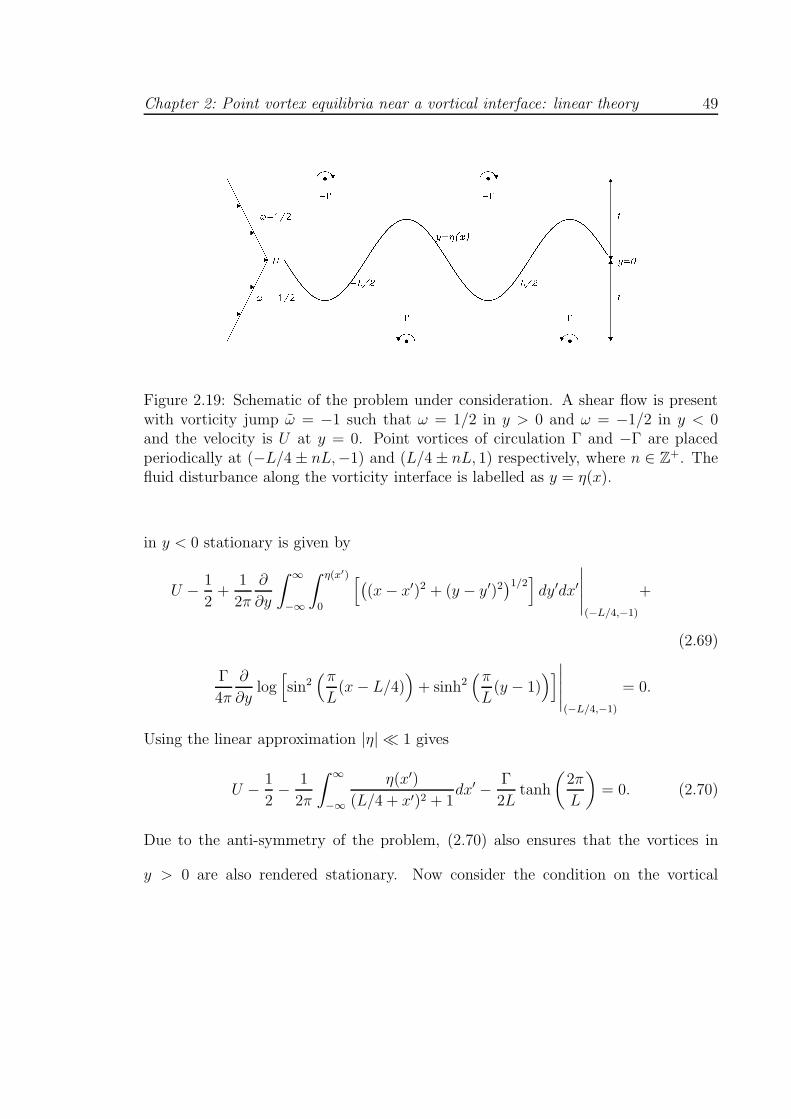
nL,−1) and (L/4 ± nL, 1), where n ∈ Z+. A schematic of the system is shown
in figure 2.19. Here, the circulation of the vortices, Γ, is not restricted to being
positive but instead can be of arbitrary sign. Due to the anti-symmetric nature
of the configuration, the interfacial contour, η(x), will also be anti-symmetric on
[−L/2, L/2]. This ensures that the y-direction velocity at the point vortices is zero.
The streamfunction for the interfacial disturbance is again given by equation
(2.32). The streamfunction ψpv owing to the periodic array of point vortices is
ψpv =γ
4πlog[
sin2(π
L(x− xloc)
)
+ sinh2(π
L(y − yloc)
)]
, (2.68)
where γ is the circulation of the vortices, L is the period of the configuration and
(xloc, yloc) position of one of the vortices. Here the region between L/2 and L/2 is
being considered and thus xloc ∈ [−L/2, L/2). The condition to render the vortices
Chapter 2: Point vortex equilibria near a vortical interface: linear theory 49
Figure 2.19: Schematic of the problem under consideration. A shear flow is presentwith vorticity jump ω = −1 such that ω = 1/2 in y > 0 and ω = −1/2 in y < 0and the velocity is U at y = 0. Point vortices of circulation Γ and −Γ are placedperiodically at (−L/4 ± nL,−1) and (L/4 ± nL, 1) respectively, where n ∈ Z
+. Thefluid disturbance along the vorticity interface is labelled as y = η(x).
in y < 0 stationary is given by
U − 1
2+
1
2π
∂
∂y
∫ ∞
−∞
∫ η(x′)
0
[
(
(x− x′)2 + (y − y′)2)1/2]
dy′dx′
∣
∣
∣
∣
∣
(−L/4,−1)
+
Γ
4π
∂
∂ylog[
sin2(π
L(x− L/4)
)
+ sinh2(π
L(y − 1)
)]
∣
∣
∣
∣
∣
(−L/4,−1)
= 0.
(2.69)
Using the linear approximation |η| ≪ 1 gives
U − 1
2− 1
2π
∫ ∞
−∞
η(x′)
(L/4 + x′)2 + 1dx′ − Γ
2Ltanh
(
2π
L
)
= 0. (2.70)
Due to the anti-symmetry of the problem, (2.70) also ensures that the vortices in
y > 0 are also rendered stationary. Now consider the condition on the vortical
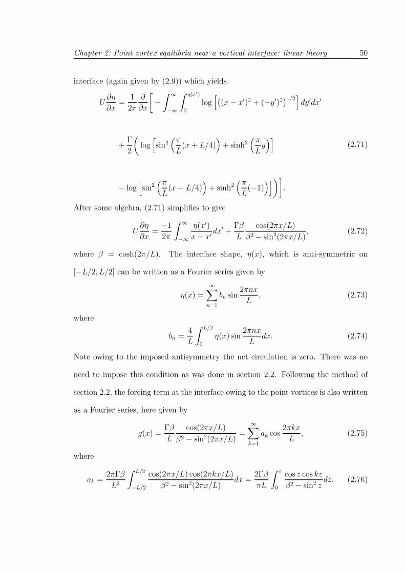
Chapter 2: Point vortex equilibria near a vortical interface: linear theory 50
interface (again given by (2.9)) which yields
U∂η
∂x=
1
2π
∂
∂x
[
−∫ ∞
−∞
∫ η(x′)
0
log[
(
(x− x′)2 + (−y′)2)1/2]
dy′dx′
+Γ
2
(
log[
sin2(π
L(x+ L/4)
)
+ sinh2(π
Ly)]
− log[
sin2(π
L(x− L/4)
)
+ sinh2(π
L(−1)
)]
)]
.
(2.71)
After some algebra, (2.71) simplifies to give
U∂η
∂x=
−1
2π
∫ ∞
−∞
η(x′)
x− x′dx′ +
Γβ
L
cos(2πx/L)
β2 − sin2(2πx/L), (2.72)
where β = cosh(2π/L). The interface shape, η(x), which is anti-symmetric on
[−L/2, L/2] can be written as a Fourier series given by
η(x) =∞∑
n=1
bn sin2πnx
L, (2.73)
where
bn =4
L
∫ L/2
0
η(x) sin2πnx
Ldx. (2.74)
Note owing to the imposed antisymmetry the net circulation is zero. There was no
need to impose this condition as was done in section 2.2. Following the method of
section 2.2, the forcing term at the interface owing to the point vortices is also written
as a Fourier series, here given by
g(x) =Γβ
L
cos(2πx/L)
β2 − sin2(2πx/L)=
∞∑
k=1
ak cos2πkx
L, (2.75)
where
ak =2πΓβ
L2
∫ L/2
−L/2
cos(2πx/L) cos(2πkx/L)
β2 − sin2(2πx/L)dx =
2Γβ
πL
∫ π
0
cos z cos kz
β2 − sin2 zdz. (2.76)
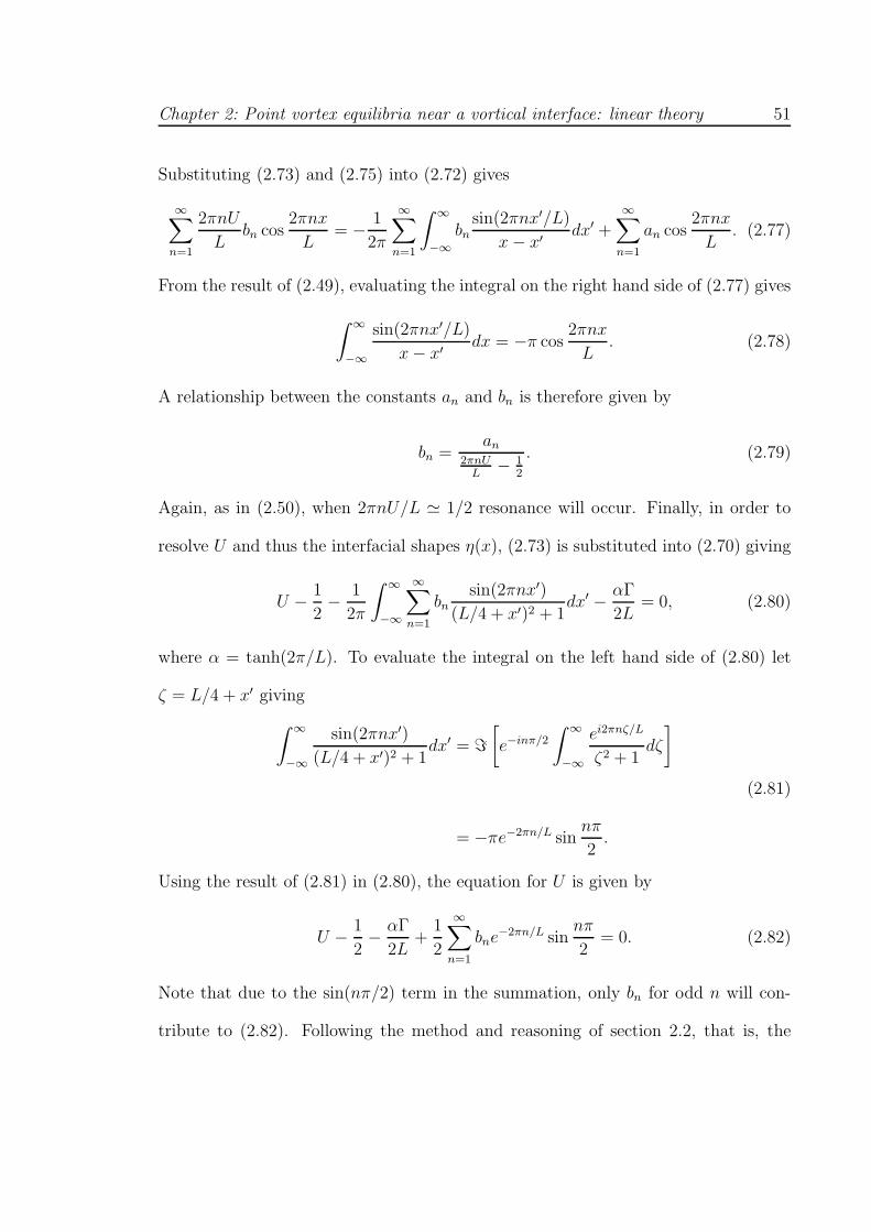
Chapter 2: Point vortex equilibria near a vortical interface: linear theory 51
Substituting (2.73) and (2.75) into (2.72) gives
∞∑
n=1
2πnU
Lbn cos
2πnx
L= − 1
2π
∞∑
n=1
∫ ∞
−∞
bnsin(2πnx′/L)
x− x′dx′ +
∞∑
n=1
an cos2πnx
L. (2.77)
From the result of (2.49), evaluating the integral on the right hand side of (2.77) gives
∫ ∞
−∞
sin(2πnx′/L)
x− x′dx = −π cos
2πnx
L. (2.78)
A relationship between the constants an and bn is therefore given by
bn =an
2πnUL
− 12
. (2.79)
Again, as in (2.50), when 2πnU/L ≃ 1/2 resonance will occur. Finally, in order to
resolve U and thus the interfacial shapes η(x), (2.73) is substituted into (2.70) giving
U − 1
2− 1
2π
∫ ∞
−∞
∞∑
n=1
bnsin(2πnx′)
(L/4 + x′)2 + 1dx′ − αΓ
2L= 0, (2.80)
where α = tanh(2π/L). To evaluate the integral on the left hand side of (2.80) let
ζ = L/4 + x′ giving
∫ ∞
−∞
sin(2πnx′)
(L/4 + x′)2 + 1dx′ = ℑ
[
e−inπ/2
∫ ∞
−∞
ei2πnζ/L
ζ2 + 1dζ
]
= −πe−2πn/L sinnπ
2.
(2.81)
Using the result of (2.81) in (2.80), the equation for U is given by
U − 1
2− αΓ
2L+
1
2
∞∑
n=1
bne−2πn/L sin
nπ
2= 0. (2.82)
Note that due to the sin(nπ/2) term in the summation, only bn for odd n will con-
tribute to (2.82). Following the method and reasoning of section 2.2, that is, the
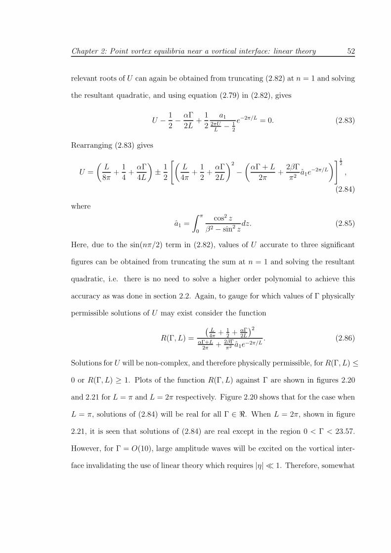
Chapter 2: Point vortex equilibria near a vortical interface: linear theory 52
relevant roots of U can again be obtained from truncating (2.82) at n = 1 and solving
the resultant quadratic, and using equation (2.79) in (2.82), gives
U − 1
2− αΓ
2L+
1
2
a1
2πUL
− 12
e−2π/L = 0. (2.83)
Rearranging (2.83) gives
U =
(
L
8π+
1
4+αΓ
4L
)
± 1
2
[
(
L
4π+
1
2+αΓ
2L
)2
−(
αΓ + L
2π+
2βΓ
π2a1e
−2π/L
)
]12
,
(2.84)
where
a1 =
∫ π
0
cos2 z
β2 − sin2 zdz. (2.85)
Here, due to the sin(nπ/2) term in (2.82), values of U accurate to three significant
figures can be obtained from truncating the sum at n = 1 and solving the resultant
quadratic, i.e. there is no need to solve a higher order polynomial to achieve this
accuracy as was done in section 2.2. Again, to gauge for which values of Γ physically
permissible solutions of U may exist consider the function
R(Γ, L) =
(
L4π
+ 12
+ αΓ2L
)2
αΓ+L2π
+ 2βΓπ2 a1e−2π/L
. (2.86)
Solutions for U will be non-complex, and therefore physically permissible, forR(Γ, L) ≤
0 or R(Γ, L) ≥ 1. Plots of the function R(Γ, L) against Γ are shown in figures 2.20
and 2.21 for L = π and L = 2π respectively. Figure 2.20 shows that for the case when
L = π, solutions of (2.84) will be real for all Γ ∈ ℜ. When L = 2π, shown in figure
2.21, it is seen that solutions of (2.84) are real except in the region 0 < Γ < 23.57.
However, for Γ = O(10), large amplitude waves will be excited on the vortical inter-
face invalidating the use of linear theory which requires |η| ≪ 1. Therefore, somewhat
Chapter 2: Point vortex equilibria near a vortical interface: linear theory 53
surprisingly, in this case (L = 2π) in the linear limit of small amplitude interfacial
waves, Γ is required to be negative.
Figure 2.20: R(Γ, L) (solid line) as a function of Γ for L = π. In the region betweenthe dashed lines, 0 < R(Γ, L) < 1, no real solutions of U exist. Here, solutions of Uare real for all Γ ∈ ℜ.
Using (2.76), (2.79) and (2.84) the interface shapes η(x) are determined. When
evaluating η(x), the sum in (2.73) was truncated at n = 50. Plots of η(x) for L = π
are shown in figures 2.22 and 2.23 for U evaluated taking the negative and positive
roots of (2.84) respectively. In figure 2.22, curves of η(x) are plotted for Γ = −4,
(for which U = −0.144) and Γ = −2, (for which U = 0.140). This leads to a
situation where the interface ‘sinks’ towards each point vortex. For both values of
Γ, the velocity due to U and the effect of the shear flow will be negative at each
point vortex (since U < 1/2 in both cases). Thus, for a stationary configuration the
velocity fields owing to the interfacial disturbance and the other point vortex need
to cancel exactly with this velocity field. Having the interface deform towards the
Chapter 2: Point vortex equilibria near a vortical interface: linear theory 54
Figure 2.21: R(Γ, L) (solid line) as a function of Γ for L = 2π. In the region betweenthe dashed lines, 0 < R(Γ, L) < 1, no real solutions of U exist. Here, solutions for Uwill be real for Γ not in the region 0 < Γ < 23.57.
point vortices results in the contributions to the velocity field from the interfacial
disturbance and the other vortex both being in the positive y-direction. For the case
when Γ = −1, the contribution from the other point vortex is comparatively large
and only a small amplitude disturbance at the interface is necessary to render the
configuration stationary. When Γ = −2 the other vortex contribution is smaller and a
larger amplitude interfacial disturbance is now required for a stationary configuration.
For L = π, when Γ is close to zero and when Γ > 0, evaluating equation (2.84) gives
U ≃ 0.25, the condition for an n = 1 resonance. Thus for Γ in this region the
amplitude of interfacial waves is large and linear theory is not applicable.
When evaluating U for L = π taking the positive root of (2.84), negative Γ
leads to an interfacial disturbance in the opposite direction to the case previously
considered, i.e. the interface moves ‘away’ from each point vortex. However, for
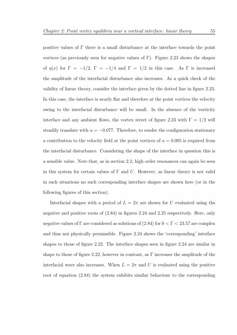
Chapter 2: Point vortex equilibria near a vortical interface: linear theory 55
positive values of Γ there is a small disturbance at the interface towards the point
vortices (as previously seen for negative values of Γ). Figure 2.23 shows the shapes
of η(x) for Γ = −1/2, Γ = −1/4 and Γ = 1/2 in this case. As Γ is increased
the amplitude of the interfacial disturbance also increases. As a quick check of the
validity of linear theory, consider the interface given by the dotted line in figure 2.23.
In this case, the interface is nearly flat and therefore at the point vortices the velocity
owing to the interfacial disturbance will be small. In the absence of the vorticity
interface and any ambient flows, the vortex street of figure 2.23 with Γ = 1/2 will
steadily translate with u = −0.077. Therefore, to render the configuration stationary
a contribution to the velocity field at the point vortices of u = 0.005 is required from
the interfacial disturbance. Considering the shape of the interface in question this is
a sensible value. Note that, as in section 2.2, high order resonances can again be seen
in this system for certain values of Γ and U . However, as linear theory is not valid
in such situations no such corresponding interface shapes are shown here (or in the
following figures of this section).
Interfacial shapes with a period of L = 2π are shown for U evaluated using the
negative and positive roots of (2.84) in figures 2.24 and 2.25 respectively. Here, only
negative values of Γ are considered as solutions of (2.84) for 0 < Γ < 23.57 are complex
and thus not physically permissible. Figure 2.24 shows the ‘corresponding’ interface
shapes to those of figure 2.22. The interface shapes seen in figure 2.24 are similar in
shape to those of figure 2.22, however in contrast, as Γ increases the amplitude of the
interfacial wave also increases. When L = 2π and U is evaluated using the positive
root of equation (2.84) the system exhibits similar behaviour to the corresponding
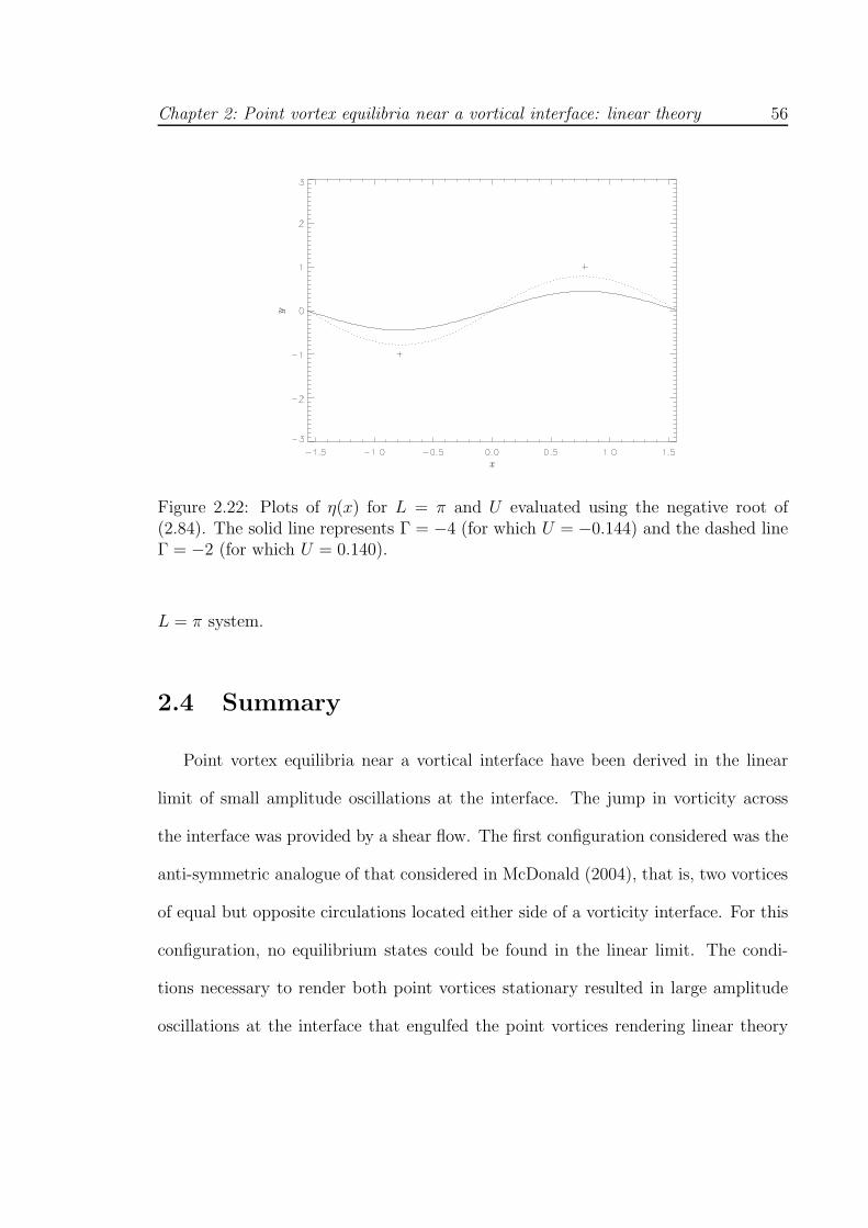
Chapter 2: Point vortex equilibria near a vortical interface: linear theory 56
Figure 2.22: Plots of η(x) for L = π and U evaluated using the negative root of(2.84). The solid line represents Γ = −4 (for which U = −0.144) and the dashed lineΓ = −2 (for which U = 0.140).
L = π system.
2.4 Summary
Point vortex equilibria near a vortical interface have been derived in the linear
limit of small amplitude oscillations at the interface. The jump in vorticity across
the interface was provided by a shear flow. The first configuration considered was the
anti-symmetric analogue of that considered in McDonald (2004), that is, two vortices
of equal but opposite circulations located either side of a vorticity interface. For this
configuration, no equilibrium states could be found in the linear limit. The condi-
tions necessary to render both point vortices stationary resulted in large amplitude
oscillations at the interface that engulfed the point vortices rendering linear theory
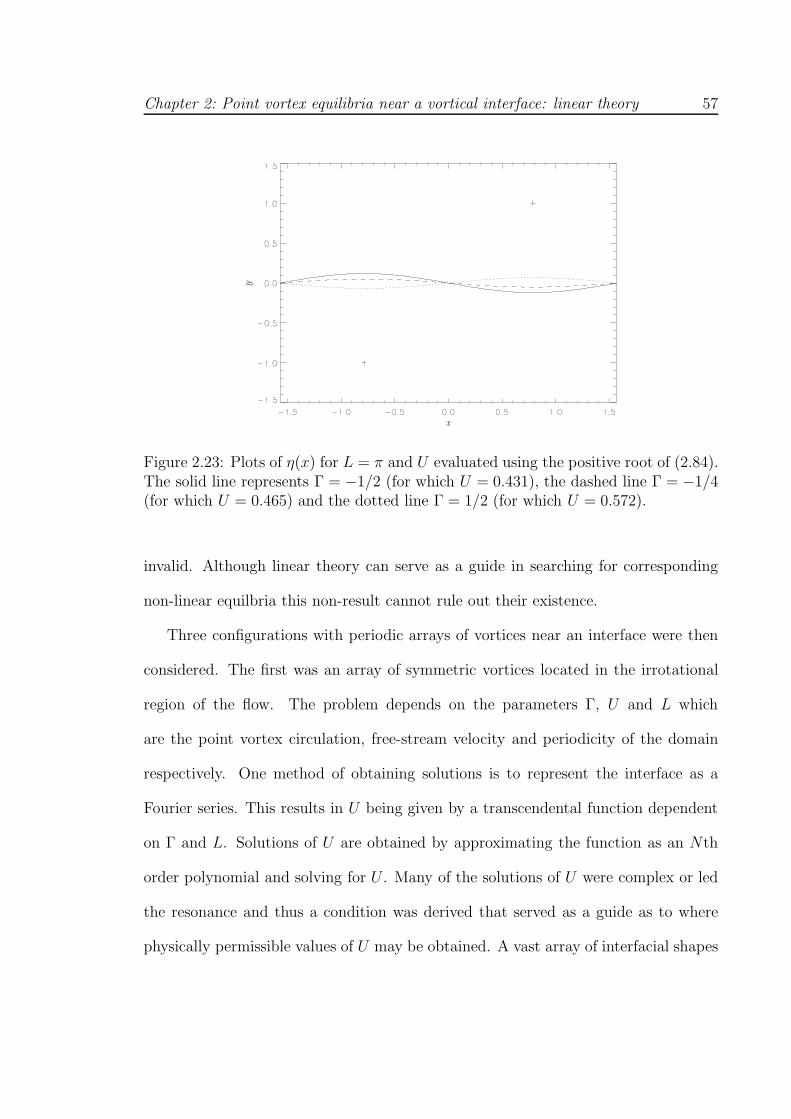
Chapter 2: Point vortex equilibria near a vortical interface: linear theory 57
Figure 2.23: Plots of η(x) for L = π and U evaluated using the positive root of (2.84).The solid line represents Γ = −1/2 (for which U = 0.431), the dashed line Γ = −1/4(for which U = 0.465) and the dotted line Γ = 1/2 (for which U = 0.572).
invalid. Although linear theory can serve as a guide in searching for corresponding
non-linear equilbria this non-result cannot rule out their existence.
Three configurations with periodic arrays of vortices near an interface were then
considered. The first was an array of symmetric vortices located in the irrotational
region of the flow. The problem depends on the parameters Γ, U and L which
are the point vortex circulation, free-stream velocity and periodicity of the domain
respectively. One method of obtaining solutions is to represent the interface as a
Fourier series. This results in U being given by a transcendental function dependent
on Γ and L. Solutions of U are obtained by approximating the function as an Nth
order polynomial and solving for U . Many of the solutions of U were complex or led
the resonance and thus a condition was derived that served as a guide as to where
physically permissible values of U may be obtained. A vast array of interfacial shapes
Chapter 2: Point vortex equilibria near a vortical interface: linear theory 58
Figure 2.24: Plots of η(x) for L = 2π and U evaluated using the negative root of(2.84). The solid line represents Γ = −1 (for which U = 0.320) and the dashed lineΓ = −0.1 (for which U = 0.450).
exist for the possible values of Γ, U and L. Many solutions lead to resonance and
large amplitude oscillations at the interface bringing into question the validity of
linear theory. However, for small Γ, some solutions are seen in which there exists a
small amplitude hump at the interface, placed symmetrically above the point vortex.
Also, some solutions were seen in which the interface amplitude remained relatively
small and higher order modes were playing a significant role in the interface shape.
Next, the above configuration with the vortices now placed in the rotational region
of the flow was considered. The method of solution closely parallels that of the
previous configuration. Solutions in which linear theory is expected to be a good
guide now have a hump at the interface placed out of phase with the point vortex,
resembling a Von-Karman vortex street one row of vortices desingularised. For small
L, interface shapes tended to be higher and flatter i.e. the interface would have a
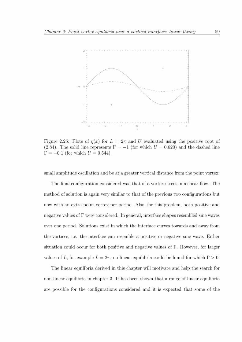
Chapter 2: Point vortex equilibria near a vortical interface: linear theory 59
Figure 2.25: Plots of η(x) for L = 2π and U evaluated using the positive root of(2.84). The solid line represents Γ = −1 (for which U = 0.620) and the dashed lineΓ = −0.1 (for which U = 0.544).
small amplitude oscillation and be at a greater vertical distance from the point vortex.
The final configuration considered was that of a vortex street in a shear flow. The
method of solution is again very similar to that of the previous two configurations but
now with an extra point vortex per period. Also, for this problem, both positive and
negative values of Γ were considered. In general, interface shapes resembled sine waves
over one period. Solutions exist in which the interface curves towards and away from
the vortices, i.e. the interface can resemble a positive or negative sine wave. Either
situation could occur for both positive and negative values of Γ. However, for larger
values of L, for example L = 2π, no linear equilibria could be found for which Γ > 0.
The linear equilibria derived in this chapter will motivate and help the search for
non-linear equilibria in chapter 3. It has been shown that a range of linear equilibria
are possible for the configurations considered and it is expected that some of the
Chapter 2: Point vortex equilibria near a vortical interface: linear theory 60
possible non-linear equilibria will be similar in shape. Thus, initially, in chapter 3,
the linear equilibria derived here will be used to initialise the non-linear computations.
Chapter 3
Computation of non-linear
equilibria on a vortical interface
In this chapter the corresponding non-linear equilibria to those found in the linear
limit of small amplitude interfacial oscillations in chapter 2 are computed numeri-
cally. To examine these non-linear equilibria a numerical procedure based on that of
McDonald (2004) is used. In general, the procedure entails using Newton’s method
to iterate the vortical interface to a shape such that is has a constant value of the
streamfunction along it (i.e. the interface becomes a streamline) and the velocity at
all point vortices vanishes. In iterating the interface towards a streamline, the param-
eters Γ and U and, depending on the system under consideration, possibly an extra
parameter measuring the vortex separation will also be calculated. When calculating
symmetric equilibria (c.f. chapter 2.2) the vortex position will remain fixed and when
calculating anti-symmetric equilibria (c.f. chapter 2.3) the distance of the vortices
from the interface will remain fixed. The vorticity distributions under consideration
61
Chapter 3: Computation of non-linear equilibria on a vortical interface 62
are piecewise constant, enabling the use of a contour dynamics algorithm (Dritschel
(1989)) to calculate the velocity field owing to the vorticity interface. For the planar
anti-symmetric system considered in chapter 2.1, a planar contour dynamics algo-
rithm is used while for the systems considered in chapters 2.2 and 2.3, a cylindrical
(or singly periodic) contour dynamics algorithm is used to account for the periodicity
of the vortical interface. First, computations of equilibria for the periodic configu-
ration of chapter 2.2 are presented. Equilibria are first computed for the case when
the point vortices are situated in the non-rotational region of the flow and also for
when they are situated in the rotational region. Next, equilibria are computed for
the anti-symmetric periodic configuration of chapter 2.3. Finally, as noted in chapter
2, no non-linear equilibria for the planar anti-symmetric configuration of chapter 2.1
could be found and this is briefly discussed.
3.1 Periodic symmetric equilibria
In computing periodic equilibria a modified version of the cylindrical contour
dynamics algorithm outlined in Dritschel (1989) is used. The vorticity dynamics are
formulated on the surface of an infinitely long, unit radius cylinder (which corresponds
to the case when L = 2π in chapters 2.2 and 2.3). In the algorithm, velocity fields
owing to piecewise constant vorticity jumps are determined using three dimensional
Cartesian coordinates restricted to the surface of the cylinder. From these Cartesian
coordinates the corresponding surface cylindrical coordinates φ and z, where φ ∈
[0, 2π) is the azimuthal angle and z ∈ (−∞,∞) is the along cylinder axis coordinate,
are determined. Note that here, the radial coordinate, r, is always given by r = 1.
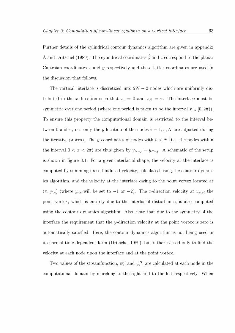
Chapter 3: Computation of non-linear equilibria on a vortical interface 63
Further details of the cylindrical contour dynamics algorithm are given in appendix
A and Dritschel (1989). The cylindrical coordinates φ and z correspond to the planar
Cartesian coordinates x and y respectively and these latter coordinates are used in
the discussion that follows.
The vortical interface is discretized into 2N − 2 nodes which are uniformly dis-
tributed in the x-direction such that x1 = 0 and xN = π. The interface must be
symmetric over one period (where one period is taken to be the interval x ∈ [0, 2π)).
To ensure this property the computational domain is restricted to the interval be-
tween 0 and π, i.e. only the y-location of the nodes i = 1, .., N are adjusted during
the iterative process. The y coordinates of nodes with i > N (i.e. the nodes within
the interval 0 < x < 2π) are thus given by yN+j = yN−j. A schematic of the setup
is shown in figure 3.1. For a given interfacial shape, the velocity at the interface is
computed by summing its self induced velocity, calculated using the contour dynam-
ics algorithm, and the velocity at the interface owing to the point vortex located at
(π, yloc) (where yloc will be set to −1 or −2). The x-direction velocity at uvort the
point vortex, which is entirely due to the interfacial disturbance, is also computed
using the contour dynamics algorithm. Also, note that due to the symmetry of the
interface the requirement that the y-direction velocity at the point vortex is zero is
automatically satisfied. Here, the contour dynamics algorithm is not being used in
its normal time dependent form (Dritschel 1989), but rather is used only to find the
velocity at each node upon the interface and at the point vortex.
Two values of the streamfunction, ψFi and ψB
i , are calculated at each node in the
computational domain by marching to the right and to the left respectively. When
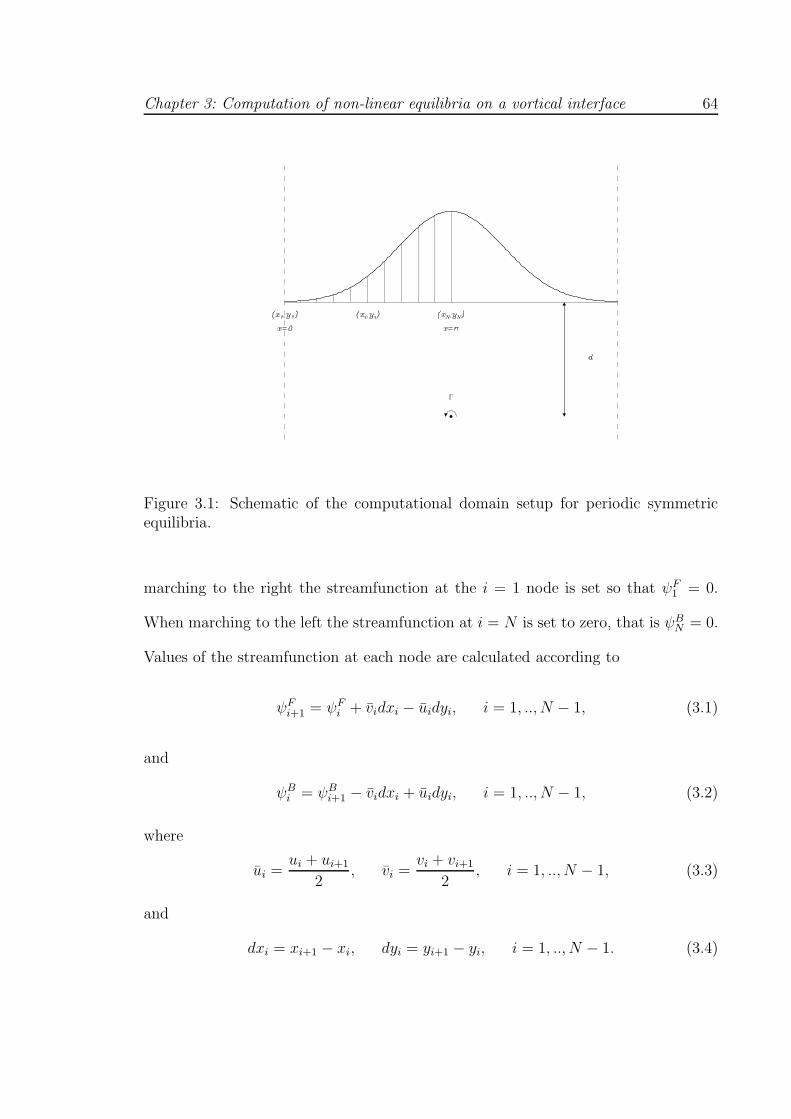
Chapter 3: Computation of non-linear equilibria on a vortical interface 64
Figure 3.1: Schematic of the computational domain setup for periodic symmetricequilibria.
marching to the right the streamfunction at the i = 1 node is set so that ψF1 = 0.
When marching to the left the streamfunction at i = N is set to zero, that is ψBN = 0.
Values of the streamfunction at each node are calculated according to
ψFi+1 = ψF
i + vidxi − uidyi, i = 1, .., N − 1, (3.1)
and
ψBi = ψB
i+1 − vidxi + uidyi, i = 1, .., N − 1, (3.2)
where
ui =ui + ui+1
2, vi =
vi + vi+1
2, i = 1, .., N − 1, (3.3)
and
dxi = xi+1 − xi, dyi = yi+1 − yi, i = 1, .., N − 1. (3.4)
Chapter 3: Computation of non-linear equilibria on a vortical interface 65
The streamfunction at each node is then the average of ψF and ψB, i.e.
ψi =ψF
i + ψBi
2. (3.5)
To find an equilibrium the values of yi and U are simultaneously adjusted so that, to
within some numerical tolerance, ψi = 0, i = 1, .., N , and the x-direction velocity at
the vortex, uvort = 0. By fixing the point vortex circulation, Γ, and the distance of
the vortex from the interface, the N + 1 unknowns y1, .., yN and U are given by the
N + 1 equations
ψi(y1, y2, .., yN , U) = 0, i = 1, .., N,
uvort(y1, y2, .., yN , U) = 0.
(3.6)
Equations (3.6) are solved using Newton’s method. For a given iteration, the nth
iteration say, the variables yj and U at the (n+1)th iteration are computed according
to
y(n+1)j = y
(n)j + ∆j , j = 1, .., N
U (n+1) = U (n) + ∆N+1,
(3.7)
where ∆j is the jth element of the vector solution of the (N + 1) × (N + 1) matrix
equation
N∑
j=1
∂ψ(n)i
∂yj∆j +
∂ψ(n)i
∂U∆N+1 = −ψ(n)
i , i = 1, .., N,
N∑
j=1
∂u(n)vort
∂yj
∆j +∂u
(n)vort
∂U∆N+1 = −u(n)
vort.
(3.8)
Chapter 3: Computation of non-linear equilibria on a vortical interface 66
The derivatives in (3.8) are computed numerically according to
∂f
∂l≈ f(l + δ) − f(l)
δ, (3.9)
using δ = 10−6. Therefore, in order to calculate the columns of the matrix, for a
configuration yj , U (j = 1, .., N), the contour dynamics algorithm is called to evaluate
the velocity at each node along with uvort. Knowing the velocity at each node enables
the streamfunction to be calculated using (3.5). The values yj at each node (or the
value of U when evaluating elements of the (N + 1)th row) are then varied by δ and
the contour dynamics algorithm is called to evaluate the new velocities, enabling the
evaluation of the new streamfunctions ψi(yj + δ) (i = 1, .., N) and uvort(yj + δ) (or
ψi(U + δ) and uvort(U + δ) when j = N + 1). Using the estimate of the derivative
given in (3.9) the columns of the matrix are hence evaluated. Finally, the matrix
equation (3.8) is solved by Gaussian elimination. Therefore, each iteration of the
above algorithm requires N + 2 calculations of the velocity field at all points, giving
a contour dynamics cost of (N + 2) × (N + 1). In addition, an (N + 1) × (N + 1)
matrix is inverted once per iteration.
In the following computations, the number of nodes in the computational domain
is set to N = 100, giving a resolution in the x-direction of δx = 0.0314. Increasing
the number of nodes within the computational domain (i.e. decreasing δx) results in
the algorithm converging to a slightly different steady state which, although different,
is nevertheless, a genuine equilibria. This is due to the fact that all nodes within the
computational domain are free to move in the y-direction and is not due to a lack of
resolution in the x-direction to obtain convergence. As all nodes are free to move in
the y-direction, it is possible for the entire interface to shift ‘upwards’ or ‘downwards’
Chapter 3: Computation of non-linear equilibria on a vortical interface 67
through the course of a simulation. This is equivalent to, say, altering the periodicity
of the domain in chapter 2.2 which, in the linear regime, can introduce a number
of possible new equilibrium shapes. Thus for a point vortex of fixed circulation at
some fixed distance below the y-axis it is expected that the algorithm will converge
to many distinct equilibria depending on the initial conditions used, i.e. depending
on the initial choice of interface shape and free stream velocity U . This is typical of
Newtonian iteration.
In order to monitor the convergence of the computed equilibria, values of both U
and the area of the interfacial disturbance are recorded and it is ensured that these
values have converged to at least six decimal places in all results that follow. This
level of convergence was generally realised within 50 iterations.
The lack of exact solutions for the non-linear equilibria inhibits an analytical inves-
tigation of their stability. Thus, to examine the stability, or robustness of computed
equilibria, they are then used as initial conditions in a fully non-linear time depen-
dent cylindrical contour dynamics code. A robust equilibrium is expected to remain
largely unchanged for a reasonable period of time. Conversely, if an equilibrium is
unstable, due to numerical perturbations it is expected to quickly lose coherence and
behave in a complicated manner. Some of the equilibria are tested in this way.
3.1.1 Point vortex in the irrotational flow region
Consider the configuration where the vortex is in the irrotational region of the
flow (chapter 2.2.1, figure 2.5). The linear equilibria computed in chapter 2.2.1 are
used to initialise the non-linear algorithm described above. For the case in chapter
Chapter 3: Computation of non-linear equilibria on a vortical interface 68
2.2.1 when L = π, this equates to multiplying all length scales by a factor of two and
consequently the point vortex circulation by a factor of four and U by a factor of two.
Figure 3.2 shows the non-linear equilibria computed with (Γ = 0.4, U0 = 0.034), (Γ =
1.0, U0 = 0.084) and (Γ = 2.0, U0 = 0.168) as initial conditions (where the brackets
have been introduced for ease of notation and indicate the pair of initial values used
in each case and U0 represents the value of U used to initialise the simulation. Note
that here, Γ remains fixed). These initial conditions correspond to three of the linear
equilibria shown in figure 2.9 ‘stretched’ into a domain with 2π periodicity. When
Γ = 0.4 and Γ = 1, through visual comparison, it is seen that the shapes of η(x)
correspond very closely to their linear counterparts of figure 2.9 (i.e. the equilibria
with (Γ = 0.1, U = 0.017) and (Γ = 0.25, U = 0.042) respectively). However, when
Γ = 2, the higher order modes present in the linear equilibria are clearly absent
in the ‘corresponding’ non-linear case; the shape of the interface is very similar to
when Γ = 0.4 or Γ = 1 but with a higher amplitude. This is not unexpected as,
as mentioned above, all interfacial nodes are free to move in the y-direction making
the algorithm more likely to converge to a more stable equilibrium without higher
order modes. Therefore, if non-linear equilibria in which higher order modes play a
significant role do exist, it is likely that a different algorithm is needed to find them.
Consequently, the constraints seen on the values of Γ that give physically permissible
U (i.e. 2.60 and 2.61) in the linear analysis are not observed here. Also, the equilibria
of chapter 2.2.1 with large amplitude interface oscillations, such as in figures 2.10 and
2.12, could not be realised numerically. In fact, the equilibria of figure 2.12 resemble
closely some of the non-linear equilibria computed when the point vortex is in the
Chapter 3: Computation of non-linear equilibria on a vortical interface 69
rotational region of the flow as will be seen in the following section.
When initialising the algorithm with the linear equilibria of chapter 2.2.1 with
L = 2π no corresponding non-linear equilibria could be found. In all cases the
algorithm would either diverge or converge to a result in which a great deal of noise
was present at the edges of the vortical interface. Equilibria could however be found
when the algorithm was initialised with the point vortex unit distance from a flat
interface. However, in such cases the interface would essentially move away from
the vortex to an equilibrium position in which the vertical separation of vortex and
interface was far greater than the initial unit distance. This resulted in equilibria
similar to those shown of figure 3.3 (whose computation is detailed below).
Figure 3.3 shows equilibria resulting from initialising the simulation with the vor-
tex at (π,−2) and a flat interface along y = 0 with (Γ = 4, U0 = 0.3), (Γ = 12, U0 =
0.5) and (Γ = 20, U0 = 0.6). In the three equilibria of figure 3.3 it is seen that the
node at x = 0 is at a location with y < 0. This was a common feature of equilibria
resulting from initialising the simulation with the vortex at (π,−2) for various initial
interface shapes. Another example of an initial interface shape used was a Gaussian
profile. Also, as noted previously, in simulations initiated with the vortex located
at (π,−1) and a flat interface along y = 0, the whole interface would often ‘lift up’
resulting in a vortex-interface separation similar to the separations seen in figure 3.3.
This seemingly preferential vortex-interface separation possibly gives some indication
of an optimum vortex-interface separation for stability. It should also be noted that
initialising simulations with a vortex of the same circulation but with different values
of U0 could lead to the algorithm converging to different equilibria. These equilibria
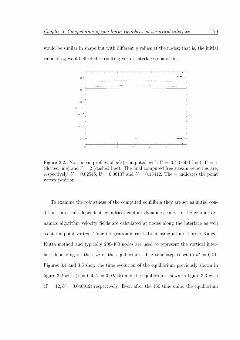
Chapter 3: Computation of non-linear equilibria on a vortical interface 70
would be similar in shape but with different y values at the nodes; that is, the initial
value of U0 would effect the resulting vortex-interface separation.
Figure 3.2: Non-linear profiles of η(x) computed with Γ = 0.4 (solid line), Γ = 1(dotted line) and Γ = 2 (dashed line). The final computed free stream velocities are,respectively, U = 0.02545, U = 0.06137 and U = 0.13412. The + indicates the pointvortex position.
To examine the robustness of the computed equilibria they are set as initial con-
ditions in a time dependent cylindrical contour dynamics code. In the contour dy-
namics algorithm velocity fields are calculated at nodes along the interface as well
as at the point vortex. Time integration is carried out using a fourth order Runge-
Kutta method and typically 200-400 nodes are used to represent the vortical inter-
face depending on the size of the equilibrium. The time step is set to dt = 0.01.
Figures 3.4 and 3.5 show the time evolution of the equilibrium previously shown in
figure 3.2 with (Γ = 0.4, U = 0.02545) and the equilibrium shown in figure 3.3 with
(Γ = 12, U = 0.040912) respectively. Even after the 150 time units, the equilibrium
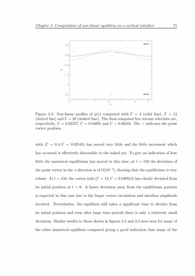
Chapter 3: Computation of non-linear equilibria on a vortical interface 71
Figure 3.3: Non-linear profiles of η(x) computed with Γ = 4 (solid line), Γ = 12(dotted line) and Γ = 20 (dashed line). The final computed free stream velocities are,respectively, U = 0.02357, U = 0.04091 and U = 0.00310. The + indicates the pointvortex position.
with (Γ = 0.4, U = 0.02545) has moved very little and the little movement which
has occurred is effectively discernible to the naked eye. To give an indication of how
little the numerical equilibrium has moved in this time, at t = 150 the deviation of
the point vortex in the x-direction is of O(10−4), showing that the equilibrium is very
robust. At t = 150, the vortex with (Γ = 12, U = 0.040912) has clearly deviated from
its initial position at t = 0. A faster deviation away from the equilibrium position
is expected in this case due to the larger vortex circulation and interface amplitude
involved. Nevertheless, the equilibria still takes a significant time to deviate from
its initial position and even after large time periods there is only a relatively small
deviation. Similar results to those shown in figures 3.2 and 3.3 were seen for many of
the other numerical equilibria computed giving a good indication that many of the
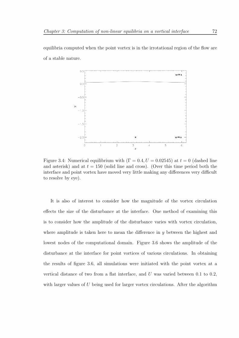
Chapter 3: Computation of non-linear equilibria on a vortical interface 72
equilibria computed when the point vortex is in the irrotational region of the flow are
of a stable nature.
Figure 3.4: Numerical equilibrium with (Γ = 0.4, U = 0.02545) at t = 0 (dashed lineand asterisk) and at t = 150 (solid line and cross). (Over this time period both theinterface and point vortex have moved very little making any differences very difficultto resolve by eye).
It is also of interest to consider how the magnitude of the vortex circulation
effects the size of the disturbance at the interface. One method of examining this
is to consider how the amplitude of the disturbance varies with vortex circulation,
where amplitude is taken here to mean the difference in y between the highest and
lowest nodes of the computational domain. Figure 3.6 shows the amplitude of the
disturbance at the interface for point vortices of various circulations. In obtaining
the results of figure 3.6, all simulations were initiated with the point vortex at a
vertical distance of two from a flat interface, and U was varied between 0.1 to 0.2,
with larger values of U being used for larger vortex circulations. After the algorithm
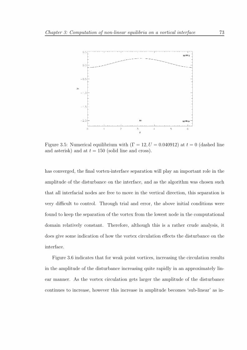
Chapter 3: Computation of non-linear equilibria on a vortical interface 73
Figure 3.5: Numerical equilibrium with (Γ = 12, U = 0.040912) at t = 0 (dashed lineand asterisk) and at t = 150 (solid line and cross).
has converged, the final vortex-interface separation will play an important role in the
amplitude of the disturbance on the interface, and as the algorithm was chosen such
that all interfacial nodes are free to move in the vertical direction, this separation is
very difficult to control. Through trial and error, the above initial conditions were
found to keep the separation of the vortex from the lowest node in the computational
domain relatively constant. Therefore, although this is a rather crude analysis, it
does give some indication of how the vortex circulation effects the disturbance on the
interface.
Figure 3.6 indicates that for weak point vortices, increasing the circulation results
in the amplitude of the disturbance increasing quite rapidly in an approximately lin-
ear manner. As the vortex circulation gets larger the amplitude of the disturbance
continues to increase, however this increase in amplitude becomes ‘sub-linear’ as in-
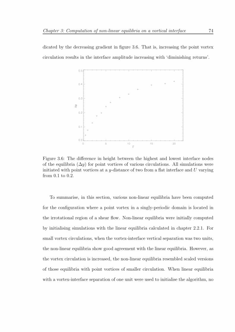
Chapter 3: Computation of non-linear equilibria on a vortical interface 74
dicated by the decreasing gradient in figure 3.6. That is, increasing the point vortex
circulation results in the interface amplitude increasing with ‘diminishing returns’.
Figure 3.6: The difference in height between the highest and lowest interface nodesof the equilibria (∆y) for point vortices of various circulations. All simulations wereinitiated with point vortices at a y-distance of two from a flat interface and U varyingfrom 0.1 to 0.2.
To summarise, in this section, various non-linear equilibria have been computed
for the configuration where a point vortex in a singly-periodic domain is located in
the irrotational region of a shear flow. Non-linear equilibria were initially computed
by initialising simulations with the linear equilibria calculated in chapter 2.2.1. For
small vortex circulations, when the vortex-interface vertical separation was two units,
the non-linear equilibria show good agreement with the linear equilibria. However, as
the vortex circulation is increased, the non-linear equilibria resembled scaled versions
of those equilibria with point vortices of smaller circulation. When linear equilibria
with a vortex-interface separation of one unit were used to initialise the algorithm, no
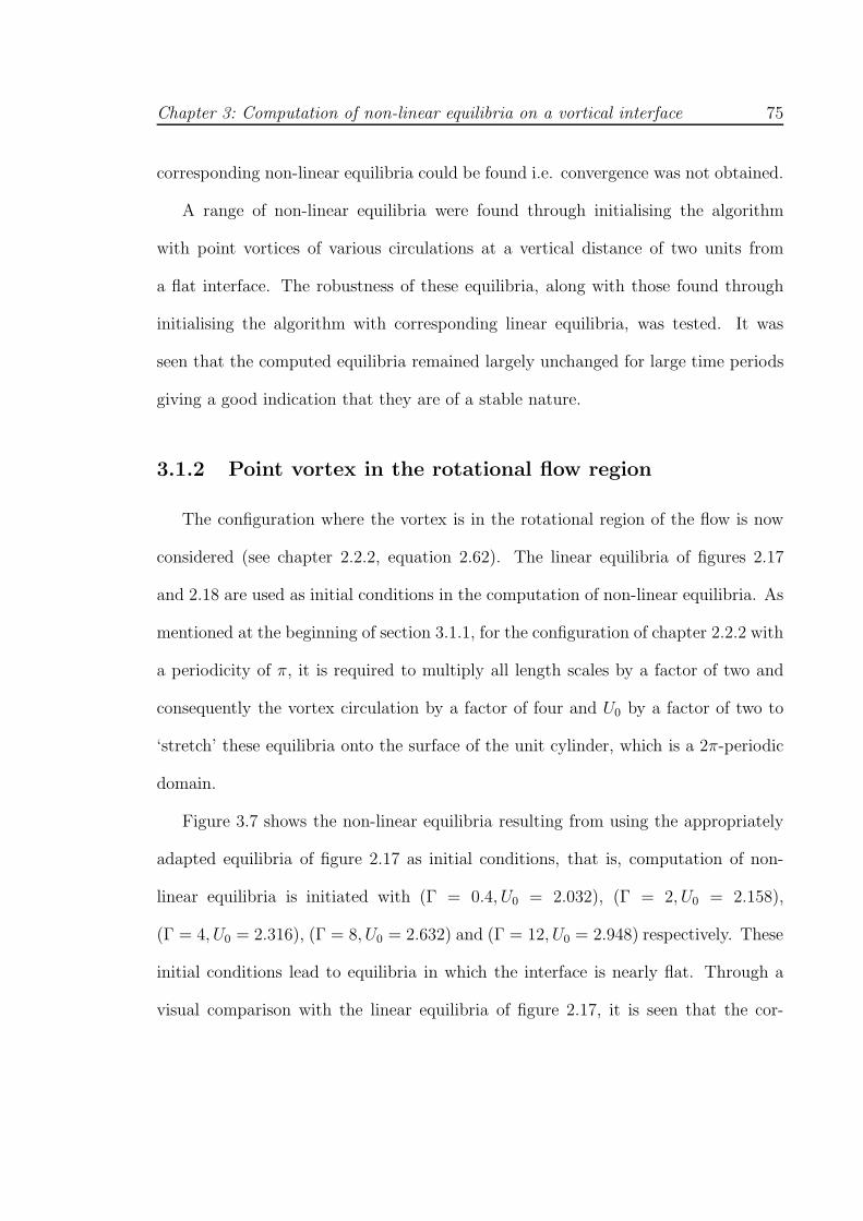
Chapter 3: Computation of non-linear equilibria on a vortical interface 75
corresponding non-linear equilibria could be found i.e. convergence was not obtained.
A range of non-linear equilibria were found through initialising the algorithm
with point vortices of various circulations at a vertical distance of two units from
a flat interface. The robustness of these equilibria, along with those found through
initialising the algorithm with corresponding linear equilibria, was tested. It was
seen that the computed equilibria remained largely unchanged for large time periods
giving a good indication that they are of a stable nature.
3.1.2 Point vortex in the rotational flow region
The configuration where the vortex is in the rotational region of the flow is now
considered (see chapter 2.2.2, equation 2.62). The linear equilibria of figures 2.17
and 2.18 are used as initial conditions in the computation of non-linear equilibria. As
mentioned at the beginning of section 3.1.1, for the configuration of chapter 2.2.2 with
a periodicity of π, it is required to multiply all length scales by a factor of two and
consequently the vortex circulation by a factor of four and U0 by a factor of two to
‘stretch’ these equilibria onto the surface of the unit cylinder, which is a 2π-periodic
domain.
Figure 3.7 shows the non-linear equilibria resulting from using the appropriately
adapted equilibria of figure 2.17 as initial conditions, that is, computation of non-
linear equilibria is initiated with (Γ = 0.4, U0 = 2.032), (Γ = 2, U0 = 2.158),
(Γ = 4, U0 = 2.316), (Γ = 8, U0 = 2.632) and (Γ = 12, U0 = 2.948) respectively. These
initial conditions lead to equilibria in which the interface is nearly flat. Through a
visual comparison with the linear equilibria of figure 2.17, it is seen that the cor-
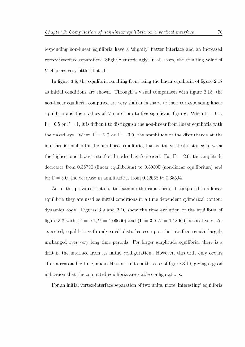
Chapter 3: Computation of non-linear equilibria on a vortical interface 76
responding non-linear equilibria have a ‘slightly’ flatter interface and an increased
vortex-interface separation. Slightly surprisingly, in all cases, the resulting value of
U changes very little, if at all.
In figure 3.8, the equilibria resulting from using the linear equilibria of figure 2.18
as initial conditions are shown. Through a visual comparison with figure 2.18, the
non-linear equilibria computed are very similar in shape to their corresponding linear
equilibria and their values of U match up to five significant figures. When Γ = 0.1,
Γ = 0.5 or Γ = 1, it is difficult to distinguish the non-linear from linear equilibria with
the naked eye. When Γ = 2.0 or Γ = 3.0, the amplitude of the disturbance at the
interface is smaller for the non-linear equilibria, that is, the vertical distance between
the highest and lowest interfacial nodes has decreased. For Γ = 2.0, the amplitude
decreases from 0.38790 (linear equilibrium) to 0.30305 (non-linear equilibrium) and
for Γ = 3.0, the decrease in amplitude is from 0.52668 to 0.35594.
As in the previous section, to examine the robustness of computed non-linear
equilibria they are used as initial conditions in a time dependent cylindrical contour
dynamics code. Figures 3.9 and 3.10 show the time evolution of the equilibria of
figure 3.8 with (Γ = 0.1, U = 1.00600) and (Γ = 3.0, U = 1.18900) respectively. As
expected, equilibria with only small disturbances upon the interface remain largely
unchanged over very long time periods. For larger amplitude equilibria, there is a
drift in the interface from its initial configuration. However, this drift only occurs
after a reasonable time, about 50 time units in the case of figure 3.10, giving a good
indication that the computed equilibria are stable configurations.
For an initial vortex-interface separation of two units, more ‘interesting’ equilibria
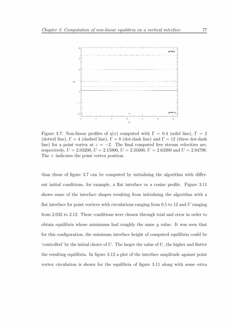
Chapter 3: Computation of non-linear equilibria on a vortical interface 77
Figure 3.7: Non-linear profiles of η(x) computed with Γ = 0.4 (solid line), Γ = 2(dotted line), Γ = 4 (dashed line), Γ = 8 (dot-dash line) and Γ = 12 (three dot-dashline) for a point vortex at z = −2. The final computed free stream velocities are,respectively, U = 2.03200, U = 2.15800, U = 2.31600, U = 2.63200 and U = 2.94798.The + indicates the point vortex position.
than those of figure 3.7 can be computed by initialising the algorithm with differ-
ent initial conditions, for example, a flat interface or a cosine profile. Figure 3.11
shows some of the interface shapes resulting from initialising the algorithm with a
flat interface for point vortices with circulations ranging from 0.5 to 12 and U ranging
from 2.032 to 2.12. These conditions were chosen through trial and error in order to
obtain equilibria whose minimums had roughly the same y value. It was seen that
for this configuration, the minimum interface height of computed equilibria could be
‘controlled’ by the initial choice of U . The larger the value of U , the higher and flatter
the resulting equilibria. In figure 3.12 a plot of the interface amplitude against point
vortex circulation is shown for the equilibria of figure 3.11 along with some extra
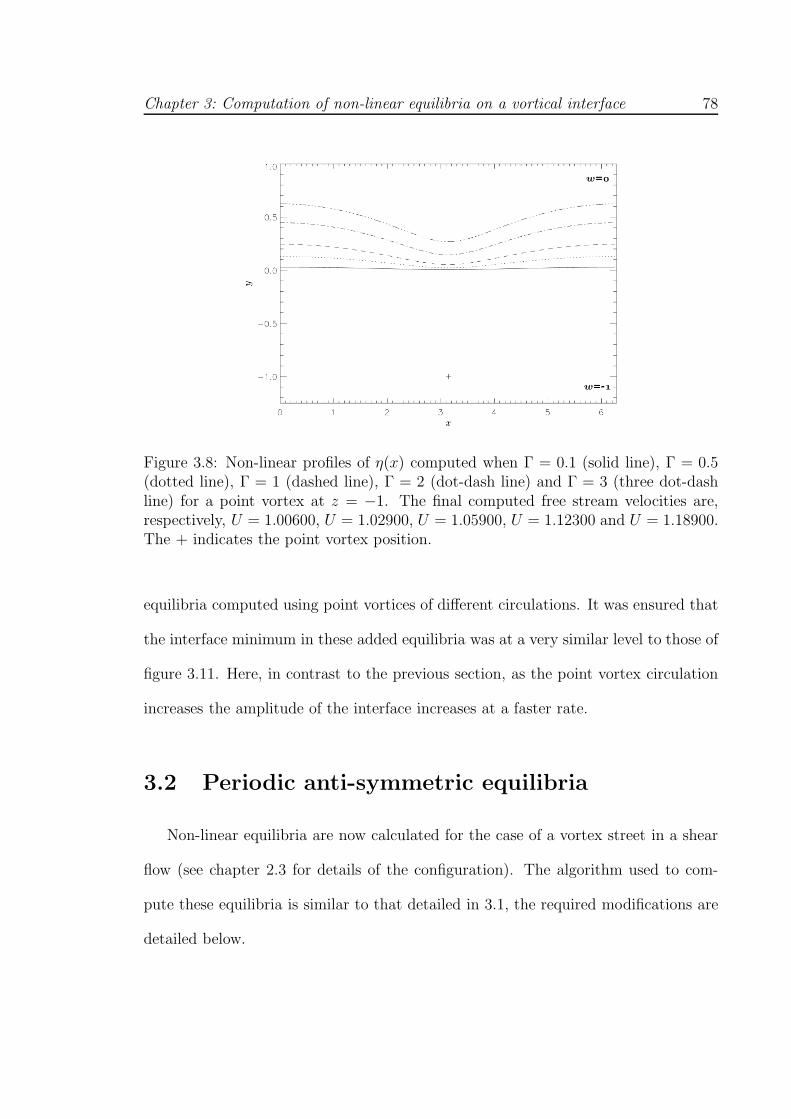
Chapter 3: Computation of non-linear equilibria on a vortical interface 78
Figure 3.8: Non-linear profiles of η(x) computed when Γ = 0.1 (solid line), Γ = 0.5(dotted line), Γ = 1 (dashed line), Γ = 2 (dot-dash line) and Γ = 3 (three dot-dashline) for a point vortex at z = −1. The final computed free stream velocities are,respectively, U = 1.00600, U = 1.02900, U = 1.05900, U = 1.12300 and U = 1.18900.The + indicates the point vortex position.
equilibria computed using point vortices of different circulations. It was ensured that
the interface minimum in these added equilibria was at a very similar level to those of
figure 3.11. Here, in contrast to the previous section, as the point vortex circulation
increases the amplitude of the interface increases at a faster rate.
3.2 Periodic anti-symmetric equilibria
Non-linear equilibria are now calculated for the case of a vortex street in a shear
flow (see chapter 2.3 for details of the configuration). The algorithm used to com-
pute these equilibria is similar to that detailed in 3.1, the required modifications are
detailed below.
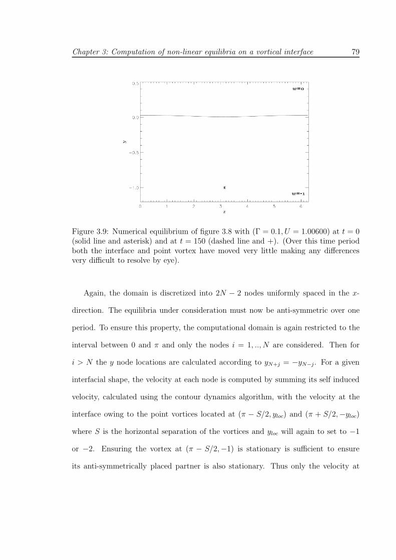
Chapter 3: Computation of non-linear equilibria on a vortical interface 79
Figure 3.9: Numerical equilibrium of figure 3.8 with (Γ = 0.1, U = 1.00600) at t = 0(solid line and asterisk) and at t = 150 (dashed line and +). (Over this time periodboth the interface and point vortex have moved very little making any differencesvery difficult to resolve by eye).
Again, the domain is discretized into 2N − 2 nodes uniformly spaced in the x-
direction. The equilibria under consideration must now be anti-symmetric over one
period. To ensure this property, the computational domain is again restricted to the
interval between 0 and π and only the nodes i = 1, .., N are considered. Then for
i > N the y node locations are calculated according to yN+j = −yN−j. For a given
interfacial shape, the velocity at each node is computed by summing its self induced
velocity, calculated using the contour dynamics algorithm, with the velocity at the
interface owing to the point vortices located at (π − S/2, yloc) and (π + S/2,−yloc)
where S is the horizontal separation of the vortices and yloc will again to set to −1
or −2. Ensuring the vortex at (π − S/2,−1) is stationary is sufficient to ensure
its anti-symmetrically placed partner is also stationary. Thus only the velocity at
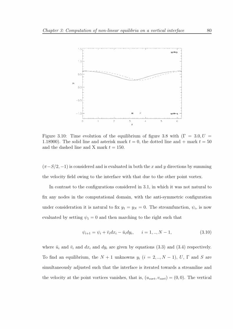
Chapter 3: Computation of non-linear equilibria on a vortical interface 80
Figure 3.10: Time evolution of the equilibrium of figure 3.8 with (Γ = 3.0, U =1.18900). The solid line and asterisk mark t = 0, the dotted line and + mark t = 50and the dashed line and X mark t = 150.
(π−S/2,−1) is considered and is evaluated in both the x and y directions by summing
the velocity field owing to the interface with that due to the other point vortex.
In contrast to the configurations considered in 3.1, in which it was not natural to
fix any nodes in the computational domain, with the anti-symmetric configuration
under consideration it is natural to fix y1 = yN = 0. The streamfunction, ψi, is now
evaluated by setting ψ1 = 0 and then marching to the right such that
ψi+1 = ψi + vidxi − uidyi, i = 1, .., N − 1, (3.10)
where ui and vi and dxi and dyi are given by equations (3.3) and (3.4) respectively.
To find an equilibrium, the N + 1 unknowns yi (i = 2, .., N − 1), U , Γ and S are
simultaneously adjusted such that the interface is iterated towards a streamline and
the velocity at the point vortices vanishes, that is, (uvort, vvort) = (0, 0). The vertical
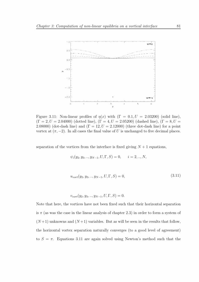
Chapter 3: Computation of non-linear equilibria on a vortical interface 81
Figure 3.11: Non-linear profiles of η(x) with (Γ = 0.1, U = 2.03200) (solid line),(Γ = 2, U = 2.04000) (dotted line), (Γ = 4, U = 2.05200) (dashed line), (Γ = 8, U =2.08000) (dot-dash line) and (Γ = 12, U = 2.12000) (three dot-dash line) for a pointvortex at (π,−2). In all cases the final value of U is unchanged to five decimal places.
separation of the vortices from the interface is fixed giving N + 1 equations,
ψi(y2, y3, .., yN−1, U,Γ, S) = 0, i = 2, .., N,
uvort(y2, y3, .., yN−1, U,Γ, S) = 0,
vvort(y2, y3, .., yN−1, U,Γ, S) = 0.
(3.11)
Note that here, the vortices have not been fixed such that their horizontal separation
is π (as was the case in the linear analysis of chapter 2.3) in order to form a system of
(N+1) unknowns and (N+1) variables. But as will be seen in the results that follow,
the horizontal vortex separation naturally converges (to a good level of agreement)
to S = π. Equations 3.11 are again solved using Newton’s method such that the
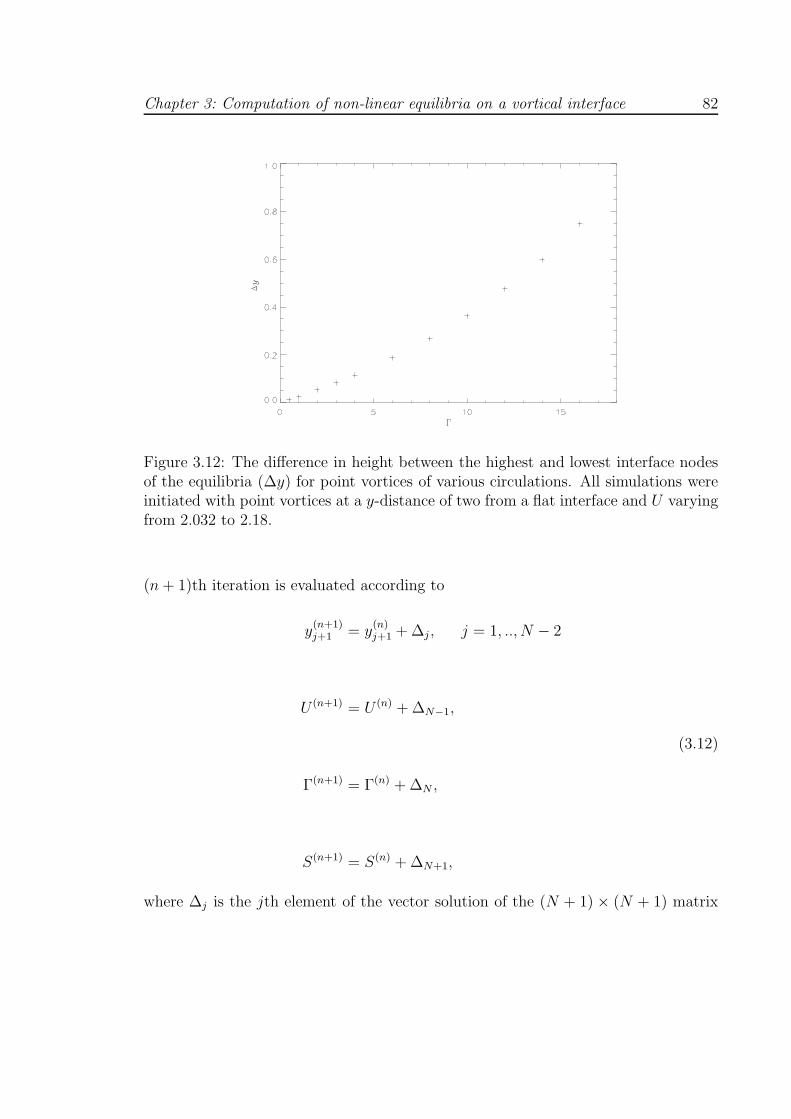
Chapter 3: Computation of non-linear equilibria on a vortical interface 82
Figure 3.12: The difference in height between the highest and lowest interface nodesof the equilibria (∆y) for point vortices of various circulations. All simulations wereinitiated with point vortices at a y-distance of two from a flat interface and U varyingfrom 2.032 to 2.18.
(n+ 1)th iteration is evaluated according to
y(n+1)j+1 = y
(n)j+1 + ∆j , j = 1, .., N − 2
U (n+1) = U (n) + ∆N−1,
Γ(n+1) = Γ(n) + ∆N ,
S(n+1) = S(n) + ∆N+1,
(3.12)
where ∆j is the jth element of the vector solution of the (N + 1) × (N + 1) matrix
Chapter 3: Computation of non-linear equilibria on a vortical interface 83
equation
N−2∑
j=1
∂ψ(n)i+1
∂yj+1∆j +
∂ψ(n)i+1
∂U∆N−1 +
∂ψ(n)i+1
∂Γ∆N +
∂ψ(n)i+1
∂Γ∆S = −ψ(n)
i+1, i = 1, .., N − 1,
N−2∑
j=1
∂u(n)vort
∂yj+1∆j +
∂u(n)vort
∂U∆N−1
∂u(n)vort
∂Γ∆N
∂u(n)vort
∂S∆N+1 = −u(n)
vort,
N−2∑
j=1
∂v(n)vort
∂yj+1∆j +
∂v(n)vort
∂U∆N−1
∂v(n)vort
∂Γ∆N
∂v(n)vort
∂S∆N+1 = −u(n)
vort.
(3.13)
The derivatives in (3.13) are again computed numerically according to (3.9). The
number of nodes in the computational domain is now set to N = 150, giving a
resolution in the x-direction of δx = 0.02094. Increasing the number of nodes within
the computation does not alter the results to the quoted level of accuracy. Typically,
convergence was realised within 50 iterations.
In figure 3.13 the non-linear equilibria resulting from initialising the algorithm
with the linear equilibria of chapter 2.3, figures 2.20 and 2.21 are shown. These
linear equilibria were derived in a π-periodic domain and have thus once again been
‘stretched’ onto the unit cylinder. The initial conditions used in computing these
equilibria were given by (Γ0 = −16, U0 = −0.288, S0 = π), (Γ0 = −8, U0 = 0.280, S0 =
π), (Γ0 = −2, U0 = 0.862, S0 = π), (Γ0 = −1, U0 = 0.930, S0 = π) and (Γ0 =
2, U0 = 1.144, S0 = π), where the circulation given is that of the vortex in the region
x ∈ [0, 2π) and the 0 subscript indicates the initial value of the parameter in question.
In all computations the vortex circulation remained unchanged to 5 decimal places, as
Chapter 3: Computation of non-linear equilibria on a vortical interface 84
did the horizontal vortex separation parameter S. (It should be noted that increasing
the x-direction resolution resulted in Γ and S remaining unchanged to five decimal
places. In the following text, for the sake of brevity, the given value of Γ will be
accurate to five decimal places, i.e. Γ = 1 means Γ = 1.00000).
For the vortices with Γ = −16 and Γ = −8 the interface was initially curved
towards them (see figure 2.22). However, in the non-linear equilibria resulting from
these initial configurations, the interface has ‘reversed’ and is now curved away from
the point vortices (figure 3.13). The non-linear equilibria with Γ = −2 and Γ = −1 are
similar in shape but have a lower amplitude in comparison to their linear counterparts
of figure 2.21. The non-linear equilibria for Γ = −16 and Γ = −8 are thus similar in
shape to the equilibria with Γ = −2 and Γ = −1 but have larger amplitudes owing
to the larger circulations of the point vortices involved. Conversely, when Γ = 2, the
resulting non-linear equilibria is of a similar shape but has a greater amplitude than
its linear counterpart, compare figures 2.21 (linear equilibria) and 3.13 (non-linear
equilibria).
Figure 3.14 shows the non-linear equilibria resulting from initialising the algorithm
with the linear equilibria of figure 2.25, thus, the initial conditions are given by
(Γ0 = −1, U0 = 0.620, S0 = π) and (Γ0 = −0.1, U0 = 0.544, S0 = π). In both
cases, the vortex circulation and separation parameter S again remain unchanged
to 5 decimal places and the final free stream velocities are slightly lower than their
initialisation values. Through a visual comparison with the initial interface shapes
shown in figure 2.25 it is seen that the non-linear shapes are very similar. It is worth
noting that when the algorithm was initialised with the linear equilibria of figure 2.24,
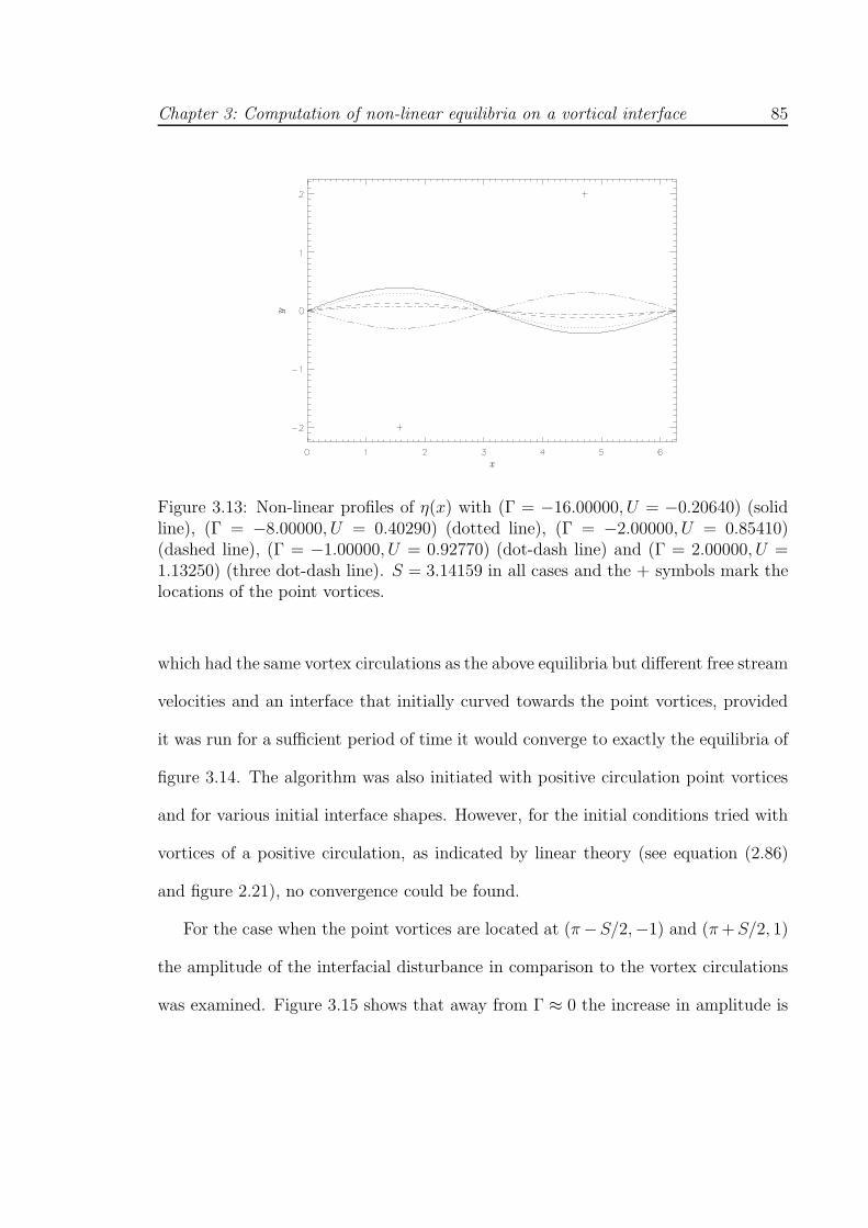
Chapter 3: Computation of non-linear equilibria on a vortical interface 85
Figure 3.13: Non-linear profiles of η(x) with (Γ = −16.00000, U = −0.20640) (solidline), (Γ = −8.00000, U = 0.40290) (dotted line), (Γ = −2.00000, U = 0.85410)(dashed line), (Γ = −1.00000, U = 0.92770) (dot-dash line) and (Γ = 2.00000, U =1.13250) (three dot-dash line). S = 3.14159 in all cases and the + symbols mark thelocations of the point vortices.
which had the same vortex circulations as the above equilibria but different free stream
velocities and an interface that initially curved towards the point vortices, provided
it was run for a sufficient period of time it would converge to exactly the equilibria of
figure 3.14. The algorithm was also initiated with positive circulation point vortices
and for various initial interface shapes. However, for the initial conditions tried with
vortices of a positive circulation, as indicated by linear theory (see equation (2.86)
and figure 2.21), no convergence could be found.
For the case when the point vortices are located at (π−S/2,−1) and (π+S/2, 1)
the amplitude of the interfacial disturbance in comparison to the vortex circulations
was examined. Figure 3.15 shows that away from Γ ≈ 0 the increase in amplitude is
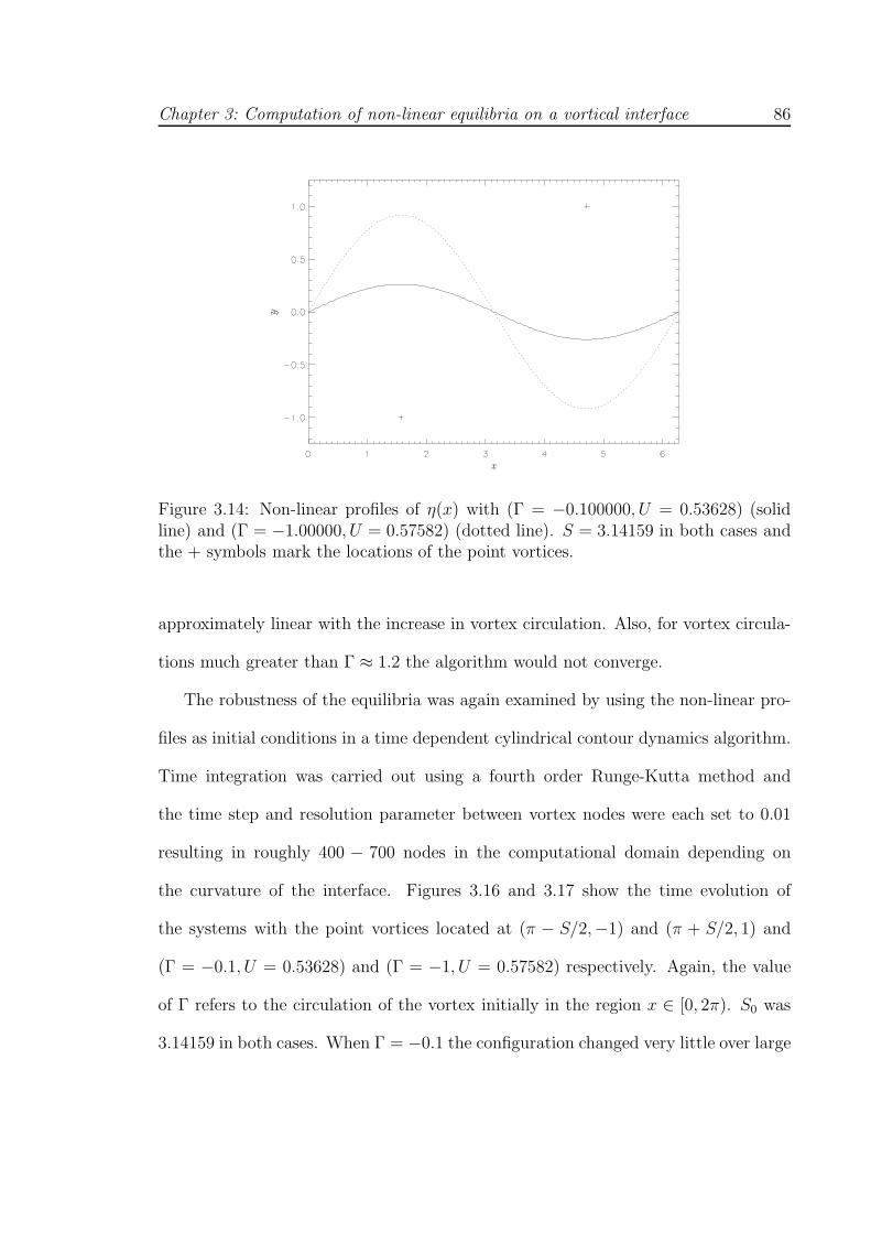
Chapter 3: Computation of non-linear equilibria on a vortical interface 86
Figure 3.14: Non-linear profiles of η(x) with (Γ = −0.100000, U = 0.53628) (solidline) and (Γ = −1.00000, U = 0.57582) (dotted line). S = 3.14159 in both cases andthe + symbols mark the locations of the point vortices.
approximately linear with the increase in vortex circulation. Also, for vortex circula-
tions much greater than Γ ≈ 1.2 the algorithm would not converge.
The robustness of the equilibria was again examined by using the non-linear pro-
files as initial conditions in a time dependent cylindrical contour dynamics algorithm.
Time integration was carried out using a fourth order Runge-Kutta method and
the time step and resolution parameter between vortex nodes were each set to 0.01
resulting in roughly 400 − 700 nodes in the computational domain depending on
the curvature of the interface. Figures 3.16 and 3.17 show the time evolution of
the systems with the point vortices located at (π − S/2,−1) and (π + S/2, 1) and
(Γ = −0.1, U = 0.53628) and (Γ = −1, U = 0.57582) respectively. Again, the value
of Γ refers to the circulation of the vortex initially in the region x ∈ [0, 2π). S0 was
3.14159 in both cases. When Γ = −0.1 the configuration changed very little over large
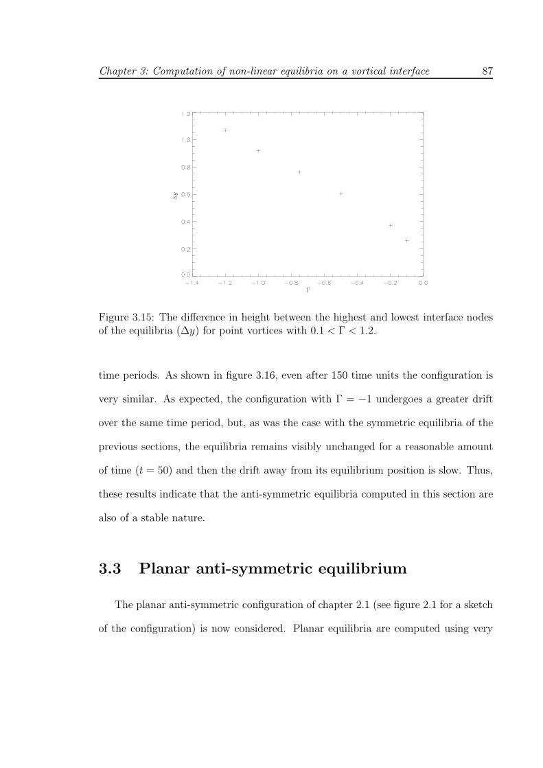
Chapter 3: Computation of non-linear equilibria on a vortical interface 87
Figure 3.15: The difference in height between the highest and lowest interface nodesof the equilibria (∆y) for point vortices with 0.1 < Γ < 1.2.
time periods. As shown in figure 3.16, even after 150 time units the configuration is
very similar. As expected, the configuration with Γ = −1 undergoes a greater drift
over the same time period, but, as was the case with the symmetric equilibria of the
previous sections, the equilibria remains visibly unchanged for a reasonable amount
of time (t = 50) and then the drift away from its equilibrium position is slow. Thus,
these results indicate that the anti-symmetric equilibria computed in this section are
also of a stable nature.
3.3 Planar anti-symmetric equilibrium
The planar anti-symmetric configuration of chapter 2.1 (see figure 2.1 for a sketch
of the configuration) is now considered. Planar equilibria are computed using very
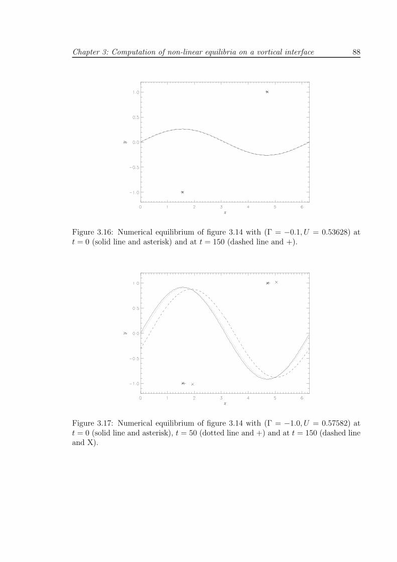
Chapter 3: Computation of non-linear equilibria on a vortical interface 88
Figure 3.16: Numerical equilibrium of figure 3.14 with (Γ = −0.1, U = 0.53628) att = 0 (solid line and asterisk) and at t = 150 (dashed line and +).
Figure 3.17: Numerical equilibrium of figure 3.14 with (Γ = −1.0, U = 0.57582) att = 0 (solid line and asterisk), t = 50 (dotted line and +) and at t = 150 (dashed lineand X).
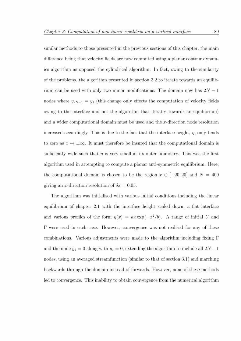
Chapter 3: Computation of non-linear equilibria on a vortical interface 89
similar methods to those presented in the previous sections of this chapter, the main
difference being that velocity fields are now computed using a planar contour dynam-
ics algorithm as opposed the cylindrical algorithm. In fact, owing to the similarity
of the problems, the algorithm presented in section 3.2 to iterate towards an equilib-
rium can be used with only two minor modifications: The domain now has 2N − 1
nodes where y2N−1 = y1 (this change only effects the computation of velocity fields
owing to the interface and not the algorithm that iterates towards an equilibrium)
and a wider computational domain must be used and the x-direction node resolution
increased accordingly. This is due to the fact that the interface height, η, only tends
to zero as x → ±∞. It must therefore be insured that the computational domain is
sufficiently wide such that η is very small at its outer boundary. This was the first
algorithm used in attempting to compute a planar anti-symmetric equilibrium. Here,
the computational domain is chosen to be the region x ∈ [−20, 20] and N = 400
giving an x-direction resolution of δx = 0.05.
The algorithm was initialised with various initial conditions including the linear
equilibrium of chapter 2.1 with the interface height scaled down, a flat interface
and various profiles of the form η(x) = ax exp(−x2/b). A range of initial U and
Γ were used in each case. However, convergence was not realised for any of these
combinations. Various adjustments were made to the algorithm including fixing Γ
and the node y2 = 0 along with y1 = 0, extending the algorithm to include all 2N −1
nodes, using an averaged streamfunction (similar to that of section 3.1) and marching
backwards through the domain instead of forwards. However, none of these methods
led to convergence. This inability to obtain convergence from the numerical algorithm
Chapter 3: Computation of non-linear equilibria on a vortical interface 90
along with the null result from linear theory (chapter 2.1) gives a good indication that
no such equilibrium exists.
3.4 Summary
Corresponding non-linear equilibria have been computed for the periodic configu-
rations considered in chapter 2, namely, a row of symmetrically placed vortices near
a vorticity interface and a vortex street in a shear flow. For the symmetric config-
uration, the problem was considered for both when the vortices lie in the rotational
and irrotational region of the flow. Periodicity was accounted for by considering the
problem on the surface of the unit cylinder, where the cylinder represents one period
of the configuration. For the planar anti-symmetric configuration (chapter 2.1), as
with linear theory, no equilibrium state could be found.
Symmetric equilibria in which the vortex lies in the irrotational region of flow have
similar characteristics to some of the small amplitude linear equilibria in that, the
hump on the interface lies symmetrically above the vortex. As the vortex circulation
increases, equilibria have larger amplitude disturbances on the interface or alterna-
tively, there is a larger vortex-interface separation. Which of these states is achieved
is dependent on the choice of initial conditions. Equilibria in which the interface lies
within unit distance of the point vortex, or in which higher order modes are present,
could not be found. Computed equilibria were proven to be robust by using them as
initial conditions in a time dependent code with, only small drifts from equilibrium
positions were observed over long time periods.
When the vortex lies in the rotational region of the flow, linear theory again proves
Chapter 3: Computation of non-linear equilibria on a vortical interface 91
to be a good guide as to what shapes can be computed. In these equilibria, the
hump on the interface was now placed anti-symmetrically above the vortex. Again,
for a specific value of Γ, many equilibria could be computed. Equilibria with larger
amplitude oscillations at the interface tend to have a lower vortex-interface separation
along with a lower free stream velocity. Faster free stream velocities lead to a flatter
interface shapes with a greater vortex-interface separation. The equilibria were again
shown to be robust giving a good indication of their stability.
For the vortex street configuration, interface shapes were found in which the inter-
face curved towards the vortices when Γ > 0 and away from them when Γ < 0 (here
Γ refers to the circulation of the vortex in the region x ∈ [0, π]). However, when the
vortices were placed at unit distance from the interface, only equilibria with Γ < 0
could be found. Equilibria were again used as initial conditions in a time dependent
code and again only underwent small deviations over long periods of time giving a
good indication that they are stable. It is hoped that the equilibria computed here
may be of help in explaining the longevity of some vortical configurations observed
in planetary atmospheres and oceans.
Chapter 4
Vortex-wave interaction on the
surface of a sphere
Strong zonal shear flows are frequently observed in the Earth’s atmosphere and
ocean and also on the giant planets. Such shear flows are able to support wave
motion and it is of interest to understand how small, intense vortices interact with
these flows. One area of such interactions in the Earth’s atmosphere is the Gulf
stream. Meanders of the Gulf stream can sometimes detach and form cyclonic or
anti-cyclonic structures. The resulting interaction between these detached eddies and
the Gulf stream play an important role in water vapour mixing across the Atlantic
region and hence in the weather patterns seen across much of Western Europe. With
this region in mind, Stern and Flierl (1987) consider the interaction between a point
vortex and shear flows on the f -plane in which two regions of constant vorticity
owing to the shear flow are separated by a single interface. Results showed that an
anticyclonic vortex located in the region of high vorticity generated a perturbation
92
Chapter 4: Vortex-wave interaction on the surface of a sphere 93
upon the interface resulting in a “westward” propagation. Results also demonstrated
that when the vortex was located sufficiently close to the interface, the vortex would
cause the interface to wrap around it. Bell (1990) considers time-dependent vortex-
wave interaction in flows with piecewise constant vorticity of the type considered in
chapter 2 and 3. He shows that for a vortex-wave interaction in a planar shear flow,
a positive (cyclonic) vortex drifts in the direction of increasing potential vorticity by
radiating interfacial waves, while a negative (anti-cyclonic) vortex will drift towards
regions of lower vorticity. Then, with applications to transport and mixing between
rotational and irrotational flows, Atassi (1998) considers the problem of point vortex
interaction with a wall-bounded shear layer. The study showed that the interaction
between the point vortex and shear layer is strongest when the vortex and layer are of
opposite signed vorticity. Strong interactions resulted in the ejection of fluid from the
shear layer and such ejections were associated with a significant rise in the magnitude
of wall pressure.
Much research has been conducted into the interaction of point vortices with to-
pography that give rise to a background potential vorticity distribution (see appendix
B). Near continental margins where sharp variations in depth occur, such as the Gulf
of Mexico, to leading order local variations in potential vorticity are dominated by
sharp topographic gradients and it is of interest to examine how such variations in
depth effect the motion of eddies. McDonald (1998) considers the motion of an intense
point vortex near an infinite escarpment in the plane. Intense in this context means
that the vortex circulation time is much shorter than the time scale associated with
wave propagation. Owing to the conservation of potential vorticity, at small times,
Chapter 4: Vortex-wave interaction on the surface of a sphere 94
an intense cyclone’s motion is towards regions of lower potential vorticity whilst an
anticyclones motion is in the opposite direction. Following this initial motion, a
steady motion parallel to the escarpment ensues before the vortex resonates with the
topographic wave field resulting in cyclones drifting slowly towards regions of higher
ambient potential vorticity and anticyclones drifting slowly away from such regions.
The remaining cases of moderate and weak point vortices are considered in Dunn
et al. (2001). White and McDonald (2004) then consider the analogous two-layer
fluid problem. The two-layer stratification is chosen such that the height of topog-
raphy in the upper layer is a small fraction of the overall depth enabling the use of
quasi-geostrophic theory which implies that in the upper layer the vorticity is, again,
piecewise constant. Weak vortices in the lower-fluid layer propagate mainly due to
their image in the topography whilst upper-layer vortices propagate much slower and
produce comparatively small amplitude topographic waves. In Newton and Sakajo
(2007) the interaction of a ring of point vortices with a background vorticity initially
in solid body rotation is considered.
The present chapter considers the time dependent problem of a point vortex on
the surface of the non-rotating unit sphere with a background distribution of vorticity
consisting of two opposite signed caps. Unlike previous work conducted in the plane,
on the sphere there is periodicity in the zonal direction. Also, as mentioned in the
beginning to chapter 2, the curvature of the sphere introduces a shielding effect.
The point vortex forcing induces waves upon the vorticity interface which, in turn,
perturb the zonally symmetric flow. The resultant coupled motion of the point vortex
and waves is investigated. Analytic results valid for linear interfacial waves are first
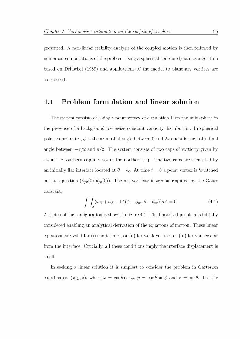
Chapter 4: Vortex-wave interaction on the surface of a sphere 95
presented. A non-linear stability analysis of the coupled motion is then followed by
numerical computations of the problem using a spherical contour dynamics algorithm
based on Dritschel (1989) and applications of the model to planetary vortices are
considered.
4.1 Problem formulation and linear solution
The system consists of a single point vortex of circulation Γ on the unit sphere in
the presence of a background piecewise constant vorticity distribution. In spherical
polar co-ordinates, φ is the azimuthal angle between 0 and 2π and θ is the latitudinal
angle between −π/2 and π/2. The system consists of two caps of vorticity given by
ωS in the southern cap and ωN in the northern cap. The two caps are separated by
an initially flat interface located at θ = θ0. At time t = 0 a point vortex is ‘switched
on’ at a position (φpv(0), θpv(0)). The net vorticity is zero as required by the Gauss
constant,∫ ∫
S
(ωN + ωS + Γδ(φ− φpv, θ − θpv))dA = 0. (4.1)
A sketch of the configuration is shown in figure 4.1. The linearised problem is initially
considered enabling an analytical derivation of the equations of motion. These linear
equations are valid for (i) short times, or (ii) for weak vortices or (iii) for vortices far
from the interface. Crucially, all these conditions imply the interface displacement is
small.
In seeking a linear solution it is simplest to consider the problem in Cartesian
coordinates, (x, y, z), where x = cos θ cosφ, y = cos θ sinφ and z = sin θ. Let the
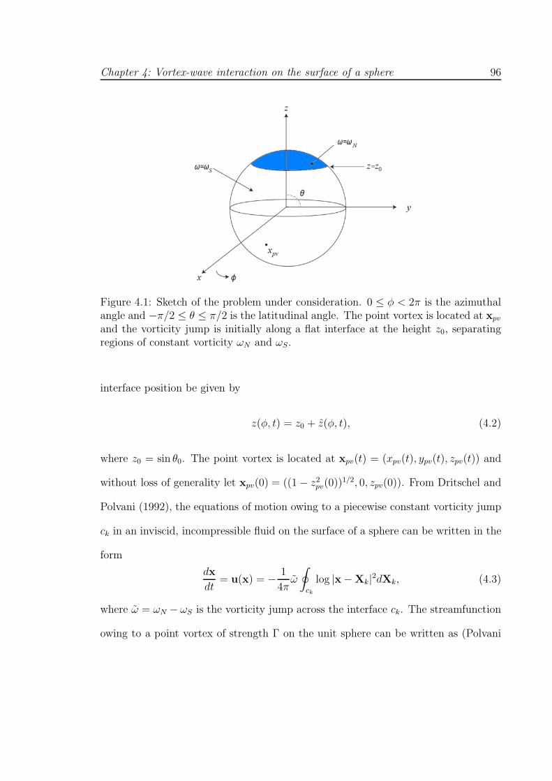
Chapter 4: Vortex-wave interaction on the surface of a sphere 96
Figure 4.1: Sketch of the problem under consideration. 0 ≤ φ < 2π is the azimuthalangle and −π/2 ≤ θ ≤ π/2 is the latitudinal angle. The point vortex is located at xpv
and the vorticity jump is initially along a flat interface at the height z0, separatingregions of constant vorticity ωN and ωS.
interface position be given by
z(φ, t) = z0 + z(φ, t), (4.2)
where z0 = sin θ0. The point vortex is located at xpv(t) = (xpv(t), ypv(t), zpv(t)) and
without loss of generality let xpv(0) = ((1 − z2pv(0))1/2, 0, zpv(0)). From Dritschel and
Polvani (1992), the equations of motion owing to a piecewise constant vorticity jump
ck in an inviscid, incompressible fluid on the surface of a sphere can be written in the
form
dx
dt= u(x) = − 1
4πω
∮
ck
log |x − Xk|2dXk, (4.3)
where ω = ωN − ωS is the vorticity jump across the interface ck. The streamfunction
owing to a point vortex of strength Γ on the unit sphere can be written as (Polvani
Chapter 4: Vortex-wave interaction on the surface of a sphere 97
and Dritschel 1993)
ψ =Γ
4πlog(1 − x · xpv). (4.4)
Note that the global circulation owing to (4.4) is zero, since it includes a uniform
background vorticity of −Γ/4π. The azimuthal and vertical velocities owing to the
point vortex are then retrieved via
dφ
dt= −∂ψ
∂zand
dz
dt=∂ψ
∂φ. (4.5)
To solve the linear vortex-wave interaction problem, the perturbation at the interface,
z(φ, t), is written as a time dependent Fourier series
z(φ, t) = z0 +∞∑
n=1
(an(t) cos(nφ) + bn(t) sin(nφ)) . (4.6)
First, z-direction perturbations at the interface are considered. Substituting (4.6)
into (4.3) gives the self induced vertical velocity of the vorticity jump on the contour.
The total vertical velocity at the contour is given by summing this with the vertical
velocity field due to the point vortex:
dz
dt=∂z
∂t+ Ω0
∂z
∂φ= − ω
4π
∫ 2π
0
log |x(φ, t) − X(α, t)|2 ∂z∂φ
∣
∣
∣
∣
α
dα
+∂
∂φ
Γ
4πlog(1 − x0 · xpv),
(4.7)
where, consistent with linear theory, Ω0 = ω/2 is the angular velocity at an unper-
turbed interface (Dritschel and Polvani 1992). Evaluating and linearising the terms
in (4.7) gives
|x(φ, t) − X(α, t)|2 = 2 cos2 θ0(t)(1 − cos(α− φ)),
x0 · xpv = (1 − z2pv)
12 (1 − z2
0)12 cos(φ− φpv) + zpvz0.
(4.8)
Chapter 4: Vortex-wave interaction on the surface of a sphere 98
Substitution of (4.6) and (4.8) into (4.7) gives
∞∑
n=1
(
an cosnφ+ bn sin nφ+ nω
2(−an sin nφ+ bn cosnφ)
)
=
− ω
4π
∫ 2π
0
log |1 − cos(α− φ)|(
∞∑
n=1
n (−an sin nα + bn cosnα))
)
dα
+Γ
4π
[
(1 − z2pv)
12 (1 − z2
0)12 sin(φ− φpv)
1 − (1 − z2pv)
12 (1 − z2
0)12 cos(φ− φpv) − zpvz0
]
.
(4.9)
Evaluation of the integrals in (4.9) yield the following results:
∫ 2π
0
log |1 − cos(α− φ)|(
∞∑
n=1
(−nan) sinnα)
)
dα = 2π
∞∑
n=0
an sinnφ,
∫ 2π
0
log |1 − cos(α− φ)|(
∞∑
n=1
nbn sin nα
)
dα = −2π
∞∑
n=0
bn cosnφ.
(4.10)
Substituting the integrals (4.10) back into (4.9) gives
∞∑
n=1
[(
an +ω
2(n− 1)bn
)
cosnφ +
(
bn − ω
2(n− 1)an
)
sin nφ
]
=Γ
4π
[
(1 − z2pv)
12 (1 − z2
0)12 sin(φ− φpv)
1 − (1 − z2pv)
12 (1 − z2
0)12 cos(φ− φpv) − zpvz0
]
=Γ
4πF (φ, t).
(4.11)
The RHS forcing term of (4.11) is now written as a Fourier series such that
F (φ, t) =∞∑
n=1
(cn(t) cosnφ+ dn(t) sin nφ) , (4.12)
Chapter 4: Vortex-wave interaction on the surface of a sphere 99
where
cn(t) =1
π
∫ 2π
0
F (φ, t) cosnφdφ
=1
π
∫ 2π
0
(1 − z2pv)
12 (1 − z2
0)12 sin(φ− φpv)
1 − (1 − z2pv)
12 (1 − z2
0)12 cos(φ− φpv) − zpvz0
cosnφdφ,
(4.13)
and
dn(t) =1
π
∫ 2π
0
F (φ, t) sinnφdφ
=1
π
∫ 2π
0
(1 − z2pv)
12 (1 − z2
0)12 sin(φ− φpv)
1 − (1 − z2pv)
12 (1 − z2
0)12 cos(φ− φpv) − zpvz0
sinnφdφ.
(4.14)
Gradshteyn and Ryzhik (1965) give an identity to evaluate integrals of the form seen
in (4.13) and (4.14) which can be written as (Dritschel and Polvani 1992)
−m
2π
∫ 2π
0
log(1−zazb−(1−z2a)
12 (1−z2
b )12 cosβ)eimβdβ =
(
1 − z>
1 + z>
1 + z<
1 − z<
)m/2
, (4.15)
where z> stands for the maximum of za and zb and z< for the minimum. For the case
when z0 > zpv, i.e. when the point vortex is located in the southern cap of vorticity,
the integrals of (4.13) and (4.14) give
cn(t) = −2 sin(nφpv)
(
1 − z01 + z0
1 + zpv
1 − zpv
)n/2
,
dn(t) = 2 cos(nφpv)
(
1 − z01 + z0
1 + zpv
1 − zpv
)n/2
,
(4.16)
where φpv is a function of time determined by integrating the angular velocity of the
point vortex in the azimuthal direction owing to the background vorticity distribution.
This angular velocity is derived below. When z0 > zpv, from (4.15) it is seen that cn(t)
Chapter 4: Vortex-wave interaction on the surface of a sphere 100
and dn(t) will be given by swapping z0s with the zpvs in equations (4.16). To obtain
a coupled set of equations relating the time dependent Fourier coefficients an(t) and
bn(t), (4.16) are substituted into (4.11) giving
an(t) +ω
2(n− 1)bn(t) =
Γ
4πcn(t),
bn(t) − ω
2(n− 1)an(t) =
Γ
4πdn(t),
(4.17)
where n ∈ Z+. An immediate consequence of (4.17) is the impossibility of a steady
solution provided z0 6= ±1 i.e. the vortex is not at a pole. In particular, putting
n = 1 in (4.17) implies that a1 and b1 cannot both be simultaneously zero implying
unsteady behaviour for all time. This of course does not preclude the existence of
non-linear steady solutions.
An infinite set of coupled ordinary differential equations for coefficients an(t) and
bn(t), n = 1, 2, 3, . . . has now been derived. In order to close the linear system, the
equations motion for the point vortex, zpv and φpv are now derived. An approximate
solution can then be obtained by truncating at n = N and solving an 2N +2 coupled
system of ODEs to give the resulting dynamics of the interface and point vortex.
First, an equation for the azimuthal velocity, upv, at the point vortex is sought.
The angular velocity is then given by
φ = upv/(1 − z2pv)
1/2. (4.18)
Using (4.3), the azimuthal velocity at the point vortex is given by
upv = − ω
4π
∮
log |xpv −X(α)|2 ∂∂α
[
(1 − z2(α))12 sinα
]
dα. (4.19)
Chapter 4: Vortex-wave interaction on the surface of a sphere 101
Expanding and linearising the log term of (4.19) gives
|xpv − X(α)|2 = 2(1 − z0zpv − (1 − z20)
12 (1 − z2
pv)12 cos(α− φpv)), (4.20)
and therefore
upv = − ω
4π
∫ 2π
0
log |1 − z0zpv − (1 − z20)
12 (1 − z2
pv)12 cos(α− φpv)|
× ∂
∂α
[
(1 − z2(α))12 sinα
]
dα
= − ω
4π
∫ 2π
0
log |1 − z0zpv − (1 − z20)
12 (1 − z2
pv)12 cos(α− φpv)|
×(
(1 − z20)
12 cosα− z0zα sinα
(1 − z20)
12
)
dα,
(4.21)
where z =∑∞
n=1(an(t) cosnα+bn(t) sinnα) (see (4.6)). Equation (4.21) represents the
flow due to an unperturbed interface plus a small modification due to perturbations
at the interface induced by the point vortex, that is
upv = u0 + u′pv, (4.22)
where (Polvani and Dritschel 1993)
u0 = − ω
4π
∫ 2π
0
log |1 − z0zpv − (1 − z20)
12 (1 − z2
pv)12 cos(α− φpv)|(1 − z2
0)12 cosαdα
=ω
2(1 − z0)
(
1 + zpv
1 − zpv
)12
,
(4.23)
Chapter 4: Vortex-wave interaction on the surface of a sphere 102
and
u′pv = − ω
4π
∫ 2π
0
log |1 − z0zpv − (1 − z20)
12 (1 − z2
pv)12 cos(α− φpv)|
× −z0 sinα
(1 − z20)
12
(−nan sin nα + nbn cosnα)dα
=ωz0
4π(1 − z20)
12
∫ 2π
0
log |1 − z0zpv − (1 − z20)
12 (1 − z2
pv)12 cos(α− φpv)|
× sinα(−nan sin nα + nbn cosnα)dα.
(4.24)
To evaluate the integral in (4.24) the substitution β = α − φpv in made and use is
made of the following trigonometric identities
sinα sin β =1
2(cos(α− β) − cos(α + β)), (4.25)
and
sinα cosβ =1
2(sin(α− β) + sin(α + β)). (4.26)
This yields
u′pv =∞∑
n=1
nωz0
4(1 − z20)
12
[
1
n− 1
(
1 − z01 + z0
1 + zpv
1 − zpv
)n−1
2
(an cos(n− 1)φpv − bn sin(n− 1)φpv)−
(
1 − z01 + z0
1 + zpv
1 − zpv
)n+1
2
(an + bnn+ 1) cos(n+ 1)φpv
]
.
(4.27)
An equation for u′pv has now been derived. However, (4.27) is not valid for n = 1
and therefore, this is considered as a special case. Substituting n = 1 into (4.24) and
Chapter 4: Vortex-wave interaction on the surface of a sphere 103
again using the substitution β = α− φpv gives
u′pv =ωz0
8π(1 − z20)
12
∫ 2π
0
log |1 − z0zpv − (1 − z20)
12 (1 − z2
pv)12 cosβ|
× (a1(cos 2φpv cos 2β − 1) + b1 sin 2φpv cos 2β)dβ
= − ωz0
8(1 − z20)
12
[
(a1 cos 2φpv + b1 sin 2φpv)
(
1 − z01 + z0
1 + zpv
1 − zpv
)
+ a1
(
log[1 − z0zpv] + log
[
1 + (1 −R2)12
2
])]
(4.28)
where R = (1 − z20)
1/2(1 − z2pv)
1/2/(1 − z0zpv). Equations (4.18), (4.23), (4.27) and
(4.28) give finally
φpv = − ωs
(1 − z2pv)
12
(
1 + zpv
1 − zpv
)12
− ωz0
8(1 − z20)
12 (1 − z2
pv)12
×[
(a1 cos 2φpv + b1 sin 2φpv)A+ a1 log
[
(1 − z0zpv)1 + (1 − R2)
12
2
]]
+∞∑
n=2
nωz0
4(1 − z20)
12 (1 − z2
pv)12
[
1
n− 1A
n−12 (an cos(n− 1)φpv − bn sin(n− 1)φpv)
− An+1
2
(
an + bnn+ 1
)
cos(n + 1)φpv
]
.
(4.29)
where, consistent with linear theory, A =(
1−z0
1+z0
1+zpv(0)1−zpv(0)
)
is a constant. Now, from
Chapter 4: Vortex-wave interaction on the surface of a sphere 104
(4.3) the point vortex velocity in the z-direction is given by
zpv = − ω
4π
∫ 2π
0
log |xpv −X(α)|2 ∂z∂α
dα. (4.30)
Substituting in the expression for z given in (4.6) gives
zpv = − ω
4π
∫ 2π
0
log |xpv − X(α)|2∞∑
n=1
(−nan sinnα + nbn cos nα)dα. (4.31)
Expanding and linearising |xpv − X(α)|2, and then integrating gives
zpv = −∞∑
n=1
ω
2A
n2 (an sinnφpv − bn cosnφpv). (4.32)
Truncating the sums in (4.29) and (4.32) at n = N gives a system of 2N + 2 ODEs
for the 2N + 2 unknowns a1, .., aN , b1, .., bN , φpv and zpv governing the motion of a
point vortex located below a vorticity interface on the surface of the sphere in the
limit of small amplitude waves upon the interface. In the following sections, the short
time behaviour of the system and the effect of truncating the system at n = 1 will
be examined. Following this, the linear system will be truncated at higher n and the
resulting motion examined.
Chapter 4: Vortex-wave interaction on the surface of a sphere 105
4.2 Short time behaviour and the n = 1 system
Initially, only the primary mode will be considered. Truncating (4.16), (4.17),
(4.29) and (4.32) at n = 1 gives the following system of ODEs
a1(t) = − Γ
2πA
12 sin φpv,
b1(t) =Γ
2πA
12 cosφpv,
φpv(t) = − ωs
(1 − z2pv)
12
(
1 + zpv
1 − zpv
)12
− ωz0
8(1 − z20)
12 (1 − z2
pv)12
[
(a1 cos 2φpv + b1 sin 2φpv)A
+ a1 log
[
(1 − z0zpv)1 + (1 −R2)
12
2
]]
,
zpv(t) = − ω
2A
12 (a1 sinφpv − b1 cos φpv),
(4.33)
with initial conditions a1(0) = b1(0) = 0, φpv(0) = 0 and 0 ≤ zpv(0) ≤ 1.
Before considering the full n = 1 system, it is insightful to make further relevant
approximations to examine the initial movements of the system. When t is close
to zero it is reasonable to assume that the azimuthal velocity of the point vortex is
constant (i.e. its velocity is that due to an unperturbed interface). This is the velocity
given in (4.23). Taking the southern cap to be of negative vorticity and northern cap
to be of positive vorticity, an eastward azimuthal velocity will be induced at the
vortex. (A westward zonal velocity is induced in the case where the vorticity of the
Chapter 4: Vortex-wave interaction on the surface of a sphere 106
caps is reversed). Therefore, for small times, the azimuthal position of the vortex is
approximately
φpv = Ω0t, (4.34)
where Ω0 is given by (4.23) and (4.18). The Fourier coefficients a1 and b1 can now be
integrated to give
a1(t) =ΓA1/2
Ω0cos Ω0t−
ΓA1/2
Ω0,
b1(t) =ΓA1/2
Ω0sin Ω0t,
(4.35)
and therefore from (4.33)
zpv =ωAΓ
2Ω0
sin Ω0t. (4.36)
For t << Ω−10 (4.36) gives
zpv ≈ ωAΓt
2. (4.37)
Equation (4.37) shows that sgn(zpv) = sgn(ωΓ) (where ω = ωN − ωS is the vorticity
jump across the interface) and thus a point vortex in a region of same-signed vor-
ticity will initially move away from the interface, whilst a point vortex in a region
of opposite-signed vorticity will initially move towards it. While this analysis has
been carried out assuming zpv < z0, the same conclusion holds for zpv > z0. The
required modifications for this case are the substitution of A =(
1+z0
1−z0
1−zpv
1+zpv
)
for A
and Ω0 = ω2
1+z0
1+zpvfor Ω0 throughout the preceding analysis. Additionally, integrating
(4.36) with respect to time gives
zpv(t) =ωAΓ
2Ω2
(
1 − cos Ωt)
+ zpv(0). (4.38)
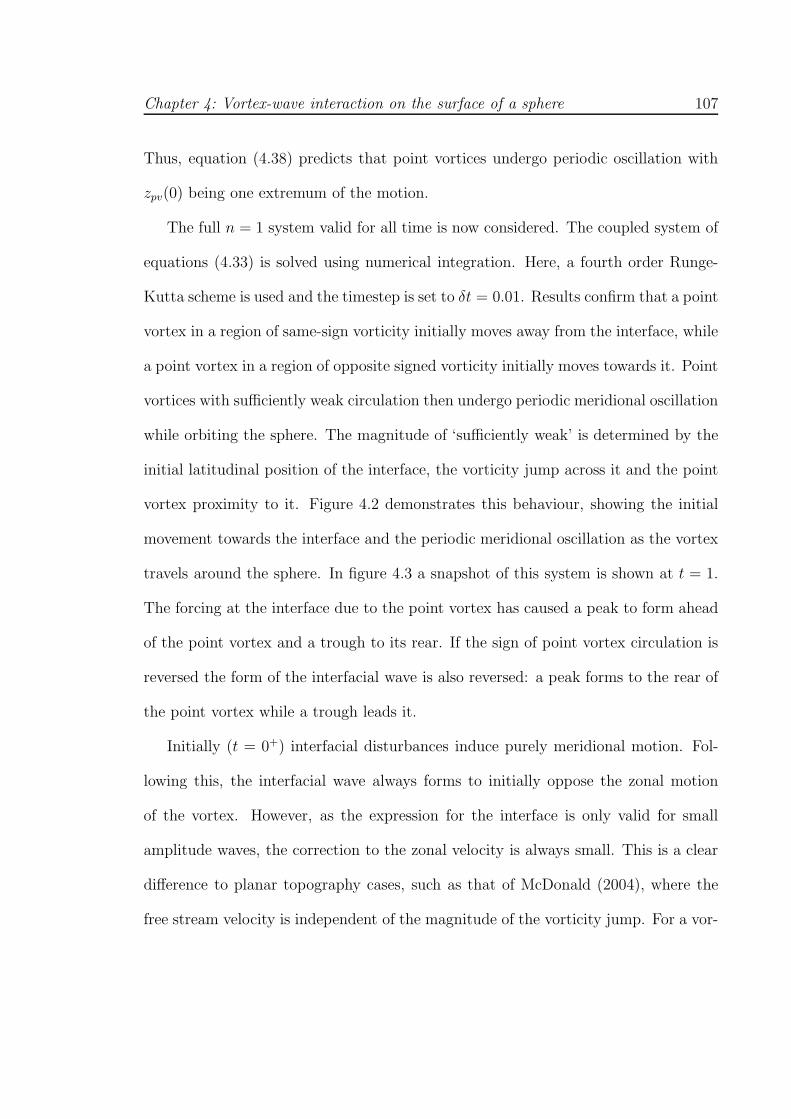
Chapter 4: Vortex-wave interaction on the surface of a sphere 107
Thus, equation (4.38) predicts that point vortices undergo periodic oscillation with
zpv(0) being one extremum of the motion.
The full n = 1 system valid for all time is now considered. The coupled system of
equations (4.33) is solved using numerical integration. Here, a fourth order Runge-
Kutta scheme is used and the timestep is set to δt = 0.01. Results confirm that a point
vortex in a region of same-sign vorticity initially moves away from the interface, while
a point vortex in a region of opposite signed vorticity initially moves towards it. Point
vortices with sufficiently weak circulation then undergo periodic meridional oscillation
while orbiting the sphere. The magnitude of ‘sufficiently weak’ is determined by the
initial latitudinal position of the interface, the vorticity jump across it and the point
vortex proximity to it. Figure 4.2 demonstrates this behaviour, showing the initial
movement towards the interface and the periodic meridional oscillation as the vortex
travels around the sphere. In figure 4.3 a snapshot of this system is shown at t = 1.
The forcing at the interface due to the point vortex has caused a peak to form ahead
of the point vortex and a trough to its rear. If the sign of point vortex circulation is
reversed the form of the interfacial wave is also reversed: a peak forms to the rear of
the point vortex while a trough leads it.
Initially (t = 0+) interfacial disturbances induce purely meridional motion. Fol-
lowing this, the interfacial wave always forms to initially oppose the zonal motion
of the vortex. However, as the expression for the interface is only valid for small
amplitude waves, the correction to the zonal velocity is always small. This is a clear
difference to planar topography cases, such as that of McDonald (2004), where the
free stream velocity is independent of the magnitude of the vorticity jump. For a vor-
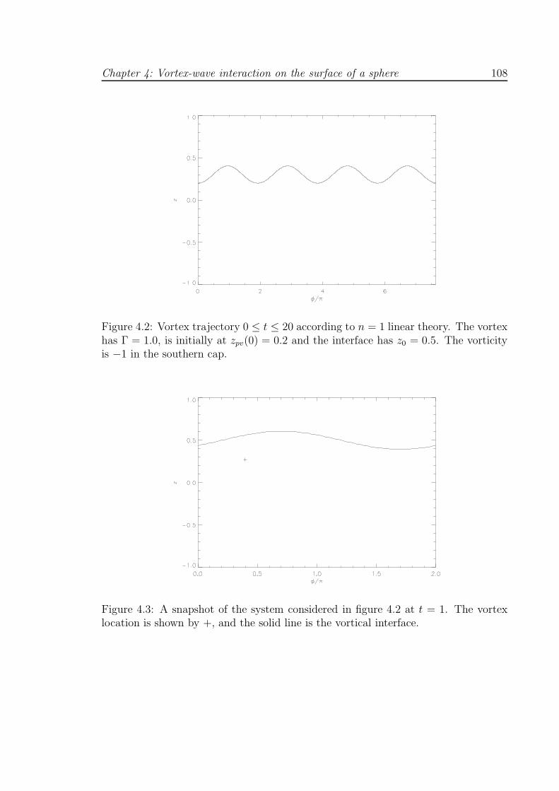
Chapter 4: Vortex-wave interaction on the surface of a sphere 108
Figure 4.2: Vortex trajectory 0 ≤ t ≤ 20 according to n = 1 linear theory. The vortexhas Γ = 1.0, is initially at zpv(0) = 0.2 and the interface has z0 = 0.5. The vorticityis −1 in the southern cap.
Figure 4.3: A snapshot of the system considered in figure 4.2 at t = 1. The vortexlocation is shown by +, and the solid line is the vortical interface.
Chapter 4: Vortex-wave interaction on the surface of a sphere 109
tical interface on the sphere, the unperturbed angular velocity, Ω0, and that due to
interfacial perturbations are proportional to the vorticity jump ω across the interface.
This means that a low Ω0 can only result in a weak correction to the zonal flow.
The long time behaviour of the system shown in figure 4.2 was examined up to
times of t ≈ 1000. The motion seen in figure 4.2 persists for these very large times
demonstrating the stability of the system. This is a characteristic of all systems
within this regime i.e. if a configuration is such that the vortex undergoes meridional
oscillation, this oscillation will persist for long periods of time.
When a strong point vortex is in a region of the same signed vorticity, the vortex
will rapidly move away from the interface towards the pole. It is simple to show from
(4.17) that these polar locations are equilibria e.g. if zpv < z0 then when zpv = −1
(the South Pole) a1 = b1 = zpv = 0 and when zpv > z0 then zpv = 1 (the North
Pole) again gives a1 = b1 = zpv = 0. Further, (4.38) indicates that a point vortex
located at a pole in a region of same sign vorticity will be a stable equilibrium. Slight
meridional perturbations to the vortex will result in a velocity at the vortex pushing
it back towards the pole. On the other hand, polar vortices in regions of opposite
signed vorticity are unstable equilibria, since perturbations away from the pole will
induce a meridional velocity pulling the vortex away from the pole.
Linear theory also predicts that if a point vortex in a region of same signed vorticity
is sufficiently strong, it will always reach the pole regardless of its initial proximity
to the vorticity interface. Clearly, for a strong vortex within close proximity to the
interface, large amplitude waves will quickly develop on the interface invalidating
linear theory. This result is therefore not expected to hold true in fully non-linear
Chapter 4: Vortex-wave interaction on the surface of a sphere 110
computations. Figure 4.4 shows the trajectory of a point vortex in this regime and
figure 4.5 the corresponding contour at t = 1. In the linear n = 1 calculation, the
vortex passes below z = −1 and then proceeds to oscillate, never returning above
z = −1. Clearly the trajectory is non-physical once the vortex has passed below
z = −1. Nevertheless, the result still gives insight into the stability of vortices in
polar regions and the initial movements of strong point vortices in these regions.
The interface of figure 4.5 is ‘opposite’ in shape to that of 4.3 owing to the different
sign circulation of the vortex i.e. a trough now precedes the vortex. Also, owing
to the large circulation of the vortex, large amplitude waves have developed upon
the interface. For strong point vortices in regions of opposite signed vorticity, linear
theory breaks down as the point vortex rapidly approaches the interface exciting large
amplitude disturbances, and then ‘crossing’ the interface.
4.3 Truncating at n > 1
In this section, the effect of truncating (4.16), (4.17), (4.29) and (4.32) at n > 1
on the resulting dynamics is examined. As in section 4.2, the system of 2N + 2
ODEs resulting from truncating at n = N is solved numerically using a fourth order
Runge-Kutta scheme with timestep δt = 0.01.
Truncating at n > 1 alters the dynamics to varying degrees according to the
vortex strength, vorticity jump across the interface and the vortices proximity to
the interface. Figure 4.6 compares vortex trajectories for solutions truncated at n =
1, n = 3 and n = 50 for a weak vortex initially at a reasonable distance from the
interface. This is a highly linear case and, as expected, the three trajectories are very
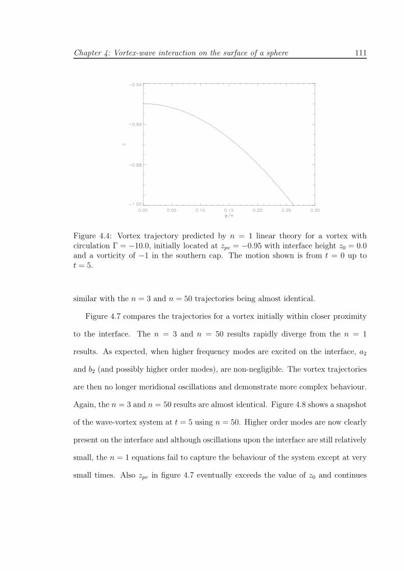
Chapter 4: Vortex-wave interaction on the surface of a sphere 111
Figure 4.4: Vortex trajectory predicted by n = 1 linear theory for a vortex withcirculation Γ = −10.0, initially located at zpv = −0.95 with interface height z0 = 0.0and a vorticity of −1 in the southern cap. The motion shown is from t = 0 up tot = 5.
similar with the n = 3 and n = 50 trajectories being almost identical.
Figure 4.7 compares the trajectories for a vortex initially within closer proximity
to the interface. The n = 3 and n = 50 results rapidly diverge from the n = 1
results. As expected, when higher frequency modes are excited on the interface, a2
and b2 (and possibly higher order modes), are non-negligible. The vortex trajectories
are then no longer meridional oscillations and demonstrate more complex behaviour.
Again, the n = 3 and n = 50 results are almost identical. Figure 4.8 shows a snapshot
of the wave-vortex system at t = 5 using n = 50. Higher order modes are now clearly
present on the interface and although oscillations upon the interface are still relatively
small, the n = 1 equations fail to capture the behaviour of the system except at very
small times. Also zpv in figure 4.7 eventually exceeds the value of z0 and continues
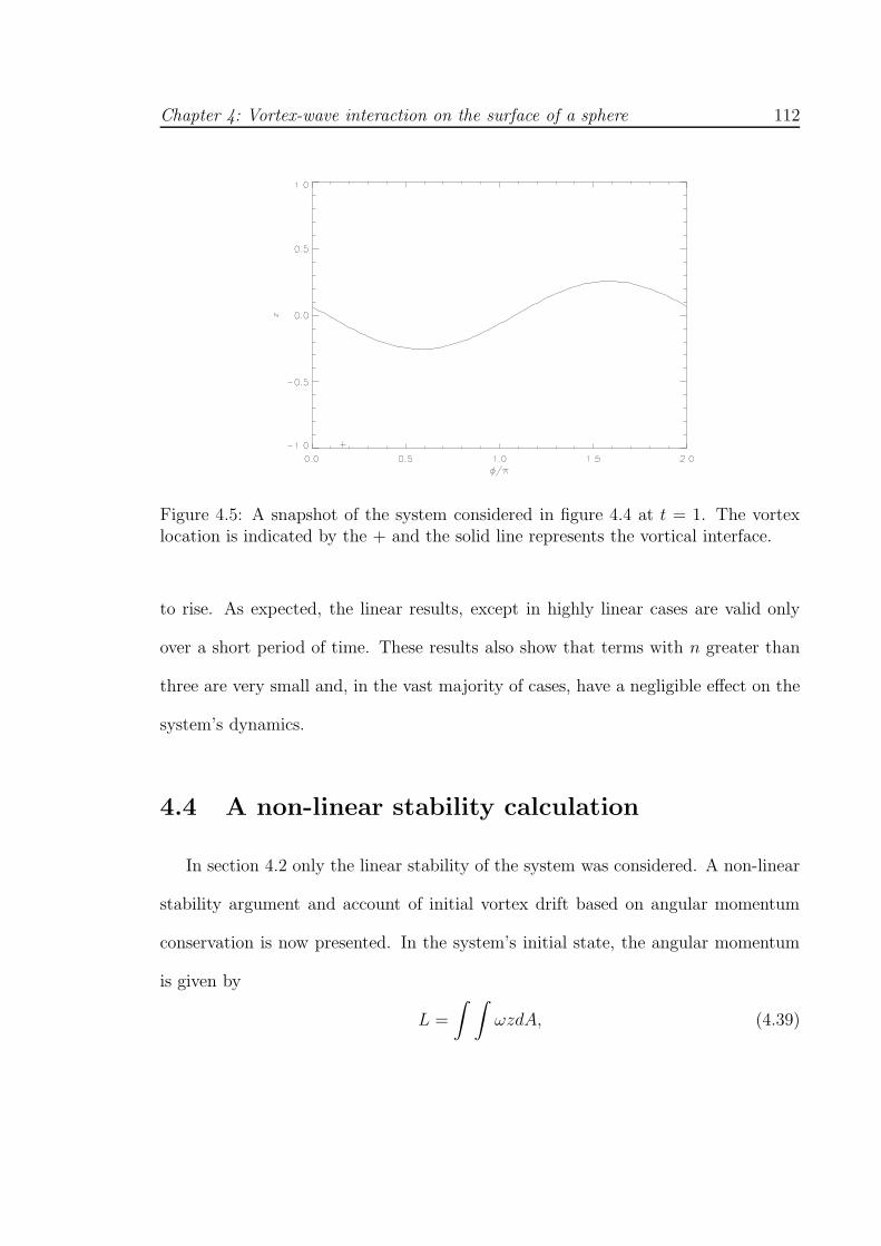
Chapter 4: Vortex-wave interaction on the surface of a sphere 112
Figure 4.5: A snapshot of the system considered in figure 4.4 at t = 1. The vortexlocation is indicated by the + and the solid line represents the vortical interface.
to rise. As expected, the linear results, except in highly linear cases are valid only
over a short period of time. These results also show that terms with n greater than
three are very small and, in the vast majority of cases, have a negligible effect on the
system’s dynamics.
4.4 A non-linear stability calculation
In section 4.2 only the linear stability of the system was considered. A non-linear
stability argument and account of initial vortex drift based on angular momentum
conservation is now presented. In the system’s initial state, the angular momentum
is given by
L =
∫ ∫
ωzdA, (4.39)
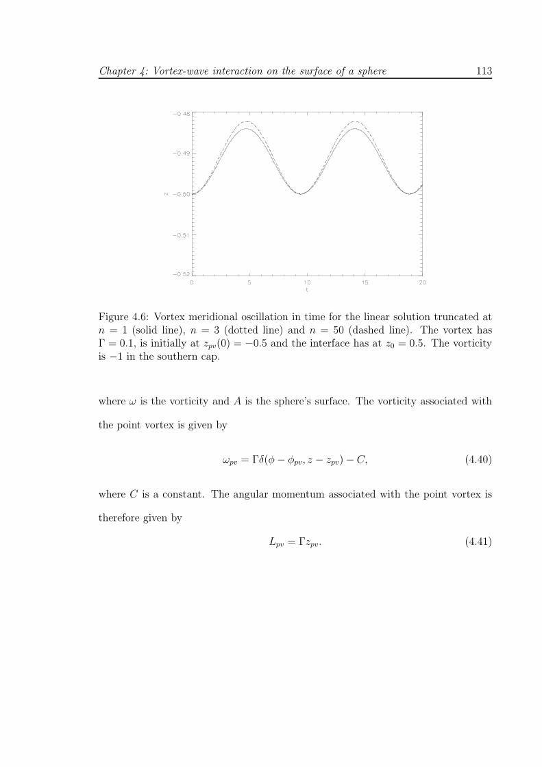
Chapter 4: Vortex-wave interaction on the surface of a sphere 113
Figure 4.6: Vortex meridional oscillation in time for the linear solution truncated atn = 1 (solid line), n = 3 (dotted line) and n = 50 (dashed line). The vortex hasΓ = 0.1, is initially at zpv(0) = −0.5 and the interface has at z0 = 0.5. The vorticityis −1 in the southern cap.
where ω is the vorticity and A is the sphere’s surface. The vorticity associated with
the point vortex is given by
ωpv = Γδ(φ− φpv, z − zpv) − C, (4.40)
where C is a constant. The angular momentum associated with the point vortex is
therefore given by
Lpv = Γzpv. (4.41)
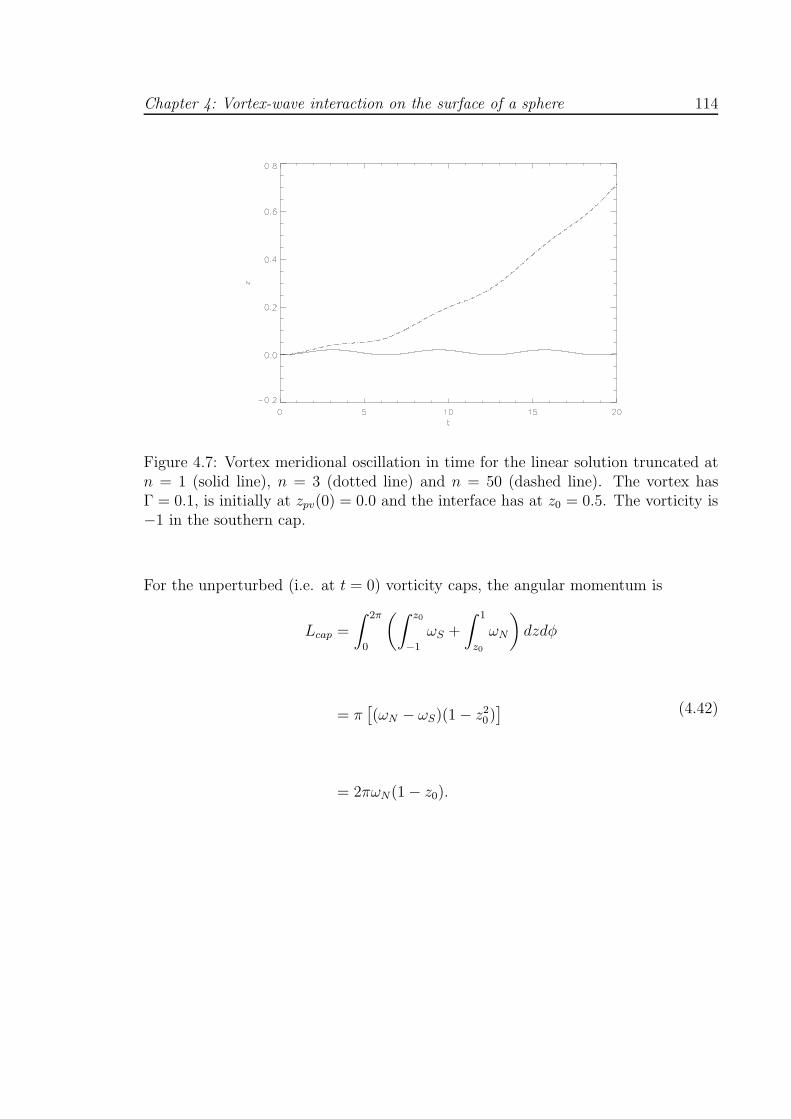
Chapter 4: Vortex-wave interaction on the surface of a sphere 114
Figure 4.7: Vortex meridional oscillation in time for the linear solution truncated atn = 1 (solid line), n = 3 (dotted line) and n = 50 (dashed line). The vortex hasΓ = 0.1, is initially at zpv(0) = 0.0 and the interface has at z0 = 0.5. The vorticity is−1 in the southern cap.
For the unperturbed (i.e. at t = 0) vorticity caps, the angular momentum is
Lcap =
∫ 2π
0
(∫ z0
−1
ωS +
∫ 1
z0
ωN
)
dzdφ
= π[
(ωN − ωS)(1 − z20)]
= 2πωN(1 − z0).
(4.42)
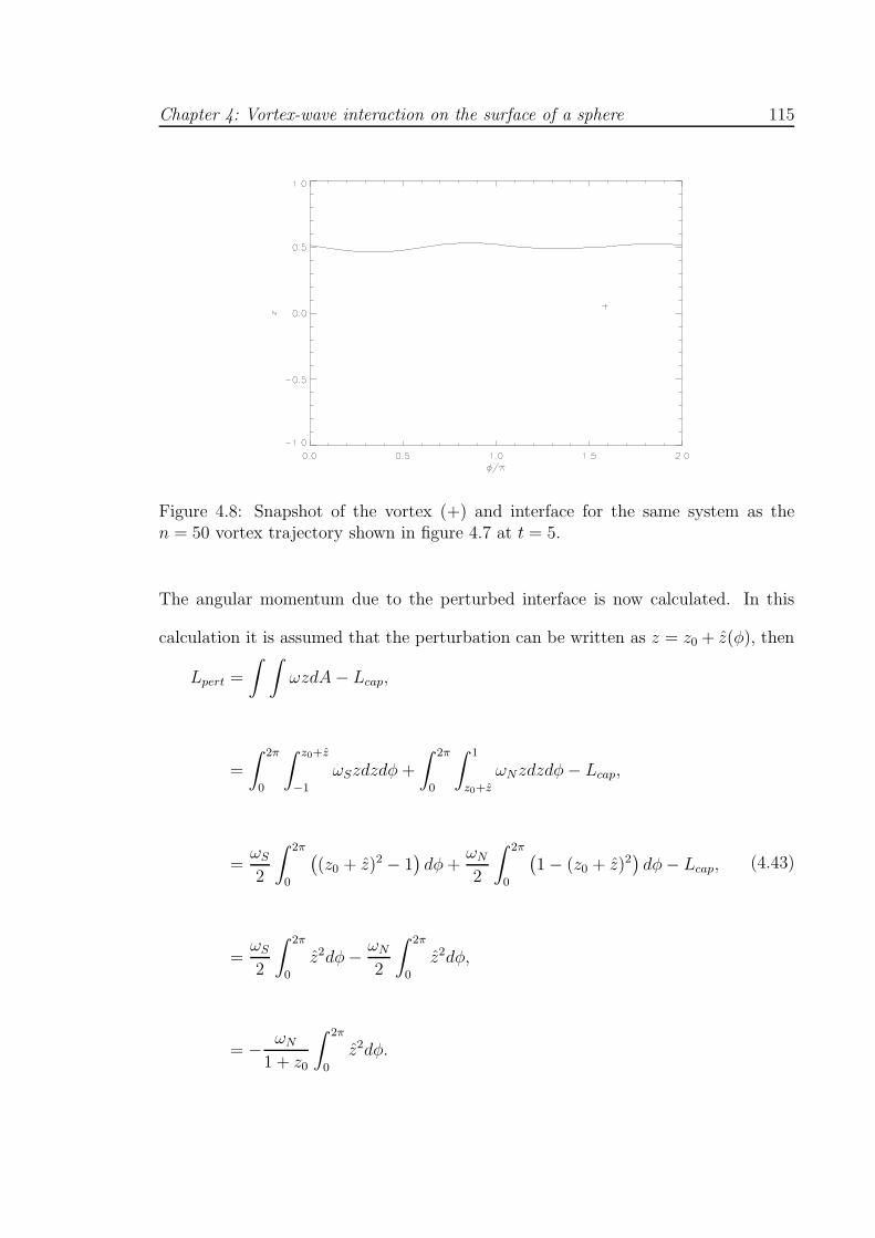
Chapter 4: Vortex-wave interaction on the surface of a sphere 115
Figure 4.8: Snapshot of the vortex (+) and interface for the same system as then = 50 vortex trajectory shown in figure 4.7 at t = 5.
The angular momentum due to the perturbed interface is now calculated. In this
calculation it is assumed that the perturbation can be written as z = z0 + z(φ), then
Lpert =
∫ ∫
ωzdA− Lcap,
=
∫ 2π
0
∫ z0+z
−1
ωSzdzdφ +
∫ 2π
0
∫ 1
z0+z
ωNzdzdφ− Lcap,
=ωS
2
∫ 2π
0
(
(z0 + z)2 − 1)
dφ+ωN
2
∫ 2π
0
(
1 − (z0 + z)2)
dφ− Lcap,
=ωS
2
∫ 2π
0
z2dφ− ωN
2
∫ 2π
0
z2dφ,
= − ωN
1 + z0
∫ 2π
0
z2dφ.
(4.43)
Chapter 4: Vortex-wave interaction on the surface of a sphere 116
In order to examine the stability of the system it is first shown that L is constant.
From (4.39)
L =
∫ 2π
0
∫ π2
−π2
ω cos θ sin θdθdφ
=
∫ 2π
0
∫ π2
−π2
(
sin θ∂
∂θ
(
cos θ∂ψ
∂θ
)
+ tan θ∂2ψ
∂φ2
)
dθdφ
= −∫ 2π
0
∫ π2
−π2
cos2 θ∂ψ
∂θdθdφ,
(4.44)
from the periodicity in the system. But u = −∂ψ/∂θ and thus
L =
∫ 2π
0
∫ π2
−π2
u cos2 θdθdφ
=
∫ ∫
u cos θdA ≡ Ltotal,
(4.45)
where Ltotal is the total angular momentum which is a conserved quantity in the
system. Ltotal=Lpv + Lcap + Lpert (where Lcap = constant) and thus from equations
(4.42) and (4.43) there are two cases to consider: (i) Γ > 0, ωN > 0 and (ii) Γ < 0,
ωN > 0. For (i), if the disturbance amplitude at the interface increases then according
to (4.43) Lpert decreases and thus Lpv must increase, meaning zpv increases. Therefore
a positive vortex at the North Pole is stable and a positive vortex at the South
Pole unstable. For case (ii), again, if the amplitude of the interface increases, Lpert
will decrease and thus Lpv must again increase meaning zpv must decrease. There
is therefore stability for a negative vortex at the South Pole and instability for a
negative vortex at the North Pole.
Chapter 4: Vortex-wave interaction on the surface of a sphere 117
These calculations reinforce the results obtained from linear theory and demon-
strate that even in non-linear regimes, provided the interface can be written as
z = z0 + z(φ) (i.e. the interface does not become a multi-valued function of φ),
the poles are stable equilibrium locations for vortices in regions of the same sign
vorticity and unstable for vortices in regions of opposite sign vorticity.
In the following section the results of linear theory are used to verify time-
dependent non-linear contour dynamics results. Vortex trajectories obtained from
contour dynamics will be tested against those predicted by linear theory. Following
this, more ‘exotic’ non-linear behaviour will be considered.
4.5 Non-linear computations
The results of the linear theory presented in sections 4.2 and 4.3 are now used to
validate computations using the contour dynamics algorithm (Dritschel 1988). The
algorithm is described in appendix A. In the following computations, the resolution
parameter between nodes was set to 0.01 and time integration is carried out using a
fourth-order Runge-Kutta scheme with timestep δt = 0.01. Following each timestep,
the interfacial nodes are redistributed according to the local curvature meaning that,
even for highly non-linear cases, accurate vortex trajectories and interface shapes can
be computed.
Figure 4.9 displays the vortex trajectories computed using contour dynamics and
those given by n = 100 linear theory for the highly linear case previously considered
in section 4.6, that is, Γ = 0.1, zpv(0) = −0.5, z0 = 0.5 and ωS = −1 for time up
to t ≈ 20. There is excellent agreement between linear theory and contour dynamics
Chapter 4: Vortex-wave interaction on the surface of a sphere 118
in this case. When a large number of terms are included in the linear analysis, the
trajectories are almost identical over long time scales. Figure 4.10 then shows a
comparison of the vortex trajectories given by n = 100 linear theory and contour
dynamics for a more non-linear system: the system considered in figure 4.7 with
Γ = 0.1, zpv(0) = 0.0, z0 = 0.5 and ωS = −1. Linear theory and contour dynamics
are in very good agreement up to t ≈ 5. However, for time greater than t = 5 the
trajectories begin to diverge. From t ≈ 11 onwards the trajectories diverge rapidly
and linear theory completely fails to capture the non-linear motion. Linear theory
predicts that the vortex continues to rise towards the interface, whereas contour
dynamics predicts that after the initial movement of the vortex towards the interface,
it then begins to move away from it.
For systems with moderate strength point vortices, where the waves on the inter-
face can no longer be considered linear, but remain single-valued with respect to the
azimuthal coordinate φ, a point vortex in a region of same/opposite sign vorticity will
undergo periodic oscillation with a mean drift away/towards the contour depending
on the sign of their vorticity relative to the surrounding fluid (see for example the
vortex trajectory in figure 4.11 for a case when the drift is away from the interface).
Vortices in regions of opposite sign vorticity that drift towards the contour eventually
come within close proximity of the contour and induce highly nonlinear wrapping of
the contour. Vortices in regions of same signed vorticity drift away from the contour
and towards the pole with the rate of drift decreasing as the vortex moves further
away from the contour. The system, in effect, becomes more linear as relative dis-
tance between vortex and contour increases. In moderate strength vortex systems,
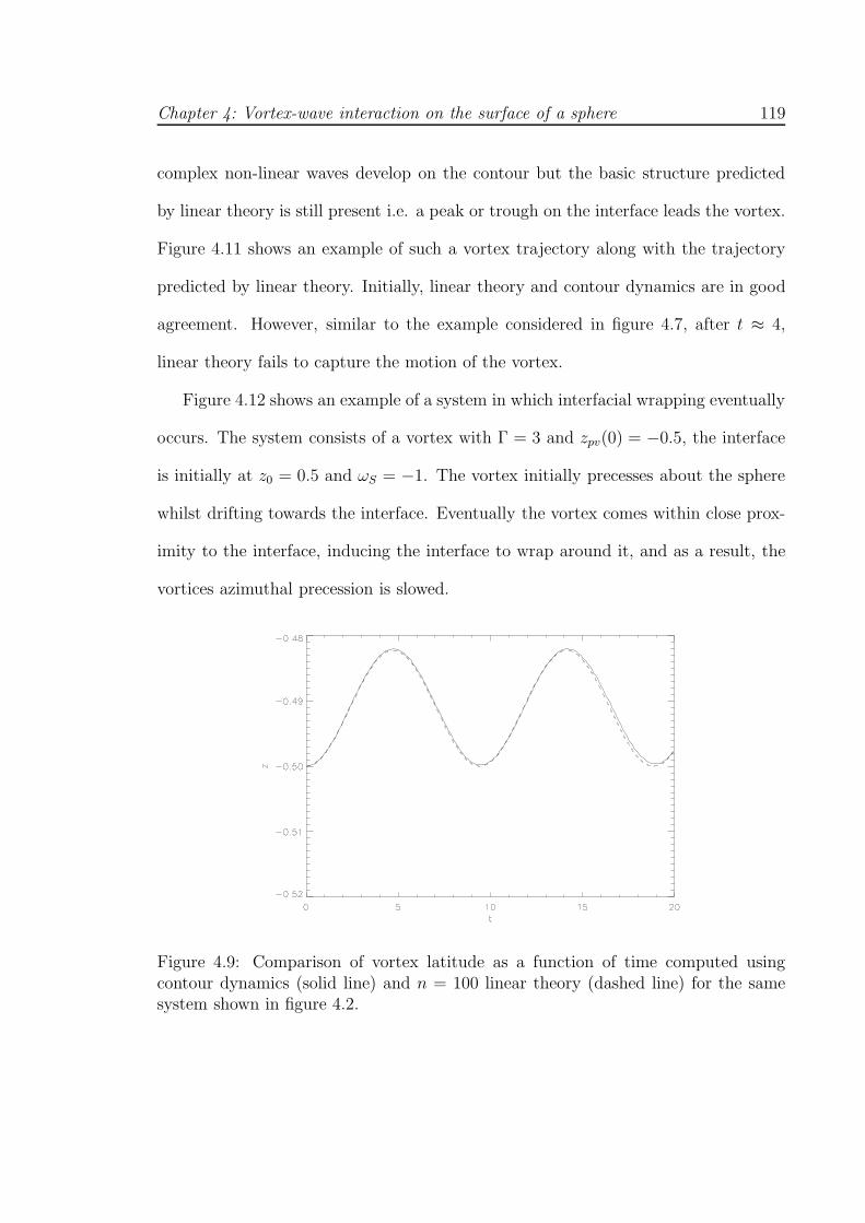
Chapter 4: Vortex-wave interaction on the surface of a sphere 119
complex non-linear waves develop on the contour but the basic structure predicted
by linear theory is still present i.e. a peak or trough on the interface leads the vortex.
Figure 4.11 shows an example of such a vortex trajectory along with the trajectory
predicted by linear theory. Initially, linear theory and contour dynamics are in good
agreement. However, similar to the example considered in figure 4.7, after t ≈ 4,
linear theory fails to capture the motion of the vortex.
Figure 4.12 shows an example of a system in which interfacial wrapping eventually
occurs. The system consists of a vortex with Γ = 3 and zpv(0) = −0.5, the interface
is initially at z0 = 0.5 and ωS = −1. The vortex initially precesses about the sphere
whilst drifting towards the interface. Eventually the vortex comes within close prox-
imity to the interface, inducing the interface to wrap around it, and as a result, the
vortices azimuthal precession is slowed.
Figure 4.9: Comparison of vortex latitude as a function of time computed usingcontour dynamics (solid line) and n = 100 linear theory (dashed line) for the samesystem shown in figure 4.2.
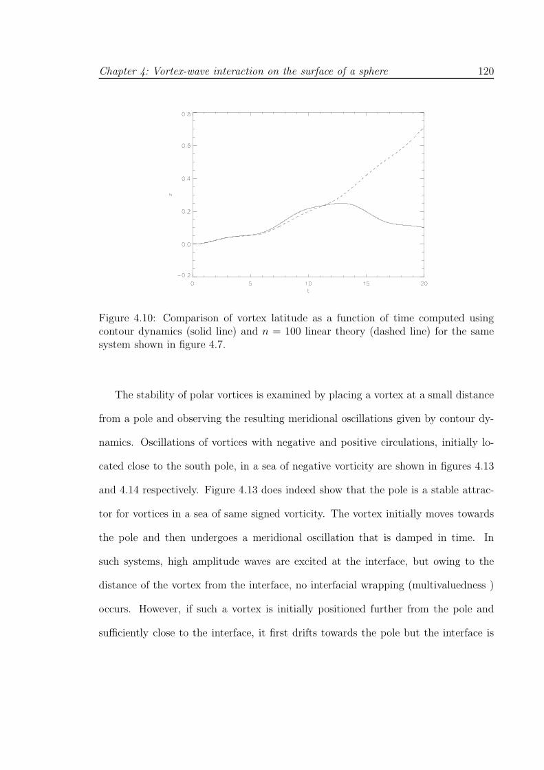
Chapter 4: Vortex-wave interaction on the surface of a sphere 120
Figure 4.10: Comparison of vortex latitude as a function of time computed usingcontour dynamics (solid line) and n = 100 linear theory (dashed line) for the samesystem shown in figure 4.7.
The stability of polar vortices is examined by placing a vortex at a small distance
from a pole and observing the resulting meridional oscillations given by contour dy-
namics. Oscillations of vortices with negative and positive circulations, initially lo-
cated close to the south pole, in a sea of negative vorticity are shown in figures 4.13
and 4.14 respectively. Figure 4.13 does indeed show that the pole is a stable attrac-
tor for vortices in a sea of same signed vorticity. The vortex initially moves towards
the pole and then undergoes a meridional oscillation that is damped in time. In
such systems, high amplitude waves are excited at the interface, but owing to the
distance of the vortex from the interface, no interfacial wrapping (multivaluedness )
occurs. However, if such a vortex is initially positioned further from the pole and
sufficiently close to the interface, it first drifts towards the pole but the interface is
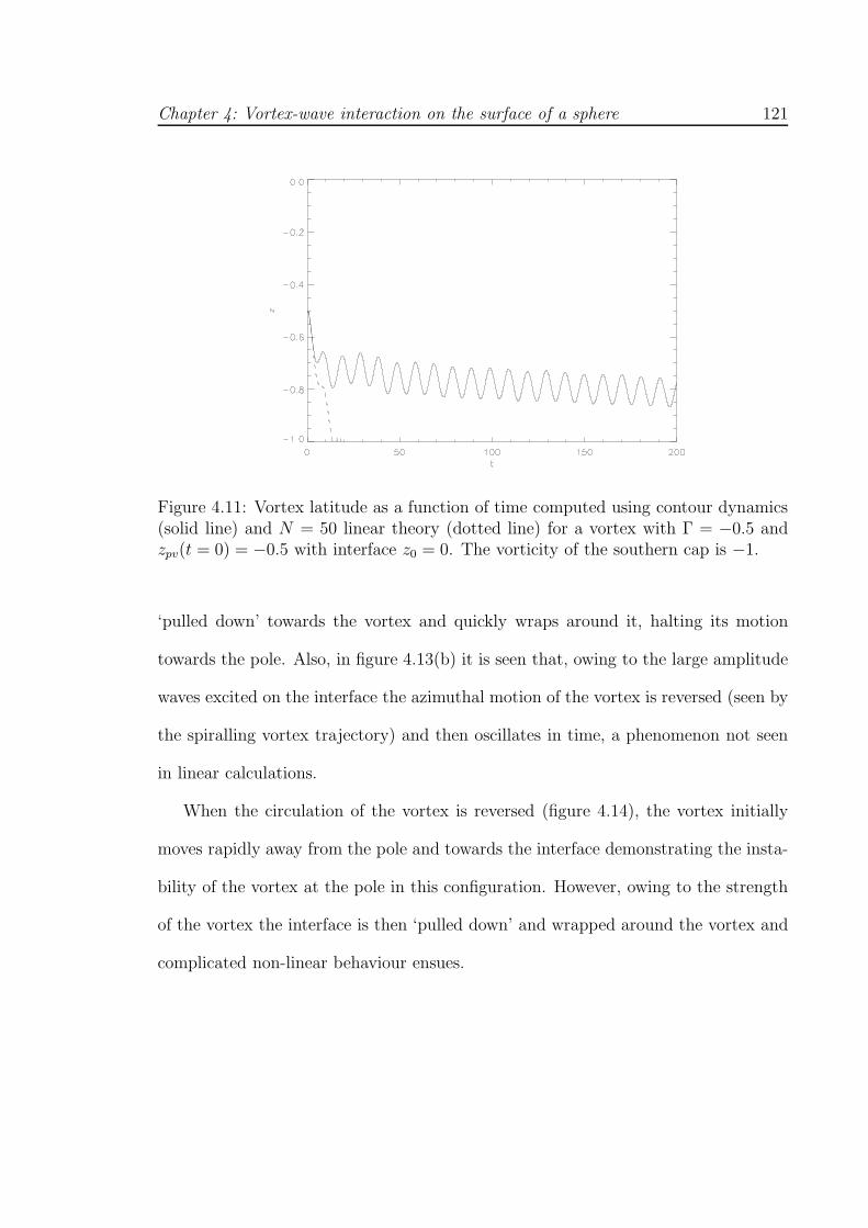
Chapter 4: Vortex-wave interaction on the surface of a sphere 121
Figure 4.11: Vortex latitude as a function of time computed using contour dynamics(solid line) and N = 50 linear theory (dotted line) for a vortex with Γ = −0.5 andzpv(t = 0) = −0.5 with interface z0 = 0. The vorticity of the southern cap is −1.
‘pulled down’ towards the vortex and quickly wraps around it, halting its motion
towards the pole. Also, in figure 4.13(b) it is seen that, owing to the large amplitude
waves excited on the interface the azimuthal motion of the vortex is reversed (seen by
the spiralling vortex trajectory) and then oscillates in time, a phenomenon not seen
in linear calculations.
When the circulation of the vortex is reversed (figure 4.14), the vortex initially
moves rapidly away from the pole and towards the interface demonstrating the insta-
bility of the vortex at the pole in this configuration. However, owing to the strength
of the vortex the interface is then ‘pulled down’ and wrapped around the vortex and
complicated non-linear behaviour ensues.
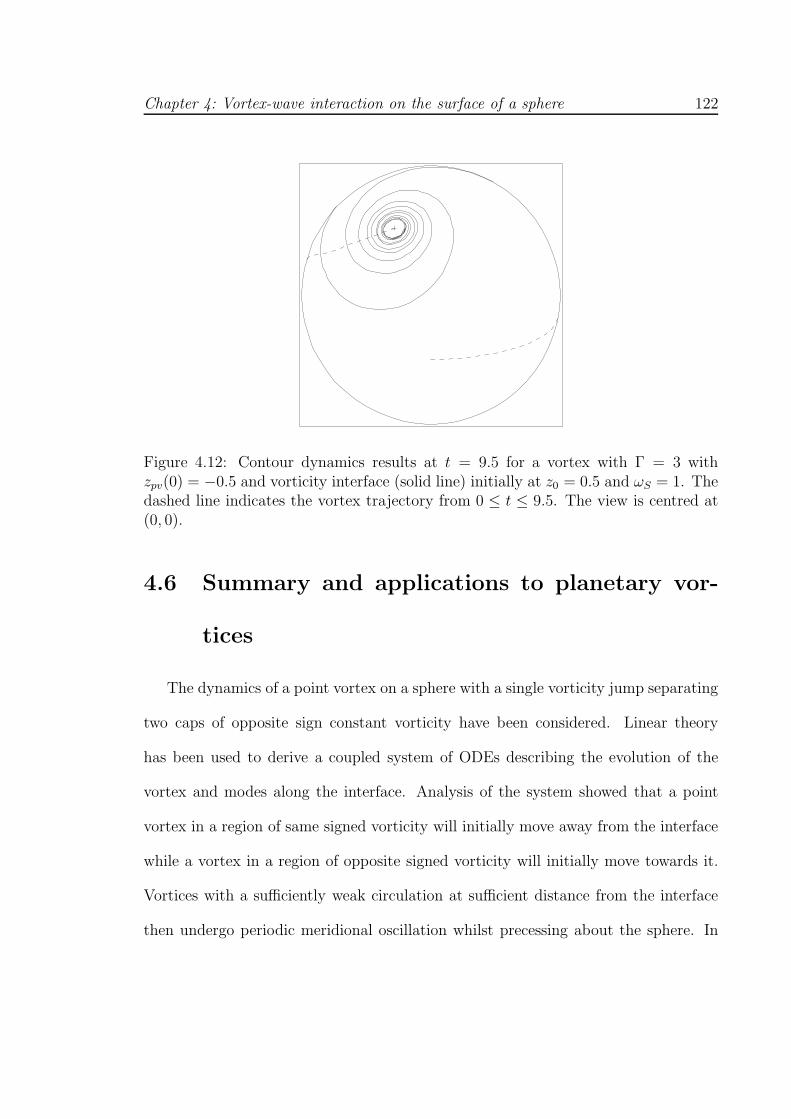
Chapter 4: Vortex-wave interaction on the surface of a sphere 122
Figure 4.12: Contour dynamics results at t = 9.5 for a vortex with Γ = 3 withzpv(0) = −0.5 and vorticity interface (solid line) initially at z0 = 0.5 and ωS = 1. Thedashed line indicates the vortex trajectory from 0 ≤ t ≤ 9.5. The view is centred at(0, 0).
4.6 Summary and applications to planetary vor-
tices
The dynamics of a point vortex on a sphere with a single vorticity jump separating
two caps of opposite sign constant vorticity have been considered. Linear theory
has been used to derive a coupled system of ODEs describing the evolution of the
vortex and modes along the interface. Analysis of the system showed that a point
vortex in a region of same signed vorticity will initially move away from the interface
while a vortex in a region of opposite signed vorticity will initially move towards it.
Vortices with a sufficiently weak circulation at sufficient distance from the interface
then undergo periodic meridional oscillation whilst precessing about the sphere. In
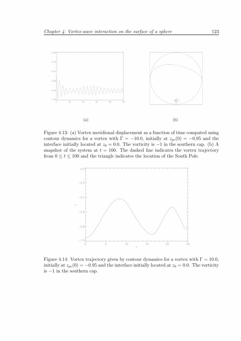
Chapter 4: Vortex-wave interaction on the surface of a sphere 123
(a) (b)
Figure 4.13: (a) Vortex meridional displacement as a function of time computed usingcontour dynamics for a vortex with Γ = −10.0, initially at zpv(0) = −0.95 and theinterface initially located at z0 = 0.0. The vorticity is −1 in the southern cap. (b) Asnapshot of the system at t = 100. The dashed line indicates the vortex trajectoryfrom 0 ≤ t ≤ 100 and the triangle indicates the location of the South Pole.
Figure 4.14: Vortex trajectory given by contour dynamics for a vortex with Γ = 10.0,initially at zpv(0) = −0.95 and the interface initially located at z0 = 0.0. The vorticityis −1 in the southern cap.
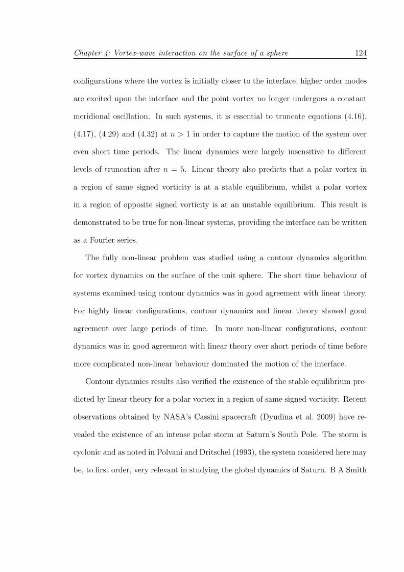
Chapter 4: Vortex-wave interaction on the surface of a sphere 124
configurations where the vortex is initially closer to the interface, higher order modes
are excited upon the interface and the point vortex no longer undergoes a constant
meridional oscillation. In such systems, it is essential to truncate equations (4.16),
(4.17), (4.29) and (4.32) at n > 1 in order to capture the motion of the system over
even short time periods. The linear dynamics were largely insensitive to different
levels of truncation after n = 5. Linear theory also predicts that a polar vortex in
a region of same signed vorticity is at a stable equilibrium, whilst a polar vortex
in a region of opposite signed vorticity is at an unstable equilibrium. This result is
demonstrated to be true for non-linear systems, providing the interface can be written
as a Fourier series.
The fully non-linear problem was studied using a contour dynamics algorithm
for vortex dynamics on the surface of the unit sphere. The short time behaviour of
systems examined using contour dynamics was in good agreement with linear theory.
For highly linear configurations, contour dynamics and linear theory showed good
agreement over large periods of time. In more non-linear configurations, contour
dynamics was in good agreement with linear theory over short periods of time before
more complicated non-linear behaviour dominated the motion of the interface.
Contour dynamics results also verified the existence of the stable equilibrium pre-
dicted by linear theory for a polar vortex in a region of same signed vorticity. Recent
observations obtained by NASA’s Cassini spacecraft (Dyudina et al. 2009) have re-
vealed the existence of an intense polar storm at Saturn’s South Pole. The storm is
cyclonic and as noted in Polvani and Dritschel (1993), the system considered here may
be, to first order, very relevant in studying the global dynamics of Saturn. B A Smith

Chapter 4: Vortex-wave interaction on the surface of a sphere 125
(1982) points to evidence suggesting that on Saturn there exists a so called zonal
‘ribbon’ with a strong vorticity gradient near the equator. The global circulation is
anticyclonic to the north of the ribbon and cyclonic to its south resulting in the mean
winds at the equator being generally to the east. There is therefore the possibility
that there exists a strong cyclonic storm surrounded by a cyclonic sea i.e. the polar
storm has the same signed vorticity as its surrounding fluid. As discussed previously
in this chapter, for a cyclonic southern cap, the South Pole would be a stable equilib-
rium for a cyclonic storm such as the one observed at Saturn’s South Pole. This result
therefore offers a possible dynamic explanation explaining the presence and stability
of Saturn’s polar storm.
Systems with moderate strength vortices displayed a variety of possible behaviour.
One characteristic of such systems was that the vortex would generally drift away
from the interface if surrounded by a sea of same signed vorticity and towards it if
surrounded by a sea of opposite signed vorticity. For vortices surrounded by seas of
same signed vorticity, the rate of drift away from the interface would decrease with
distance from the interface and the vortex trajectory would slowly settle down into
a meridional oscillation while precessing around the sphere. As mentioned above,
vortices in seas of opposite signed vorticity drift towards the interface resulting in
the amplitude of disturbances at the interface growing as the vortex gets closer.
Generally, the vortex would get within close enough proximity of the interface to
eventually induce wrapping, thus halting the meridional drift of the vortex.
Chapter 5
Finite area vortex motion on a
sphere with impenetrable
boundaries
Vortex motion in the presence of impenetrable boundaries is an important problem
in vortex dynamics due to its relevance in modeling geophysical flows, especially
oceanographic flows. Oceanic eddies frequently interact with topography such as
ridges and coastlines, the resulting interactions can play an important role in ocean
circulation and various other ocean processes. For example, With such motivation in
mind, Pedlosky (1994) models the flow of the stratified abyssal ocean in the presence
of a partial meridional (north-south) barrier, Sheremet (2001) the passage of a western
boundary current across a gap and Nof (1995) the rotating exchange flow through a
narrow gap between large-scale ocean basins. Since deep ocean vortices, observed to
exist at depths up to 4km (McWilliams 1985), can propagate large distances they will
126
Chapter 5: Finite area vortex motion on a sphere with impenetrable boundaries 127
frequently encounter mid-ocean ridges occurring at similar depths (e.g. the Walvis
Ridge in the South Atlantic). Due to their role in ocean circulation and the transport
of tracers, understanding the circumstances in which they are able to penetrate gaps
in ridges is important. In addition to deep ocean vortex-topography interactions,
surface trapped vortex structures also frequently interact with complex topography.
One such example is the collision of North Brazil Current Rings with the Lesser
Antilles (Fratantoni et al. 1995). For large-scale vortex structures, the curvature
of the Earth can play a significant role in the evolution of the system. Hence it is
desirable to develop methods that accurately compute vortex behaviour on the surface
of a sphere.
For problems involving vortex motion in planar bounded domains governed by the
two-dimensional Euler equations with the vorticity distribution chosen such that it is
a singular point in the domain (a point vortex), progress can be made using conformal
mapping techniques. Provided a conformal mapping exists between the domain and
a relatively simpler domain in which a vortex Hamiltonian (Kirchhoff-Routh path
function) (Saffman 1992) can be constructed, this Hamiltonian along with information
from the mapping gives the Hamiltonian in the original domain from which the vortex
trajectory can be deduced. Such point vortex systems can give a good indication of
the dynamics of a vortex patch with constant vorticity, especially when the boundary
of a vortex remains close to circular since the velocity field exterior to a circular
vortex patch is identical to that of a point vortex with the same circulation. However,
in many geophysical systems it is of interest to consider cases in which the vorticity
distribution is not singular but a finite region of vorticity which is able to deform, and
Chapter 5: Finite area vortex motion on a sphere with impenetrable boundaries 128
when in close proximity to solid objects or other regions of vorticity can filament or
even split. The conformal mapping method is not directly applicable to such cases as a
finite area vortex patch is governed by Poisson’s equation which is not invariant under
conformal mapping. The dynamics exterior to the vortex are, however, governed by
Laplace’s equation and are hence invariant under conformal mapping. Thus, provided
the vorticity distributions being considered are piece-wise constant, contour dynamics
(Dritschel 1989) along with the invariance of the irrotational exterior flow under
conformal mapping can be utilized to examine such systems. Johnson and McDonald
(2004a) consider the planar problem of a point vortex near a gap in a plate with
and without ambient flows for which exact solutions of point vortex trajectories are
obtained through deriving the appropriate vortex Hamiltonian. In the absence of
ambient flows a vortex travelling towards the gap will pass through the gap and
travel back along the other side of the plate if its far-field distance from the plate is
less than half the gap width. Otherwise the vortex will leap across the gap. A method
for computing the motion of finite area patches of constant vorticity near such a gap
for which the invariance of the irrotational exterior flow under conformal mapping
and the numerical method of contour dynamics are utilized are then presented. When
the vortex boundary remains close to circular the centroid of the patch follows that
of the point vortex trajectory very closely. Cases in which the vortex is ‘pinched’
against the gap edge can lead to filamentation and even vortex splitting can occur.
This method is extended to study the motion of point vortices and vortex patches
near two circular cylinders of arbitrary radii (Johnson and McDonald 2004b) and near
a barrier with two collinear gaps (Johnson and McDonald 2005). For point vortices,
Chapter 5: Finite area vortex motion on a sphere with impenetrable boundaries 129
Crowdy and Marshall (2005) generalized the study of Johnson and McDonald (2004b)
to domains of arbitrary connectivity, presenting a method for constructing a vortex
Hamiltonian in a bounded or unbounded domain containing an arbitrary number of
cylinders of arbitrary radii. The method of Crowdy and Marshall (2005) is used to
study the motion of a point vortex through gaps in walls in Crowdy and Marshall
(2006). Trajectories about gaps in a wall off a coastline and in an unbounded ocean
are considered. Some results from Johnson and McDonald (2005) are reproduced and
extended to domains of higher connectivity. In a recent study, Crowdy and Surana
(2008) present a method for implementing contour dynamics in planar domains of
arbitrary connectivity based on constructing the Green’s function in a pre-image
circular domain. Various examples are presented including the motion of a patch
near an infinite wall, a gap in a wall and in a circular basin with multiple circular
islands.
For planetary scale geophysical flows, it is clearly of interest to consider such
problems on the surface of a sphere. As mentioned in chapter 4, moving from the plane
to the sphere introduces new effects into the problem. The periodicity of the sphere
introduces a ‘feed back’ effect and the curvature of the sphere can introduce ‘shielding’
effects. In the absence of topography on the sphere it is required that the total
vorticity on the surface of the sphere is equal to zero: the Gauss integral constraint.
Point vortex motion on the surface of the sphere in the presence of impenetrable
boundaries is considered in the studies of Kidambi and Newton (2000) and Crowdy
(2006). Kidambi and Newton (2000) use the method of images to derive exact point
vortex trajectories for a spherical cap, longitudinal wedge, half-longitudinal wedge,
Chapter 5: Finite area vortex motion on a sphere with impenetrable boundaries 130
channel and rectangle. Due to limitations of the method of images, solutions for the
wedge, half-wedge and rectangle are restricted to bounded geometries between the
azimuthal angles of φ = 0 and φ = π/m where m is a positive integer. Crowdy (2006)
presents a formulation based on a generalization of the Kirchhoff-Routh path function
to the surface of a sphere, abandoning the need for special symmetries demanded by
the method of images. The analog of the ‘gap in a wall’ problem of Johnson and
McDonald (2004a) on the surface of a sphere is also considered. The impenetrable
barrier considered lies along a great circle with longitude (or azimuthal angle) φ =
0, π except for a single, symmetrical gap centred about the south pole for θ ≥ θ0
where 0 ≤ θ ≤ π is the co-latitude. For θ0 less than 0.6082π the south pole is an
elliptic stationary point of the Hamiltonian in contrast to the planar case in which the
centre of the gap is always a hyperbolic stationary point of the Hamiltonian (Johnson
and McDonald 2004a). When θ0 exceeds this value a quantitative change in vortex
behavior occurs and the Hamiltonian has a hyperbolic stationary point at the south
pole and two symmetrical elliptic stationary points emerge at right angles to the
plate. As θ0 is increased further the curvature of the spherical surface plays a lesser
role in the dynamics in the vicinity of the gap and trajectories resemble those of the
planar case close to the gap (Johnson and McDonald 2004a).
In the absence of impenetrable boundaries Dritschel (1988) extends the method of
contour dynamics to the surface of a sphere. This method is has been used to model
waves and vortices on a sphere (in the absence of boundaries) and compute steadily
rotating vortex structures (Dritschel and Polvani 1992; Polvani and Dritschel 1993).
This chapter considers the motion of finite area patches of constant vorticity on
Chapter 5: Finite area vortex motion on a sphere with impenetrable boundaries 131
the non-rotating unit sphere with impenetrable boundaries. Techniques described
in Johnson and McDonald (2004a) and Johnson and McDonald (2005) are extended
to the surface of the sphere and used to examine vortex patch motion in bounded
domains which is then compared to the exact point vortex trajectories (Crowdy 2006).
The domains considered include the exterior to an ellipse of semimajor axis a and
semiminor axis b in the stereographic plane, a longitudinal wedge and half-longitudinal
wedge bounded between zero and an angle φ (where 0 < φ < 2π) and a thin barrier
with two gaps. For the case when the semiminor axis of the ellipse is equal to zero (i.e.
a gap in a plate, Crowdy 2006) the motion of the patch with compatible background
flows is also considered.
As discussed above, Crowdy (2006) shows when the boundary is a gap in a plate,
the point vortex Hamiltonian has an elliptic stationary point located symmetrically
between the two plate edges (provided θ0 < 0.6082π). Thus, the possibility of stable
steady vortices (V-states) located between the gap arises. Families of vortex equilibria
for different gap widths are computed using a numerical method based on that of
Pierrehumbert (1980) and their stability investigated.
Surana and Crowdy (2008) have also considered the motion of vortex patches on
a sphere in the presence of boundaries using a modification of the method of Crowdy
and Surana (2008). Their method also uses stereographic projection of the physical
region of interest and also the patch itself (unlike in this work). They then conformally
map to a canonical circular domain and use the results of Crowdy and Surana (2008)
to show that a contour dynamics formulation exists.
The approach of presented in this chapter is complementary to that of Surana and
Chapter 5: Finite area vortex motion on a sphere with impenetrable boundaries 132
Crowdy (2008). It has the advantage of being straightforward to implement using a
‘standard’ contour dynamics routine on a sphere although here it is restricted (unlike
Surana and Crowdy 2008) to singly and doubly connected domains. However, the
method can, in principle, be used to tackle domains of any connectivity provided the
region of interest can be mapped to a circular domain consisting of the unit disk with
smaller circular disks excised in which the corresponding boundary value problem
can be solved to obtain the appropriate irrotational flow field. The range of examples
considered here complement those of Surana and Crowdy (2008). Additionally in
this chapter background flows are considered, point vortex and patch trajectories are
compared and a family of vortex equilibria residing in a gap are computed.
5.1 Contour dynamics in singly connected domains
on a sphere
The system consists of a shallow layer of constant depth, incompressible and
inviscid fluid in a simply connected bounded domain D on the surface of the unit
sphere. Let Ψ denote the total streamfunction due to a finite number of vortices
(with piecewise constant vorticity) in the domain D such that the no-normal flow
boundary condition
Ψ = 0 on ∂D, (5.1)
is satisfied. Further, let ψ1 be the streamfunction owing to the vortices in the absence
of boundaries ∂D, which gives
uθ = − 1
sin θ
∂ψ1
∂φ, uφ =
∂ψ1
∂θ, (5.2)
Chapter 5: Finite area vortex motion on a sphere with impenetrable boundaries 133
where φ ∈ [0, 2π) is the azimuthal angle and θ ∈ [0, π] is the latitudinal angle and uφ
and uθ are the zonal and latitudinal velocities respectively. Velocities on ∂D owing
to ψ1 are computed using the method of contour dynamics (Dritschel 1988, 1989).
Introduce an irrotational flow, with streamfunction ψ0, defined throughout D such
that
Ψ = ψ1 + ψ0. (5.3)
The no-normal-flow condition on the boundary ∂D requires that
d(ψ1 + ψ0) = 0, (5.4)
and hence from (5.2) the relationship between the irrotational flow field and that
induced by the vortices in D on ∂D is given by
∂ψ0
∂θdθ +
∂ψ0
∂θdφ = −
(
∂ψ1
∂θdθ +
∂ψ1
∂θdφ
)
= −uφdθ + uθ sin θdφ. (5.5)
Introduce the stereographic projection into the complex z-plane such that
z = cot
(
θ
2
)
eiφ, (5.6)
which conformally maps ∂D to ∂Dz with the north pole being mapped to ∞ and the
south pole to the origin of the z-plane. Velocities in the projected z-plane related to
those on the sphere can be obtained by direct differentiation of (5.6) giving
u(z) − iv(z) = −ir(1 + r2)
2z(uφ − uθ), (5.7)
where r = |z|. The following two results for a point vortex in the stereographic plane
with zero net circulation are useful (Kidambi and Newton 2000)
Chapter 5: Finite area vortex motion on a sphere with impenetrable boundaries 134
1. The velocity field induced by a point vortex of strength Γ in the stereographic
plane is
u(z) − iv(z) =(1 + r2)2
4
[
− i
2π
Γ
z − zα
]
, (5.8)
where r = |z| and zα is the position of the point vortex in the stereographic
plane.
2. The velocity field felt by the vortex in the stereographic plane is
u(z)α − iv(z)
α = − iΓ
8π(1 + r2
α)zα. (5.9)
Importantly, note that in (5.8), only the term in the square brackets is confor-
mally invariant.
The first step in incorporating boundaries in the contour dynamics algorithm is to
compute the velocities uφ and uθ on the boundary ∂D using a standard contour
dynamics algorithm for a sphere (i.e. as if boundaries were not present). A contour
dynamics algorithm formulated on the surface of the sphere (appendix A.1) is used to
find the equivalent velocities on ∂Dz , u(z) − iu(z). Note that stereographic projection
is conformal and so preserves the angle between the velocity vector and the tangent
to the boundary: this property being important when constructing an irrotational
flow field that when added to u(z) − iv(z) gives zero normal flow on the boundary.
Next, a velocity field u(z) − iv(z) is to be found, such that when added to u(z) −
iv(z) the normal component of the resulting velocity field vanishes on ∂Dz and, by
conformality of the stereographic projection, on ∂D. It is required that u(z) − iv(z) is
irrotational on the sphere so no extra vorticity is being added to the dynamics.
Chapter 5: Finite area vortex motion on a sphere with impenetrable boundaries 135
To determine u(z) − iv(z), Dz is mapped to the exterior unit circle Dζ in the ζ-
plane using the map ζ = F (z). Importantly, the velocity data u(z) − iv(z) on ∂Dz is
divided by the factor (1 + r2)/4 (see (5.8)) since it is required that the velocity field
be conformally invariant under this map. Let the velocity field on ∂Dz be u(z)c − iv
(z)c
after dividing by this factor. Requiring that the total component of u(z)c − iv
(z)c and
u(z)c − iv
(z)c normal to ∂Dz vanishes gives
ℑ[(u(z)c − iv(z)
c )dz]∂Dz= −ℑ[(u(z)
c − iv(z)c )dz]∂Dz
. (5.10)
On ∂Dζ , ζ = eiσ (0 ≤ σ < 2π) and noting dw = (u(z)c − iv
(z)c )dz, (5.10) can be written
as
ℑ[
dw
dσ
]
∂Dζ
= −ℑ[
iζ
F ′(z)(u(z)
c − iv(z)c )
]
∂Dζ
= g(σ), (5.11)
where g(σ) is a known function on ∂Dζ and w is the complex potential of the velocity
field sought.
Let
w = iC log ζ +
∞∑
k=1
akζ−k (5.12)
where C ∈ R and ak are complex constants. The constant C determines the circula-
tion around the obstacle and is arbitrary. Expressing g(σ) as a Fourier series, ak can
be determined efficiently by Fast Fourier Transforms. Thus (5.12) gives
u(z) − iv(z) =(1 + r2)2
4
dw
dζ
dζ
dz=
(1 + r2)2
4
[
iC
ζ+
∞∑
k=1
−kakζ−k−1
]
F ′(z). (5.13)
The velocity correction on the sphere is, using (5.7),
uφ − iuθ =2iz
r(1 + r2)(u(z) − iv(z)). (5.14)
Chapter 5: Finite area vortex motion on a sphere with impenetrable boundaries 136
Since u(z)−iv(z) is irrotational in the z-plane it is possible to show by direct calculation
that uφ − iuθ given by (5.14) is indeed irrotational on the sphere.
Finally, to advect points on the contour the following three velocity fields are
required:
(i) the self-induced velocity owing to the vorticity of the patch (or patches) itself.
(ii) the velocity correction uφ − iuθ given by (5.14).
(iii) the velocity given by (5.9), where zα is now zi, the ith node of the patch bound-
ary.
To compute (iii) it is necessary to compute Γ = ωA where A is the patch area. This
can be done efficiently using boundary data using the boundary integral expression
A =
∮
∂B
(1 − z)dφ, (5.15)
where z = r cos θ and ∂B is the patch boundary. Additionally, the patch centroid
position given by
X =T
|T| , (5.16)
where T =∮
∂Bx × dx, is calculated for later use in comparison of patch trajectories
with those of point vortices.
In practice the sum in (5.13) is truncated at some valueN . Vortex patches in D are
then advected using a fourth order Runge-Kutta method. The procedure presented
in this section is then repeated at the beginning of each time step.
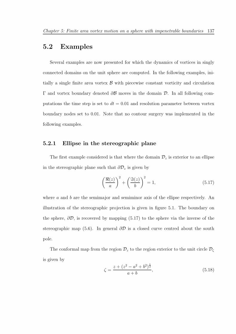
Chapter 5: Finite area vortex motion on a sphere with impenetrable boundaries 137
5.2 Examples
Several examples are now presented for which the dynamics of vortices in singly
connected domains on the unit sphere are computed. In the following examples, ini-
tially a single finite area vortex B with piecewise constant vorticity and circulation
Γ and vortex boundary denoted ∂B moves in the domain D. In all following com-
putations the time step is set to dt = 0.01 and resolution parameter between vortex
boundary nodes set to 0.01. Note that no contour surgery was implemented in the
following examples.
5.2.1 Ellipse in the stereographic plane
The first example considered is that where the domain Dz is exterior to an ellipse
in the stereographic plane such that ∂Dz is given by
(ℜ(z)
a
)2
+
(ℑ(z)
b
)2
= 1, (5.17)
where a and b are the semimajor and semiminor axis of the ellipse respectively. An
illustration of the stereographic projection is given in figure 5.1. The boundary on
the sphere, ∂D, is recovered by mapping (5.17) to the sphere via the inverse of the
stereographic map (5.6). In general ∂D is a closed curve centred about the south
pole.
The conformal map from the region Dz to the region exterior to the unit circle Dζ
is given by
ζ =z + (z2 − a2 + b2)
12
a+ b, (5.18)
Chapter 5: Finite area vortex motion on a sphere with impenetrable boundaries 138
Figure 5.1: Schematic illustraiting the stereographic projection from the sphere to anellipse in the complex z-plane.
with inverse
z =1
2
(
(a + b)ζ + (a− b)ζ−1)
. (5.19)
To ensure the vortex system on the sphere has zero net circulation the constant C is
set to be
C = − Γ
2π. (5.20)
Velocities on ∂B in D are then computed as outlined in the previous section. The
sum in equation (5.13) is truncated at N = 400.
For comparison purposes exact point vortex trajectories in the domain D in the
case where the boundary is an ellipse in the stereographic plane in the absence of a
background flow can be derived using the Kirchhoff-Routh path function for point
vortices on a sphere (Crowdy 2006) and using the maps (5.19,5.20). The point vortex
Chapter 5: Finite area vortex motion on a sphere with impenetrable boundaries 139
trajectories are given by
∣
∣
∣
∣
∣
(1 + zαzα)
(ζ(zα)ζ(zα) − 1)
2ζ(zα)2
(a− b)ζ(zα)2 − a− b
∣
∣
∣
∣
∣
= const, (5.21)
where the subscript α indicates the location of the point vortex. Figure 5.2 shows the
patch motion about an ellipse with a = 0.2 and b = 0.1 where patch is initially circular
with Γ ≈ 0.774 and vorticity ω = 10 and centroid initially located at (φco, θco) =
(0, 2/3π). In this case the motion is contained within the Southern Hemisphere. The
boundary in this case is a “short” obstacle where the north pole is an elliptic stationary
point as determined by contours of (5.21) and thus the vortex patch dynamics will
be more analogous to the motion about an isolated object in the plane and not the
“gap in a wall” problem. The patch motion remains close to circular and thus the
centroid motion of the vortex patch follows the point vortex trajectory very closely.
This orbital motion persists for long times. Figure 5.3 (with a = 4.0, b = 0.0,
Γ ≈ −3.075, ω = −10 and (φco, θco) = (0.2π, 0.25π)) shows the case for which the
ellipse is collapsed so that it is a thin barrier around a portion of a great circle. The
boundary in this case is a “long” barrier and is thus analogous to the planar problem
of the “gap in a wall” (Johnson and McDonald 2004a). In this case, as the patch
passes the edge of the barrier the patch and barrier are within closer proximity than
in the case previously considered, thus a far greater degree of distortion of the patch is
observed. Figure 5.3 shows that for this case, after the patch passes through the gap,
the distortion induced from the interaction with the barrier results in filamentation.
The vortex then proceeds in the expected way with a filament growing in time. Such
filamentation is also typical in the planar case (Johnson and McDonald 2004a).
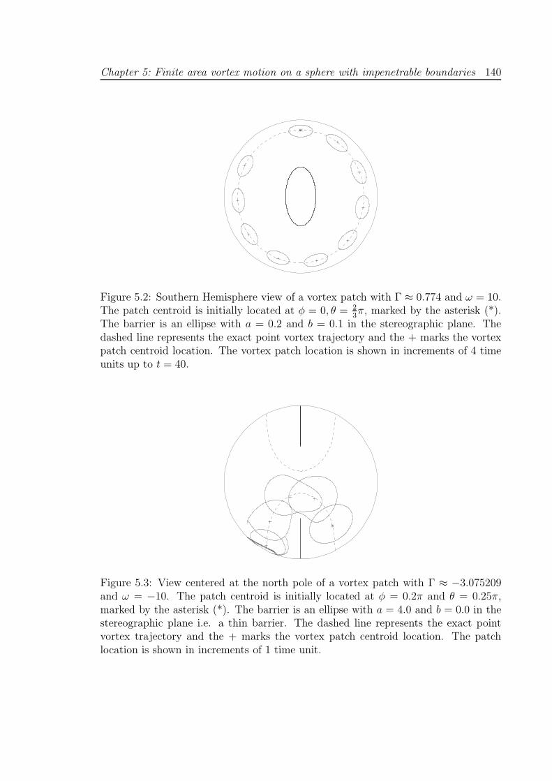
Chapter 5: Finite area vortex motion on a sphere with impenetrable boundaries 140
Figure 5.2: Southern Hemisphere view of a vortex patch with Γ ≈ 0.774 and ω = 10.The patch centroid is initially located at φ = 0, θ = 2
3π, marked by the asterisk (*).
The barrier is an ellipse with a = 0.2 and b = 0.1 in the stereographic plane. Thedashed line represents the exact point vortex trajectory and the + marks the vortexpatch centroid location. The vortex patch location is shown in increments of 4 timeunits up to t = 40.
Figure 5.3: View centered at the north pole of a vortex patch with Γ ≈ −3.075209and ω = −10. The patch centroid is initially located at φ = 0.2π and θ = 0.25π,marked by the asterisk (*). The barrier is an ellipse with a = 4.0 and b = 0.0 in thestereographic plane i.e. a thin barrier. The dashed line represents the exact pointvortex trajectory and the + marks the vortex patch centroid location. The patchlocation is shown in increments of 1 time unit.
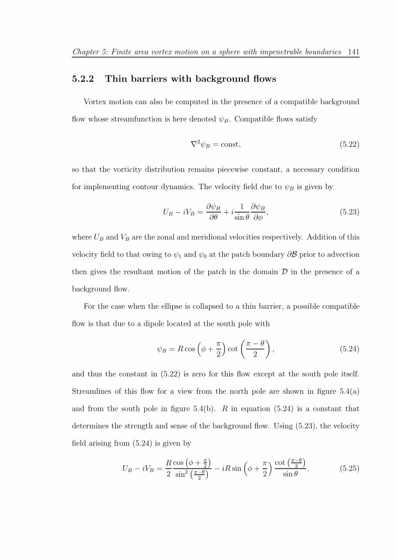
Chapter 5: Finite area vortex motion on a sphere with impenetrable boundaries 141
5.2.2 Thin barriers with background flows
Vortex motion can also be computed in the presence of a compatible background
flow whose streamfunction is here denoted ψB. Compatible flows satisfy
∇2ψB = const, (5.22)
so that the vorticity distribution remains piecewise constant, a necessary condition
for implementing contour dynamics. The velocity field due to ψB is given by
UB − iVB =∂ψB
∂θ+ i
1
sin θ
∂ψB
∂φ, (5.23)
where UB and VB are the zonal and meridional velocities respectively. Addition of this
velocity field to that owing to ψ1 and ψ0 at the patch boundary ∂B prior to advection
then gives the resultant motion of the patch in the domain D in the presence of a
background flow.
For the case when the ellipse is collapsed to a thin barrier, a possible compatible
flow is that due to a dipole located at the south pole with
ψB = R cos(
φ+π
2
)
cot
(
π − θ
2
)
, (5.24)
and thus the constant in (5.22) is zero for this flow except at the south pole itself.
Streamlines of this flow for a view from the north pole are shown in figure 5.4(a)
and from the south pole in figure 5.4(b). R in equation (5.24) is a constant that
determines the strength and sense of the background flow. Using (5.23), the velocity
field arising from (5.24) is given by
UB − iVB =R
2
cos(
φ+ π2
)
sin2(
π−θ2
) − iR sin(
φ+π
2
) cot(
π−θ2
)
sin θ. (5.25)
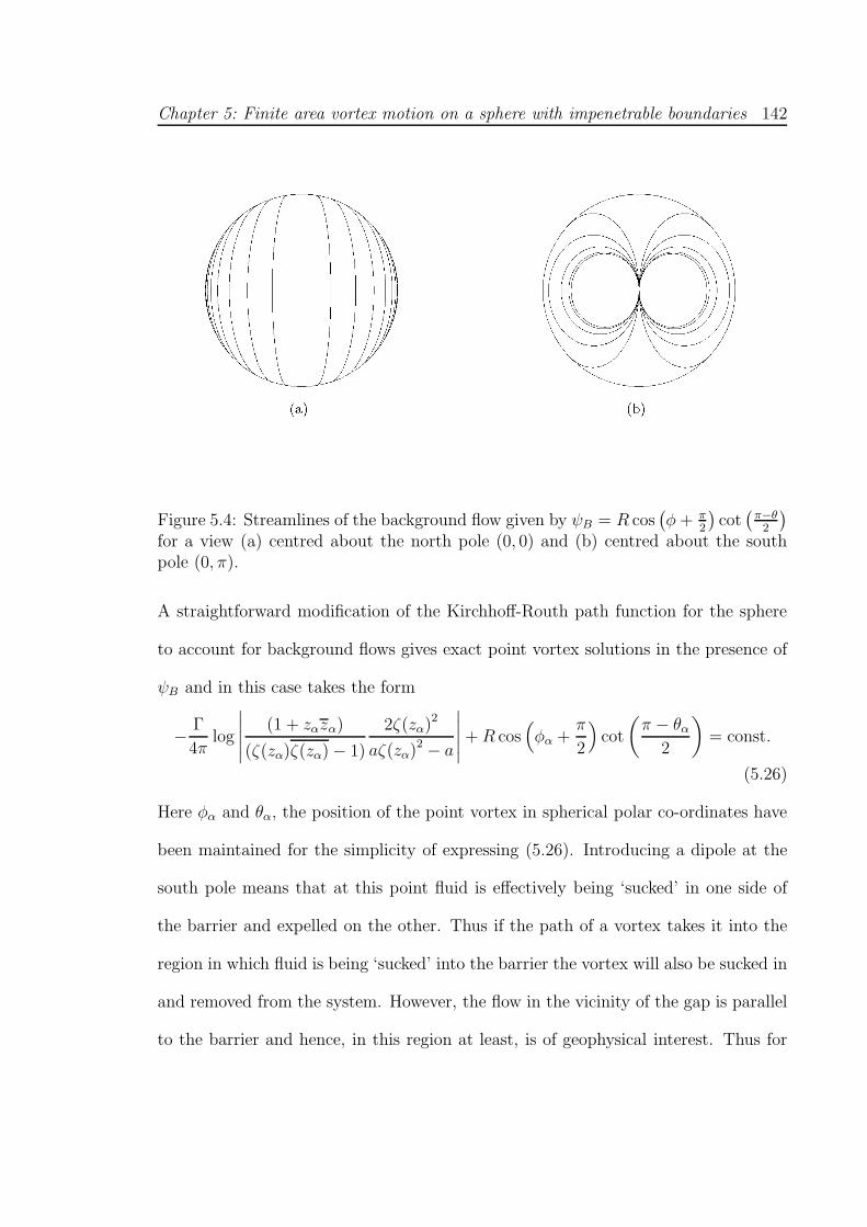
Chapter 5: Finite area vortex motion on a sphere with impenetrable boundaries 142
Figure 5.4: Streamlines of the background flow given by ψB = R cos(
φ+ π2
)
cot(
π−θ2
)
for a view (a) centred about the north pole (0, 0) and (b) centred about the southpole (0, π).
A straightforward modification of the Kirchhoff-Routh path function for the sphere
to account for background flows gives exact point vortex solutions in the presence of
ψB and in this case takes the form
− Γ
4πlog
∣
∣
∣
∣
∣
(1 + zαzα)
(ζ(zα)ζ(zα) − 1)
2ζ(zα)2
aζ(zα)2 − a
∣
∣
∣
∣
∣
+R cos(
φα +π
2
)
cot
(
π − θα
2
)
= const.
(5.26)
Here φα and θα, the position of the point vortex in spherical polar co-ordinates have
been maintained for the simplicity of expressing (5.26). Introducing a dipole at the
south pole means that at this point fluid is effectively being ‘sucked’ in one side of
the barrier and expelled on the other. Thus if the path of a vortex takes it into the
region in which fluid is being ‘sucked’ into the barrier the vortex will also be sucked in
and removed from the system. However, the flow in the vicinity of the gap is parallel
to the barrier and hence, in this region at least, is of geophysical interest. Thus for
Chapter 5: Finite area vortex motion on a sphere with impenetrable boundaries 143
this system, the period of interest is when the vortex patch interacts with the gap
and not the long term dynamics of the system. Note that in the equivalent planar
problem the dipole driving uniform flow parallel to the barrier is at infinity.
The first example considered is one in which the patch is initially located in the
gap of the barrier and to one side as shown in figure 5.5 (a = 4.0, b = 0.0, Γ ≈ −3.075,
ω = −10, (φco, θco) = (0.5π, 0.15π) and R = 5Γ/4π). The background flow is such
that it is assisting the motion of the patch towards the barrier edge. Thus as the patch
moves towards and about the plate it is ‘pinched’ against the barrier. This results in
part of the patch being pushed to the ‘left’ of the barrier and part being pushed to its
‘right’. (Where ‘left’ and ‘right’ are used in the sense of the orientation of figure 5.5.)
Following this ‘pinching’, the flow is assisting the motion of the region of the patch to
the left of the barrier and opposing the motion of the patch to its right. The patch is
thus effectively split into two separate patches whose motion becomes less coupled as
the separation between them increases. Recall that no surgery is implemented in this
algorithm and thus the ‘patches’ remain connected via a thin filament. This results
in the right hand patch having insufficient circulation to oppose the background flow
and it remains in a quasi-steady state trapped against the barrier.
Another compatible flow for the thin barrier case is that due to two fixed point vor-
tices with circulations Γa and Γb placed on the equator such that the line joining the
two point vortices is perpendicular to the barrier i.e. the vortices’ stereographically
projected fixed positions are given by za = i and zb = −i respectively. The stream-
function due to a point vortex with circulation Γ at the stereographically projected
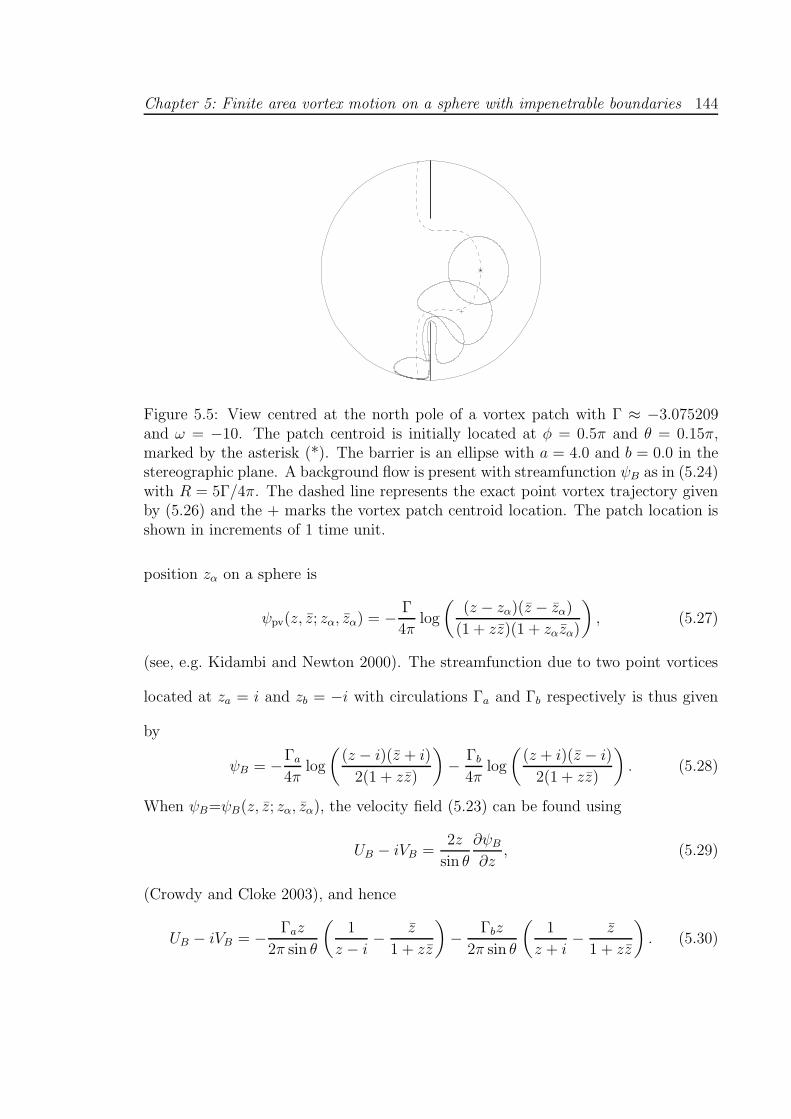
Chapter 5: Finite area vortex motion on a sphere with impenetrable boundaries 144
Figure 5.5: View centred at the north pole of a vortex patch with Γ ≈ −3.075209and ω = −10. The patch centroid is initially located at φ = 0.5π and θ = 0.15π,marked by the asterisk (*). The barrier is an ellipse with a = 4.0 and b = 0.0 in thestereographic plane. A background flow is present with streamfunction ψB as in (5.24)with R = 5Γ/4π. The dashed line represents the exact point vortex trajectory givenby (5.26) and the + marks the vortex patch centroid location. The patch location isshown in increments of 1 time unit.
position zα on a sphere is
ψpv(z, z; zα, zα) = − Γ
4πlog
(
(z − zα)(z − zα)
(1 + zz)(1 + zαzα)
)
, (5.27)
(see, e.g. Kidambi and Newton 2000). The streamfunction due to two point vortices
located at za = i and zb = −i with circulations Γa and Γb respectively is thus given
by
ψB = −Γa
4πlog
(
(z − i)(z + i)
2(1 + zz)
)
− Γb
4πlog
(
(z + i)(z − i)
2(1 + zz)
)
. (5.28)
When ψB=ψB(z, z; zα, zα), the velocity field (5.23) can be found using
UB − iVB =2z
sin θ
∂ψB
∂z, (5.29)
(Crowdy and Cloke 2003), and hence
UB − iVB = − Γaz
2π sin θ
(
1
z − i− z
1 + zz
)
− Γbz
2π sin θ
(
1
z + i− z
1 + zz
)
. (5.30)
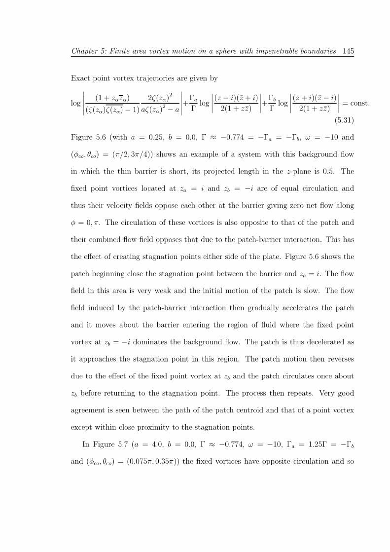
Chapter 5: Finite area vortex motion on a sphere with impenetrable boundaries 145
Exact point vortex trajectories are given by
log
∣
∣
∣
∣
∣
(1 + zαzα)
(ζ(zα)ζ(zα) − 1)
2ζ(zα)2
aζ(zα)2 − a
∣
∣
∣
∣
∣
+Γa
Γlog
∣
∣
∣
∣
(z − i)(z + i)
2(1 + zz)
∣
∣
∣
∣
+Γb
Γlog
∣
∣
∣
∣
(z + i)(z − i)
2(1 + zz)
∣
∣
∣
∣
= const.
(5.31)
Figure 5.6 (with a = 0.25, b = 0.0, Γ ≈ −0.774 = −Γa = −Γb, ω = −10 and
(φco, θco) = (π/2, 3π/4)) shows an example of a system with this background flow
in which the thin barrier is short, its projected length in the z-plane is 0.5. The
fixed point vortices located at za = i and zb = −i are of equal circulation and
thus their velocity fields oppose each other at the barrier giving zero net flow along
φ = 0, π. The circulation of these vortices is also opposite to that of the patch and
their combined flow field opposes that due to the patch-barrier interaction. This has
the effect of creating stagnation points either side of the plate. Figure 5.6 shows the
patch beginning close the stagnation point between the barrier and za = i. The flow
field in this area is very weak and the initial motion of the patch is slow. The flow
field induced by the patch-barrier interaction then gradually accelerates the patch
and it moves about the barrier entering the region of fluid where the fixed point
vortex at zb = −i dominates the background flow. The patch is thus decelerated as
it approaches the stagnation point in this region. The patch motion then reverses
due to the effect of the fixed point vortex at zb and the patch circulates once about
zb before returning to the stagnation point. The process then repeats. Very good
agreement is seen between the path of the patch centroid and that of a point vortex
except within close proximity to the stagnation points.
In Figure 5.7 (a = 4.0, b = 0.0, Γ ≈ −0.774, ω = −10, Γa = 1.25Γ = −Γb
and (φco, θco) = (0.075π, 0.35π)) the fixed vortices have opposite circulation and so
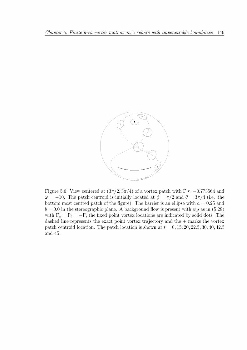
Chapter 5: Finite area vortex motion on a sphere with impenetrable boundaries 146
Figure 5.6: View centered at (3π/2, 3π/4) of a vortex patch with Γ ≈ −0.773564 andω = −10. The patch centroid is initially located at φ = π/2 and θ = 3π/4 (i.e. thebottom most centred patch of the figure). The barrier is an ellipse with a = 0.25 andb = 0.0 in the stereographic plane. A background flow is present with ψB as in (5.28)with Γa = Γb = −Γ, the fixed point vortex locations are indicated by solid dots. Thedashed line represents the exact point vortex trajectory and the + marks the vortexpatch centroid location. The patch location is shown at t = 0, 15, 20, 22.5, 30, 40, 42.5and 45.
Chapter 5: Finite area vortex motion on a sphere with impenetrable boundaries 147
reinforce each other along the barrier assisting the initial patch movement towards
the gap. The patch initially passes through the gap but the background flow field
is sufficient to overcome the patch-barrier interaction effect and advects the patch
away from the barrier. The patch then approaches the barriers opposite edge and
the resulting patch-barrier interaction results in the patch passing back through the
gap and travelling past and down the opposite edge of the barrier (on the same side
of the gap as which it begun). The patch’s interaction with the barrier results in a
deformation of the patch followed by some filamentation. Such trajectories are typical
to those seen in the planar case when a uniform background flow parallel to the barrier
is present. Johnson and McDonald (2004a) give examples in which a patch initially
passes through the gap but the background flow parallel to the barrier is sufficient to
overcome the “image” effect and results in the vortex passing back through the gap
as seen here in figure 5.7.
5.2.3 Longitudinal wedge
In Kidambi and Newton (2000) and example B of Crowdy (2006) an expression for
the trajectories of a point vortex in a longitudinal wedge bounded by the longitudes
0 and π/m for m a positive integer in Kidambi and Newton (2000) and for m a
positive real number in Crowdy (2006), were derived. Here the vortex patch motion
in such a region (with arbitrary) is computed and compared to these trajectories. As
in section 5.2.1 the region is stereographically projected into the complex plane and
then mapped to the exterior of the unit disk. Here the sum in (5.13) is truncated
to N = 800 and C is set to zero. A greater value of N is required in this (and the
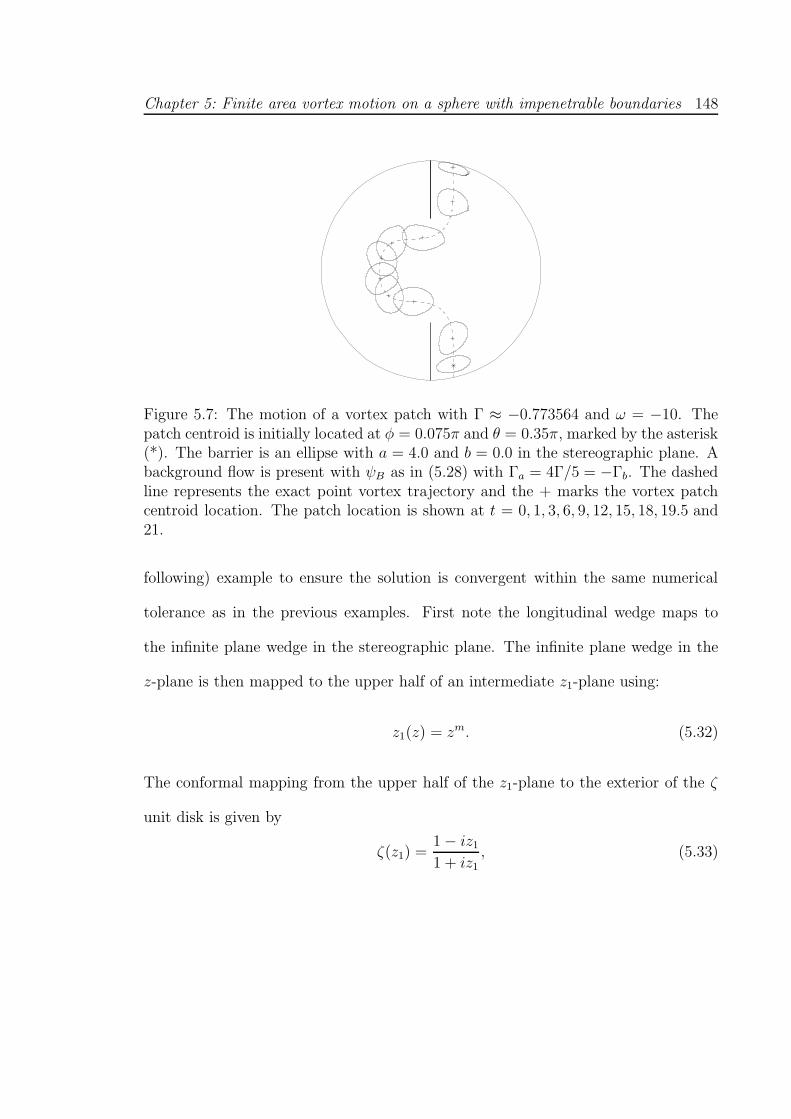
Chapter 5: Finite area vortex motion on a sphere with impenetrable boundaries 148
Figure 5.7: The motion of a vortex patch with Γ ≈ −0.773564 and ω = −10. Thepatch centroid is initially located at φ = 0.075π and θ = 0.35π, marked by the asterisk(*). The barrier is an ellipse with a = 4.0 and b = 0.0 in the stereographic plane. Abackground flow is present with ψB as in (5.28) with Γa = 4Γ/5 = −Γb. The dashedline represents the exact point vortex trajectory and the + marks the vortex patchcentroid location. The patch location is shown at t = 0, 1, 3, 6, 9, 12, 15, 18, 19.5 and21.
following) example to ensure the solution is convergent within the same numerical
tolerance as in the previous examples. First note the longitudinal wedge maps to
the infinite plane wedge in the stereographic plane. The infinite plane wedge in the
z-plane is then mapped to the upper half of an intermediate z1-plane using:
z1(z) = zm. (5.32)
The conformal mapping from the upper half of the z1-plane to the exterior of the ζ
unit disk is given by
ζ(z1) =1 − iz11 + iz1
, (5.33)
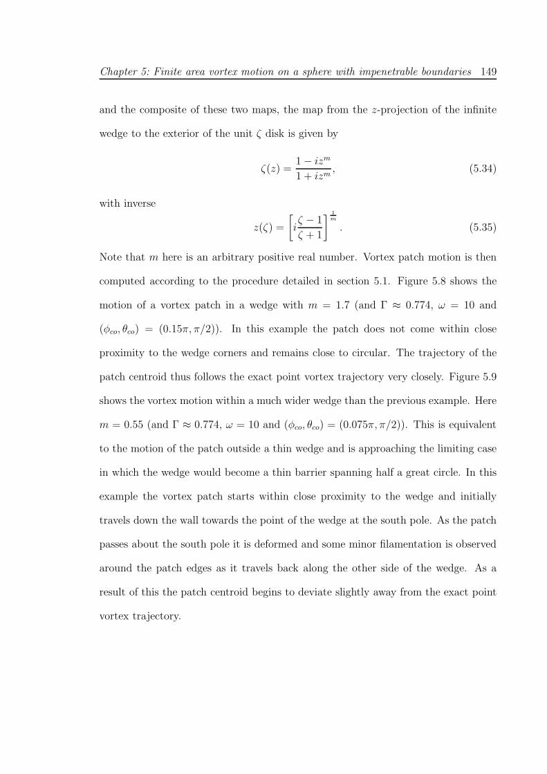
Chapter 5: Finite area vortex motion on a sphere with impenetrable boundaries 149
and the composite of these two maps, the map from the z-projection of the infinite
wedge to the exterior of the unit ζ disk is given by
ζ(z) =1 − izm
1 + izm, (5.34)
with inverse
z(ζ) =
[
iζ − 1
ζ + 1
]1m
. (5.35)
Note that m here is an arbitrary positive real number. Vortex patch motion is then
computed according to the procedure detailed in section 5.1. Figure 5.8 shows the
motion of a vortex patch in a wedge with m = 1.7 (and Γ ≈ 0.774, ω = 10 and
(φco, θco) = (0.15π, π/2)). In this example the patch does not come within close
proximity to the wedge corners and remains close to circular. The trajectory of the
patch centroid thus follows the exact point vortex trajectory very closely. Figure 5.9
shows the vortex motion within a much wider wedge than the previous example. Here
m = 0.55 (and Γ ≈ 0.774, ω = 10 and (φco, θco) = (0.075π, π/2)). This is equivalent
to the motion of the patch outside a thin wedge and is approaching the limiting case
in which the wedge would become a thin barrier spanning half a great circle. In this
example the vortex patch starts within close proximity to the wedge and initially
travels down the wall towards the point of the wedge at the south pole. As the patch
passes about the south pole it is deformed and some minor filamentation is observed
around the patch edges as it travels back along the other side of the wedge. As a
result of this the patch centroid begins to deviate slightly away from the exact point
vortex trajectory.
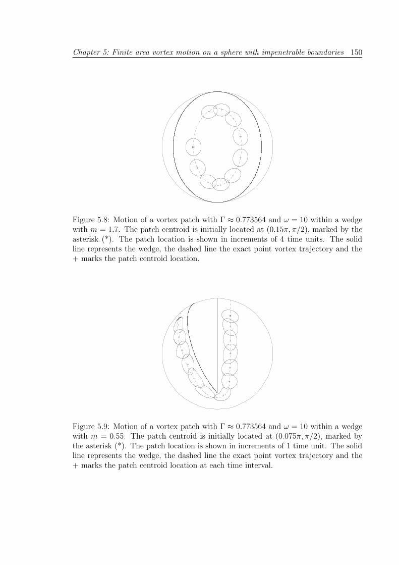
Chapter 5: Finite area vortex motion on a sphere with impenetrable boundaries 150
Figure 5.8: Motion of a vortex patch with Γ ≈ 0.773564 and ω = 10 within a wedgewith m = 1.7. The patch centroid is initially located at (0.15π, π/2), marked by theasterisk (*). The patch location is shown in increments of 4 time units. The solidline represents the wedge, the dashed line the exact point vortex trajectory and the+ marks the patch centroid location.
Figure 5.9: Motion of a vortex patch with Γ ≈ 0.773564 and ω = 10 within a wedgewith m = 0.55. The patch centroid is initially located at (0.075π, π/2), marked bythe asterisk (*). The patch location is shown in increments of 1 time unit. The solidline represents the wedge, the dashed line the exact point vortex trajectory and the+ marks the patch centroid location at each time interval.
Chapter 5: Finite area vortex motion on a sphere with impenetrable boundaries 151
5.2.4 Half-longitudinal wedge
Consider a spherical triangle domain D containing the south pole and the region
bounded by the longitudes 0 and π/m and the equator. Point vortex motion in this
geometry was also considered by Kidambi and Newton (2000) (m ∈ Z) and, more
generally, Crowdy (2006) (m ∈ R). Thus the domain Dz will be the sector of the
unit circle bounded by the lines arg(z) = 0 and arg(z) = π/m and the arc defined by
|z| = 1. C is set to zero to ensure zero circulation about the half-wedge. Next the
sector in the z-plane is mapped to the upper half of the intermediate z1-plane using
z1(z) =
(
1 + zm
1 − zm
)2
, (5.36)
followed by a map from the upper half of the z1 plane to the exterior of the unit
ζ-disk (5.33). The composite of (5.33) and (5.36) gives
ζ(z) =1 − i
(
1+zm
1−zm
)2
1 + i(
1+zm
1−zm
)2 , (5.37)
with inverse
z(ζ) =
[
i ζ−1ζ+1
]12 − 1
[
i ζ−1ζ+1
]12
+ 1
1m
. (5.38)
Figure 5.10 gives an example of the motion of a vortex patch within a half-longitudinal
wedge with m = 0.7 (and Γ ≈ 0.774, ω = 10 and (φco, θco) = (0.15π, 0.75π)) using
N = 800. The patch in this case remains close to circular and as expected the motion
of centroid matches that of a point vortex very closely.
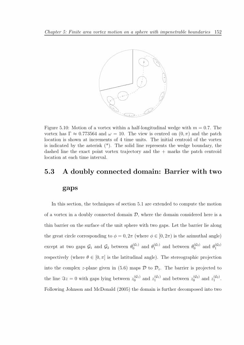
Chapter 5: Finite area vortex motion on a sphere with impenetrable boundaries 152
Figure 5.10: Motion of a vortex within a half-longitudinal wedge with m = 0.7. Thevortex has Γ ≈ 0.773564 and ω = 10. The view is centred on (0, π) and the patchlocation is shown at increments of 4 time units. The initial centroid of the vortexis indicated by the asterisk (*). The solid line represents the wedge boundary, thedashed line the exact point vortex trajectory and the + marks the patch centroidlocation at each time interval.
5.3 A doubly connected domain: Barrier with two
gaps
In this section, the techniques of section 5.1 are extended to compute the motion
of a vortex in a doubly connected domain D, where the domain considered here is a
thin barrier on the surface of the unit sphere with two gaps. Let the barrier lie along
the great circle corresponding to φ = 0, 2π (where φ ∈ [0, 2π) is the azimuthal angle)
except at two gaps G1 and G2 between θ(G1)0 and θ
(G1)1 and between θ
(G2)0 and θ
(G2)1
respectively (where θ ∈ [0, π] is the latitudinal angle). The stereographic projection
into the complex z-plane given in (5.6) maps D to Dz. The barrier is projected to
the line ℑz = 0 with gaps lying between z(G1)0 and z
(G1)1 and between z
(G2)0 and z
(G2)1 .
Following Johnson and McDonald (2005) the domain is further decomposed into two
Chapter 5: Finite area vortex motion on a sphere with impenetrable boundaries 153
subdomains D1,2, with D1 denoting the upper half of the stereographically projected
z-plane (ℑz > 0) and D2 the lower half. Let the streamfunction induced by the
vortices in the region D1 satisfying the no-normal flow condition along ℑz = 0 be ψ1
so that
ψ1 = 0, on ℑz = 0. (5.39)
Similarly, let the streamfunction induced by the vortices in the region D2 satisfying
the no-normal flow boundary condition on ℑz = 0 be ψ2, so
ψ2 = 0, on ℑz = 0. (5.40)
Denote the total streamfunction induced by all vortices in D = D1 ∪ D2 by Ψ and
introduce an irrotational flow field with streamfunction ψ0 such that
Ψ =
ψ1 + ψ0 in D1,
ψ2 + ψ0 in D2.
(5.41)
Thus Ψ is continuous across the gaps and ψ1,2 vanish there, so ψ0 is continuous across
the gaps. The streamfunction ψ1 is therefore that of a vortex distribution in D1 with
a rigid wall along ℑz = 0 (or around the great circle corresponding to φ = 0, 2π on
the unit sphere), and correspondingly, ψ2 is the streamfunction owing to a vortex
distribution in D2 with a rigid wall along ℑz = 0.
Velocity fields owing to ψ1 and ψ2 can then be directly computed on the surface of
the sphere using a spherical contour dynamics algorithm. The velocity field owing to
ψ1 is that due to the vorticity distribution in D1, computed using a standard spherical
contour dynamics algorithm (i.e. as if boundaries were not present), along with that
due to its image in the ‘rigid wall’. The velocity field due this image vorticity is again
Chapter 5: Finite area vortex motion on a sphere with impenetrable boundaries 154
computed using a standard spherical contour dynamics algorithm. The velocity field
owing to ψ2 is computed analogously for the distribution of vorticity within D2. The
velocity fields in D1 and D2, owing to ψ1 and ψ2 respectively, are thus known and
it remains to determine the streamfunction ψ0. Once ψ0 has been determined, Ψ is
known everywhere, solving the original problem.
In the stereographic z-plane, let the normal pointing from D1 to D2 be n12. The
normal derivative of the streamfunction, ∂Ψ(z)/∂n12 (where the superscript denotes
the quantity in the stereographic plane) is continuous across the gaps. The jump in
the quantity Ψ(z) − ψ(z)0 in moving from D1 to D2 is given by
[
∂
∂n12
(Ψ(z) − ψ(z)0 )
]
=∂ψ
(z)2
∂n12
− ∂ψ(z)1
∂n12
. (5.42)
(Note that here and in the remainder of this section, the notation [.] is taken to mean
the jump in the enclosed quantity in moving from D1 to D2). Therefore, the jump in
ψ(z)0 across the gap must be given by
[
∂ψ(z)0
∂n12
]
= −∂ψ(z)2
∂n12
+∂ψ
(z)1
∂n12
= u(z)2 − u
(z)1 , (5.43)
where u(z)2 is the tangential velocity induced at a gap owing to ψ
(z)2 and u
(z)1 the
tangential velocity at a gap owing to ψ(z)1 . The velocity fields at the gaps on the unit
sphere owing to ψ1 and ψ2 are computed as outlined above. Following the method
detailed in section 5.1, these velocities are projected into the stereographic z-plane
giving the required u(z)1 and u
(z)2 .
The around island vortex-induced circulations are evaluated according to
Γ(m)V =
∫ z(m)1
z(m)0
[uV ]|dz|, (5.44)
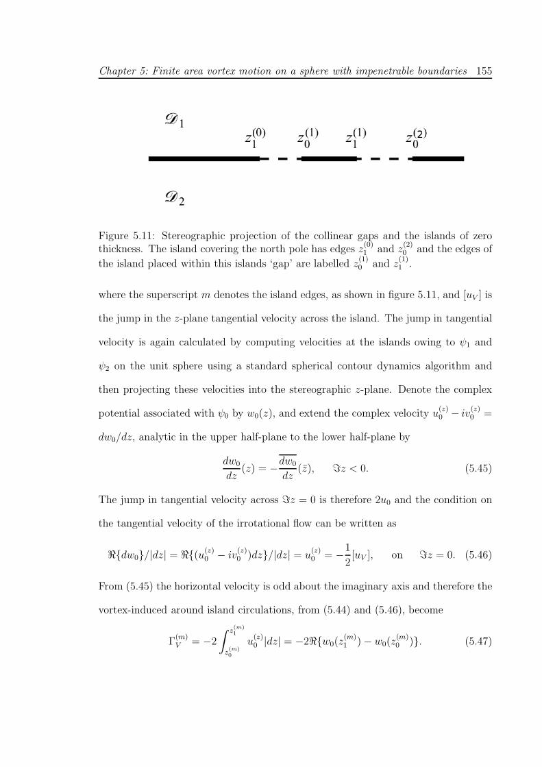
Chapter 5: Finite area vortex motion on a sphere with impenetrable boundaries 155
Figure 5.11: Stereographic projection of the collinear gaps and the islands of zerothickness. The island covering the north pole has edges z
(0)1 and z
(2)0 and the edges of
the island placed within this islands ‘gap’ are labelled z(1)0 and z
(1)1 .
where the superscript m denotes the island edges, as shown in figure 5.11, and [uV ] is
the jump in the z-plane tangential velocity across the island. The jump in tangential
velocity is again calculated by computing velocities at the islands owing to ψ1 and
ψ2 on the unit sphere using a standard spherical contour dynamics algorithm and
then projecting these velocities into the stereographic z-plane. Denote the complex
potential associated with ψ0 by w0(z), and extend the complex velocity u(z)0 − iv
(z)0 =
dw0/dz, analytic in the upper half-plane to the lower half-plane by
dw0
dz(z) = −dw0
dz(z), ℑz < 0. (5.45)
The jump in tangential velocity across ℑz = 0 is therefore 2u0 and the condition on
the tangential velocity of the irrotational flow can be written as
ℜdw0/|dz| = ℜ(u(z)0 − iv
(z)0 )dz/|dz| = u
(z)0 = −1
2[uV ], on ℑz = 0. (5.46)
From (5.45) the horizontal velocity is odd about the imaginary axis and therefore the
vortex-induced around island circulations, from (5.44) and (5.46), become
Γ(m)V = −2
∫ z(m)1
z(m)0
u(z)0 |dz| = −2ℜw0(z
(m)1 ) − w0(z
(m)0 ). (5.47)
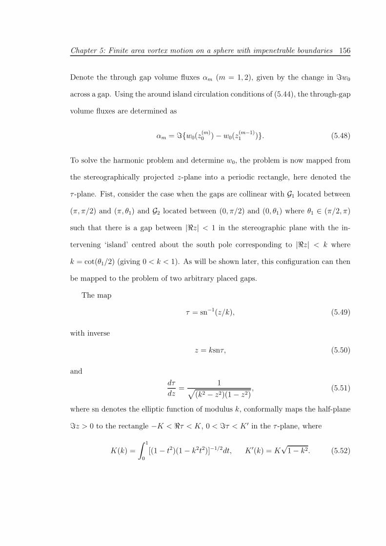
Chapter 5: Finite area vortex motion on a sphere with impenetrable boundaries 156
Denote the through gap volume fluxes αm (m = 1, 2), given by the change in ℑw0
across a gap. Using the around island circulation conditions of (5.44), the through-gap
volume fluxes are determined as
αm = ℑw0(z(m)0 ) − w0(z
(m−1)1 ). (5.48)
To solve the harmonic problem and determine w0, the problem is now mapped from
the stereographically projected z-plane into a periodic rectangle, here denoted the
τ -plane. Fist, consider the case when the gaps are collinear with G1 located between
(π, π/2) and (π, θ1) and G2 located between (0, π/2) and (0, θ1) where θ1 ∈ (π/2, π)
such that there is a gap between |ℜz| < 1 in the stereographic plane with the in-
tervening ‘island’ centred about the south pole corresponding to |ℜz| < k where
k = cot(θ1/2) (giving 0 < k < 1). As will be shown later, this configuration can then
be mapped to the problem of two arbitrary placed gaps.
The map
τ = sn−1(z/k), (5.49)
with inverse
z = ksnτ, (5.50)
and
dτ
dz=
1√
(k2 − z2)(1 − z2), (5.51)
where sn denotes the elliptic function of modulus k, conformally maps the half-plane
ℑz > 0 to the rectangle −K < ℜτ < K, 0 < ℑτ < K ′ in the τ -plane, where
K(k) =
∫ 1
0
[(1 − t2)(1 − k2t2)]−1/2dt, K ′(k) = K√
1 − k2. (5.52)
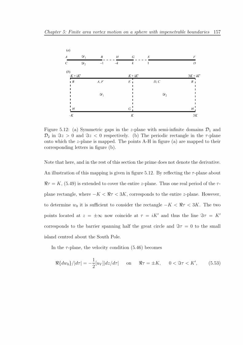
Chapter 5: Finite area vortex motion on a sphere with impenetrable boundaries 157
Figure 5.12: (a) Symmetric gaps in the z-plane with semi-infinite domains D1 andD2 in ℑz > 0 and ℑz < 0 respectively. (b) The periodic rectangle in the τ -planeonto which the z-plane is mapped. The points A-H in figure (a) are mapped to theircorresponding letters in figure (b).
Note that here, and in the rest of this section the prime does not denote the derivative.
An illustration of this mapping is given in figure 5.12. By reflecting the τ -plane about
ℜτ = K, (5.49) is extended to cover the entire z-plane. Thus one real period of the τ -
plane rectangle, where −K < ℜτ < 3K, corresponds to the entire z-plane. However,
to determine w0 it is sufficient to consider the rectangle −K < ℜτ < 3K. The two
points located at z = ±∞ now coincide at τ = iK ′ and thus the line ℑτ = K ′
corresponds to the barrier spanning half the great circle and ℑτ = 0 to the small
island centred about the South Pole.
In the τ -plane, the velocity condition (5.46) becomes
ℜdw0/|dτ | = −1
2[uV ]|dz/dτ | on ℜτ = ±K, 0 < ℑτ < K ′, (5.53)
Chapter 5: Finite area vortex motion on a sphere with impenetrable boundaries 158
and (5.48), the through gap flux conditions, become
ℑw0 = α1 = α on ℑτ = 0, |ℜτ | < K,
ℑw0 = α2 = 0 on ℑτ = K ′, |ℜτ | < K.
(5.54)
This condition is satisfied by a uniform stream in the ℜτ -direction such that the
tangential velocity condition (5.53) is not effected. Thus
w0 = α(K ′ − τ)/K ′ + w00, (5.55)
where w00 is the complex potential of an irrotational flow. A suitable expression for
w00 can be obtained through a further mapping of the τ -plane rectangle to the upper
half of an annulus δ1 < |σ| < δ2 in the complex σ-plane. This mapping is given by
σ = exp(πτ/K ′), (5.56)
such that
δ2,1 = exp(±πK/K ′). (5.57)
The complex potential w00 then satisfies
ℑw00 = 0 on φ = 0, π, δ1 < |σ| < δ2,
ℜdw00/|dσ| = −1
2[uV ]|dz/dσ| on |σ| = δ1,2, 0 < φ < π,
(5.58)
where φ = arg σ. Within the annulus w00 is harmonic and can thus be written as
w00 =∑′
anσn, (5.59)
where n ∈ Z and the prime indicates that the n = 0 term is omitted. Along with
the n = 0 term the allowable log σ term is also omitted from (5.59). Both these
Chapter 5: Finite area vortex motion on a sphere with impenetrable boundaries 159
terms have been absorbed into the constant α in (5.55) and are thus absent in (5.59).
Further, since w00 can be extended in to the lower half of the σ-plane through
w00(σ) = w00(σ), (5.60)
the an in (5.59) can be taken as real. On the σ-domain boundaries, |σ| = δ1,2,
dσ/|dσ| = ieiφ and thus (5.58) gives
ℜdw00/|dσ| =∑
′nanℜσn−1ieiφ =
∞∑
1
b(1,2)n sinnφ, (5.61)
where
b(1,2)n = − n
δ1,2
(anδn1,2 + δ−nδ
−n1,2 ), n ∈ Z
+. (5.62)
The b(1,2)n are the Fourier Sine coefficients in the expansion of −1
2[uV ]|dz/dσ| on |σ| =
δ1,2, 0 < φ < π and are given explicitly by
b(1,2)n = − K ′
2π2δ1,2
∫ π
0
[uV ](
(k2 − z21,2)(1 − z2
1,2))
12 sin(nφ)dφ, (5.63)
where, using the mappings (5.50) and (5.56)
z2,1 = ksn
[
K ′
πlog σ
]
= ksn
[
±K + iK ′φ
π
]
, (5.64)
which correspond to purely real points lying within the gaps. The coefficients bn can
now be determined numerically using discrete fast Fourier transforms evaluating the
integral in (5.63) at points spaced evenly in φ. The coefficients an in (5.59) are given
by
an =δ2b
(2)|n|δ
−n1 − δ1b
(1)|n|δ
−n2
|n|(δn1 δ
−n2 − δn
2 δ−n1 )
, n = ±1,±2,±3, ... (5.65)
Finally, to determine the velocity field owing to w0 in the stereographic z-plane the
through-gap volume flux α must be determined. The island edges, given ny z = ±k
Chapter 5: Finite area vortex motion on a sphere with impenetrable boundaries 160
in the z-plane, correspond to τ = ±K and σ = δ1,2 giving
ℜw0|z=k − w0|z=−k = −2αK
K ′+∑
′an(δn2 − δn
1 ), (5.66)
where, again, n ∈ Z and the prime indicates that the n = 0 term is omitted. Thus,
(5.66) along with (5.47) and (5.48) give the through-gap volume flux
α =K ′
2K
[
1
2ΓV +
∞∑
1
δ1b(1)n + δ2b
(2)n
2
]
. (5.67)
Using (5.55), (5.59), (5.65) and (5.3) the complex potential of the required irrotational
velocity field w0 is hence determined. The irrotational velocity field owing to w0 in
the z-plane is then given by
u(z)0 − iv
(z)0 =
dw0
dσ
dσ
dτ
dτ
dz=
π
K ′
[
ασ/K ′ +∑
′nanσn
((k2 − z2)(1 − z2))12
]
, (5.68)
where σ = exp[(π/K ′)sn−1(z/k)]. These velocities are then projected back to the
sphere and added to those owing to ψ1 and ψ2 to give the total velocity field on the
surface of the sphere. Importantly, in this case the image of the vortex patch has been
explicitly included when determining the velocity fields owing to ψ1 and ψ2. Thus
the difference here to the examples previously considered is that when projecting
velocities back to the sphere the velocity field arising due to the Gauss constraint
(see (5.9)) is not added back on to the total velocity field. Points on the vortex
contour are then advected as detailed in section 5.1.
5.3.1 Background flows
Note that in the formulation presented above, the circulation around the island
is not necessarily zero, the circulation around the thin barrier extending to ∞ in the
Chapter 5: Finite area vortex motion on a sphere with impenetrable boundaries 161
z-plane will however be zero. Due to the topography of the sphere and the fact that
it is an enclosed surface an additional term is required to ensure net zero circulation.
In planar problems a vortex can initially be positioned at ‘infinity’ such that the
fluid surrounding the island is initially stagnant i.e. there is initially no circulation
about the island and owing to Kelvin’s Circulation theorem this will remain so for
all time. However, when considering the problems on the surface of the sphere such
an assumption cannot be made. Thus to ensure a net zero circulation around the
island in the spherical case it is required to place a point vortex of circulation −Γ in
the τ = sn−1(z/k) plane such that it maps to the centre of the island (i.e. the South
Pole in the symmetric gap case) in the z-plane. Label this point τ∞. Using equation
(3.6) of Johnson and McDonald (2005), the background complex potential required
to ensure zero circulation about the island is given by
wB =−Γ
2πilog
(
θ1[π(τ − τ∞)/4K]
θ1[π(τ − τ ′∞)/4K]
)
, (5.69)
where τ ′∞ is the reflection of τ∞ about the line τ = iK ′ i.e. τ ′∞ = τ∞ + 2(iK ′ −ℑτ∞).
The Hamiltonian associated with such background flows, required for the computation
of point vortex trajectories, is then given by
HB(τ, τ∞) = −Γℑ[wB]. (5.70)
Of course, this form of the complex potential is not restricted to imposing the net
zero circulation case and can be used to impose an additional circulation around an
object or a background flow due to fixed point vortices such as was done for a singly
connected case in section 5.2.2. The velocity field owing to such a background flow
Chapter 5: Finite area vortex motion on a sphere with impenetrable boundaries 162
in the z-plane is given by
u(z)B − iv
(z)B =
dwB
dτ
dτ
dz. (5.71)
Such velocity fields are added to (5.68) before projecting back to the sphere.
5.3.2 Point vortex trajectories
The vortex Hamiltonian for the planar analog of this problem is derived in Johnson
and McDonald (2005). The relationship between a Hamiltonian on the sphere Hs to
a Hamiltonian in the complex z-plane Hz is given by (Surana and Crowdy 2008)
Hs(φαi, θαi
) = Hz(zαi) +
1
4π
N∑
j=1
Γ2j log
1
(1 + z(αj)z(αj)), (5.72)
where αi denotes the position of the ith vortex in a pre-image ζ domain. For the
case of a single point vortex with circulation Γ1 = Γ located at z = zα1 and when the
two gaps in the barrier are collinear with G1 located between (π, π/2) and (π, θ1) and
G2 located between (0, π/2) and (0, θ1) where θ1 ∈ (π/2, π) such that the resulting
island centred about the south pole corresponds to |ℜz| < k where k = cot(θ1/2), the
vortex Hamiltonian is given by
Hs(z, z) =(Γ2/4π) log |(k2 − z2)1/2(1 − z2)1/2ϑ1[iπ(ℑsn−1(z/k) −K ′)/2K]|
+ (Γ2/4π) log |1/(1 + zz)| − Γℑ[wB],
(5.73)
where wB is given in (5.69) and here τ∞ = 0. Vortex trajectories (and also finite area
vortex motion) for the case when the island lies asymmetrically between the barrier
spanning half a great circle can be deduced through mapping to the symmetric case.
An island in the sterographically projected z-plane located between x0 < ℑz < x1
Chapter 5: Finite area vortex motion on a sphere with impenetrable boundaries 163
(with −1 < x0 < x1 < 1) within a gap corresponding to −1 < ℑz < 1 is mapped
back to the symmetric problem in the z-plane via the Mobius map given by
z = (−αz + 1)/(z − α), (5.74)
leaving the gap of width of 2 unchanged but moving the island to lie along |ℜz| ≤
k < 1 where
α = exp(cosh−1[(x0x1 +1)/(x0 +x1)]), k = exp(cosh−1[(x0x1−1)/(x0−x1)]). (5.75)
This mapping along with the transformation
H z(zα) = Hz(zα) + (Γ2/4π) log |dz/dz|zα, (5.76)
and equation (5.73) give the appropriate vortex Hamiltonian in the z-plane. Finally,
it is simplest to obtain the vortex Hamiltonian for the case when G1 and G2 are
located at arbitrary locations on the barrier by considering one of the islands to
be centred about the north pole and the other to be located arbitrarily along the
same great circle and then mapping to the case of two collinear gaps and applying
the appropriate transformation to the Hamiltonian (5.72). This corresponds to the
configuration in the Dz domain where the gap is located between −r < z < r (r ∈ R+)
with the island, whose edges are here denoted z(L1) and z(L2), contained within the
gap such that −r < z(L1) < z(L2) < r. The map taking the z-plane to the z plane
considered above is simply the contraction
z =z
r. (5.77)
The domain Dz is then mapped to the domain Dz such that the gaps are now collinear
using (5.74). Through a standard rotation on the surface of the sphere, the two islands
can be placed such that they lie along arbitrary sections of a great circle.
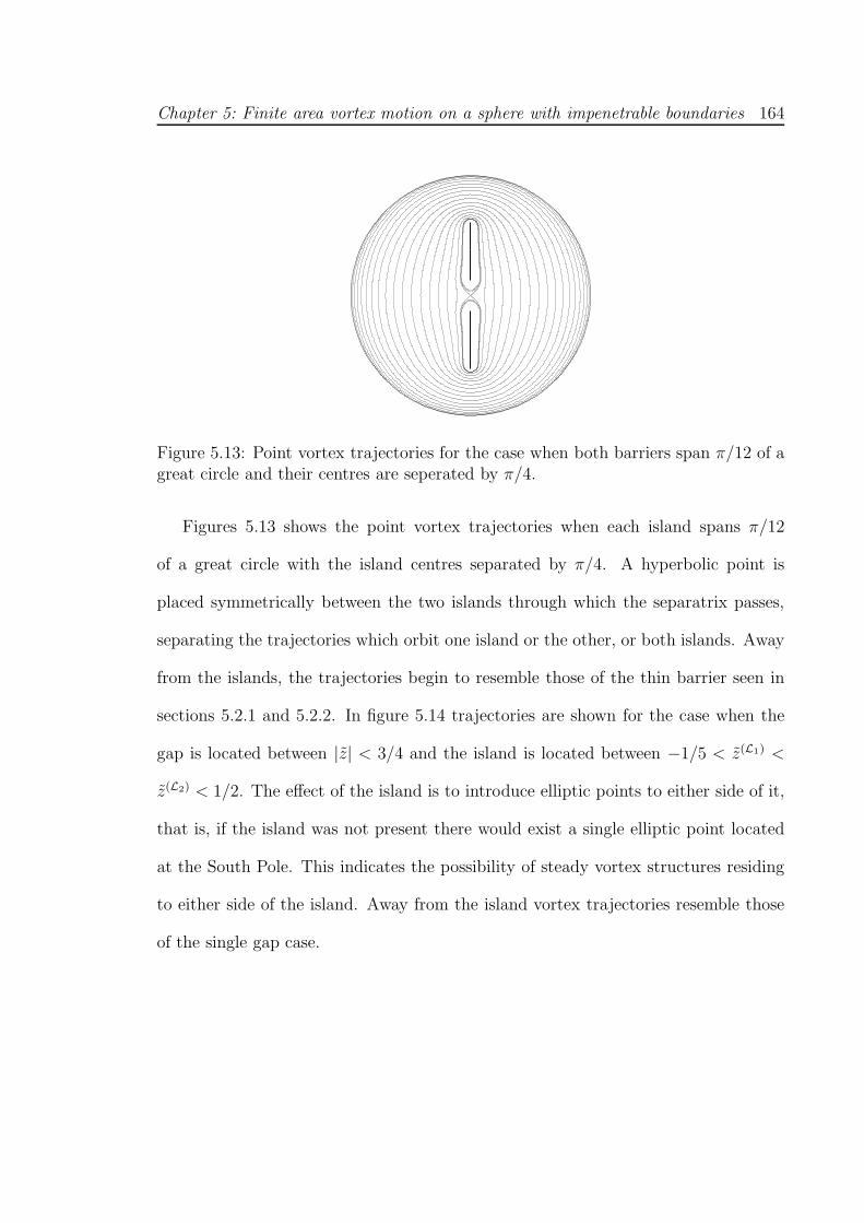
Chapter 5: Finite area vortex motion on a sphere with impenetrable boundaries 164
Figure 5.13: Point vortex trajectories for the case when both barriers span π/12 of agreat circle and their centres are seperated by π/4.
Figures 5.13 shows the point vortex trajectories when each island spans π/12
of a great circle with the island centres separated by π/4. A hyperbolic point is
placed symmetrically between the two islands through which the separatrix passes,
separating the trajectories which orbit one island or the other, or both islands. Away
from the islands, the trajectories begin to resemble those of the thin barrier seen in
sections 5.2.1 and 5.2.2. In figure 5.14 trajectories are shown for the case when the
gap is located between |z| < 3/4 and the island is located between −1/5 < z(L1) <
z(L2) < 1/2. The effect of the island is to introduce elliptic points to either side of it,
that is, if the island was not present there would exist a single elliptic point located
at the South Pole. This indicates the possibility of steady vortex structures residing
to either side of the island. Away from the island vortex trajectories resemble those
of the single gap case.
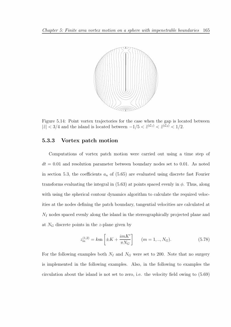
Chapter 5: Finite area vortex motion on a sphere with impenetrable boundaries 165
Figure 5.14: Point vortex trajectories for the case when the gap is located between|z| < 3/4 and the island is located between −1/5 < z(L1) < z(L2) < 1/2.
5.3.3 Vortex patch motion
Computations of vortex patch motion were carried out using a time step of
dt = 0.01 and resolution parameter between boundary nodes set to 0.01. As noted
in section 5.3, the coefficients an of (5.65) are evaluated using discrete fast Fourier
transforms evaluating the integral in (5.63) at points spaced evenly in φ. Thus, along
with using the spherical contour dynamics algorithm to calculate the required veloc-
ities at the nodes defining the patch boundary, tangential velocities are calculated at
NI nodes spaced evenly along the island in the stereographically projected plane and
at NG discrete points in the z-plane given by
z(1,2)m = ksn
[
±K +imK ′
πNG
]
(m = 1, .., NG). (5.78)
For the following examples both NI and NG were set to 200. Note that no surgery
is implemented in the following examples. Also, in the following to examples the
circulation about the island is not set to zero, i.e. the velocity field owing to (5.69)
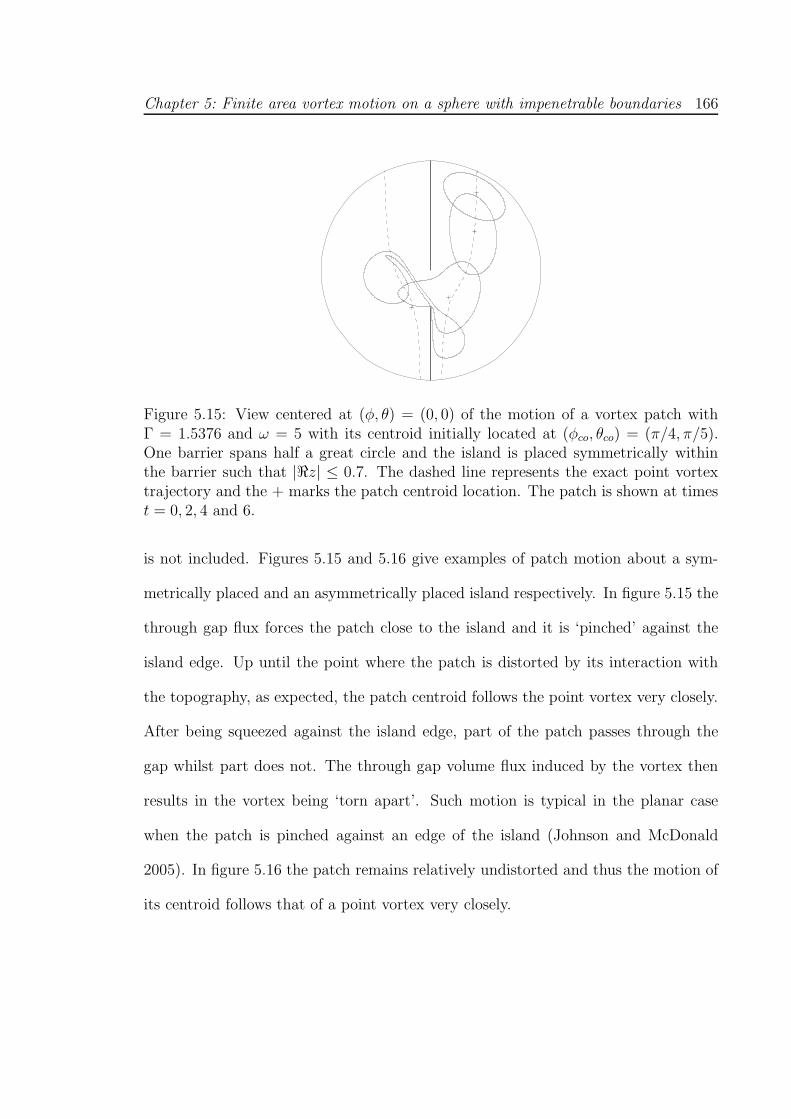
Chapter 5: Finite area vortex motion on a sphere with impenetrable boundaries 166
Figure 5.15: View centered at (φ, θ) = (0, 0) of the motion of a vortex patch withΓ = 1.5376 and ω = 5 with its centroid initially located at (φco, θco) = (π/4, π/5).One barrier spans half a great circle and the island is placed symmetrically withinthe barrier such that |ℜz| ≤ 0.7. The dashed line represents the exact point vortextrajectory and the + marks the patch centroid location. The patch is shown at timest = 0, 2, 4 and 6.
is not included. Figures 5.15 and 5.16 give examples of patch motion about a sym-
metrically placed and an asymmetrically placed island respectively. In figure 5.15 the
through gap flux forces the patch close to the island and it is ‘pinched’ against the
island edge. Up until the point where the patch is distorted by its interaction with
the topography, as expected, the patch centroid follows the point vortex very closely.
After being squeezed against the island edge, part of the patch passes through the
gap whilst part does not. The through gap volume flux induced by the vortex then
results in the vortex being ‘torn apart’. Such motion is typical in the planar case
when the patch is pinched against an edge of the island (Johnson and McDonald
2005). In figure 5.16 the patch remains relatively undistorted and thus the motion of
its centroid follows that of a point vortex very closely.
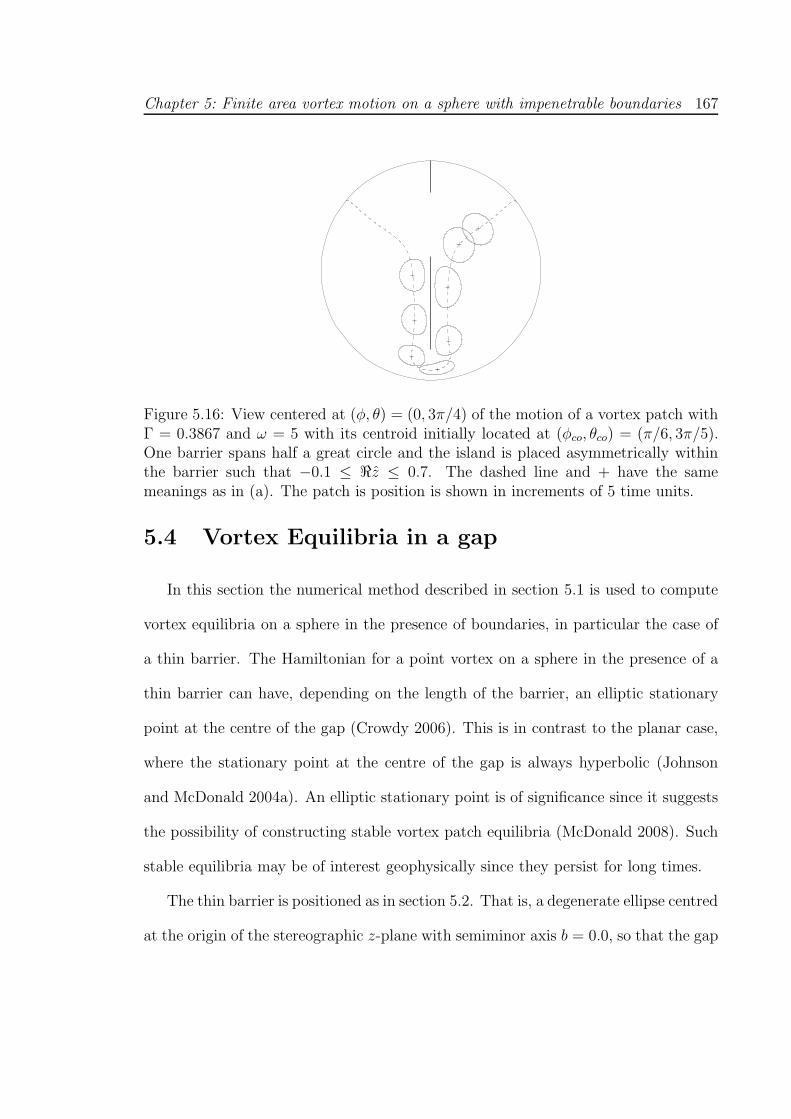
Chapter 5: Finite area vortex motion on a sphere with impenetrable boundaries 167
Figure 5.16: View centered at (φ, θ) = (0, 3π/4) of the motion of a vortex patch withΓ = 0.3867 and ω = 5 with its centroid initially located at (φco, θco) = (π/6, 3π/5).One barrier spans half a great circle and the island is placed asymmetrically withinthe barrier such that −0.1 ≤ ℜz ≤ 0.7. The dashed line and + have the samemeanings as in (a). The patch is position is shown in increments of 5 time units.
5.4 Vortex Equilibria in a gap
In this section the numerical method described in section 5.1 is used to compute
vortex equilibria on a sphere in the presence of boundaries, in particular the case of
a thin barrier. The Hamiltonian for a point vortex on a sphere in the presence of a
thin barrier can have, depending on the length of the barrier, an elliptic stationary
point at the centre of the gap (Crowdy 2006). This is in contrast to the planar case,
where the stationary point at the centre of the gap is always hyperbolic (Johnson
and McDonald 2004a). An elliptic stationary point is of significance since it suggests
the possibility of constructing stable vortex patch equilibria (McDonald 2008). Such
stable equilibria may be of interest geophysically since they persist for long times.
The thin barrier is positioned as in section 5.2. That is, a degenerate ellipse centred
at the origin of the stereographic z-plane with semiminor axis b = 0.0, so that the gap
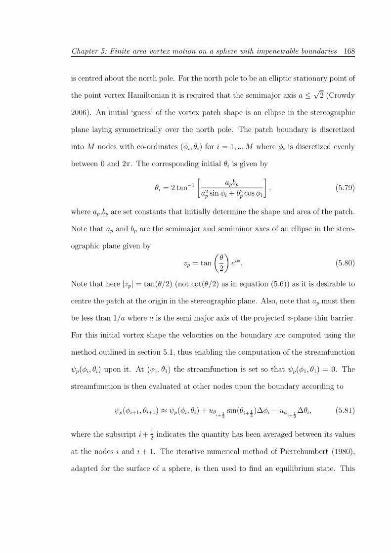
Chapter 5: Finite area vortex motion on a sphere with impenetrable boundaries 168
is centred about the north pole. For the north pole to be an elliptic stationary point of
the point vortex Hamiltonian it is required that the semimajor axis a ≤√
2 (Crowdy
2006). An initial ‘guess’ of the vortex patch shape is an ellipse in the stereographic
plane laying symmetrically over the north pole. The patch boundary is discretized
into M nodes with co-ordinates (φi, θi) for i = 1, ..,M where φi is discretized evenly
between 0 and 2π. The corresponding initial θi is given by
θi = 2 tan−1
[
apbpa2
p sin φi + b2p cos φi
]
, (5.79)
where ap,bp are set constants that initially determine the shape and area of the patch.
Note that ap and bp are the semimajor and semiminor axes of an ellipse in the stere-
ographic plane given by
zp = tan
(
θ
2
)
eiφ. (5.80)
Note that here |zp| = tan(θ/2) (not cot(θ/2) as in equation (5.6)) as it is desirable to
centre the patch at the origin in the stereographic plane. Also, note that ap must then
be less than 1/a where a is the semi major axis of the projected z-plane thin barrier.
For this initial vortex shape the velocities on the boundary are computed using the
method outlined in section 5.1, thus enabling the computation of the streamfunction
ψp(φi, θi) upon it. At (φ1, θ1) the streamfunction is set so that ψp(φ1, θ1) = 0. The
streamfunction is then evaluated at other nodes upon the boundary according to
ψp(φi+1, θi+1) ≈ ψp(φi, θi) + uθi+ 1
2
sin(θi+ 12)∆φi − uφ
i+ 12
∆θi, (5.81)
where the subscript i+ 12
indicates the quantity has been averaged between its values
at the nodes i and i + 1. The iterative numerical method of Pierrehumbert (1980),
adapted for the surface of a sphere, is then used to find an equilibrium state. This
Chapter 5: Finite area vortex motion on a sphere with impenetrable boundaries 169
involves fixing the position of nodes 1 and M/2 + 1 and holding φ constant at all
other nodes whilst iterating their θ location until the boundary becomes a stream-
line. Owing to the symmetry of the problem, here only the nodes 1 to M/2 + 1 are
considered, the location of remaining nodes, M/2 + 2 to M , are obtained through
reflection of the boundary about the gap, i.e. θM/2+2 = θM/2 and so forth. Figure
5.17 shows the initial set-up of the patch and nodes. Fixing φi and varying θTi by
δθi, where the superscript T has been introduced to indicate T th iteration of θi, the
streamfunction varies as
ψp(φi, θTi + δθi) ≈ ψp(φi, θ
Ti ) − uφi
δθi, (5.82)
and thus the new θi location θT+1i is given by
θT+1i = θT
i + kψp(φi, θ
Ti )
uφi
, (5.83)
where k is a relaxation parameter introduced to ensure numerical convergence (Pier-
rehumbert 1980). Following each iteration the area A and hence circulation of the
vortex patch is recalculated using (5.15). The Gauss constraint on the surface of the
sphere (i.e∫ ∫
ωsdS = 0) is embedded in the equations of contour dynamics. Thus
when the area of the vortex patch changes, here the vorticity jump, ω, is kept con-
stant and the vorticity of the patch, ω, must be modified appropriately. Following
each iteration the patch vorticity and circulation is given by
ω =ω
4π(4π −A), (5.84)
and
Γ = ωA. (5.85)
Chapter 5: Finite area vortex motion on a sphere with impenetrable boundaries 170
Once the streamfunction becomes constant on the boundary of the patch (to within
some numerical tolerance) a steady solution is realized. The patch area and circula-
tion computed at each iteration are also monitored for convergence. For the results
reported here vortex patches initially had ω = 1, a resolution of 0.01 between adjacent
nodes on the patch boundary was used and the number of nodes on the barrier was
set to N = 400. The relaxation parameter was set to k = 0.6. The fixed boundary
nodes were set as
(φ1, θ1) =
(
π
2, 2 tan−1
[
apbpa2
p sin π/2 + b2p cosπ/2
])
(5.86)
and
(φM/2+1, θM/2+1) =
(
3π
2, 2 tan−1
[
apbpa2
p sin 3π/2 + b2p cos 3π/2
])
. (5.87)
Convergence was generally realized within 50 iterations. Figures 5.18(a) and 5.18(b)
show the family of vortex equilibria for the case where the gap-width a = 1.0 in the
stereographic z-plane and on the sphere respectively. The patches were initially set
with ap = 0.2 in all cases and bp = 0.2, 0.4, 0.6, 1.0, 1.4 and 2.0 then iterated to the
steady states observed in the figures. Figures 5.19(a) and 5.19(b) show the family of
equilibria when a = 1.4 for the same initial patch configurations as figures 5.18(a)
and 5.18(b).
The robustness of the computed equilibria was examined by using them as initial
conditions in a time-dependent simulation using the algorithm detailed in section
5.1. Since there are inevitably small numerical errors inherent in the algorithm,
unstable equilibria would be expected to diverge from their steady position within
time, whereas stable equilibria would be expected to remain close to their equilibrium
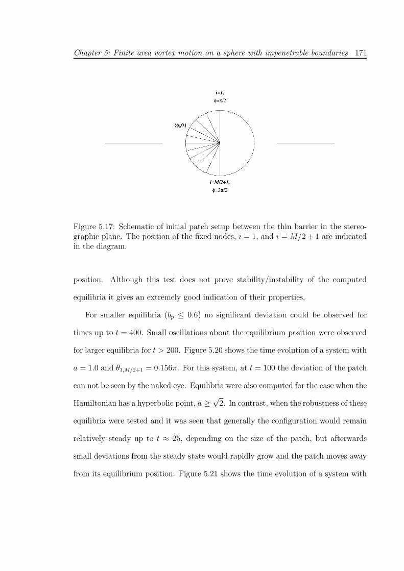
Chapter 5: Finite area vortex motion on a sphere with impenetrable boundaries 171
Figure 5.17: Schematic of initial patch setup between the thin barrier in the stereo-graphic plane. The position of the fixed nodes, i = 1, and i = M/2 + 1 are indicatedin the diagram.
position. Although this test does not prove stability/instability of the computed
equilibria it gives an extremely good indication of their properties.
For smaller equilibria (bp ≤ 0.6) no significant deviation could be observed for
times up to t = 400. Small oscillations about the equilibrium position were observed
for larger equilibria for t > 200. Figure 5.20 shows the time evolution of a system with
a = 1.0 and θ1,M/2+1 = 0.156π. For this system, at t = 100 the deviation of the patch
can not be seen by the naked eye. Equilibria were also computed for the case when the
Hamiltonian has a hyperbolic point, a ≥√
2. In contrast, when the robustness of these
equilibria were tested and it was seen that generally the configuration would remain
relatively steady up to t ≈ 25, depending on the size of the patch, but afterwards
small deviations from the steady state would rapidly grow and the patch moves away
from its equilibrium position. Figure 5.21 shows the time evolution of a system with
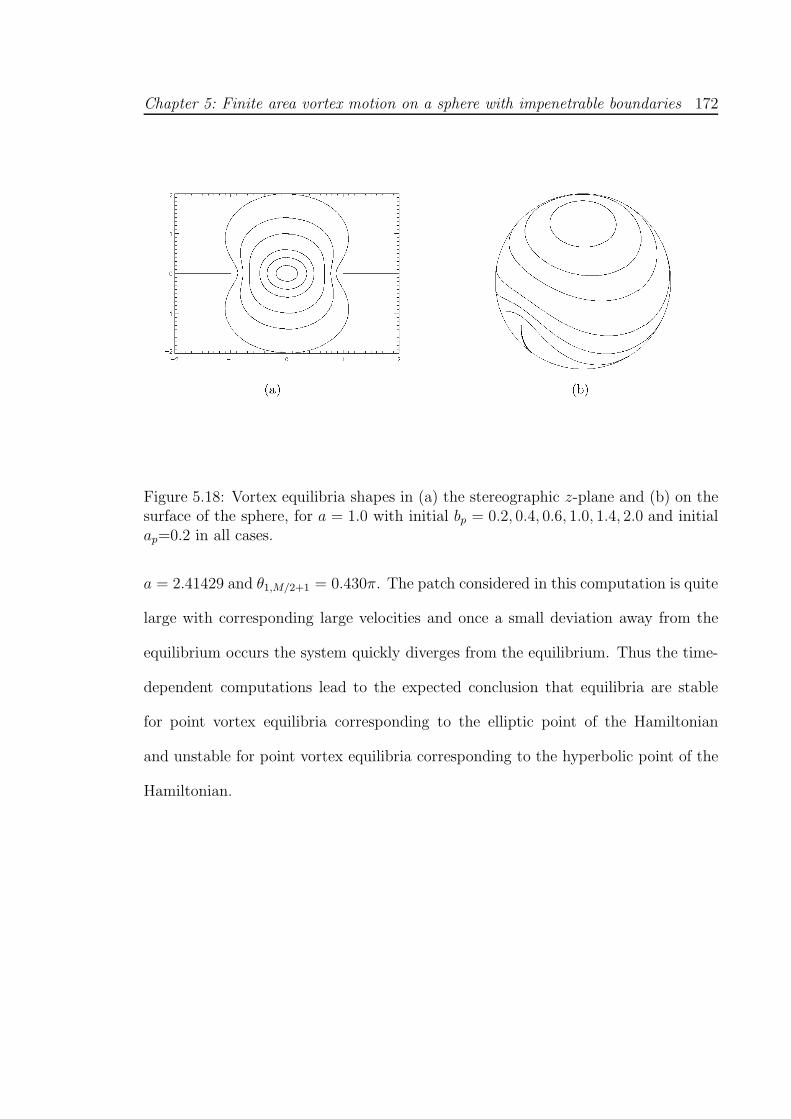
Chapter 5: Finite area vortex motion on a sphere with impenetrable boundaries 172
Figure 5.18: Vortex equilibria shapes in (a) the stereographic z-plane and (b) on thesurface of the sphere, for a = 1.0 with initial bp = 0.2, 0.4, 0.6, 1.0, 1.4, 2.0 and initialap=0.2 in all cases.
a = 2.41429 and θ1,M/2+1 = 0.430π. The patch considered in this computation is quite
large with corresponding large velocities and once a small deviation away from the
equilibrium occurs the system quickly diverges from the equilibrium. Thus the time-
dependent computations lead to the expected conclusion that equilibria are stable
for point vortex equilibria corresponding to the elliptic point of the Hamiltonian
and unstable for point vortex equilibria corresponding to the hyperbolic point of the
Hamiltonian.
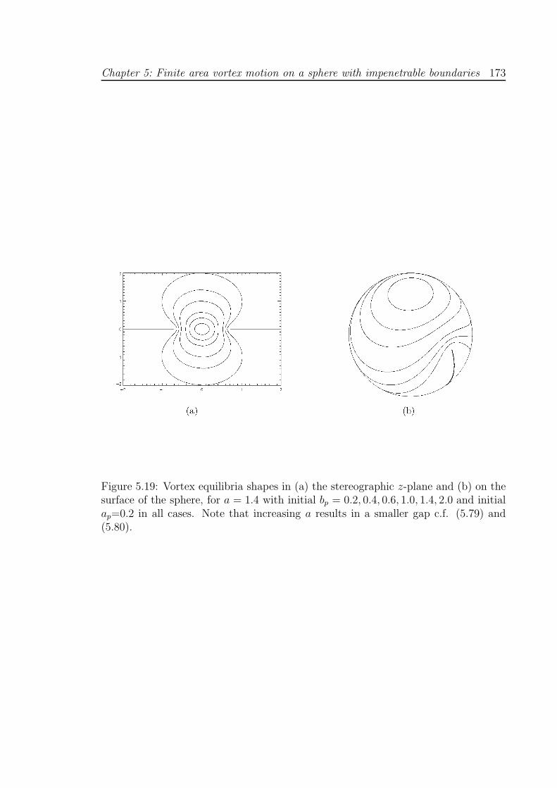
Chapter 5: Finite area vortex motion on a sphere with impenetrable boundaries 173
Figure 5.19: Vortex equilibria shapes in (a) the stereographic z-plane and (b) on thesurface of the sphere, for a = 1.4 with initial bp = 0.2, 0.4, 0.6, 1.0, 1.4, 2.0 and initialap=0.2 in all cases. Note that increasing a results in a smaller gap c.f. (5.79) and(5.80).
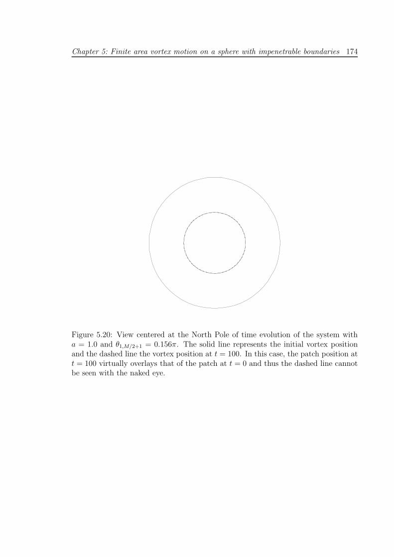
Chapter 5: Finite area vortex motion on a sphere with impenetrable boundaries 174
Figure 5.20: View centered at the North Pole of time evolution of the system witha = 1.0 and θ1,M/2+1 = 0.156π. The solid line represents the initial vortex positionand the dashed line the vortex position at t = 100. In this case, the patch position att = 100 virtually overlays that of the patch at t = 0 and thus the dashed line cannotbe seen with the naked eye.
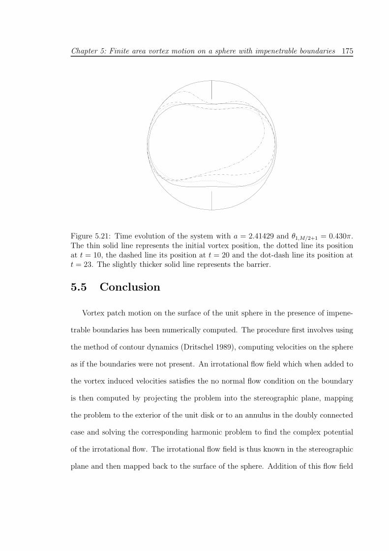
Chapter 5: Finite area vortex motion on a sphere with impenetrable boundaries 175
Figure 5.21: Time evolution of the system with a = 2.41429 and θ1,M/2+1 = 0.430π.The thin solid line represents the initial vortex position, the dotted line its positionat t = 10, the dashed line its position at t = 20 and the dot-dash line its position att = 23. The slightly thicker solid line represents the barrier.
5.5 Conclusion
Vortex patch motion on the surface of the unit sphere in the presence of impene-
trable boundaries has been numerically computed. The procedure first involves using
the method of contour dynamics (Dritschel 1989), computing velocities on the sphere
as if the boundaries were not present. An irrotational flow field which when added to
the vortex induced velocities satisfies the no normal flow condition on the boundary
is then computed by projecting the problem into the stereographic plane, mapping
the problem to the exterior of the unit disk or to an annulus in the doubly connected
case and solving the corresponding harmonic problem to find the complex potential
of the irrotational flow. The irrotational flow field is thus known in the stereographic
plane and then mapped back to the surface of the sphere. Addition of this flow field
Chapter 5: Finite area vortex motion on a sphere with impenetrable boundaries 176
to that given by the contour dynamics algorithm in the absence of boundaries gives
the appropriate flow field for the boundaries being present and hence the resulting
vortex patch motion on the surface of the sphere can be computed.
Singly-connected domains considered here included an ellipse in the projected z-
plane, a longitudinal wedge and a half-longitudinal wedge. Patch trajectories about a
thin barrier with a gap were computed with and without the presence of a background
flow. Background flows caused by a dipole fixed in the centre of the barrier and for
point vortices fixed at the equator were considered.
In cases in which the patch remained close to circular the path of the patch centroid
followed that of the corresponding point vortex trajectory very closely even with the
presence of a background flow. When the path of the centroid travelled within close
proximity to the barrier’s edge, deformation of the patch occurred often resulting in
filamentation. Despite this, centroid paths still showed good agreement with exact
point vortex solutions. Exceptions to this can be found when a background flow
parallel to a “long barrier” in the vicinity of the gap is present, where a sufficiently
strong background flow could result in a patch being “squeezed” against the barriers
edge resulting in the vortex splitting. Such splitting occasionally resulted in a quasi-
steady vortex being “trapped” against the barrier’s edge.
Patch centroid motion in domains including the longitudinal and half-longitudinal
wedge again demonstrated very good agreement with the corresponding point vortex
motion. Minor filamentation could be observed in such domains in cases in which
the patch is deformed when passing around an edge of the wedge or when the patch
travels within close proximity of the boundary for some time, resulting from the shear
Chapter 5: Finite area vortex motion on a sphere with impenetrable boundaries 177
flow due to the “image” vorticity and the curvature of the sphere.
The doubly connected case of a thin barrier with two gaps was also considered.
Good agreement is again seen between the motion of point vortices and patches which
undergo little distortion. Behaviour typical to that seen in the planar case is seen
resulting from the through gap fluxes generated by the vortex. New features, such
as elliptic points of the Hamiltonian residing to either side of the island, are also
observed.
This method can also be applied to other doubly connected domains, indeed, the
method can in principle be applied to any domain for which a conformal mapping to
an annulus exists. It is also in principle possible to apply the method to domains of
higher connectivity by mapping to the unit disk with smaller circular disks excised
and solving the corresponding Dirichlet problem to obtain the appropriate irrotational
flow.
Vortex equilibria lying between the gap in the case of a “short barrier” were then
computed. It was shown that a family of equilibria exist for each gap width. Such
equilibria were shown to be stable by examining their robustness in a time-dependent
code. Such stable equilibria do not exist in the corresponding planar case as the point
vortex equilibrium midway between the gap corresponds to a hyperbolic point of the
Hamiltonian for all gap widths.
Chapter 6
Vortex motion in periodic domains
with impenetrable boundaries
Methods described in chapter 5 can also be adapted to compute the motion of finite
area vortices in singly periodic domains with boundaries i.e. vortex motion on the
surface of an infinite circular cylinder. The motion of vortices in periodic domains
is of interest from both an atmospheric and oceanic perspective, for example, the
Southern Ocean is an example of a periodic channel. Thus a periodic domain with
boundaries, such as that later considered in section 6.3, could be thought of as a
‘crude’ model of the Southern Ocean. The steps presented here for computing the
motion of vortices in periodic domains with boundaries are similar to those presented
in chapter 5.1, the main difference being that the unbounded cylindrical contour
dynamics algorithm described in appendix A is now used to compute the velocity
field on the boundary. Similar to the previous chapter, an irrotational velocity field
is sought such that, when added to the velocity field owing to the ‘unbounded’ vortex
178
Chapter 6: Vortex motion in periodic domains with impenetrable boundaries 179
generated flow, satisfies the no-normal flow condition on the boundary. The required
irrotational flow is obtained through mapping the harmonic problem from the cylinder
to a domain exterior to the unit circle and solving the resulting harmonic problem
in this simpler domain. In this chapter, two examples will be considered. First, the
case of a horizontal thin island in a periodic domain and second, a vertical semi-
infinite barrier. In both cases numerically computed finite area patch motion will be
compared to exact point vortex trajectories.
6.1 Problem formulation
The system consists of a shallow layer of constant depth, incompressible and
inviscid fluid in a simply connected domain D on the surface of the unit cylinder
(that is a 2π-periodic domain). Let Ψ denote the total streamfunction due to a finite
number of vortices (with piecewise constant vorticity) in the domain D such that the
no-normal flow boundary condition
Ψ = 0 on ∂D, (6.1)
is satisfied. Further, let ψ1 be the streamfunction owing to the vortices in the absence
of boundaries ∂D, which gives
dφ
dt= −∂ψ1
∂z,
dz
dt=∂ψ1
∂φ, (6.2)
where φ ∈ [0, 2π] is the azimuthal angle and z is the vertical coordinate. Velocities
on ∂D owing to ψ1 are computed using an unbounded cylindrical contour dynamics
algorithm (Dritschel 1989, and Appendix A.2). Now, introduce an irrotational flow,
Chapter 6: Vortex motion in periodic domains with impenetrable boundaries 180
with streamfunction ψ0, defined throughout D such that
Ψ = ψ1 + ψ0. (6.3)
The no-normal-flow condition on the boundary ∂D requires that
d(ψ1 + ψ0)|∂D = 0. (6.4)
Now, for ease of notation, let the azimuthal and vertical velocity fields owing to ψ1
and ψ0 be written as (u0, v0) and (u0, v0) respectively. Also, denote the periodic
domain Dz in which the complex coordinate z = φ + iz. Requiring that the total
normal component of the velocity field owing to ψ1 + ψ0 vanishes on ∂D gives the
relation
ℑ[(u0 − iv0)dz]∂Dz= −ℑ[(u0 − iv0)dz]∂Dz
. (6.5)
The steps in determining (u0, v0) now mirror those detailed in chapter 5.1. On the
unit circle in the ζ-plane (ζ = exp(iσ), 0 ≤ σ < 2π), noting that dw = (uφ − ivz)dz,
(6.5) can be written as
ℑ[
dw
dσ
]
∂Dζ
= −ℑ[
iζ
F ′(z)(u0 − iv0)
]
∂Dζ
= g(σ), (6.6)
where g(σ) is a known function on ∂Dζ , w is the complex potential associated with
the streamfunction ψ0 and F (z) is the mapping from Dz to the domain exterior to the
unit circle Dζ. Similar to chapter 5.1, the complex potential w can again be written
as (5.12), that is
w = iC log ζ +
∞∑
k=1
akζ−k (6.7)
where C ∈ R and determines the circulation around the boundary ∂Dz and the ak
are complex constants. Expressing g(σ) as a Fourier series, ak can be determined
Chapter 6: Vortex motion in periodic domains with impenetrable boundaries 181
efficiently by Fast Fourier Transforms. The velocity field owing to ψ0 in D is thus
given by
u0 − iv0 =
[
iC
ζ+
∞∑
k=1
−kakζ−k−1
]
F ′(z). (6.8)
To advect the vortex in the periodic domain, (6.8) is added to the velocity field
owing to ψ1 (calculated using an unbounded cylindrical contour dynamics algorithm
at discrete points on the contour defining the vortex patch) and time integration is
carried out using a fourth order Runge-Kutta method. Nodes on the patch boundary
are redistributed at the beginning of each time-step and the procedure presented
above repeated. In practice, the sum in (6.8) is truncated at some k = N .
6.2 Periodic thin islands
Consider a horizontal thin island of length r centred at the middle of a periodic
domain of period L. The series of mappings given by
ζ1(ζ) =rI
2
(
1
ζ+ ζ
)
, (6.9)
ζ2(ζ1) =iζ1 − 1
iζ1 + 1, (6.10)
z(ζ2) =L
2πilog ζ2, (6.11)
where rI is related implicitly to r through
r = L
[
1 − 1
πtan−1
(
2rI
r2I − 1
)]
, (6.12)
Chapter 6: Vortex motion in periodic domains with impenetrable boundaries 182
maps the exterior of the unit ζ-circle to the periodic z-domain exterior to a horizontal
thin island of length r centred in the periodic domain. It is useful to note that when
rI = 1, r = L/2 i.e. the thin barrier spans exactly half of the periodic domain. Also,
as rI → ∞, r → L, that is, the case of a period array of vortices above an infinite
solid wall is recovered. The first of these maps, (6.9), takes the exterior of the unit
ζ2-circle to the exterior of a thin island between −rI ≤ ζ1 ≤ rI . The second map
takes this thin island to an arc on the unit circle between φ < arg ζ2 < 2π − φ where
φ = tan−1
(
2rI
r2I − 1
)
, (6.13)
and finally, (6.11) takes this arc to a horizontal thin island between (L− r)/2 < z <
(L + r)/2 in the periodic strip. The branch cut in (6.11) is taken to be along the
positive real axis in Dζ2. The composition of these three maps can be written as
z(ζ) =L
2πilog
(
irI(1 + ζ2) − 2ζ
irI(1 + ζ2) + 2ζ
)
. (6.14)
Thus, the derivative of the map required for computing vortex patch trajectories is
given by
zζ =1
F ′(z)=
L
2πi
[
2irIζ − 2
irI(1 + ζ2) − 2ζ− 2irIζ + 2
irI(1 + ζ2) + 2ζ
]
(6.15)
Point vortex trajectories in the periodic z-domain are derived by considering the
vortex Hamiltonian in the unit circle and performing the appropriate transformation.
For the mapping into the periodic domain the standard transformation rule for the
Hamiltonian can be used as all the information about the images of vortices in the
periodic domain are encoded in the transform. This can be verified by mapping the
problem of a single vortex within the unit disk to a row of periodic vortices located
near a horizontal barrier. It can be shown that the velocity field at a vortex obtained
Chapter 6: Vortex motion in periodic domains with impenetrable boundaries 183
through the mapping is identical to that of the double vortex street considered in
Acheson (1990). The vortex Hamiltonian for a single vortex at position α in the unit
circle ρ-domain is given by
H(ρ)(α, α) =Γ2
4πlog(1 − αα). (6.16)
The map from the interior of the unit circle to the periodic z-domain exterior to
a horizontal thin island is also given by (6.14) (with ρ now replacing ζ) and thus
the derivative required in the transformation (5.76) is given by (6.15) (with ρ again
replacing ζ). Additionally, the map (6.11) has two logarithmic singularities within
the unit ζ-circle located at
ρ = ± i
rI
(
√
1 + r2I − 1
)
= ±is. (6.17)
Inserting (6.17) into (6.11) shows that these two points map to ℑz = ±∞ in Dz. For
the case when the circulation about the island in the domain Dz is zero it is therefore
necessary to impose an additional background flow by placing two point vortices, each
of circulation −Γ/2, at the points ρ = ±is. The complex potential associated a point
vortex of unit circulation located at η0 in the upper-half η = x+ iy plane is given by
W (η) = − i
2πlog
[
η − η0
η − η0
]
. (6.18)
This, along with the map from the interior of the unit circle to the upper half η-plane
given by
η = i1 − ρ
1 + ρ, (6.19)
results in a contribution to the Hamiltonian for the background flow due to vortices
of strength −Γ/2 and Γ/2 at ρ = ±is given by
Ψ(α, α) = ΓℑW =Γ2
4πlog
∣
∣
∣
∣
α2 + s2
1 + α2s2
∣
∣
∣
∣
. (6.20)
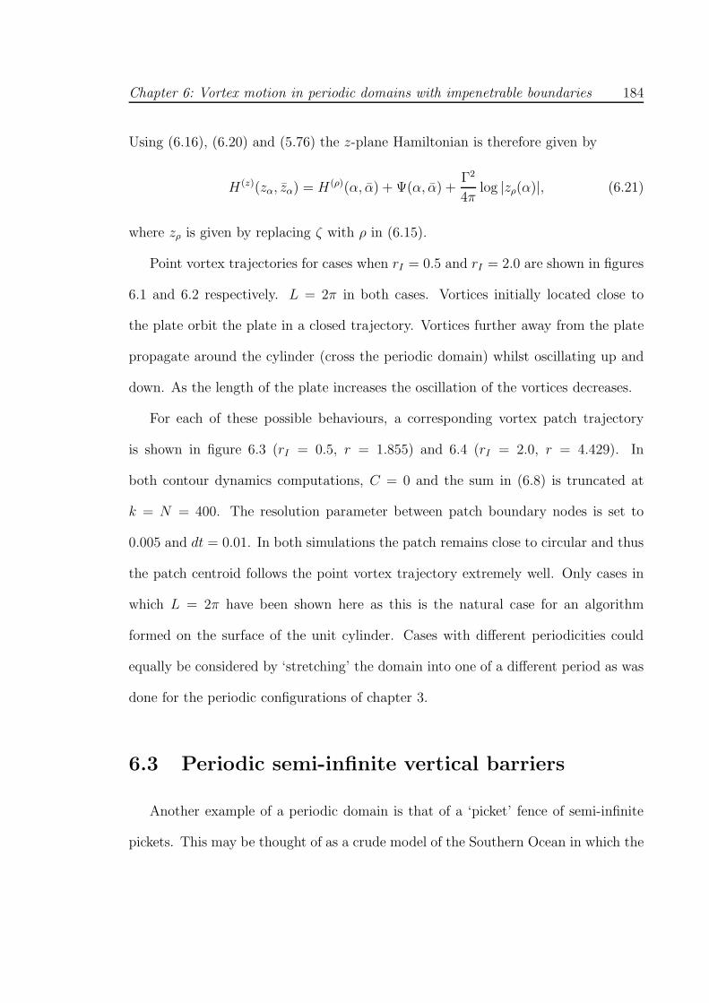
Chapter 6: Vortex motion in periodic domains with impenetrable boundaries 184
Using (6.16), (6.20) and (5.76) the z-plane Hamiltonian is therefore given by
H(z)(zα, zα) = H(ρ)(α, α) + Ψ(α, α) +Γ2
4πlog |zρ(α)|, (6.21)
where zρ is given by replacing ζ with ρ in (6.15).
Point vortex trajectories for cases when rI = 0.5 and rI = 2.0 are shown in figures
6.1 and 6.2 respectively. L = 2π in both cases. Vortices initially located close to
the plate orbit the plate in a closed trajectory. Vortices further away from the plate
propagate around the cylinder (cross the periodic domain) whilst oscillating up and
down. As the length of the plate increases the oscillation of the vortices decreases.
For each of these possible behaviours, a corresponding vortex patch trajectory
is shown in figure 6.3 (rI = 0.5, r = 1.855) and 6.4 (rI = 2.0, r = 4.429). In
both contour dynamics computations, C = 0 and the sum in (6.8) is truncated at
k = N = 400. The resolution parameter between patch boundary nodes is set to
0.005 and dt = 0.01. In both simulations the patch remains close to circular and thus
the patch centroid follows the point vortex trajectory extremely well. Only cases in
which L = 2π have been shown here as this is the natural case for an algorithm
formed on the surface of the unit cylinder. Cases with different periodicities could
equally be considered by ‘stretching’ the domain into one of a different period as was
done for the periodic configurations of chapter 3.
6.3 Periodic semi-infinite vertical barriers
Another example of a periodic domain is that of a ‘picket’ fence of semi-infinite
pickets. This may be thought of as a crude model of the Southern Ocean in which the
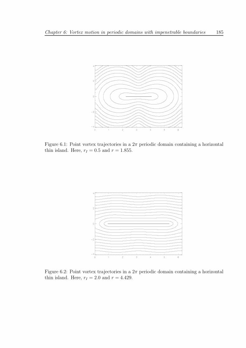
Chapter 6: Vortex motion in periodic domains with impenetrable boundaries 185
Figure 6.1: Point vortex trajectories in a 2π periodic domain containing a horizontalthin island. Here, rI = 0.5 and r = 1.855.
Figure 6.2: Point vortex trajectories in a 2π periodic domain containing a horizontalthin island. Here, rI = 2.0 and r = 4.429.
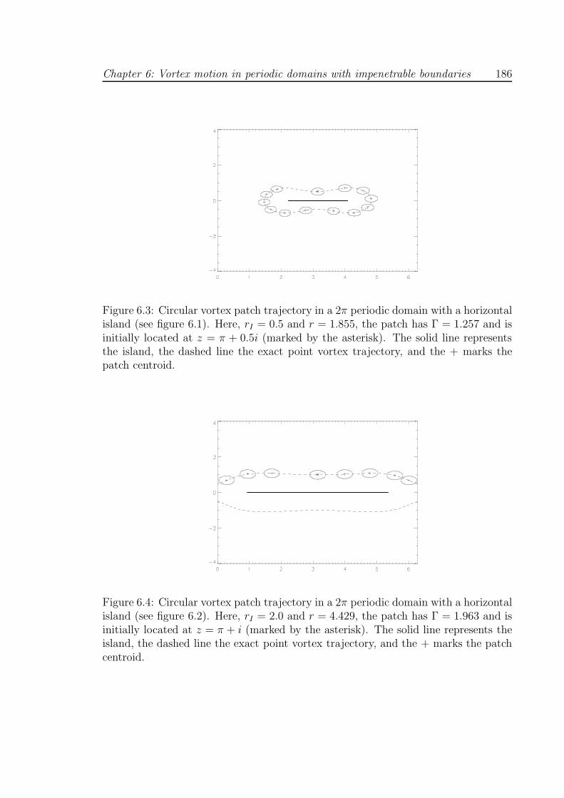
Chapter 6: Vortex motion in periodic domains with impenetrable boundaries 186
Figure 6.3: Circular vortex patch trajectory in a 2π periodic domain with a horizontalisland (see figure 6.1). Here, rI = 0.5 and r = 1.855, the patch has Γ = 1.257 and isinitially located at z = π + 0.5i (marked by the asterisk). The solid line representsthe island, the dashed line the exact point vortex trajectory, and the + marks thepatch centroid.
Figure 6.4: Circular vortex patch trajectory in a 2π periodic domain with a horizontalisland (see figure 6.2). Here, rI = 2.0 and r = 4.429, the patch has Γ = 1.963 and isinitially located at z = π + i (marked by the asterisk). The solid line represents theisland, the dashed line the exact point vortex trajectory, and the + marks the patchcentroid.
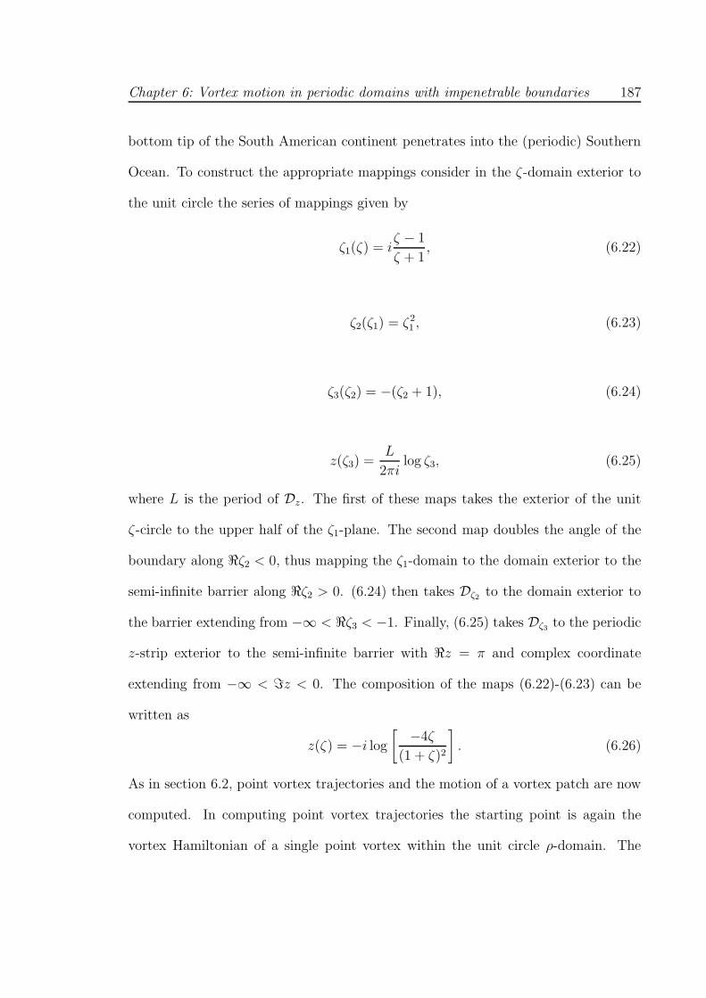
Chapter 6: Vortex motion in periodic domains with impenetrable boundaries 187
bottom tip of the South American continent penetrates into the (periodic) Southern
Ocean. To construct the appropriate mappings consider in the ζ-domain exterior to
the unit circle the series of mappings given by
ζ1(ζ) = iζ − 1
ζ + 1, (6.22)
ζ2(ζ1) = ζ21 , (6.23)
ζ3(ζ2) = −(ζ2 + 1), (6.24)
z(ζ3) =L
2πilog ζ3, (6.25)
where L is the period of Dz. The first of these maps takes the exterior of the unit
ζ-circle to the upper half of the ζ1-plane. The second map doubles the angle of the
boundary along ℜζ2 < 0, thus mapping the ζ1-domain to the domain exterior to the
semi-infinite barrier along ℜζ2 > 0. (6.24) then takes Dζ2 to the domain exterior to
the barrier extending from −∞ < ℜζ3 < −1. Finally, (6.25) takes Dζ3 to the periodic
z-strip exterior to the semi-infinite barrier with ℜz = π and complex coordinate
extending from −∞ < ℑz < 0. The composition of the maps (6.22)-(6.23) can be
written as
z(ζ) = −i log
[ −4ζ
(1 + ζ)2
]
. (6.26)
As in section 6.2, point vortex trajectories and the motion of a vortex patch are now
computed. In computing point vortex trajectories the starting point is again the
vortex Hamiltonian of a single point vortex within the unit circle ρ-domain. The
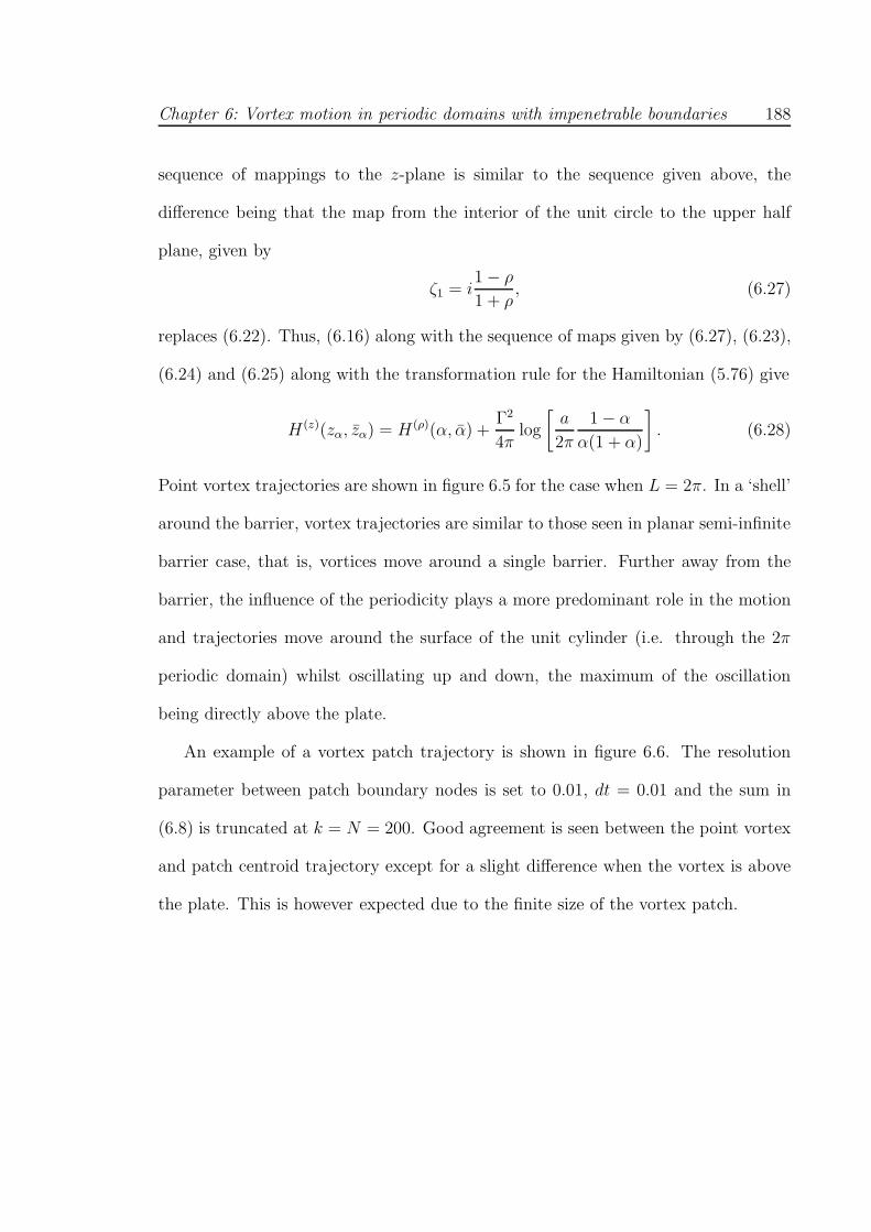
Chapter 6: Vortex motion in periodic domains with impenetrable boundaries 188
sequence of mappings to the z-plane is similar to the sequence given above, the
difference being that the map from the interior of the unit circle to the upper half
plane, given by
ζ1 = i1 − ρ
1 + ρ, (6.27)
replaces (6.22). Thus, (6.16) along with the sequence of maps given by (6.27), (6.23),
(6.24) and (6.25) along with the transformation rule for the Hamiltonian (5.76) give
H(z)(zα, zα) = H(ρ)(α, α) +Γ2
4πlog
[
a
2π
1 − α
α(1 + α)
]
. (6.28)
Point vortex trajectories are shown in figure 6.5 for the case when L = 2π. In a ‘shell’
around the barrier, vortex trajectories are similar to those seen in planar semi-infinite
barrier case, that is, vortices move around a single barrier. Further away from the
barrier, the influence of the periodicity plays a more predominant role in the motion
and trajectories move around the surface of the unit cylinder (i.e. through the 2π
periodic domain) whilst oscillating up and down, the maximum of the oscillation
being directly above the plate.
An example of a vortex patch trajectory is shown in figure 6.6. The resolution
parameter between patch boundary nodes is set to 0.01, dt = 0.01 and the sum in
(6.8) is truncated at k = N = 200. Good agreement is seen between the point vortex
and patch centroid trajectory except for a slight difference when the vortex is above
the plate. This is however expected due to the finite size of the vortex patch.
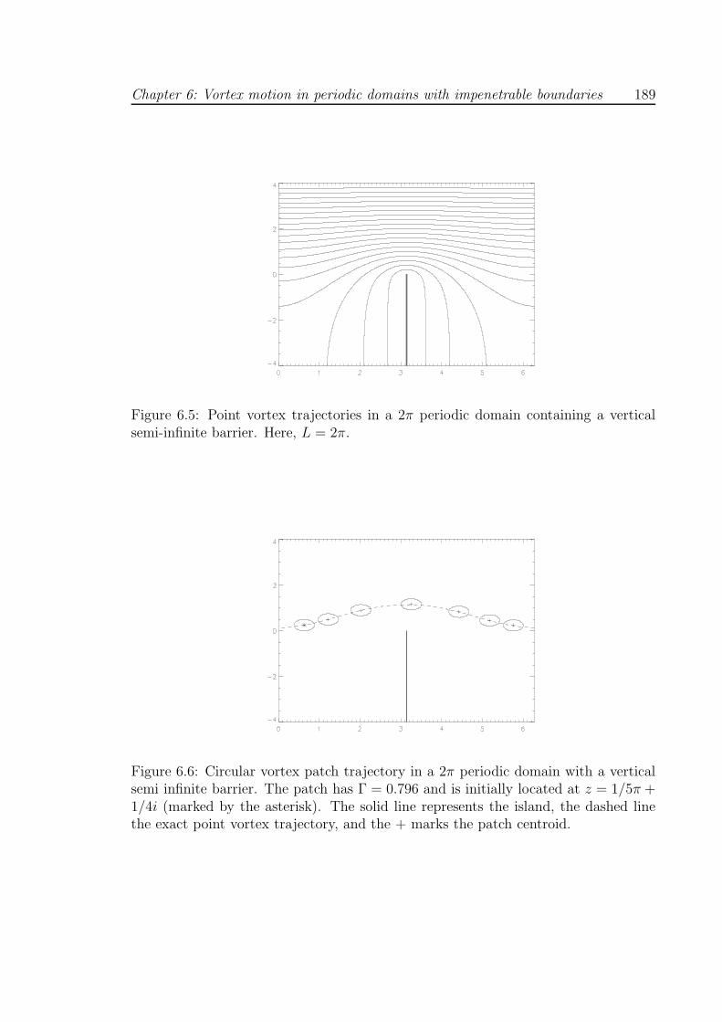
Chapter 6: Vortex motion in periodic domains with impenetrable boundaries 189
Figure 6.5: Point vortex trajectories in a 2π periodic domain containing a verticalsemi-infinite barrier. Here, L = 2π.
Figure 6.6: Circular vortex patch trajectory in a 2π periodic domain with a verticalsemi infinite barrier. The patch has Γ = 0.796 and is initially located at z = 1/5π +1/4i (marked by the asterisk). The solid line represents the island, the dashed linethe exact point vortex trajectory, and the + marks the patch centroid.
Chapter 6: Vortex motion in periodic domains with impenetrable boundaries 190
6.4 Summary
In this chapter, a method for computing the motion of vortices in periodic strips
(or on the surface of the unit cylinder) with boundaries has been presented. The
methods for computing these motions are similar to those presented in chapter 5.
Here, two singly connected domains were considered, an array horizontal thin is-
lands and an array of semi-infinite vertical barriers. Vortex trajectories close to the
boundaries were, in both cases, similar to the planar cases involving a single vortex
and an isolated boundary. Further away from the boundaries the periodicity of the
configuration plays a predominant role in the dynamics.
Good agreement is seen between contour dynamics and point vortex trajectories
in cases when the patch remains close to circular. Again, the principle of the method
presented here can be extended to doubly connected periodic domains, using the
methods of chapter 5.3, and potentially domains of a higher connectivity. Although,
in such cases, the required mappings may not be as straightforward as for non-periodic
cases in domains of a higher connectivity.
Chapter 7
Conclusions and future work
Analytical and numerical methods have been applied to a number of problems
involving two dimensional, inviscid and incompressible flows with regions of constant
vorticity. Broadly speaking, the work has considered three types of problem. In
chapters 2 and 3 the shapes of equilibria for point vortices near a vorticity interface
were found analytically in the linear limit of small amplitude interfacial waves and
numerically for fully non-linear systems respectively. Chapter 4 considered the time-
dependent problem of a vortex-wave interaction on the surface of the sphere and
chapters 5 and 6 considered the motion of vortices in bounded domains on the surface
of the sphere and in a 2π-singly-periodic strip respectively.
For the systems considered in chapter 2 the vorticity was generated by a shear flow.
The first system considered was the planar problem of two point vortices of opposite
signed circulations either side of the vorticity interface, that is, the anti-symmetric
analogue of that considered in McDonald (2004). In contrast to McDonald (2004) it
was shown in the linear limit it is not possible to construct such an equilibrium. A
191
Chapter 7: Conclusions and future work 192
non-linear analogue of this equilibrium could also not be found.
A series of periodic configurations were then considered. The configurations in-
cluded a periodic array of vortices located near an interface in the irrotational region
of the flow, a periodic array of vortices located near an interface in the rotational re-
gion of the flow and an array of anti-symmetrically placed vortices of opposite signed
circulation either side of the interface. A range of equilibria shapes were found for
these configurations. When vortices were placed in the irrotational region of the flow
there tended to be a peak in the interface placed directly above the point vortex.
In contrast, when the vortices were placed in the rotational region of the flow the
maximum height of the interface was in between the vortices and the minimum lo-
cated above the vortices. For the anti-symmetric periodically placed vortex case,
equilibrium shapes were found to be dominated by the primary mode, that is, they
resembled a full sine wave per period. However, surprisingly, the interface tended to
‘sink’ towards vortices with a positive circulation and be ‘pushed away’ from vortices
with a negative circulation. This behaviour is contrast to what is generally observed
in many non-periodic systems.
In chapter 3 a combination of contour dynamics and Newtonian iteration was
used to compute the corresponding non-linear equilibria to those found in chapter 2.
Computational equilibria shapes generally agreed very well with those found in the
linear limit. The computed equilibria were also shown to be robust by using them
as initial conditions in a time dependent contour dynamics code. Small amplitude
equilibria would remain largely unchanged over very long periods of time while larger
amplitude equilibria in which much higher velocity fields were present would remain
Chapter 7: Conclusions and future work 193
relatively stationary for reasonable periods of time before slowly deforming.
In chapter 4 the time evolution of a system consisting of single point vortex on
the surface of the unit sphere interacting with an initially flat vorticity interface was
examined. A system of first order ODEs was derived in the linear limit of small
amplitude waves at the interface. This system of ODEs was integrated numerically
to examine the behaviour of the system. Further approximations yield analytical
solutions governing the initial movements of the system. Such approximations also
give insight into the stability of vortices located at the two poles. The main results
predicted by linear theory indicate that a point vortex in a sea of same signed vorticity
will initially move away from the vorticity interface whilst a vortex in a sea of opposite
signed vorticity will move towards it. This result leads to the conclusion that a vortex
placed at a pole in a sea of same signed vorticity is at a stable equilibrium and vice
versa. This result is confirmed by an analytical, non-linear, stability analysis.
Evolution of the fully non-linear system is again explored using contour dynamics.
In highly linear cases or over short time periods contour dynamics is in very good
agreement with linear theory. Computations also show that ‘intermediate’ strength
vortices exhibit a drift away from the interface when surrounded by a sea of same
signed vorticity and towards the interface when surrounded by a sea of opposite signed
vorticity. Intermediate is used here in the sense that the system cannot be described
by linear theory over long periods of time but where the vortex is sufficiently strong
to induce rapid contour wrapping. As discussed in Polvani and Dritschel (1993) this
model is, to first order, relevant to studying the dynamics in Saturn’s atmosphere
and may provide a dynamical explanation behind the location of Saturn’s polar storm
Chapter 7: Conclusions and future work 194
discovered in recent observations (Dyudina et al. 2009).
The final two chapters investigate the motion of vortices in domains with impen-
etrable boundaries. Vortex motion on the surface of the unit sphere is considered in
chapter 5 and motion on the unit cylinder or, equivalently, 2π-singly-periodic domain
in chapter 6. The methodology employed in each chapter is similar. Contour dynam-
ics algorithms formulated in their respective topographies are used to calculate the
flow in the required domain as if boundaries are not present. Utilizing the invari-
ance of Laplace’s equation under conformal mapping, the boundary value problem is
mapped to the exterior of the unit circle and an irrotational flow field found, such
that, when added to that owing to the vortices in the absence of boundaries satisfies
the boundary conditions in the original domain. The main difference in computing
motion in the respective domains (apart from the different contour dynamics algo-
rithm) is that the spherical problem is projected into the stereographic plane and
requires careful consideration of the quantities conserved under projection while the
periodic problem makes use of a log map to map the plane into the periodic domain.
On the sphere, vortex motion in a number of singly connected domains is pre-
sented. Further doubly connected examples of a barrier with two gaps are also pre-
sented. In cases where the vortex remained close to circular, the centroid of the patch
followed the corresponding point vortex trajectories very closely. This is as expected
as the velocity field exterior to a circular vortex patch is identical to that of a point
vortex of same circulation. In cases where background flows were included and in
the doubly connected case, some examples of vortex splitting were observed. In the
periodic problems considered on the surface of the unit cylinder, patch centroid and
Chapter 7: Conclusions and future work 195
point vortex trajectories are again in very good agreement. An alternative procedure
for computing the motion of vortices in domains of potentially arbitrary connectivity
on a spherical shell is presented in Surana and Crowdy (2008).
An obvious problem to now consider is that of adapting the algorithm presented
in chapters 5 and 6 to work in domains of higher connectivity. To do this, a method
such as that discussed in Bird and Steele (1992) could be employed. Preliminary work
to this end has already begun. It would also be desirable to have a ‘contour surgery’
algorithm working on the sphere and cylinder, thus allowing long time integration of
systems in which vortex splitting phenomenon occur. Such an algorithm has already
been completed but requires some ‘fine tuning’ to have it working correctly in all
cases.
Other problems of interest include the vortex flushing problem and the motion
of vortices in the presence of moving boundaries. An example of a vortex flushing
problem is that, if a vortex in the open ocean passes by close to a bay, without actually
entering the bay, what is the rate of mixing between the fluid in the bay with that
of the open ocean? The central idea and challenge here is to compute the motion of
irrotational (i.e. passive) fluid and to quantify the mixing between different regions.
Literature on the aforementioned topics is currently sparse but both problems are
of interest to oceanographers. Additionally, for certain problems such as the vortex
flushing problem, an interesting exercise would be to compare results given by vortex
dynamics to those obtained from a general circulation model such as ICOM. More
‘direct’ comparisons between fundamental and general circulation models could help
clarify the interplay between various parameters in a general circulation models.
Appendix A
Implementation of spherical and
cylindrical contour dynamics
algorithms
Details on the implementation of a 2D contour dynamics algorithm are given in
Dritschel (1989). Below, details on implementing contour dynamics algorithms on the
surface of the unit sphere and on the surface of the unit cylinder with no boundaries
present are outlined. The following is based on Dritschel (1989), while the actual
construction of the associated numerical routines was done by the author.
A.1 Spherical contour dynamics
In general, to follow the motion of a distribution of vorticity is it necessary to
invert the Green’s function in the domain in question and use the resulting velocity
196
Appendix A: Implementation of spherical and cylindrical contour dynamicsalgorithms 197
field to advect the the fluid. The Green’s function for the motion of an inviscid,
incompressible fluid on the surface of the unit sphere is given by
G(θ, φ; θ′, φ′) =1
4πlog(1 − cos Θ), (A.1)
where θ is the co-latitude, φ the longitude and cos Θ = (cos θ cos θ′+sin θ sin θ′ cos(φ−
φ′) is the inner product of the Cartesian coordinate vectors x = (sin θ cosφ, sin θ sinφ, cos θ)
and x′ = (sin θ′ cosφ′, sin θ′ sinφ′, cos θ′). On the surface of the sphere, the Gauss con-
straint requires that the vorticity ω satisfies
∫ 2π
0
∫ π
0
ωdθdφ = 0. (A.2)
The constraint (A.2) is built into (A.1) and the streamfunction is therefore given by
ψ(θ, φ) =1
4π
∫ ∫
ω(θ′, φ′) log(1 − cos Θ)dΩ′, (A.3)
where dΩ′ = sin θ′dθ′dφ′ is the incremental solid angle area.
The equations of contour dynamics will now be formulated for a single piecewise
constant patch of vorticity whose boundary is denoted C. Identical equations can
then be applied to any additional distributions of vorticity within the domain. Whilst
traversing the contour C in the anti-clockwise direction, label the change in vorticity
between the left hand and right hand sides of the contour by ω.
The azimuthal and longitudinal velocities in spherical polar coordinate can be
written as
dθ
dt= uθ = − 1
sin θ
∂ψ
∂φ, (A.4a)
sin θdφ
dθ= uφ =
∂ψ
∂θ. (A.4b)
Appendix A: Implementation of spherical and cylindrical contour dynamicsalgorithms 198
Substitution of (A.3) in (A.4a) and using Green’s theorem gives
uθ = − ω
4π
∫
C
log(1 − cos Θ) sin θ′dθ′. (A.5)
Now, instead of deriving a similar equation for uφ, consider the following. In terms
of Cartesian coordinates, |x| = 1 and |x′| = 1 giving 1 − cos Θ = 12|x − x′|2. Then,
noting that − sin θdθ = dz, (A.5) can be written as
dz
dt= − ω
2π=
∫
C
log |x − x′|dz′. (A.6)
Thus, by symmetry, the three Cartesian velocities must be given by
dx
dt= − ω
2π=
∫
C
log |x − x′|dx′. (A.7)
The contour C is represented as a number of discrete nodes where interpolation be-
tween nodes takes the form of a cubic spline. The shape of the contour between
adjacent nodes, say i and i+ 1, can be written as
x(p) = xi + pti + η(p)ni + ζ(p)si, (A.8a)
ti = xi+1 − xi, (A.8b)
ni = xi × xi+1, (A.8c)
si = (xi + xi+1)/2, (A.8d)
η(p) = αip + βip2 + γip
3, (A.8e)
Appendix A: Implementation of spherical and cylindrical contour dynamicsalgorithms 199
ζ(p) =1
2e2i p(1 − p), (A.8f)
where 0 ≤ p ≤ 1 is the fractional distance between the nodes and ei = |ti| =
(dx2i + dy2
i + dz2i )
12 . The coefficients αi, βi and γi are calculated according to
αi = −1
3eiki −
1
6eiki+1, (A.9a)
βi = −1
2eiki, (A.9b)
γi =1
6ei(ki+1 − ki), (A.9c)
where ki is the curvature at the ith node and is given explicitly by
ki =2xi · (ti × ti−1)
|tie2i−1 + ti−1e2i |. (A.10)
Additionally, using (A.10) the local density of nodes then takes the form
ρi = (µ)−1(1 + ki)a2 , (A.11)
where µ is a small non-dimensional number and a is the resolution parameter between
nodes. The resolution parameter a controls how sharply the local node density ρi
increases with curvature ki.
Substituting (A.8a) into (A.7) the velocity field u = dx/dt at a point x can be
represented as the the sum of contributions to the velocity field from contour segments
(∆ui) adjoining all adjacent nodes, that is
u =1
2π
∑
i
ω∆ui, (A.12)
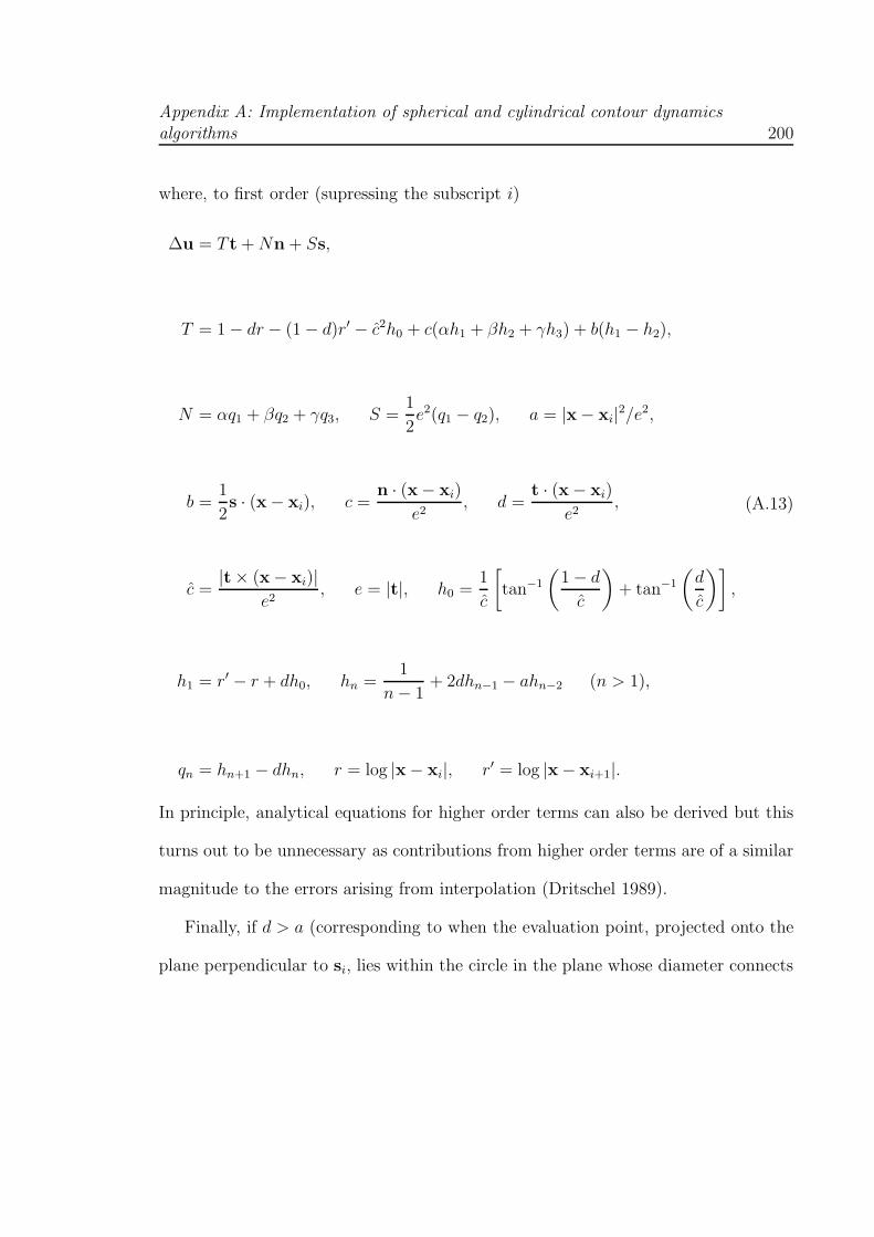
Appendix A: Implementation of spherical and cylindrical contour dynamicsalgorithms 200
where, to first order (supressing the subscript i)
∆u = T t +Nn + Ss,
T = 1 − dr − (1 − d)r′ − c2h0 + c(αh1 + βh2 + γh3) + b(h1 − h2),
N = αq1 + βq2 + γq3, S =1
2e2(q1 − q2), a = |x − xi|2/e2,
b =1
2s · (x − xi), c =
n · (x − xi)
e2, d =
t · (x − xi)
e2,
c =|t× (x − xi)|
e2, e = |t|, h0 =
1
c
[
tan−1
(
1 − d
c
)
+ tan−1
(
d
c
)]
,
h1 = r′ − r + dh0, hn =1
n− 1+ 2dhn−1 − ahn−2 (n > 1),
qn = hn+1 − dhn, r = log |x − xi|, r′ = log |x − xi+1|.
(A.13)
In principle, analytical equations for higher order terms can also be derived but this
turns out to be unnecessary as contributions from higher order terms are of a similar
magnitude to the errors arising from interpolation (Dritschel 1989).
Finally, if d > a (corresponding to when the evaluation point, projected onto the
plane perpendicular to si, lies within the circle in the plane whose diameter connects
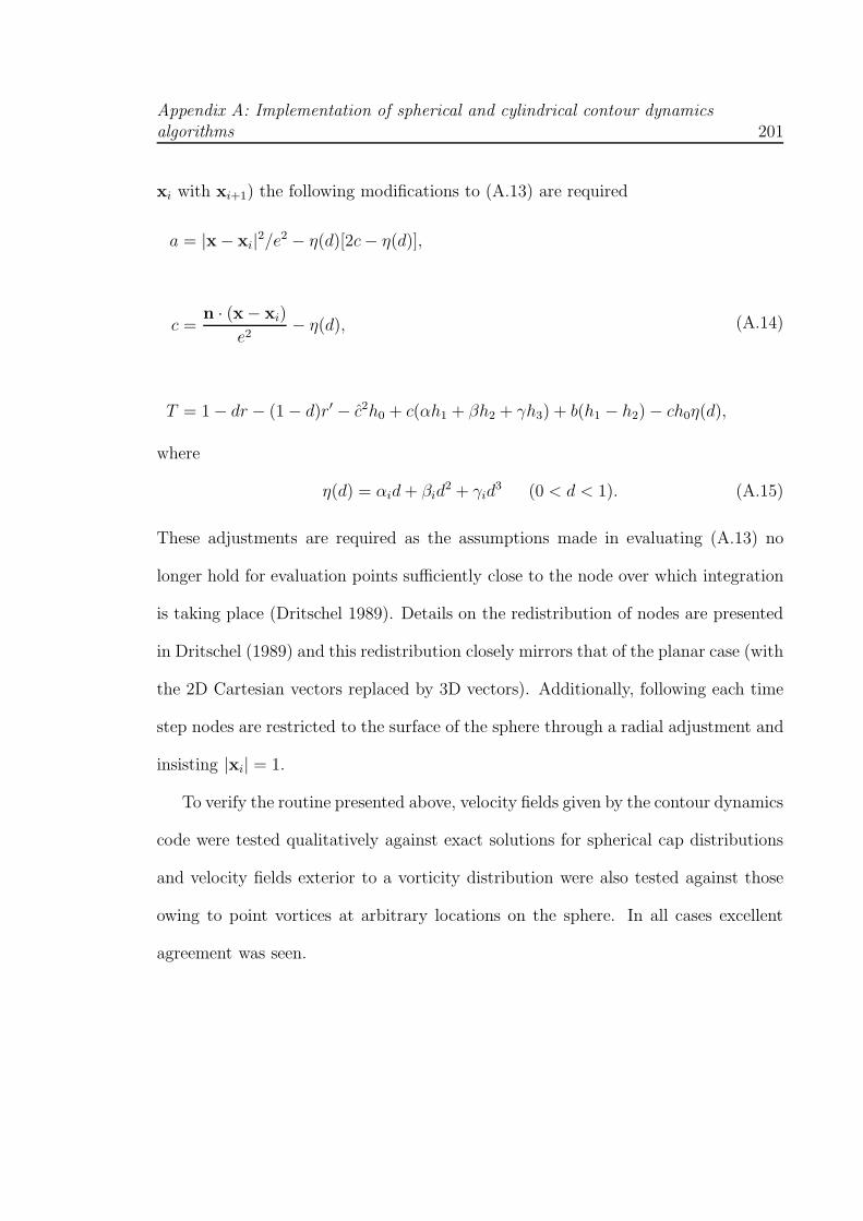
Appendix A: Implementation of spherical and cylindrical contour dynamicsalgorithms 201
xi with xi+1) the following modifications to (A.13) are required
a = |x − xi|2/e2 − η(d)[2c− η(d)],
c =n · (x − xi)
e2− η(d),
T = 1 − dr − (1 − d)r′ − c2h0 + c(αh1 + βh2 + γh3) + b(h1 − h2) − ch0η(d),
(A.14)
where
η(d) = αid+ βid2 + γid
3 (0 < d < 1). (A.15)
These adjustments are required as the assumptions made in evaluating (A.13) no
longer hold for evaluation points sufficiently close to the node over which integration
is taking place (Dritschel 1989). Details on the redistribution of nodes are presented
in Dritschel (1989) and this redistribution closely mirrors that of the planar case (with
the 2D Cartesian vectors replaced by 3D vectors). Additionally, following each time
step nodes are restricted to the surface of the sphere through a radial adjustment and
insisting |xi| = 1.
To verify the routine presented above, velocity fields given by the contour dynamics
code were tested qualitatively against exact solutions for spherical cap distributions
and velocity fields exterior to a vorticity distribution were also tested against those
owing to point vortices at arbitrary locations on the sphere. In all cases excellent
agreement was seen.
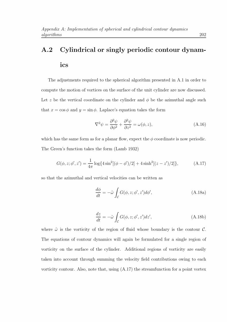
Appendix A: Implementation of spherical and cylindrical contour dynamicsalgorithms 202
A.2 Cylindrical or singly periodic contour dynam-
ics
The adjustments required to the spherical algorithm presented in A.1 in order to
compute the motion of vortices on the surface of the unit cylinder are now discussed.
Let z be the vertical coordinate on the cylinder and φ be the azimuthal angle such
that x = cosφ and y = sinφ. Laplace’s equation takes the form
∇2ψ =∂2ψ
∂φ2+∂2ψ
∂z2= ω(φ, z), (A.16)
which has the same form as for a planar flow, expect the φ coordinate is now periodic.
The Green’s function takes the form (Lamb 1932)
G(φ, z;φ′, z′) =1
4πlog4 sin2[(φ− φ′)/2] + 4 sinh2[(z − z′)/2], (A.17)
so that the azimuthal and vertical velocities can be written as
dφ
dt= −ω
∫
C
G(φ, z;φ′, z′)dφ′, (A.18a)
dz
dt= −ω
∫
C
G(φ, z;φ′, z′)dz′, (A.18b)
where ω is the vorticity of the region of fluid whose boundary is the contour C.
The equations of contour dynamics will again be formulated for a single region of
vorticity on the surface of the cylinder. Additional regions of vorticity are easily
taken into account through summing the velocity field contributions owing to each
vorticity contour. Also, note that, using (A.17) the streamfunction for a point vortex
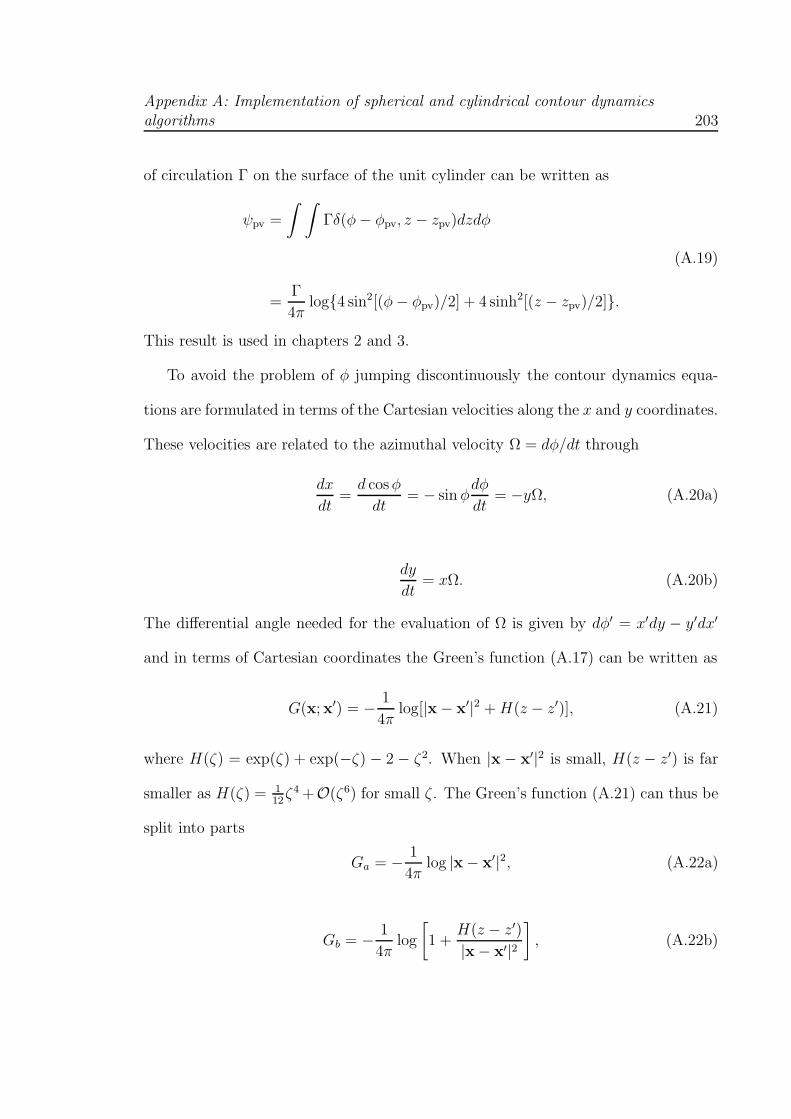
Appendix A: Implementation of spherical and cylindrical contour dynamicsalgorithms 203
of circulation Γ on the surface of the unit cylinder can be written as
ψpv =
∫ ∫
Γδ(φ− φpv, z − zpv)dzdφ
=Γ
4πlog4 sin2[(φ− φpv)/2] + 4 sinh2[(z − zpv)/2].
(A.19)
This result is used in chapters 2 and 3.
To avoid the problem of φ jumping discontinuously the contour dynamics equa-
tions are formulated in terms of the Cartesian velocities along the x and y coordinates.
These velocities are related to the azimuthal velocity Ω = dφ/dt through
dx
dt=d cosφ
dt= − sin φ
dφ
dt= −yΩ, (A.20a)
dy
dt= xΩ. (A.20b)
The differential angle needed for the evaluation of Ω is given by dφ′ = x′dy − y′dx′
and in terms of Cartesian coordinates the Green’s function (A.17) can be written as
G(x;x′) = − 1
4πlog[|x − x′|2 +H(z − z′)], (A.21)
where H(ζ) = exp(ζ) + exp(−ζ) − 2 − ζ2. When |x − x′|2 is small, H(z − z′) is far
smaller as H(ζ) = 112ζ4 +O(ζ6) for small ζ . The Green’s function (A.21) can thus be
split into parts
Ga = − 1
4πlog |x − x′|2, (A.22a)
Gb = − 1
4πlog
[
1 +H(z − z′)
|x − x′|2]
, (A.22b)
Appendix A: Implementation of spherical and cylindrical contour dynamicsalgorithms 204
to ensure the Green’s function is well behaved for small |x− x′|2. Integrals involving
Ga can then be integrated explicitly to obtain equations similar to those for the
sphere (A.13). Denote the velocity owing to this singular part of the Green’s function
ua. Integrals involving Gb are evaluated using numerical quadrature and denote the
velocity field owing to this non-singular part of the Green’s function ub.
As mentioned above, the explicit velocity field owing to integrals involving Ga
yields very similar results to (A.13). The required modifications to the spherical
algorithm are detailed below. For the shape of the contour between adjacent nodes,
some minor modifications are required. In (A.8) si = (12(xi + xi+1),
12(yi + yi+1), 0)
replaces (A.8d) (i.e. the z-component is set to zero owing to the lack of curvature in
the z-direction), ni = si × ti replaces (A.8c) and e2i = dx2i + dy2
i is used in place of e2i
in (A.8f) only. Similarly, xi = (xi, yi, 0) replaces xi = (xi, yi, zi) in (A.10).
Substituting the modified version of (A.8) into (A.18) and noting that dz′/dp =
dzi + (dη/dp)nzi and dφ′/dp = nzi − (dη/dp)dzi + [ζ − (p− 12)dζ/dp]nzi (to first order
in η and ζ), the singular part of the Green’s function Ga yields
Ωa =1
2π
∑
i
ωi[(Ti + Si)nzi −Nidzi], (A.23a)
wa =1
2π
∑
i
ωi[Tidzi +Ninzi], (A.23b)
where u = −yΩ and v = xΩ. Ti and Ni in (A.23) have the same form as in (A.13)
and Si is modified to
Si =1
4e2(q1 − q2 +
2
3q3). (A.24)
It now remains to determine ub, the velocity field owing to the non-singular part of
the Green’s function, Gb. Ωb and wb can be evaluated using three-point Gaussian
Appendix A: Implementation of spherical and cylindrical contour dynamicsalgorithms 205
quadrature,
Ωb =1
2π
∑
i
ωi
3∑
l=1
σlGb(x;x′(pl))dφ′
dp(pl), (A.25a)
wa =1
2π
∑
i
ωi
3∑
l=1
σlGb(x;x′(pl))dz′
dp(pl), (A.25b)
where p1 = 0.112701665379..., p2 = 0.5 and p3 = 1 − p1, σ1 = 5/18, σ2 = 8/18 and
σ3 = σ1 (Abramowitz and Stegun 1965). The total velocity field is then given by
u = ua + ub. (A.26)
Similar to in the spherical case, nodes tend to displace slightly from the cylinder due
to numerical errors and thus following time step the x and y coordinates at each node
are rescaled such that x2i + y2
i = 1. Again, to verify the algorithm, quantitative tests
in which velocity fields exterior to small patches were tested against those owing to
point vortices were carried out. Excellent agreement was seen.
Appendix B
The generation of potential
vorticity gradients by step
topography
For simplicity, consider the motion of a 2D, homogeneous, inviscid fluid governed
by the shallow water equations
Du
Dt= −∇p, (B.1a)
∂H
∂t+ ∇ · (Hu) = 0, (B.1b)
where u = (u, v) are the horizontal velocity components, the material derivate is given
by D/Dt = ∂t +u ·∇ and p is the pressure owing to the change in depth H = h−hB
where h is the fluid surface height and hB is the height at the fluid base. Note that
(B.1a) and (B.1b) represent the shallow water equations in a non-rotating frame and
thus the effect of the Earth’s rotation has been neglected. A more complete treatment
206
Appendix B: The generation of potential vorticity gradients by step topography 207
of the shallow water equations (with rotation included) is given in Pedlosky (1987).
The vertical component of vorticity is given by
ω = (∇× u) · k = ux − uy. (B.2)
Taking the curl of (B.1a) gives
ωt + u · ∇ω + ω∇ · u = 0, (B.3)
and, from using (B.1b)
Dq
Dt= 0, (B.4)
where q = ω/H is the potential vorticity. The potential vorticity q associated with
each fluid parcel is thus a constant of the motion, i.e. if a fluid particle moves from
deep to shallow water, its vorticity must decrease.
Bibliography
Abramowitz, M. and I. A. Stegun, 1965: Handbook of Mathematical Functions .
Dover, New York.
Acheson, D. J., 1990: Elementary Fluid Dynamics . Oxford University Press.
Aref, H., 2007: Vortices and polynomials. Fluid Dynamics Research, 39, 5–23.
Aref, H., P. K. Newton, M. A, Stremler, T. Tokieda, and D. L. Vainchtein, 2003:
Vortex Crystals. Advances in Appl. Mech., 39, 1–79.
Armi, L., D. Hebert, N. Oakey, J. F. Price, P. L. Richardson, H. T. Rossby, and
B. Ruddick, 1989: Two years in the life of a Mediterranean salt lens. J. Phys.
Oceanogr., 19, 354.
Atassi, O. V., 1998: Analytical and numerical study of the nonlinear interaction
between a point vortex and a wall-bounded shear layer. J. Fluid Mech., 373, 155–
192.
B A Smith, t., 1982: A new look at the Saturn system: the Voyager 2 images.
Science, 215, 504–537.
208
Bibliography 209
Bell, G. I., 1990: Interaction between vortices and waves in a simple model of
geophysical flow. Phys. Fluids A, 2, 575–585.
Bird, M. D. and C. R. Steele, 1992: A Solution Procedure for Laplace’s Equation
on Multiply Connected Circular Domains. J. Appl. Mech., 59, 398.
Crowdy, D., 1999: A class of exact multipolar vortices. Phys. Fluids , 11, 2556–2564.
— 2002a: Exact solutions for rotating vortex arrays with finite-area cores. J. Fluid
Mech., 469, 209–235.
— 2002b: The construction of exact multipolar equilibria of the two-dimensional
Euler equations. Phys. Fluids , 14, 257–267.
— 2006: Point vortex motion on the surface of a sphere with impenetrable bound-
aries. Phys. Fluids , 18, 036602.
Crowdy, D. and M. Cloke, 2003: Analytical solutions for distributed multipolar
vortex equilibria on a sphere. Phys. Fluids , 15, 22–34.
Crowdy, D. and J. Marshall, 2004: Growing vortex patches. Phys. Fluids , 16, 3122.
Crowdy, D. and A. Surana, 2008: Contour dynamics in complex domains. J. Fluid
Mech., 593, 235–254.
Crowdy, D. G. and J. S. Marshall, 2005: The motion of a point vortex around
multiple circular islands. Phys. Fluids , 17.
— 2006: The motion of a point vortex through gaps in walls. J. Fluid Mech., 551,
31–48.
Bibliography 210
Deem, G. S. and N. J. Zabusky, 1978: ‘V-states’, interactions, recurrence and break-
ing. Phys. Rev. Lett., 40, 859–862.
DeFelice, T. P., J. D. Meyer, G. Xian, J. Christopherson, and R. F. Cahalan, 2000:
Landsat 7 reveals more than just surface features in remote areas of the globe. Bull.
Amer. Meteor. Soc., 81, 1047–1049.
Domm, U., 1956: Uber die Wirbelstaßen von geringster Instabilitat. Zeitschrift fur
Angewandte Mathematik und Mechanik , 36, 367–371.
Dritschel, D. G., 1988: Contour dynamics/surgery on the sphere. J. Comput. Phys.,
79, 477–483.
— 1989: Contour dynamics and contour surgery: Numerical algorithms for ex-
tended, high-Resolution modelling of vortex dynamics in two-dimensional, inviscid,
incompressible flows. Computer Physics Reports , 10, 77–146.
Dritschel, D. G. and L. M. Polvani, 1992: The roll-up of vorticity strips on the
surface of a sphere. J. Fluid Mech., 234, 47–69.
Dunn, D. C., N. R. McDonald, and E. R. Johnson, 2001: The motion of a singular
vortex near an escarpment. J. Fluid Mech., 448, 335–365.
Dyudina, U. A., A. P. Ingersoll, S. P. Ewald, A. R. Vasavada, R. A. West, K. H.
Baines, T. W. Momary, A. D. D. Geino, J. M. Barbara, C. C. Porco, R. K. Achter-
berg, F. M. Flasar, A. A. Simon-Miller, and L. N. Fletcher, 2009: Saturn’s south
polar vortex compared to other large vortices in the Solar System. Icarus, 202,
240–248.
Bibliography 211
Fratantoni, D., W. Johns, and T. Townsend, 1995: Rings of the North Brazil Cur-
rent. J. Geophys. Res., 100, 10633–10654.
Gascard, J. C., A. J. Watson, M. Messias, K. A. Olsson, T. Johannessen, and K. Si-
monsen, 2002: Long-lived vortices as a mode of deep ventilation in the Greenland
Sea. Nature, 416, 525–527.
Gradshteyn, I. S. and I. M. Ryzhik, 1965: Table of integrals series and products.
Academic Press, New York and London.
Hughes, T. J. R., 2003: The Finite Element Method . Dover Publications Inc.
Johnson, E. R. and N. R. McDonald, 2004a: The motion of a vortex near a gap in
a wall. Phys. Fluids , 16, 462–469.
— 2004b: The motion of a vortex near two circular cylinders. Proc. R. Soc. Lond.
A, 460, 939–954.
— 2005: Vortices near barriers with multiple gaps. J. Fluid Mech., 531, 335–358.
Juckes, M. N. and M. E. McIntyre, 1987: A high-resolution one-layer model of
breaking planetary waves in the stratosphere. Nature, 328, 590.
Kelvin, L., 1878: Floating magnets (illustrating vortex systems). Collected works,
IV, 135–40.
Kidambi, R. and P. K. Newton, 2000: Point vortex motion on a sphere with solid
boundaries. Phys. Fluids , 12, 581–588.
Lamb, H., 1932: Hydrodynamics. Cambridge Univ. Press..
Bibliography 212
McDonald, N. R., 1998: The motion of an intense vortex near topography. J. Fluid
Mech., 367, 359–377.
— 2002: Steady, nonradiating geophysical flow past a cylinder with circulation.
Phys. Fluids , 14, 3018–3027.
— 2004: A new translating quasigeostrophic V-state. European Journal of Mechanics
B/Fluids , 23, 633–644.
— 2008: Vortex equilibria in flow past a plate. ANZIAM J., 49, 347–359.
McWilliams, J. C., 1985: Submeoscale, coherent vortices in the ocean. Rev. Geo-
phys., 23, 165–182.
Meleshko, V. V. and G. J. F. V. Heijst, 1994: On Chaplygin’s investigations of two-
dimensional vortex structures in an inviscid fluid. J. Fluid Mech., 272, 157–182.
Nelson, R. B. and N. R. McDonald, 2009a: Finite area vortex motion on a sphere
with impenetrable boundaries. Phys. Fluids , 21, 016602.
— 2009b: Vortex motion on a sphere: barrier with two gaps. Theor Comp Fluid
Dyn.
Newton, P. K. and T. Sakajo, 2007: The N -vortex problem on a rotating sphere. III.
Ring configurations coupled to a background flow. Proc. R. Soc. A, 463, 961–977.
Nof, D., 1995: Choked flows from the Pacific to the Indian Ocean. J. Phys.
Oceanogr., 25, 1369–1383.
Pedlosky, J., 1987: Geophysical Fluid Dynamics . Springer.
Bibliography 213
— 1994: Stratified abyssal flow in the presence of fractured ridges. J. Phys.
Oceanogr., 30, 403–417.
Pierrehumbert, R. T., 1980: A family of steady, translating vortex pairs with dis-
tributed vorticity. J. Fluid Mech., 99, 129–144.
Polvani, L. M. and D. G. Dritschel, 1993: Wave and vortex dynamics on the surface
of a sphere. J. Fluid Mech., 225, 35–64.
Saffman, P. G., 1992: Vortex Dynamics. Cambridge University Press, Cambridge.
Scullen, D. and E. O. Tuck, 1995: Nonlinear free-surface flow computations for
submerged cylinders. J. Ship Res., 39, 185.
Sheremet, V. A., 2001: Hysteresis of a western boundary current leaping across a
gap. J. Phys. Oceanogr., 31, 1247–1259.
Smith, G. D., 1985: Numerical Solution of Partial Differential Equations: Finite
Difference Methods. Clarendon Press.
Stern, M. E. and G. R. Flierl, 1987: On the interaction of a vortex with a shear
flow. J. Geophys. Res., 92, 10,733–10,744.
Surana, A. and D. Crowdy, 2008: Vortex dynamics in complex domains on a spher-
ical surface. Journal of Computational Physics , 227, 6058–6070.
Thomson, J. J., 1883: A treatise on the motion of vortex rings. Macmillan.
Versteeg, H. and W. Malalasekra, 1995: An Introduction to Computational Fluid
Dynamics: The Finite Volume Method . Prentice Hall.
Bibliography 214
von Karman, T. and H. L. Rubach, 1913: Uber den Mechanismus des Flussigkeitsund
Luftwidertands. Phys. Z , 13, 49–59.
Webster, R., 2006: Stability of Navier-Stokes discretizations on collocated meshes of
high anisotropy and the performance of algebraic multigrid solvers. Int. J. Numer.
Meth. Fluids , 51, 14191438.
White, A. J. and N. R. McDonald, 2004: The Motion of a Point Vortex near Large-
Amplitude Topography in a Two-Layer Fluid. J. Phys. Oceanogr., 34, 2808–2824.
Wu, H. M., E. A. Overman, and E. A. Zabusky, 1984: Steady state solutions of the
Euler equations in two dimensions. Rotating and translating V-states with limiting
cases. J. Comput. Phys., 53, 42–71.