DI

SC

US

SI

ON

P

AP

ER

S

ER

IE

S

Forschungsinstitut zur Zukunft der ArbeitInstitute for the Study of Labor

Moderating Political Extremism:Single Round vs Runoff Elections under Plurality Rule

IZA DP No. 7561

August 2013

Massimo BordignonTommaso NanniciniGuido Tabellini

Moderating Political Extremism: Single Round vs Runoff Elections

under Plurality Rule

Massimo Bordignon Università Cattolica del Sacro Cuore

and CESifo

Tommaso Nannicini IGIER, Bocconi University

and IZA

Guido Tabellini IGIER, Bocconi University, CIFAR, CEPR and CESifo

Discussion Paper No. 7561 August 2013

IZA

P.O. Box 7240 53072 Bonn

Germany

Phone: +49-228-3894-0 Fax: +49-228-3894-180

E-mail: iza@iza.org

Any opinions expressed here are those of the author(s) and not those of IZA. Research published in this series may include views on policy, but the institute itself takes no institutional policy positions. The IZA research network is committed to the IZA Guiding Principles of Research Integrity. The Institute for the Study of Labor (IZA) in Bonn is a local and virtual international research center and a place of communication between science, politics and business. IZA is an independent nonprofit organization supported by Deutsche Post Foundation. The center is associated with the University of Bonn and offers a stimulating research environment through its international network, workshops and conferences, data service, project support, research visits and doctoral program. IZA engages in (i) original and internationally competitive research in all fields of labor economics, (ii) development of policy concepts, and (iii) dissemination of research results and concepts to the interested public. IZA Discussion Papers often represent preliminary work and are circulated to encourage discussion. Citation of such a paper should account for its provisional character. A revised version may be available directly from the author.

IZA Discussion Paper No. 7561 August 2013

ABSTRACT

Moderating Political Extremism: Single Round vs Runoff Elections under Plurality Rule*

We compare single round vs runoff elections under plurality rule, allowing for partly endogenous party formation. Under runoff elections, the number of political candidates is larger, but the influence of extremist voters on equilibrium policy and hence policy volatility are smaller, because the bargaining power of the political extremes is reduced compared to single round elections. The predictions on the number of candidates and on policy volatility are confirmed by evidence from a regression discontinuity design in Italy, where cities above 15,000 inhabitants elect the mayor with a runoff system, while those below hold single round elections. JEL Classification: H72, D72, C14 Keywords: electoral rules, policy volatility, regression discontinuity design Corresponding author: Tommaso Nannicini Bocconi University Department of Economics Via Rontgen 1 20136 Milan Italy E-mail: tommaso.nannicini@unibocconi.it

* We thank Pierpaolo Battigalli, Daniel Diermeier, Massimo Morelli, Giovanna Iannantuoni, Francesco de Sinopoli, Ferdinando Colombo, Piero Tedeschi, Per Petterson-Lindbom, and seminar participants at CIFAR, the Universities of Brescia, Cattolica, Munich, Warwick, the Cesifo Workshop in Public Economics, the IGIER workshop in Political Economics, the IIPF annual conference, and the NYU conference in Florence for several helpful comments. We also thank Massimiliano Onorato for excellent research assistance, and Veruska Oppedisano, Paola Quadrio, and Andrea Di Miceli for assistance in collecting the data. Financial support is gratefully acknowledged from the Italian Ministry for Research and Catholic University of Milan for Massimo Bordignon, from ERC (grant No. 230088) and Bocconi University for Tommaso Nannicini, and from the Italian Ministry for Research, CIFAR, ERC (grant No. 230088), and Bocconi University for Guido Tabellini.

1 Introduction

In some electoral systems, citizens vote twice: in a first round they select a subset of

candidates, over which they cast a final vote in a second round. The system for electing

the French President, where the two candidates who get more votes in the first round are

admitted to the second round, is possibly the best known example. But variants of this

runoff (or dual ballot) system are increasingly used in many other countries, for example

in Latin America, in the US gubernatorial primary elections, and in many local elections,

including Italian municipal and provincial elections (see Cox, 1997, and Golder, 2005).

How does the runoff system differ from the more common single round (or single ballot)

plurality rule, where candidates are directly elected at the first round? In spite of its obvious

relevance, this question remains largely unaddressed, particularly when it comes to studying

the economic policies enacted under these two electoral systems.

This paper contrasts runoff vs single round elections under plurality rule, focusing on

the policy platforms that get implemented in equilibrium. We analyze a model where

parties with ideological preferences commit to a one-dimensional policy before the elections.

The number of parties is partly endogenous. We start out with four parties. Before the

elections, however, parties choose whether or not to merge, and bargain over the policy

platform that would result from merging. We obtain two main results. First, in equilibrium

the number of candidates is larger in the dual compared to the single ballot. Second, and

more importantly, the runoff system moderates the influence of extremist parties and voters

on the equilibrium policy, thereby inducing more centrist policies. The reason is that runoff

elections reduce the bargaining power of the extremist parties that typically appeal to a

smaller electorate. Intuitively, with a single round and under sincere voting, the extremes

can threaten to cause the electoral defeat of the nearby moderate candidate if this refuses

to strike an alliance. Under the runoff this threat is empty, provided that when the second

vote is cast some extremist voters are willing to vote for the closest moderate, rather than

abstain. This result holds even if renegotiation among parties is allowed between the two

rounds. Because of the larger influence of the political extremes, the equilibrium platforms

adopted by candidates with different political orientation are more distant between each

other under single round elections than under runoff. Therefore, conditional on the same

degree of political turnover, policy volatility is also expected to be higher in the former.

The model thus yields two general predictions: under runoff elections we should observe

more political candidates, but less policy volatility, compared to single round elections. We

take these predictions to the data, focusing on municipal elections in Italy. Since 1993,

Italian mayors are directly elected and have a prominent role in determining policy. Mu-

1

nicipalities below 15,000 inhabitants adopt a single round system, while a runoff system is

in place above this threshold. The data also reveal that voters are indeed mobile between

candidates: a relevant share of the voters supporting the excluded candidates seems to

participate again in the second round. This institutional setup thus allows us to test the

model’s predictions with a Regression Discontinuity Design (RDD).

We test the implications of our model with respect to both politics and policy. First,

we check whether the number of candidates for mayor is larger under the runoff system, as

opposed to the single round. The positive discontinuity at 15,000 is indeed large and statis-

tically significant: under runoff elections the number of candidates for mayor increases by

about 29%. Second, to test the prediction that runoff elections moderate political extrem-

ism and reduce policy volatility, we focus on one of the main policy tools of municipalities,

the business property tax. In 1993, with the introduction of this tax, Italian municipalities

were given large discretion in setting its tax rate, whose proceeds can be freely allocated to

all municipal functions, such as social assistance, housing, education, and so on.

The intuition for this test is simple. The size of government is influenced by ideology,

with left-wing governments generally raising more tax revenues and imposing higher business

property taxes (this is indeed confirmed by our data in the subsample of larger cities where

the political identity of the mayor is known). Hence, on average a change in the identity

of the mayor should lead to a sharper policy change where the influence of the extremist

parties is stronger, namely under single round elections. The RDD evidence supports this

prediction. We measure the volatility of the business property tax rate in two ways: by

the intertemporal variance (i.e., across legislative terms for the same municipality) and by

the cross-sectional variance (i.e., within population bins in the same year). Both indicators

display a negative discontinuity at 15,000, with less volatility above the threshold, which

is both large and statistically significant. The estimated coefficients point to an impact of

about 61% of runoff elections on the time series volatility of the tax rate, and an impact of

about 71% on the cross-sectional volatility around the population threshold.

Alternative explanations for this (reduced-form) effect on tax volatility are rejected by

our data, because the turnover between different mayors is similar in both runoff and single

round elections. Moreover, in a small and selected subsample of municipalities where we

can measure the political identity of parties, runoff elections have a negative impact on

the probability that the leftist political extreme—i.e., the Communist Party—joins the

main center-left coalition at the local level, in line with a direct implication of our model.

Overall, the empirical evidence thus supports the hypothesis that the runoff system reduces

the influence of the political extremes and induces policy moderation.

Our results have important implications for the design of democratic institutions. Po-

2

litical extremism is still widespread in many advanced and developing countries (including

Italy) and it is often counterproductive. It reduces ex-ante welfare if voters are risk averse,

and it induces sharp disagreement that often disrupts decision making in governments or

legislatures. In this respect, runoff electoral systems have an advantage over single round

elections, as they moderate the influence of extremist groups and reduce the welfare costs

associated with (partisan) policy volatility. While our findings mainly have a comparative

flavor, as they refer to multi-party environments, some of the implications might extend

to two-party systems, where—for instance—runoff primary elections have been proposed to

alleviate political extremism within the US parties (see Fiorina, 2005).

The existing literature on these issues is quite small. Some informal conjectures have

been advanced by institutionally oriented political scientists (Sartori, 1995; Fisichella, 1984).

Analytical work has mostly asked whether variants of Duverger’s Law or Hypothesis carry

over to the runoff system under strategic voting (Messner and Polborn, 2004; Cox, 1997;

Callander, 2005; Bouton, 2012; Bouton and Gratton, 2013 ).1 Less attention has instead

been devoted to the specific question of which policies are implemented in equilibrium. An

exception is Osborne and Slivinsky (1996). In a citizen-candidate model with sincere voting

and ideologically motivated candidates, they study equilibrium configuration of candidates

and policies in the two systems, concluding that policy platforms are in general more dis-

persed under single ballot plurality rule than in a runoff system. But in keeping with the

Duverger’s tradition, their result is obtained in a long run equilibrium where all possibilities

for profitable entry by endogenous candidates are exhausted. We are instead interested to

discuss this issue in a shorter term perspective, where pre-existing policy oriented parties

or candidates bargain over policy under the two different electoral systems. The existing

empirical evidence is mixed. Wright and Riker (1989) and Chamon et al. (2009) suggest

that runoff systems are indeed characterized by a larger number of candidates. Fujiwara

(2011) compares Brazilian mayoral races that have single vs dual ballot elections, focus-

ing on voters’ behavior, and finds support for Duverger’s argument and strategic behavior.

But contrasting evidence on the number of candidates is reported by Engstrom and En-

gstrom (2008) on US gubernatorial and senatorial primary elections, and by Cox (1997) on

presidential elections in sixteen democracies.

1The terminology is due to Riker (1982). “Duverger’s Law” states that plurality rule leads to a stable two-party configuration, as strategic voters should concentrate their votes on the two most serious candidates,while “Duverger’s Hypothesis” suggests that a configuration with several parties/candidates should emergefrom proportional representation. Duverger’s Law can be rationalized as a result of strategic voting (seeFeddersen, 1992, and the literature discussed there) and there is an extensive theoretical literature onstrategic behavior in single ballot elections under different electoral rules (Myerson and Weber, 1993; Fey,1997). Less is known about the runoff system under strategic behavior; see Bouton (2012) and Bouton andGratton (2013) for a model that generates Duverger’s Law equilibria even under the runoff.

3

The rest of the paper is organized as follows. Section 2 presents the basic model. Sec-

tions 3 and 4 study coalition and policy formation under single round and runoff elections,

respectively, deriving the main results. Section 5 discusses possible extensions, including

strategic voting. Section 6 describes the electoral system of Italian municipalities and tests

the model’s predictions on the number of candidates and on policy volatility. Section 7

concludes. Formal proofs are in the Online Appendix I. Additional tests on the validity of

our empirical strategy are in the Online Appendix II.

2 The model

This section outlines a very stylized model. We deliberately focus on the strategic behavior

of parties, and keep the model simple to illustrate the main incentives at work under different

electoral rules. We discuss below the robustness of our results under different assumptions.

2.1 Voters

The electorate consists of four groups of voters indexed J = 1, 2, 3, 4, with policy preferences:

UJ = −∣

∣tJ − q∣

∣

where q ∈ [0, 1] denotes policy and tJ is group J ′s bliss point. Thus, voters lose utility at a

constant rate if policy is further from their bliss point. The bliss points of each group have

a symmetric distribution on the unit interval, with: t1 = 0, t2 = 12− λ, t3 = 1

2+ λ, t4 = 1,

and 12≥ λ > 1

6. Groups 1 and 4 will be called “extremist,” groups 2 and 3 “moderate.” The

assumption λ > 16

implies that the electorate is ”polarized”, in the sense that each moderate

group is closer to one of the two extremists than to the other moderate group. We discuss

the effects of relaxing this assumption in the next sections.

The two extremist groups have a fixed size α. The size of the two moderate groups is

random: group 2 has size α + η, group 3 has size α − η, where α is a known parameter

with α > α, and η is a random variable with mean and median equal to 0 and a known

symmetric distribution over the interval [−e, e], with e > 0. Thus, the two moderate groups

have expected size α, but the shock η shifts voters from one moderate group to the other.

We normalize total population size to unity, so that α + α = 12.

The only role of η is to create some uncertainty about which of the two moderate groups

is largest. Specifically, throughout we assume:

(α − α) > e (A1)

4

α/2 > e (A2)

Assumption (A1) implies that, for any realization of the shock η, any moderate group is

always larger than any extreme group. Assumption (A2) implies that, for any realization

of the shock η, the size of any moderate group is always smaller than the size of the other

moderate group plus one of the extreme groups. Again, we discuss the effects of relaxing

these assumptions below. The realization of η becomes known at the election and can be

interpreted as a shock to the participation rate or to voters’ preferences.

Finally, throughout we assume that voters vote sincerely for the party that promises to

deliver highest utility (Section 5 discusses strategic voting).

2.2 Candidates

There are four political candidates, P = 1, 2, 3, 4, who care about being in government but

also have ideological policy preferences corresponding to those of voters:

V P (q, r) = −σ∣

∣tP − q∣

∣ + E(r) (1)

where σ > 0 is the relative weight on policy preferences, and E(r) are the expected rents

from being in government. The ideological policy preferences of each candidate are identical

to those of the corresponding group of voters: tP = tJ for P = J . Rents only accrue to the

party in government, and are split in proportion to the number of party members. Thus,

r = 0 for a candidate out of government, r = R if a candidate is in government alone,

r = R/2 if two candidates have joined to form a two-member party and won the elections

(as discussed below, we rule out parties formed by more than two party members). The

value of being in government, R > 0, is a fixed parameter.2

2.3 Policy choice and party formation

Before the election, candidates may merge into parties and present their platforms. We

define mergers between candidates as “parties,” although they can be thought of as electoral

cartels of pre-existing parties. Once elected, the governing party cannot be dissolved.

2We focus on a four parties model, with two large moderates on both sides of the political spectrumand two extremists, because it fits reasonably well our main testing ground and because it allows us tomake extensive use of the assumed symmetry to simplify the derivation of our results. However, neitherthe assumption of symmetry nor the one on the number of parties is essential for our main results. Forinstance, under suitable assumptions on the distribution of votes, the same results could be obtained withthree parties, say a larger party on the right and two smaller parties, a moderate and an extremist, on theleft. But this simpler model would prevent us from analyzing interesting extensions discussed in Section 5.

5

If a candidate runs alone, he can only promise to voters that he will implement his bliss

point: qP = tP . If a party is formed, then the party can promise to deliver any policy lying

in between the bliss points of its party members; thus, a party formed by candidates P and

P ′ can offer any qPP ′

∈ [tP , tP ′

]. But policies outside of this interval cannot be promised

by this coalition. This assumption can be justified as reflecting lack of commitment by the

candidates. A coalition of two candidates can credibly commit to any qPP ′

∈ [tP , tP ′

] by

announcing the policy platform and the cabinet formation ahead of the election; to credibly

move its policy platform towards tP , the coalition can tilt the cabinet towards party member

P. But policies outside of the interval [tP , tP ′

] would not be ex-post optimal for any party

member and would not be believed by voters.3

We assume that parties can contain at most two members, and they have to be adjacent

candidates.4 Thus, say, candidate 2 can form a party with either candidate 3 or candidate

1, while candidate 1 can only form a party with candidate 2. This simplifying assumption

captures a realistic feature. It implies that coalitions are more likely to form between

ideologically closer parties, and that moderate parties can sometimes run together, while

opposite extremists cannot form a coalition between them, as voters would not support this

coalition. This gives moderate candidates an advantage (see below).

Candidates can bargain only over the policy q that will be implemented if they are in

government. As said, rents from office are fixed and split equally amongst party members.5

Bargaining takes place before knowing the realization of η that determines the relative size

of groups 2 and 3, and agreements cannot be renegotiated once the election result is known.

Bargaining takes place in two stages. In the first stage, candidates 2 and 3 bargain with

each other over the formation of a centrist party. If they fail to agree, they move to the

second stage, where each moderate bargains with the closest extremist party.6

More specifically, at stage 1, either 2 or 3 is selected with equal probability to be the

agenda setter. Whoever is selected might make a take-it-or-leave-it offer of a policy q23 to

3Morelli (2002) and Levy (2004) use similar assumptions to explain the role of parties in politics.4See again Morelli (2002) for a similar modeling choice and Axelrod (1970) for a justification of this

assumption. There are counterexamples in the real world of opposite extremes striking an electoral deal,but they are usually short lived. For details on the Italian case confirming this assumption, see Section 6.

5If rents were large and wholly contractible at no costs, then each coalition would form at the platformthat maximizes the probability of winning and rents would be used to compensate players and redistributethe expected surplus. But if rents were limited or contractible at some increasingly convex costs, then ourresults below would still hold qualitatively as coalitions would bargain over policies too.

6We assume this sequence because it seems more plausible (moderates are the larger parties). Yet, ourresults do not depend on this sequence. If we made the opposite assumption (moderate and extremistsbargaining first and moderates bargaining later if no agreement is reached at the first stage), all our resultsbelow would go through, with the only difference that the centrist party will never form, for any value ofλ. The reason is that the second stage would never be reached, because a coalition between extremists andmoderates will always form on both sides of 1/2 at the first stage.

6

the other moderate candidate. If the offer is rejected or it is not made, the game moves

to the second stage. If the offer is accepted, the centrist party is formed. Voters then vote

over three alternatives: candidate 1, who would implement q = t1;candidate 4, who would

implement q = t4; and the party consisting of candidates {2, 3} , who would implement

q = q23. Whoever wins the election then implements his policy and enjoys rents from office.

At the second stage, the moderate and the extreme candidates, having observed the

offers in the first stage, simultaneously bargain with each other (1 bargains with 2, while

3 bargains with 4) to see if they can form a moderate-extreme party. In each pair of

bargaining candidates, an agenda setter is again randomly selected with equal probabilities.

For simplicity, there is perfect correlation: either candidates 1 and 4 are selected as agenda

setter, or candidates 2 and 3 are selected. This selection is common knowledge (i.e. all

candidates know who is the agenda setter in the other bargaining pair). The two agenda

setters simultaneously choose whether to make a take-it-or-leave-it policy proposal to their

potential coalition partner, or to refrain from making any offer. This action is only observed

by the candidate receiving (or not receiving) the offer, and not by his counterpart on the

other side of 1/2. The candidates receiving the offer simultaneously accept it or reject it.

If the proposal is accepted, the party is formed and the two candidates run together at the

election on the same policy platform. If the proposal is rejected (or if no offer is made),

then each candidate in the relevant pair stands alone at the ensuing election, and his policy

platform coincides with his bliss point. Again, whoever wins the election implements his

policy and enjoys the rents from office.7

Thus, this second stage can yield one of the following four outcomes. If both proposals

are accepted, voters have to choose between two parties ({1, 2} , {3, 4}), each with a known

policy platform. If both proposals are rejected (or never formulated), voters vote over

four candidates ({1} , {2} , {3} , {4}), each running on his bliss point as a platform. If one

proposal is accepted and the other rejected, voters cast their ballot over three alternatives:

either ({1, 2} , {3} , {4}), or ({1} , {2} , {3, 4}), depending on who rejects and who accepts.

Note that renegotiation is not allowed; that is, if say party {1, 2} is formed, but 3 and 4 run

alone, candidates 1 and 2 are not allowed to renegotiate their common platform.

To rule out multiple equilibria in the second stage game sustained by implausible out

of equilibrium beliefs, we impose the following restriction on beliefs. Call the player who

receives the merger proposal the “receiving candidate.” Each receiving candidate entertains

beliefs about whether the other two players, on the opposite side of one half, have entered

into a merger agreement or not. We assume such beliefs by each receiving candidate do

not depend on the contents of the proposal that he received. Since each candidate only

7Hence, we assume that a party always runs, either alone or in a coalition with another party.

7

observes the proposal addressed to himself, and not the proposal that was made to the

other receiving candidate, this is a very plausible assumption. This restriction corresponds

to what Battigalli (1996) defines as independence property, and in a finite game it would

be implied by the notion of consistent beliefs defined by Kreps and Wilson (1992) in their

refinement of sequential equilibrium.

2.4 Electoral rules

The next sections contrast two electoral rules. Under a single round rule, the candidate or

party that wins the relative majority in the single election forms the government. Under a

closed runoff rule, voters cast two sequential votes. First, they vote on whoever stands for

election. The two parties or candidates that obtain more votes are then allowed to compete

again in a second round. Whoever wins the second round forms the government. We discuss

additional specific assumptions about information revelation and renegotiation between the

two rounds of election in context, when illustrating in detail the runoff system.

3 Single round elections

We now derive equilibrium policies and party formation under single round elections. The

model is solved by working backwards. Suppose that the second stage of bargaining is

reached. Any candidate running alone (say candidate 1 or 2) does not have any chance of

victory if he runs against a moderate-extremist party (say, of candidates {3, 4} together).

The reason is that, with λ > 1/6, the party {3, 4} always gets the support of all voters in

groups 3 and 4 for any policy q ∈ [t3, t4], and by (A2) this is the largest group of voters in a

three party equilibrium. Hence, a two-party system with extremists and moderates joined

together is the only Nash equilibrium of the game. This also implies that the agenda setter

always proposes his bliss point, and his proposal is always accepted at the equilibrium.

Hence (a detailed proof is in Appendix I):

Proposition 1 Under the independence property, if stage two of bargaining is reached, then

the unique Nash equilibrium is a two-party system, where the moderate-extremist parties

({1, 2} , {3, 4}) compete in the elections and have equal chances of winning. The policy

platform of each party is the bliss point of whoever happens to be the agenda setter inside

each party. Hence, with equal probabilities, the policy actually implemented coincides with

the bliss point of any of the four candidates.

Note that, if all candidates run alone, the extremist candidates do not have a chance. By

(A1), the moderate groups are always larger than the extremist groups, for any shock to the

8

participation rate η. Hence, in a four candidates equilibrium, the two moderates win with

probability 1/2 each. This means that the moderate candidates 2 and 3 would be better

off in the four candidates outcome than in the two-party equilibrium. In both situations,

they would win with the same probability, 1/2, but they would not have to share rents in

case of victory. But the two moderate candidates are caught in a prisoner’s dilemma. In

a four candidates situation, each moderate candidate would gain by a unilateral deviation

that led him to form a party with his extremist neighbor, since this would guarantee victory

at the elections. Hence in equilibrium a two party system always emerges. This in turn

gives some bargaining power to the extremist candidates. Even if they have no chances of

winning on their own, they become an essential player in the coalition. Here we model this

by saying that with some probability they are the agenda setters and impose their own bliss

point on the moderate-extremist coalition. When this happens, the equilibrium policies

reflect the policy preferences of extremist candidates, although their voters are a (possibly

small) minority. But the result is more general, and would emerge from other bargaining

assumptions, as long as the equilibrium policy platforms reflect the bargaining power of

both prospective partners.8

Next, consider the first stage of the bargaining game. Here, one of the moderate candi-

dates is randomly selected and makes a policy offer to the other moderate candidate. If the

offer is accepted, the three parties configuration ({1} , {2, 3} , {4}) results. If it is rejected,

the two-party outcome in stage two described above is reached. Thus, the three party out-

come with a centrist party can emerge only if it gives both moderate candidates at least as

much expected utility as in the two party equilibrium of stage two. This in turn depends

on the ideological distance that separates the two moderates.

Specifically, suppose that λ > 1/4. In this case, the two moderates are so distant from

each other that they cannot propose any policy in the interval [t2, t3] that would be sup-

ported by both moderate voters. Since the centrist party {2, 3} would lose the election with

certainty, both moderate candidates prefer to move to stage two and reach the two party

system described above.

Suppose instead that 1/4 ≥ λ > 1/6. Here, for a range of policies that depends on λ,

the centrist coalition {2, 3} commands the support of both moderate voters and, if it is

formed, it wins for sure. From the point of view of both moderate candidates, this is the

8Note also that, without the independence property, for 1/6 < λ < 1/4 there would be other equilibria.Specifically, that restriction is needed to rule out beliefs of the following kind; suppose that candidates 1and 4 are the agenda setters; candidate 2 believes that 3 and 4 will not merge if candidate 1 proposes to 2to merge on a platform q12 ≤ q, and he believes that 3 and 4 will merge if instead the offer received by 2 isq12 > q. Such beliefs would induce a continuum of two party equilibria indexed by q. But since the offersreceived by 2 reveal nothing about what players 3 and 4 are doing, such beliefs are implausible and violatethe requirement of stochastic independence as discussed by Battigalli (1996).

9

best outcome, since they get higher expected rents and more policy moderation than in the

two party equilibrium. Hence, the centrist party is formed for sure, and its policy platform

depends on who is the agenda setter in the centrist party.

We summarize this discussion in the following:

Proposition 2 If 1/2 ≥ λ > 1/4, then the unique equilibrium under single round elections

is as described in Proposition 1. If 1/4 ≥ λ > 1/6, then the unique equilibrium under single

round elections is a three-party system with a centrist party, ({1} , {2, 3} , {4}). The centrist

party wins the election with certainty, and implements a policy platform that depends on the

identity of the agenda setter.

Summarizing, if the electorate is sufficiently polarized (λ > 14), the single round penalizes

the moderate candidates and voters. A centrist party cannot emerge, because the electorate

is too polarized and would not support it. The moderate candidates and voters would prefer

a situation where all candidates run alone, because this would maximize their possibility

of victory and minimize the loss in case of a defeat. But this party structure cannot be

supported, and in equilibrium we reach a two-party system where moderate and extremist

candidates join forces. This in turn gives extremist candidates and voters a chance to

influence policy outcomes. If instead the electorate is not too polarized 1/4 ≥ λ > 1/6, then

a single ballot system would induce the emergence of a centrist party. Extremist candidates

and voters lose the elections, and moderate policies are implemented.

Finally, what happens if, contrary to our assumptions, λ ≤ 1/6? Here polarization is so

low that the moderates’ bliss points are closer to each other than to those of the respective

extremists. In this case, the second stage game described above has no equilibrium under

the restriction on beliefs discussed in the previous section. Thus, to study this case we would

need to relax the restriction on beliefs. This second stage game would never be reached,

however, since the two moderates would always find it optimal to merge into a centrist party

at the first stage, for any set of beliefs. The overall equilibrium would then be the same as

with 1/4 ≥ λ > 1/6. The proof is available upon request.

4 Runoff elections

We now consider a closed runoff system. The two candidates or parties that gain more

votes in the first round are admitted to the second round, which in turn determines who is

elected to office. To preserve comparability with the single round elections, we start with

exactly the same bargaining rules used in the previous section. Thus, all bargaining between

candidates is done before the first ballot, under the same rules and the same restrictions on

10

beliefs spelled out in Section 2. In particular, candidates can merge into parties only before

the first ballot. Once a party structure is determined, it cannot be changed in any direction

in between the two ballots. We also retain assumptions (A1) and (A2), together with the

assumption of sincere voting. We relax all these assumptions in the next section.

Clearly, (A1) and (A2) play an important role, because they determine who wins admis-

sion to the second round. In particular, by (A1) a moderate candidate running alone always

makes it to the second round, irrespective of whether the other moderate candidate has or

has not merged with his extremist neighbor. Furthermore, at the final ballot, a moderate

running alone would attract all the closest extremist voters, winning the runoff election with

probability 1/2. Anticipating this outcome, both moderates prefer to run alone. Hence:

Proposition 3 Suppose that (A1), (A2) hold and stage two of bargaining is reached. Then

the unique equilibrium under runoff elections is a four-party system where all candidates

run alone, and each moderate candidate wins with probability 1/2 with a policy platform

that coincides with his bliss point.

This result is very intuitive. Under the runoff system, voters are forced to converge to

moderate platforms, because in the second round extremist candidates are eliminated from

the electoral arena.

Next, consider stage one of the bargaining game. As before, one of the moderate candi-

dates is randomly selected and makes a take-it-or-leave-it policy offer to the other moderate.

If the offer is rejected, the outcome described in Proposition 3 is reached.

As with a single round, the equilibrium depends on how polarized is the electorate. If

voters are very polarized (if 1/2 ≥ λ > 1/4), then there is no policy in the interval [t2, t3]

that would command the support of all moderate voters. Hence, the centrist party {2, 3}

would lose the election with certainty, and both moderates prefer to move to the second

stage of the bargaining game. Hence, if 1/2 ≥ λ > 1/4 the final equilibrium is as described

in Proposition 3.

Suppose instead that 1/4 ≥ λ > 1/6. Here the centrist party would win for sure for a

range of policy platforms. But this does not imply that the centrist party is formed, because

such a party would still have to reach a policy compromise and dilute rents among coalition

members. By linearity of payoffs the moderates are exactly indifferent between forming the

centrist party with a policy platform of q = 1/2, or running alone in a four-party system.

Hence both outcomes are possible in equilibrium. A slight degree of risk aversion would push

them towards the centrist party, but an extra dilution of rents in a coalition government

compared to the expected rents if they run alone would push them in the opposite direction.

We summarize this discussion in the following:

11

Proposition 4 Suppose that (A1), (A2) hold.

(i) If 1/2 ≥ λ > 1/4, then the unique equilibrium under runoff elections is as described

in Proposition 3.

(ii) If 1/4 ≥ λ > 1/6, then two equilibrium outcomes are possible under runoff elections:

either the four-party system described in Proposition 3, or the three-party system with a

centrist party running on a policy platform of q = 1/2. If the centrist party is formed, it

wins with probability 1.

5 Extensions

This section discusses three extensions. The first two are only relevant under the runoff

system: the possibility that some extremist voters are attached to their parties and do not

vote for the moderate candidates in the second round; and the possibility of endorsement by

the excluded parties in between the first and second round. The third extension—namely,

the implication of strategic voting—is relevant under both electoral rules. In Appendix I, we

discuss a fourth extension: the possibility of having more extremist than moderate voters.

5.1 Runoff elections with attached voters

Extremists voters are often very ideological and may not support a moderate party. This

section investigates what happens in this case. Suppose then that inside each extremist

group a constant fraction 0 < δ < 1 of voters is ideologically “attached” to a candidate.

These attached individuals vote only if “their” candidate participates as a candidate on its

own or as a member of a party. If their candidate does not stand for election (on its own,

or as a member of another party), then they abstain. This assumption plays no role under

the single ballot, since all candidates always participate in the election, either on their own

or inside a party. Hence we only consider dual ballot elections.

We assume that the fraction δ of attached voters is not too large, otherwise there is no

relevant difference between single round and runoff elections:

2e/α > δ (A3)

Under this assumption, merging with extremists presents a trade-off for the moderate can-

didates: a merger increases their chances of final victory, because it draws the support of

these attached voters; but if they win, they get less rents and possibly worse policies. In

the single ballot system, moderates faced a similar trade-off. But it was much steeper,

12

because the probability of victory increased by 1/2 as a result of merging. Under the dual

ballot with attached voters, instead, the fall in the probability of victory is less drastic, and

moderate candidates may or may not choose to run alone, depending on parameter values

and on expectations about the behavior of the opponents.

Specifically, consider all possible party configurations before any voting has taken place,

given that stage two of bargaining is reached. In the symmetric case in which no new party

is formed and four candidates initially run for elections, the two moderates gain access to

the last round and each moderate wins with probability 1/2. In the other symmetric case

of a two party system, each moderate-extremist coalition wins again with probability 1/2.

In the asymmetric party system, instead, Appendix I proves:

Lemma 1 The probability that the moderate candidate (say 2) wins in the final round

if it runs alone, given that his opponents (3 and 4) have merged, is 1/2 − h, where h ≡

Pr(η ≤ δα/2) and where 1/2 > h > 0 if (A3) holds.

Thus, the parameter h measures the handicap of running alone in a dual ballot system,

given that the opponents have merged. Assumption (A3) implies that the moderate candi-

date has a strictly positive chance of winning in the second round if it runs alone, even if

his opponents have merged. If (A3) were violated, then the double ballot would not offer

any advantage to the moderate candidates, and the equilibrium would be identical to the

single ballot. Intuitively, if the share of their attached voters is larger than any possible

realization of the electoral shock, the extremist candidates retain all their bargaining power

and the electoral system does not make any difference. More generally, the handicap h

increases with the fraction of attached voters, δ, and the size of extremist groups, α, while

it decreases with the range of electoral uncertainty, e.

Appendix I proves that the equilibrium in the second stage of bargaining depends on the

size of h. If h is large, the unique equilibrium is a two-party system, as in the single round,

since moderates always prefer to merge with extremists, who then retain some bargaining

power. If h is small, on the other hand, the unique equilibrium is a four party system, as in

the previous section; here the bargaining power of the extremists is entirely wiped out, and

the dual ballot system induces that four party equilibrium which was unreachable under

a single ballot because of the polarization of the electorate. In intermediate cases, both a

two-party and a four-party equilibrium exist, and either one can be reached depending on

the candidates expectations on others’ behavior. Appendix I also shows that, even in a two-

party system, the coalitions between moderates and extremists generally form on a more

moderate policy platform compared to the single round case. Intuitively, the bargaining

power of moderates has increased, because a runoff system gives them the option of running

13

alone without being sure losers, and this forces the extremist agenda setters to propose a

more centrist policy platform.

Next, consider stage one of the bargaining game, where the moderates bargain with

each other over the formation of a centrist party. As before, this stage is only relevant if

voters are not very polarized, so that a centrist party is viable. Specifically, suppose that

1/4 ≥ λ > 1/6. Here too, whether the centrist party is formed or not depends on the size

of h. If h is sufficiently large, then the centrist party (plus the two extremist parties) is the

unique equilibrium outcome. Otherwise, for h small, two equilibria are possible, one with

four parties, and one with three parties (one of which is the centrist party), depending on

players’ beliefs about the continuation equilibrium. Appendix I provides a formal proof.

5.2 Runoff elections with endorsements

Here we continue to assume that a fraction δ of extremist voters are attached and that

A1-A3 hold, but we also allow some renegotiation to take place in between the two rounds

of voting. As above, the policy cannot be renegotiated in between the two rounds, but here

we allow the excluded candidates to endorse one of the candidates admitted to the second

round, if the latter approves. This is a common practice in many runoff systems, including

municipal elections in Italy. As a result of endorsing, the member of the winning coalitions

share the rents from being in power; as in the previous sections, we assume that rents are

divided in half. The restriction that policies cannot be renegotiated, although rents can be

shared, is in line with the interpretation that the policy is dictated by the identity (ideology)

of the candidate, which cannot be changed after the first round. The consequence of an

endorsement is to mobilize the support of the fraction δ of attached extremist voters, who

vote for the neighboring moderate candidate in the second round only if there is an explicit

endorsement by the extremist politician. Otherwise they abstain.

Clearly, an excluded extremist politician is always eager to endorse: by endorsing he has

nothing to lose, but he can gain a share of rents in the event of a victory. Furthermore,

by endorsing, the extremist makes it more likely that the closer moderate candidate wins,

which improves the policy outcome.9 The issue is whether moderate candidates seek an

endorsement. They face a trade-off: an endorsement brings in the votes of the attached

extremists, but cuts rents in half.

To formally model this extension, we need to be more precise about some details of the

model that were left unspecified in the previous sections. Thus, we decompose the shock η

9In a more general dynamic setting with asymmetric information, an extremist candidate may preferto signal his strength and refrain from endorsing to strike a better deal in the future (in the spirit ofCastanheira, 2003). This cannot happen here, as we assume a single period and that α and δ are known.

14

to the participation rate of moderate voters in two separate shocks, each corresponding to

one of the two ballots. Specifically, in the first ballot the size of group 2 voters is α + ε1,

while group 3 voters are α−ε1. In the second ballot, the size of group 2 voters is α+ε1 +ε2,

while group 3 voters are α − ε1 − ε2. The random variables ε1 and ε2 are independently

and identically distributed, with a uniform distribution over the interval [−e/2, e/2]. This

specification is entirely consistent with that assumed for η in the previous sections. In fact,

it is convenient to define here η = ε1 +ε2. Exploiting the properties of uniform distributions,

we obtain that the random variable η now is distributed over the interval [−e, e], it has zero

mean, and a symmetric cumulative distribution given by

G(z) =1

2+

z

e−

z2

2e2for e ≥ z ≥ 0

G(z) =1

2+

z

e+

z2

2e2for − e ≤ z ≤ 0

Thus the first ballot reveals some relevant information about the chances of victory of one

or the other moderate parties in the second ballot.

To describe the equilibrium, we work backwards, from a situation in which the two mod-

erate candidates have passed the first ballot (endorsements can only arise if moderates have

not already merged with extremists). We then ask what this implies for merger decisions

before the first ballot takes place. Basically, an endorsement increases the moderate’s prob-

ability of victory by an amount proportional to the size of attached voters, δα. This gain in

expected utility is offset by the dilution of rents associated with having to share power.

As shown in Appendix I, whether the gain in the probability of winning is worth the

dilution of rents or not depends on the realization of ε1 relative to a threshold ε ≶ 0. If

ε1 is below the threshold, then the probability of victory for 2 is so low that he prefers to

be endorsed even if this dilutes his rents. While if ε1 is high enough, he is so confident of

winning that he prefers no endorsement. And symmetrically for the other moderate, so that

depending on the realization of ε1 there may be equilibria where both moderates accept the

endorsement of the extremists, both refuse, or only one accepts (see Appendix I).

Next, consider what happens before the first round. Again, start backwards, and suppose

that the moderate candidates bargain with the extremists over party formation. Now, the

moderates lose any incentive to merge with the extremists before the first round of elections.

By (A2), they know that they will always make it to the second round. They also know

that, after the first round, they will always be able to get the endorsement of the extremists

if they wish to do so, since the extremists are eager to share the rents from office. But

waiting until after the first round gives the moderates an additional option: if the shock ε1

15

is sufficiently favorable, then they can run alone in the second round as well, without having

to share the rents from office. This option of waiting has no costs, since the extremists are

always willing to endorse. Hence the option of waiting and running alone in the first round

of elections is always preferred by the moderate candidates to the alternative of merging

with the extremists.10 We summarize this discussion in the following:

Proposition 5 Suppose that stage two of bargaining is reached. Then the unique equilib-

rium outcome at the first electoral ballot is a four-party system where all candidates run

alone and each moderate candidate passes the first post with probability 1/2 on a policy

platform that coincides with his bliss point. After the first round of elections, endorsements

by the extremists take place on the basis of the realization of the shock ε1 as described in

Appendix I.

Finally, in light of this result, consider the first stage, where the two moderates bargain

over the formation of a centrist party. If λ > 1/4, then as above the electorate is too

polarized to sustain the emergence of a centrist party, and bargaining moves to stage 2

(and then to the four candidates running alone at the first electoral ballot). If instead

1/6 < λ ≤ 1/4, then the centrist party is feasible. By forming the centrist party the two

moderate candidates win with certainty but have to share the rents in half and achieve some

policy convergence. By giving up on this opportunity, the two moderate candidates know

that they would end up in the equilibrium outcome described in Proposition 5. Here, each

moderate candidate passes the post with probability 1/2 on his preferred policy platform;

but his expected share of rents is now strictly less than R/2, since with some positive

probability the moderate party is forced to seek the endorsement of the extremist and this

dilutes his expected rents (or alternatively, if the first ballot shock is so favorable that the

moderate rejects the endorsement, his expected probability to win is less than 1/2 since his

opponent will accept the endorsement). Hence, forming the centrist party always strictly

dominates the alternative of running separately at the first round of elections. The centrist

party is formed with certainty on a policy platform that is tilted towards the bliss point of

the agenda setter, whoever he is (since there are positive expected gains from forming the

centrist party, these gains accrue to the agenda setter in the centrist party).

We summarize this discussion in the following:

Proposition 6 (i) If 1/2 ≥ λ > 1/4, then the unique equilibrium outcome under runoff

elections is as described in Proposition 5.

10If (A2) did not hold and the moderates were unsure of passing the first round, then they might preferto strike a deal with the extremists before any vote is taken. The equilibrium would then be similar to thatof the previous subsection, without endorsements. Details are available upon request.

16

(ii) If 1/4 ≥ λ > 1/6 , then the unique equilibrium outcome under runoff elections is

a three-party system with a centrist party ({1} , {2, 3} , {4}). The centrist party wins the

election with certainty, and implements a policy platform that depends on the identity of the

agenda setter inside the centrist party.

5.3 Strategic voters

Suppose that a share 0 ≤ s ≤ 1 of voters in each group J behaves strategically, while the

remaining ones vote sincerely.11 Strategic voters take into account the probability of victory

of each candidate, and may thus vote for a less preferred candidate who is however more

likely to win or pass the post. This expected probability depends on the beliefs about the

voting behavior of all other voters. We study a Nash equilibrium where each strategic voter

maximizes expected utility, given correct beliefs about the equilibrium behavior of all the

others.12 Strategic voting may affect our previous results because candidates, by correctly

anticipating the voting equilibrium, might be induced to change their choices concerning

merger with other candidates and/or proposed policy platforms.

Strategic voting in single round elections. Here there are several equilibria, some of

which replicate our previous results with sincere voting, while others produce very different

results. In particular, it is possible to prove that, even if all voters are strategic (s = 1),

there is an equilibrium in which Proposition 1 still holds. For this to be the case, we need

to assume that being an agenda setter in the bargaining game between candidates is a focal

point that conditions the beliefs of strategic voters.

Specifically, suppose that the voting stage is reached with four candidates. With strategic

voting and symmetry, the voting equilibrium implies that only two candidates (one on each

side) have a positive probability of victory, and for both the probability is 1/2. But which

candidate (whether the extremists or the moderates) depends on voters beliefs; if such

beliefs in turn benefit the agenda setter, we have that whoever is the agenda setter wins

with probability 1/2 in a four candidate equilibrium.

Suppose instead that the voting stage is reached with three candidates, say {1} , {2} , {3, 4} .

Suppose further that everyone expects voters in groups 1 and 2 to vote sincerely if this node

11With reference to US elections in 1970-2000, Degan and Merlo (2006) estimate that only 3% of individualvoting profiles are inconsistent with sincere voting, a figure well below measurement error. Sinclair (2005)estimates a bigger fraction of strategic voters in UK elections, but still of limited empirical relevance. Ofcourse, these findings are consistent with equilibria in which there are many strategic voters who howeverfind it optimal to vote sincerely.

12This is the standard definition of a voting equilibrium with strategic voters (Myerson and Weber, 1993).For an alternative approach, see Myatt (2007). See also Cox (1997) and Bouton (2012) for a runoff modelwith strategic voters.

17

of the game is reached. Then no individual voter in these groups has any strict incentive to

vote strategically, since if he is the only one to do so party {3, 4} wins with probability 1

anyway. Hence, voting sincerely is a (weak) best response to the expected behavior of other

voters, and party {3, 4} wins with probability 1 in equilibrium.

Repeating the steps in the proof of Proposition 1 about the bargaining game between

candidates, it can then be verified that the equilibrium described in Proposition 1 still holds,

namely the equilibrium is a two-party system where the policy platform coincides with the

bliss point of the agenda setter.

This is not the only possibility, however. For if s > s∗ = 1 − α2eα

, there is also another

voting equilibrium where all strategic voters always vote for the closest moderate candidate,

irrespective of the number of parties, expecting all other strategic voters to also do so. The

reason is that, given such expectations and s > s∗, the moderate candidates always have

a chance of winning even if running alone against two merged opponents. This in turn

implies that each moderate candidate prefers to run alone (or asks for a policy compensation

when the extremist is the agenda setter). Indeed, given these beliefs the equilibrium under

single round elections is perfectly analogous to the runoff equilibrium with attached voters

described in Appendix I, except that we need to replace δ (the fraction of attached voters)

with (1−s) (the fraction of sincere voters) in the definition of h in Lemma 1. Intuitively, here

the extremists strategic voters in the single round elections behave like the non-attached

voters in the runoff elections with sincere voting. The moderate candidates thus know that

they can capture some of the votes of the extremists candidates even if running alone, and

this reduces the extremists’s bargaining power.

Strategic voting also enlarges the range of parameter values where equilibria with a

centrist party exist. Specifically, suppose that the fraction of strategic voters exceeds a

higher threshold (s > s∗∗ = (1−e)(1+e)

> s∗). Then there are also voting equilibria where the

strategic moderate voters converge on the extremist candidates rather than the other way

round. Anticipating this, it would now be the extremist candidates who prefer to run alone

or asks for a policy compensation in order to merge with the moderates. This in turn

increases the incentive of the moderates to form a centrist party in stage 1 of the bargaining

game. The emergence of a centrist party is also directly affected by strategic voting. For

instance, the centrist party may now win the elections with some positive probability even

if λ > 14

(e.g., if one extremist group votes strategically for the centrist party).

Strategic voting in runoff elections. Here strategic voting only bites in the first

round, since in the second round with only two candidates strategic voters always find it

optimal to vote sincerely. This immediately implies that the equilibrium with sincere voting

in Proposition 3 remains an equilibrium even under strategic voting. To see this, note that,

18

even if all voters are strategic, there is always a voting equilibrium in the first round where

the two moderates pass the post with probability 1. Given this outcome and the absence of

strategic voting in the second round, the proof of Proposition 3 immediately follows.

Here too, however, other equilibria are possible, for some configuration of parameters.

Specifically, suppose that the first round voting stage is reached with three candidates, say

{1} , {2} , {3, 4}. Here, the strategic voters of groups (3,4) might find it optimal to converge

(part of) their votes on candidate 1, so that this candidate rather than 2 reaches the final

ballot with certainty. The reason is that candidate 1 is a weaker opponent than candidate

2, since the latter has more attached voters.13 For this first round outcome to be incentive

compatible, the strategic voters in group 1 must accept it without shifting their vote towards

candidate 2; but they do accept it if their individual vote makes no difference, i.e., if there

are enough strategic votes by {3, 4} on 1, so that candidate 2 loses for sure given equilibrium

beliefs. Anticipating this result at the first round, candidate 2 is thus induced to seek an

agreement with 1 even at the price of an extremist policy platform. This would revert our

previous results, that runoff elections weaken the bargaining power of extremists and induce

policy moderation. This is not the end of the story, however, because as a result, moderate

candidates also have stronger incentives to form a centrist party in stage 1 of the game.

Summing up, strategic voting adds considerable ambiguity to the predictions of our

model. If strategic voters are few, nothing changes with respect to our previous results.

And even if strategic voters are many, the equilibria with sincere voting described in the

previous sections continue to exist. Nevertheless, other equilibria are possible if many voters

are strategic.14 In some of these, strategic voting blurs the sharp distinction between the

two electoral rules, inducing policy moderation under single round elections, or vice versa

enhancing the bargaining power of extremists under runoff elections.

6 Evidence from Italian municipal elections

In this section, we use RDD to test our main theoretical predictions, namely that the runoff

system induces a larger number of political candidates standing for office and more policy

moderation compared to single round elections. We exploit a reform in municipal elections

in Italy, which introduced single round vs runoff elections for municipalities of different

population size. First we describe the institutions, then we analyze the data.

13This behavior is known as “push over” in the relevant literature; see Bouton and Gratton (2013).14Not all these equilibria would survive suitable refinements of the equilibrium notion. For instance,

Bouton and Gratton (2013) are able to rule out “push over” behavior in runoff elections by imposing strictperfection on equilibria.

19

6.1 Electoral rules for Italian municipalities

Until 1993, municipal governments in Italy were ruled by a pure parliamentary system. Citi-

zens voted for party lists under proportional representation to elect the legislative body (i.e.,

the city council); the council then appointed the mayor and the executive office. Since 1993,

instead, the mayor has been directly elected under plurality rule, with a single round for

municipalities below 15,000 inhabitants, and with a runoff system above (see Law 81/1993).

Specifically, below the population threshold, each party (or coalition) presents one can-

didate for mayor and a list of candidates for the city council. Voters cast a single vote for

the mayor and his supporting list (they can also express preference votes over the candidates

for councillor within the same list). The mayoral candidate who gets more votes becomes

mayor and his list gains 2/3 of all seats in the council. The remaining 1/3 of the seats are

divided among the losing lists in proportion of their vote shares.15

Above the 15,000 threshold, parties (or coalitions) present lists of candidates for the

council, and declare their support to a specific candidate for mayor. Each candidate can

be supported by more than one list. There are two rounds of voting. At the first round,

voters cast two votes, one for a mayoral candidate and one for a party list, and the two

votes may be disjoint (i.e., voters are allowed to vote for, say, mayor A and a list supporting

mayor B). Again, they can also express a preference vote over the party list. If a candidate

for mayor gets more than 50% of the votes in the first round, he is elected. Otherwise, the

two best candidates run against each other in a second round (taking place two weeks after

the first round). In this second round, the vote is only over the mayor, not the party lists.

In between the two rounds, lists supporting the excluded candidates for mayor are allowed

to endorse one of the remaining two candidates (if he agrees). Like in the single round

system, the rules for the allocation of council seats entail a majority premium for the lists

supporting the winning candidate for mayor. Thus, this electoral rule is very similar to the

runoff system with endorsements described in our model.

As discussed in Section 6.3, our identification strategy is valid only if there are no other

policies or institutions that vary at or around the threshold of 15,000 inhabitants. The

closest policy thresholds based on population size are at 10,000 (where the mayor’s wage,

the size of the council, and the size of the executive office sharply increase) and at 30,000

inhabitants (where the mayor’s wage and the size of the council sharply increase). Both

thresholds are outside of our sample (see below).16

The 15,000 threshold entails a change in the electoral system for electing both the mayor

and the city council. Thus, strictly speaking, our test concerns the consequences of both

15There is a minimum level that a list must obtain in order to gain seats, equal to 4% of the votes.16For a summary of Italian institutions varying with population, see Gagliarducci and Nannicini (2013).

20

changes. Nevertheless, there are many reasons to believe that the only relevant difference is

the method for electing the mayor. One of the main features and effects of the 1993 reform

was the strengthening of the political power of mayors, both formally and effectively. Since

1993, Italian mayors can appoint and dismiss the executive officers at will; they also have

the prerogative of appointing the city manager and shaping all municipal policies (see Law

81/1993). It is true that, if the city council approves a vote of no confidence, then the mayor

is forced to step down. But this is a very rare event in Italian local politics. As a matter of

fact, in the universe of mayoral elections from 1993 to 2007, only in 1.11% of the cases the

mayor was removed because the council approved a vote of no confidence, and only in 1.69%

because the council resigned (therefore ending the term). Moreover, whenever the mayor

steps down, the legislature automatically comes to an abrupt end and new elections for both

the mayor and the council are held.17 The direct election also gives the mayor sufficient

leverage to sidestep a tiring bargaining with political parties over every single issue; since

1993 the mayor is indeed the crucial player of municipal politics in Italy.18 Finally, the

electoral rules for the council below and above the 15,000 threshold are not very different:

in both cases, the system is proportional with open lists and a majority premium for the

list(s) supporting the elected mayor. The only difference is that below the 15,000 threshold,

but not above, the mayor is constrained to receive the support of only one list, but there

are no different constraints on the number of mayoral candidates.

6.2 Data sources and variables

As cities below and above the 15,000 threshold may differ because of many unobservable

characteristics associated with population size, we implement an RDD to estimate the causal

impact of the electoral system. Because we do not want our estimates to be affected by

observations far away from 15,000, and to make sure that our population interval does not

overlap with other policies, we restrict the sample to Italian municipalities between 10,000

and 20,000 inhabitants (about 10% of all Italian municipalities), and to elections that took

place after the 1993 reform.19 The complete sample is thus made up of 2,027 mayoral terms,

referred to 661 towns. Both below and above the 15,000 threshold, mayoral terms lasted for

four years from 1993 to 2000, and five years both before and afterwards. As explained below,

in some regressions we also consider the years preceding the reform (from 1985 onwards) to

implement falsification exercises.

17From 1993 to 2007, in 8.64% of the cases the legislature ended because of mayor’s resignation.18See Di Virgilio (2005) for evidence and discussion on the institutional features of Italian local politics.19Results are identical if we further restrict the sample to a narrower interval around the 15,000 threshold

(e.g., from 12,500 to 17,500 inhabitants), and they are available upon request.

21

The data refer to three kinds of variables. First, we have data on population (both from

the 1991 and the 2001 Census) and other general features of the municipality, such as per

capita income, geographic location, and various demographic features (again, from both

the 1991 and 2001 Census). The source for these data is ANCI (Associazione Nazionale

Comuni Italiani). Second, we collected political variables at the municipal level, such as

the number of candidates for mayor, vote shares, voter turnout, number of council lists,

and party alliances. All these variables vary over time. Their source is the Statistical

Office of the Italian Ministry of Internal Affairs. Third, we have data on the municipal

tax rate on business property, taken from the Italian Ministry of Internal Affairs. This

tax instrument was introduced in 1993, at about the same time as the electoral reform.

Property taxes are the main source of municipal tax revenue, covering more than 50% of

the overall municipal tax revenues on average. Municipal governments are free to allocate

tax proceeds to a variety of alternative uses, such as social assistance, local schools, and

public infrastructures. We focus on the business property tax because of its salience in the

political debate at the municipal level. The partisan conflict over the appropriate level of

taxation on business is traditionally sharp, with left-wing candidates pushing for a higher

tax rate compared to right-wing candidates. In a small subsample of municipalities where

we are able to identify the political orientation of the mayor, there is a strong partisan effect

on the business real estate tax: on average, left-wing governments set a larger tax rate by

0.209 percentage points (+3.7% over the right-wing average tax rate of 5.665 percentage

points), and this difference is statistically significant at the 5% level.20

6.3 Empirical strategy

Formally, under the standard assumption of continuity of potential outcomes at the popu-

lation threshold Pc = 15, 000, we can identify the local average treatment effect around Pc

as: E[Yi(1)− Yi(0)|Pi = Pc] = limPi↓Pc Yi − limPi↑Pc Yi, where Yi(1) is the potential outcome

under runoff elections for municipality i, Yi(0) the potential outcome under single round

elections for the same municipality, Pi population size (as of the last available Census), Yi

the observed outcome, and where we omit time subscripts to simplify notation (see Hahn,

Todd, and Van der Klaauw, 2001). This is a local effect because it captures the causal

20In a multivariate regression controlling for population, margin of victory, region and time fixed effects,the impact of left-wing governments on the tax rate remains quantitatively similar and statistically differentfrom zero at the 5% level. This is consistent with anecdotal evidence. Consider the electoral platform ofRifondazione Comunista, a small left-wing extremist party (approximately between 5 and 8% of votes atnational elections). For the municipal elections of 2004 the party platform read: “On the real estate tax,an articulated policy is needed, with the aim to reduce the rate on the first residential home for low andmedium income households and increase instead the rate on second homes and business real estates.”

22

impact of the runoff system only for towns around the threshold Pc; as usual in RDD, the

gain in internal validity comes at the price of lower external validity.

The identifying assumption of continuity of potential outcomes requires that: (i) no other

institutions change in a neighborhood of 15,000; (ii) municipalities did not sort around the

15,000 threshold according to their unobservable characteristics after the introduction of

the new electoral law. As discussed, the first condition is met in the Italian context. We

empirically check for the second condition below.

Various methods can be used to estimate the discontinuity at Pc, that is, to consistently

estimate the limit of two regression functions on either side of the threshold. We apply both

a spline polynomial approximation and local linear regression (see Imbens and Lemieux,

2008). The first method uses the whole sample of municipalities between 10,000 and 20,000

inhabitants and chooses a flexible functional form to fit the relationship between Yi and Pi

on either side of Pc. Specifically, we estimate the model:

Yi =

p∑

k=0

(δkP∗ki ) + Di

p∑

k=0

(γkP∗ki ) + εi, (2)

where Di is a treatment dummy equal to one if Pi ≥ Pc, and the normalized variable

P ∗i = Pi − Pc allows us to interpret γ0 as the jump between the two regression functions at

Pc. The local average treatment effect is consistently estimated by γ0. Usually, a third-grade

polynomial (p = 3) is used in the empirical literature, but we assess the robustness of the

results to other functional form specifications (namely, p = 2 and p = 4).

The second method fits linear regression functions to the observations distributed within

a distance h on either side of the threshold. Specifically, we restrict the sample to towns in

the interval Pi ∈ [Pc − h, Pc + h] and estimate the model:

Yi = δ0 + δ1P∗i + Di(γ0 + γ1P

∗i ) + εi. (3)

Again, γ0 identifies the local average treatment effect. We present the robustness of the

results to multiple bandwidths around Pc (namely, h = 1, 000, h/2, and 2h).

Finally, to also exploit the (limited) time variation in our data, we run the following

diff-in-diff specifications:

Yit = αi + βt + γ0Dit + x′itρ + εit, (4)

where αi and βt are city and year-of-election fixed effects, respectively, while xit is a vector of

time-varying covariates. In this case, the identifying variation is coming from municipalities

23

that crossed the threshold Pc between the 1991 and the 2001 Census, and the underlying

assumption is that they were on a common trend with respect to the others. This assumption

is less compelling than the RDD continuity condition, but we will test its plausibility with

a falsification exercise on pre-1993 political outcomes.

6.4 Preliminary analysis

Manipulative sorting. As a preliminary check on the validity of our RDD strategy, we

test for manipulative sorting around the 15,000 threshold in response to the electoral reform

in 1993. In particular, in Appendix Figure A4, we test if the difference between the density

in the 1991 Census (before the treatment) and the density in the 2001 Census (after the

treatment) shows a discontinuity at the 15,000 threshold, in the spirit of McCrary (2008).

Such a discontinuity would imply that some municipalities reacted to the electoral reform

by manipulating their population size, therefore violating the identifying assumption of our

RDD exercise. The figure performs this test by using the density difference as outcome and

fitting a 3rd-order polynomial in population size on either size of the threshold. There is

no evidence of manipulative sorting between the 1991 and the 2001 Census, as the point

estimate of the discontinuity is -0.007 (standard error, 0.027).

To further check against the possibility of manipulative sorting, we perform a series

of balance tests of both time-invariant and pre-treatment city characteristics. The time-

invariant characteristics are geographic location, area size, and altitude from sea level. The

pre-treatment characteristics come from the 1991 Census and refer to the age structure,

educational attainments, employment variables, and house facilities. Appendix Table A1

uses the time-invariant variables as outcomes and estimates equation (2) with polynomials of

different order (third, second, and fourth, respectively) and equation (3) with a bandwidth

h = 1, 000, as well as with half and double bandwidth. Appendix Table A2 does the same

with the pre-treatment variables from the 1991 Census. None of these variables displays a

significant discontinuity at the threshold, and this further supports the validity of our setup.

Non-attached voters. Before moving to the results, we discuss the plausibility of some

of the model’s assumption in the context of Italian politics. An important assumption of

the theory is that at least some voters are not “attached,” that is, they vote for a second-

best candidate in the second round if their preferred candidate did not pass the first round.

If all voters were attached (i.e., δ = 1 in the model), then dual and single round would

yield the same equilibria. To check that this assumption is not violated by the data, we

compare the votes cast in the first and second round for each runoff election that had two

rounds of voting. In Appendix Figure A5, we plot the drop in turnout between the first and

24

second round (on the vertical axis) against the total votes received in the first round by all

the excluded candidates (on the horizontal axis); both variables are measured as a fraction

of eligible voters. If the drop in participation coincided with the votes for the excluded

candidates, all observations should lie along the 45◦ line. This is obviously not the case:

most of the scatter plots lie well below the 45◦ line, meaning that in most elections the

drop in participation between the two rounds is much smaller than the votes received by

the excluded candidates. Thus, the figure suggests that a large fraction of those who voted

for losers in the first round vote again in the second round.21

Political polarization. Finally, the theoretical predictions on the differential impact

of the runoff system on the number of candidates and policy moderation are derived under

the assumption of sufficient polarization in the electorate (λ < 1/4 in the model). We

believe that this assumption fits very well with our testing ground, that is, the Italian

political system. Political analysts agree that the party system that emerged from the crisis

of the so-called “First Republic” in the early 1990s is strongly polarized. This is indirectly

confirmed by our data: in the small sample of municipalities where we have information on

the political orientation of local governments, we never observe centrist coalitions formed

by the main center-left and center-right parties.

6.5 Estimation results on political outcomes

One of the results of the theory is that the number of candidates is larger under runoff

elections than under single round. Is this consistent with the evidence? We have data on

both the number of candidates for mayor and the number of party lists for the city council.

The main outcome of interest is the number of candidates for mayor, for two reasons. First,

this is what the theory has predictions about. Second, the number of party lists may reflect

both different electoral rules and different restrictions above and below 15,000: as already

mentioned, below the threshold there has to be a one-to-one correspondence between lists

and mayoral candidates, whereas above each mayor can be supported by more than one list.

Nevertheless, comparing the number of party lists is also relevant, particularly because it

allows an intertemporal comparison in the degree of political competition: before 1993 the

21Under the assumptions that those who vote in the second round also participate in the first round,that those who vote for the top two candidates in the first round also participate in the second round, andthat there are no endorsements, we can compute the fraction of attached voters (the parameter δ) as theratio between the drop in participation and the votes to the excluded candidates. The median value of thisratio is about 50%. Of course, a violation in one of the above assumptions would result in an upward ordownward bias in the estimate. Appendix Figure A2 also reveals that voting for losers in the first round issubstantial, ranging from about 5% to more than 50%, with a median value around 30%. But the size ofvotes for losers is unrelated to the drop in turnout, which remains roughly constant at about 15% of eligiblevoters. This further suggests that the drop in turnout is not driven by disappointed voters.

25

mayor was not directly elected and we only have data on party lists.

In this part of the analysis, we use data on all 2,027 mayoral terms pooled together, be-

cause the outcome of interest (the number of candidates) is time-varying. To accommodate

for the fact that observations for terms referring to the same municipality may be correlated

between each other, we cluster the standard errors at the city level. Treatment assignment

depends on population size as measured by the last available Census, that is, either 1991 or

2001 in our sample. On average, in municipalities between 15,000 and 20,000, 5.1 candidates

run for mayor, as opposed to 3.6 in municipalities between 10,000 and 15,000. The political

parties supporting the candidates for mayor are 6.9 above 15,000 and 3.7 below.

Clearly, the above differences in the number of candidates and parties might be con-

founded by the association between population size and the level of political competition.

To identify the causal effect of the electoral rule separately from the effect of city size, we

thus implement our RDD strategy along the lines discussed in Section 6.3. In Table 1, we

report the main estimates of the impact of runoff elections on political outcomes. Again,

we implement both a spline polynomial approximation as in equation (2), with polynomials

of three different orders, and local linear regression as in equation (3), with three differ-

ent bandwidths. In panel A we report the baseline results, while in panel B we also add

city characteristics as control variables (namely, macro-region dummies, area size, altitude,

per-capita transfers, per-capita income, labor force participation, elderly index, family size,

mayor’s duration in office, and a dummy identifying second-term mayors). As long as these

additional covariates are balanced around the population threshold, their inclusion should

not affect the estimates, but just increase accuracy.

The results in Table 1 show a positive and statistically robust effect of allowing for a

second round on the number of candidates. Just above the threshold, we observe approx-

imately one more candidate and two more parties. If we look at the baseline estimate of

1.103 in column 1, runoff elections produce a 29% increase in the number of candidates with

respect to single round elections just below the threshold. The impact on the number of

parties is even greater (+51%), but, as said, it is confounded by the regulatory restriction on

political alliances. To assess the relevance of this restriction, in the last two rows of Table 1

we estimate separately the effect of the electoral rule on the number of lists supporting the

winning candidate vs the losing candidates. The effect on the number of parties supporting

the losing candidates is statistically significant, but there is no significant discontinuity in

the number of parties supporting the elected mayor. This last outcome variable can only be

affected by the restriction on feasible alliances, as the winning candidate is one by definition,

both above and below the threshold. Hence, the lack of any discontinuity implies that the

impact of the alliance restriction is either small or it is confined to losing candidates.

26

Figure 1 provides a visual illustration of the results on political outcomes (first four

graphs). There, we report both the scatterplot of each outcome (averaged over 250-inhabitant

intervals) and the spline third-order polynomial (with the 95% confidence interval). The

discontinuities of political outcomes at the threshold are clearly visible both from the scat-

terplots and from the estimated polynomials, with the exception of the number of parties

supporting the winning candidate, for which we have no significant results as expected.

Clearly, the RDD setup allows for identification only in a neighborhood of 15,000 but the

positive association between the runoff system and the number of parties persists far away

from the threshold. Although there is no marked trend in the variables, however, the number

of parties also seems to increase with population size.

In Table 2, we run a falsification test on the only political outcome available for the

pre-treatment period. If the sorting before 1993 (if any) were associated with potential

outcomes, a discontinuity in the pre-treatment number of parties should show up in the data.

As before 1993 a parliamentary system was in place, we can only run our falsification test

on the number of political parties. Table 2 reports the RDD estimates for all mayoral terms

elected from 1985 to 1992, and for municipalities between 10,000 and 20,000 inhabitants.

No significant discontinuity is detected. Before the 1993 electoral reform, the number of

political parties was exactly equal just below and just above the 15,000 threshold. This

provides strong evidence in favor of the robustness of the baseline results.

To further assess the sensitivity of our results, Appendix Figure A6 summarizes a set of

1,000 placebo estimates at false thresholds for the main outcomes. Specifically, to evaluate

the possibility that our results arise from random chance rather than a causal relationship,

we implement estimations at false population thresholds below and above the 15,000 thresh-

old (namely, any point from 13,501 to 14,000 and from 15,501 to 16,000 in order to stay

away from the true threshold). At these false thresholds, we expect to find no systematic

evidence of treatment effects similar to our baseline results. For each outcome, the figure

reports the cumulative distribution function of the 1,000 placebo point estimates (using

a specification with spline 3rd-order polynomial), normalized with respect to the baseline

point estimates from Table 1. This means, for instance, that a normalized coefficient of 100

stands for a placebo point estimate equal to the true baseline estimate at 15,000. Thus,

most normalized coefficients should be close to zero, and we should observe only a few

normalized coefficients outside the interval [-100, +100]—in fact no more than 5% in each

tail. Indeed, only 1.6% of the placebo estimates are larger than the baseline result for the

number of candidates in absolute value (but they have the opposite sign), and none of the

placebo estimates exceed the baseline result for the number of parties and the number of

opposition parties. All cumulative distribution functions are steeper around zero, where the

27

false estimates tend to concentrate. By contrast, and again as expected, there are no robust

results for the number of parties supporting the mayor.

Finally, in Table 3, we implement diff-in-diff estimations on political outcomes as in

equation (4). As discussed, the identifying variation comes from municipalities crossing

the population threshold from the 1991 to the 2001 Census, under the restriction that

movements from above to below and vice versa have symmetric effects. Again, the empirical

evidence is in line with the model’s predictions, as point estimates for all political outcomes

are quantitatively similar to the RDD results.22

Overall, we can conclude that the results on political outcomes reported in this section

strongly support the theoretical prediction concerning the number of political candidates in

single round vs runoff elections.

6.6 Estimation results on policy volatility

In this section, we test the predictions of the theory on policy moderation. Ideally, we would

like to test whether extremist parties are more often included in the governing coalition,

and exert more policy influence, under single round elections. Unfortunately, we cannot

do that because of data limitations (although we say something about this point below).

Instead, we test an indirect prediction, namely that average policy volatility is lower in

municipalities above 15,000 inhabitants, where the runoff system moderates the influence

of extremist voters. This is indeed a prediction of the theory, because a change in the

partisan identity of the local government should be associated with a smaller policy change

in those municipalities where the extremist parties are excluded from government or less

influential. Of course, this assumes that political turnover is the same above and below the

threshold—something that we test and cannot reject.

Policy volatility. We measure policy volatility in two ways. First, we consider the

intertemporal variation in the business property tax rate. To do this, we measure the

unconditional variance of the tax rate across legislative terms in the same municipality.

22In Appendix Table A3, we remove the symmetry restriction and separately look at the effect of movingfrom below to above 15,000 (33 municipalities) vs moving from above to below (9 municipalities) in a cross-section of municipalities for which political outcomes are available both in the 1990s and in the 2000s. Thetwo effects are very similar and again in line with the theoretical predictions: municipalities that movedto the runoff system in the 2000s experienced an increase in the number of candidates by 27%; those thatmoved to the single round system experienced a drop by 34%. Furthermore, Appendix Table A3 allows us toevaluate the diff-in-diff assumption of common trend, as in the last row we estimate whether municipalitiesthat crossed the threshold are associated with different pre-treatment levels of political competition in the1980s. As we cannot reject the hypothesis that municipalities that changed treatment status were identicalto the others with respect to the number of parties before the 1993 electoral reform, this falsification exercisesupports the identifying assumption that population variations were sufficiently exogenous.

28

Thus, for each municipality, we average the yearly tax rates over the mayoral term, excluding

election years to avoid the overlapping of different mayors over the same calendar year and

possible electoral cycle effects. Let τ it denote this average tax rate for municipality i and

the mayoral term initiated in year t. We then compute the unconditional variance of these

average tax rate across mayoral terms for each municipality, say yi = V ar(τ it ), obtaining

one observation (i.e., one measure of volatility) per municipality.23

Next, we consider the cross-sectional variation in the business property tax, within

bins of municipalities of similar population size (“similar” meaning within intervals of 100

inhabitants). Specifically, we first compute the same average tax rate τ it defined above, for

each municipality i and each mayoral term t. For each term t and each bin b we then compute

the unconditional variance of τ it across municipalities of the same bin, say yb

t = V ar(τ it ).

Finally, for each bean b we compute the simple average of these variances across mayoral

terms, and obtain a cross sectional variance for each bin, say yb = E(ybt).

24

The RDD results are reported in Table 4, for both indicators of volatility. The intertem-

poral variance of the business property tax shows a sharp and negative discontinuity when

moving from just below to just above the 15,000 threshold. Point estimates are consistently

negative and statistically significant at standard levels, although they are more volatile than

with political outcomes. The baseline estimate of -0.455 in column 1 corresponds to a de-

crease of about 61% in the variance of the tax rate just above the threshold. Similar results

hold for the cross-sectional variance. Here, all estimates are by weighted least squares (with

weights based on the frequency of municipalities in each bin) to account for heteroskedas-

ticity and to accommodate for the different accuracy in the estimation of the variance in

bins of different numerosity. The baseline estimate of -0.659 in column 1 indicates that, in

a neighborhood of the threshold, the runoff system decreases the variance of the property

tax by about 71%, compared to single round elections. Point estimates are stable when

comparing specifications without and with covariates (panel A vs panel B).25

23Municipalities that crossed the threshold from the 1991 to the 2001 Census are included twice (oncefor each electoral system), while the others are included once. For policy volatility, we do not repeat thediff-in-diff analysis, because the time interval before and after the 2001 Census entails too few mayoral termsto reliably compute different tax volatility measures for each subperiod (i.e., before and after 2001).

24The average frequency of municipalities within each bin is around 27, with the minimum value equalto 4 and the maximum to 56. In the two bins just below and just above the 15,000 threshold, the averagefrequency is around 25 municipalities per bin. All of the following results are qualitatively similar with binsizes of 10 inhabitants (about 5 municipalities in each bin) and of 10 inhabitants (about 15 municipalities),and they are available upon request. At the price of reducing the outcome variation, we prefer a size of 100inhabitants because in this case the unconditional variance is more precisely estimated within each bin.

25There is instead some sensitivity of the point estimates to the functional form of the polynomial and tothe estimation method. This might also reflect measurement errors in the unconditional variance of the taxrate in relatively small samples. On average, there are only 4 mayoral terms from which the intertemporalvariance is computed, and the cross-sectional variance is computed from bins of heterogeneous size.

29

A graphical representation of the results on policy volatility is provided in Figure 1 (last

two graphs), where the negative discontinuities at the threshold are evident both in the

scatterplots and in the estimated polynomials. These effects appear to be more local—that

is, less persistent far away from the threshold—compared to those on political outcomes,

but we cannot assign any causal interpretation to the association between population size

and policy volatility once we move away from the institutional cutoff at 15,000.

Appendix Figure A6 (again, last two graphs for the policy volatility measures) imple-

ments placebo estimations at false thresholds. Results on both the time and cross-sectional

volatility of the tax rate are very robust, as only 2.7% (3.5%) of the false estimates are

larger than the baseline one for the cross-sectional (time) variance in absolute value.

Overall, the evidence provided above is strongly consistent with the prediction of the

theory that runoff elections induce smaller policy volatility, compared to the single round.

Potential channels. The above results are reduced-form effects. There remains the

concern that the lower tax volatility under runoff elections could be driven by other channels,

rather than policy moderation. In particular, the electoral system could affect the level of

political turnover, by influencing the probability of government crises (through a vote of

no confidence by the council) or the probability of political swings between left and right

administrations. In the estimates with covariates (panels B in Table 4), we already control

for this channel by including two proxies of political turnover (namely, the duration in office

of the elected mayor and whether he reaches a second term or not). Nevertheless, we can

directly test whether political turnover is affected by the electoral system. Table 5 reports

the RDD estimates on the two observable outcomes associated with political turnover: the

average duration in office (measured in days) and the fraction of mayors in their second

term. None of these outcomes shows a significant discontinuity at the 15,000 threshold,

and the point estimates display no consistent pattern. This rules out the most plausible

alternative explanation of our reduced-form results.

Finally, to provide some direct evidence on the political extremism channel, we estimate

the effect of runoff elections on the probability that the leftist political extreme (i.e., the

Communist Party, Rifondazione Comunista) joins the main center-left coalition at the local

level.26 The Italian Ministry of Internal Affairs provides details on the party lists supporting

different candidates for mayor in the first round. We manually coded these data to create a

dummy variable (Communist Party alone) that equals one in elections where the Communist

Party ran either alone or allied with other smaller leftist parties (e.g., La Rete, Verdi, Pdci),

26The same exercise cannot be replicated for the center-right coalition, where the extremist parties areeither too small at the local level (e.g., Msi, La Destra), or geographically concentrated in some areas ofthe country and focused on separatist issues (e.g., Lega Nord).

30

but not with the more moderate and larger center-left party of the time (e.g., DS, PD). Here,

we face a key problem: in several municipalities, and particularly in small ones, candidates

for mayor or for the city council are supported by civic lists that do not correspond to

national political parties. After dropping these municipalities, we are left with a (self-

selected) sample that is only half the original sample (i.e., 1,045 observations, of which

670 are below the threshold). Another limitation is that in some municipalities where we

observe a center-left coalition but we do not observe the Communist Party running alone, it

could be either because this extremist party joined the main coalition, or because it was not

organized in that municipalities. Both instances are coded as zero in our dummy variable

of interest. Measurement error due to the self-declared nature of the data could also be an

issue, although we do not expect it to bias the results in a predetermined direction.

Table 6 reports RDD estimations where the dependent variable is the dummy Commu-

nist Party alone (which equals one in about 11% of the elections in the small sample). Point

estimates are large and positive, as expected, and they are statistically significant at stan-

dard levels with most estimation methods. On average, the probability that the Communist

Party runs alone in the runoff system more than doubles as opposed to the single round.

On the whole, the quasi-experimental and descriptive evidence discussed in this section

supports the conclusion that runoff systems indeed induce policy moderation, because they

dampen the influence of extremist parties or they exclude them from governing coalitions.

7 Concluding remarks

Political extremism is often regarded as harmful, because it enhances policy uncertainty and

it hinders the effective functioning of democracies (e.g., Bingham Powell, 1982). Knowing

which political institutions can alleviate the adverse consequence of political extremism is

therefore important. This is particularly true for young democracies, where often extremism

is rampant and democratic constitutions have to be designed from scratch.

This paper has compared single round vs runoff elections from this perspective. With

a highly polarized electorate, the runoff system reduces the influence of the political ex-

tremes. This happens because runoff elections allow moderate parties to pursue their own

policy platform without being forced to strike a compromise with the neighboring extreme.

This also implies that the number of political candidates is larger under runoff than single

round elections. The evidence from Italian local elections is consistent with the predictions

of the theory. In particular, municipalities just above 15,000 inhabitants (which rely on

runoff elections) have a larger number of candidates and less volatile tax rates, compared

to municipalities just below 15,000 inhabitants (which have single round elections).

31

References

[1] Axelrod, R.M., 1970. Conflict of Interest: A Theory of Divergent Goals with Applica-tions to Policy, Markham, Chicago.

[2] Battigalli, P. , 1996. “Strategic Independence and Perfect Bayesian Equilibrium,” Jour-nal of Economic Theory, 70(1), 201–234.

[3] Bingham Powell, G. Jr., 1982. Contemporary Democracies. Participation, Stability, andViolence, Harvard University Press, Cambridge MA.

[4] Bouton, L., 2013. “A Theory of Strategic Voting in Runoff Elections,” American Eco-nomic Review, 103(4), 1248–1288.

[5] Bouton, L., Gratton, G., 2013. “Majority Runoff Elections: Strategic Voting and Du-verger’s Hypothesis,” mimeo, Boston University.

[6] Callander, S., 2005. “Duverger’s Hypothesis, the Run-off Rule, and Electoral Compe-tition,” Political Analysis, 13, 209–232.

[7] Castanheira, M., 2003. “Why Vote for Losers?,” Journal of the European EconomicAssociation, 1(5), 1207–1238.

[8] Chamon, M., de Mello, J.M.P., Firpo, S., 2009. “Electoral Rules, Political Competitionand Fiscal Expenditures: Regression Discontinuity Evidence from Brazilian Municipal-ities,” IZA DP 4658.

[9] Cox, G., 1997. Making Votes Count, Cambridge University Press, Cambridge UK.

[10] Degan, A., Merlo, A., 2006. “Do Voters Vote Sincerely?,” mimeo.

[11] Di Virgilio, A., 2005. “Il sindaco elettivo: un decennio di esperienze in Italia,” inCaciagli, M., Di Virgilio, A. (eds.), Eleggere il sindaco. La nuova democrazia locale inItalia e in Europa, UTET, Torino.

[12] Engstrom, R.L., Engstrom, R.N., 2008. “The Majority Vote Rule and Runoff Primariesin the United States,” Electoral Studies, 27(3), 407–16.

[13] Feddersen, T., 1992. “A voting model implying Duverger’s Law and Positive Turnout,”American Journal of Political Science, 36(4), 938–962.

[14] Fey, M., 1997. “Stability and Coordination in Duverger’s Law: Formal Model of Pre-election Polls and Strategic Voting,” American Political Science Review, 91, 135–147.

[15] Fiorina, M.P., 2005. Culture War? The Myth of a Polarized America, Longman.

[16] Fisichella, D., 1984. “The Double Ballot as a Weapon against Anti-System Parties,” inLijphart, A., Grofman, B. (eds.), Choosing an Electoral System: Issues and Alterna-tives, Praeger, New York.

32

[17] Fujiwara, T., 2011. “A Regression Discontinuity Test of Strategic Voting and Duverger’sLaw,” Quarterly Journal of Political Science, 6, 197–233.

[18] Gagliarducci, S., Nannicini, T., 2013. “Do Better Paid Politicians Perform Better? Dis-entangling Incentives from Selection,” Journal of the European Economic Association,11, 369–398.

[19] Golder, M., 2005. “Democratic Electoral System around the World, 1946–2000,” Elec-toral Studies, 24, 103–21.

[20] Hahn, J., Todd, P., Van der Klaauw, W., 2001. “Identification and Estimation ofTreatment Effects with Regression Discontinuity Design,” Econometrica, 69, 201–209.

[21] Imbens, G. W., Lemieux, T., 2008. “Regression Discontinuity Designs: A Guide toPractice,” Journal of Econometrics, 142(2), 615–635.

[22] Kreps, D., Wilson, R., 1992. “Sequential Equilibria,” Econometrica, 50, 863–94.

[23] Levy, G. , 2004. “A Model of Political Parties,” Journal of Economic Theory, 115(2),250–277.

[24] McCrary, J., 2008. “Manipulation of the Running Variable in the Regression Disconti-nuity Design: A Density Test,” Journal of Econometrics, 142, 698–714.

[25] Messner, M., Polborn, M., 2004. “Robust Political Equilibria under Plurality andRunoff Rule,” mimeo.

[26] Morelli, M., 2002. “Party Formation and Policy Outcomes under Different ElectoralSystems,” mimeo.

[27] Myatt, D.P., 2007. “On the theory of Strategic Voting,” Review of Economic Studies,74(1), 255–281.

[28] Myerson, R., Weber, R., 1993. “A theory of Voting Equilibria,” American PoliticalScience Review, 87 (1), 102–114.

[29] Osborne, M.J., Slivinsky, A., 1996. “A model of Political Competition with Citizen-Candidates,” Quaterly Journal of Economics , 111, 65–96.

[30] Riker, W.H., 1982. “The two Party System and Duverger’s Law: An Essay on theHistory of Political Science,” American Political Science Review, 76, 753–766.

[31] Sartori, G., 1994. Comparative Constitutional Engineering, New York University Press,New York NY.

[32] Sinclair, B., 2005. “The British Paradox: Strategic Voting and the Failure of the Du-verger’s Law,” paper presented at the MPSA Conference.

[33] Wright, S.G., Riker, W.H., 1989. “Plurality and Runoff Systems and Numbers of Can-didates,” Public Choice, 60, 155–175.

33

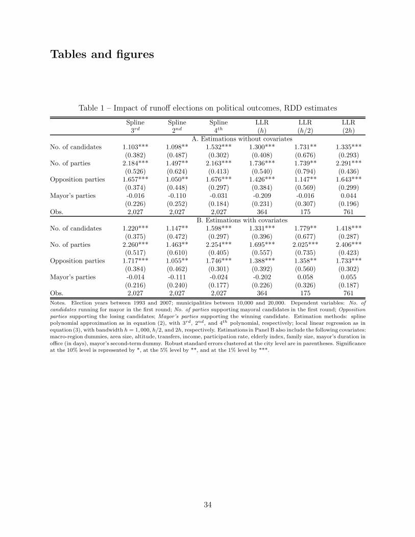
Tables and figures

Table 1 – Impact of runoff elections on political outcomes, RDD estimates

Spline Spline Spline LLR LLR LLR3rd 2nd 4th (h) (h/2) (2h)

A. Estimations without covariatesNo. of candidates 1.103*** 1.098** 1.532*** 1.300*** 1.731** 1.335***

(0.382) (0.487) (0.302) (0.408) (0.676) (0.293)No. of parties 2.184*** 1.497** 2.163*** 1.736*** 1.739** 2.291***

(0.526) (0.624) (0.413) (0.540) (0.794) (0.436)Opposition parties 1.657*** 1.050** 1.676*** 1.426*** 1.147** 1.643***

(0.374) (0.448) (0.297) (0.384) (0.569) (0.299)Mayor’s parties -0.016 -0.110 -0.031 -0.209 -0.016 0.044

(0.226) (0.252) (0.184) (0.231) (0.307) (0.196)Obs. 2,027 2,027 2,027 364 175 761

B. Estimations with covariatesNo. of candidates 1.220*** 1.147** 1.598*** 1.331*** 1.779** 1.418***

(0.375) (0.472) (0.297) (0.396) (0.677) (0.287)No. of parties 2.260*** 1.463** 2.254*** 1.695*** 2.025*** 2.406***

(0.517) (0.610) (0.405) (0.557) (0.735) (0.423)Opposition parties 1.717*** 1.055** 1.746*** 1.388*** 1.358** 1.733***

(0.384) (0.462) (0.301) (0.392) (0.560) (0.302)Mayor’s parties -0.014 -0.111 -0.024 -0.202 0.058 0.055

(0.216) (0.240) (0.177) (0.226) (0.326) (0.187)Obs. 2,027 2,027 2,027 364 175 761

Notes. Election years between 1993 and 2007; municipalities between 10,000 and 20,000. Dependent variables: No. of

candidates running for mayor in the first round; No. of parties supporting mayoral candidates in the first round; Opposition

parties supporting the losing candidates; Mayor’s parties supporting the winning candidate. Estimation methods: splinepolynomial approximation as in equation (2), with 3rd, 2nd, and 4th polynomial, respectively; local linear regression as in

equation (3), with bandwidth h = 1,000, h/2, and 2h, respectively. Estimations in Panel B also include the following covariates:macro-region dummies, area size, altitude, transfers, income, participation rate, elderly index, family size, mayor’s duration in

office (in days), mayor’s second-term dummy. Robust standard errors clustered at the city level are in parentheses. Significanceat the 10% level is represented by *, at the 5% level by **, and at the 1% level by ***.

34

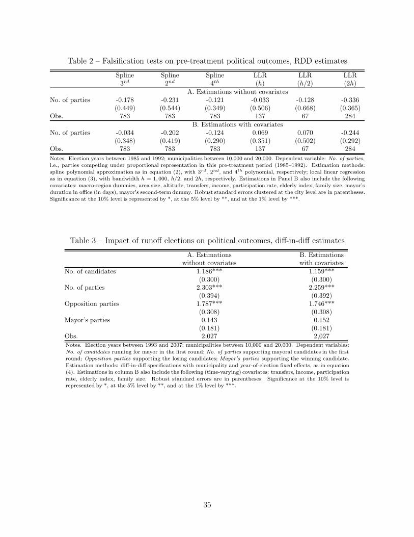
Table 2 – Falsification tests on pre-treatment political outcomes, RDD estimates

Spline Spline Spline LLR LLR LLR3rd 2nd 4th (h) (h/2) (2h)

A. Estimations without covariatesNo. of parties -0.178 -0.231 -0.121 -0.033 -0.128 -0.336

(0.449) (0.544) (0.349) (0.506) (0.668) (0.365)Obs. 783 783 783 137 67 284

B. Estimations with covariatesNo. of parties -0.034 -0.202 -0.124 0.069 0.070 -0.244

(0.348) (0.419) (0.290) (0.351) (0.502) (0.292)Obs. 783 783 783 137 67 284

Notes. Election years between 1985 and 1992; municipalities between 10,000 and 20,000. Dependent variable: No. of parties,i.e., parties competing under proportional representation in this pre-treatment period (1985–1992). Estimation methods:

spline polynomial approximation as in equation (2), with 3rd, 2nd, and 4th polynomial, respectively; local linear regressionas in equation (3), with bandwidth h = 1,000, h/2, and 2h, respectively. Estimations in Panel B also include the following

covariates: macro-region dummies, area size, altitude, transfers, income, participation rate, elderly index, family size, mayor’sduration in office (in days), mayor’s second-term dummy. Robust standard errors clustered at the city level are in parentheses.

Significance at the 10% level is represented by *, at the 5% level by **, and at the 1% level by ***.

Table 3 – Impact of runoff elections on political outcomes, diff-in-diff estimates

A. Estimations B. Estimationswithout covariates with covariates

No. of candidates 1.186*** 1.159***(0.300) (0.300)

No. of parties 2.303*** 2.259***(0.394) (0.392)

Opposition parties 1.787*** 1.746***(0.308) (0.308)

Mayor’s parties 0.143 0.152(0.181) (0.181)

Obs. 2,027 2,027

Notes. Election years between 1993 and 2007; municipalities between 10,000 and 20,000. Dependent variables:

No. of candidates running for mayor in the first round; No. of parties supporting mayoral candidates in the firstround; Opposition parties supporting the losing candidates; Mayor’s parties supporting the winning candidate.

Estimation methods: diff-in-diff specifications with municipality and year-of-election fixed effects, as in equation(4). Estimations in column B also include the following (time-varying) covariates: transfers, income, participation

rate, elderly index, family size. Robust standard errors are in parentheses. Significance at the 10% level isrepresented by *, at the 5% level by **, and at the 1% level by ***.

35

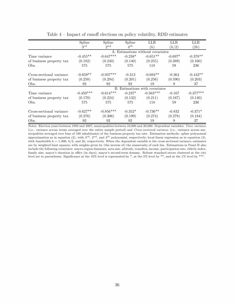
Table 4 – Impact of runoff elections on policy volatility, RDD estimates

Spline Spline Spline LLR LLR LLR3rd 2nd 4th (h) (h/2) (2h)

A. Estimations without covariatesTime variance -0.455** -0.647*** -0.238* -0.651** -0.697* -0.378**of business property tax (0.182) (0.240) (0.140) (0.255) (0.389) (0.160)Obs. 575 575 575 118 59 236

Cross-sectional variance -0.659** -0.937*** -0.313 -0.694** -0.364 -0.443**of business property tax (0.258) (0.294) (0.201) (0.256) (0.590) (0.203)Obs. 92 92 92 19 9 37

B. Estimations with covariatesTime variance -0.450*** -0.614*** -0.237* -0.563*** -0.167 -0.377***of business property tax (0.170) (0.224) (0.132) (0.211) (0.167) (0.140)Obs. 575 575 575 118 59 236

Cross-sectional variance -0.627** -0.856*** -0.352* -0.736** -0.832 -0.371*of business property tax (0.276) (0.306) (0.199) (0.274) (0.278) (0.184)Obs. 92 92 92 19 9 37

Notes. Election years between 1993 and 2007; municipalities between 10,000 and 20,000. Dependent variables: Time variance

(i.e., variance across terms averaged over the entire sample period) and Cross-sectional variance (i.e., variance across mu-nicipalities averaged over bins of 100 inhabitants) of the business property tax rate. Estimation methods: spline polynomial

approximation as in equation (2), with 3rd, 2nd, and 4th polynomial, respectively; local linear regression as in equation (3),with bandwidth h = 1,000, h/2, and 2h, respectively. When the dependent variable is the cross-sectional variance, estimates

are by weighted least squares, with weights given by (the inverse of) the numerosity of each bin. Estimations in Panel B alsoinclude the following covariates: macro-region dummies, area size, altitude, transfers, income, participation rate, elderly index,

family size, mayor’s duration in office (in days), mayor’s second-term dummy. Robust standard errors clustered at the citylevel are in parentheses. Significance at the 10% level is represented by *, at the 5% level by **, and at the 1% level by ***.

36

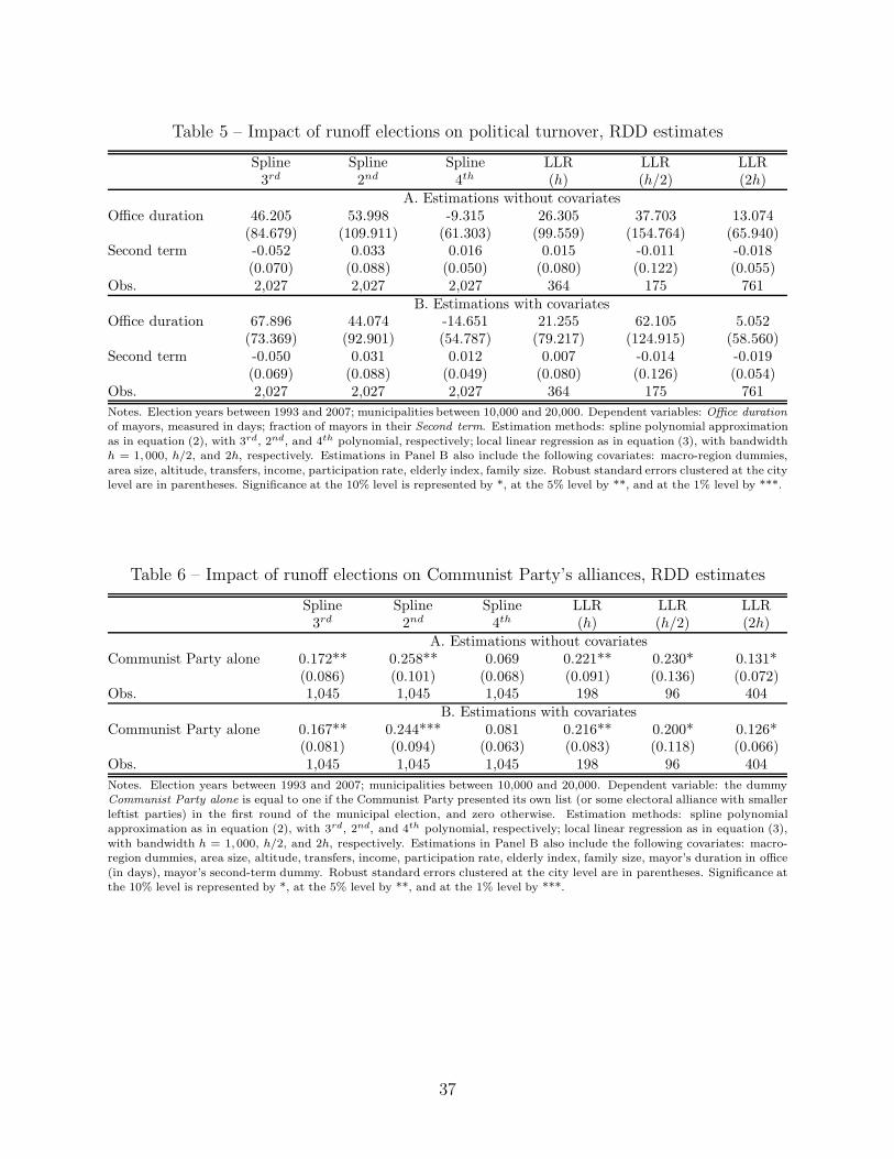
Table 5 – Impact of runoff elections on political turnover, RDD estimates

Spline Spline Spline LLR LLR LLR3rd 2nd 4th (h) (h/2) (2h)

A. Estimations without covariatesOffice duration 46.205 53.998 -9.315 26.305 37.703 13.074

(84.679) (109.911) (61.303) (99.559) (154.764) (65.940)Second term -0.052 0.033 0.016 0.015 -0.011 -0.018

(0.070) (0.088) (0.050) (0.080) (0.122) (0.055)Obs. 2,027 2,027 2,027 364 175 761

B. Estimations with covariatesOffice duration 67.896 44.074 -14.651 21.255 62.105 5.052

(73.369) (92.901) (54.787) (79.217) (124.915) (58.560)Second term -0.050 0.031 0.012 0.007 -0.014 -0.019

(0.069) (0.088) (0.049) (0.080) (0.126) (0.054)Obs. 2,027 2,027 2,027 364 175 761

Notes. Election years between 1993 and 2007; municipalities between 10,000 and 20,000. Dependent variables: Office duration

of mayors, measured in days; fraction of mayors in their Second term. Estimation methods: spline polynomial approximation

as in equation (2), with 3rd, 2nd, and 4th polynomial, respectively; local linear regression as in equation (3), with bandwidthh = 1,000, h/2, and 2h, respectively. Estimations in Panel B also include the following covariates: macro-region dummies,

area size, altitude, transfers, income, participation rate, elderly index, family size. Robust standard errors clustered at the citylevel are in parentheses. Significance at the 10% level is represented by *, at the 5% level by **, and at the 1% level by ***.

Table 6 – Impact of runoff elections on Communist Party’s alliances, RDD estimates

Spline Spline Spline LLR LLR LLR3rd 2nd 4th (h) (h/2) (2h)

A. Estimations without covariatesCommunist Party alone 0.172** 0.258** 0.069 0.221** 0.230* 0.131*

(0.086) (0.101) (0.068) (0.091) (0.136) (0.072)Obs. 1,045 1,045 1,045 198 96 404

B. Estimations with covariatesCommunist Party alone 0.167** 0.244*** 0.081 0.216** 0.200* 0.126*

(0.081) (0.094) (0.063) (0.083) (0.118) (0.066)Obs. 1,045 1,045 1,045 198 96 404

Notes. Election years between 1993 and 2007; municipalities between 10,000 and 20,000. Dependent variable: the dummyCommunist Party alone is equal to one if the Communist Party presented its own list (or some electoral alliance with smaller

leftist parties) in the first round of the municipal election, and zero otherwise. Estimation methods: spline polynomialapproximation as in equation (2), with 3rd, 2nd, and 4th polynomial, respectively; local linear regression as in equation (3),

with bandwidth h = 1,000, h/2, and 2h, respectively. Estimations in Panel B also include the following covariates: macro-region dummies, area size, altitude, transfers, income, participation rate, elderly index, family size, mayor’s duration in office

(in days), mayor’s second-term dummy. Robust standard errors clustered at the city level are in parentheses. Significance atthe 10% level is represented by *, at the 5% level by **, and at the 1% level by ***.

37

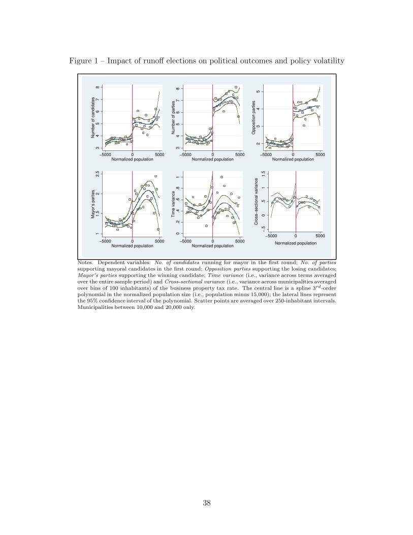
Figure 1 – Impact of runoff elections on political outcomes and policy volatility

34

56

78

Nu

mb

er

of

ca

nd

ida

tes

−5000 0 5000Normalized population

34

56

78

Nu

mb

er

of

pa

rtie

s

−5000 0 5000Normalized population

23

45

Op

po

sitio

n p

art

ies

−5000 0 5000Normalized population

11

.52

2.5

Ma

yo

r’s p

art

ies

−5000 0 5000Normalized population

0.2

.4.6

.81

Tim

e v

aria

nce

−5000 0 5000Normalized population

−.5

0.5

11

.5

Cro

ss−

se

ctio

na

l va

ria

nce

−5000 0 5000

Normalized population

Notes. Dependent variables: No. of candidates running for mayor in the first round; No. of parties

supporting mayoral candidates in the first round; Opposition parties supporting the losing candidates;Mayor’s parties supporting the winning candidate; Time variance (i.e., variance across terms averagedover the entire sample period) and Cross-sectional variance (i.e., variance across municipalities averagedover bins of 100 inhabitants) of the business property tax rate. The central line is a spline 3rd-orderpolynomial in the normalized population size (i.e., population minus 15,000); the lateral lines representthe 95% confidence interval of the polynomial. Scatter points are averaged over 250-inhabitant intervals.Municipalities between 10,000 and 20,000 only.

38

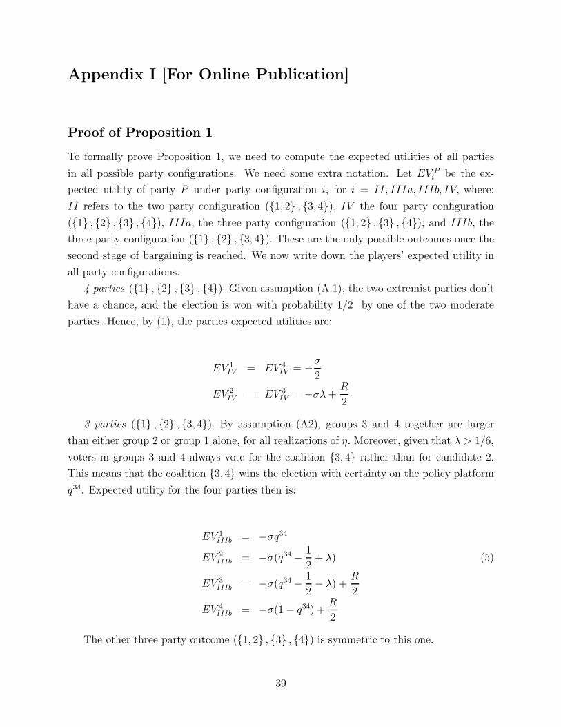
Appendix I [For Online Publication]

Proof of Proposition 1

To formally prove Proposition 1, we need to compute the expected utilities of all parties

in all possible party configurations. We need some extra notation. Let EV Pi be the ex-

pected utility of party P under party configuration i, for i = II, IIIa, IIIb, IV, where:

II refers to the two party configuration ({1, 2} , {3, 4}), IV the four party configuration

({1} , {2} , {3} , {4}), IIIa, the three party configuration ({1, 2} , {3} , {4}); and IIIb, the

three party configuration ({1} , {2} , {3, 4}). These are the only possible outcomes once the

second stage of bargaining is reached. We now write down the players’ expected utility in

all party configurations.

4 parties ({1} , {2} , {3} , {4}). Given assumption (A.1), the two extremist parties don’t

have a chance, and the election is won with probability 1/2 by one of the two moderate

parties. Hence, by (1), the parties expected utilities are:

EV 1IV = EV 4

IV = −σ

2

EV 2IV = EV 3

IV = −σλ +R

2

3 parties ({1} , {2} , {3, 4}). By assumption (A2), groups 3 and 4 together are larger

than either group 2 or group 1 alone, for all realizations of η. Moreover, given that λ > 1/6,

voters in groups 3 and 4 always vote for the coalition {3, 4} rather than for candidate 2.

This means that the coalition {3, 4} wins the election with certainty on the policy platform

q34. Expected utility for the four parties then is:

EV 1IIIb = −σq34

EV 2IIIb = −σ(q34 −

1

2+ λ) (5)

EV 3IIIb = −σ(q34 −

1

2− λ) +

R

2

EV 4IIIb = −σ(1 − q34) +

R

2

The other three party outcome ({1, 2} , {3} , {4}) is symmetric to this one.

39

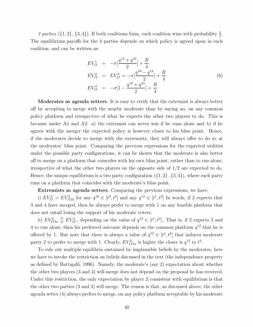
2 parties ({1, 2} , {3, 4}). If both coalitions form, each coalition wins with probability 12.

The equilibrium payoffs for the 4 parties depends on which policy is agreed upon in each

coalition, and can be written as:

EV 1II = −σ[

q12 + q34

2] +

R

4

EV 2II = EV 3

II = −σ[q34 − q12

2] +

R

4(6)

EV 4II = −σ[1−

q12 + q34

2] +

R

4

Moderates as agenda setters. It is easy to verify that the extremist is always better

off by accepting to merge with the nearby moderate than by saying no, on any common

policy platform and irrespective of what he expects the other two players to do. This is

because under A1 and A2: a) the extremist can never win if he runs alone and b) if he

agrees with the merger the expected policy is however closer to his bliss point. Hence,

if the moderates decide to merge with the extremists, they will always offer to do so at

the moderates’ bliss point. Comparing the previous expressions for the expected utilities

under the possible party configurations, it can be shown that the moderate is also better

off to merge on a platform that coincides with his own bliss point, rather than to run alone,

irrespective of what the other two players on the opposite side of 1/2 are expected to do.

Hence, the unique equilibrium is a two party configuration ({1, 2} , {3, 4}), where each party

runs on a platform that coincides with the moderate’s bliss point.

Extremists as agenda setters. Comparing the previous expressions, we have:

i) EV 2II > EV 2

IIIb for any q34 ∈ [t3, t4] and any q12 ∈ [t1, t2] In words, if 2 expects that

3 and 4 have merged, then he always prefer to merge with 1 on any feasible platform that

does not entail losing the support of his moderate voters.

ii) EV 2IIIa R EV 4

IV , depending on the value of q12 ∈ [t1, t2]. That is, if 2 expects 3 and

4 to run alone, then his preferred outcome depends on the common platform q12 that he is

offered by 1. But note that there is always a value of q12 ∈ [t1, t2] that induces moderate

party 2 to prefer to merge with 1. Clearly, EV 2IIIa is higher the closer is q12 to t2.

To rule out multiple equilibria sustained by implausible beliefs by the moderates, here

we have to invoke the restriction on beliefs discussed in the text (the independence property

as defined by Battigalli, 1996). Namely, the moderate’s (say 2) expectation about whether

the other two players (3 and 4) will merge does not depend on the proposal he has received.

Under this restriction, the only expectation by player 2 consistent with equilibrium is that

the other two parties (3 and 4) will merge. The reason is that, as discussed above, the other

agenda setter (4) always prefers to merge, on any policy platform acceptable by his moderate

40

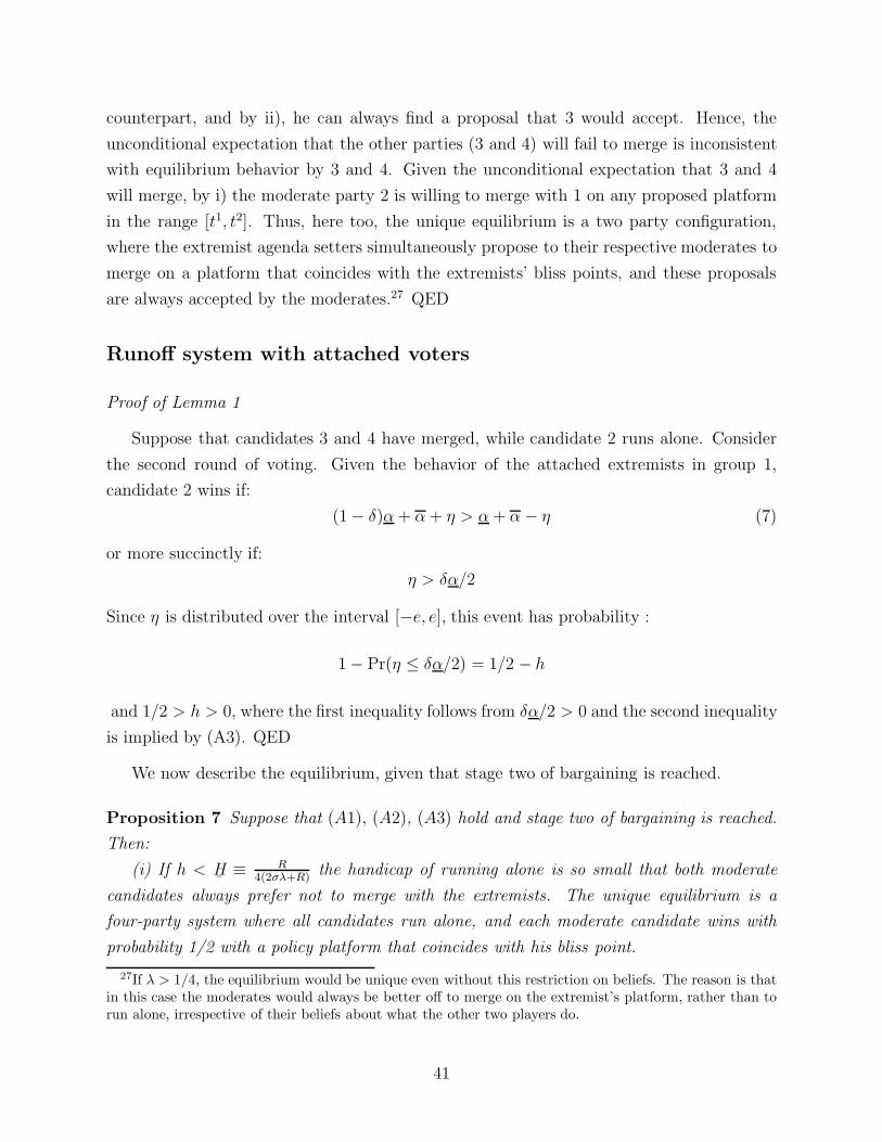
counterpart, and by ii), he can always find a proposal that 3 would accept. Hence, the

unconditional expectation that the other parties (3 and 4) will fail to merge is inconsistent

with equilibrium behavior by 3 and 4. Given the unconditional expectation that 3 and 4

will merge, by i) the moderate party 2 is willing to merge with 1 on any proposed platform

in the range [t1, t2]. Thus, here too, the unique equilibrium is a two party configuration,

where the extremist agenda setters simultaneously propose to their respective moderates to

merge on a platform that coincides with the extremists’ bliss points, and these proposals

are always accepted by the moderates.27 QED

Runoff system with attached voters

Proof of Lemma 1

Suppose that candidates 3 and 4 have merged, while candidate 2 runs alone. Consider

the second round of voting. Given the behavior of the attached extremists in group 1,

candidate 2 wins if:

(1 − δ)α + α + η > α + α − η (7)

or more succinctly if:

η > δα/2

Since η is distributed over the interval [−e, e], this event has probability :

1 − Pr(η ≤ δα/2) = 1/2 − h

and 1/2 > h > 0, where the first inequality follows from δα/2 > 0 and the second inequality

is implied by (A3). QED

We now describe the equilibrium, given that stage two of bargaining is reached.

Proposition 7 Suppose that (A1), (A2), (A3) hold and stage two of bargaining is reached.

Then:

(i) If h < H¯

≡ R4(2σλ+R)

the handicap of running alone is so small that both moderate

candidates always prefer not to merge with the extremists. The unique equilibrium is a

four-party system where all candidates run alone, and each moderate candidate wins with

probability 1/2 with a policy platform that coincides with his bliss point.

27If λ > 1/4, the equilibrium would be unique even without this restriction on beliefs. The reason is thatin this case the moderates would always be better off to merge on the extremist’s platform, rather than torun alone, irrespective of their beliefs about what the other two players do.

41

(ii) If h > H ≡ R4(2σλ+R/2)

, the handicap of running alone is so large that both moderate

candidates always prefer to merge with the extremists. The unique equilibrium is a two

party system where moderates and extremists merge on both sides and each party wins with

probability 1/2. If the moderate candidate is the agenda setter, then the policy platforms

of each coalition coincide with the moderates’ bliss points. If the extremist candidate is the

agenda setter, then the policy platforms of each coalition lie in between the extremist and

the moderate bliss points, and the distance between the equilibrium policy platforms and the

moderates’ bliss points is (weakly) decreasing in h.

(iii) If H¯

≤ h ≤ H, then two equilibria are possible. Depending on the players’ expecta-

tions about what the other candidates are doing, both a two party or a four party system can

emerge in equilibrium. In a two party system, the policy platforms are as described under

point (ii).

Proof of Proposition 7

Moderates as agenda setters. Suppose first that the moderate candidates are the

agenda setter inside each prospective coalition. Consider candidate 2, given that 3 and 4

have merged. If candidate 2 runs alone, as explained in the text, he wins with probability

1/2 − h. If he wins, he implements his bliss point and enjoys the rents from office, R. If he

loses, he gets no rents and the policy implemented is t3 = 1/2 + λ. Hence, using the same

notation as in the proof of Proposition 1, candidate 2’s expected utility when running alone

and given that 3 and 4 have merged is:

EV 2IIIb = (

1

2− h)R − 2σλ(

1

2+ h)

If instead candidate 2 merges with 1 and implements its preferred policy, then their

party wins with probability 1/2, but then candidate 2 has to share the rents from office

with the other party member. Hence, candidate 2’s expected utility when he merges with

1, given that 3 and 4 have merged is:

EV 2II = (

1

4)R − σλ

Comparing these two expressions, we see that 2 is indifferent between these two options

if

h = H¯

≡R

4(2σλ + R)(8)

Hence, if h < H¯

, candidate 2 prefers to run alone, given that 3 and 4 have merged, while if

h > H¯

, candidate 2 prefers to merge, given that 3 and 4 have merged.

42

Next, consider candidate 2’s alternatives if candidates 3 and 4 do not merge. If 2 also

runs alone, he wins with probability 1/2 and his expected utility is:

EV 2IV = −σλ +

R

2(9)

If instead candidate 2 merges with 1 and is the agenda setter inside his coalition, given that

3 and 4 have not merged, than party {1, 2} wins with probability (1 + h) and candidate 2’s

expected utility is:

EV 2IIIa = (

1

2+ h)

R

2− 2σλ(

1

2− h)

Comparing the last two expressions, we see that 2 is indifferent between the two options if

h = H ≡R

4(2σλ + R/2)(10)

For h < H, candidate 2 prefers to run alone, given that 3 and 4 have not merged; while for

h > H, 2 prefers to merge with 1, given that 3 and 4 have not merged and that 2 is the

agenda setter.

Comparing (8) and (10), we see that H >H¯

; running alone is more attractive (i.e., the

threshold of indifference is higher) if the opponents are also running alone. Hence, three

cases are possible, depending on parameter values:

If h < H¯, the handicap from running alone is so small that both moderate candidates

always prefer not to merge with the extremists. In this case, if the second stage of bargaining

is reached and the moderate candidates are drawn to be agenda setters, the equilibrium is

unique and we have a four party system.

If h > H, the handicap from running alone is so large that both moderate candidates

always prefer to merge with the extremists. In this case, if the second stage of bargaining

is reached and the moderate candidates are agenda setters, the equilibrium is again unique,

and we have a two party system on the moderates’ policy platforms.

Finally, if H¯

≤ h ≤ H, then multiple equilibria are possible, given that the second stage

of bargaining is reached and the moderate candidates are agenda setters. Depending on the

players’ expectations about what the other candidates are doing, we could have both a two

party or a four party system.

In all these cases, the policy platforms inside the coalitions coincide with those of the

moderate candidates since the extremists are always willing to merge.

Extremists as agenda setters. Next, suppose that extremist candidates are the

agenda setters. Let q34 ∈ [1/2 + λ, 1] denote the policy proposal for party {3, 4} and

43

q12 ∈ [0, 1/2−λ] the policy proposal for party {1, 2} . These policies need not coincide with

the extremist candidates bliss points, since the extremists may have to deviate from their

bliss points to get their proposals accepted. Our goal is to establish conditions under which

such proposals might or might not be accepted by the moderate candidates. Again, we focus

attention on candidate 2, under different expectations about what happens in the opposing

party, since the extremists are alway better off when they merge.

Suppose that candidate 2 expects party {3, 4} to be formed on the policy platform q34.

Going through the same steps as above, candidate 2’s expected utility if he rejects or accepts

candidate 1’s proposal of a platform q12 are respectively:

EV 2IIIb = (

1

2− h)R − σ(

1

2+ h)(q34 −

1

2+ λ)

EV 2II = (

1

4)R +

σ

2(q12 − q34)

Hence, candidate 2 is indifferent between these two alternatives for:

h = H(q12, q34) ≡σ(1

2− λ − q12) + R/2

2σ(q34 − 12

+ λ) + 2R(11)

Thus, if candidate 2 expect coalition 3,4 to be formed, he prefers to run alone (to merge) if

h < H(q12, q34) (if h > H(q12, q34)). Note that H(.) is strictly decreasing in both arguments.

Intuitively, as q12 increases it approaches candidate’s 2 bliss point and the merger becomes

more attractive; while as q34 increases it gets further away from candidate’s 2 bliss point,

and this too makes the merger more attractive for candidate 2 (since losing the election

would cause more disutility).

By symmetry, if two parties are formed, in equilibrium the policy platforms agreed upon

by each coalition must have the same distance from 1/2. Hence, H(q12, q34) can be rewritten

(with a slight abuse of notation) as:

HM(q) ≡σ(1

2− λ − q) + R/2

2σ(12

+ λ − q) + 2R(12)

for q ∈ [0, 1/2 − λ] and where the M superscript serves as a reminder that 2 expects his

opponents to merge. It is easy to see that H¯

≤ HM (q) for any q ∈ [0, 1/2 − λ], where the

first inequality is strict if q < 1/2 − λ and it holds with equality at q = 1/2 − λ. Moreover,

44

HMq (q) < 0. Thus, the function HM (q) reaches a maximum at q = 0, where

HM (0) =σ(1

2− λ) + R/2

2σ(12

+ λ) + 2R

The policy q = 0 is the point of most extreme symmetric extremism; at this choice, q12 and

q34 coincide with the extremist candidates bliss points, 0 and 1 respectively. In words, as

the policy q approved inside each coalition becomes symmetrically more extreme, a merger

becomes less attractive for the moderate candidates, given that they expect a symmetric

merger to be formed by their opponent. Hence, they will be more willing to run alone and

refuse the merger, even if they expect a merger to occur in the opposing coalition.

Suppose now that candidate 2 does not expect a merger to occur in coalition 3,4. If he

runs alone, either himself or the other moderate party wins with probability 12. Hence his

expected utility is the same as in (9) above.

If he instead accepts the offer from candidate 1 to form a coalition at policy q12, his

expected utility, given the expectation that the coalition 3,4 will not form, is:

EV 2IIIa = (

1

2+ h)

R

2− σ(

1

2+ h)(

1

2− λ − q12) − 2σλ(

1

2− h)

which is an increasing function of q12. Candidate 2 will then be indifferent between accepting

1’s offer or running alone, given his expectations on 3,4 , if:

h = HA(q) ≡σ(1

2− λ − q) + R/2

2σ(q − 12

+ 3λ) + R

for q ∈ [0, 1/2 − λ] and where the A superscript serves as a reminder that 2 expects his

opponents not to merge. Candidate 2 will then accept 1’s offer if h ≥ HA(q) and refuses it

if h < HA(q). Clearly, HAq (q) < 0 and H ≤ HA(q), with equality at q = 1

2− λ.

We are now ready to characterize the equilibrium if the extremists are agenda setters

and stage two of bargaining is reached. Specifically:

If h < H¯

, then there is no feasible offer by an extremist that can induce a moderate

candidate to merge with him, whatever the moderate’s expectations about the other coali-

tion. This can be seen by noting that, as discussed above, H¯

≤ HM (q), HA(q) for all

q ∈ [0, 1/2 − λ]. Hence, the unique equilibrium is a 4 party system with all candidates

running alone.

If h > H, then the moderate candidate, say candidate 2, always prefers to merge with the

extremist on at least some (though not necessarily all) feasible policy platforms, whatever his

expectations on the other coalition’s behavior. This can be seen by noting that HM (q) ≤ H

45

for at least some q ∈ [0, 1/2 − λ], and HA(q) = H at the point q = 1/2 − λ. By symmetry,

candidate 2 will rationally expect that the other coalition will always be formed. He would

then accept any offer q by candidate 1 such that h ≥ HM (q). Hence, the unique equilibrium

is a two party system where extremists and moderates merge on both sides.

The extremists candidates who act as agenda setters will then impose the policy plat-

forms closest to their bliss points, subject to getting their proposal accepted. Since HM (0) SH, the equilibrium platform in this case varies with the value of h. If h ≥ HM(0), then

both coalitions will form on the extremist candidates bliss points, 0 and 1 for coalitions

{1, 2} and {3, 4} respectively. If h < HM (0), then coalition {1, 2} will form on the policy

q∗ ∈ [0, 1/2 − λ] such that h = HM(q∗), while coalition {3, 4} will form on the symmetric

policy 1 − q∗. This can seen by noting that any policy q′ < q∗ would not be accepted by

candidate 2 (since by (11) h < H(q′, q∗)), and any policy q′′ > q∗ would be accepted by

candidate 2 (since by (11) h > H(q′′, q∗)) but suboptimal for candidate 1 who is the agenda

setter. Since HMq (q) < 0, we have that ∂q∗

∂h= 1

HMq

≤ 0, with strict inequality if h < HM (0).

Thus, as h rises the equilibrium policy falls towards the extremists bliss point (or it remains

constant if it is already at the extremist’s bliss point).

Finally, if H¯

≤ h ≤ H, then two equilibrium outcomes are possible in pure strategies.

(i) If the moderate candidate expects his moderate opponent to run alone, he also prefers

to run alone (since h ≤ H ≤ HA(q)). Hence we have a four party equilibrium.(ii) If the

moderate candidate expects his opponents to merge, then he also prefers to merge rather

than running alone (since H = HM (1/2 − λ) ≤ HM (q) ≤ h for at least some q). Going

through the argument in previous paragraph, the equilibrium policy platform in this case

coincides with the extremist’s bliss point if h ≥ HM(0), and it is q∗ such that h = HM (q∗)

if h < HM (0). (Again, recall that HM (0) S H, depending on parameter values). QED

Finally, consider stage 1 of bargaining. As before, the equilibrium depends on how

polarized is the electorate. If voters are very polarized (if 1/2 ≥ λ > 1/4), then there is

no policy in the interval [t2, t3] that would command the support of all moderate voters.

Hence, the centrist party {2, 3} would lose the election with certainty, and both moderates

prefer to move to the second stage of the bargaining game. Hence, if 1/2 ≥ λ > 1/4 the

final equilibrium is as described in Proposition 7.

Suppose instead that 1/4 ≥ λ > 1/6. Here the centrist party would win for sure for

a range of policy platforms. But this needs not imply that the centrist party is formed,

because such a party would still have to reach a policy compromise and dilute rents among

coalition members. If the handicap from running alone is sufficiently small (if h < H¯

),

then both moderate candidates know that the four party system emerges out of the second

stage game (see Proposition 7). Hence, by linearity of payoffs, they are exactly indifferent

46

between forming the centrist party with a policy platform of q = 1/2 or running alone in

a four party system. A slight degree of risk aversion would push them towards the centrist

party, but an extra dilution of rents in a coalition government compared to the expected

rents if they run alone would push them in the opposite direction. If instead the handicap

from running alone is sufficiently large (h > H), then the moderates are strictly better off

with the centrist party, since the continuation game would lead them to merge with the

extremists. Finally, for intermediate values of the handicap (if H¯

≤ h ≤ H), both outcomes

are possible, depending on players beliefs about continuation equilibrium. Thus we have:

Proposition 8 Suppose that (A1), (A2), (A3) hold.

(i) If 1/2 ≥ λ > 1/4, then the unique equilibrium outcome under dual ballot is as

described in Proposition 7.

(ii) If 1/4 ≥ λ > 1/6 and h > H, then the unique equilibrium outcome under dual ballot

is a three party system with a centrist party, ({1} , {2, 3} , {4}). The centrist party wins the

election with certainty, and implements the policy platform q = 1/2.

(iii) If 1/4 ≥ λ > 1/6 and h ≤ H, then two equilibrium outcomes are possible under

dual ballot: either the three party system with a centrist party described above, or the four

party system described in part (i) of Proposition 7.

Equilibrium with endorsements

Suppose that both moderate candidates have passed the first round. Define

ε ≡δα

2(1 +

4σλ

R) −

e

2≷ 0

We have:

Lemma 2 Irrespective of what candidate 3 does, candidate 2 prefers to be endorsed by

the extremist if ε1 < ε, and he prefers no endorsement if ε1 > ε + δα2. In between, if

ε ≤ ε1 ≤ ε + δα2, then 2 prefers to seek the endorsement of the extremist if 3 has also been

endorsed, while 2 prefers no endorsement if 3 has not been endorsed. Candidate 3 behaves

symmetrically (in the opposite direction), depending on whether −ε1 is below or above these

same thresholds.

Proof of Lemma 2

Suppose that both 2 and 3 have been endorsed by their extremist neighbors. By our

previous assumptions, candidate 2 wins if ε1 + ε2 > 0. When decisions over endorsements

are made, the realization of ε1 is known, but ε2 is not. Hence the probability that candidate

47

2 wins is

Pr(ε2 > −ε1) =1

2+

ε1

e(13)

where the right hand side follows from (2). Candidate 2’s expected utility is:

(1

2+

ε1

e)R

2− 2σλ(

1

2−

ε1

e) (14)

Suppose instead that 3 has been endorsed by 4 while 2 did not seek the endorsement of

1. Now 2 loses the support of δα voters, the attached extremists in group 1, while 3 carries

all voters in group 4. Hence, repeating the analysis in (7), the probability that 2 wins is:

Pr(ε2 >δα

2− ε1) =

1

2+

ε1

e−

δα

2e(15)

if ε1 ≥δα2− e

2, and it is 0 if ε1 < δα

2− e

2. Candidate 2’s expected utility is:

(1

2+

ε1

e−

δα

2e)R − 2σλ(

1

2−

ε1

e+

δα

2e)

provided that the first expression in brackets is strictly positive and the second expression

in brackets is stricly less than 1, which occurs if ε1 ≥δα2− e

2. If instead ε1 < − e

2+ δα

2, then

the probability that 2 wins is 0 and his expected utility reduces to −2σλ.28

Candidate 2 is indifferent between these two alternatives if:

ε1 = ε ≡δα

2(1 +

4σλ

R) −

e

2(16)

If ε1 > ε then candidate 2 strictly prefers no endorsement, given that 3 has not been

endorsed. While if ε1 < ε then candidate 2 strictly prefers to be endorsed, given that 3 has

not been endorsed.

Next, suppose that both moderate candidates have been endorsed by the extremist. By

symmetry, the probability that 2 wins is still descibed by (13). Candidate 2’s expected

utility if no candidate is endorsed is thus:

(1

2+

ε1

e)R − 2σλ(

1

2−

ε1

e)

If instead candidate 2 has been endorsed and 3 has not, the probability that 2 wins is:

Pr(ε2 > −δα

2− ε1) =

1

2+

ε1

e+

δα

2e(17)

28By (A3), the first expression in brackets is always strictly less than 1 and the second expression inbrackets is always positive.

48

if ε1 ≤e2− δα

2and it is 1 if ε1 > e

2− δα

2.29 In this case, candidate 2’s expected utility is:

(1

2+

ε1

e+

δα

2e)R

2− 2σλ(

1

2−

ε1

e−

δα

2e)

provided that the first expression in brackets is strictly less than 1 and the second expression

in brackets is stricly positive, which occurs if ε1 ≤e2− δα

2. If instead ε1 > e

2− δα

2, then the

probability that 2 wins is 1 and his expected utility reduces to R/2.30

Candidate 2 is then indifferent between these two options if

ε1 = ε +δα

2(18)

If ε1 > ε + δα2

then candidate 2 strictly prefers no endorsement, given that 3 has been

endorsed. While if ε1 < ε + δα2

then candidate 2 strictly prefers to be endorsed, given that

3 has been endorsed.

By symmetry, 3 has similar preferences, but in the opposite direction and with respect

to the symmetric thresholds −ε − δα2

and −ε (eg. 3 prefers no endorsement, given that 2

has been endorsed, if ε1 < −ε − δα2, and so on). QED

Finally, we describe the equilibrium continuation if the two moderate candidates have passed

the first round and compete over the second round. Equilibrium endorsements depend on

whether the thresholds in Lemma 2 are positive or negative. Specifically, under (A1-A3),

we have:

Proposition 9 (i) Suppose that ε > 0. Then the equilibrium is unique and at least one

of the two moderate candidates always seeks the endorsement of his extremist neighbor. If

ε1 ∈ [−ε− δα2, ε+ δα

2] then both candidates seek the endorsement of their extremist neighbor.

If ε1 > ε + δα2

then 3 seeks the endorsement while 2 does not. If ε1 < −ε− δα2

then 2 seeks

the endorsement while 3 does not.

(ii) Suppose that ε + δα2

< 0. Then the equilibrium is again unique and at most one of

the two moderate candidates seeks an endorsement by his extremist neighbor. If ε1 ∈ [ε,−ε]

then no moderate candidate seeks the endorsement of the extremist. If ε1 > −ε, then 3 seeks

the endorsement of 4 while 2 seeks no endorsement. If ε1 < ε, then 2 seeks the endorsement

of 1 while 3 seeks no endorsement.

(iii) Suppose that ε + δα2

> 0 > ε. If ε1 ∈ [−ε, ε], then multiple equilibria are possible:

either both moderate candidates seek an endorsement by their closest extremist or none of

29By (A3), Pr(ε2 > δα

2− ε1) < 1 and Pr(ε2 > − δα

2− ε1) > 0 for any ε1 ∈ [−e/2, e/2].

30Assumption (A3) implies that the first expression in brackets is always positive and the second one isalways less than 1.

49

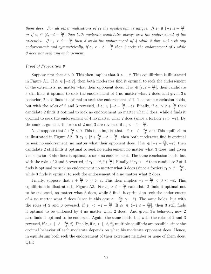
them does. For all other realizations of ε1 the equilibrium is unique. If ε1 ∈ (−ε, ε + δα2

]

or if ε1 ∈ (ε,−ε − δα2

] then both moderate candidates always seek the endorsement of the

extremist. If ε1 > ε + δα2

then 3 seeks the endorsement of 4 while 2 does not seek any

endorsement; and symmetrically, if ε1 < −ε − δα2

then 2 seeks the endorsement of 1 while

3 does not seek any endorsement.

Proof of Proposition 9

Suppose first that ε > 0. This then implies that 0 > − ε. This equilibrium is illustrated

in Figure A1. If ε1 ∈ [−ε, ε], then both moderates find it optimal to seek the endorsement

of the extremists, no matter what their opponent does. If ε1 ∈ (ε, ε + δα2

], then candidate

3 still finds it optimal to seek the endorsement of 4 no matter what 2 does; and given 3’s

behavior, 2 also finds it optimal to seek the endorsement of 1. The same conclusion holds,

but with the roles of 2 and 3 reversed, if ε1 ∈ [−ε − δα2

,−ε). Finally, if ε1 > ε + δα2

then

candidate 2 finds it optimal to seek no endorsement no matter what 3 does, while 3 finds it

optimal to seek the endorsement of 4 no matter what 2 does (since a fortiori ε1 > −ε). By

the same argument, the roles of 2 and 3 are reversed if ε1 < −ε− δα2

.

Next suppose that ε+ δα2

< 0. This then implies that −ε > −ε− δα2

> 0. This equilibrium

is illustrated in Figure A2. If ε1 ∈ [ε + δα2

,−ε − δα2

], then both moderates find it optimal

to seek no endorsement, no matter what their opponent does. If ε1 ∈ [−ε − δα2,−ε), then

candidate 2 still finds it optimal to seek no endorsement no matter what 3 does; and given

2’s behavior, 3 also finds it optimal to seek no endorsement. The same conclusion holds, but

with the roles of 2 and 3 reversed, if ε1 ∈ (ε, ε+ δα2

]. Finally, if ε1 > −ε then candidate 2 still

finds it optimal to seek no endorsement no matter what 3 does (since a fortiori ε1 > ε+ δα2

),

while 3 finds it optimal to seek the endorsement of 4 no matter what 2 does.

Finally, suppose that ε + δα2

> 0 > ε. This then implies −ε − δα2

< 0 < −ε. This

equilibrium is illustrated in Figure A3. For ε1 > ε + δα2

candidate 2 finds it optimal not

to be endorsed, no matter what 3 does, while 3 finds it optimal to seek the endorsement

of 4 no matter what 2 does (since in this case ε + δα2

> −ε). The same holds, but with

the roles of 2 and 3 reversed, if ε1 < −ε − δα2. If ε1 ∈ (−ε, ε + δα

2], then 3 still finds

it optimal to be endorsed by 4 no matter what 2 does. And given 3’s behavior, now 2

also finds it optimal to be endorsed. Again, the same holds, but with the roles of 2 and 3

reversed, if ε1 ∈ [−ε− δα2, ε). Finally, if ε1 ∈ [−ε, ε], multiple equilibria are possible, since the

optimal behavior of each moderate depends on what his moderate opponent does. Hence,

in equilibrium both seek the endorsement of their extremist neighbor or none of them does.

QED

50

Moderates as the smaller parties

Finally, we discuss a further extension of our model. The assumption that there are more

moderate than extremist voters is in line with the distribution of ideological preferences

observed in most countries. Nevertheless, the assumption plays a crucial role in the deriva-

tion of the result on policy moderation under the dual ballot. This section briefly discusses

whether the result on policy moderation survives under alternative assumptions about the

relative size of extremists vs moderate voters.

Although anything can happen under very general assumptions on the distribution of

voters’ preferences, there remains a reason why the dual ballot can induce policy moderation

even if the moderate groups are smaller than the extremists. Moderates have an option that

the extremists do not have: they can bargain with each other over the formation of a centrist

party. The runoff system can strengthen the incentives for the emergence of a centrist party,

and in this way it can induce more policy moderation. The basic reason is that under runoff

what matters is not to win the first round, but to pass it and and to win the final elections.

And a centrist party that manages to pass the first round has a larger probability to win

the final elections, as it can then collect the voters of the excluded extremist party.31

To illustrate this point, consider the following version of the model. Suppose that mod-

erates have size α and extremists size α, with α < α, exactly the reverse of what we assumed

in Section 2. Suppose further that the shock η = ε1 + ε2 changes the relative size of the two

larger groups, now the extremists, in the same symmetric way described in Section 2. The

size of the two centrist groups remains fixed at α. Everything else is kept unchanged, in-

cluding the distribution of the shock, assumptions (A1-A3), and the sequence of bargaining.

So, moderates first bargain among them and then (possibly) with the extremists, according

to the rules described above. But we add a further assumption, namely:

e

2> (α − 2α) > 0 (A4)

The second inequality implies that a single extremist group is larger (in expected value)

than the sum of the two moderates. The first inequality implies that, at each ballot, electoral

uncertainty is large enough to modify this ranking for some realization of the shock.32 We

also assume that 1/4 ≥ λ > 1/6, so that a viable centrist party is feasible (there exists a

centrist policy platform which would be preferred by all moderate voters to the extremist

bliss points). Consider then again the two electoral rules.

31In a different modeling context, the same intuition explains the result of greater moderation of policyunder the dual ballot system in Osborne and Slivinski (2001).

32Assumption (A4) is consistent with (A1-A2) if α/2 > α > α/3.

51

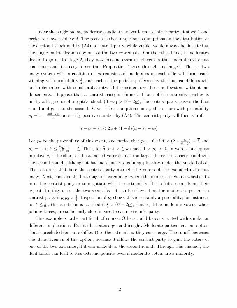
Under the single ballot, moderate candidates never form a centrist party at stage 1 and

prefer to move to stage 2. The reason is that, under our assumptions on the distribution of

the electoral shock and by (A4), a centrist party, while viable, would always be defeated at

the single ballot elections by one of the two extremists. On the other hand, if moderates

decide to go on to stage 2, they now become essential players in the moderate-extremist

coalitions, and it is easy to see that Proposition 1 goes through unchanged. Thus, a two

party system with a coalition of extremists and moderates on each side will form, each

winning with probability 12, and each of the policies preferred by the four candidates will

be implemented with equal probability. But consider now the runoff system without en-

dorsements. Suppose that a centrist party is formed. If one of the extremist parties is

hit by a large enough negative shock (if −ε1 > α − 2α), the centrist party passes the first

round and goes to the second. Given the assumptions on ε1, this occurs with probability

p1 = 1 − 2(α−2α)e

, a strictly positive number by (A4). The centrist party will then win if:

α + ε1 + ε2 < 2α + (1 − δ)(α − ε1 − ε2)

Let p2 be the probability of this event, and notice that p2 = 0, if δ ≥ (2 − αα+ e

4

) ≡ δ and

p2 = 1, if δ ≤ 2(α−e)(α−e)

≡ δ. Thus, for δ > δ > δ we have 1 > p2 > 0. In words, and quite

intuitively, if the share of the attached voters is not too large, the centrist party could win

the second round, although it had no chance of gaining plurality under the single ballot.

The reason is that here the centrist party attracts the voters of the excluded extremist

party. Next, consider the first stage of bargaining, where the moderates choose whether to

form the centrist party or to negotiate with the extremists. This choice depends on their

expected utility under the two scenarios. It can be shown that the moderates prefer the

centrist party if p1p2 > 12. Inspection of p2 shows this is certainly a possibility; for instance,

for δ ≤ δ , this condition is satisfied if e4

> (α − 2α), that is, if the moderate voters, when

joining forces, are sufficiently close in size to each extremist party.

This example is rather artificial, of course. Others could be constructed with similar or

different implications. But it illustrates a general insight. Moderate parties have an option

that is precluded (or more difficult) to the extremists: they can merge. The runoff increases

the attractiveness of this option, because it allows the centrist party to gain the voters of

one of the two extremes, if it can make it to the second round. Through this channel, the

dual ballot can lead to less extreme policies even if moderate voters are a minority.

52

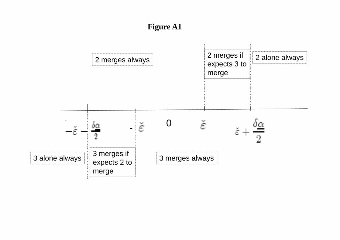
0-

Figure A1

3 merges always

2 alone always2 merges always 2 merges ifexpects 3 tomerge

3 alone always 3 merges ifexpects 2 tomerge

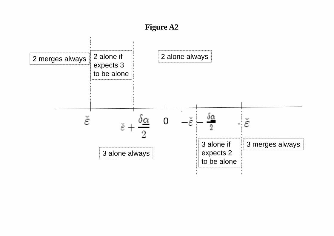
0 -

Figure A2

3 merges always

2 alone always2 merges always 2 alone ifexpects 3 to be alone

3 alone always3 alone ifexpects 2to be alone

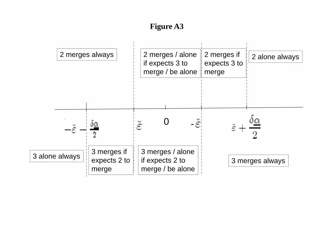
0 -

Figure A3

3 merges always

2 alone always2 merges always 2 merges ifexpects 3 tomerge

3 alone always 3 merges ifexpects 2 tomerge

2 merges / aloneif expects 3 tomerge / be alone

3 merges / aloneif expects 2 tomerge / be alone

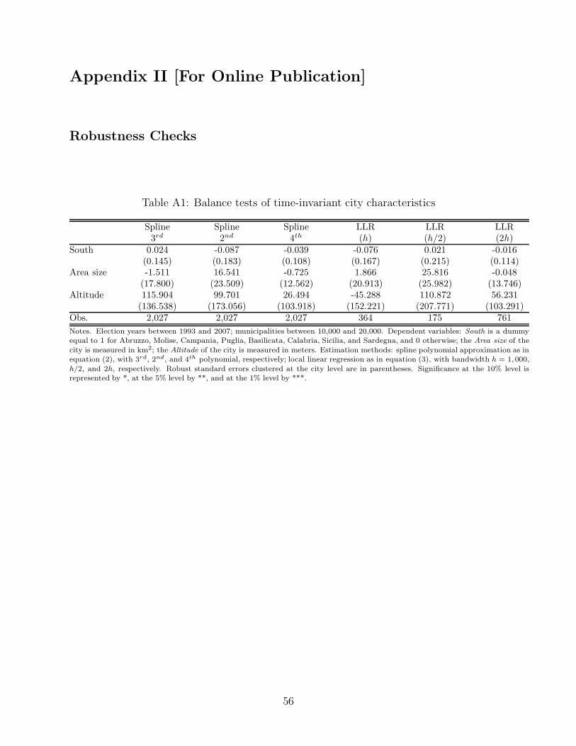
Appendix II [For Online Publication]

Robustness Checks

Table A1: Balance tests of time-invariant city characteristics

Spline Spline Spline LLR LLR LLR3rd 2nd 4th (h) (h/2) (2h)

South 0.024 -0.087 -0.039 -0.076 0.021 -0.016(0.145) (0.183) (0.108) (0.167) (0.215) (0.114)

Area size -1.511 16.541 -0.725 1.866 25.816 -0.048(17.800) (23.509) (12.562) (20.913) (25.982) (13.746)

Altitude 115.904 99.701 26.494 -45.288 110.872 56.231(136.538) (173.056) (103.918) (152.221) (207.771) (103.291)

Obs. 2,027 2,027 2,027 364 175 761

Notes. Election years between 1993 and 2007; municipalities between 10,000 and 20,000. Dependent variables: South is a dummyequal to 1 for Abruzzo, Molise, Campania, Puglia, Basilicata, Calabria, Sicilia, and Sardegna, and 0 otherwise; the Area size of the

city is measured in km2; the Altitude of the city is measured in meters. Estimation methods: spline polynomial approximation as inequation (2), with 3rd, 2nd, and 4th polynomial, respectively; local linear regression as in equation (3), with bandwidth h = 1,000,

h/2, and 2h, respectively. Robust standard errors clustered at the city level are in parentheses. Significance at the 10% level isrepresented by *, at the 5% level by **, and at the 1% level by ***.

56

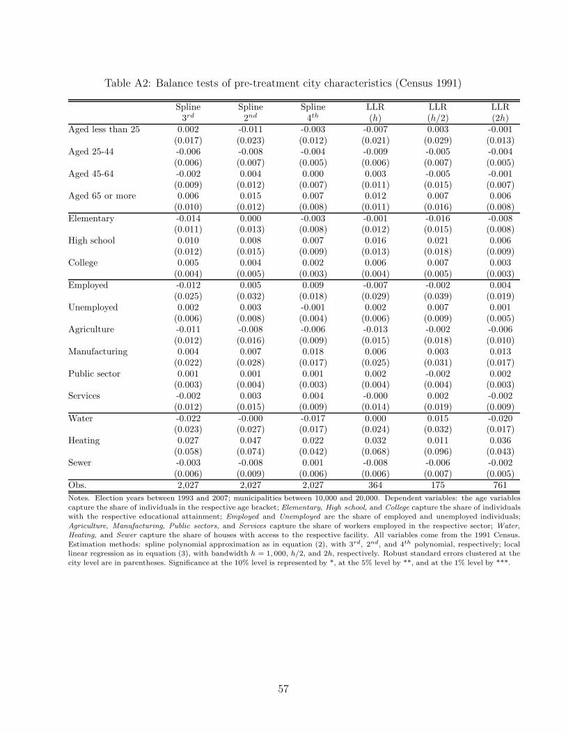
Table A2: Balance tests of pre-treatment city characteristics (Census 1991)

Spline Spline Spline LLR LLR LLR3rd 2nd 4th (h) (h/2) (2h)

Aged less than 25 0.002 -0.011 -0.003 -0.007 0.003 -0.001(0.017) (0.023) (0.012) (0.021) (0.029) (0.013)

Aged 25-44 -0.006 -0.008 -0.004 -0.009 -0.005 -0.004(0.006) (0.007) (0.005) (0.006) (0.007) (0.005)

Aged 45-64 -0.002 0.004 0.000 0.003 -0.005 -0.001(0.009) (0.012) (0.007) (0.011) (0.015) (0.007)

Aged 65 or more 0.006 0.015 0.007 0.012 0.007 0.006(0.010) (0.012) (0.008) (0.011) (0.016) (0.008)

Elementary -0.014 0.000 -0.003 -0.001 -0.016 -0.008(0.011) (0.013) (0.008) (0.012) (0.015) (0.008)

High school 0.010 0.008 0.007 0.016 0.021 0.006(0.012) (0.015) (0.009) (0.013) (0.018) (0.009)

College 0.005 0.004 0.002 0.006 0.007 0.003(0.004) (0.005) (0.003) (0.004) (0.005) (0.003)

Employed -0.012 0.005 0.009 -0.007 -0.002 0.004(0.025) (0.032) (0.018) (0.029) (0.039) (0.019)

Unemployed 0.002 0.003 -0.001 0.002 0.007 0.001(0.006) (0.008) (0.004) (0.006) (0.009) (0.005)

Agriculture -0.011 -0.008 -0.006 -0.013 -0.002 -0.006(0.012) (0.016) (0.009) (0.015) (0.018) (0.010)

Manufacturing 0.004 0.007 0.018 0.006 0.003 0.013(0.022) (0.028) (0.017) (0.025) (0.031) (0.017)

Public sector 0.001 0.001 0.001 0.002 -0.002 0.002(0.003) (0.004) (0.003) (0.004) (0.004) (0.003)

Services -0.002 0.003 0.004 -0.000 0.002 -0.002(0.012) (0.015) (0.009) (0.014) (0.019) (0.009)

Water -0.022 -0.000 -0.017 0.000 0.015 -0.020(0.023) (0.027) (0.017) (0.024) (0.032) (0.017)

Heating 0.027 0.047 0.022 0.032 0.011 0.036(0.058) (0.074) (0.042) (0.068) (0.096) (0.043)

Sewer -0.003 -0.008 0.001 -0.008 -0.006 -0.002(0.006) (0.009) (0.006) (0.006) (0.007) (0.005)

Obs. 2,027 2,027 2,027 364 175 761

Notes. Election years between 1993 and 2007; municipalities between 10,000 and 20,000. Dependent variables: the age variables

capture the share of individuals in the respective age bracket; Elementary, High school, and College capture the share of individualswith the respective educational attainment; Employed and Unemployed are the share of employed and unemployed individuals;

Agriculture, Manufacturing, Public sectors, and Services capture the share of workers employed in the respective sector; Water,Heating, and Sewer capture the share of houses with access to the respective facility. All variables come from the 1991 Census.

Estimation methods: spline polynomial approximation as in equation (2), with 3rd, 2nd, and 4th polynomial, respectively; locallinear regression as in equation (3), with bandwidth h = 1, 000, h/2, and 2h, respectively. Robust standard errors clustered at the

city level are in parentheses. Significance at the 10% level is represented by *, at the 5% level by **, and at the 1% level by ***.

57

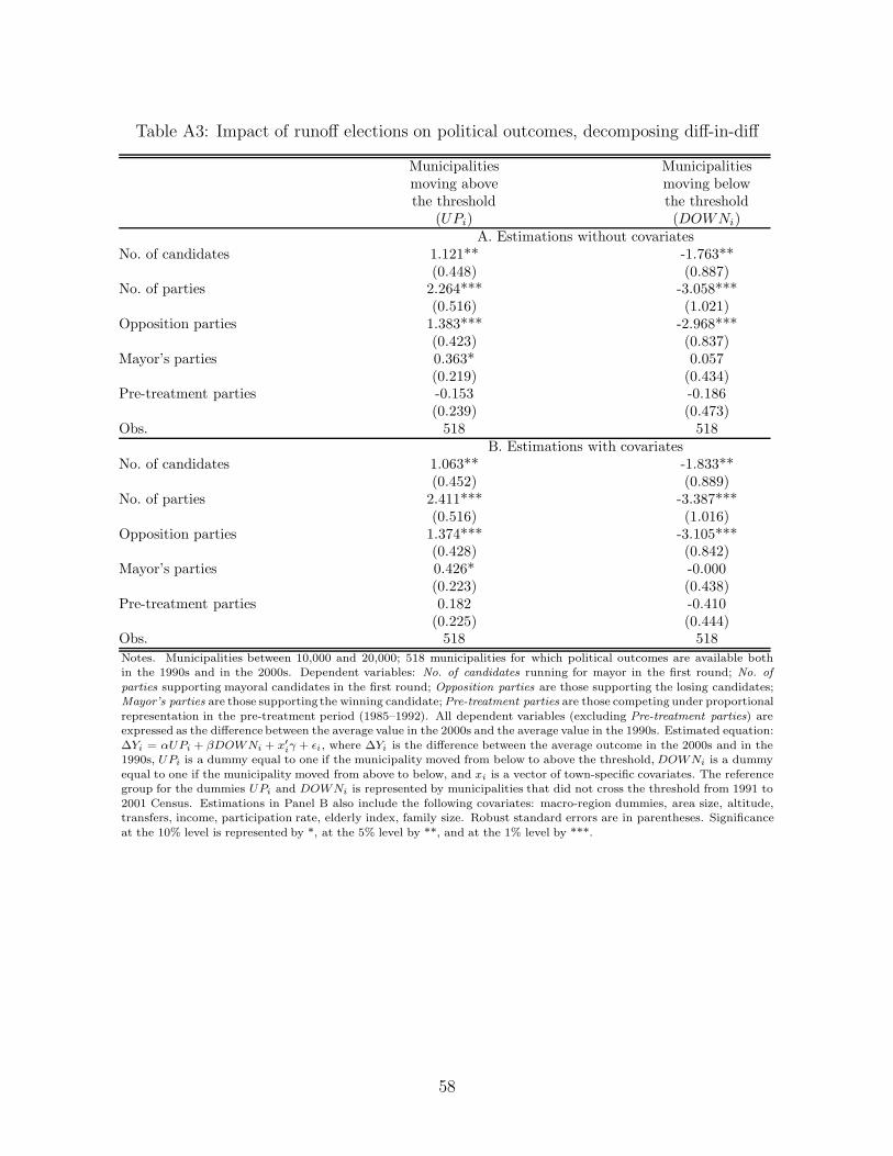
Table A3: Impact of runoff elections on political outcomes, decomposing diff-in-diff

Municipalities Municipalitiesmoving above moving belowthe threshold the threshold

(UPi) (DOWNi)A. Estimations without covariates

No. of candidates 1.121** -1.763**(0.448) (0.887)

No. of parties 2.264*** -3.058***(0.516) (1.021)

Opposition parties 1.383*** -2.968***(0.423) (0.837)

Mayor’s parties 0.363* 0.057(0.219) (0.434)

Pre-treatment parties -0.153 -0.186(0.239) (0.473)

Obs. 518 518B. Estimations with covariates

No. of candidates 1.063** -1.833**(0.452) (0.889)

No. of parties 2.411*** -3.387***(0.516) (1.016)

Opposition parties 1.374*** -3.105***(0.428) (0.842)

Mayor’s parties 0.426* -0.000(0.223) (0.438)

Pre-treatment parties 0.182 -0.410(0.225) (0.444)

Obs. 518 518

Notes. Municipalities between 10,000 and 20,000; 518 municipalities for which political outcomes are available bothin the 1990s and in the 2000s. Dependent variables: No. of candidates running for mayor in the first round; No. of

parties supporting mayoral candidates in the first round; Opposition parties are those supporting the losing candidates;Mayor’s parties are those supporting the winning candidate; Pre-treatment parties are those competing under proportional

representation in the pre-treatment period (1985–1992). All dependent variables (excluding Pre-treatment parties) areexpressed as the difference between the average value in the 2000s and the average value in the 1990s. Estimated equation:

∆Yi = αUPi + βDOWNi + x′

iγ + εi, where ∆Yi is the difference between the average outcome in the 2000s and in the1990s, UPi is a dummy equal to one if the municipality moved from below to above the threshold, DOWNi is a dummy

equal to one if the municipality moved from above to below, and xi is a vector of town-specific covariates. The referencegroup for the dummies UPi and DOWNi is represented by municipalities that did not cross the threshold from 1991 to

2001 Census. Estimations in Panel B also include the following covariates: macro-region dummies, area size, altitude,transfers, income, participation rate, elderly index, family size. Robust standard errors are in parentheses. Significance

at the 10% level is represented by *, at the 5% level by **, and at the 1% level by ***.

58

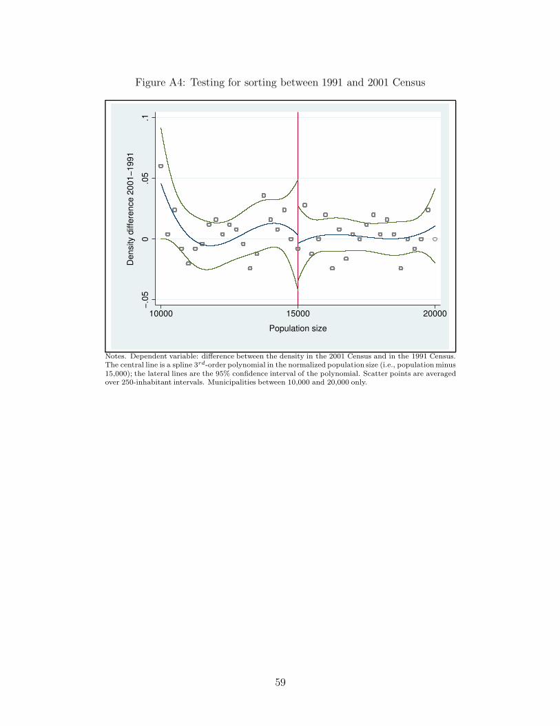
Figure A4: Testing for sorting between 1991 and 2001 Census

−.0

50

.05

.1

De

nsity d

iffe

ren

ce

20

01

−1

99

1

10000 15000 20000

Population size

Notes. Dependent variable: difference between the density in the 2001 Census and in the 1991 Census.The central line is a spline 3rd-order polynomial in the normalized population size (i.e., population minus15,000); the lateral lines are the 95% confidence interval of the polynomial. Scatter points are averagedover 250-inhabitant intervals. Municipalities between 10,000 and 20,000 only.

59

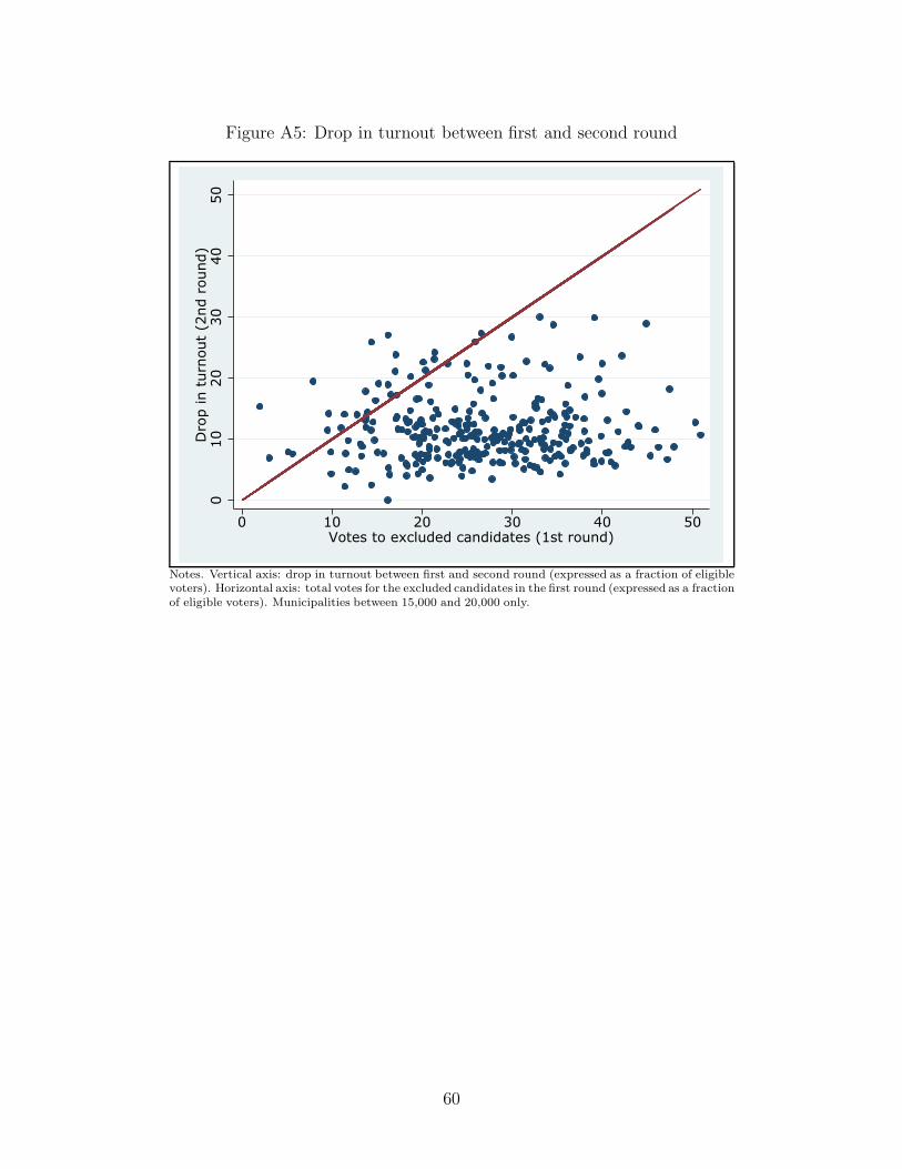
Figure A5: Drop in turnout between first and second round

010

20

30

40

50

Dro

p in t

urn

out

(2nd r

ound)

0 10 20 30 40 50Votes to excluded candidates (1st round)

Notes. Vertical axis: drop in turnout between first and second round (expressed as a fraction of eligiblevoters). Horizontal axis: total votes for the excluded candidates in the first round (expressed as a fractionof eligible voters). Municipalities between 15,000 and 20,000 only.

60

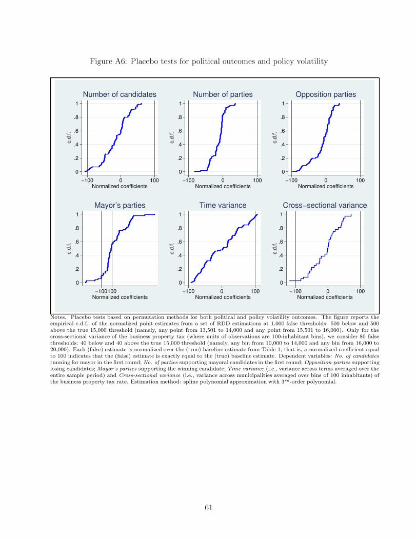
Figure A6: Placebo tests for political outcomes and policy volatility

0

.2

.4

.6

.8

1

c.d

.f.

−100 0 100Normalized coefficients

Number of candidates

0

.2

.4

.6

.8

1

c.d

.f.

−100 0 100Normalized coefficients

Number of parties

0

.2

.4

.6

.8

1

c.d

.f.

−100 0 100Normalized coefficients

Opposition parties

0

.2

.4

.6

.8

1

c.d

.f.

−100100Normalized coefficients

Mayor’s parties

0

.2

.4

.6

.8

1

c.d

.f.

−100 0 100Normalized coefficients

Time variance

0

.2

.4

.6

.8

1

c.d

.f.

−100 0 100Normalized coefficients

Cross−sectional variance

Notes. Placebo tests based on permutation methods for both political and policy volatility outcomes. The figure reports theempirical c.d.f. of the normalized point estimates from a set of RDD estimations at 1,000 false thresholds: 500 below and 500above the true 15,000 threshold (namely, any point from 13,501 to 14,000 and any point from 15,501 to 16,000). Only for thecross-sectional variance of the business property tax (where units of observations are 100-inhabitant bins), we consider 80 falsethresholds: 40 below and 40 above the true 15,000 threshold (namely, any bin from 10,000 to 14,000 and any bin from 16,000 to20,000). Each (false) estimate is normalized over the (true) baseline estimate from Table 1; that is, a normalized coefficient equalto 100 indicates that the (false) estimate is exactly equal to the (true) baseline estimate. Dependent variables: No. of candidates

running for mayor in the first round; No. of parties supporting mayoral candidates in the first round; Opposition parties supportinglosing candidates; Mayor’s parties supporting the winning candidate; Time variance (i.e., variance across terms averaged over theentire sample period) and Cross-sectional variance (i.e., variance across municipalities averaged over bins of 100 inhabitants) ofthe business property tax rate. Estimation method: spline polynomial approximation with 3rd-order polynomial.

61