MODERN FERRITE TECHNOLOGY

SECOND EDITION

MODERN FERRITE TECHNOLOGY

SECOND EDITION

Alex Goldman Pittsburgh, PA, USA

^ Springer

Alex Goldman Ferrite Technology Pittsburgh, PA, USA

Modem Ferrite Technology, 2"" Ed

Library of Congress Control Number: 2005933499

ISBN 10: 0-387-28151-7 ISBN 13: 978-0-387-28151-3 ISBN 10: 0-387-29413-9 (e-book)

Printed on acid-free paper.

© 2006 Springer Science+Business Media, Inc. All rights reserved. This work may not be translated or copied in whole or in part without the written permission of the publisher (Springer Science+Business Media, Inc., 233 Spring Street, New York, NY 10013, USA), except for brief excerpts in connection with reviews or scholarly analysis. Use in connection with any form of information storage and retrieval, electronic adaptation, computer software, or by similar or dissimilar methodology now known or hereafter developed is forbidden. The use in this publication of trade names, trademarks, service marks and similar terms, even if they are not identified as such, is not to be taken as an expression of opinion as to whether or not they are subject to proprietary rights.

Printed in the United States of America.

9 8 7 6 5 4 3 2 1 SPIN 1139477

springeronline. com

Dedication

This book is dedicated to the memory of Professor Takeshi Takei. Professor Takei, to whom I dedicated the first edition of this book and whose preface to that book follows this dedication, was a greatly loved friend and teacher of mine. He passed away on March 12, 1992. He will be remembered as a founding father of ferrites, a great teacher and the organizer of ICF (International Conference on Ferrites). Prof. Takei can truly be regarded as the "father of Modern Ferrites". In addition to his pioneering efforts in the early 1930's, he was a guiding light as a teacher of young scientists and engineers and an inspiration to use one's imagination and work hard. He is sorely missed by the whole ferrite community

Table of Contents

Forward by Takeshi Takei xi

Preface xi

Preface to Second Edition xiii

Acknowledgements xv

Chapter 1: Basics of Magnetism—Source of Magnetic Effect 1

Introduction 1 Magnetic Fields 1 The Concept of Magnetic Poles 2 Electromagnetism 5 Atomic Magnetism 5 Paramagnetism and Diamagnetism 9 Ferromagnestism 10 Antiferromagnetism 11 Ferrimagnetism 13 Paramagnetism above the Curie Point 14 Summary 14

Chapter 2: The Magnestization in Domains and Bulk Materials 17

Introduction 17 The Nature of Domains 17 Proof of the Existence of Domains 21 The Dynamic Behavior of Domains 23 Bulk Material Magnetization 24 MKSA Units 28 Hysteresis Loops 28 Permeability 30 Magnetocrystalline Anisotropy Constants 31 Magnetostriction 32 Important Properties for Hard Magnetic Materials 33 Summary 34

Chapter 3: AC Properties of Ferrites 35

Introduction 35 AC Hysteresis Loops 35 Eddy Current Losses 35 Permeability 38 Disaccomamodation 42 Core Loss 43 Microwave Properties 44 Microwave Precessional Modes 47 Logic and Switching Properties of Ferrites 48

viii MODERN FERRITE TECHNOLOGY

Properties of Recording Media 49 Summary 49

Chapter 4: Crystal Structure of Ferrites 51

Introduction 51 Classes of Crystal Structures in Ferrites 51 Hexagonal Ferrites 63 Magnetic Rare Earth Garnets 65

Chapter 5: Chemical Aspects of Ferrites 71

Intrinsic and Extrinsic Properties of Ferrites 71 Magnetic Properties Under Consideration 71 Mixed Ferrites for Property Optimization 72 Temperature Dependence of Initial Permeability 89 Time Dependence—Initial Permeability (Disaccomodation) 92 Chemistry Dependence—Low Field Losses (Loss Factor) 93 Chemistry Considerations for Hard Ferrites 104 Saturation Induction—^Microwave Ferrites and Garnets 104 Ferrites for Memory and Recording Applications 106

Chapter 6: Microstructural Aspects of Ferrites I l l

Introduction I l l Summary 146

Chapter 7: Ferrite Processing 151

Introduction 151 Powder Preparation—Raw Materials Selection 151 Nonconventional Processing 163 Nanocrystalline Ferrites 166 Powder Preparation of Microwave Ferrites 174 Hard Ferrite Powder Preparation 175

Chapter 8: Applications and Functions of Ferrites 217

Introduction 217 History of Ferrite Applications 217 General Categories of Ferrite Applications 218 Ferrites at D.C. Applications 219 Power Applications 219 Entertainment Applications 221 High Frequency Power Supplies 223 Microwave Applications 224 Magnetic Recording Applications 224 Miscellaneous Applications 226 Summary 226

Chapter 9: Ferrites for Permanent Magnetic Applications 227

Introduction 227 History of Permanent Magnets 227 General Properties of Permanent Magnets 228

TABLE OF CONTENTS ix

Types of Hard Ferrites Materials 232 Criteria for Choosing a Permanent Magnet Material 232 Stabilization of Permanent Magnets 237 Cost Considerations in Permanent Magnet Materials 237 Cost of Finished Magnets 238 Optimum Shapes of Ferrite and Metal Magnets 238 Recoil Lines—Operating Load Lines 238 Commercial Oriented and Non—Oriented Hard Ferrites 238 Summary 242

Chapter 10: Ferrite Inductors and Transformers for Low Power Applications243

Introduction 243 Inductance 244 Effective Matnetic Parameters 245 Measurements of Effective Permeability 247 Magnetic Considerations: Low-Level Applications 248 Flux Density Limitations in Ferrite Inductor Design 260 Surface—Mount Design for Pot Cores 262 Low Level Transformers 262 Ferrites for Low—Level Digital Applications 266 ISDN Components and Materials 268 Low Profile Ferritecores for Telecommunications 269 Multi-Layer Chip Inductors and LC Filters 270

Chapter 11: Ferrites for EMI Suppression 273

Introduction 273 The Need for EMI Suppression Devices 273 Materials for EMI Suppression 275 Frequency Characteristics of EMI Materials 278 The Mechanism of EMI Suppression 279 Components for EMI Suppression 281 Differential Mode Filters 286

Chapter 12: Ferrites For Entertainment Applications—Radio and TV 291

Introduction 291 Ferrite TV Picture Tube Deflection Yokes 291 Materials for Deflection Yokes 293 Flyback Transformers 297 General Purpose Cores for Radio and Television 299 Ferrite Antennas for Radios 300 Summary 306

Chapter 13: Ferrite Transformers and Inductors at High Power 307

Introduction 307 The Early Power Applications of Ferrites 307 Power Transformers 308 Frequency—Voltage Considerations 308 Frequency—Loss Considerations 309 The Hysteresis Loop for Power Materials 310

X MODERN FERRITE TECHNOLOGY

Inverters and Converters 312 Choosing the Right Component for a Power Transformer 313 Choosing the BestFerrite Material 314 Permeability Considerations 318 Output Power Considerations 319 Power Ferrites VS Competing Magnetic Materials 320 Power Ferrite Core Structures 320 Planar Technology 330 High Frequency Applications 324 Determining the Size of the Core 324 Aids in Power Ferrite Core Design 324 Competitive Power Materials for High Frequency 346 Ferroresonant Transformers 347 Power Inductors 348

Chapter 14: Ferrites for Magnetic Recording 353

Introduction 353 Other Digital Magnetic Recording Systems 358 Magnetic Recording Media 361 Magnetic Recording Heads 362 Magnetoresistive Heads 362

Chapter 15: Ferrites for Microwave Applications 375

Introduction 375 The Need for Ferrite Microwave Components 375 Ferrite Microwave Components 376 Commercially Available Microwave Materials 384 Summary 384

Chapter 16: Miscellaneous Ferrite Applications 387

Introduction 387 Summary 393

Chapter 17: Physical, Mechanical and Thermal Aspects of Ferrites 395

Introduction 396 Summary 401

Chapter 18: Magnetic Measurements on Ferrite Materials and Components.403

Introduction 403 Measurements of Magnetic Field Strength 403

Appendix 1 427

Appendix! 433

Index 435

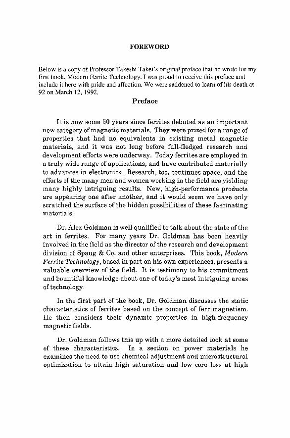
FOREWORD

Below is a copy of Professor Takeshi Takei's original preface that he wrote for my first book, Modern Ferrite Technology. I was proud to receive this preface and include it here with pride and affection. We were saddened to learn of his death at 92 on March 12, 1992.

Preface

It is now some 50 years since ferrites debuted as an important new category of magnetic materials. They were prized for a range of properties that had no equivalents in existing metal magnetic materials, and it was not long before full-fledged research and development efforts were underway. Today ferrites are employed in a truly wide range of applications, and have contributed materially to advances in electronics. Research, too, continues apace, and the efforts of the many men and women working in the field are yielding many highly intriguing results. New, high-performance products are appearing one after another, and it would seem we have only scratched the surface of the hidden possibilities of these fascinating materials.

Dr. Alex Goldman is well qualified to talk about the state of the art in ferrites. For many years Dr. Goldman has been heavily involved in the field as the director of the research and development division of Spang & Co. and other enterprises. This book, Modern Ferrite Technology, based in part on his own experiences, presents a valuable overview of the field. It is testimony to his commitment and bountiful knowledge about one of today^s most intriguing areas of technology.

In the first par t of the book, Dr. Goldman discusses the static characteristics of ferrites based on the concept of ferrimagnetism. He then considers their dynamic properties in high-frequency magnetic fields.

Dr. Goldman follows this up with a more detailed look at some of these characteristics. In a section on power materials he examines the need to use chemical adjustment and microstructural optimization to at tain high saturation and low core loss at high

xii MODERN FERRITE TECHNOLOGY

frequencies. He uses anisotropy and fme particle concepts to describe permanent magnetic ferrites, and reviews how gyromagnetic properties help explain the actions of microwave ferrites.

In a section on applications, he introduces such production technologies-some conventional, some unconventional-as coprecipitation, spray roasting and single crystal preparation. He also discusses some of the special difficulties that ferrites can pose from a design point of view in actual applications. Turning to the subject of magnetic recordings, Dr. Goldman discusses in detail the impressive strides being made in magnetic media and magnetic head applications.

The book is rounded out with valuable appendices, including listings of the latest physical, chemical and magnetic data available on ferrites and listings of world ferrite suppliers.

Modern Ferrite Technology presents the reader with the latest thinking on ferrites by the scientists, researchers and technicians actually involved in their development, leavened with the rich experiences over many years of the author himself. It is a work of great interest not only to those researching new ferrite materials and applications, but to all in science and industry who use ferrites in their work.

April 1987

Takeshi Takei

Preface to Second Edition A number of years have passed since the first edition of Modern Ferrite Technology was published. Four ICF's (International Conference on Ferrites) have taken place since then ie.l992 (Kyoto), 1996 (Bordeaux), 2000 (Kyoto) and 2004 (San Francisco). During that time, so many significant events have occurred in the field of ferrites that the author was prompted to undertake an updating and expansion of the material in the first edition. In the area of new materials, ferrites with permeabilities of 20,000 and 30,000 have been made available commercially , albeit only in small toroids, but still an impressive accomplishment. In addition, power ferrites which have expanded greatly during this time have now been available for frequencies up to 3 MHz. in MnZn ferrites and to 10 MHz. for NZn ferrites. In the field of ceramic processing, the whole area of nanostructured ferrites has come roaring in and while commercial utilization of these materials have not full been exploited to date, the scientific work has been outstanding. In the area of ownership and geographical changes in location of commercial ferrite manufacturers, the scene has changed dramatically. Companies such as Siemens, Philips and Thomson CSF. Have had ownership changes. The geographical center for large scale ferrite production has changed from Japan where it was 30 years ago to China which, it is estimated to have about 60-70% of the world's ferrite proction in the late 2000's. In addition to these new factors, the author has also inserted several new chapters on ferrite applications not covered in the first edition. They are;

1. Ferrites for EMI Suppression Applications 2. Ferrites for Entertainment Applications 3. Ferrites for Magnetic Recording 4. Ferrites for Microwave Applications 5. Ferrite Functions and Applications

The new edition of the book is divided into two parts, the first describing the properties and processing of ferrites and the second part on the functions and applications of ferrites. The chapters on chemistry, microstructure have been expanded to accommodate the new findings. The section on component design have been minimized but section on design aids such as networking have been included.

In the first edition of Modern Ferrite Technology, I remarked that ferrites were "the new kids on the block". Well, by now, the kids have turned into teenagers and, as such, are making their presence felt. In expanding my earlier book. Modern Ferrite Technology, I am attempting to accomplish several objectives;

1. To update the information on ferrites to include the advances since the original work including the major features of ICF6 and ICF7, ICF8 and ICF9

2. To provide a method of comparison of the main features of all the commercially available ferromagnetic materials (and some that are not available such as the Colossal Magnetoresistive Materials).

xiv MODERN FERRITE TECHNOLOGY

3. To add chapters on magnetic materials of expanding importance, such as those for EMI suppression and for entertainment applications

4. To introduce the magnetic materials and components for new technologies such as ISDN, planar magnetics, surface-mount techniques, magnetoresistive recording and integrated magnetics.

As I wrote in the preface in my first book, the attempt here is to describe in as non-technical language as possible, the material, magnetic, and stability characteristics of a wide variety of ferrite materials. The book is aimed at several different audiences. The first chapter takes a broad view of all the applications and functions of magnetic materials. This chapter would appeal to somebody just getting his or her feet wet in the Sea of Magnetism without getting into the materials themselves. The next three chapters are also introductory in nature and deal with the basic concepts of origins of magnetic phenomena, domain and magnetization behavior, magnetic and electrical units and finally to the the action of magnetic materials under ac drive.. We then shift to the ferrite materials and the next three chapters deal with the material properties including crystal structure, chemistry and microstructure. These sections are then followed by a chapter on processing of ferrites. The first part of this book has dealt mainly with the material science aspects of ferromagnetism. Most of the rest of the book is involved with the specific applications. First, we will try to make use of the special properties of the materials we have studied in the low power or telecommunication area, then the associated EMI and entertainment uses. Finally we come to the very large and important chapter on high frequency power materials and components. The next chapter discusses the materials for magnetic recording. The sections on magnetoresistive and magneto-optical recording have been expanded to include the new developments. The next chapter deals with the materials for microwave applications and the last application section is on miscellaneous materials that includes materials for theft deterrence and anechoic chamber tiles. The final chapters discuss the mechanical and thermal aspects ending with a chapter on magnetic measurements. A listing of the lEC documents appear at the end of this chapter. The appendices include abbreviations and symbols, listing of major ferrite suppliers of the world and units conversion from cgs to MKS. As I described in the preface to the earlier book, I would hope that this book also provides a bridge between the material scientist and the electrical design engineer so that some common ground can be established and an understanding of the problems of each can be gained.

Alex Goldman

ACKNOWLEDGEMENTS

ACKNOWLEDGEMENTS I would like to thank Joseph F. Huth III and Harry Savisky of the Magnetics

Div. of Spang and Co. for providing me with some of the photos, photomicrographs and figures in the book. Mr. Richard Parker and Mr. John Knight of Fair-Rite products also provided me with important information on EMI and permanent magnet materials. I would also like to thank the people at Fair-Rite Products, Steward, Arnold Engineering, Magnetics, TDK and FDK for their catalog data. I would like thank Prof.M. Sugimoto for the material from ICF6, ICF7, ICF8 and ICF9. Finally, I would like to thank my wife, Adele, who put up with my endless hours at the computer with great love and understanding and also to my children, Drs. Mark, Beth and Karen for lots of pride and inspiration that they have given to me.

1 BASICS OF MAGNETISM-SOURCE OF MAGNETIC EFFECT

INTRODUCTION This chapter introduces the reader to some of the fundamentals of magnetism and the derivation of magnetic units from a physico-mathematical basis. Next, we apply these units to quantify the intrinsic magnetic properties of electrons, atoms and ions. In later chapters, we extend these properties to crystals, and finally, to bulk material. These properties are intrinsic, that is, they depend only upon the chemistry and crys­tal structure at a particular temperature. Following this examination of intrinsic properties, we will discuss those which, in addition,, depend upon physical charac­teristics as stress, grain structure and porosity. Finally, we correlate the previously defined units to functional magnetic parameters under dynamic conditions such as those used in electrical devices. At first, the magnetic units are derived primarily from the cgs system that is the more conventional one for basic magnetic properties. When the emphasis is shifted to component and application consideration, both cgs and meter-kilogram-second-ampere (mksa) (SI) units are used.

MAGNETIC FIELDS A magnetic field is a force field similar to gravitational and electrical fields; that is, surrounding a source of potential, there is a contoured sphere of influence or field. In the case of gravitation, the source of potential is a mass. For electrical fields, the source is a positive or negative electrical charge. Fields (magnetic or otherwise) can be detected only by the use of a probe, which is usually another source of that type of potential. The criterion that is used is the measurement of a force, either repul­sive or attractive, that is experienced by the probe under the influence of the field. For gravitation, where the interaction is always attractive, the governing equation is:

F = G X mass(l) x mass(2)/ r [1-1] where :F = force (in newtons)

G = constant =6.67 x 10 " nt-m^Kgm^ mass(l)&mass(2) = masses (in kg)

r = distance between masses (in meters)

In the case of an electrical field, the corresponding equation is:

F = Kxqiq2/r^ [1-2] Where: qi, qi = electric charges (Cs)

K = Electrostatic constant = 9x lO^nt-mV(C)^

r = distance between charges (in meters)

2 MODERN FERRITE TECHNOLOGY

The force is repulsive if the two charges are of the same sign and attractive if the signs are different.

Early workers examining magnetic fields found that the origin of the magnetic effect appeared to originate near the ends of the magnets. These sources of magnetic potential are known as magnetic poles. For the magnetic field, there is one main difference compared to the other types of fields. In the gravitational or electrical analogs, the potential producing entities, mass or q, can exist separately. Thus, positive or negative electrical charge can be accumulated separately. In the mag­netic case, the two types of magnetic field-producing species appear to be coupled together as a dipole. Thus far, we have not detected isolated magnetic monopoles.

THE CONCEPT OF MAGNETIC POLES The poles concept was originated a long time ago when the only method of studying magnetic phenomena was based on the interaction of permanent magnets. Although our theories have become much more refined since then, the pole concept is still a useful device in discussions and calculations on ferromagnetism. Poles are ficti­tious points near the end of a magnet where one might consider all the magnetic forces on the magnet to be concentrated. The strength of a pole is determined by the force exerted on it by another pole. In 1750, John Mitchell measured the forces between magnets and found, for example that the attraction or repulsion decreased in proportion to the squares of the distances between the poles of two magnets. Similar to the gravitational and electrical examples, the force is given by:

F = K'mim2/r^ [1-3] Where; mi m2 = strengths of the two poles

K' = a constant which has the value of: = 1 in the cgs system = l/4|io in the MKSA system

where|io=4 xlO'^ henries/m |io=permeability of vacuum

A unit pole (in the cgs system) is defined as one that exerts a force of 1 dyne on a similar unit pole 1 cm away. The force is repulsive if the poles are alike or attrac­tive if they are unlike. Around each pole is a region where it can exert a force on another pole. We call this region the magnetic field. Each point in a magnetic field is described by a field strength or intensity and a field direction which varies with location with respect to the poles. A visualization of the field directions can be made if iron filings are sprinkled on a sheet of paper covering a magnet. The lines indicate the changing directions of the field emanating from the poles. The direction is also that to which a North-seeking end of a compass needle placed at that spot would point. The field strength can be visualized by the density of the lines in any one particular area. The density should fall off according to the inverse square of the distance from the poles as predicted.

The polarity of the magnet itself must be defined, the assignment being such that the North-seeking pole is the North pole of the magnet. Since opposite poles attract, the north- seeking pole of the magnet is actually the same kind of pole as the South pole of the planet. In other words, the north magnetic pole of the planet is the

BASICS OF MAGNETISM -SOURCE OF MAGNETIC EFFECT 3

opposite kind of pole from the North pole of all other physical objects with mag­netic properties. The absolute direction of a magnetic field outside of a magnet is from the north pole to the south pole. Since lines of magnetic field must be con­tinuous, the direction of the field inside the magnet is from south to north poles. The unit of magnetic field intensity called an oersted is defined as that exerted by a field located 1 cm. from a unit pole. The magnetic field intensity can also be defined in terms of current flowing through a wire loop. In the MKSA system of units, the unit of field strength is the ampere- turn per meter, which then relates the magnetic field to this current flow.

mH

>-//

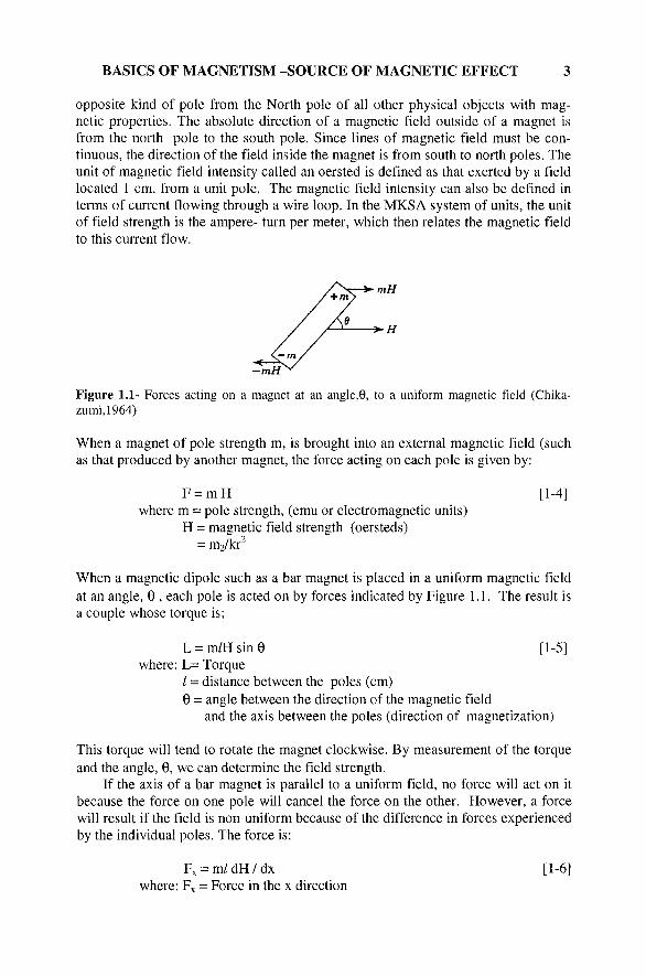
Figure 1.1- Forces acting on a magnet at an angle,9, to a uniform magnetic field (Chika-zumi,1964)

When a magnet of pole strength m, is brought into an external magnetic field (such as that produced by another magnet, the force acting on each pole is given by:

F = mH [1-4] where m = pole strength, (emu or electromagnetic units)

H = magnetic field strength (oersteds) = m2/kr

When a magnetic dipole such as a bar magnet is placed in a uniform magnetic field at an angle, 9 , each pole is acted on by forces indicated by Figure 1.1. The result is a couple whose torque is;

L = m/Hsin0 [1-5] where: L= Torque

/ = distance between the poles (cm) 0 = angle between the direction of the magnetic field

and the axis between the poles (direction of magnetization)

This torque will tend to rotate the magnet clockwise. By measurement of the torque and the angle, 0, we can determine the field strength.

If the axis of a bar magnet is parallel to a uniform field, no force will act on it because the force on one pole will cancel the force on the other. However, a force will result if the field is non-uniform because of the difference in forces experienced by the individual poles. The force is:

F, = m/dH/dx [1-6] where: Fv = Force in the x direction

4 MODERN FERRITE TECHNOLOGY

dH/dx = Change in the magnetic field per centimeter in the X direction

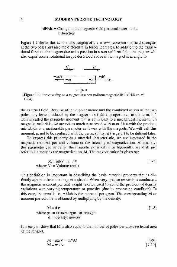
Figure 1,2 shows this action. The lengths of the arrows represent the field strengths at the two poles and also the difference in forces it creates. In addition to the transla-tional force on the magnet due to its position in a non-uniform field, the magnet will also experience a rotational torque described above if the magnet is at angle to

- ^ —i -mH

+ m mH

>-

Figure 1.2- Forces acting on a magnet in a non-uniform magnetic field (Chikazumi, 1964)

the external field. Because of the dipolar nature and the combined action of the two poles, any force produced by the magnet in a field is proportional to the term, ml. This is called the magnetic moment that is equivalent to a mechanical moment. In magnetic materials, we are not as much concerned with m or / but with the product, m/, which is a measurable parameter as it was with the magnets. We will call this moment, |a, not to be confused with the permeability, |i (large | i ) to be defined later.

To express this property as a material characteristic, we are interested in the magnetic moment per unit volume or the intensity of magnetization. Alternately, this parameter can be called the magnetic polarization or frequently, we shall just refer to it simply as the magnetization, M. The magnetization is given by;

M = m//V = | i / V [1-7] where: V = Volume (cm^)

This definition is important in describing the basic material property that is dis­tinctly separate from the magnetic circuit. When very precise research is conducted, the magnetic moment per unit weight is often used to avoid the problem of density variations with varying temperature or porosity (due to processing condition). In this case, the term is a, which is the moment per gram. The corresponding M or moment per volume is obtained by multiplying by the density.

M = d a [1-8] where ;a = moment /gm or emu/gm

d = density, gm/cm"

It is easy to show that M is also equal to the number of poles per cross sectional area of the magnet.

M = m/A^ = m//A/ [1-9] M = m/A [1-10]

BASICS OF MAGNETISM -SOURCE OF MAGNETIC EFFECT 5

where ;A = Cross sectional area (cm^)

As we shall see later, M can be measured relative to a material (powder, chunk, etc.) or in some cases, electrically relative to a magnetic core. The importance of this alternate definition will become more evident in later chapters when the magnetic circuit is discussed in terms of magnetic flux density of which M is a contributing (often a major ) factor.

The magnetization, M, (sometimes called the magnetic polarization) has cgs units called emu/cm^ or often just electro-magnetic units (emu). The MKSA unit for the magnetization is the Tesla or weber/ m . There are 796 emu/cm^ per Tesla or weber/m^.

ELECTROMAGNETISM The real beginning of modern magnetism as we know it today began in 1819 when Hans Oersted discovered that a compass needle was deflected perpendicular to a current bearing wire when the two were placed close to one another. It was at this point that electromagnetism was born. Next, Michael Faraday (1791-1867) discov­ered the opposite effect, namely that an electric voltage can be produced when a conducting wire cut a magnetic field.

ATOMIC MAGNETISM The work on electromagnetism in the early 1800's clarified the relationship between magnetic forces and electric currents in wires, but did little to explain magnetism in matter, which was the older problem. The theories of that time had assumed that one or more fluids were present in magnetic substances with some separation oc­curred at the poles when the material was magnetized. In 1845, Faraday discovered that all substances were magnetic to some degree. Paramagnetic substances were weakly attracted , diamagnetic substances were weakly repelled and ferromagnetics were strongly attracted. The French physicist, P. Curie (1895), today best known for his work on of radioactivity, measured the paramagnetism and diamagnetism in a great number of substances and showed how these properties varied with tempera­ture.

Nineteenth-century scientists were still looking for the link between electro­magnetism and atomic magnetism. In considering the similarity between magnets and current circuits, Andre Ampere( 1775-1836) suggested the existence of small molecular currents which would, in effect make each atom or molecule an individ­ual permanent magnet. These atomic magnets would be pointed in all directions, but would arrange themselves in a line when they were placed in a magnetic field. The expression "Amperian currents" is still used today. The search for a source of these molecular currents ended with the discovery of the electron at the close of the 19th century and reported by J. J.Thompson (1903). By 1905, There was general agreement that the molecular currents responsible for the magnetism in matter were due to electrons circulating in the molecules or atoms.

Bohr Theory of Magnetism In 1913, Niels Bohr (1885-1962) described the quantum theory of matter to account for many of the effects that physicists of the day could not explain. In this theory, he electrons were said to revolve about the nucleus of an atom in orbits, similar to

6 MODERN FERRITE TECHNOLOGY

those of the planets around the sun. The magnetic behavior of an atom was consid­ered to be the result of the orbital motion of the electrons, an effect similar to a cur­rent flowing in a wire loop. The motion of the electrons could be described in fun­damental units so that the magnetic moment accompanying the orbital moment could also be described. The basic unit of electron magnetism is called the Bohr magneton. Not only a fundamental electric charge but also a magnetic quantity is connected with the electron.

As described by classical in Glasstone (1946), the magnetic moment, |i, result­ing from an electron rotating in its orbit can be given by;

\i= ep/2mc [1-11] Where e = electronic charge of the electron (C)

p = total angular momentum of the electron m = mass of the electron, g c = speed of light, cm/s

In the Bohr theory, the orbital angular momentum is quantized in units of h/2n (where h is Planck's constant). Therefore, for the Bohr orbit nearest to the nucleus, the orbital angular momentum, p,can be replaced by h/2n .The resulting magnetic moment can be expressed as:

|l = eh/4Tcmc [1-12]

If we substitute for the known values and constants, we obtain

|IB = 9.27 X 10" ^ erg/Oersted [1-13]

This constant, known as the Bohr magneton is the fundamental unit of magnetic moment in the Bohr theory. It is that the result of the orbital motion of one electron in the lowest orbit.

Orbital and Spin Moments and Magnetism The old Bohr theory was deficient in many aspects and even with the Sommerfeld (1916) variation (the use of elliptical versus circular orbits) could not explain many things. In 1925, Goudsmit and Uhlenbeck (1926) postulated the electron spin .At bout that time, Heisenberg (1926) and Schrodinger( 1929) developed wave mechan­ics which was much more successful in accounting for magnetic phenomena. In quantum mechanics, the new source of magnetism is advanced-that of the spin of the electron on its own axis, similar to that of the earth. Since the electron contains electric charge, the spin leads to movement of this charge or electric current that will produce a magnetic moment. Both theoretically and experimentally, it has been found that the magnetic moment associated with the spin moment is almost identi­cally equal to one Bohr magneton. The original equation for the Bohr magneton is changed slightly to include a term, g, known as the spectroscopic splitting factor This factor denotes a ratio between the mechanical angular momentum to magnetic moment. The value of g for pure spin moment is 2 while that for orbital moment is 1 .However, the lowest orbital quantum number for orbital momentum is 1 (number

BASICS OF MAGNETISM -SOURCE OF MAGNETIC EFFECT 7

of units of h/2n) whereas the quantum number associated with each electron spin is ± 1/2.The new equation is:

|Li= gxexn/2mc (2) [1-14] where; for orbital moment(lowest state) g=l, n=l

for spin moment g=2, n=l/2

We can see why the orbital and spin moment both turn out to be equal to 1|XB. We now have a universal unit of magnetic moment that accommodates both the orbital and spin moments of electrons. The Bohr magneton is that fundamental unit. We have originally defined the magnetic moment in connection with permanent mag­nets. The electron itself may well be called the smallest permanent magnet.

The net amount of magnetic moment of an atom or ion is the vector sum of the individual spin and orbital moments of the electrons in its outer shells. In gases and liquids, the orbital contribution to magnetism can be important, but in many solids, including those containing the magnetically-important transition metal elements, strong electric fields found in a crystalline structure destroy or quench the effect. Most magnetic materials are crystalline and therefore would be affected by this fac­tor. In the great majority of the magnetic materials we will deal with (those involv­ing the 3d electrons of transition metals), we will not be concerned with the orbital momentum except for small deviations of the g factor from 2. However, when we talk about the magnetic properties of the rare earths, we cannot ignore the orbital contribution. In these cases, the affected 4f electrons are not outermost. Conse­quently, they are screened from the electric fields by electrons of outer orbitals. This is not the case for the 3d electrons which are in the outermost shell. For the present, however, we will consider the magnetic behavior of most common magnetic mate­rials to be entirely the result of spin moments.

Atomic and Ionic Moments There are two modes of electron spin. Schematically, we can represent them as either clockwise or counter-clockwise. If the electron is spinning in a horizontal plane and counter-clockwise as viewed from above, the direction of the magnetic moment is directed up. If it is clockwise, the reverse is true. The direction of the moment is comparable to the direction of the magnetization (from S to N poles) of a permanent magnet to which the electron spin is equivalent. It is very common to schematically represent the two types electron spin as arrows pointed up or down and we shall use this representation in our discussion. A counter-clockwise spin in an atom (arrow up) will cancel a clockwise spin (arrow up) and no net magnetic moment will result. It is only the unpaired spins that will give rise to a net magnetic moment.

In quantum mechanics, the atoms or ions are built up of electrons in orbitals similar to the Bohr orbits. These orbitals are also classified according to the shape of the spacial electronic probability density. This can be visualized as the superim­posing of very many photographs of the electron at different times .The shape of the electron cloud that results is the shape of the orbital. For example, for s electrons, this shape is the surface of a sphere. Discrete energy levels are associated with each of these orbitals. As we construct the elements of higher atomic numbers, the higher

8 MODERN FERRITE TECHNOLOGY

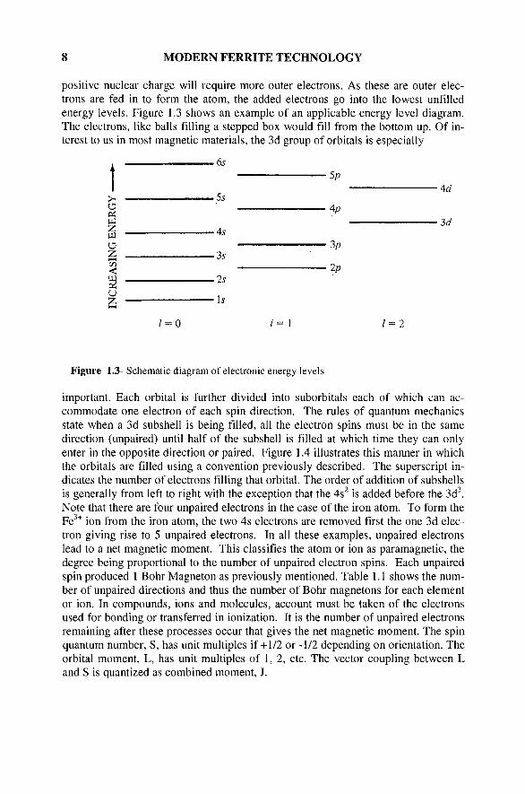
positive nuclear charge will require more outer electrons. As these are outer elec­trons are fed in to form the atom, the added electrons go into the lowest unfilled energy levels. Figure 1.3 shows an example of an applicable energy level diagram. The electrons, like balls filling a stepped box would fill from the bottom up. Of in­terest to us in most magnetic materials, the 3d group of orbitals is especially

.6^ Sp

•4d >H - _ — — _ _ _ 5s O • 4p a 3d § 45 O 3p Z 3s ^ 2p S 2. u . g \s

1=0 / = 1 / = 2

Figure 1.3- Schematic diagram of electronic energy levels

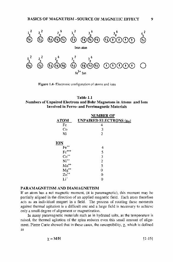
important. Each orbital is further divided into suborbitals each of which can ac­commodate one electron of each spin direction. The rules of quantum mechanics state when a 3d subshell is being filled, all the electron spins must be in the same direction (unpaired) until half of the subshell is filled at which time they can only enter in the opposite direction or paired. Figure 1.4 illustrates this manner in which the orbitals are filled using a convention previously described. The superscript in­dicates the number of electrons filling that orbital. The order of addition of subshells is generally from left to right with the exception that the 4s^ is added before the 3d" . Note that there are four unpaired electrons in the case of the iron atom. To form the Fe " ion from the iron atom, the two 4s electrons are removed first the one 3d elec­tron giving rise to 5 unpaired electrons. In all these examples, unpaired electrons lead to a net magnetic moment. This classifies the atom or ion as paramagnetic, the degree being proportional to the number of unpaired electron spins. Each unpaired spin produced 1 Bohr Magneton as previously mentioned. Table 1.1 shows the num­ber of unpaired directions and thus the number of Bohr magnetons for each element or ion. In compounds, ions and molecules, account must be taken of the electrons used for bonding or transferred in ionization. It is the number of unpaired electrons remaining after these processes occur that gives the net magnetic moment. The spin quantum number, S, has unit multiples if +1/2 or -1/2 depending on orientation. The orbital moment, L, has unit multiples of 1, 2, etc. The vector coupling between L and S is quantized as combined moment, J.

BASICS OF MAGNETISM -SOURCE OF MAGNETIC EFFECT

j 2 2? 2^ 3^ 36 36 42

® ® ®®® ® (R)®® ®®©©© ® Iron atom

J 2 2 „6 32 36

® ® ®(H)® ® ®®® ®©©®® O Fe ^ Ion

Figure 1.4- Electronic configuration of atoms and ions

Table 1.1 Numbers of Unpaired Electrons and Bohr Magnetons in Atoms and Ions

Involved in Ferro- and Ferrimagnetic Materials

ATOM Fe Co Ni

ION Fe^ Fe^^ Co^ Nr Mn^^ Mg^^ Zn^^ Li

NUMBER OF UNPAIRED ELECTRONS (u«)

4 3 2

4 5 3 2 5 0 0 0

PARAMAGNETISM AND DIAMAGNETISM If an atom has a net magnetic moment, (it is paramagnetic), this moment may be partially aligned in the direction of an applied magnetic field. Each atom therefore acts as an individual magnet in a field. The process of rotating these moments against thermal agitation is a difficult one and a large field is necessary to achieve only a small degree of alignment or magnetization.

In many paramagnetic materials such as in hydrated salts, as the temperature is raised, the thermal agitation of the spins reduces even this small amount of align­ment. Pierre Curie showed that in these cases, the susceptibility, %, which is defined as

X = M/H [1-15]

10 MODERN FERRITE TECHNOLOGY

where ;% = susceptibility M = magnetization or moment, emu/cm^ H = Magnetic field strength, Oersteds

follows the Curie Law given as;

X=C/T [1-16] Where: C = Curie constant

T = Temperature in Degrees Kelvin Also; 1/% =T/C [1-17]

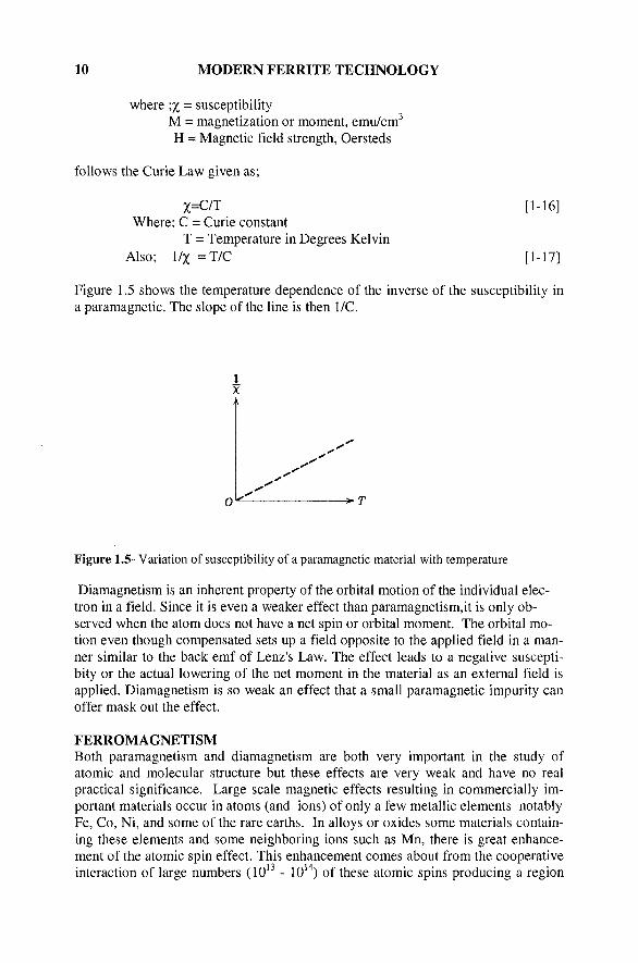
Figure 1.5 shows the temperature dependence of the inverse of the susceptibility in a paramagnetic. The slope of the line is then 1/C.

-^T

Figure 1.5- Variation of susceptibility of a paramagnetic material with temperature

Diamagnetism is an inherent property of the orbital motion of the individual elec­tron in a field. Since it is even a weaker effect than paramagnetism,it is only ob­served when the atom does not have a net spin or orbital moment. The orbital mo­tion even though compensated sets up a field opposite to the applied field in a man­ner similar to the back emf of Lenz's Law. The effect leads to a negative suscepti-bity or the actual lowering of the net moment in the material as an external field is applied. Diamagnetism is so weak an effect that a small paramagnetic impurity can offer mask out the effect.

FERROMAGNETISM Both paramagnetism and diamagnetism are both very important in the study of atomic and molecular structure but these effects are very weak and have no real practical significance. Large scale magnetic effects resulting in commercially im­portant materials occur in atoms (and ions) of only a few metallic elements notably Fe, Co, Ni, and some of the rare earths. In alloys or oxides some materials contain­ing these elements and some neighboring ions such as Mn, there is great enhance­ment of the atomic spin effect. This enhancement comes about from the cooperative interaction of large numbers (10^^ - 10 " ) of these atomic spins producing a region

BASICS OF MAGNETISM -SOURCE OF MAGNETIC EFFECT 11

where all atomic spins within it are aligned parallel (positive exchange interaction). These materials are called ferromagnetic.

The regions of the materials in which the cooperative effect extends are known as magnetic domains. P. Weiss(1907) first proposed the existence of magnetic do­mains to account for certain magnetic phenomena. He postulated the existence of a "molecular field" which produced the interaction aligning spins of neighboring at­oms parallel. W. Heisenberg(1928) attributed this "molecular field" to quan­tum-mechanical exchange forces. Domains have been confirmed by many tech­niques and can be made visible by several means.

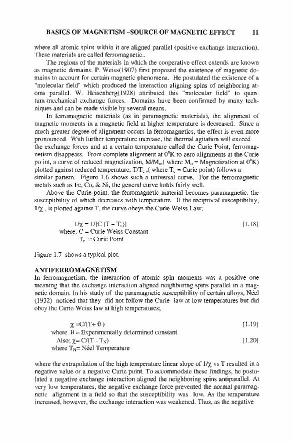
In ferromagnetic materials (as in paramagnetic materials), the alignment of magnetic moments in a magnetic field at higher temperature is decreased. Since a much greater degree of alignment occurs in ferromagnetics, the effect is even more pronounced. With further temperature increase, the thermal agitation will exceed the exchange forces and at a certain temperature called the Curie Point, ferromag-netism disappears. From complete alignment at O K to zero alignments at the Curie po int, a curve of reduced magnetization, M/Mo,( where Mo = Magnetization at 0°K) plotted against reduced temperature, T/Tc,( where Tc = Curie point) follows a similar pattern. Figure 1.6 shows such a universal curve. For the ferromagnetic metals such as Fe, Co, & Ni, the general curve holds fairly well.

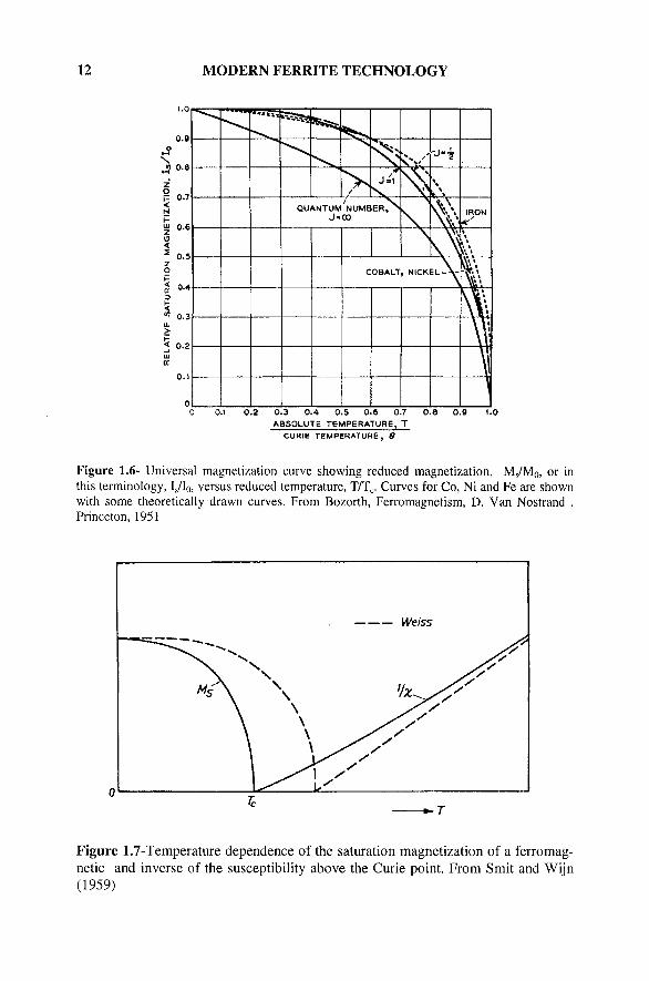
Above the Curie point, the ferromagnetic material becomes paramagnetic, the susceptibility of which decreases with temperature. If the reciprocal susceptibility, 1/% , is plotted against T, the curve obeys the Curie Weiss Law;

1/%=1/[C(T-Te)] [1.18] where: C = Curie Weiss Constant

Tc = Curie Point

Figure 1.7 shows a typical plot.

ANTIFERROMAGNETISM In ferromagnetism, the interaction of atomic spin moments was a positive one meaning that the exchange interaction aligned neighboring spins parallel in a mag­netic domain. In his study of the paramagnetic susceptibility of certain alloys, Neel (1932) noticed that they did not follow the Curie law at low temperatures but did obey the Curie-Weiss law at high temperatures;

X=C/(T+0) [1.19] where 0 = Experimentally determined constant

A 1 S O ; X = C / ( T - T N ) [1.20] where TN= Neel Temperature

where the extrapolation of the high temperature linear slope of 1/% vs T resulted in a negative value or a negative Curie point. To accommodate these findings, he postu­lated a negative exchange interaction aligned the neighboring spins antiparallel. At very low temperatures, the negative exchange force prevented the normal paramag­netic alignment in a field so that the susceptibility was low. As the temperature increased, however, the exchange interaction was weakened. Thus, as the negative

12 MODERN FERRITE TECHNOLOGY

1.0

0.0

N

u 0.6 O < ^ 0.5 z o

5 04 D

^ 0.3 UJ

> < 0.2 UJ oc

O.t

0

1 • ' • • •w wr?5f= ^ ^

/

^ < v -j.'r

QUANTUM'NUMBER,> J«00

- j - i

% W \ IRON

\ 1 . COBALT, N ICKEL-V

L Y » % 1

V vi *

\ 13

).1 0.2 0.3 0.4 0.5 0.6 0.7 0.8 0.9 ABSOLUTE TEMPERATURE,T

CURIE TEMPERATURE, 0

Figure 1.6- Universal magnetization curve showing reduced magnetization, M /Mo, or in this terminology, IJIQ, versus reduced temperature, T/Tc. Curves for Co, Ni and Fe are shown with some theoretically drawn curves. From Bozorth, Ferromagnetism, D. Van Nostrand , Princeton, 1951

*-r

Figure 1.7-Temperature dependence of the saturation magnetization of a ferromag­netic and inverse of the susceptibility above the Curie point. From Smit and Wijn (1959)

BASICS OF MAGNETISM -SOURCE OF MAGNETIC EFFECT 13

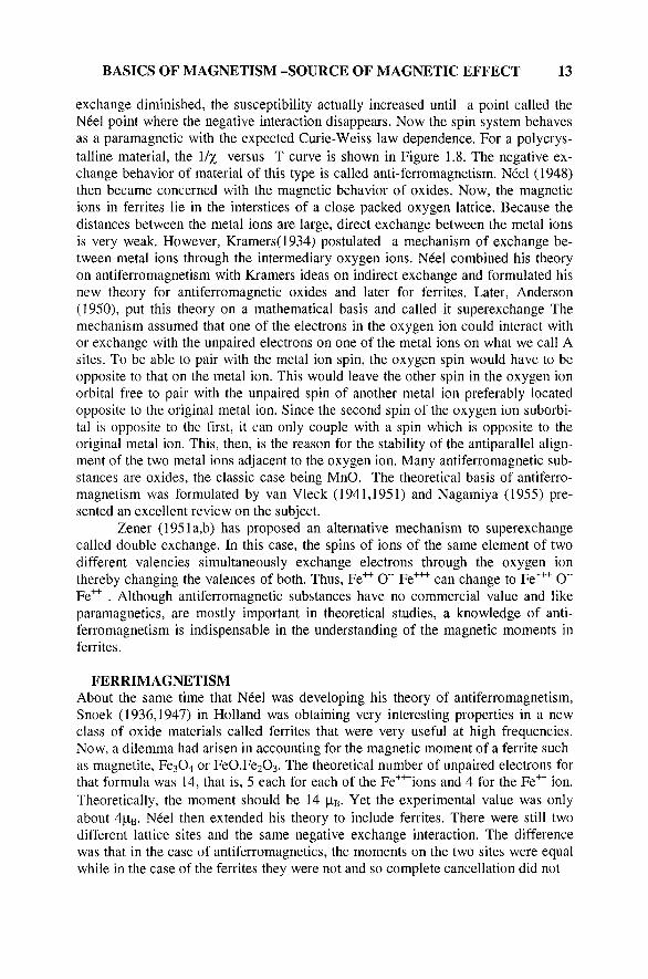
exchange diminished, the susceptibility actually increased until a point called the Neel point where the negative interaction disappears. Now the spin system behaves as a paramagnetic with the expected Curie-Weiss law dependence. For a polycrys-talline material, the 1/% versus T curve is shown in Figure 1.8. The negative ex­change behavior of material of this type is called anti-ferromagnetism. Neel (1948) then became concerned with the magnetic behavior of oxides. Now, the magnetic ions in ferrites lie in the interstices of a close packed oxygen lattice. Because the distances between the metal ions are large, direct exchange between the metal ions is very weak. However, Kramers(1934) postulated a mechanism of exchange be­tween metal ions through the intermediary oxygen ions. Neel combined his theory on antiferromagnetism with Kramers ideas on indirect exchange and formulated his new theory for antiferromagnetic oxides and later for ferrites. Later, Anderson (1950), put this theory on a mathematical basis and called it superexchange The mechanism assumed that one of the electrons in the oxygen ion could interact with or exchange with the unpaired electrons on one of the metal ions on what we call A sites. To be able to pair with the metal ion spin, the oxygen spin would have to be opposite to that on the metal ion. This would leave the other spin in the oxygen ion orbital free to pair with the unpaired spin of another metal ion preferably located opposite to the original metal ion. Since the second spin of the oxygen ion suborbi­tal is opposite to the first, it can only couple with a spin which is opposite to the original metal ion. This, then, is the reason for the stability of the antiparallel align­ment of the two metal ions adjacent to the oxygen ion. Many antiferromagnetic sub­stances are oxides, the classic case being MnO. The theoretical basis of antiferro­magnetism was formulated by van Vleck (1941,1951) and Nagamiya (1955) pre­sented an excellent review on the subject.

Zener (1951a,b) has proposed an alternative mechanism to superexchange called double exchange. In this case, the spins of ions of the same element of two different valencies simultaneously exchange electrons through the oxygen ion thereby changing the valences of both. Thus, Fe"*" O" Fe"*"*" can change to Fe"""*" O" Fe" " . Although antiferromagnetic substances have no commercial value and like paramagnetics, are mostly important in theoretical studies, a knowledge of anti­ferromagnetism is indispensable in the understanding of the magnetic moments in ferrites.

FERRIMAGNETISM About the same time that Neel was developing his theory of antiferromagnetism, Snoek (1936,1947) in Holland was obtaining very interesting properties in a new class of oxide materials called ferrites that were very useful at high frequencies. Now, a dilemma had arisen in accounting for the magnetic moment of a ferrite such as magnetite, Fe304 or FeO.FeiOs. The theoretical number of unpaired electrons for that formula was 14, that is, 5 each for each of the Fe' " "*"ions and 4 for the Fe" " ion. Theoretically, the moment should be 14 |IB- Yet the experimental value was only about 4|LIB' Neel then extended his theory to include ferrites. There were still two different lattice sites and the same negative exchange interaction. The difference was that in the case of antiferromagnetics, the moments on the two sites were equal while in the case of the ferrites they were not and so complete cancellation did not

14 MODERN FERRITE TECHNOLOGY

Figure 1.8-Reciprocal of the susceptibility of an antiferromagnetic material showing the discontinuity at the Neel temperature and the extrapolation of the linear portion to the "nega­tive Curie temperature. From Chikazumi (1959)

occur and a net moment resulted which was the difference in the moments on the two sites. This difference is usually brought about by the difference in the number of magnetic ions on the two types of sites. This phenomenon is called ferrimagnet-ism or uncompensated antiferromagnetism. Neel(1948) published his theory in a paper called Magnetic Properties of Ferrites; Ferrimagnetism and Antiferromagnet­ism. In the preceding year, Snoek(1936) in a book entitled New Developments in Ferromagnetic Materials, disclosed the experimental magnetic properties of a large number of useful ferrites.

The interactions of the net moments of the lattice are continuous throughout the rest of the crystal so that ferrimagnetism can be treated as a special case of ferro-magnetism and thus domains can form in a similar manner.

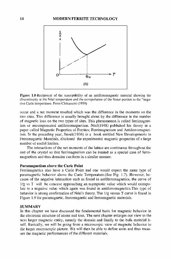
Paramagnetism above the Curie Point Ferrimagnetics also have a Curie Point and one would expect the same type of paramagnetic behavior above the Curie Temperature.(See Fig. 1.7). However, be­cause of the negative interaction such as found in antiferromagnetics, the curve of 1/% vs T will be concave approaching an asymptotic value which would extrapo­late to a negative value which again was found in antiferromagnetics.This type of behavior is strong confirmation of Neel's theory. The 1/% versus T curve is found in Figure 1.9 for paramagnetic, ferromagnetic and ferromagnetic materials.

SUMMARY In this chapter we have discussed the fundamental basis for magnetic behavior in the electronic structure of atoms and ions. The next chapter enlarges our view to the next larger magnetic entity, namely the domain and finally to the bulk material it­self. Basically, we will be going from a microscopic view of magnetic behavior to the larger macroscopic picture. We will then be able to define units and thus meas­ure the magnetic performances of the different materials.

BASICS OF MAGNETISM -SOURCE OF MAGNETIC EFFECT 15

'Ix

t /

y ^

.€^ y y

^y

y y^ 4C

^ N / y^ \ 1

y^ \L.

.s^yy €y / ^

7X ^ / t < ^ > ^

/ !^^

T,

Figure 1.9- Comparison of the temperature tendencies of the reciprocal susceptibilities of paramagnetic, ferromagnetic and ferrimagnetic materials.

References

Anderson,P.W.(1950) Phys. Rev., 79 ,705 Bethe,H. (1933) Handb. d. physik(5) 24 pt.2,595-8 Bohr,N. (1913) Phil. Mag. 5, 476,857 Bozorth,R.B. (1951) Ferromagnetism ,D.Van Nostrand,New York Curie,P. (1895) Ann. chim phys.[7] 5, 289 Glasstone,S. (1946) Textbook of Physical Chemistry,D. Van Nostrand, New York Goudsmit S.(1926) and Uhlenbeck,G.E. Nature, 117,264 Heisenberg,W.(1926) Z. pkysik 38, 411(1928) ibid 49, 619) Kramers,H.A. (1934) Physica, i , 182 Nagamiya,T.(1955) Yoshida,K. and Kubo,R., Adv. Phy, 4, 1-112,Academic P. N.Y Neel,L. (1932) Ann. de Phys. 17, 61(1948) ibid. (12) 3, 137 Snoek,J.L.(1936) Physica (Amsterdam) 3, 463 Snoek,J.L.(1947) New Developments in Ferromagnetic Mat.Elsevier Amsterdam Sommerfeld,A.(1916) Ann. phys. 51, 1 Thompson,J.J.(1903) Phil. Mag. 5, 346 van Vleck, J.H. (1951) J. Phys Rad, 12, 262 Weiss,P. (1907) J. phys.[4] 6,661-90 Zener, C.(1951a) Phys. Rev. 8i, 440 Zener C. (1951b) ibid, 83, 299

2 THE MAGNETIZATION IN DOMAINS AND BULK MATERIALS

INTRODUCTION Thus far, we have discussed the factors that contribute to the atomic and ionic mo­ments and the effect of their magnetic interactions on the moments of the various crystal lattices. These moments are the maximum values or those measured under saturation conditions, at O K., that is, with complete alignment of the net magnetic moments. These values we found were intrinsic properties, that is, they depended only on chemistry and crystal structure (and of course, temperature). We have not discussed the important aspects of domain and bulk material magnetizations. In this chapter, we will expand our scope from the microscopic moment to the larger mo­ment (in domains) and finally to the macroscopic bulk magnetization. Once these are described, we can then turn to the topics of magnetization mechanisms, mag­netization reversal, and ultimately to cyclic magnetization, as in alternating current operation. To obtain a clear picture of these topics, the use of domain theory and domain dynamics is indispensable. This chapter will first discuss these subjects and show how they lead to the bulk magnetic properties.

THE NATURE OF DOMAINS In a ferromagnetic domain, there is parallel alignment of the atomic moments. In a ferrite domain, the net moments of the antiferrimagnetic interactions are spontane­ously oriented parallel to each other (even without an applied magnetic field). The term, spontaneous magnetization or polarization is often used to describe this prop­erty. Each domain becomes a magnet composed of smaller magnets (ferromagnetic moments). Domains contain about 10 ^ to 10 ^ atoms and their dimensions are on the order of microns (lO"" cm.). Their size and geometry are governed by certain considerations. Domains are formed basically to reduce the magnetostatic energy which is the magnetic potential energy contained in the field lines (or flux lines as they are commonly called) connecting north and south poles outside of the material. Figure 2.1 shows the lines of flux in a particle with a single domain. The arrows indicate the direction of the magnetization and consequently the direction of spin alignment in the domain. We can substantially reduce the length of the flux path through the unfavorable air space by spitting that domain into two or more smaller domains. This is shown in Figure 2.2. This splitting process continues to lower the energy of the system until the point that more energy is required to form the domain boundary than is decreased by the magnetostatic energy change. When a large do­main is split into n domains, the energy of the new structure is about l/nih of the single domain structure. In Figure 2.2, the moments in adjacent domains

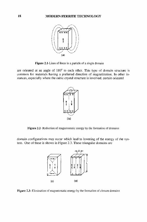
18 MODERN FERRITE TECHNOLOGY

/ /

\ \ I S S S S U / /

I 1 I I I )

(a)

Figure 2,1-Lines of force in a particle of a single domain

are oriented at an angle of 180° to each other. This type of domain structure is common for materials having a preferred direction of magnetization. In other in­stances, especially where the cubic crystal structure is involved, certain oriented

/^ N N

t S S

s s

1 N N

7\

/

(b)

Figure 2.2- Reduction of magnetostatic energy by the formation of domains

domain configurations may occur which lead to lowering of the energy of the sys­tem. One of these is shown in Figure 2.3. These triangular domains are

111

-IT / / / y Y Y Y

ifiliti , A A A

(0 (d)

Figure 2.3- Elimination of magnetostatic energy by the formation of closure domains