Module 0: Introduction to Electronics - MIT OpenCourseWare · 20.309: Biological Instrumentation andMeasurement Laboratory Fall 2006 Module 0: Introduction to Electronics Contents

20.309: Biological Instrumentation andMeasurement Laboratory Fall 2006

Module 0: Introduction to Electronics

Contents

1 Objectives and Learning Goals 1

2 Roadmap and Milestones 2

3 Lab Procedures 23.1 DC measurements . . . . . . . . . . . . . . . . . . . . . . . . . . . . . . . . . . . . . 23.2 Impedance and load . . . . . . . . . . . . . . . . . . . . . . . . . . . . . . . . . . . . 43.3 Photodiode i-v characteristics . . . . . . . . . . . . . . . . . . . . . . . . . . . . . . . 53.4 Time-varying signals and AC measurements . . . . . . . . . . . . . . . . . . . . . . . 63.5 “Black-box” transfer functions . . . . . . . . . . . . . . . . . . . . . . . . . . . . . . 6

A Circuit Components 7A.1 Resistors . . . . . . . . . . . . . . . . . . . . . . . . . . . . . . . . . . . . . . . . . . . 7A.2 Capacitors . . . . . . . . . . . . . . . . . . . . . . . . . . . . . . . . . . . . . . . . . . 8A.3 Diodes . . . . . . . . . . . . . . . . . . . . . . . . . . . . . . . . . . . . . . . . . . . . 8A.4 Breadboards . . . . . . . . . . . . . . . . . . . . . . . . . . . . . . . . . . . . . . . . . 8A.5 Operational Amplifiers . . . . . . . . . . . . . . . . . . . . . . . . . . . . . . . . . . . 10

B Instruments 11B.1 Digital Multimeter (DMM) . . . . . . . . . . . . . . . . . . . . . . . . . . . . . . . . 11B.2 DC Power Supply . . . . . . . . . . . . . . . . . . . . . . . . . . . . . . . . . . . . . . 11B.3 Function Generator . . . . . . . . . . . . . . . . . . . . . . . . . . . . . . . . . . . . . 12B.4 Oscilloscope . . . . . . . . . . . . . . . . . . . . . . . . . . . . . . . . . . . . . . . . . 12B.5 LabVIEW and the data acquisition (DAQ) system . . . . . . . . . . . . . . . . . . . 13

1 Objectives and Learning Goals

1. Familiarize yourself with standard lab electronics and some common circuit elements: linear and nonlinear, passive and active.

2. Understand fundamental electronics concepts, including:

current/voltage dividers •

impedance & load •

frequency response & transfer functions •

3. Analyze and build several circuits, which will be of use later.

This module is an extended lab orientation of sorts. Take this time to explore electronic circuits and really get to know all the features of our lab’s instrumentation. It will pay off later. What you learn and do this week will underpin many of the experiments during the rest of the semester.

Since you are mainly concerned with understanding your toolset and learning its uses and limitations, no formal write-up is necessary. However, many parts of this module work hand-inhand with questions on Problem Set 1, so you will still want to record data for completing them.

1


2 Roadmap and Milestones

1. Practice making DC and AC signal measurements.

2. Measure circuit input and output impedances and observe loading effects.

3. Study the nonlinear characteristics of a diode, and learn how a photodiode responds to incident light.

4. Test several unknown circuits to determine their transfer functions

3 Lab Procedures

3.1 DC measurements

The simplest type of circuit is the direct current (DC) situation. This means simply that the applied voltage does not vary in time. Alternating current (AC) is discussed in Sec. 3.4. Most often, we separate complex signals into their DC and AC components (e.g. a sine wave with a constant offset) to make analysis simpler.

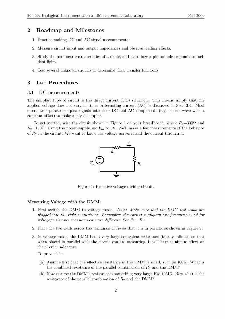
To get started, wire the circuit shown in Figure 1 on your breadboard, where R1=330Ω and R2=150Ω. Using the power supply, set Vin to 5V. We’ll make a few measurements of the behavior of R2 in the circuit. We want to know the voltage across it and the current through it.

Figure 1: Resistive voltage divider circuit.

Measuring Voltage with the DMM:

1. First switch the DMM to voltage mode. Note: Make sure that the DMM test leads are plugged into the right connections. Remember, the correct configurations for current and for voltage/resistance measurements are different. See Sec. B.1

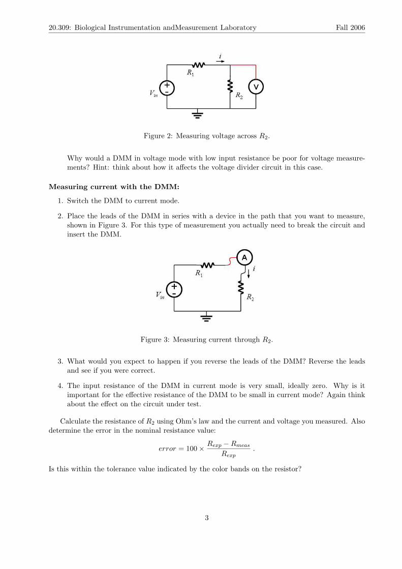
2. Place the two leads across the terminals of R2 so that it is in parallel as shown in Figure 2.

3. In voltage mode, the DMM has a very large equivalent resistance (ideally infinite) so that when placed in parallel with the circuit you are measuring, it will have minimum effect on the circuit under test.

To prove this:

(a) Assume first that the effective resistance of the DMM is small, such as 100Ω. What is the combined resistance of the parallel combination of R2 and the DMM?

(b) Now assume the DMM’s resistance is something very large, like 10MΩ. Now what is the resistance of the parallel combination of R2 and the DMM?

2


Figure 2: Measuring voltage across R2.

Why would a DMM in voltage mode with low input resistance be poor for voltage measurements? Hint: think about how it affects the voltage divider circuit in this case.

Measuring current with the DMM:

1. Switch the DMM to current mode.

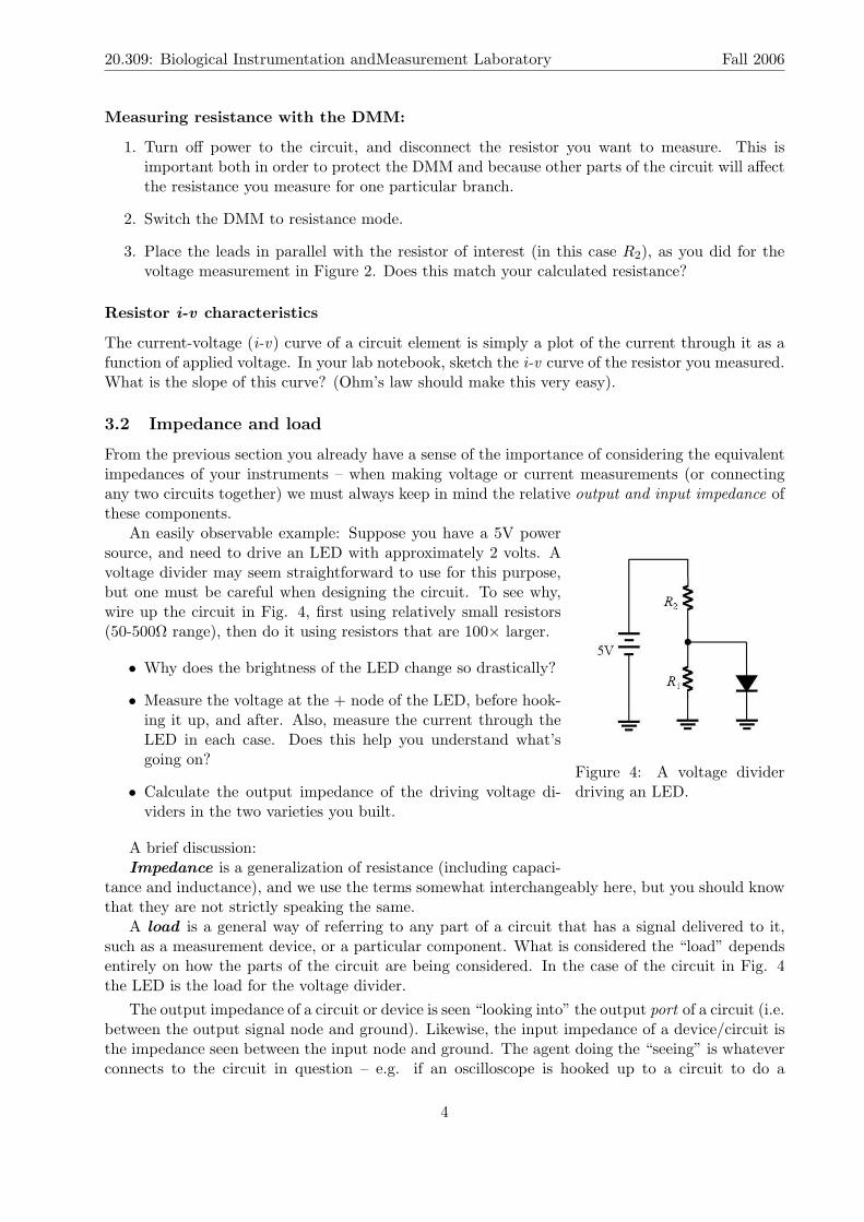
2. Place the leads of the DMM in series with a device in the path that you want to measure, shown in Figure 3. For this type of measurement you actually need to break the circuit and insert the DMM.

Figure 3: Measuring current through R2.

3. What would you expect to happen if you reverse the leads of the DMM? Reverse the leads and see if you were correct.

4. The input resistance of the DMM in current mode is very small, ideally zero. Why is it important for the effective resistance of the DMM to be small in current mode? Again think about the effect on the circuit under test.

Calculate the resistance of R2 using Ohm’s law and the current and voltage you measured. Also determine the error in the nominal resistance value:

error = 100 Rexp − Rmeas

.× Rexp

Is this within the tolerance value indicated by the color bands on the resistor?

3


Measuring resistance with the DMM:

1. Turn off power to the circuit, and disconnect the resistor you want to measure. This is important both in order to protect the DMM and because other parts of the circuit will affect the resistance you measure for one particular branch.

2. Switch the DMM to resistance mode.

3. Place the leads in parallel with the resistor of interest (in this case R2), as you did for the voltage measurement in Figure 2. Does this match your calculated resistance?

Resistor i-v characteristics

The current-voltage (i-v) curve of a circuit element is simply a plot of the current through it as a function of applied voltage. In your lab notebook, sketch the i-v curve of the resistor you measured. What is the slope of this curve? (Ohm’s law should make this very easy).

3.2 Impedance and load

From the previous section you already have a sense of the importance of considering the equivalent impedances of your instruments – when making voltage or current measurements (or connecting any two circuits together) we must always keep in mind the relative output and input impedance of these components.

An easily observable example: Suppose you have a 5V power source, and need to drive an LED with approximately 2 volts. A voltage divider may seem straightforward to use for this purpose, but one must be careful when designing the circuit. To see why, wire up the circuit in Fig. 4, first using relatively small resistors (50-500Ω range), then do it using resistors that are 100× larger.

Why does the brightness of the LED change so drastically? •

Measure the voltage at the + node of the LED, before hook• ing it up, and after. Also, measure the current through the LED in each case. Does this help you understand what’s going on?

Figure 4: A voltage divider Calculate the output impedance of the driving voltage di- driving an LED. • viders in the two varieties you built.

A brief discussion: Impedance is a generalization of resistance (including capaci

tance and inductance), and we use the terms somewhat interchangeably here, but you should know that they are not strictly speaking the same.

A load is a general way of referring to any part of a circuit that has a signal delivered to it, such as a measurement device, or a particular component. What is considered the “load” depends entirely on how the parts of the circuit are being considered. In the case of the circuit in Fig. 4 the LED is the load for the voltage divider.

The output impedance of a circuit or device is seen “looking into” the output port of a circuit (i.e. between the output signal node and ground). Likewise, the input impedance of a device/circuit is the impedance seen between the input node and ground. The agent doing the “seeing” is whatever connects to the circuit in question – e.g. if an oscilloscope is hooked up to a circuit to do a

4


measurement, that circuit “sees” the input impedance of the oscilloscope. Here, the voltage divider being used to drive the LED “sees” the LED’s input impedance, and the LED “sees” the output impedance of the driving circuit.

3.3 Photodiode i-v characteristics

In this section, our aim is to measure and plot the current-voltage relationship for a diode in the transition region from non-conducting to conducting. After that, we also want to measure the behavior of photodiodes (see Sec. A.3, which we’ll use a number of times in the course as light detectors.

Start by covering the window of an FDS100 photodiode with black tape — with no light coming in, it is just a regular diode. Then we’ll illuminate it to see its photodiode action.

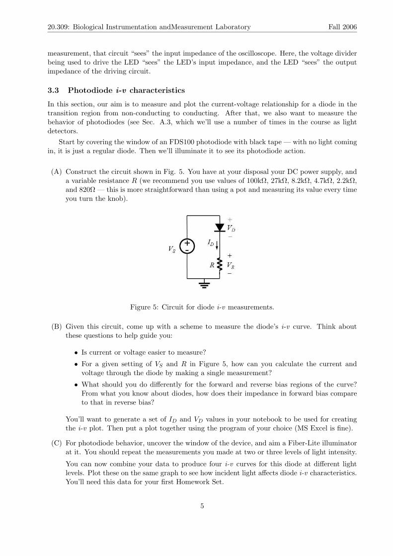
(A) Construct the circuit shown in Fig. 5. You have at your disposal your DC power supply, and a variable resistance R (we recommend you use values of 100kΩ, 27kΩ, 8.2kΩ, 4.7kΩ, 2.2kΩ, and 820Ω — this is more straightforward than using a pot and measuring its value every time you turn the knob).

Figure 5: Circuit for diode i-v measurements.

(B) Given this circuit, come up with a scheme to measure the diode’s i-v curve. Think about these questions to help guide you:

Is current or voltage easier to measure? •

For a given setting of VS and R in Figure 5, how can you calculate the current and • voltage through the diode by making a single measurement?

What should you do differently for the forward and reverse bias regions of the curve?• From what you know about diodes, how does their impedance in forward bias compare to that in reverse bias?

You’ll want to generate a set of ID and VD values in your notebook to be used for creating the i-v plot. Then put a plot together using the program of your choice (MS Excel is fine).

(C) For photodiode behavior, uncover the window of the device, and aim a Fiber-Lite illuminator at it. You should repeat the measurements you made at two or three levels of light intensity.

You can now combine your data to produce four i-v curves for this diode at different light levels. Plot these on the same graph to see how incident light affects diode i-v characteristics. You’ll need this data for your first Homework Set.

5


3.4 Time-varying signals and AC measurements

Generally, we refer to signals that vary with time as AC signals (alternating current, as opposed to DC - direct current). When we leave DC behind, the DMM we’ve used so far is no longer enough to observe what is happening. At this point, you’ll need to get acquainted with the function generator (Sec. B.3) and the oscilloscope (Sec. B.4), to generate and record AC signals, respectively. We’ll also start making extensive use of BNC cables and connectors.

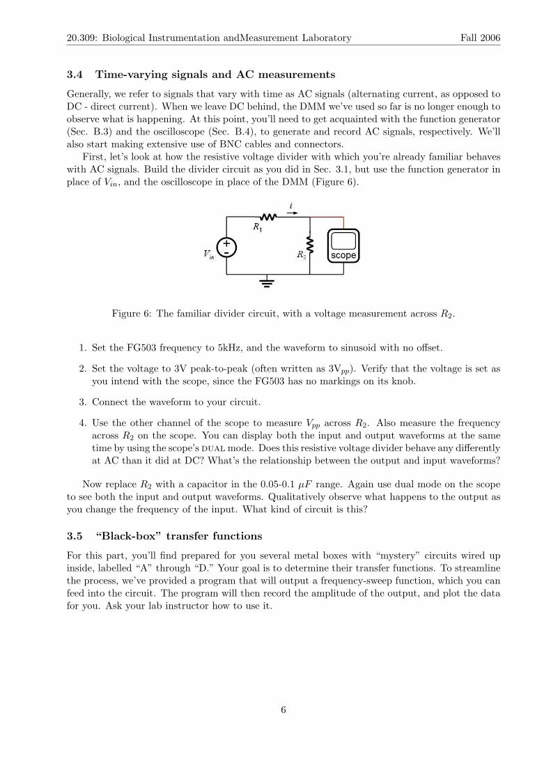
First, let’s look at how the resistive voltage divider with which you’re already familiar behaves with AC signals. Build the divider circuit as you did in Sec. 3.1, but use the function generator in place of Vin, and the oscilloscope in place of the DMM (Figure 6).

Figure 6: The familiar divider circuit, with a voltage measurement across R2.

1. Set the FG503 frequency to 5kHz, and the waveform to sinusoid with no offset.

2. Set the voltage to 3V peak-to-peak (often written as 3Vpp). Verify that the voltage is set as you intend with the scope, since the FG503 has no markings on its knob.

3. Connect the waveform to your circuit.

4. Use the other channel of the scope to measure Vpp across R2. Also measure the frequency across R2 on the scope. You can display both the input and output waveforms at the same time by using the scope’s dual mode. Does this resistive voltage divider behave any differently at AC than it did at DC? What’s the relationship between the output and input waveforms?

Now replace R2 with a capacitor in the 0.05-0.1 µF range. Again use dual mode on the scope to see both the input and output waveforms. Qualitatively observe what happens to the output as you change the frequency of the input. What kind of circuit is this?

3.5 “Black-box” transfer functions

For this part, you’ll find prepared for you several metal boxes with “mystery” circuits wired up inside, labelled “A” through “D.” Your goal is to determine their transfer functions. To streamline the process, we’ve provided a program that will output a frequency-sweep function, which you can feed into the circuit. The program will then record the amplitude of the output, and plot the data for you. Ask your lab instructor how to use it.

6


Appendices

A Circuit Components

A.1 Resistors

The important things to know about resistors are: (1) value, (2) tolerance, and (3) power rating. The power rating indicates the maximum amount of power a resistor can withstand, e.g. 1/4 watt, 1/2 W, etc. The value and the tolerance of the resistor is printed on the package in the form of a color-band code (see below).

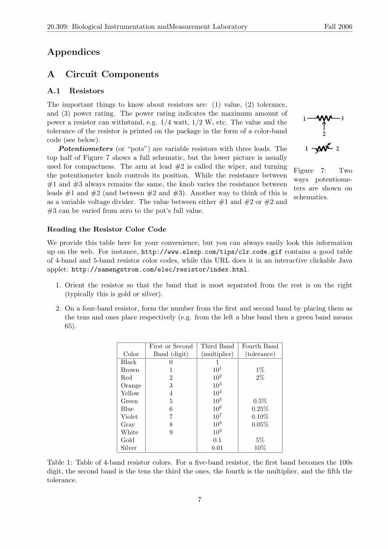
Potentiometers (or “pots”) are variable resistors with three leads. The top half of Figure 7 shows a full schematic, but the lower picture is usually used for compactness. The arm at lead #2 is called the wiper, and turning Figure 7: Two the potentiometer knob controls its position. While the resistance between ways potentiome#1 and #3 always remains the same, the knob varies the resistance between ters are shown on leads #1 and #2 (and between #2 and #3). Another way to think of this is schematics. as a variable voltage divider. The value between either #1 and #2 or #2 and #3 can be varied from zero to the pot’s full value.

Reading the Resistor Color Code

We provide this table here for your convenience, but you can always easily look this information up on the web. For instance, http://www.elexp.com/tips/clr code.gif contains a good table of 4-band and 5-band resistor color codes, while this URL does it in an interactive clickable Java applet: http://samengstrom.com/elec/resistor/index.html.

1. Orient the resistor so that the band that is most separated from the rest is on the right (typically this is gold or silver).

2. On a four-band resistor, form the number from the first and second band by placing them as the tens and ones place respectively (e.g. from the left a blue band then a green band means 65).

First or Second Third Band Fourth Band Color Band (digit) (multiplier) (tolerance)

Black 0 1 Brown 1 101 1% Red 2 102 2% Orange 3 103

Yellow 4 104

Green 5 105 0.5% Blue 6 106 0.25% Violet 7 107 0.10% Gray 8 108 0.05% White 9 109

Gold 0.1 5% Silver 0.01 10%

Table 1: Table of 4-band resistor colors. For a five-band resistor, the first band becomes the 100s digit, the second band is the tens the third the ones, the fourth is the multiplier, and the fifth the tolerance.

7

http://www.elexp.com/tips/clr

http://samengstrom.com/elec/resistor/index.html


3. Multiply the resulting number by the multiplier from the third band (e.g. blue-green-red = 65 × 100 = 6.5kΩ).

4. The most common types of resistors are 5% and 1%, so for quick designation the bodies of these resistors are often color coded (brown – 5% and blue – 1%).

A.2 Capacitors

Capacitors immediately make for much more interesting types of circuits than simple resistive networks, because (1) they can store energy and (2) their behavior is time-dependent.

An intuitive way to think about capacitor behavior is that they are reservoirs for electrical charge, which take time to fill up or empty out. The size of the reservoir (the capacitance C) is one of the factors that determines how quickly or slowly. Because of this, circuits with capacitors in them have time-dependent and frequency-dependent behavior. Capacitors act like open circuits at DC or very low frequencies, and like short circuits at very high frequencies.

A.3 Diodes

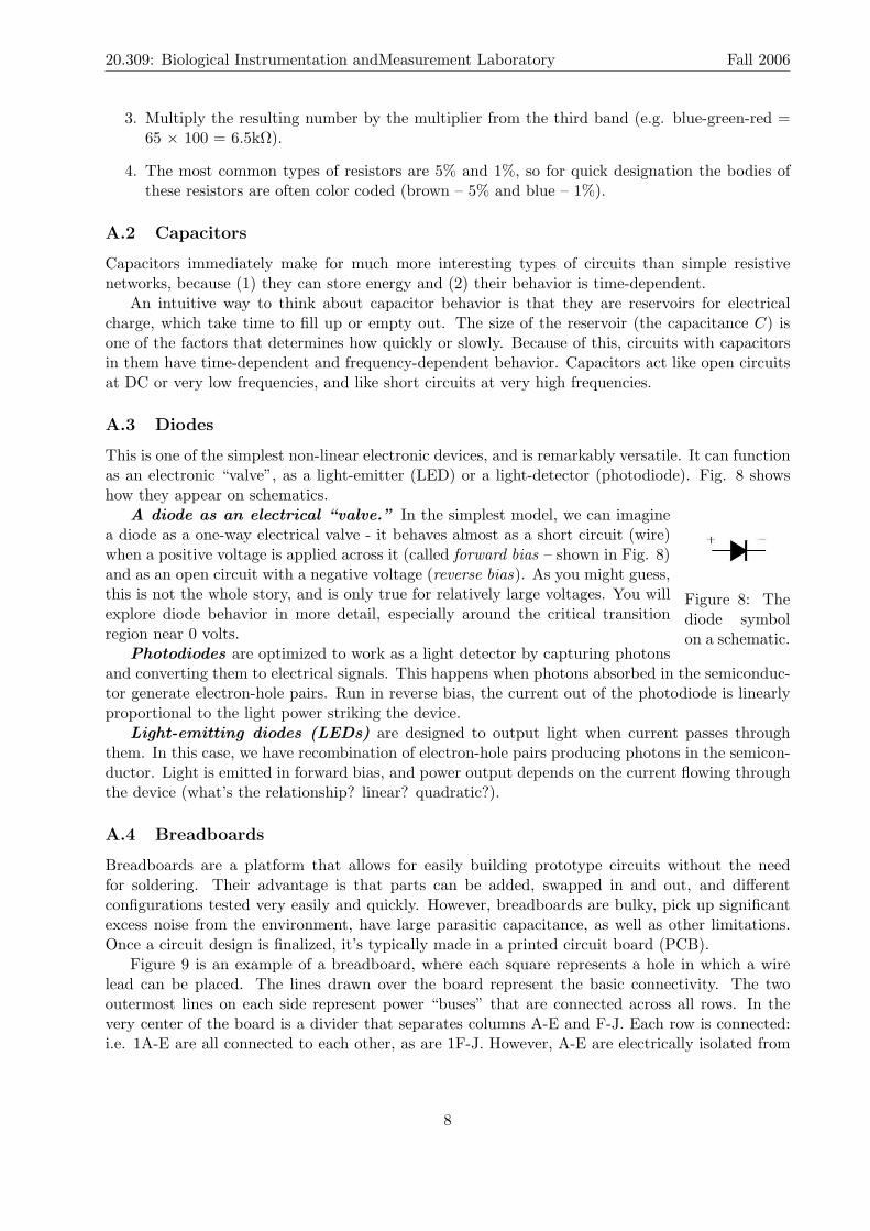
This is one of the simplest non-linear electronic devices, and is remarkably versatile. It can function as an electronic “valve”, as a light-emitter (LED) or a light-detector (photodiode). Fig. 8 shows how they appear on schematics.

A diode as an electrical “valve.” In the simplest model, we can imagine a diode as a one-way electrical valve - it behaves almost as a short circuit (wire) when a positive voltage is applied across it (called forward bias – shown in Fig. 8) and as an open circuit with a negative voltage (reverse bias). As you might guess, this is not the whole story, and is only true for relatively large voltages. You will Figure 8: The explore diode behavior in more detail, especially around the critical transition diode symbol region near 0 volts. on a schematic.

Photodiodes are optimized to work as a light detector by capturing photons and converting them to electrical signals. This happens when photons absorbed in the semiconductor generate electron-hole pairs. Run in reverse bias, the current out of the photodiode is linearly proportional to the light power striking the device.

Light-emitting diodes (LEDs) are designed to output light when current passes through them. In this case, we have recombination of electron-hole pairs producing photons in the semiconductor. Light is emitted in forward bias, and power output depends on the current flowing through the device (what’s the relationship? linear? quadratic?).

A.4 Breadboards

Breadboards are a platform that allows for easily building prototype circuits without the need for soldering. Their advantage is that parts can be added, swapped in and out, and different configurations tested very easily and quickly. However, breadboards are bulky, pick up significant excess noise from the environment, have large parasitic capacitance, as well as other limitations. Once a circuit design is finalized, it’s typically made in a printed circuit board (PCB).

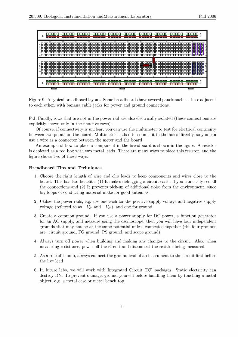
Figure 9 is an example of a breadboard, where each square represents a hole in which a wire lead can be placed. The lines drawn over the board represent the basic connectivity. The two outermost lines on each side represent power “buses” that are connected across all rows. In the very center of the board is a divider that separates columns A-E and F-J. Each row is connected: i.e. 1A-E are all connected to each other, as are 1F-J. However, A-E are electrically isolated from

8


Figure 9: A typical breadboard layout. Some breadboards have several panels such as these adjacent to each other, with banana cable jacks for power and ground connections.

F-J. Finally, rows that are not in the power rail are also electrically isolated (these connections are explicitly shown only in the first five rows).

Of course, if connectivity is unclear, you can use the multimeter to test for electrical continuity between two points on the board. Multimeter leads often don’t fit in the holes directly, so you can use a wire as a connector between the meter and the board.

An example of how to place a component in the breadboard is shown in the figure. A resistor is depicted as a red box with two metal leads. There are many ways to place this resistor, and the figure shows two of these ways.

Breadboard Tips and Techniques

1. Choose the right length of wire and clip leads to keep components and wires close to the board. This has two benefits: (1) It makes debugging a circuit easier if you can easily see all the connections and (2) It prevents pick-up of additional noise from the environment, since big loops of conducting material make for good antennas.

2. Utilize the power rails, e.g. use one each for the positive supply voltage and negative supply voltage (referred to as +Vcc and −Vcc), and one for ground.

3. Create a common ground. If you use a power supply for DC power, a function generator for an AC supply, and measure using the oscilloscope, then you will have four independent grounds that may not be at the same potential unless connected together (the four grounds are: circuit ground, FG ground, PS ground, and scope ground).

4. Always turn off power when building and making any changes to the circuit. Also, when measuring resistance, power off the circuit and disconnect the resistor being measured.

5. As a rule of thumb, always connect the ground lead of an instrument to the circuit first before the live lead.

6. In future labs, we will work with Integrated Circuit (IC) packages. Static electricity can destroy ICs. To prevent damage, ground yourself before handling them by touching a metal object, e.g. a metal case or metal bench top.

9


A.5 Operational Amplifiers

In the upcoming lab module we will start using integrated circuits (ICs) known as operational amplifiers, or op-amps. They are an enormously versatile circuit component, and come in hundreds of special varieties, built to have particular characteristics and trade-offs. We will use some very common general-purpose op-amp, of which a typical example is the LM741.

Every op-amp manufacturer provides a datasheet for every IC they make, and you should always familiarize yourself with it. It provides information on everything from pin and signal connections, to special features, limitations, or applications of a particular IC. We have copies of the datasheets available in the lab for the op-amps we are using, and you’ll want to refer to them regularly as you work.

As you’ll see in lecture, a typical op-amp circuit looks something like Fig. 10. This is called the inverting configuration, because the input is connected to the inverting (–) input. As you might guess, the output signal is the Figure 10: A basic inverting op-amp

negative of the input, times a gain factor set by the circuit. circuit.

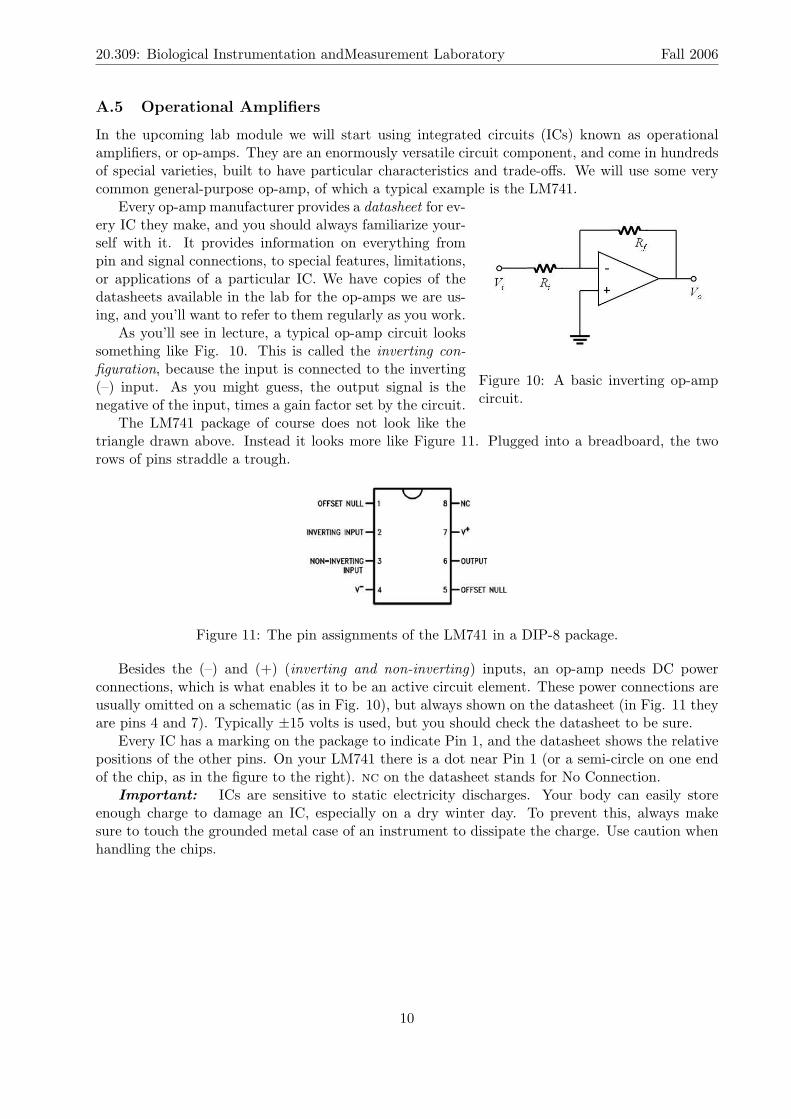
The LM741 package of course does not look like the triangle drawn above. Instead it looks more like Figure 11. Plugged into a breadboard, the two rows of pins straddle a trough.

Figure 11: The pin assignments of the LM741 in a DIP-8 package.

Besides the (–) and (+) (inverting and non-inverting) inputs, an op-amp needs DC power connections, which is what enables it to be an active circuit element. These power connections are usually omitted on a schematic (as in Fig. 10), but always shown on the datasheet (in Fig. 11 they are pins 4 and 7). Typically ±15 volts is used, but you should check the datasheet to be sure.

Every IC has a marking on the package to indicate Pin 1, and the datasheet shows the relative positions of the other pins. On your LM741 there is a dot near Pin 1 (or a semi-circle on one end of the chip, as in the figure to the right). nc on the datasheet stands for No Connection.

Important: ICs are sensitive to static electricity discharges. Your body can easily store enough charge to damage an IC, especially on a dry winter day. To prevent this, always make sure to touch the grounded metal case of an instrument to dissipate the charge. Use caution when handling the chips.

10


B Instruments

The brief descriptions in this section will give you an introduction to each instrument. You can always refer to the manuals available in the lab for more details.

B.1 Digital Multimeter (DMM)

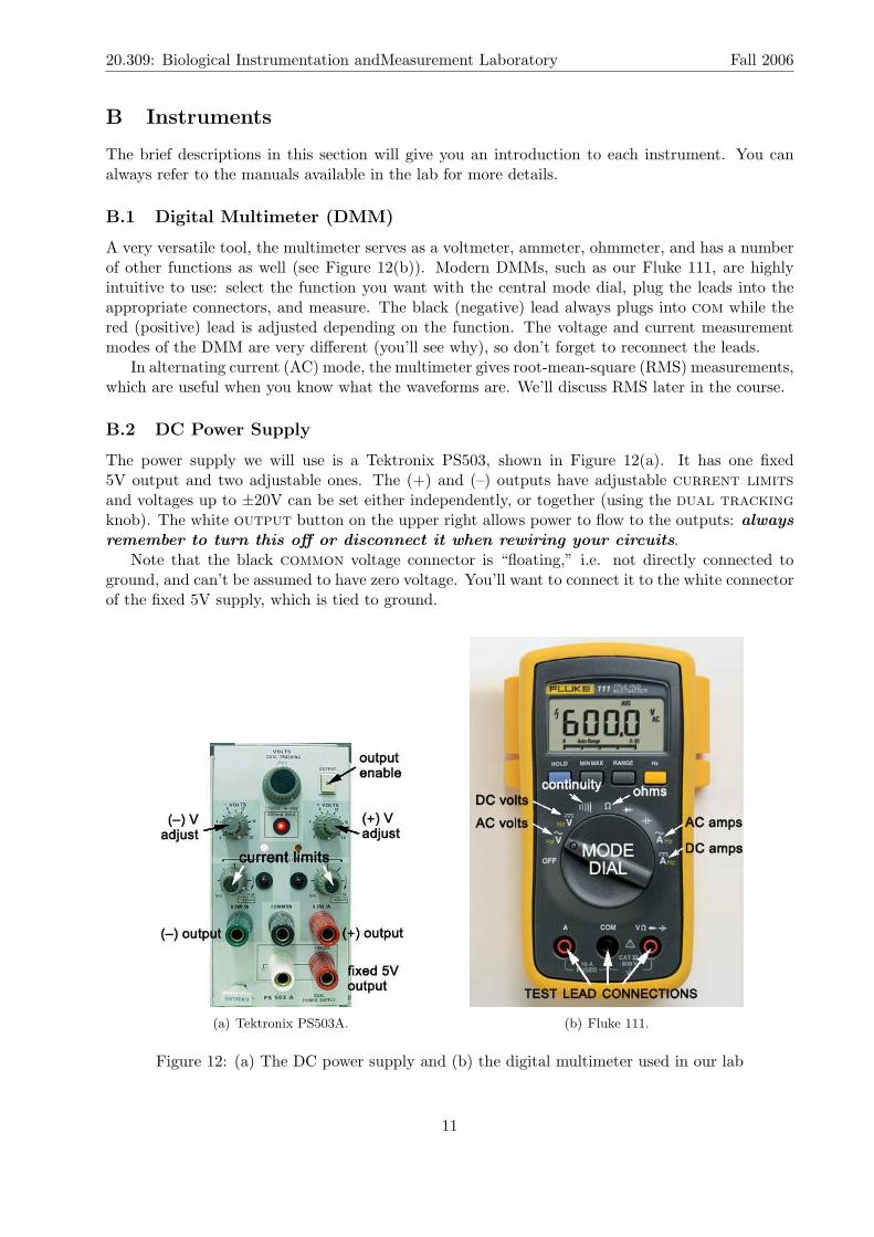
A very versatile tool, the multimeter serves as a voltmeter, ammeter, ohmmeter, and has a number of other functions as well (see Figure 12(b)). Modern DMMs, such as our Fluke 111, are highly intuitive to use: select the function you want with the central mode dial, plug the leads into the appropriate connectors, and measure. The black (negative) lead always plugs into com while the red (positive) lead is adjusted depending on the function. The voltage and current measurement modes of the DMM are very different (you’ll see why), so don’t forget to reconnect the leads.

In alternating current (AC) mode, the multimeter gives root-mean-square (RMS) measurements, which are useful when you know what the waveforms are. We’ll discuss RMS later in the course.

B.2 DC Power Supply

The power supply we will use is a Tektronix PS503, shown in Figure 12(a). It has one fixed 5V output and two adjustable ones. The (+) and (–) outputs have adjustable current limits and voltages up to ±20V can be set either independently, or together (using the dual tracking knob). The white output button on the upper right allows power to flow to the outputs: always remember to turn this off or disconnect it when rewiring your circuits.

Note that the black common voltage connector is “floating,” i.e. not directly connected to ground, and can’t be assumed to have zero voltage. You’ll want to connect it to the white connector of the fixed 5V supply, which is tied to ground.

(a) Tektronix PS503A. (b) Fluke 111.

Figure 12: (a) The DC power supply and (b) the digital multimeter used in our lab

11


B.3 Function Generator

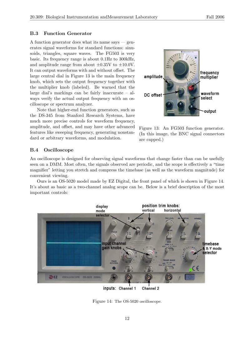
A function generator does what its name says — generates signal waveforms for standard functions: sinusoids, triangles, square waves. The FG503 is very basic. Its frequency range is about 0.1Hz to 300kHz, and amplitude range from about ±0.35V to ±10.0V. It can output waveforms with and without offset. The large central dial in Figure 13 is the main frequency knob, which sets the output frequency together with the multiplier knob (labeled). Be warned that the large dial’s markings can be fairly inaccurate – always verify the actual output frequency with an oscilloscope or spectrum analyzer.

Note that higher-end function generators, such as the DS-345 from Stanford Research Systems, have much more precise controls for waveform frequency, amplitude, and offset, and may have other advanced Figure 13: An FG503 function generator. features like sweeping frequency, generating nonstan- (In this image, the BNC signal connectors dard or arbitrary waveforms, and modulation. are capped.)

B.4 Oscilloscope

An oscilloscope is designed for observing signal waveforms that change faster than can be usefully seen on a DMM. Most often, the signals observed are periodic, and the scope is effectively a “time magnifier” letting you stretch and compress the timebase (as well as the waveform magnitude) for convenient viewing.

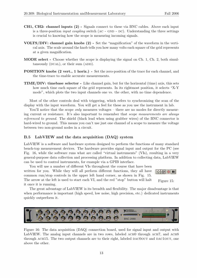
Ours is an OS-5020 model made by EZ Digital, the front panel of which is shown in Figure 14. It’s about as basic as a two-channel analog scope can be. Below is a brief description of the most important controls:

Figure 14: The OS-5020 oscilloscope.

12


CH1, CH2: channel inputs (2) - Signals connect to these via BNC cables. Above each input is a three-position input coupling switch (ac - gnd - dc). Understanding the three settings is crucial to knowing how the scope is measuring incoming signals.

VOLTS/DIV: channel gain knobs (2) - Set the “magnification” of the waveform in the vertical axis. The scale around the knob tells you how many volts each square of the grid represents at a given magnification.

MODE select - Choose whether the scope is displaying the signal on Ch. 1, Ch. 2, both simultaneously (dual), or their sum (add).

POSITION knobs (2 vert., 1 horiz.) - Set the zero-position of the trace for each channel, and the time-trace to enable accurate measurements.

TIME/DIV: timebase selector - Like channel gain, but for the horizontal (time) axis, this sets how much time each square of the grid represents. In its rightmost position, it selects “X-Y mode”, which plots the two input channels one vs. the other, with no time dependence.

Most of the other controls deal with triggering, which refers to synchronizing the scan of the display with the input waveform. You will get a feel for these as you use the instrument in lab.

You’ll notice that the scope only measures voltages – there are no modes for directly measuring current or resistance. It’s also important to remember that scope measurements are always referenced to ground. The shield (black lead when using grabber wires) of the BNC connector is hard-wired to ground. This means you can’t use just one channel of a scope to measure the voltage between two non-ground nodes in a circuit.

B.5 LabVIEW and the data acquisition (DAQ) system

LabVIEW is a software and hardware system designed to perform the functions of many standard bench-top measurement devices. The hardware provides signal input and output for the PC (see Fig. 16, while the software runs what are called “virtual instruments” (VIs), resulting in a very general-purpose data collection and processing platform. In addition to collecting data, LabVIEW can be used to control instruments, for example via a GPIB interface.

You will use a number of different VIs throughout the course that have been written for you. While they will all perform different functions, they all have common run/stop controls in the upper left hand corner, as shown in Fig. 15. The arrow at the left is used to start each VI, and the red ”stop” button will halt Figure 15: it once it is running.

The great advantage of LabVIEW is its breadth and flexibility. The major disadvantage is that when performance is important (high speed, low noise, high precision, etc.) dedicated instruments quickly outperform it.

Figure 16: The data acquisition (DAQ) connection board, used for signal input and output with LabVIEW. The analog input channels are in two rows, labeled ach0 through ach7, and ach8 through ach15. The two output channels are to their right, labeled dac0out and dac1out, one above the other.

13

Documents

Module 0: Introduction to Electronics - MIT OpenCourseWare · 20.309: Biological Instrumentation andMeasurement Laboratory Fall 2006 Module 0: Introduction to Electronics Contents