Munich Personal RePEc Archive

Monetary Policy and Investment

Dynamics: Evidence from Disaggregate

Data

Givens, Gregory and Reed, Robert

University of Alabama

20 January 2015

Online at https://mpra.ub.uni-muenchen.de/61495/

MPRA Paper No. 61495, posted 21 Jan 2015 13:10 UTC

Monetary Policy and Investment Dynamics: Evidence

from Disaggregate Data

Gregory E. Givensa,∗, Robert R. Reeda

aDepartment of Economics, Finance, and Legal Studies, University of Alabama, Tuscaloosa, AL 35487, USA

First Draft: January 2015

Abstract

We use disaggregated data on the components of private fixed investment (PFI) toestimate industry-level responses of real investment and capital prices to unanticipatedmonetary policy. The response functions derive from a restricted large-scale VARestimated over 1959-2007. Our results point to significant cross-sector heterogeneityin the behavior of PFI prices and quantities. For assets belonging to the equipmentcategory of fixed investment, we find that quantities rather than prices absorb most ofthe fallout from a policy shock. By contrast, the price effects tend to be higher andthe output effects lower for nonresidential structures.

Keywords: Investment, Monetary policy, Disaggregate data, VAR

JEL Classification: E22, E32, E52

∗Corresponding author. Tel.: + 205 348 8961.E-mail address: gegivens@cba.ua.edu (G.E. Givens).

1 Introduction

How quickly and to what extent monetary policy influences economic conditions varies from

one sector of the economy to another. This makes the task of central banking difficult because

the impetus for policy intervention depends on the source of weakness or instability in the

market. The 2001 recession, for example, was accompanied by declining private expenditures

on capital equipment. The press release following the January 31, 2001 meeting of the Federal

Open Market Committee (FOMC) stated that “business spending on capital equipment [has]

weakened appreciably.” The recession of 2007-2009, on the other hand, was greatly intensified

by a collapse in residential investment. Official policy statements published after the August

5, 2008 FOMC meeting proclaimed that “the ongoing housing contraction . . . [is] likely to

weigh on economic growth over the next few quarters.”

Given the status that investment-related activity has in FOMC deliberations, this paper

empirically examines how conditions across all the private fixed investment categories re-

ported by the Bureau of Economic Analysis (BEA) respond to aggregate monetary shocks.

To date, there are a total of 67 distinct fixed investment types represented in the data

that underlie the National Income and Product Accounts (NIPA). Some examples include

commercial warehouses, lodgings, mining and oilfield machinery, railroad equipment, and

single-family housing.1 For each one of these industry groups, the BEA publishes quarterly

data on both nominal expenditures and the price level. Our main goal here is to document

potential cross-sector differences in the response of these disaggregated series to unantici-

pated monetary policy. We focus on exposing asymmetries not only in the magnitude of the

price and quantity responses, but also in the speed with which policy actions are transmitted

to the many diverse capital-goods producing industries. An analysis of the cross-sectional

results also allows us to see if there are any systematic relationships among prices and quan-

1See Table A in the appendix for a complete list of the separate components of private fixed investment.

1

tities within more broadly-defined asset categories like residential structures, nonresidential

structures, and durable equipment. Our findings can therefore provide evidence on whether

market conditions in related industries react similarly to aggregate shocks.

The notion that monetary policy affects various sectors of the economy differently is

not new. There is a large body of research that studies the impact of policy disturbances

on a wide range of disaggregated prices and quantities, and the results overwhelmingly

point to sizable and significant cross-sector heterogeneity. Lastrapes (2006) and Balke and

Wynne (2007) demonstrate that policy shocks alter the distribution of prices comprising the

numerous industry components of the Producer Price Index. The authors interpret these

relative price movements as evidence of monetary nonneutrality. Bils, Klenow, and Kryvtsov

(2003) and Altissimo, Mojon, and Zaffaroni (2009) draw similar conclusions for the major

retail price categories found in the US and euro area Consumer Price Index, respectively.2

Using industry-level data, Barth and Ramey (2002), Dedola and Lippi (2005), and Loo and

Lastrapes (1998) report substantial heterogeneity in sectoral output responses to a monetary

shock. Carlino and Defina (1998) examine the policy effects on real personal income in the

eight BEA regions of the United States. They find evidence of asymmetry in the response

patterns and trace this result to differences in certain industry characteristics across regions.

Despite the many contributions that deal with the sectoral effects of monetary policy, the

literature is largely silent on whether changes in policy influence the various types of invest-

ment activity differently.3 The reason is that existing empirical studies emphasize aggregate

investment and disregard information contained in disaggregate data (e.g., Bernanke and

Gertler, 1995; Christiano, Eichenbaum, and Evans, 1999). Our paper aims to fill this void,

and by doing so, contributes to the policy discussion in two ways. First, central banks want

2In a related set of papers, Clark (2006), Boivin, Giannoni, and Mihov (2009), and Baumeister, Liu, andMumtaz (2013) use disaggregate data to assess differences between aggregate and sectoral inflation dynamics.Enders and Ma (2011) show that the volatility declines experienced during the so-called Great Moderationera did not occur simultaneously across all sectors of the US economy.

3Recent theoretical contributions include Erceg and Levin (2006) and Barsky, House, and Kimball (2007).

2

to know how their actions affect conditions across the full spectrum of capital-producing

industries. Our results help inform policymakers by exposing differences in the response to a

monetary shock among all the major investment categories represented in the NIPA. Second,

the stylized facts that emerge from this study can serve as benchmarks for developing and

evaluating more comprehensive models of the monetary transmission mechanism.

To obtain the responses of industry-level prices and quantities, we employ a quarterly

structural vector autoregression (VAR) and identify monetary shocks as orthogonalized in-

novations to the federal funds rate. Our estimation period is 1959 to 2007. As first shown

by Sims (1992) and Bernanke and Blinder (1992), the VAR is a convenient framework for es-

timating the dynamic effects of monetary policy innovations. To maintain sufficient degrees

of freedom, however, estimated VARs typically involve a limited number of macroeconomic

variables. Incorporating a broad panel of disaggregated investment data would obviously

violate this practice and, absent restrictions on the model, make estimation infeasible for

any suitable lag choice. In this paper we avoid problems associated with most large-scale

VARs by adopting an empirical strategy used by Barth and Ramey (2002) and formalized in

Lastrapes (2005). The procedure calls for segmenting the VAR into two blocks, the first con-

taining macroeconomic aggregates or ‘common factors’ and the second containing industry

variables. Degrees of freedom are preserved by assuming (i) common factors are independent

of the industry block and (ii) variables in the latter subset are mutually independent after

conditioning on the former. Under these conditions least squares is efficient and monetary

policy innovations can be identified through restrictions on just the macro-variable equations.

Estimation results show that policy outcomes are not uniform across capital-producing

industries. While most, but not all, prices and quantities increase after a policy expansion,

there is significant cross-sectional variation in the size and speed of the adjustment paths.

The implication is that monetary policy has distributional effects, not only on the com-

position of fixed investment but also on the dispersion of relative prices. A more focused

3

comparison among certain industry groups, however, reveals similarities in the way some

prices and quantities interact over time. For example, where prices of durable equipment of-

ten react slowly to a policy shock, production volumes tend to respond swiftly. By contrast,

producers of nonresidential structures usually raise prices in the short run rather than adjust

quantities. In markets for residential structures, the expansionary effects of policy show up

almost immediately in both prices and quantities.

2 Investment Data

Source data on nominal expenditures and price indexes for all categories of private fixed

investment (PFI) come from the Underlying Detail Tables for Gross Domestic Product re-

ported (online) by the BEA.4 The tables disassemble PFI into various components, the num-

ber of which differ by level of aggregation. There are only two components reported at the

highest aggregation level, residential and nonresidential investment. The former comprises

residential investment in structures and equipment while the latter consists of nonresiden-

tial structures, equipment, and a third group encompassing items described as intellectual

property products.5 The underlying data decompose PFI further into 16 separate subcate-

gories covering more narrowly-defined sectors of the economy. This third level of aggregation

includes series such as commercial and health care buildings, transportation equipment, soft-

ware, and permanent-site residential structures. Sinking even further in the detailed NIPA

estimates reveals as many as 67 individual series spanning all of PFI. They represent the

most disaggregate measures available in the underlying data, and most of them summarize

investment activity within a specific industry. Some examples include food and beverage

establishments, religious structures, photocopy equipment, farm tractors, and dormitories.

4http://www.bea.gov/iTable/index UD.cfm/5Intellectual property products were grouped and re-classified as a component of nonresidential fixed

investment as part of the comprehensive revision to the NIPA in July of 2013.

4

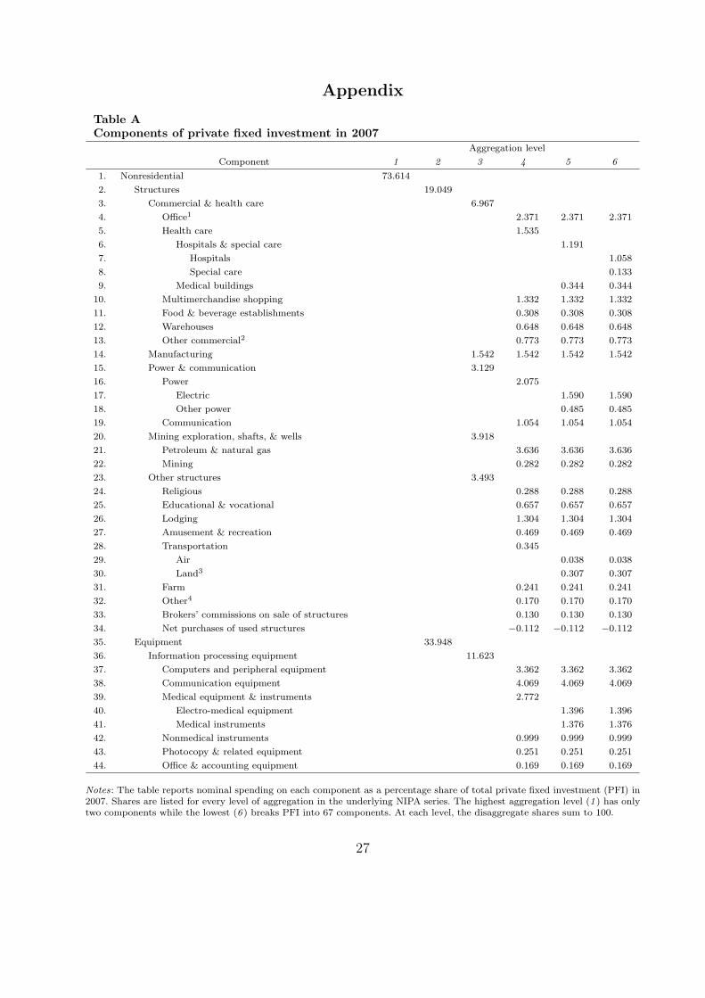
Table A in the appendix lists all of the component series of PFI and organizes them accord-

ing to aggregation level. The table also reports nominal spending on each disaggregate as a

percentage share of total private fixed investment in 2007.

The estimation exercises carried out in this paper employ a panel of investment data

assembled at the most detailed aggregation level published by the BEA. The panel consists

of disaggregate price and quantity series for the numerous components listed in Table A.

In the majority of cases, data on these measures are available on a quarterly basis from

1959 through the present. A small number of these series, however, were excluded from

the analysis because of missing observations. In such instances, the offending series were

replaced by data from the next lowest level of aggregation.6 This left us with a total of 64

disaggregate series on PFI prices and an equal number of series on nominal investment. The

set of variables omitted from our panel represented just 3.4% of PFI expenditures in 2007.7

3 Empirical Framework

We are interested in characterizing the effects of exogenous monetary shocks on the cross-

sectional variation among investment prices and real investment spending. Following in the

tradition of Bernanke and Blinder (1992) and Christiano et al. (1999), we employ a vector

autoregression and identify monetary shocks as innovations to the federal funds rate.

One complication that emerges from our use of disaggregate data concerns the large

dimensionality of a VAR that includes, among other variables, 128 different PFI prices and

quantities. Without placing additional restrictions on the model, insufficient observations

and a loss of degrees of freedom make estimation infeasible. To address this problem, we

6Separate data on light trucks, including utility vehicles, and other trucks, buses, and truck trailers (lines56 and 57 of Table A) are not available before 1987. We therefore replace these series with aggregate dataon trucks, buses, and truck trailers (line 55), which appear without interruption from 1959 on.

7The BEA does not compute price indexes for net purchases of used residential or nonresidential structures(lines 34 and 93 of Table A). Both quantities are therefore excluded from the panel.

5

borrow from Barth and Ramey (2002) and Lastrapes (2005) by partitioning the variables

into two blocks. The first block consists of macroeconomic variables or ‘common factors’ that

appear regularly in the monetary VAR literature. It includes real gross domestic product

(GDP), the GDP chain-type price index (P), total private fixed investment (PFI), the deflator

for private fixed investment (Q), the ratio of crude materials to finished goods in the Producer

Price Index (PCM), the effective federal funds rate (FFR), and the ratio of nonborrowed to

total reserves (NTR).8 The second block consists of only two equations at a time, one for the

disaggregate price series of interest and the other for its corresponding real quantity. Efficient

estimation and consistent identification of the FFR shock can be obtained by imposing

exclusion restrictions on the set of coefficients in the macro-variable equations that govern

feedback from the disaggregate series. This ensures that common factors are independent of

the industry variables since the feedback coefficients of the former are fixed across regressions.

Coefficients of the disaggregate series are permitted to vary with each industry examined.9

The relationship between aggregate and industry variables can be seen more clearly by

considering the VAR process

Zt = µ+ A(L)Zt−1 + ϵt, (1)

where Z ′

t = [GDPt Pt PFIt Qt PCMt FFRt NTRt ij,t qj,t], µ is a vector of constants, A(L)

is a conformable lag polynomial of finite order, and the error term ϵt ∼ i.i.d. (0,Ω). The

quantities ij,t and qj,t denote real spending and the price deflator, respectively, on investment

goods from industry j. Independence of the first seven variables from ij,t and qj,t is obtained

8We include the relative price of crude materials in order to mitigate the “price puzzle,” a temporarydeflation following a negative funds rate shock. Sims (1992) points out that such inconsistencies are theresult of omitting variables from the VAR that provide information on expected future inflation.

9Using similar restrictions to estimate sectoral responses to oil shocks, Davis and Haltiwanger (2001)argue that the resultant system is equivalent to a pseudo-panel-data VAR.

6

by imposing restrictions on the lag polynomial of the form

A9×9

(k) =

A1,17×7

(k) 07×2

A2,12×7

(k) A2,22×2

(k)

for all k lags. These restrictions imply that macroeconomic aggregates are unaffected by

variations in the disaggregate series. It follows that estimation and identification of monetary

shocks will be the same regardless of which price-quantity industry pair is used in the VAR.

By including only one (ij,t, qj,t) combination at a time, we are also assuming that the full

set of investment prices and quantities are mutually independent after conditioning on the

first seven common factors. Thus any observed correlation across industries is accounted for

by their joint dependence on the aggregate macro variables. Had we expanded Zt to consider

all industries simultaneously, the assumption of mutual independence would impose a block-

diagonal structure on the matrix A2,2(k) (a 128×128 object in this case) for all k lags. That

is to say, each pair of (ij,t, qj,t) equations would contain only its own lagged values as well as

lags of the common factors. This is equivalent to estimating our 9-variable system separately

for each industry category while leaving the 2×2 partitions A2,2(k) completely unrestricted.

To identify monetary shocks, we adopt the recursiveness approach described in Chris-

tiano et al. (1999). The procedure begins by specifying a relationship between structural

disturbances (νt) and reduced-form errors (ϵt) of the form ϵt = Sνt, where S is a 9 × 9

contemporaneous matrix. It follows that (1) can be written in terms of structural shocks as

Zt = B(L) (µ+ Sνt) , (2)

where B(L) ≡ (I − A(L)L)−1 is a convergent infinite-order lag polynomial. Here monetary

shocks are interpreted as structural innovations to the federal funds rate, corresponding to

the sixth element of νt in the transformed system (2). The impulse responses of Zt to a

7

policy shock are summarized by the matrix polynomial B(L)S.

The elements of B(L) and S are estimated in two steps. First, we use ordinary least

squares on (1) to obtain estimates of A(L) and ϵt. We then impose orthogonality and normal-

ization (unit variance) restrictions on the covariance matrix of νt along with triangular restric-

tions on the matrix S. This allows us to identify S from a standard Choleski decomposition

of Ω. Given estimates of A(L), estimates of B(L) are derived from B(L) = (I − A(L)L)−1.

Imposing a lower triangular structure on S is motivated by assumptions regarding time

lags in the transmission of monetary shocks to the broader economy. One assumption is

that the common factors appearing above FFRt in (1) react to a policy innovation with a

one-quarter delay. These restrictions are met by inserting zeros in the first five elements of

the sixth column of S. A second assumption is that variables below the funds rate may react

contemporaneously (within the same quarter) to an FFR shock. The last four coefficients in

the sixth column of S are therefore kept free. Note that by ordering ij,t and qj,t last, we are

assuming monetary shocks can affect industry variables before they affect the macro variables

(excluding NTR).10 No additional timing restrictions are needed to achieve identification.11

The dataset consists of quarterly observations covering 1959:Q1 to 2007:Q4.12 All series

except FFRt are expressed in natural-log levels. Real investment spending for industry j

is the ratio of nominal expenditures to the industry price index described in the previous

section. Finally, four lags of each variable are used in estimating (1). We found this number

was sufficient to stamp out the serial correlation in both macro and industry-level residuals.13

10An alternative view is that policy shocks should affect both macro and industry-level variables no soonerthan with a one-quarter lag. In this case ij,t and qj,t must be positioned above FFRt in (1). It turns out thatsuch a re-ordering has little effect on our main quantitative results since the large majority of impact-periodresponses of the industry variables are not significantly different from zero (see Fig. 3).

11As shown by Christiano et al. (1999), the set of response functions are invariant to the specific orderingof variables within the two groups above and below the funds rate.

12We exclude dates covering the financial crisis and recovery. During this period, nonborrowed reserves be-came negative due to injections of borrowed reserves through the Term Auction Facility. This is problematicfor estimation since the relevant variable is the natural log of the ratio of nonborrowed to total reserves.

13Ljung-Box Q tests fail to reject the hypothesis of no serial correlation in the residuals at the 5% level.

8

4 Empirical Findings

4.1 Aggregate Responses to a Policy Shock

Before commenting on the industry response functions, we verify that our estimated VAR

generates aggregate dynamics consistent with known findings. Fig. 1 plots impulse responses

for GDPt, Pt, PCMt, FFRt, and NTRt to a one standard deviation (71 basis point) drop in

the federal funds rate. Shaded regions correspond to 90 percent confidence bands.14

The aggregate effects of an expansionary FFR innovation can be summarized as follows.

First, there is a persistent decline in the funds rate accompanied by a large and persistent

increase in the ratio of nonborrowed to total reserves. Estimates suggest that it takes over

a year for both quantities to return to pre-shock levels. Second, real GDP exhibits the

usual hump-shaped pattern seen in numerous empirical studies (e.g., Leeper, Sims, and Zha,

1996). Here we find that it reaches a peak of 0.65 percent roughly six quarters after the shock.

Third, after a delay of five quarters, the chain-type price index for GDP starts climbing to

a permanently higher level. Four years after the shock, however, it is still only 0.64 percent

above the baseline. Results showing that aggregate prices respond sluggishly to a policy

shock appear frequently in the VAR literature (e.g., Christiano et al., 1999). Fourth, a funds

rate shock generates a large and sustained increase in the relative price of crude materials.

The maximum impact is nearly 2 percent and occurs at a horizon of three years.

14Confidence bands are computed using Monte Carlo methods. We first take the joint distribution of theVAR coefficients and the residual covariance matrix to be asymptotically normal with mean equaling thesample estimates and covariance equaling the sample covariance matrix of those estimates. We then draw10, 000 random vectors from this normal distribution and, preserving the identification restrictions, computeimpulse response functions for each draw. Ninety percent confidence bands correspond to the 5th and 95th

percent bounds of the simulated distribution of impulse response functions over all 10, 000 trials.

9

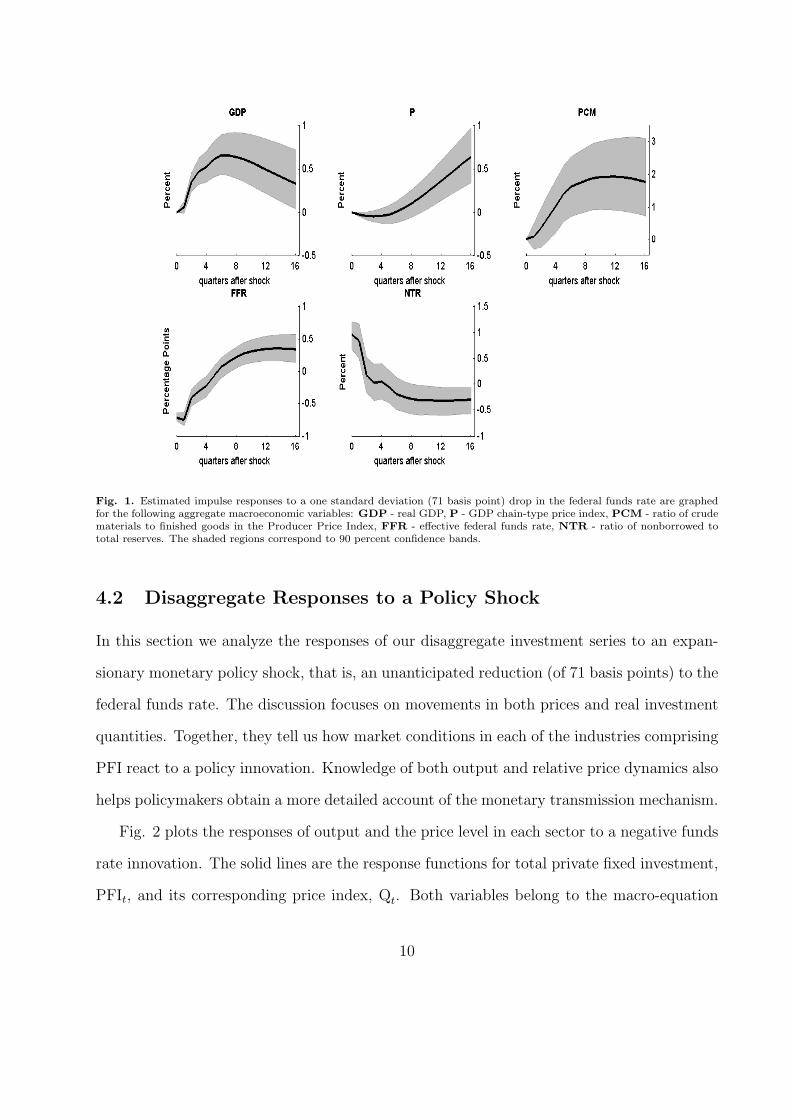
Fig. 1. Estimated impulse responses to a one standard deviation (71 basis point) drop in the federal funds rate are graphedfor the following aggregate macroeconomic variables: GDP - real GDP, P - GDP chain-type price index, PCM - ratio of crudematerials to finished goods in the Producer Price Index, FFR - effective federal funds rate, NTR - ratio of nonborrowed tototal reserves. The shaded regions correspond to 90 percent confidence bands.

4.2 Disaggregate Responses to a Policy Shock

In this section we analyze the responses of our disaggregate investment series to an expan-

sionary monetary policy shock, that is, an unanticipated reduction (of 71 basis points) to the

federal funds rate. The discussion focuses on movements in both prices and real investment

quantities. Together, they tell us how market conditions in each of the industries comprising

PFI react to a policy innovation. Knowledge of both output and relative price dynamics also

helps policymakers obtain a more detailed account of the monetary transmission mechanism.

Fig. 2 plots the responses of output and the price level in each sector to a negative funds

rate innovation. The solid lines are the response functions for total private fixed investment,

PFIt, and its corresponding price index, Qt. Both variables belong to the macro-equation

10

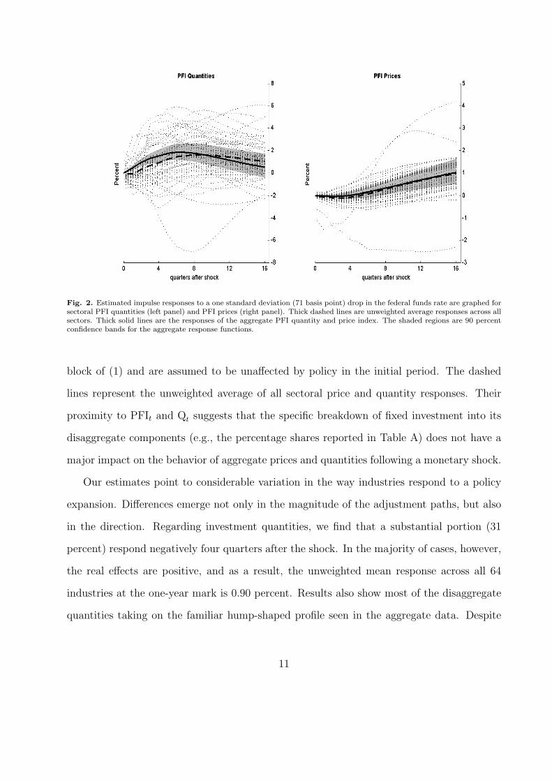
Fig. 2. Estimated impulse responses to a one standard deviation (71 basis point) drop in the federal funds rate are graphed forsectoral PFI quantities (left panel) and PFI prices (right panel). Thick dashed lines are unweighted average responses across allsectors. Thick solid lines are the responses of the aggregate PFI quantity and price index. The shaded regions are 90 percentconfidence bands for the aggregate response functions.

block of (1) and are assumed to be unaffected by policy in the initial period. The dashed

lines represent the unweighted average of all sectoral price and quantity responses. Their

proximity to PFIt and Qt suggests that the specific breakdown of fixed investment into its

disaggregate components (e.g., the percentage shares reported in Table A) does not have a

major impact on the behavior of aggregate prices and quantities following a monetary shock.

Our estimates point to considerable variation in the way industries respond to a policy

expansion. Differences emerge not only in the magnitude of the adjustment paths, but also

in the direction. Regarding investment quantities, we find that a substantial portion (31

percent) respond negatively four quarters after the shock. In the majority of cases, however,

the real effects are positive, and as a result, the unweighted mean response across all 64

industries at the one-year mark is 0.90 percent. Results also show most of the disaggregate

quantities taking on the familiar hump-shaped profile seen in the aggregate data. Despite

11

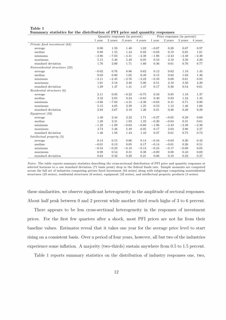
Table 1Summary statistics for the distribution of PFI price and quantity responses

Quantity responses (in percent) Price responses (in percent)

1 year 2 years 3 years 4 years 1 year 2 years 3 years 4 years

Private fixed investment (64)

average 0.90 1.59 1.40 1.02 −0.07 0.28 0.67 0.97

median 0.88 1.55 1.44 0.92 −0.03 0.19 0.65 1.01

minimum −3.86 −7.03 −4.31 −2.38 −1.96 −2.43 −2.49 −2.30

maximum 5.15 5.46 5.49 6.05 0.53 2.10 3.50 4.20

standard deviation 1.76 2.00 1.71 1.60 0.36 0.61 0.76 0.77

Nonresidential structures (23)

average −0.02 0.76 0.86 0.62 0.12 0.62 1.18 1.45

median 0.03 0.80 1.05 0.49 0.15 0.62 1.03 1.36

minimum −3.11 −2.45 −2.76 −2.22 −0.33 0.08 0.61 0.85

maximum 1.61 3.18 3.40 5.00 0.51 2.10 3.50 4.20

standard deviation 1.29 1.47 1.41 1.47 0.17 0.36 0.54 0.61

Residential structures (6)

average 2.11 0.95 −0.22 −0.75 0.33 0.85 1.18 1.37

median 3.32 2.05 0.24 −0.83 0.40 0.93 1.24 1.45

minimum −3.86 −7.03 −4.31 −2.38 −0.03 0.41 0.71 0.90

maximum 5.15 4.05 2.39 1.25 0.53 1.12 1.46 1.66

standard deviation 2.94 3.67 2.10 1.26 0.21 0.26 0.28 0.29

Equipment (32)

average 1.40 2.44 2.22 1.71 −0.27 −0.05 0.29 0.60

median 1.28 2.31 1.93 1.23 −0.20 −0.04 0.31 0.61

minimum −1.32 −1.09 −0.63 −0.60 −1.96 −2.43 −2.49 −2.30

maximum 4.74 5.46 5.49 6.05 0.17 2.03 2.86 2.37

standard deviation 1.46 1.56 1.44 1.43 0.37 0.61 0.75 0.72

Intellectual property (3)

average 0.14 0.15 0.06 0.14 −0.16 −0.03 0.20 0.42

median −0.01 0.13 0.05 0.17 −0.14 −0.01 0.26 0.51

minimum −0.54 −0.23 −0.18 −0.13 −0.24 −0.17 −0.09 0.05

maximum 0.98 0.54 0.31 0.38 −0.09 0.08 0.43 0.69

standard deviation 0.63 0.32 0.20 0.21 0.06 0.10 0.22 0.27

Notes: The table reports summary statistics describing the cross-sectional distribution of PFI price and quantity responses atselected horizons to a one standard deviation (71 basis point) drop in the federal funds rate. Sample moments are computedacross the full set of industries comprising private fixed investment (64 series) along with subgroups comprising nonresidentialstructures (23 series), residential structures (6 series), equipment (32 series), and intellectual property products (3 series).

these similarities, we observe significant heterogeneity in the amplitude of sectoral responses.

About half peak between 0 and 2 percent while another third reach highs of 3 to 6 percent.

There appears to be less cross-sectional heterogeneity in the responses of investment

prices. For the first few quarters after a shock, most PFI prices are not far from their

baseline values. Estimates reveal that it takes one year for the average price level to start

rising on a consistent basis. Over a period of four years, however, all but two of the industries

experience some inflation. A majority (two-thirds) sustain anywhere from 0.5 to 1.5 percent.

Table 1 reports summary statistics on the distribution of industry responses one, two,

12

three, and four years after the occurrence of a policy shock. Across all categories of private

fixed investment we see that the dispersion in quantities, as measured by standard deviation,

is greater than the dispersion in prices at each horizon. The spread of output responses

reaches its highest point about eight quarters after the shock, with half of all industries

having increased anywhere from 1.55 to 5.46 percent. By comparison, price dispersion is

smaller and increases gradually for the first few years. The standard deviation is only 0.36

percent one year after the shock but rises to 0.77 percent by the end of year four. It is also

interesting to note that while the distribution of responses continually shifts towards higher

average prices, the variance of that distribution levels off three years after the shock.

Whether price and quantity dispersion is a compelling feature of the data depends to some

extent on the significance of the estimates displayed in Fig. 2. To assess significance, we

follow Balke and Wynne (2007) by recording the fraction of disaggregate responses that are

statistically different from zero at the 10 percent level. A response is considered significant

if at least 90 percent of the simulated responses, obtained by sampling from the normal

distribution described in footnote 14, are either strictly positive or strictly negative. The

results are illustrated in Fig. 3. At horizons of two quarters or less, the fraction of statistically

significant output responses never exceeds 25 percent. The proportion increases to around

60 percent seven quarters after the shock and reverts back to 20 percent by the four-year

mark. Regarding PFI prices, barely 14 percent are significant one quarter after the policy

shock, but over 50 percent are significant six quarters later. By the end of the fourth year,

as many as 80 percent of industry prices are statistically different from pre-shock levels.

That a large share of disaggregate responses are significant bolsters the argument made

by some that monetary nonneutralities are present in the capital-goods sector of the US

economy. Should one’s goal be to identify the underlying sources of nonneutrality, the

results of our VAR analysis could in principle be used to evaluate the likelihood of alternative

models (e.g., price rigidity, imperfect information, limited participation). Here our objective

13

0 2 4 6 8 10 12 14 160.0

0.1

0.2

0.3

0.4

0.5

0.6

0.7

0.8

0.9

1.0Fraction of Significant PFI Price and Quantity Responses

quarters after shock

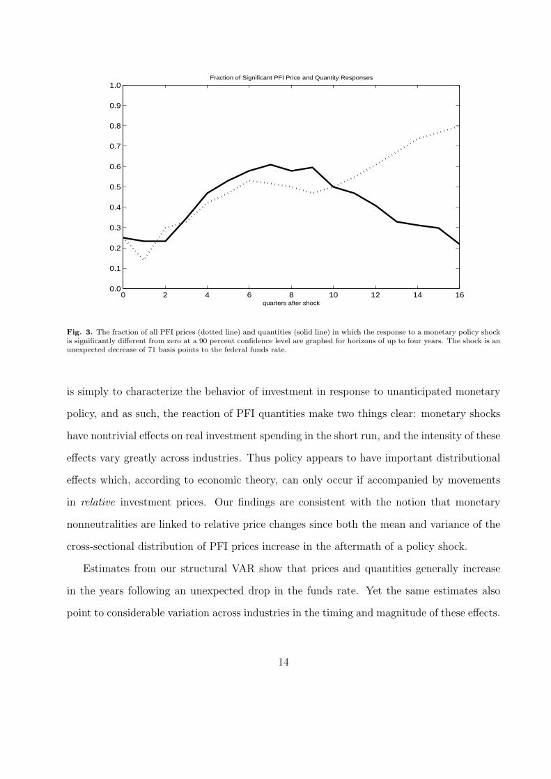
Fig. 3. The fraction of all PFI prices (dotted line) and quantities (solid line) in which the response to a monetary policy shockis significantly different from zero at a 90 percent confidence level are graphed for horizons of up to four years. The shock is anunexpected decrease of 71 basis points to the federal funds rate.

is simply to characterize the behavior of investment in response to unanticipated monetary

policy, and as such, the reaction of PFI quantities make two things clear: monetary shocks

have nontrivial effects on real investment spending in the short run, and the intensity of these

effects vary greatly across industries. Thus policy appears to have important distributional

effects which, according to economic theory, can only occur if accompanied by movements

in relative investment prices. Our findings are consistent with the notion that monetary

nonneutralities are linked to relative price changes since both the mean and variance of the

cross-sectional distribution of PFI prices increase in the aftermath of a policy shock.

Estimates from our structural VAR show that prices and quantities generally increase

in the years following an unexpected drop in the funds rate. Yet the same estimates also

point to considerable variation across industries in the timing and magnitude of these effects.

14

−2 −1 0 1−4

−2

0

2

4

6

Responses of PFI prices after 1 year

Res

pons

es o

f P

FI q

uant

ities

afte

r 1

year

−4 −2 0 2 4−10

−5

0

5

10

Responses of PFI prices after 2 years

Res

pons

es o

fP

FI q

uant

ities

afte

r 2

year

s

−4 −2 0 2 4−5

0

5

10

Responses of PFI prices after 3 years

Res

pons

es o

f P

FI q

uant

ities

afte

r 3

year

s

Cross−sectional regression line:

IRF(ij,t

) = α + β × IRF(qj,t

) + ej,t

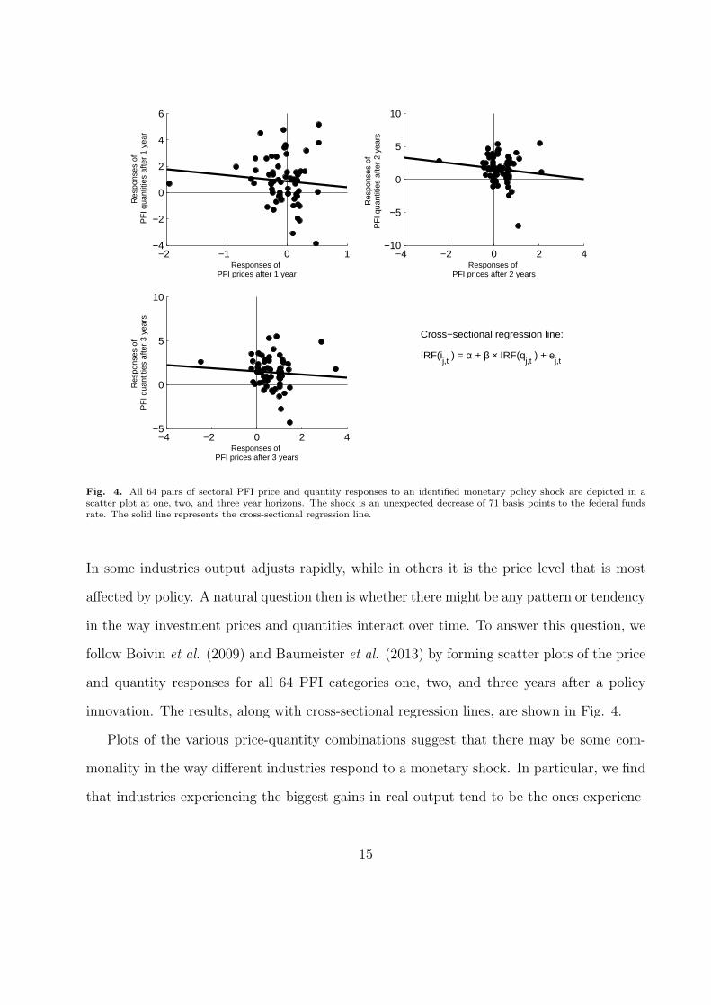
Fig. 4. All 64 pairs of sectoral PFI price and quantity responses to an identified monetary policy shock are depicted in ascatter plot at one, two, and three year horizons. The shock is an unexpected decrease of 71 basis points to the federal fundsrate. The solid line represents the cross-sectional regression line.

In some industries output adjusts rapidly, while in others it is the price level that is most

affected by policy. A natural question then is whether there might be any pattern or tendency

in the way investment prices and quantities interact over time. To answer this question, we

follow Boivin et al. (2009) and Baumeister et al. (2013) by forming scatter plots of the price

and quantity responses for all 64 PFI categories one, two, and three years after a policy

innovation. The results, along with cross-sectional regression lines, are shown in Fig. 4.

Plots of the various price-quantity combinations suggest that there may be some com-

monality in the way different industries respond to a monetary shock. In particular, we find

that industries experiencing the biggest gains in real output tend to be the ones experienc-

15

ing the smallest growth in prices. Conversely, price increases are usually higher in sectors

where output growth is lower. Our results also show this relationship to be persistent, which

explains why the cross-sectional regression lines are negatively sloped at each response hori-

zon. Point estimates of these slope coefficients, however, should be interpreted with a great

deal of caution. Although they range from −0.45 after one year to −0.17 after three years,

none are statistically significant at regular confidence levels. Thus evidence of a consistent

inverse relationship between the magnitudes of our price and quantity responses is somewhat

limited when looking across all industry components of private fixed investment. In the next

section, we examine whether the evidence is any more convincing for sample groups that

include only those industries belonging to more narrowly-defined subcategories of PFI.

4.3 Major Components of Fixed Investment

To determine whether conditions across certain industry groups react similarly to a policy

innovation, we organize the sectoral price and quantity responses into four major investment

subcategories: nonresidential structures, residential structures, durable equipment, and in-

tellectual property products. Of the 64 PFI components included in our sample, the BEA

classifies 23 as nonresidential structures, 6 as residential structures, 32 as equipment, and 3

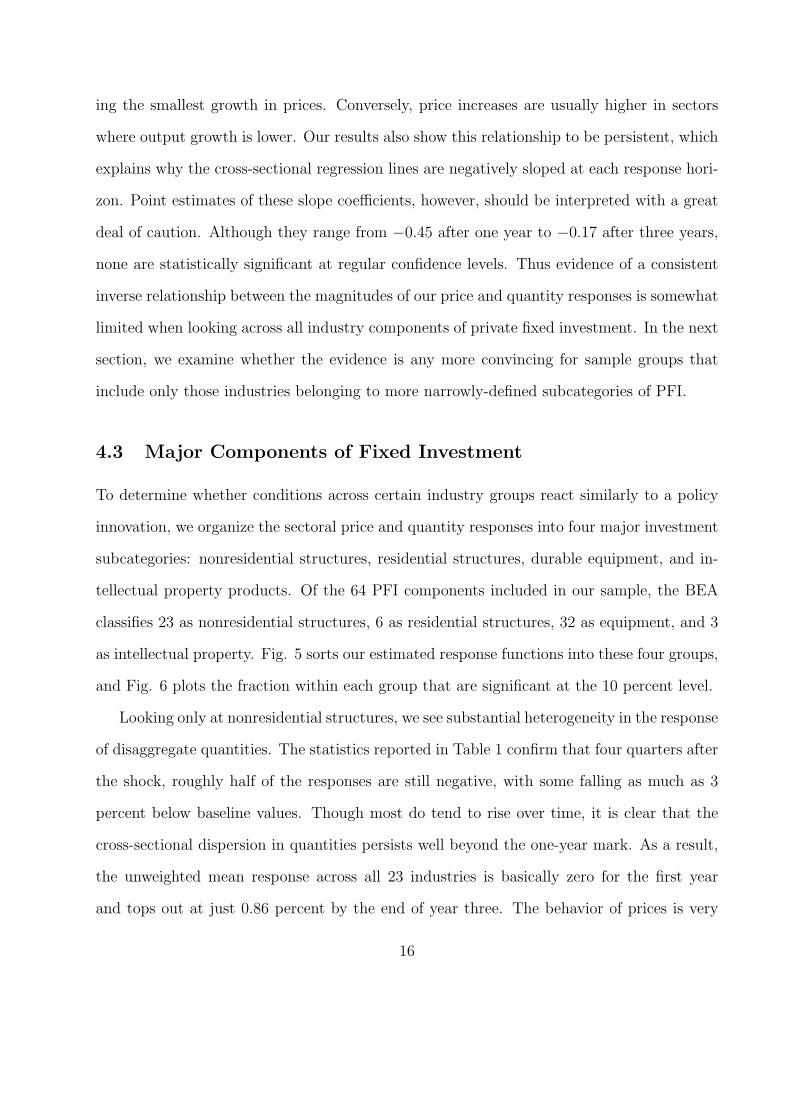
as intellectual property. Fig. 5 sorts our estimated response functions into these four groups,

and Fig. 6 plots the fraction within each group that are significant at the 10 percent level.

Looking only at nonresidential structures, we see substantial heterogeneity in the response

of disaggregate quantities. The statistics reported in Table 1 confirm that four quarters after

the shock, roughly half of the responses are still negative, with some falling as much as 3

percent below baseline values. Though most do tend to rise over time, it is clear that the

cross-sectional dispersion in quantities persists well beyond the one-year mark. As a result,

the unweighted mean response across all 23 industries is basically zero for the first year

and tops out at just 0.86 percent by the end of year three. The behavior of prices is very

16

Fig. 5. Estimated impulse responses to a one standard deviation (71 basis point) drop in the federal funds rate for all PFIquantities (left panel) and prices (right panel) are sorted by nonresidential structures, residential structures, durable equipment,and intellectual property products. Thick dashed lines are unweighted average responses across all industries within a givencategory. Thick solid lines are the responses of the aggregate quantity and price index (aggregation level 2 in Table A).

different. Excluding one industry (petroleum and natural gas wells), the distribution of prices

for nonresidential structures is more compact than the distribution for all components of PFI.

Moreover, these prices typically adjust faster and with greater intensity. The median response

eight quarters after the shock is 0.62 percent, compared to 0.19 percent when accounting for

all of PFI. Taken together, our estimates reveal that in markets for nonresidential structures,

prices are on average more responsive to monetary shocks than output.

Disparities between the adjustment of industry prices and quantities is perhaps even more

visible among producers of durable equipment. For this class of investment goods, however,

17

0 4 8 12 16

0.0

0.2

0.4

0.6

0.8

1.0

Nonresidential Structures

quarters after shock0 4 8 12 16

0.0

0.2

0.4

0.6

0.8

1.0

Residential Structures

quarters after shock

0 4 8 12 160.0

0.2

0.4

0.6

0.8

1.0Equipment

quarters after shock0 4 8 12 16

0.0

0.2

0.4

0.6

0.8

1.0Intellectual Property

quarters after shock

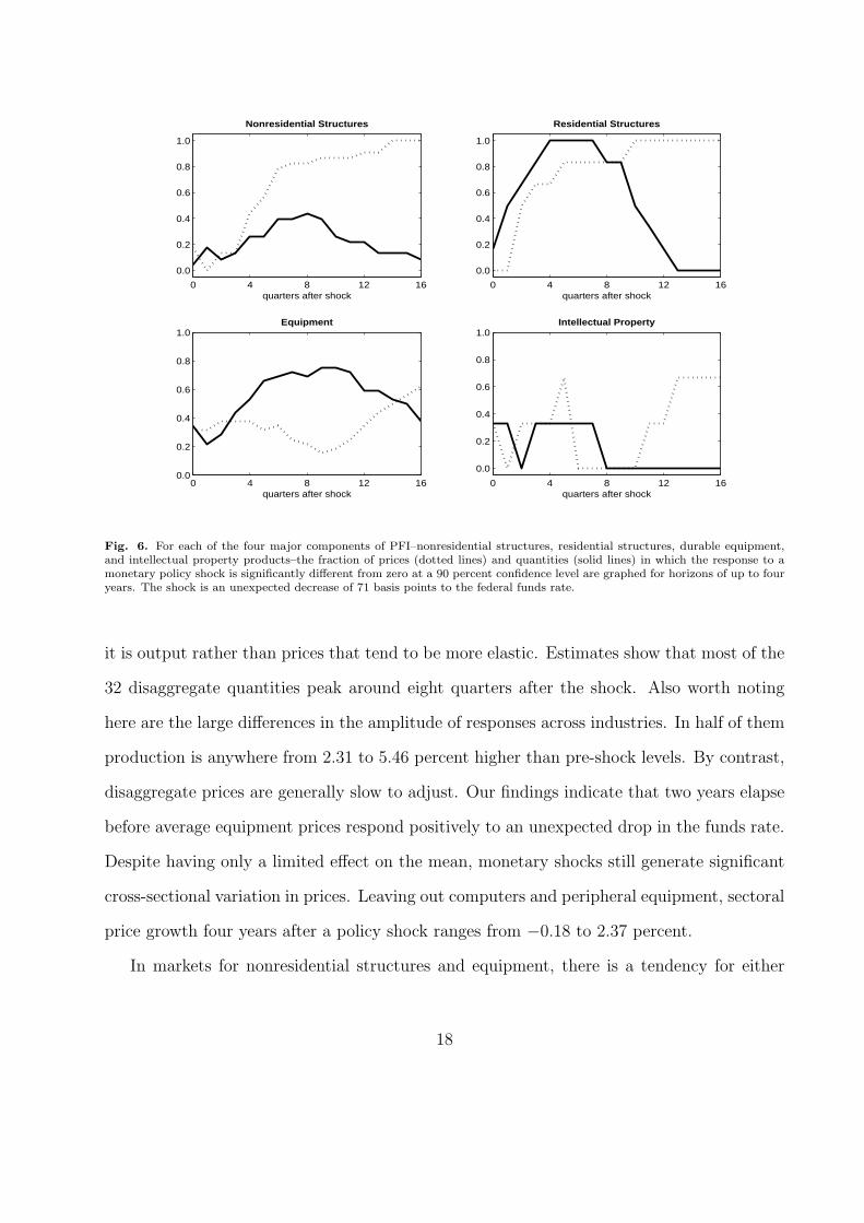
Fig. 6. For each of the four major components of PFI–nonresidential structures, residential structures, durable equipment,and intellectual property products–the fraction of prices (dotted lines) and quantities (solid lines) in which the response to amonetary policy shock is significantly different from zero at a 90 percent confidence level are graphed for horizons of up to fouryears. The shock is an unexpected decrease of 71 basis points to the federal funds rate.

it is output rather than prices that tend to be more elastic. Estimates show that most of the

32 disaggregate quantities peak around eight quarters after the shock. Also worth noting

here are the large differences in the amplitude of responses across industries. In half of them

production is anywhere from 2.31 to 5.46 percent higher than pre-shock levels. By contrast,

disaggregate prices are generally slow to adjust. Our findings indicate that two years elapse

before average equipment prices respond positively to an unexpected drop in the funds rate.

Despite having only a limited effect on the mean, monetary shocks still generate significant

cross-sectional variation in prices. Leaving out computers and peripheral equipment, sectoral

price growth four years after a policy shock ranges from −0.18 to 2.37 percent.

In markets for nonresidential structures and equipment, there is a tendency for either

18

prices or quantities to absorb most of the effects of a policy expansion. The same rela-

tionship clearly does not describe the market for residential structures. In the quarters

immediately following an unanticipated drop in the funds rate, both prices and production

of residential structures move higher. Regarding the latter, estimates reveal that sectoral

output (excluding construction of dormitories) usually peaks four to five quarters after the

shock, and according to Table 1, the median response at this horizon is 3.32 percent. The

real effects also appear to be relatively short-lived. It takes on average about three years for

most disaggregate quantities to revert to pre-shock levels. With regard to prices, evidence

suggests that all but one respond quickly to a monetary shock. The median response exceeds

0.40 percent just one year after the shock and nears one percent by the end of year two.15

With only three sectors comprising intellectual property products, we are unable to iden-

tify any pattern in the way market conditions respond to a policy innovation. For example,

real production of entertainment, literary, and artistic originals grows by almost one percent

for the first year. Production of software and research and development, on the other hand,

both decline in the months following a funds rate shock, with the former shrinking as much

as 0.54 percent. Meanwhile, the price levels observed in these sectors display significant

inertia. Response functions indicate that two years go by before average prices start rising.

4.4 Evidence on Capital Supply Elasticities

That the prices of certain capital goods are more/less responsive to monetary shocks than

investment quantities bears some resemblance to results reported in Goolsbee (1998), Has-

sett and Hubbard (1998), and Edgerton (2010). In all three papers, the authors use data

on producers’ durable equipment to determine whether tax credits aimed at stimulating

investment demand increase real production or simply materialize in the form of higher

15That prices and quantities of residential structures are sensitive to a policy innovation echoes resultsobtained by Baumeister et al. (2013) for the durables component of personal consumption expenditures.

19

capital-goods prices. Goolsbee (1998) argues that the real effects are severely limited by the

fact that short-run equipment supply curves are inelastic. His argument is based on a series

of regressions showing that for most asset types, a 10 percent investment tax credit raises

prices by more than 8 percent. By contrast, Hassett and Hubbard (1998) and Edgerton

(2010) present regression coefficients that point to much higher capital supply elasticities.

They conclude that policy incentives designed to boost investment demand will likely have

significant effects on fixed-capital formation with only modest effects on prices.16

Since we are examining how the price and quantity of fixed investment reacts to mone-

tary rather than fiscal stimuli, our estimates can neither confirm nor discredit the findings

described above. Given the demand-side nature of the two policies, however, it may be use-

ful to draw some comparisons between the elasticities reported in this literature and those

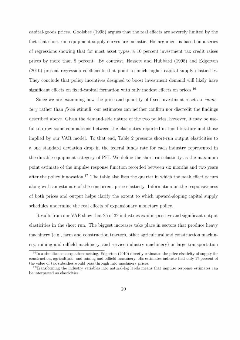
implied by our VAR model. To that end, Table 2 presents short-run output elasticities to

a one standard deviation drop in the federal funds rate for each industry represented in

the durable equipment category of PFI. We define the short-run elasticity as the maximum

point estimate of the impulse response function recorded between six months and two years

after the policy innovation.17 The table also lists the quarter in which the peak effect occurs

along with an estimate of the concurrent price elasticity. Information on the responsiveness

of both prices and output helps clarify the extent to which upward-sloping capital supply

schedules undermine the real effects of expansionary monetary policy.

Results from our VAR show that 25 of 32 industries exhibit positive and significant output

elasticities in the short run. The biggest increases take place in sectors that produce heavy

machinery (e.g., farm and construction tractors, other agricultural and construction machin-

ery, mining and oilfield machinery, and service industry machinery) or large transportation

16In a simultaneous equations setting, Edgerton (2010) directly estimates the price elasticity of supply forconstruction, agricultural, and mining and oilfield machinery. His estimates indicate that only 17 percent ofthe value of tax subsidies would pass through into machinery prices.

17Transforming the industry variables into natural-log levels means that impulse response estimates canbe interpreted as elasticities.

20

Table 2

Output and price elasticities for durable equipment

Output Price

Industry elasticity Period elasticity

Computers and peripheral equipment 2.814 [0.51, 5.37] 8 −2.431 [−3.73,−1.35]

Communication equipment 1.809 [0.60, 3.14] 8 −0.450 [−0.88,−0.06]

Electro-medical equipment 2.788 [1.01, 4.79] 6 −0.492 [−1.02,−0.11]

Medical instruments 0.391 [−0.31, 1.07] 3 −0.128 [−0.29, 0.03]

Nonmedical instruments 1.460 [0.54, 2.38] 8 −0.209 [−0.42,−0.01]

Photocopy & related equipment 0.882 [−1.83, 3.69] 6 −0.493 [−1.09, 0.04]

Office & accounting equipment 4.639 [2.25, 7.32] 8 −0.263 [−0.53,−0.01]

Fabricated metal products 0.844 [−0.30, 2.00] 8 0.398 [−0.03, 0.86]

Steam engines −0.153 [−3.30, 3.03] 2 −0.122 [−0.47, 0.23]

Internal combustion engines 3.303 [2.12, 4.62] 8 −0.034 [−0.43, 0.34]

Metalworking machinery 1.654 [−0.11, 3.29] 8 0.064 [−0.30, 0.43]

Special industry machinery, n.e.c. 0.824 [−0.25, 1.92] 7 −0.010 [−0.39, 0.36]

General industrial & materials handling 2.179 [1.17, 3.21] 8 −0.046 [−0.34, 0.25]

Electrical transmission & distribution apparatus 1.553 [0.71, 2.41] 8 −0.254 [−0.61, 0.07]

Trucks, buses, & truck trailers 4.212 [2.50, 6.03] 6 −0.071 [−0.35, 0.20]

Autos 1.807 [0.70, 2.99] 5 −0.038 [−0.44, 0.35]

Aircraft 1.895 [−0.98, 4.99] 8 0.258 [−0.03, 0.56]

Ships & boats 4.511 [1.85, 7.38] 8 0.198 [−0.06, 0.44]

Railroad equipment 3.443 [0.42, 6.75] 8 0.625 [0.06, 1.19]

Household furniture 1.657 [0.07, 3.28] 6 −0.059 [−0.26, 0.14]

Other furniture 1.600 [0.65, 2.60] 6 −0.055 [−0.35, 0.21]

Farm tractors 4.614 [2.66, 6.62] 5 −0.397 [−0.68,−0.12]

Other agricultural machinery 2.604 [1.08, 4.19] 8 −0.045 [−0.37, 0.26]

Construction tractors 5.932 [2.76, 9.20] 6 −0.040 [−0.43, 0.33]

Other construction machinery 4.383 [2.41, 6.43] 7 0.079 [−0.29, 0.44]

Mining & oilfield machinery 3.842 [0.02, 7.97] 8 0.175 [−0.40, 0.74]

Service industry machinery 1.560 [0.72, 2.46] 7 −0.188 [−0.42, 0.01]

Household appliances 3.432 [1.97, 4.99] 6 −0.302 [−0.59,−0.03]

Miscellaneous electrical 3.562 [1.94, 5.37] 8 −0.024 [−0.31, 0.25]

Other 2.447 [1.58, 3.42] 8 −0.362 [−0.69,−0.07]

Less: Sale of equipment scrap, excluding autos 5.461 [3.09, 8.06] 8 2.034 [0.00, 4.07]

Residential equipment 1.772 [0.99, 2.64] 6 −0.306 [−0.50,−0.12]

Notes: The table reports output and price elasticities to a 71 basis point drop in the federal funds rate for each industry in thedurable equipment category of PFI (ordered as they appear in Table A). Output elasticity is the maximum point estimate ofthe sectoral response function recorded between six months and two years after the funds rate shock. Period is the number ofquarters after the shock in which the peak effect occurs. Price elasticity is the estimate of the sectoral price response functionthat prevails during the quarter identified in the preceding column. Bracketed numbers are 90 percent confidence intervals.

21

equipment (e.g., trucks, buses, and truck trailers, autos, ships and boats, and railroad equip-

ment). A negative funds rate innovation boosts real production in these industries anywhere

from 1.5 to 6 percent within two years. Yet over the same period, just 8 of 32 industries sus-

tain higher prices, and in only two cases is the increase statistically above zero at a 90 percent

confidence level. According to our estimates, a larger share actually experience a significant

decline in prices. For example, sectors that produce information processing equipment (e.g.,

computers, communication, and electro-medical equipment, nonmedical instruments, and

office and accounting equipment) see prices falling between 0.2 and 2.5 percent.18

The evidence in Table 2 tells a consistent story about markets for durable equipment.

Monetary expansions, which increase the demand for fixed investment, lead to significant

growth in real quantities with few discernible price increases.19 These findings are clearly at

odds with the notion put forth by Goolsbee (1998) that equipment supply curves are inelastic

in the short run. Instead, they favor the opposite interpretation of the data suggested by

Hassett and Hubbard (1998) and Edgerton (2010) that capital supply elasticities are quite

large. Under such conditions, the effects of a stimulative demand shock would show up in

quantities rather than prices.

While not part of Goolsbee’s original analysis, disaggregated data on nonresidential struc-

tures is actually more consistent with the view that capital supply curves are relatively

inelastic in the short run. Table 3 presents output and price elasticities for each indus-

try comprising the nonresidential structures component of PFI. In sharp contrast to the

equipment category, our estimates show a positive and significant price elasticity in 15 of

23 industries. We observe some of the biggest price increases, ranging from 0.6 to 2.1 per-

cent, among producers of petroleum and natural gas wells as well as commercial and health

18These negative price elasticities may be partly attributable to difficulties in correcting the investmentdeflators for unmeasured quality improvements. See Goolsbee (1998) for a discussion.

19In the traditional cost of capital model of Hall and Jorgenson (1967), demand for capital services growsuntil the rental price equals the user cost of capital, which is increasing in the interest rate. By reducinginterest rates, a monetary expansion should lower user costs and thereby raise the demand for capital services.

22

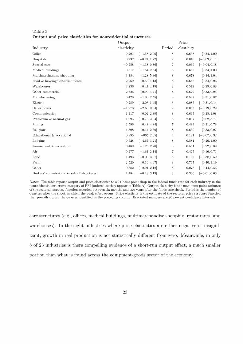
Table 3

Output and price elasticities for nonresidential structures

Output Price

Industry elasticity Period elasticity

Office 0.291 [−1.58, 2.06] 8 0.658 [0.34, 1.00]

Hospitals 0.232 [−0.74, 1.22] 2 0.016 [−0.09, 0.11]

Special care −0.258 [−1.38, 0.86] 2 0.069 [−0.04, 0.18]

Medical buildings 0.517 [−1.54, 2.54] 8 0.662 [0.34, 1.00]

Multimerchandise shopping 3.184 [1.28, 5.36] 8 0.678 [0.34, 1.04]

Food & beverage establishments 2.269 [0.55, 4.13] 8 0.646 [0.34, 0.96]

Warehouses 2.236 [0.41, 4.19] 8 0.572 [0.29, 0.88]

Other commercial 2.626 [0.99, 4.41] 8 0.629 [0.33, 0.94]

Manufacturing 0.429 [−1.80, 2.55] 8 0.582 [0.31, 0.87]

Electric −0.289 [−2.03, 1.45] 3 −0.085 [−0.31, 0.14]

Other power −1.278 [−2.60, 0.04] 2 0.053 [−0.19, 0.29]

Communication 1.417 [0.02, 2.89] 8 0.667 [0.25, 1.08]

Petroleum & natural gas 1.095 [−0.78, 3.04] 8 2.097 [0.62, 3.71]

Mining 2.596 [0.48, 4.84] 7 0.484 [0.21, 0.78]

Religious 1.398 [0.14, 2.69] 8 0.630 [0.33, 0.97]

Educational & vocational 0.995 [−065, 2.65] 4 0.121 [−0.07, 0.32]

Lodging −0.528 [−4.67, 3.21] 8 0.581 [0.20, 1.00]

Amusement & recreation 0.489 [−1.25, 2.20] 8 0.551 [0.22, 0.89]

Air 0.277 [−1.61, 2.14] 7 0.427 [0.16, 0.71]

Land 1.493 [−0.03, 3.07] 6 0.105 [−0.38, 0.59]

Farm 2.520 [0.16, 4.97] 8 0.767 [0.40, 1.19]

Other −0.382 [−2.91, 2.12] 8 0.078 [−0.44, 0.56]

Brokers’ commissions on sale of structures 1.484 [−0.18, 3.19] 8 0.300 [−0.01, 0.63]

Notes: The table reports output and price elasticities to a 71 basis point drop in the federal funds rate for each industry in thenonresidential structures category of PFI (ordered as they appear in Table A). Output elasticity is the maximum point estimateof the sectoral response function recorded between six months and two years after the funds rate shock. Period is the number ofquarters after the shock in which the peak effect occurs. Price elasticity is the estimate of the sectoral price response functionthat prevails during the quarter identified in the preceding column. Bracketed numbers are 90 percent confidence intervals.

care structures (e.g., offices, medical buildings, multimerchandise shopping, restaurants, and

warehouses). In the eight industries where price elasticities are either negative or insignif-

icant, growth in real production is not statistically different from zero. Meanwhile, in only

8 of 23 industries is there compelling evidence of a short-run output effect, a much smaller

portion than what is found across the equipment-goods sector of the economy.

23

5 Concluding Remarks

We employ disaggregate data spanning all industry categories of private fixed investment to

examine how capital-goods prices and real investment quantities respond to an aggregate

monetary shock. Examining the full spectrum of industries together reveals that while most,

but not all, experience growth in real output, there is considerable heterogeneity in the

timing and magnitude of the effects. Moreover, the dispersion in quantities is accompanied

by broad cross-sectional variation in the response of investment prices. One interpretation

of this finding is that monetary nonneutralities are pervasive in markets for fixed capital.

In addition to distributional effects, the data exposes certain patterns in the way market

conditions within more narrowly-defined asset classes react to a policy disturbance. Across

markets for durable equipment, output responses tend to be elastic while price responses

tend to be sluggish. Among producers of nonresidential structures, it is prices rather than

quantities that are frequently more responsive. Suppliers of residential structures see both

variables respond swiftly to a policy shock. These findings along with others documented in

the paper contribute to recent efforts that shed light on the monetary transmission mech-

anism using information drawn from sectoral price and output data. That we find strong

evidence of heterogeneity in the response functions speaks to the importance of understand-

ing the behavior of capital-goods prices and fixed investment at the disaggregate level.

24

References

Altissimo, Filippo; Mojon, Benoit and Zaffaroni, Paolo. “Can Aggregation Explainthe Persistence of Inflation?” Journal of Monetary Economics, March 2009, 56(2), pp.231-41.

Balke, Nathan S. and Wynne, Mark A. “The Relative Price Effects of MonetaryShocks.” Journal of Macroeconomics, March 2007, 29(1), pp. 19-36.

Barsky, Robert B.; House, Christopher L. and Kimball, Miles S. “Sticky-PriceModels and Durable Goods.” The American Economic Review, June 2007, 97(3), pp.984-98.

Barth, Marvin J. III and Ramey, Valerie A. “The Cost Channel of Monetary Trans-mission.” NBER Macroeconomics Annual 2001, January 2002, 16, pp. 199-240.

Baumeister, Christiane; Liu, Philip and Mumtaz, Haroon. “Changes in the Effectsof Monetary Policy on Disaggregate Price Dynamics.” Journal of Economic Dynamics

and Control, March 2013, 37(3), pp. 543-60.

Bernanke, Ben S. and Blinder, Alan S. “The Federal Funds Rate and the Channels ofMonetary Transmission.” The American Economic Review, September 1992, 82(4), pp.901-21.

Bernanke, Ben S. and Gertler, Mark. “Inside the Black Box: The Credit Channel ofMonetary Policy Transmission.” Journal of Economic Perspectives, Fall 1995, 9(4), pp.27-48.

Bils, Mark; Klenow, Peter J. and Kryvtsov, Oleksiy. “Sticky Prices and MonetaryPolicy Shocks.” Quarterly Review, Federal Reserve Bank of Minneapolis, Winter 2003,27(1), pp. 2-9.

Boivin, Jean; Giannoni, Marc P. and Mihov, Ilian. “Sticky Prices and MonetaryPolicy: Evidence from Disaggregated US Data.” The American Economic Review, March2009, 99(1), pp. 350-84.

Carlino, Gerald and DeFina, Robert. “The Differential Regional Effects of MonetaryPolicy.” The Review of Economics and Statistics, November 1998, 80(4), pp. 572-87.

Christiano, Lawrence J.; Eichenbaum, Martin and Evans, Charles L. “MonetaryPolicy Shocks: What Have We Learned and to What End?” in John B. Taylor and MichaelWoodford, eds., Handbook of Macroeconomics, 1(A), North-Holland, Amsterdam, 1999,pp. 65-148.

25

Clark, Todd E. “Disaggregate Evidence on the Persistence of Consumer Price Inflation.”Journal of Applied Econometrics, July/August 2006, 21(5), pp. 563-87.

Davis, Steven J. and Haltiwanger, John H. “Sectoral Job Creation and DestructionResponses to Oil Price Changes.” Journal of Monetary Economics, December 2001, 48(3),pp. 465-512.

Dedola, Luca and Lippi, Francesco. “The Monetary Transmission Mechanism: Evidencefrom the Industries of Five OECD Countries.” European Economic Review, August 2005,49(6), pp. 1543-69.

Edgerton, Jesse. “Estimating Machinery Supply Elasticities Using Output Price Booms.”Federal Reserve Board Finance and Economics Discussion Series, December 2010.

Enders, Walter and Ma, Jun. “Sources of the Great Moderation: A Time-Series Analysisof GDP Subsectors.” Journal of Economic Dynamics and Control, January 2011, 35(1),pp. 67-79.

Erceg, Christopher and Levin, Andrew. “Optimal Monetary Policy with Durable Con-sumption Goods.” Journal of Monetary Economics, October 2006, 53(7), pp. 1341-59.

Goolsbee, Austan. “Investment Tax Incentives, Prices, and the Supply of Capital Goods.”The Quarterly Journal of Economics, February 1998, 113(1), pp. 121-48.

Hall, Robert E. and Jorgenson, Dale W. “Tax Policy and Investment Behavior.” The

American Economic Review, June 1967, 57(3), pp. 391-414.

Hassett, Kevin A. and Hubbard, Glenn R. “Are Investment Incentives Blunted byChanges in Prices of Capital Goods?” International Finance, October 1998, 1(1), pp.103-25.

Lastrapes, William D. “Estimating and Identifying Vector Autoregressions Under Diag-onality and Block Exogeneity Restrictions.” Economics Letters, April 2005, 87(1), pp.75-81.

. “Inflation and the Distribution of Relative Prices: The Role of Productivity andMoney Supply Shocks.” Journal of Money, Credit and Banking, December 2006, 38(8),pp. 2159-98.

Leeper, Eric M.; Sims, Christopher A. and Zha, Tao. “What Does Monetary PolicyDo?” Brookings Papers on Economic Activity, 1996, 27(2), pp. 1-78.

Loo, Clifton Mark and Lastrapes, William D. “Identifying the Effects of Money SupplyShocks on Industry-Level Output.” Journal of Macroeconomics, Summer 1998, 20(3), pp.431-49.

Sims, Christopher A. “Interpreting the Macroeconomic Time Series Facts: The Effects ofMonetary Policy.” European Economic Review, June 1992, 36(5), pp. 975-1000.

26

Appendix

Table A

Components of private fixed investment in 2007

Aggregation level

Component 1 2 3 4 5 6

1. Nonresidential 73.614

2. Structures 19.049

3. Commercial & health care 6.967

4. Office1 2.371 2.371 2.371

5. Health care 1.535

6. Hospitals & special care 1.191

7. Hospitals 1.058

8. Special care 0.133

9. Medical buildings 0.344 0.344

10. Multimerchandise shopping 1.332 1.332 1.332

11. Food & beverage establishments 0.308 0.308 0.308

12. Warehouses 0.648 0.648 0.648

13. Other commercial2 0.773 0.773 0.773

14. Manufacturing 1.542 1.542 1.542 1.542

15. Power & communication 3.129

16. Power 2.075

17. Electric 1.590 1.590

18. Other power 0.485 0.485

19. Communication 1.054 1.054 1.054

20. Mining exploration, shafts, & wells 3.918

21. Petroleum & natural gas 3.636 3.636 3.636

22. Mining 0.282 0.282 0.282

23. Other structures 3.493

24. Religious 0.288 0.288 0.288

25. Educational & vocational 0.657 0.657 0.657

26. Lodging 1.304 1.304 1.304

27. Amusement & recreation 0.469 0.469 0.469

28. Transportation 0.345

29. Air 0.038 0.038

30. Land3 0.307 0.307

31. Farm 0.241 0.241 0.241

32. Other4 0.170 0.170 0.170

33. Brokers’ commissions on sale of structures 0.130 0.130 0.130

34. Net purchases of used structures −0.112 −0.112 −0.112

35. Equipment 33.948

36. Information processing equipment 11.623

37. Computers and peripheral equipment 3.362 3.362 3.362

38. Communication equipment 4.069 4.069 4.069

39. Medical equipment & instruments 2.772

40. Electro-medical equipment 1.396 1.396

41. Medical instruments 1.376 1.376

42. Nonmedical instruments 0.999 0.999 0.999

43. Photocopy & related equipment 0.251 0.251 0.251

44. Office & accounting equipment 0.169 0.169 0.169

Notes: The table reports nominal spending on each component as a percentage share of total private fixed investment (PFI) in2007. Shares are listed for every level of aggregation in the underlying NIPA series. The highest aggregation level (1 ) has onlytwo components while the lowest (6 ) breaks PFI into 67 components. At each level, the disaggregate shares sum to 100.

27

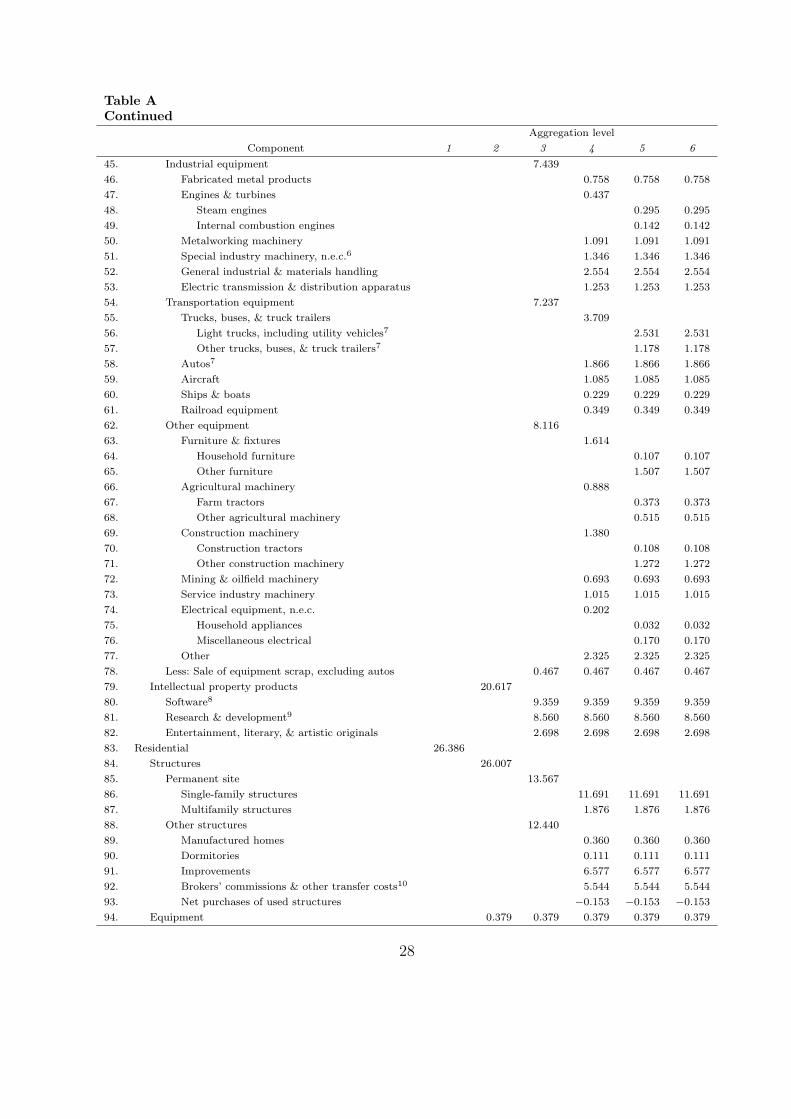
Table A

Continued

Aggregation level

Component 1 2 3 4 5 6

45. Industrial equipment 7.439

46. Fabricated metal products 0.758 0.758 0.758

47. Engines & turbines 0.437

48. Steam engines 0.295 0.295

49. Internal combustion engines 0.142 0.142

50. Metalworking machinery 1.091 1.091 1.091

51. Special industry machinery, n.e.c.6 1.346 1.346 1.346

52. General industrial & materials handling 2.554 2.554 2.554

53. Electric transmission & distribution apparatus 1.253 1.253 1.253

54. Transportation equipment 7.237

55. Trucks, buses, & truck trailers 3.709

56. Light trucks, including utility vehicles7 2.531 2.531

57. Other trucks, buses, & truck trailers7 1.178 1.178

58. Autos7 1.866 1.866 1.866

59. Aircraft 1.085 1.085 1.085

60. Ships & boats 0.229 0.229 0.229

61. Railroad equipment 0.349 0.349 0.349

62. Other equipment 8.116

63. Furniture & fixtures 1.614

64. Household furniture 0.107 0.107

65. Other furniture 1.507 1.507

66. Agricultural machinery 0.888

67. Farm tractors 0.373 0.373

68. Other agricultural machinery 0.515 0.515

69. Construction machinery 1.380

70. Construction tractors 0.108 0.108

71. Other construction machinery 1.272 1.272

72. Mining & oilfield machinery 0.693 0.693 0.693

73. Service industry machinery 1.015 1.015 1.015

74. Electrical equipment, n.e.c. 0.202

75. Household appliances 0.032 0.032

76. Miscellaneous electrical 0.170 0.170

77. Other 2.325 2.325 2.325

78. Less: Sale of equipment scrap, excluding autos 0.467 0.467 0.467 0.467

79. Intellectual property products 20.617

80. Software8 9.359 9.359 9.359 9.359

81. Research & development9 8.560 8.560 8.560 8.560

82. Entertainment, literary, & artistic originals 2.698 2.698 2.698 2.698

83. Residential 26.386

84. Structures 26.007

85. Permanent site 13.567

86. Single-family structures 11.691 11.691 11.691

87. Multifamily structures 1.876 1.876 1.876

88. Other structures 12.440

89. Manufactured homes 0.360 0.360 0.360

90. Dormitories 0.111 0.111 0.111

91. Improvements 6.577 6.577 6.577

92. Brokers’ commissions & other transfer costs10 5.544 5.544 5.544

93. Net purchases of used structures −0.153 −0.153 −0.153

94. Equipment 0.379 0.379 0.379 0.379 0.379

28

Legend/Footnotes

1. Consists of office buildings, except those constructed at manufacturing sites and thoseconstructed by power utilities for their own use. Includes all financial buildings.

2. Includes buildings and structures used by the retail, wholesale and selected serviceindustries. Consists of auto dealerships, garages, service stations, drug stores, restau-rants, mobile structures, and other structures used for commercial purposes. Bus ortruck garages are included in transportation.

3. Consists primarily of railroads.

4. Includes water supply, sewage and waste disposal, public safety, highway and street,and conservation and development.

5. Consists of brokers’ commissions on the sale of residential structures and adjoiningland, title insurance, state and local documentary stamp taxes, attorney fees, titleabstract and escrow fees, and fees for surveys and engineering services.

6. n.e.c. Not elsewhere classified.

7. Includes net purchases of used vehicles

8. Excludes software “embedded,” or bundled, in computers and other equipment.

9. Research and development investment excludes expenditures for software development.Software development expenditures are included in software investment on line 80.

10. Consists of brokers’ commissions on the sale of residential structures and adjoiningland, title insurance, state and local documentary stamp taxes, attorney fees, titleabstract and escrow fees, and fees for surveys and engineering services.

29