U.U.D.M. Project Report 2011:30

Examensarbete i matematik, 15 hpHandledare och examinator: Michael MelgaardDecember 2011

Department of MathematicsUppsala University

Mountain Pass Theorems with Ekeland’s Variational Principle and an Application to the Semilinear Dirichlet Problem

Hazhar Ghaderi

MOUNTAIN PASS THEOREMS WITH EKELAND’S

VARIATIONAL PRINCIPLE AND AN APPLICATION TO THE

SEMILINEAR DIRICHLET PROBLEM.

Bachelor Thesis for The Bachelor of Science Programme in Mathematics,

15hp.

Examensjobb for Kandidatprogrammet i matematik, 15hp.

Supervisor: Michael Melgaard

HAZHAR GHADERI

Abstract. We will in this paper prove the one-dimensional mountain pass

theorem, and state the finite dimensional one of Courant. We will also give

a proof of Ekeland’s variational principle, which is then used to prove theinfinite-dimensional mountain pass theorem of Ambrosetti and Rabinowitz.

We will also discuss some applications of the MPT, in particular we will show

the existence of weak solutions of the semi-linear Dirichlet problem.

ΣAMMANFATTNING I detta papper bevisar vi Ambrosettis och Rabinowitzs

‘Mountain Pass Theorem’ (MPT), vilket vi kommer att gora med hjalp av

Ekelands variationsprincip som vi ocksa ger ett bevis for. Vidare ger vi ettbevis av en en-dimensionel MPT som visar sig vara en foljdsats av ett valkannt

elementart resultat, namligen Rolles sats. Vi diskuterar aven tillampningar av

MPT, och visar att Dirichlets semilijara problem har minst en svag losning.

Date: September, 2011.

i

ii HAZHAR GHADERI

AcknowledgementI would like to thank my supervisor Michael Melgaard.

BACHELOR THESIS iii

iv HAZHAR GHADERI

Contents

List of Figures v1. Background 12. The Finite Dimensional MPT 32.1. The One-Dimensional MPT 32.2. The N-Dimensional MPT 43. Ekeland’s Variational Principle and the MPT 93.1. Ekeland’s Variational Principle 93.2. The Mountain Pass Theorem 124. Applications 174.1. Some definitions 174.2. Nonlinear Schrodinger type equations 184.3. Existence of weak solutions to the semi linear problem. 205. Conclusion 23References 24Appendix A. Normed, Banach, Hilbert Spaces. 25A.1. Banach Spaces 25A.2. Hilbert Spaces 26Appendix B. Some Topology. 27B.1. Topological Spaces 27Appendix C. Manifolds and The Heine-Borel Theorem 29C.1. A compactness theorem and manifolds 29

BACHELOR THESIS v

List of Figures

1 Mountainous landscape where the hue of the color is proportional to the‘height’ of the landscape, red being ‘highest’ and violet ‘lowest’. Noticeone mountain pass at ‘c’ and also notice the ‘path’ connecting x1 (theorigin in this case) with another minima x2 located at approximately(x, y) = (2, 1.4). 7

2 Top view of the same mountainous landscape of figure 1. Here also thehue of the color is proportional to the ‘height’ of the landscape, red being‘highest’ and violet ‘lowest’. At least two local minima can be seen, onenear the origin (x1 of theorem 2.2.1) and another one x2 near the point(2, 1.4). 8

3 The graph of the function Φ(x, y) = x2 + (x + 1)3y2, of example 3.2.2which do not satisfy the (PS) condition of the MPT. The hue of the colorindicates elevation with red highest and violet lowest. The graph showsthe “local” about (0, 0) features of the function. 14

4 The graph of the function Φ(x, y) = x2 + (x+ 1)3y2, which do not satisfythe (PS) condition of the MPT. The hue of the color indicates elevationwith red highest and violet lowest. The graph shows the more “global”features of the function. 15

BACHELOR THESIS 1

1. Background

Legend has it that when the running Carthaginian queen Dido arrived to NorthAfrica, she was offered by the local chieftain as much land as could be containedby an oxhide. One can only imagine the look on the chiefs face when he found outthat the oxhide had been cut to long thin threads, joined by the ends and laid onthe ground in the form of a circular arc which in combination with the shore linewas the desired land. Following intuition, queen Dido had chosen a circular arcto maximize the gain. Some 2700 years later, J. Steiner gave several proofs of thestatement that if there exist a figure Γ whose area is never less than that of anyother figure of the same perimeter, then Γ is a circle [11, ch. 35].

But as was pointed out by Dirichlet: Steiners proofs actually did not establishthe existence of such a figure (solution) and of course the existence of a solution isof utmost importance, for consider the following ‘proof’ that 1 is the largest integer;suppose I is the largest integer, then if I > 1 ⇒ I 2 > I, but this contradicts theassumption that I is the largest integer hence I = 1.

Ironically Dirichlet1 himself had made a similar assumption: in his case it was inconnection with (a variant of) the theorem we now call Dirichlet’s Principle namely;given an open bounded set Ω ∈ R2 and a continuous function φ : ∂Ω → R, theboundary value problem

−∆u = 0 in Ω,

u = φ on ∂Ω(1.1)

has a smooth2 solution u such that the (Dirichlet integral) functional

Φ(u) =

∫Ω

2∑i=1

(Diφ(x))2 dx (1.2)

is minimized. Even before this C. F. Gauß and Lord Kelvin had also noticed [12]that the boundary value problem (1.1) can be reduced to the problem of minimizingthe integral (1.2) for the domain Ω and admissible functions u taking specific valueson the boundary ∂Ω of Ω. Thus the positive character of the integral (1.2) leadthese gentlemen to believe in the existence of a solution for the latter problem andhence in the existence of a solution for the boundary value problem. Now, sincethe integral (1.2) is bounded from below, the existence of an infimum (a conceptnot yet perceived in the days of Dirichlet) is guaranteed but that infimum is notnecessarily a minimum and in fact some time later Weierstraß gave an example andshowed that it is not necessarily true that a positive integral actually attains itsminimum (see for instance [11, ch. 35], [12, ch. 1] and [3]).

In the end, the principle of Dirichlet (as coined by one of his students B. Rie-mann) was rescued by D. Hilbert [19], but the moral of the story is that a theoremand proof of the existence of a solution should be given at least as much weight as tohow to find the solution. With this in mind, we state and prove in the present paperan existence theorem known as the Mountain Pass Theorem, henceforth called theMPT, which under some specific conditions demonstrates the existence of a critical

1 Not only Dirichlet, but G. Green, B. Riemann and others and even the Prince himself (C. F.

Gauß).2 u ∈ C2(Ω;R) ∩ C(Ω;R) is continuous on Ω = Ω ∪ ∂Ω.

2 HAZHAR GHADERI

point of some functional3 under investigation. We will also give a very intuitivevisual (real world) interpretation of the theorem in R3, namely that of a moun-tainous terrain and a trail between two relatively distant points (section 2.2) whichexplains the eponymous theorem in R3. This is of course in connection with a finitedimensional MPT due to R. Courant [12, ch. VI] and which we will discuss in thenext section, but we will also discuss the MPT which is the infinite dimensionalMPT due to Ambrosetti and Rabinowitz (1973) [13]. We also state and prove avery interesting result due to Ekeland [6], namely his variational principle, whichcan be used to prove other results in a ‘simple’ manner, and which is what we willuse in proving the MPT. Furthermore we will give a one-dimensional MPT whichis a very common elementary result under disguise as we will see in the followingsection. In the final section we will take a look at applications of the MPT and asan example we will deal with the semi-linear Dirichlet problem.

3 In short, a functional is a function defined on a space whose elements are functions.

BACHELOR THESIS 3

2. The Finite Dimensional MPT

In this section we will present two MPTs, starting from a one dimensional MPTwhich will help in understanding the generalization to higher dimensions. We willalso introduce a compactness condition known as the Palais-Smale condition, whichas we will see is needed for the (infinite dimensional) MPT of Ambrosetti and Ra-binowitz.

2.1. The One-Dimensional MPT. We start by stating a well known lemma,namely that of Rolle.

Lemma 2.1.1 (Rolle’s Theorem). Let f ∈ C1([x1, x2];R) with x1 and x2 ∈ R suchthat x1 6= x2. If f(x1) = f(x2), then there exist at least one x3 ∈ (x1, x2) such that

f ′(x3) = 0.

Recall that as a consequence of the Heine-Borel theorem (see appendix C), theclosed interval

[x1, x2] ∈ R is compact, (2.1)

and also since f is continuous it achieves both its maximum and minimum thereby the extreme value theorem. Now, if f is constant in [x1, x2] with f(x1) = f(x2)then of course f ′(x) ≡ 0 for all x ∈ [x1, x2]. Thus if f is not constant in [x1, x2],the extreme value theorem and the condition

f(x1) = f(x2) (2.2)

implies that at least one of the extrema of f occurs in some interior point x3 of[x1, x2], thus x3 is a critical point of f .

A consequence of Rolle’s theorem (lemma 2.1.1) is the following mountain passtheorem in R, [3, p. 48].

Theorem 2.1.1 (MPT in R). Let x1 < x3 < x2 be distinct real numbers andf ∈ C1(R;R). If

f(x3) > maxf(x1), f(x2), (2.3)

then there exists a critical point ς of f in (x1, x2) such that

f(ς) = max[x1,x2]

f = inf[a,b]∈Γ

maxx∈[a,b]

f(x) (2.4)

whereΓ = [a, b]; such that a ≤ x1 < x2 ≤ b.

Remark 2.1.1. Notice that we can write Γ in the following form:

Γ = Σ ⊂ R; Σ compact and connected with x1, x2 ∈ Σ. (2.5)

Proof. If we suppose that f(x1) ≤ f(x2) (the other way around would work equallywell), then the mean value theorem implies that

there is some point x′1 ∈ [x1, x3) such that f(x′1) = f(x2). (2.6)

If we now apply Rolle’s theorem (Lemma 2.1.1) to the smallest number x′1 satisfyingcondition (2.6) we would be guarantied the existence of a maximum4 in [x′1, x2]. Itnow follows from (2.3) that

max[x1,x2]

f ≥ max[x′1,x2]

f ≥ f(x3) > maxf(x1), f(x2)

4 Because of (2.3).

4 HAZHAR GHADERI

and since [x1, x2] ∈ Γ,max

[x1,x2]f = inf

[a,b]∈Γmaxx∈[a,b]

f(x).

2.2. The N-Dimensional MPT. Recall the compactness condition (2.1) whichwe indirectly used in the one-dimensional MPT. It should be of no surprise that acompactness condition is also required in higher dimensions; indeed if we write thehigher (finite) dimensional Γ of above as

Γ = Σ ⊂ RN ; Σ compact and connected with x1, x2 ∈ Σand notice that in higher dimensions there is no guaranty that

infΣ∈Γ

maxΣ

f := c

is a maximum hence we cannot say that c is critical. We will show an example ofthis later but first some definitions. Throughout this paper, unless stated otherwise,the derivatives Φ′,Φ′′, etc. will be the generalized derivatives of Frechet defined asfollows.

Definition 2.2.1. Suppose X and Y are Banach spaces, Ω is an open subset ofX, Φ maps Ω into Y , and a ∈ Ω. If there exists Λ ∈ B(X;Y ) (the Banach space ofall bounded linear mappings of X into Y ) such that

limx→0

‖Φ(a+ x)− Φ(a)− Λx‖‖x‖

= 0, (2.7)

then Λ is called the Frechet derivative of Φ at a, denoted by Φ′(a), or sometimesDΦ(a).

Definition 2.2.2 (Palais-Smale sequences). Let X be a Banach space and

Φ : X → Ra C1-functional. We call a sequence un ∈ X a Palais-Smale sequence (PS-sequence)onX if Φ(un) is bounded and Φ′(un)→ 0. If it happens that Φ(un)→ c for some c ∈R the PS-sequence will be called a PSc-sequence.

We can now with the help of the above definition define what is meant by thePalais-Smale condition.

Definition 2.2.3 (The Palais-Smale condition). Let Φ and X be as above (defi-nition 2.2.2), we say that Φ satisfies the Palais-Smale condition on X denoted by(PS), if every PS-sequence has a converging subsequence.

Definition 2.2.4 ((PS)c). For X, Φ and c as in definition 2.2.2, we say that Φsatisfies the (local) Palais-Smale condition at the level c denoted by (PS)c if everyPSc-sequence has a converging subsequence.

Remark 2.2.1. The condition (PS) is stronger than (PS)c in the sense that if (PS)holds, then (PS)c is satisfied for all c ∈ R, while the converse is not necessarily true.

Example 2.2.1 (A polynomial map that satisfies (PS)). Suppose Φ : Rn → R is aquadratic polynomial

Φ(x) =

n∑i,j=1

aijxixj +

n∑i=1

bixi + c (2.8)

BACHELOR THESIS 5

in x = (x1, . . . , xn) ∈ Rn, which is non-degenerate in the sense that

Φ′′(x) = (aij)1≤i,j≤n

induces an invertible linear map Rn → Rn. Then Φ satisfies (PS).

Courant proved the finite dimensional MPT [12, Ch. VI] working on the theoryof unstable minimal surfaces, using a deformation lemma and the assumption thatΦ becomes infinite at the boundary5 of the domain under consideration. Here’s amodern version (see [3, ch. 5] and [17, ch. II] for instance) of that where we insteadassume that Φ is coercive, that is, it tends to +∞ as ‖x‖ → +∞.

Theorem 2.2.1 (MPT in RN ). Suppose that Φ ∈ C1(RN ;R) is coercive and pos-sesses two seperate strict 6 relative minima x1 and x2. Then it possesses a thirdcritical point x3 which is not a relative minimizer 7 and hence distinct from x1 andx2, characterized by the minimax principle

Φ(x3) = infΣ∈Γ

maxx∈Σ

Φ(x),

whereΓ = Σ ⊂ RN ; Σ is compact and connected with x1, x2 ∈ Σ.

is the class of ‘paths’ connecting x1 and x2.

Remark 2.2.2. We will skip the proof of this theorem but mention that in theoriginal proof [12], Courant uses a deformation where points P ∈ Σ are moved intoP ′ ∈ Σ′ along the direction of gradient of Φ such that Φ(P ′) < Φ(P ), where Σand Σ′ are “minimizing connecting sets” connecting x1 to x2. For other proofs see[17, 3].

First off, one should ask wherein lies any compactness condition in the abovetheorem, for we did not mention anything regarding compactness in stating it (ex-cept in connection with Σ). Actually, as is seen in the proof of this theorem in [17],the compactness is induced by the coercivity of Φ. The following proposition alsosheds some light on this issue.

Proposition 2.2.1. Let X = RN in definition 2.2.2 and hence Φ ∈ C1(RN ;R) inthe same definition. If the function

|Φ|+ ‖Φ′‖ : RN → R is coercive, (2.9)

then Φ satisfies (PS).

Proof. This follows from the Bolzano-Weierstrass theorem which implies that anybounded Palais-Smale sequence contains a convergent subsequence. The bounded-ness of the Palais-Smale sequence follows from our assumption that |Φ| + ‖Φ′‖ :RN → R is coercive. Notice that since X is finite dimensional it is locally compact(cf. chapter one of [7]).

Corollary 2.2.1. Let X and Φ be as in proposition 2.2.1, and replace the condition(2.9) with the following:

Φ : RN → R is coercive, (2.10)

then Φ satisfies (PS).

5 For unbounded domains, the assumption is that Φ becomes infinite at infinity.6 If x 6= xk is a point in the neighborhood of xk then Φ(x) > Φ(xk) for k = 1, 2.7 That is, in every neighborhood of x3 ∃ x such that Φ(x) < Φ(x3)

6 HAZHAR GHADERI

Remark 2.2.3. Thus we see that in finite dimensions, the coercivity of Φ impliesthat Φ satisfies (PS), but in infinite dimensional spaces the coercivity of Φ resultsin bounded compactness (and not necessarily (PS) see example 2.2.2 below) andsome incompatibility (regarding Φ ∈ C1(X) for some Banach space X, cf. [17]).

Example 2.2.2 (coercivity ; (PS) (in general) in infinite dimensional spaces). Toshow that Φ can be bounded from below and coercive but still fails to satisfy (PS)in an infinite dimensional Banach space X, consider the following example ([14, p.107]). Let

g : R+ → Rdenote a smooth function such that

g(s) =

0 if s ∈ [0, 2],

s if s ≥ 3.(2.11)

Now, Φ(u) = g(‖u‖) is bounded from below and coercive but does not satisfy (PS)cfor c = 0. To see this, notice that any sequence uj ∈ X with ‖uj‖ = 1 is such thatΦ(uj) = 0 and Φ′(uj) = 0.

Not only the negative result of the above example, but we would of course alsolike to be able to apply these minimax methods not only to bounded functionalsbut to unbounded functionals as well. Then, (PS) is the proper condition to befulfilled. Now, one should ask why the Palais-Smale condition is called an compact-ness condition. Well, if we denote by Kc the set of critical points of the (energy)functional Φ, at the (energy) level c, that is

Kc = u ∈ X; Φ(u) = c and Φ′(u) = 0,then the following proposition shows that the set Kc is compact and hence why(PS)c is called an compactness condition.

Proposition 2.2.2. Suppose that Φ satisfies (PS). Then Kc is compact for anyc ∈ R.

Proof. From (PS), it follows that any sequence (um) in Kc has a convergent sub-sequence, and by the continuity of Φ and Φ′ (recall from definition 2.2.2 thatΦ ∈ C1(X)) any accumulation point of such a sequence also lies in Kc, thus Kcis compact.

Remark 2.2.4. If K is the set of all critical points of Φ in X, and the restrictionΦ|B of Φ to a set B ⊂ K is uniformly bounded, then B is relatively compact.

Interpretation of the finite dimensional MPT. If we now go back to thefinite dimensional MPT, in particular when Φ ∈ R2 and visualize Φ(x, y) to bethe elevation at a point (x, y) in a mountainous landscape. Figure 1 shows such alandscape where the point x1 (of theorem 2.2.1) is located at the origin and anotherminimum x2 located approximately at (x, y) ≈ (2.049, 1.401). What can also beseen in figure 1 is a path Σ (out of infinitely many) connecting x1 with x2, but whatis special about this path is that it passes through the mountain pass c indicatedby a cyan colored ‘blob’. This mountain pass is the highest point on the path Σand as can be seen from both figures (1 and 2) it is a saddle point of the terrain.

A top view of the terrain is given in figure 2, where just as in figure 1, the hueof the color describes the ‘height’ or the elevation of the terrain at a given point.

BACHELOR THESIS 7

Figure 1. Mountainous landscape where the hue of the color isproportional to the ‘height’ of the landscape, red being ‘highest’and violet ‘lowest’. Notice one mountain pass at ‘c’ and also noticethe ‘path’ connecting x1 (the origin in this case) with anotherminima x2 located at approximately (x, y) = (2, 1.4).

The highest points on the ‘mountains’ are colored dark red and the lowest pointsare colored violet.

Now, the Mountain Pass Theorem (theorem 2.2.1) is an existence theorem thatunder the given conditions8 guaranties the existence of the point c of figure 1. Intu-itively, the existence of c should be clear to anyone who have wandered mountainsor hills at some point.

For if we imagine two villages, village number one and village number two,

located at the deepest points, x1 and x2 respectively of two valleys surrounded

by a ring of mountains or hills. Suppose you are in village number one and you

would like to get to village number two: then unless you want to get extra tired,

you would search for a route with the least amount of rise. Naturally, such a

route passes through a mountain pass, which is not a maximum of the surrounding

landscape since by definition you searched for the route of minimal rise. Nor is it

a minimum because you just climed up out of your valley to get to the mountain

pass, hence intuitively it should be a saddle point of the local landscape. This is

of course only intuitively and lacks any kind of mathematical rigor. We will in the

following section give an example (ex. 3.2.1) where some geometric properties of

the ‘landscape’ are satisfied but without any kind of compactness condition, we

8 Actually the function whose graph is seen in figures 1 and 2 is merely of pedagogical valuein the sense that it’s not even coercive hence does not satisfy the conditions of theorem 2.2.1.

8 HAZHAR GHADERI

Figure 2. Top view of the same mountainous landscape of figure1. Here also the hue of the color is proportional to the ‘height’ ofthe landscape, red being ‘highest’ and violet ‘lowest’. At least twolocal minima can be seen, one near the origin (x1 of theorem 2.2.1)and another one x2 near the point (2, 1.4).

won’t be able to show the existence of a mountain pass critical point, such as c in

figure 1. The original proof of theorem 2.2.1 due to Courant [12] resembles this

intuitive approach, although with a compactness condition namely that Φ→∞ on

the boundary of the region (even if the boundary is +∞ cf. footnote 5) or as we

did by enforcing coercivity.

BACHELOR THESIS 9

3. Ekeland’s Variational Principle and the MPT

This section is dedicated to two celebrated results, namely: Ekeland’s variationalprinciple which we will give a thorough proof of and which we will use to prove theother result; which is the mountain pass theorem of Ambrosetti and Rabinowitz[13], which generalizes the MPT of Courant (theorem 2.2.1) to infinite dimensionalBanach spaces.

There are several ways to prove the theorem: for instance by various deformationlemmata such as in [13, 14, 5, 17, 3]; but one can also utilize a theorem due to I.Ekeland [6] known as Ekeland’s variational principle or the ε-principle. We shalluse the latter mentioned result and for that we need some definitions.

3.1. Ekeland’s Variational Principle.

Definition 3.1.1. Let X be a Banach space and Φ : X → R a functional boundedfrom below i.e.

inf Φ > −∞.

We say that the sequence (xj)j is a minimizing sequence if

limj

Φ(xj) = infx∈X

Φ(x). (3.1)

The functional Φ : X → R is said to be (weakly) lower semi-continuous if wheneverlimj xj = x strongly (weakly) it follows

lim infj→∞

Φ(xj) ≥ Φ(x). (3.2)

Moreover we say that the functional Φ : X → R is sequentially weakly continuousif whenever limj xj = x weakly, it follows

limj

Φ(xj) ≥ Φ(x). (3.3)

Consider an complete metric space X and a lower semicontinuous functionalΦ : X → R ∪ +∞, which is bounded from below. If (xj)j is a minimizing se-quence, then for every ε > 0 there exists j0 such that for j > j0

Φ(xj) ≤ infX

Φ + ε.

We call x an ε-minimum point of Φ if

Φ(x) ≤ infX

Φ + ε.

From the existence of such an ε-minimum, Ekeland found a number of other prop-erties of Φ three of which are stated in the following theorem, the proof of whichwe will give, other proofs can be found in [6, 20, 8].

10 HAZHAR GHADERI

Theorem 3.1.1 (Ekeland’s Variational Principle). Let X be a complete metricspace and Φ : X → R ∪ ∞ a lower semicontinuous functional, not identicallyequal to +∞ (Φ 6≡ +∞) which is bounded from below (inf Φ > −∞).

Let ε > 0 and x ∈ X such that

Φ(x) ≤ infu∈X

Φ(u) + ε, (x is an ε-minimum of Φ).

Then, for all δ > 0 there exists y = y(ε) ∈ X such that:

Φ(y) ≤ Φ(x), (3.4)

dist(x, y) ≤ δ, (3.5)

and

Φ(y) < Φ(u) +ε

δdist(u, y), ∀u ∈ X, such that u 6= y. (3.6)

Proof. Following [20] let us define a partial ordering in X by

u ≺ v ⇐⇒ Φ(u) ≤ Φ(v)− ε

δdist(u, v),

depending on δ. It immediately follows that the following relations hold:

u ≺ v, ∀u ∈ X,u ≺ v, v ≺ u =⇒ u = v, ∀u, v ∈ X,u ≺ v, v ≺ w =⇒ u ≺ w, ∀u, v, w ∈ X.

Too prove the last one suppose that for u, v, w ∈ X we have

u ≺ v ∧ v ≺ w,

that is

Φ(u) ≤ Φ(v)− ε

δdist(u, v),

and

Φ(v) ≤ Φ(w)− ε

δdist(v, w),

respectively. Then it’s easy to see that

Φ(u) ≤ Φ(w)− ε

δdist(u,w),

this follows from the triangle inequality (cf. appendix A)

Φ(u) ≤ Φ(v)− ε

δdist(u, v)

≤ Φ(w)− ε

δ[dist(v, w) + dist(u, v)]

≤ Φ(w)− ε

δdist(u,w).

Now, we shall define by induction a decreasing sequence of sets (Sn)n which we willshow are closed and that their intersection⋂

n

Sn,

reduces to a single point, namely y and then we check that y satisfies properties(3.4) - (3.6), to complete the proof.

BACHELOR THESIS 11

Thus let z1 = x, S1 = u ∈ X : u ≺ z1 and construct inductively a sequence(zn)n via:

z2 ∈ S1, Φ(z2) ≤ infS1

Φ +ε

22,

S2 = u ∈ X : u ≺ z2, . . .

zn+1 ∈ Sn, Φ(zn+1) ≤ infSn

Φ +ε

2n+1,

Sn = u ∈ X : u ≺ zn.Since zn+1 ∈ Sn, i.e. zn+1 ≺ zn for all n, we have that

S1 ⊃ S2 ⊃ · · · ⊃ Sn ⊃ Sn+1 ⊃ · · · .We claim that

limn→∞

diam Sn = 0. (3.7)

First let us show that the sets Sn are closed. Thus consider yj ∈ Sn with limj yj =y ∈ X, that is

Φ(yj) ≤ Φ(zn)− ε

δdist(yj , zn).

Because of the lower semicontinuity of Φ and continuity of the distance function,we get upon letting j →∞ that

Φ(y) ≤ Φ(zn)− ε

δdist(y, zn),

hence y ∈ Sn.Now, to prove (3.7), let u ∈ Sn i.e.

Φ(u) ≤ Φ(zn)− ε

δdist(u, zn).

By u ∈ Sn ⊂ Sn−1

Φ(zn) ≤ infSn−1

Φ +ε

2n≤ Φ(u) +

ε

2n

and

Φ(zn)− ε

2n≤ Φ(u) ≤ Φ(zn)− ε

δdist(u, zn),

It follows that1

δdist(u, zn) ≤ 1

2n, ∀u ∈ Sn.

Then, for any u1 and u2 ∈ Sn1

δdist(u1, u2) ≤ 1

δdist(u1, zn) +

1

δdist(u2, zn) ≤ 1

2n−1

hence

diamSn → 0 as n→∞,and since X is a complete metrics space, (Sn)n a decreasing sequence of closed setswith the property (3.7), it follows that

∞⋂n=1

Sn = y = y(ε).

All that is left is to show that this y satisfies the properties (3.4), (3.5) and (3.6).Now

y ∈ S1, and y ≺ z1 = x⇒ Φ(y) ≤ Φ(x)− ε

δdist(x, y) ≤ Φ(x),

12 HAZHAR GHADERI

hence property (3.4) holds. For the next one (3.5), we have

ε

δdist(y, x) ≤ Φ(x)− Φ(y)

≤ infu∈X

Φ(u) + ε− Φ(y)

≤ ε.

And finally to show that (3.6) holds let u 6= y. If for some u ∈ X we had u ≺ y, wewould have u ≺ zn for all n. It follows that

u ∈∞⋂n=1

Sn

hence u = y. Therefore y ≺ u i.e.

Φ(u) ≥ Φ(y) +ε

δdist(y, u)

> Φ(y)− ε

δdist(y, u),

i.e. property (3.6) is true as well and we are done.

Remark 3.1.1. As Jabri [3] points out: Ekeland’s variaitonal principle is an uncer-tainty principle in the sense that; “the closer y is to x, the larger its derivative maybe. And conversely, the smaller is its derivative, more precise is its position sinceit has to be in a larger ball of center x”.

3.2. The Mountain Pass Theorem. We have seen in the one-dimensional MPTthat there is not only a compactness condition needed (2.1) but also a geometriccondition, cf. equation (2.2). Similarly here we require not only the Palais-Smalecompactness condition but also a geometric condition which we will introduce now:but first let us define the class of all paths joining u = 0 and u = e;

Γ := γ ∈ C([0, 1];X); γ(0) = 0, γ(1) = e, (3.8)

where

e ∈ X, ‖e‖ > r > 0. (3.9)

Clearly, Γ 6= ∅ since γ(t) = te is in Γ. Then we assume that the geometric condition

infu∈S(0,ρ)

Φ(u) > maxγ(0), γ(e) (3.10)

is satisfied for all

u ∈ S(0, ρ) = u ∈ X : ‖u− 0‖ ≤ ρ. (3.11)

Notice that Φ might be unbounded from below but we only require it be boundedbelow on S(0, ρ) for some ρ > 0.

BACHELOR THESIS 13

Theorem 3.2.1 (The Mountain Pass Theorem). Let X be a Banach space and

Φ : X → R

a C1-functional satisfying the Palais-Smale condition (PS). Furthermore, supposethat ∃ e, r satisfying (3.9) and that the geometric condition (3.10) is fulfilled. Then,there exists a critical value

c ≥ infu∈S(0,ρ)

Φ(u)

of Φ characterized by

c = infγ∈Γ

maxu∈γ([0,1])

Φ(u), (3.12)

with S and Γ given by (3.11) and (3.8) respectively.

Remark 3.2.1. As we have mentioned there are several ways to prove this theorem,cf. for instance Figueiredo [8] for a much more detailed treatment of the variationalprinciple, where the MPT is also proved via it. The following proof is from [3].

Proof. If we view Γ of (3.8) as a normed space for the uniform topology generatedby the norm

‖γ‖Γ = maxt∈[0,1]

|γ(t)|, for γ ∈ Γ,

and define Ψ : Γ→ R by

Ψ(γ) = maxt∈[0,1]

Φ(γ(t)).

Then, Ψ is lower semicontinuous as the upper bound of a family of lower semicon-tinuous functions. It is also bounded from below since

c = infΓ

Ψ ≥ maxΦ(0),Φ(e),

hence we can use Ekeland’s variational principle. I.e. for every ε > 0, there existsa path γε ∈ Γ such that

Ψ(γε) ≤ c+ ε, and

Ψ(γ) ≥ Ψ(γε)− ε‖γ − γε‖Γ for all γ ∈ Γ.(3.13)

Let

M(ε) :=

t ∈ [0, 1]; Φ(γε(t)) = max

s∈[0,1]Φ(γε(s))

,

then, (3.13) implies that there exists a tε ∈M(ε) such that

‖Φ′(γε(tε))‖ ≤ ε.

The (PS)c condition with Palais-Smale sequence xn = γ1/n(t1/n) then do the jobto finish the proof.

14 HAZHAR GHADERI

Recall that at the end of section 2.2 we said that the geometric condition is notenough to guaranty the existence of a critical point c of Φ. Indeed, a compactnesscondition is needed even in finite dimensional cases as was shown by Brezis andNirenberg [21, p. 942] through the following example in R2 where the Palais-Smalecondition is not satisfied.

Example 3.2.1. Let Φ(x, y) = x2 + (1− x)3y2. Choose R in such a way that

Φ(x, y) > 0 for 0 < x2 + y2 < R2

and

Φ(x0, y0) ≤ 0 for some (x0, y0) with x20 + y2

0 > R2.

Now,

∇Φ(x, y) =[2x− 3(1− x)2y2

]ex +

[2(1− x)3y

]ey

so the only critical point of Φ(x, y) is (0, 0), where Φ = 0, but c of (3.12) is positiveand hence cannot be a critical value of Φ.

A similar example is the following where the condition (PS) is not satisfied.

Example 3.2.2. Let, Φ(x, y) = x2 + (x+ 1)3y2. We claim that Φ does not satisfythe Palais-Smale condition, and its critical point (0, 0) is the only one (i.e. unique).

Figure 3. The graph of the function Φ(x, y) = x2 + (x+ 1)3y2, ofexample 3.2.2 which do not satisfy the (PS) condition of the MPT.The hue of the color indicates elevation with red highest and violetlowest. The graph shows the “local” about (0, 0) features of thefunction.

BACHELOR THESIS 15

Proof. As we remarked above, if (PS) is satisfied then (PS)c is satisfied for all c ∈ Rand in particular for c > 0. Thus let (xj , yj)j be a sequence such that

limj

(x2j + (xj + 1)3y2

j

)= c > 0,

limj

(2xj + 3(xj + 1)2y2

j

)= 0,

limj

2 (xj + 1)3yj = 0.

Now suppose that limj(xj , yj) = (x0, y0) 6= (0, 0). Taking the limit of the above weget a contradiction

x20 + (x0 + 1)3y2

0 = c > 0,

2x0 + 3(x0 + 1)2y20 = 0,

2 (x0 + 1)3y0 = 0,

→← .

Figure 4. The graph of the function Φ(x, y) = x2 + (x + 1)3y2,which do not satisfy the (PS) condition of the MPT. The hue of thecolor indicates elevation with red highest and violet lowest. Thegraph shows the more “global” features of the function.

The function Φ(x, y) = x2 + (x+ 1)3y2 of example 3.2.2, satisfies the geometriccondition of the MPT but fails to satisfy the (PS) which we saw results in that the

16 HAZHAR GHADERI

MPT is not valid for it. From the “local” graph of the function, figure 3, we seethat Φ has a minimum at (0, 0) which is the only local minimum. The hue of thecolor indicates the “elevation” of the function. In figure 4 we see a more “global”view of the function, here too the hue of the color represents the value of Φ withred being large positive and violet being large in magnitude but negative.

Having proved the variational principle and applied it to prove the MPT, we willin the following section take a look at how and where the MPT is used in applica-tions and we will also attack the semi-linear Dirichlet boundary value problem andprove that it has non-trivial weak solutions.

BACHELOR THESIS 17

4. Applications

The mountain pass theorem have a lot of applications and is especially wellsuited to semilinear (SL) elliptic boundary value problems. For instance the fol-lowing references cover that [5, p. 482], [14, p. 123] and [17, p. 102]. Ambrosettiand Zelati have for instance used the MPT to prove the existence of solutions ofperiodic orbits of conservative systems with symmetric potential [15, p. 106]. It isinteresting to see how the mentioned authors also apply a method very similar tothe MPT in proving the existence of periodic solutions for the system

q + V ′(t, q) = 0

(where ′ denotes the gradient) in the case of singular repulsive potentials, i.e. po-tentials such that

V (x)→ +∞ as x→ 0

cf. [15, p. 51]. In the monograph [3], Jabri not only gives and proves the existenceof solutions to the semilinear problem

−∆u(x) = f(x, u(x)) in Ω,

u(x) = 0 on ∂Ω,(SL)

but also treats a problem of the Ambrosetti-Prodi type

−∆u(x) = f(x, u(x)) + g(x) in Ω,

u(x) = 0 on ∂Ω,(AP)

where Ω is a bounded smooth domain of RN . Let us also mention that the origi-nal paper by Ambrosetti and Rabinowicz [13] also includes applications to integralequations.

4.1. Some definitions. In order to discuss the applications of the MPT we needto define some concepts, starting with Sobolev spaces. They are ubiquitous inapplications.

Definition 4.1.1. Let Ω ⊂ RN be an open set and m and p positive integers with1 ≤ p ≤ ∞. We define the Sobolev spaces as follows

Wm,p(Ω) := u ∈ Lp(Ω); Dαu ∈ Lp(Ω) for 0 ≤ |α| ≤ m ,

where Dαu is the weak derivative and α = (α1, . . . , αN ) ∈ NN a multi-index.

Remark 4.1.1. It can be shown [5, p. 249] that for each m = 1, . . . and 1 ≤ p ≤ ∞,Wm,p(Ω) is a Banach space.

18 HAZHAR GHADERI

We will also mention embedding and compactly embedded hence we define,

Definition 4.1.2. For two Banach spaces X and Y we say that X is continuouslyembedded into Y and denote this by X → Y if the following two conditions aresatisfied:

X is a subspace of Y, (S)

and

every convergent sequence in X is still convergent in Y, (C)

i.e. the embedding I : X → Y , u 7→ u is continuous. X is said to be compactly

embedded into Y denoted by X→→ Y if X → Y and I is compact.

4.2. Nonlinear Schrodinger type equations. Let us show how the MPT canbe applied to Nonlinear Schrodinger (NLS) type equations. These arise, not only inquantum mechanics, but for instance also in Plasma Physics and Nonlinear Optics,cf. for instance [18, ch. 14].

Recall the Schrodinger equation for a single particle, which is a linear partialdifferential equation of the form

i~∂ψ

∂t= −~2∆ψ +Q(x)ψ,

where i is the imaginary unit, ∆ is the Laplace operator, ψ = ψ(t, x) is a complex-valued (wave) function, ~ = h/2π ≈ 1.055 × 10−34 [J · s] is the (reduced) Planckconstant and (t, x) ∈ R × Rn. For many-particle (Bosonic) systems one have tointroduce nonlinear terms in order to model the mutual interaction between theparticles. To do this we expand in an odd power series

a0ψ + a1|ψ|p−1ψ + · · · , for p ≥ 3

and keep only the first nonlinear term to arrive at the NLS

i~∂ψ

∂t= −~2∆ψ + [a0 +Q(x)]ψ + a1|ψ|p−1ψ. (4.1)

Writing an ansatz for the solution to (4.1) in the form of an phase-factor and anamplitude

ψ(t, x) = eiαt/~ u(x), u(x) ∈ R 6≤0,

and plugging this into (4.1), we get an equation equivalent to (4.1) in terms of u > 0

−~2∆u+ [α+ a0 +Q(x)]u = up. (4.2)

Finally defining ~ := ε and [α+ a0 +Q(x)] := V (x) and noticing that to obtainbound state solutions (i.e. solutions with finite energy) it is natural to assume or

BACHELOR THESIS 19

enforce the condition: that the solutions u live in the Sobolev spaceW 1,2(Rn), hence−ε2∆u+ V (x)u = up,

u ∈W 1,2(Rn), u > 0.(4.3)

Using the transformation x→ εx+ x0, where x0 ∈ Rn, (4.3) is written as−∆u+ V (x+ x0)u = up,

u ∈W 1,2(Rn), u > 0,(4.4)

the solutions of which are critical points u > 0 of a functional of the form

Iε(u) = I0(u) + Iperturbed.

In particular, the unperturbed equation I ′0(u) = 0 becomes the autonomous−∆u+ V (x0)u = up,

u ∈W 1,2(Rn), u > 0,(4.5)

which resembles the radial NLS (eq. (10.2) of [16])−∆u+ V (ε|x|)u = up, in Rn

u ∈W 1,2r (Rn), u > 0.

(4.6)

Here W 1,2r (Rn) denotes the space of radial functions in W 1,2(Rn). Now, since the

embedding of W 1,2r (Rn) into Lq(Rn) is compact whenerver 2 < q < 2∗ (Rellich-

Kondrachov theorem [5, p. 272]), it is possible to show that (PS)c is satisfied andthat the mountain pass geometric condition(s) are satisfied provided that 1 < p <2∗−1 = (n+2)/(n−2). Thus we can claim that there exist a solution uε ∈W 1,2

r (Rn)of (4.6), and it is shown in [16] that for stationary x0 this solution has the form

uε(x) ∼ U0

(x− x0

ε

), 0 < U0, and ε 6= 0 small

i.e. a ‘spike’ concentrated at x0. see for instance [22] for a proper and extensivederivation. The physical interpretation is that the ‘energy’ of the particle is localizedin packets, and are not dispersive.

20 HAZHAR GHADERI

4.3. Existence of weak solutions to the semi linear problem. Let us considerthe semilinear elliptic Dirichlet problem (SL) mentioned above which is a primeexample of the applications of the MPT and is treated in many of the references,we follow [5] here:

−∆u = f(u) in Ω,

u = 0 on ∂Ω,(4.7)

where Ω is a bounded smooth domain of RN , together with the assumptions;

f smooth , (4.8a)

|f(z)| ≤ C(1 + |z|p), |f ′(z)| ≤ C(1 + |z|p−1), (4.8b)

0 ≤ F (z) ≤ σf(z)z, σ constant < 1/2, (4.8c)

a|z|p+1 ≤ |F (z)| ≤ A|z|p+1, z ∈ R, (4.8d)

where C is a constant, z ∈ R, 1 < p < (n+ 2)/(n− 2), 0 < a ≤ A, and F (z) definedas:

F (z) :=

∫ z

0

f(s) ds.

We want to show that this problem has at least one (weak) solution, to do thatone can equivalently consider the critical points of the energy functional associatedwith it, namely:

Φ[u] :=

∫Ω

1

2|Du|2 − F (u) dx, (4.9)

for u ∈ W 1,20 (Ω) := H1

0 (Ω) and whose critical points are weak solutions of (4.7).Thus, we have recast the problem into one we can try to attack via the MPT. Tothis end, we shall use the Mountain Pass Theorem restated for convenience in thefollowing compact equivalent form:

Theorem 4.3.1 (The MPT). Assume Φ ∈ C satisfies the Palais-Smale conditionand the following ones too;

Φ[0] = 0, (4.10a)

∃r, a > 0 such that Φ[u] ≥ a if ‖u‖ = r, (4.10b)

∃v ∈ H with ‖v‖ > r, Φ[v] ≤ 0. (4.10c)

Then for Γ := γ ∈ C([0, 1];H); γ(0) = 0, γ(1) = v,

c = infγ∈Γ

max0≤t≤1

Φ[γ(t)] (4.11)

is a critical value of Φ.

It’s easy to see from (4.8) that u ≡ 0 is a solution of (4.7) so we suppose u 6≡ 0and let H = H1

0 (Ω) with norm

‖u‖ =

(∫Ω

|Du|2 dx

)1/2

,

and inner product

(u, v) =

∫Ω

Du ·Dv dx,

BACHELOR THESIS 21

we can then write the energy functional as

Φ[u] :=1

2‖u‖2 −

∫Ω

F (u) dx := Φ1[u]− Φ2[u]. (4.12)

Now in order to prove the existense of a solution we need to check that Φ satisfiesthe conditions of the MPT: first let us see that Φ indeed belongs to C; for eachu, ω ∈ H we have that9

Φ1[ω] =1

2‖ω‖2 =

1

2‖u+ ω − u‖2 =

1

2‖u‖2 + (u, ω − u) +

1

2‖ω − u‖2,

so that Φ′1[u] = u hence Φ1 ∈ C. To show that Φ2 is in C needs a little more effort,one can then make use of the Lax-Milgram Theorem i.e. that for each v∗ in thedual space10 H−1(Ω) the following problem

−∆v = v∗ in Ω,

v = 0 on ∂Ω,

has a unique solution v ∈ H10 (Ω). Writing v = Kv∗ with

K : H−1(Ω)→ H10 (Ω) an isometry,

one can show (cf. [5, p. 483]) that if u ∈ H10 (Ω), then Φ′2[u] = K[f(u)] and

moreover that Φ′2 : H10 (Ω)→ H1

0 (Ω) is Lipshitz continuous on bounded sets henceΦ2 ∈ C. What’s more, we can use this to show that Φ satisfies the Palais-Smalecondition; for suppose that uk∞k=1 ⊂ H1

0 (Ω) such that

Φ[uk]∞k=1 is bounded (4.13)

and

Φ′[uk] −→ 0 in H10 (Ω), (4.14)

then from the above it follows that

uk −K(f(uk)) −→ 0 in H10 (Ω), (4.15)

hence for k sufficiently large and each ε > 0

|(Φ′[uk], v)| =∣∣∣∣∫

Ω

Duk ·Dv − f(uk)v dx

∣∣∣∣ ≤ ε‖v‖, for v ∈ H10 (Ω).

In particular letting ε = 1 and v = uk we get∫Ω

f(uk)uk dx ≤ ‖uk‖2 + ‖uk‖, (4.16)

and (4.13) implies for some constant C and all k that

1

2‖uk‖2 −

∫Ω

F (uk) dx ≤ C <∞,

thus using (4.16) and the fact that

0 ≤ F (z) ≤ σf(z)z, σ constant < 1/2,

9 One can define differentiability as follows: Φ is differentiable at u ∈ H if there exists v ∈ Hsuch that

Φ[ω] = Φ[u] + (v, ω − u) + o(‖ω − u‖), (ω ∈ H).

If v exists, it’s unique and we write Φ′[u] = v10 H−1(Ω) is the dual space to H1

0 (Ω), i.e. Φ ∈ H−1(Ω) provided Φ is a bounded linear

functional on H10 (Ω).

22 HAZHAR GHADERI

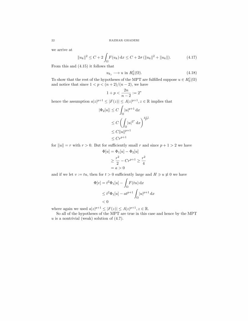
we arrive at

‖uk‖2 ≤ C + 2

∫Ω

F (uk) dx ≤ C + 2σ (‖uk‖2 + ‖uk‖). (4.17)

From this and (4.15) it follows that

ukj −→ u in H10 (Ω). (4.18)

To show that the rest of the hypotheses of the MPT are fulfilled suppose u ∈ H10 (Ω)

and notice that since 1 < p < (n+ 2)/(n− 2), we have

1 + p <2n

n− 2:= 2∗

hence the assumption a|z|p+1 ≤ |F (z)| ≤ A|z|p+1, z ∈ R implies that

|Φ2[u]| ≤ C∫

Ω

|u|p+1 dx

≤ C(∫

Ω

|u|2∗

dx

) p+12∗

≤ C‖u‖p+1

≤ Crp+1

for ‖u‖ = r with r > 0. But for sufficiently small r and since p+ 1 > 2 we have

Φ[u] = Φ1[u]− Φ2[u]

≥ r2

2− Crp+1 ≥ r2

4= a > 0

and if we let v := tu, then for t > 0 sufficiently large and H 3 u 6≡ 0 we have

Φ[v] = t2Φ1[u]−∫

Ω

F (tu) dx

≤ t2Φ1[u]− atp+1

∫Ω

|u|p+1 dx

< 0

where again we used a|z|p+1 ≤ |F (z)| ≤ A|z|p+1, z ∈ R.So all of the hypotheses of the MPT are true in this case and hence by the MPT

u is a nontrivial (weak) solution of (4.7).

BACHELOR THESIS 23

5. Conclusion

We now know why existence theorems such as the MPT are important, this hasnot always been the case as explained in section 1. We have also shown that merelyintuition is not enough (e.g. example 3.2.1) and that one can get fooled by it, henceone should only rely on rigorous mathematical result.

We have also seen that the mountain pass theorem, be it in R (theorem 2.1.1),RN (theorem 2.2.1) or in infinite dimensional spaces (theorem 3.2.1), require botha geometrical condition and a compactness condition to hold, e.g. example 3.2.2.To make this clear we started out with the one-dimensional MPT which is a con-sequence of Rolle’s theorem, and then moved to higher dimensions. Actually, asreported in [3, p. 53] it has been shown that the MPT can be derived from ageneralized version of Rolle’s theorem, we did not look into this though.

We proved the MPT in section 3 via the variational principle of Ekeland, whichwe also proved and which is an extraordinary result in it own right. This principlemade the proof of the MPT very simple and it has been shown in (see [8] forinstance) that it can be applied to simplify other results as well.

We discussed some applications of the MPT which are of great importance, andgave a little example on how one goes from the linear Schrodinger equation, to thenonlinear and where the MPT came into that picture.

Finally we showed how to apply the MPT to prove the existence of at least oneweak solution to the semi-linear Dirichlet problem.

24 HAZHAR GHADERI

References

[1] M. A. Armstrong, Basic Topology, (Springer (India) Private Limited), Barakhamba Road,New Delhi - 110 001, India, 2005).

[2] B. van Brunt, The Calculus of Variations, (Springer-Verlag New York, Inc, 175 Ave, New

York, NY 10010, 2004).[3] Y. Jabri, The Mountain Pass Theorem: variants, generalizations and some applications,

(Cambridge University Press, The Pitt Building, Trumpington Street, Cambridge, UK, 2003).

[4] W. Rudin, Functional Analysis, (McGraw-Hill Book Company, n.p. 1973).[5] L. C. Evans Partial differential equations, (American Mathematical Society, Providence,

Rhode Island, 2002).[6] I. Ekeland, Journal of Math. Anal. and Appl. 47, 324-353 (1974).

[7] M. Spivak, Calculus on Manifolds, (Perseus Books Publishing, L. L. C., n.p. 1965).

[8] D. G. De Figueiredo, Lectures on The Ekeland Variational Principle with Applications andDetours, (Springer-Verlag, Heidelberg, West Germany 1989)

[9] D. C. Kay, College Geometry: A Discovery Approach, (Addison Wesley, ed.2 2000).

[10] H. Anton & C. Rorres, Elementary Linear Algebra: Applications Version, 8th ed., (JohnWiley & Sons, Inc n.p. 2000).

[11] T. W. Korner, Fourier Analysis, (Cambridge University Press n.p 1988).

[12] R. Courant, Edited by: H. Bohr, R. Courant, J. J. Stoker, Dirichlet’s principle, conformalmapping, and minimal surfaces, (Interscience Publishers, Inc, 250 Fifth Avenue, New York 1,

N. Y. 1950).

[13] A. Ambrosetti, P. H. Rabinowitz, J. Funct. Anal., 14, 349-381 (1973).[14] A. Ambrosetti, A. Malchiodi, Nonlinear analysis and semilinear elliptic problems, (Cam-

bridge University Press, Cambridge, UK, 2007).[15] A. Ambrosetti, V. C. Zelati, Periodic solutions of singular Lagrangian systems, (Birkhauser,

Boston, 1993)

[16] A. Ambrosetti, A. Malchiodi, Perturbation Methods and Semilinear Elliptic Problems on Rn,(Birkhauser, Basel, 2006)

[17] M. Struwe, Variational methods, applications to nonlinear partial differential equations and

Hamiltonian systems, (Springer-Verlag, Berlin, 1990)[18] R. Haberman, Applied partial differential equations: with Fourier series and boundary value

problems, 4th. ed., (Pearson Prentice Hall, Upper Saddle River, New Jersey, 2003).

[19] J. J. O’Connor & E. F. Robertson, Georg Friedrich Bernhard Riemann, (Uni-versity of St Andrews, Scotland 1998), August 2011, <http://www-history.mcs.st-

andrews.ac.uk/Biographies/Riemann.html> .

[20] S. A. Terzian, Minimization and Mountain-Pass Theorems, (University of Ruse, Bulgarian.y.), September 2011, <http://staff.uni-ruse.bg/tersian/Publications/chapter11.pdf> .

[21] H. Brezis, L. Nirenberg, Communications on Pure and Applied Mathematics, Vol XLIV,

939-963 (1991).[22] W. A. Strauss, Commun. math. Phys. 55, 149-162 (1977)

BACHELOR THESIS 25

Appendix A. Normed, Banach, Hilbert Spaces.

A.1. Banach Spaces. A vector space X is said to be a normed space if to everyx ∈ X there is associated a nonnegative real number ‖x‖, called the norm of x,such that the following holds [4]:

‖x+ y‖ ≤ ‖x‖+ ‖y‖ for all x and y in X, (A.1a)

‖αx‖ = |α| ‖x‖ if x ∈ X and α is a scalar, (A.1b)

‖x‖ > 0 if x 6= 0. (A.1c)

Here the scalar α is a number that can belong to either of the fields R or C.Every normed space may be regarded as a metric space where the distance functiondist(x, y) ≡ d(x, y) (the distance between x and y) is given by ‖x−y‖ and satisfies:

0 ≤ d(x, y) <∞ for all x and y, (A.2a)

d(x, y) = 0⇔ x = y (A.2b)

d(x, y) = d(y, x) for all x and y (A.2c)

d(x, z) ≤ d(x, y) + d(y, z) for all x, y, z. (A.2d)

Some examples of norms are: the Euclidean norm on Rn, ‖ · ‖e defined such thatfor any x ∈ Rn; ‖x‖ = [x2

1 + x22 + · · ·+ x2

n]1/2 and the ”Taxicab norm” ([2], [9]) onRn defined as ‖x‖T = |x1| + |x2| + · · · + |xn|. More generally we define for a real

number p ≥ 1 the p-norm as ‖x‖p := (∑ni=1 |xi|p)

1/p, where we get as special cases

the taxicab norm (p = 1) and the Euclidean norm (p = 2) on Rn. The maximumnorm is defined for p =∞ as ‖x‖∞ := max (|x1|, |x2|, . . . , |xn|).

The elements of a vector space can be functions in which case we have an infi-nite dimensional vector space.

Example A.1.1. Denote by C0[x0, x1] the set of all functions f : [x0, x1] → Rcontinuous on [x0, x1]. If for any f, g ∈ C0[x0, x1] we define addition and scalarmultiplication respectively by

(f + g)(x) = f(x) + g(x)

and(αf)(x) = αf(x),

α ∈ R then it’s easy to see that C0[x0, x1] is a vector space. It’s also not difficultto show that ‖f‖∞ and ‖f‖1 are norms on C0[x0, x1] where

‖f‖∞ := supx∈[x0,x1]

|f(x)|,

and

‖f‖1 :=

∫ x1

x0

|f(x)|dx.

A sequence fn in X is called a Cauchy sequence (in the norm ‖ · ‖) if forany ε > 0 there is an integer N such that

‖fm − fn‖ < ε,

26 HAZHAR GHADERI

whenever m > N and n > N . A normed vector space is called complete if everyCauchy sequence in the vector space converges11. Complete normed vector spacesare called Banach spaces.

A.2. Hilbert Spaces. To define a Hilbert space, we need the notion of an innerproduct space. Following Rudin (p. 292 [4]) we now define an inner product space(see also ch. 10 of [10]).

Definition A.2.1 (Inner Product Space). A complex vector space H is called aninner product space if to each ordered pair of vectors x and y in H is associated acomplex number (x, y), called the inner product or scalar product of x and y, suchthat the following rules hold:

(y, x) = (x, y), (bar stands for complex conjugation.) (A.3a)

(x+ y, z) = (x, z) + (y, z). (A.3b)

(αx, y) = α(x, y) if x ∈ H,α ∈ C. (A.3c)

(x, x) ≥ 0 for all x ∈ H. (A.3d)

(x, x) = 0 only if x = 0. (A.3e)

Every inner product space can be normed by defining

‖x‖ = (x, x)1/2, (A.3f)

and if this normed space is complete, it is called a Hilbert space.

Example A.2.1. Denote by L2[x0, x1] the set of square integrable functions on[x0, x1] i.e. functions12 f : [x0, x1]→ R such that the Lebesque integral∫

[x0,x1]

f2(x) dx

exists. Then it can be shown that for any f, g ∈ L2[x0, x1] the function (·, ·) definedby

(f, g) =

∫[x0,x1]

f(x)g(x) dx.

satisfies the axioms of an inner product (A.3), and the resulting inner product spaceis a Hilbert space.

11 The sequence fn is said to converge in the norm if there exists an f ∈ X such that forevery ε > 0 an integer N can be found with the property fn ∈ B(f, ε) whenever n > N , whereB(f, ε, ‖ · ‖) = g ∈ X : ‖f − g‖ < ε.

12 The elements of this set are equivalence classes of functions modulo equality almosteverywhere.

BACHELOR THESIS 27

Appendix B. Some Topology.

In trying to define an abstract space (in this case a topological space), we wouldlike it to be flexible enough and inherit several characteristics such as being ableto contain (for instance) a (finite or infinte) discrete set of points, an uncountablecontinuum of points, the set of continuous complex-valued functions defined onthe unit circle in the complex plane or be such that one can define the notion ofcontinuity for functions between spaces.

Now the classical definition of the continuity of a function f : Em → En betweentwo euclidean spaces is the familiar: f is continuous at x ∈ Em if given ε > 0 thereexists δ > 0 such that ‖f(y) − f(x)‖ < ε whenever ‖y − x‖ < δ. If the functionf satisfies this condition for each x ∈ Em, then we say that the function f iscontinuous. This definition can be rephrased in a equivalent form (see for instancep. 12 of [7]) using the notion of neighborhoods13: denote by N a subset of Em whichwe will call a neighborhood of the point p ∈ Em if for some real number r > 0 theclosed disc of radius r centered at p lies entirely inside N . Using this we say thatf is continuous if; given any x ∈ Em and any neighborhood N of f(x) ∈ En, thenf−1(N) is a neighborhood of x in Em.

Now, we would like to exploit the concept of neighborhoods though without thedependence on any distance function (such as in the Euclidean case above), thuswe state the following axioms [1] for a topological space.

B.1. Topological Spaces.

Definition B.1.1 (Axioms for a topological space). We ask for a set X and foreach point x of X a nonempty collection of subsets of X, called neighborhoods ofx. These neighborhoods are required to satisfy four axioms:

x lies in each of its neighborhoods. (B.1a)

The intersection of two neighborhoods of x is itself a neighborhood of x. (B.1b)

If N is a neighborhood of x and if U is a subset of X which contains N,

then U is a neighborhood of x.(B.1c)

If N is a neighborhood of x and if N denotes the interior of N,

i.e. z ∈ N | N is a neighborhood of z then N is a neighborhood of x.(B.1d)

This whole structure is called a topological space and the assignment of a collec-tion of neighborhoods satisfying the axioms of definition B.1.1 to each point x ∈ Xis called a topology on the set X. To make things clearer we give an example.

Example B.1.1. Let X be a topological space14 and let Y be a subset of X. Todefine a topology on Y , consider any point y ∈ Y and take the collection of its

13 Compare with footnote 11 of Appendix A14 Thus X contains all the information of definition B.1.1.

28 HAZHAR GHADERI

neighborhoods in the topological space X, now intersect each of these neighbor-hoods with Y . What we get are the neighborhoods of y in Y , the axioms for atopology are satisfied and in this case we say that Y has the subspace topology.

BACHELOR THESIS 29

Appendix C. Manifolds and The Heine-Borel Theorem

The analog of the open interval (a, b) ⊂ R in Rn is the open rectangle (a1, b1)×· · · × (an, bn) ⊂ Rn. We say that a set U ⊂ Rn is open if for each x ∈ U there isan open rectange A such that x ∈ A ⊂ U . A collection O och open sets is an opencover of A if every point x ∈ A is in some open set in the collection O. A set iscalled compact if every open cover O contains a finite subcollection of open setswhich also covers A.

C.1. A compactness theorem and manifolds.

Theorem C.1.1 (Heine-Borel). The closed interval [a,b] is compact.

We wont prove the theorem but merely give a sketch of the proof from [7].

Sketch of proof. If O is an open cover of [a, b], let

A = x : a ≤ x ≤ b and [a, x] is covered by some finite number of open sets in OClearly a ∈ A and A is bounded above by b. Thus one need to show that b ∈ Awhich can be done by proving (i) α ∈ A and (ii) b = α, where α is the least upperbound of A.

If U and V are open sets in Rn, a differentiable function

h : U → V with a differentiable inverse h−1 : V → U

is called a diffeomorphism.

Definition C.1.1. A subset M of Rn is called a k-dimensional manifold in Rn iffor every point x ∈ M the following condition is satisfied: There is an open set Ucontainning x, an open set V ⊂ Rn, and a diffeomorphism h : U → V such that

h(U ∩M) = V ∩ (Rk × 0) = y ∈ V : yk+1 = · · · = yn = 0.

Thus U ∩M is, up to diffeomorphism, Rk ×0. An example of a n-dimensionalmanifold is the n-sphere Sn, defined as

Sn = x ∈ Rn+1 : ‖x‖ = 1.