MTiG 05 Hafner-wieser-kuehtreiber

Vermessung & Geoinformation 2/2011, P. 89 – 99, 13 Figs. 89

Quality Assessment of Different GNSS/IMS-Integrations

Petra Hafner, Manfred Wieser and Norbert Kühtreiber

Abstract

In the field of navigation, integrated navigation is an upcoming technique. This means that trajectory determination of a moving object is performed via sensor fusion. Complementary multi-sensor systems are used to compensate the disadvantages of the one sensor by the advantages of the other and vice versa. In case of the project VarIoNav, different integration methods based on satellite-based positioning and inertial measurement systems (IMS) are investigated and compared under varying circumstances. The goal of the project is the comparison of three distinct categories of sensors in terms of accuracy and quality on the one hand and the comparison of three different coupling methods (uncoupled, loosely coupled and tightly coupled) on the other hand. For these investigations, a platform was developed to enable terrestrial field tests with a car. This measurement platform can be mounted on the roof rack of a car and carries four GNSS (Global Navigation Satellite System) antennas and three types of IMS. This construction allows an optimal comparison of the measurement data of the different onboard sensor systems and their integration. The comparison of the integration results demonstrates that the surrounding of the trajectory strongly influences the choice of the used sensors and the type of integration. The worse the measurement conditions the higher are the requirements concerning the sensor quality and their integration.

Keywords: Kalman Filter, Sensor Integration, GNSS, IMS

Kurzfassung

Die integrierte Positionsbestimmung spielt heutzutage im Bereich der Navigation eine immer größere Rolle. Um die Trajektorie eines sich bewegenden Objektes zu bestimmen, werden verschiedenste Sensoren gekoppelt. Die Sensoren werden so gewählt, dass die Nachteile des einen Sensors durch die Vorzüge des anderen Sensors aus-geglichen werden. Im Fall von mobilen Plattformen ist es sehr gebräuchlich, satellitengestützte Positionierungsver-fahren in Kombination mit inertialen Messsystemen (IMS) zu verwenden. Die Vorteile dieser Sensorfusion liegen darin, dass einerseits mit Hilfe von IMS Signalabschattungen von GNSS (Global Navigation Satellite System) über-brückt werden können und andererseits GNSS das für IMS typische Driftverhalten kompensiert.

Das Institut für Navigation der TU Graz untersuchte im Rahmen des Projektes VarIoNav einerseits verschieden-ste Sensorkombinationen und andererseits unterschiedliche Integrationsmethoden. Die Analysen basieren auf terrestrischen Testmessungen, bei denen unterschiedliche Bedingungen (teilweise bis komplette GNSS Signalab-schattung) untersucht wurden. Um eine einheitliche Basis für die Analysen zu schaffen, wurde eine Messplattform für ein Auto entwickelt, auf der vier GNSS Antennen und drei IMS Sensoren montiert werden können. Mit Hilfe die-ser Plattform ist es möglich, das Verhalten der Sensoren und die verschiedenen Sensorkombinationen während einer Messfahrt miteinander zu vergleichen.

Im Rahmen dieser Untersuchungen wurden zunächst detaillierte Analysen hinsichtlich der drei unterschiedli-chen Kopplungsmethoden – ungekoppelte, lose gekoppelte und eng gekoppelte Integration – durchgeführt. Die eng gekoppelte Integration basiert im Unterschied zu den zwei anderen Kopplungsmethoden auf rohen Messdaten, welche mit Hilfe des Kalman-Filters miteinander kombiniert werden. Der Vorteil der eng gekoppelten Integration besteht darin, dass bei weniger als vier sichtbaren Satelliten die GNSS Messungen nicht verworfen werden müs-sen, sondern als Stützung der IMU-Messungen (Inertial Measurement Unit) einen Beitrag zur Trajektorienbestim-mung liefern. Für die ungekoppelte als auch lose gekoppelte Integration ist eine Vorprozessierung der Messdaten erforderlich, da die Integration auf prozessierten Trajektorien basiert.

In einem weiteren Schritt wurden die Integrationsmethoden vor dem Hintergrund der Qualitäts- und Preisklassen der Sensoren untersucht. Für diese Analysen wurden drei verschiedene GNSS-Empfänger (Xsens MTiG, Nova-tel ProPak V3 und Javad Sigma) und drei verschiedene IMS Produkte (XSens MTiG, iMAR FSAS und iMAR RQH) verwendet, die jeweils niedrig-, mittel- und hochpreisige Sensoren repräsentieren.

Das Hauptaugenmerk sämtlicher Analysen liegt hierbei auf den erreichbaren Genauigkeiten der Positions- und Attitudelösung. Als Ergebnis liegt eine Klassifizierung der untersuchten Integrationsmethoden als auch Sensorsys-teme vor und die Qualitätsparameter wie Einsatzfähigkeit, Genauigkeit und Zuverlässigkeit werden anhand der Inte-grationsergebnisse hinterfragt. Die Analysen zeigen, dass die Wahl der Sensoren sehr stark von den Messbedingungen entlang der Trajektorie abhängen. Wenn die Anzahl der verfügbaren Satelliten unter vier sinkt, kann man sehr große Unterschiede in den

Vermessung & Geoinformation 2/201190

1. Introduction

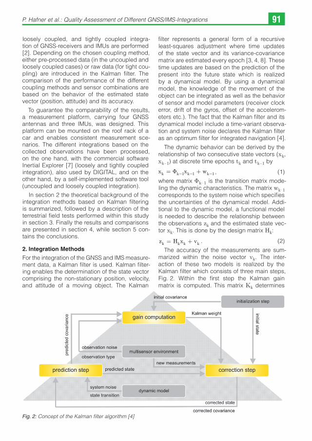
In the field of navigation, integrated navigation is an upcoming technique. This means that the trajectory determination of a moving object is performed by a sensor fusion: for a discrete sequence of epochs, the object-specific state vector and its components (position, velocity and attitude) are derived by an integration of several sensors. In most cases, complementary multi-sensor systems are used. Therefore, sen-sors with different operation principles and char-acteristics complement each other in such a way that disadvantages of the one sensor are com-pensated by the advantages of the other and vice versa [7, 8]. In the case of mobile platforms, the integration of satellite-based positioning and inertial measurement systems is gaining impor-tance today [3]. Global Navigation Satellite Sys-tems (GNSS), such as GPS or the future Galileo, yield absolute positions, but in the sense of radio navigation, they are non-autonomous systems. In contrast, inertial navigation (use of gyroscopes and accelerometers) is self-contained, but pro-vides relative positions [4]. Therefore, the impor-tance of the sensor integration is obvious: an inertial measurement system (IMS) overcomes outages of GNSS, while GNSS compensates the IMS-typical drift behavior. In Table 1 the charac-teristics of GNSS are opposed to the character-istics of IMS.

Within the scope of the project VarIoNav [5], a science-based and comprehensive investigation of different types of GNSS-IMS integration was performed by the Institute of Navigation, Graz University of Technology. The goal of the project was a classification of different integration meth-ods based on different sensor combinations in the frame of the trajectory determination for a mobile exploration system (imaging sensors)

operated by DIGITAL (department Remote Sens-ing and Geoinformation), an institute of JOAN-NEUM RESEARCH, Graz. The investigation should be a basis for investment decisions – are additional costs for high quality sensors really necessary to achieve the desired accuracy?

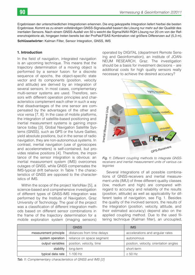
Fig. 1: Different coupling methods to integrate GNSS-receivers and inertial measurement units of various ca-tegories

Several integrations of all possible combina-tions of GNSS-receivers and inertial measure-ment units (IMU) of three different quality classes (low, medium and high) are compared with regard to accuracy and reliability of the results (position, attitude) as well as applicability for dif-ferent tasks of navigation, see Fig. 1. Besides the quality of the involved sensors, the results of the integration (position, velocity, attitude, and their estimated accuracy) depend also on the applied coupling method. Due to the used fil-tering technique (Kalman filter), an uncoupled,

Ergebnissen der unterschiedlichen Integrationen erkennen. Die eng gekoppelte Integration liefert hierbei die besten Ergebnisse. Kommt es zu einem vollständigen GNSS-Signalausfall basiert die Lösung nur mehr auf der Qualität des inertialen Sensors. Nach einem GNSS-Ausfall von 50 s weicht die Sigma/iNAV-RQH Lösung nur 20 cm von der Ref-erenztrajektorie ab, hingegen treten bereits bei der ProPak/FSAS Kombination viel größere Differenzen auf (5,3 m).

Schlüsselwörter: Kalman Filter, Sensor Integration, GNSS, IMS

GNSS IMS

measurement principle distances from time delays accelerations and angular rates

system operation reliance on space segment autonomous

output variables position, velocity, time position, velocity, orientation angles

stability long-term short-term

typical data rate 1-100 Hz ≥ 50 Hz

Tab. 1: Complementary characteristics of GNSS and IMS [2]

P. Hafner et al.: Quality Assessment of Different GNSS/IMS-Integrations 91

loosely coupled, and tightly coupled integra-tion of GNSS-receivers and IMUs are performed [2]. Depending on the chosen coupling method, either pre-processed data (in the uncoupled and loosely coupled cases) or raw data (for tight cou-pling) are introduced in the Kalman filter. The comparison of the performance of the different coupling methods and sensor combinations are based on the behavior of the estimated state vector (position, attitude) and its accuracy.

To guarantee the comparability of the results, a measurement platform, carrying four GNSS antennas and three IMUs, was designed. This platform can be mounted on the roof rack of a car and enables consistent measurement sce-narios. The different integrations based on the collected observations have been processed, on the one hand, with the commercial software Inertial Explorer [7] (loosely and tightly coupled integration), also used by DIGITAL, and on the other hand, by a self-implemented software tool (uncoupled and loosely coupled integration).

In section 2 the theoretical background of the integration methods based on Kalman filtering is summarized, followed by a description of the terrestrial field tests performed within this study in section 3. Finally the results and comparisons are presented in section 4, while section 5 con-tains the conclusions.

2. Integration Methods

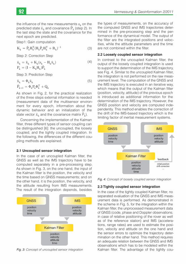
For the integration of the GNSS and IMS measure-ment data, a Kalman filter is used. Kalman filter-ing enables the determination of the state vector comprising the non-stationary position, velocity, and attitude of a moving object. The Kalman

filter represents a general form of a recursive least-squares adjustment where time updates of the state vector and its variance-covariance matrix are estimated every epoch [3, 4, 8]. These time updates are based on the prediction of the present into the future state which is realized by a dynamical model. By using a dynamical model, the knowledge of the movement of the object can be integrated as well as the behavior of sensor and model parameters (receiver clock error, drift of the gyros, offset of the accelerom-eters etc.). The fact that the Kalman filter and its dynamical model include a time-variant observa-tion and system noise declares the Kalman filter as an optimum filter for integrated navigation [4].

The dynamic behavior can be derived by the relationship of two consecutive state vectors (xk, xk–1) at discrete time epochs tk and tk–1 by

x x wk k k k= +− − −Φ 1 1 1 , (1)

where matrix Fk–1 is the transition matrix mode-ling the dynamic characteristics. The matrix wk–1 corresponds to the system noise which specifies the uncertainties of the dynamical model. Addi-tional to the dynamic model, a functional model is needed to describe the relationship between the observations zk and the estimated state vec-tor xk. This is done by the design matrix Hk:

z H x vk k k k= + . (2)

The accuracy of the measurements are sum-marized within the noise vector vk. The inter-action of these two models is realized by the Kalman filter which consists of three main steps, Fig. 2. Within the first step the Kalman gain matrix is computed. This matrix Kk determines

Fig. 2: Concept of the Kalman filter algorithm [4]


the influence of the new measurements zk on the predicted state x̃k and covariance P̃k (step 2). In the last step the state and the covariance for the next epoch are predicted.

Step1: Gain computation

K P H H P H Rk k kT

k k kT

k= + − ( ) 1 (3)

Step 2: Correction Step

ˆ ( )

( )

x x K z H x

P I K H Pk k k k k k

k k k k

= + −= −

(4)

Step 3: Prediction Step

x x

P P Qk k k

k k k kT

k

=

= ++

Φ

Φ Φ

ˆ

1

(5)

As shown in Fig. 2, for the practical realization of the three steps external information is needed (measurement data of the multisensor environ-ment for every epoch, information about the dynamic behavior and an initialization of the state vector x̃k and the covariance matrix P̃k).

Concerning the implementation of the Kalman filter, three different types of sensor coupling can be distinguished [6]: the uncoupled, the loosely coupled, and the tightly coupled integration. In the following, the differences of the different cou-pling methods are explained.

2.1 Uncoupled sensor integration

In the case of an uncoupled Kalman filter, the GNSS as well as the IMS trajectory have to be computed separately in a pre-processing step. As shown in Fig. 3, on the one hand, the input of the Kalman filter is the position, the velocity and the time based on GNSS measurements; and on the other hand, it is the position, the velocity, and the attitude resulting from IMS measurements. The result of the integration depends, besides

the types of measurements, on the accuracy of the computed GNSS and IMS trajectories deter-mined in the pre-processing step and the per-formance of the dynamical model. The output of the filter are the integrated positions and veloc-ities, while the attitude parameters and the time are not combined within the filter.

2.2 Loosely coupled sensor integration

In contrast to the uncoupled Kalman filter, the output of the loosely coupled integration is used to support the determination of the IMS trajectory, see Fig. 4. Similar to the uncoupled Kalman filter, the integration is not performed on the raw meas-urement level. The computation of the GNSS and the IMS trajectory is executed in an iterative way, which means that the output of the Kalman filter (position, velocity, attitude) of the previous epoch is introduced as additional information for the determination of the IMS trajectory. However, the GNSS position and velocity are computed inde-pendently. This method enables the correction of the drift of the IMS-based trajectory which is the limiting factor of inertial measurement systems.

Fig. 4: Concept of loosely coupled sensor integration

2.3 Tightly coupled sensor integration

In the case of the tightly coupled Kalman filter, no separated evaluation of the GNSS and IMS meas-urement data is performed. As demonstrated in the scheme in Fig. 5, for the integration within the Kalman filter, the unprocessed measurement data of GNSS (code, phase and Doppler observations; in case of relative positioning of the rover as well as of the reference station) and IMS (accelera-tions, range rates) are used to estimate the posi-tion, velocity and attitude on the one hand and the sensor errors to optimize the trajectory deter-mination on the other hand. This method requires an adequate relation between the GNSS and IMS observations which has to be modeled within the Kalman filter. The advantage of the tightly cou-Fig. 3: Concept of uncoupled sensor integration


pled sensor integration is that the output of the fil-ter (estimated parameters) and the Kalman filter model itself support the trajectory determination by means of solving the phase ambiguities and applying the estimated IMU sensor errors (gyro drift [9], accelerometer biases, misalignment …). The modeling of all correlations and relations between the GNSS and IMS data results in a very complex filter design.

Fig. 5: Concept of tightly coupled sensor integration

The tightly coupled integration has, among oth-ers, the essential advantage that also absolute position solutions with less than four observa-ble satellites can be computed, since the absent observations are compensated by the comple-mentary measurement system (IMS).

3. Terrestrial field tests

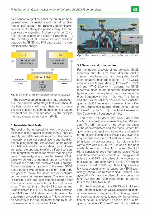
The goal of the investigations was the accuracy estimation of the navigation components (position, velocity and attitude) with regard to the various measurement sensor combinations and the differ-ent coupling methods. The analysis of the results and their estimated accuracy should give informa-tion about the applicability of the different sensors and integration methods for mobile mapping sys-tems. These analyses are based on terrestrial field tests which were performed under varying cir-cumstances (partly and complete GNSS outage). For a consistent comparison of the used GNSS receivers and IMS sensors, a platform had to be designed to realize the same sensor configura-tion for every test measurement. The equipment is fixed to a stiff and light-weighted carbon-fiber frame which can be mounted on the roof rack of a car. The mounting of the GNSS-antennas and IMUs is shown in Fig. 6. The lever arms between the GNSS and IMU reference points have to be determined as good as possible. This is done with an accuracy in the sub millimeter range by terres-trial measurements with a theodolite.

Fig. 6: Measurement platform mounted on the roof rack of a car

3.1 Sensors and observables

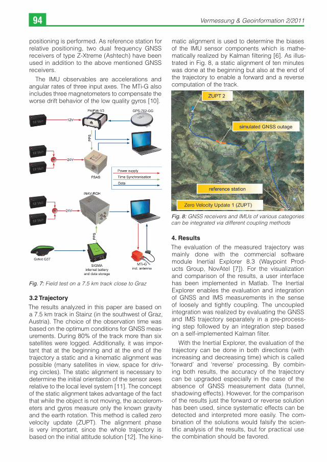
For the quality analysis of the sensors, GNSS receivers and IMUs of three different quality classes have been used and integrated via dif-ferent coupling methods (see Fig. 7). The GNSS receivers are Sigma (Javad), ProPak-V3 (NovA-tel) and MTi-G (Xsens). In general, the GNSS receivers differ in the recorded measurement types (code, carrier phase) and their measure-ment frequency (4 Hz – 100 Hz). The Sigma and the ProPak-V3 receivers are both dual fre-quency GNSS receivers, however they differ in the update rate (Sigma offers up to 100 Hz, ProPak-V3 up to 50 Hz). The MTi-G measures C/A-Code with a frequency of 4 Hz.

The iNav-RQH (iMAR), the FSAS (iMAR) and the MTi-G (Xsens) are representing the IMU sen-sors. The drift behavior of the gyros, the offset of the accelerometers and the measurement fre-quency are among other parameters responsible for the classification of the IMUs. iNav-RQH is a very precise measurement system, whose RLGs (ring laser gyros) possess a high bias stability with a gyro-drift of 0.003°/h. It is one of the best available sensors on the IMU market. The IMU FSAS consists of three fiber optical gyros (FOG) and three servo-accelerometers. The gyro-drift is less than 0.75°/h, the offset of the accelerome-ters is about 1 mg (compared to iNav-RQH which shows an offset of 0.06 mg). MTi-G represents a low-cost system which is based on MEMS tech-nology (Micro Electro Mechanical System). The gyro-drift (1°/h) and the offset of the accelerome-ters (100 mg) are much worse than the parame-ters of the other two IMUs.

For the integration of the GNSS and IMU sen-sors, different types of GNSS positioning meth-ods are involved. Single point positioning based on code measurements is used for the combina-tion of the MTi-G sensors. In case of the dual fre-quency receivers ProPak-V3 and Sigma relative


positioning is performed. As reference station for relative positioning, two dual frequency GNSS receivers of type Z-Xtreme (Ashtech) have been used in addition to the above mentioned GNSS receivers.

The IMU observables are accelerations and angular rates of three input axes. The MTi-G also includes three magnetometers to compensate the worse drift behavior of the low quality gyros [10].

Fig. 7: Field test on a 7.5 km track close to Graz

3.2 Trajectory

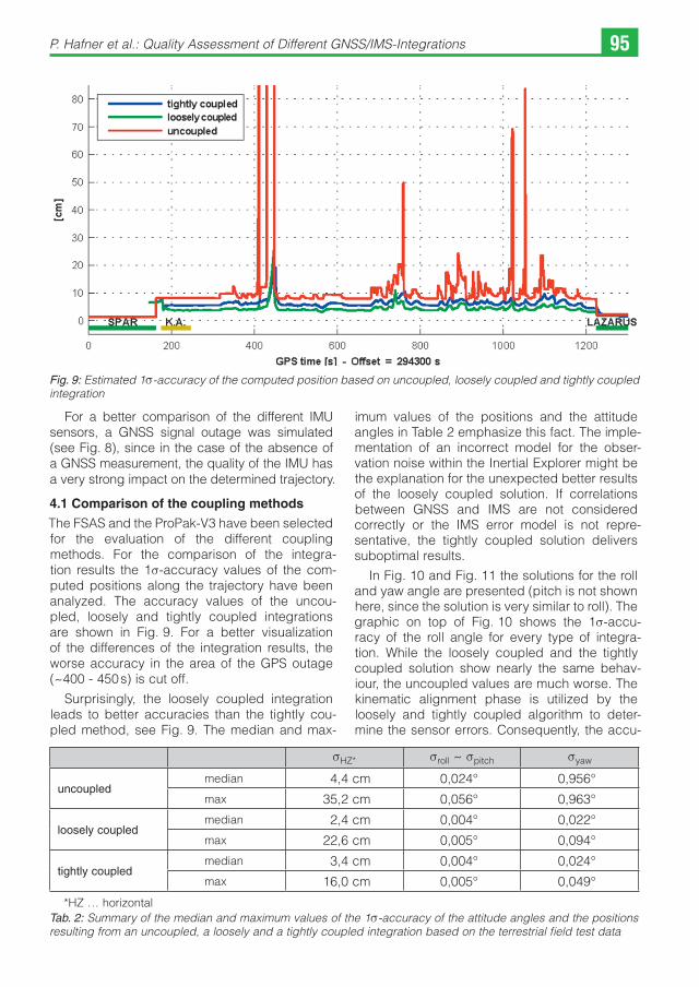
The results analyzed in this paper are based on a 7.5 km track in Stainz (in the southwest of Graz, Austria). The choice of the observation time was based on the optimum conditions for GNSS meas-urements. During 80% of the track more than six satellites were logged. Additionally, it was impor-tant that at the beginning and at the end of the trajectory a static and a kinematic alignment was possible (many satellites in view, space for driv-ing circles). The static alignment is necessary to determine the initial orientation of the sensor axes relative to the local level system [11]. The concept of the static alignment takes advantage of the fact that while the object is not moving, the accelerom-eters and gyros measure only the known gravity and the earth rotation. This method is called zero velocity update (ZUPT). The alignment phase is very important, since the whole trajectory is based on the initial attitude solution [12]. The kine-

matic alignment is used to determine the biases of the IMU sensor components which is mathe-matically realized by Kalman filtering [6]. As illus-trated in Fig. 8, a static alignment of ten minutes was done at the beginning but also at the end of the trajectory to enable a forward and a reverse computation of the track.

Fig. 8: GNSS receivers and IMUs of various categories can be integrated via different coupling methods

4. Results

The evaluation of the measured trajectory was mainly done with the commercial software module Inertial Explorer 8.3 (Waypoint Prod-ucts Group, NovAtel [7]). For the visualization and comparison of the results, a user interface has been implemented in Matlab. The Inertial Explorer enables the evaluation and integration of GNSS and IMS measurements in the sense of loosely and tightly coupling. The uncoupled integration was realized by evaluating the GNSS and IMS trajectory separately in a pre-process-ing step followed by an integration step based on a self-implemented Kalman filter.

With the Inertial Explorer, the evaluation of the trajectory can be done in both directions (with increasing and decreasing time) which is called ‘forward’ and ‘reverse’ processing. By combin-ing both results, the accuracy of the trajectory can be upgraded especially in the case of the absence of GNSS measurement data (tunnel, shadowing effects). However, for the comparison of the results just the forward or reverse solution has been used, since systematic effects can be detected and interpreted more easily. The com-bination of the solutions would falsify the scien-tific analysis of the results, but for practical use the combination should be favored.


For a better comparison of the different IMU sensors, a GNSS signal outage was simulated (see Fig. 8), since in the case of the absence of a GNSS measurement, the quality of the IMU has a very strong impact on the determined trajectory.

4.1 Comparison of the coupling methods

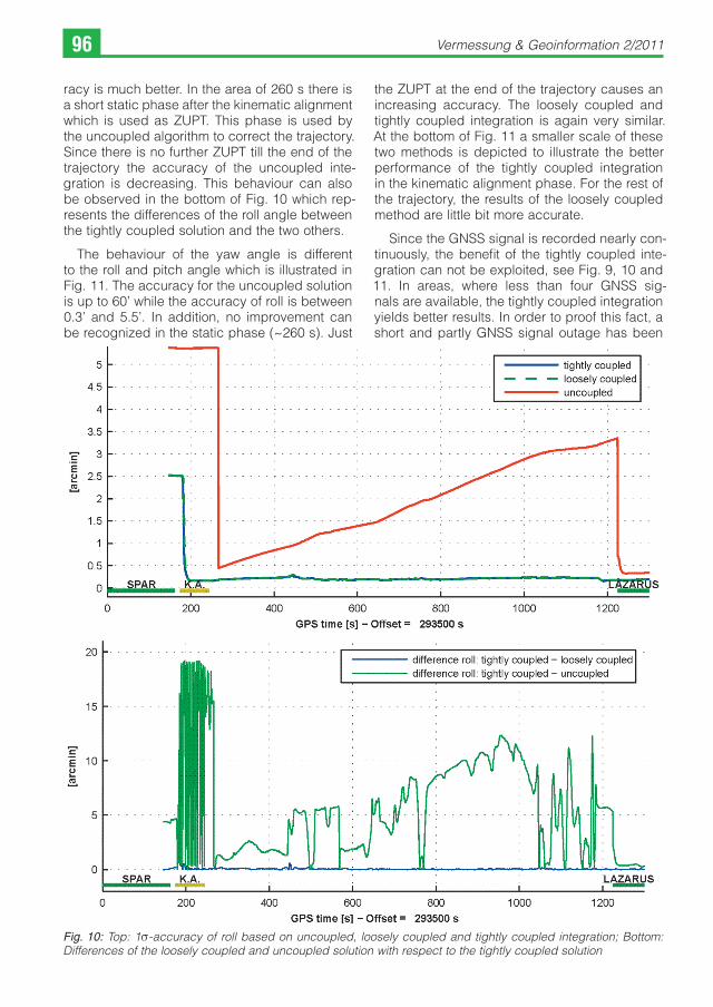
The FSAS and the ProPak-V3 have been selected for the evaluation of the different coupling methods. For the comparison of the integra-tion results the 1s-accuracy values of the com-puted positions along the trajectory have been analyzed. The accuracy values of the uncou-pled, loosely and tightly coupled integrations are shown in Fig. 9. For a better visualization of the differences of the integration results, the worse accuracy in the area of the GPS outage (~400 - 450 s) is cut off.

Surprisingly, the loosely coupled integration leads to better accuracies than the tightly cou-pled method, see Fig. 9. The median and max-

imum values of the positions and the attitude angles in Table 2 emphasize this fact. The imple-mentation of an incorrect model for the obser-vation noise within the Inertial Explorer might be the explanation for the unexpected better results of the loosely coupled solution. If correlations between GNSS and IMS are not considered correctly or the IMS error model is not repre-sentative, the tightly coupled solution delivers suboptimal results.

In Fig. 10 and Fig. 11 the solutions for the roll and yaw angle are presented (pitch is not shown here, since the solution is very similar to roll). The graphic on top of Fig. 10 shows the 1s-accu-racy of the roll angle for every type of integra-tion. While the loosely coupled and the tightly coupled solution show nearly the same behav-iour, the uncoupled values are much worse. The kinematic alignment phase is utilized by the loosely and tightly coupled algorithm to deter-mine the sensor errors. Consequently, the accu-

Fig. 9: Estimated 1s-accuracy of the computed position based on uncoupled, loosely coupled and tightly coupled integration

sHZ* sroll ~ spitch syaw

uncoupledmedian 4,4 cm 0,024° 0,956°

max 35,2 cm 0,056° 0,963°

loosely coupledmedian 2,4 cm 0,004° 0,022°

max 22,6 cm 0,005° 0,094°

tightly coupledmedian 3,4 cm 0,004° 0,024°

max 16,0 cm 0,005° 0,049°

*HZ … horizontalTab. 2: Summary of the median and maximum values of the 1s-accuracy of the attitude angles and the positions resulting from an uncoupled, a loosely and a tightly coupled integration based on the terrestrial field test data


racy is much better. In the area of 260 s there is a short static phase after the kinematic alignment which is used as ZUPT. This phase is used by the uncoupled algorithm to correct the trajectory. Since there is no further ZUPT till the end of the trajectory the accuracy of the uncoupled inte-gration is decreasing. This behaviour can also be observed in the bottom of Fig. 10 which rep-resents the differences of the roll angle between the tightly coupled solution and the two others.

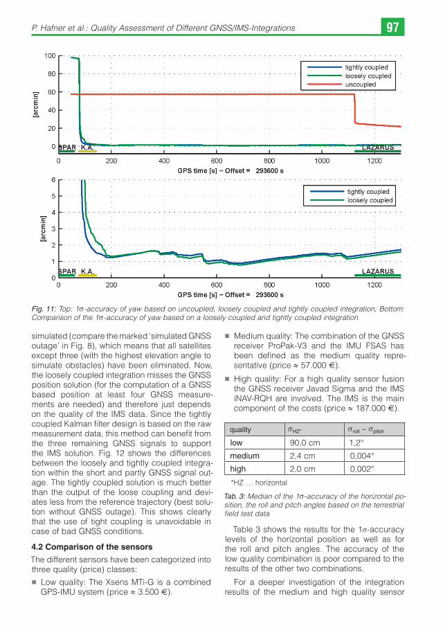
The behaviour of the yaw angle is different to the roll and pitch angle which is illustrated in Fig. 11. The accuracy for the uncoupled solution is up to 60’ while the accuracy of roll is between 0.3’ and 5.5’. In addition, no improvement can be recognized in the static phase (~260 s). Just

the ZUPT at the end of the trajectory causes an increasing accuracy. The loosely coupled and tightly coupled integration is again very similar. At the bottom of Fig. 11 a smaller scale of these two methods is depicted to illustrate the better performance of the tightly coupled integration in the kinematic alignment phase. For the rest of the trajectory, the results of the loosely coupled method are little bit more accurate.

Since the GNSS signal is recorded nearly con-tinuously, the benefit of the tightly coupled inte-gration can not be exploited, see Fig. 9, 10 and 11. In areas, where less than four GNSS sig-nals are available, the tightly coupled integration yields better results. In order to proof this fact, a short and partly GNSS signal outage has been

Fig. 10: Top: 1s-accuracy of roll based on uncoupled, loosely coupled and tightly coupled integration; Bottom: Differences of the loosely coupled and uncoupled solution with respect to the tightly coupled solution


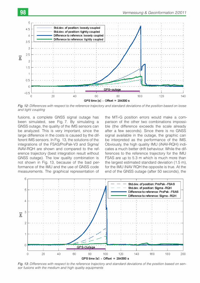
simulated (compare the marked ‘simulated GNSS outage’ in Fig. 8), which means that all satellites except three (with the highest elevation angle to simulate obstacles) have been eliminated. Now, the loosely coupled integration misses the GNSS position solution (for the computation of a GNSS based position at least four GNSS measure-ments are needed) and therefore just depends on the quality of the IMS data. Since the tightly coupled Kalman filter design is based on the raw measurement data, this method can benefit from the three remaining GNSS signals to support the IMS solution. Fig. 12 shows the differences between the loosely and tightly coupled integra-tion within the short and partly GNSS signal out-age. The tightly coupled solution is much better than the output of the loose coupling and devi-ates less from the reference trajectory (best solu-tion without GNSS outage). This shows clearly that the use of tight coupling is unavoidable in case of bad GNSS conditions.

4.2 Comparison of the sensors

The different sensors have been categorized into three quality (price) classes:

� Low quality: The Xsens MTi-G is a combined GPS-IMU system (price ≈ 3.500 €).

� Medium quality: The combination of the GNSS receiver ProPak-V3 and the IMU FSAS has been defined as the medium quality repre-sentative (price ≈ 57.000 €).

� High quality: For a high quality sensor fusion the GNSS receiver Javad Sigma and the IMS iNAV-RQH are involved. The IMS is the main component of the costs (price ≈ 187.000 €).

quality sHZ* sroll ~ spitch

low 90,0 cm 1,2°

medium 2,4 cm 0,004°

high 2,0 cm 0,002°

*HZ … horizontal

Tab. 3: Median of the 1s-accuracy of the horizontal po-sition, the roll and pitch angles based on the terrestrial field test data

Table 3 shows the results for the 1s-accuracy levels of the horizontal position as well as for the roll and pitch angles. The accuracy of the low quality combination is poor compared to the results of the other two combinations.

For a deeper investigation of the integration results of the medium and high quality sensor

Fig. 11: Top: 1s-accuracy of yaw based on uncoupled, loosely coupled and tightly coupled integration; Bottom: Comparison of the 1s-accuracy of yaw based on a loosely coupled and tightly coupled integration


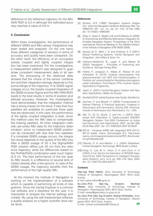
fusions, a complete GNSS signal outage has been simulated, see Fig. 7. By simulating a GNSS outage, the quality of the IMS sensors can be analyzed. This is very important, since the large difference in the costs is caused by the dif-ferent IMS sensors. In Fig. 13, the solutions of the integrations of the FSAS/ProPak-V3 and Sigma/iNAV-RQH are shown and compared to the ref-erence trajectory (best integration result without GNSS outage). The low quality combination is not shown in Fig. 13, because of the bad per-formance of the IMU and the use of GNSS code measurements. The graphical representation of

the MTi-G position errors would make a com-parison of the other two combinations impossi-ble (the difference exceeds the scale already after a few seconds). Since there is no GNSS signal available in the outage, the graphic can be interpreted as the performance of the IMS. Obviously, the high quality IMU (iNAV-RQH) indi-cates a much better drift behaviour. While the dif-ferences to the reference trajectory for the IMU FSAS are up to 5.3 m which is much more than the largest estimated standard deviation (1.5 m), for the IMU iNAV RQH the opposite is true. At the end of the GNSS outage (after 50 seconds), the

Fig. 12: Differences with respect to the reference trajectory and standard deviations of the position based on loose and tight coupling

Fig. 13: Differences with respect to the reference trajectory and standard deviations of the position based on sen-sor fusions with the medium and high quality equipments


difference to the reference trajectory for the IMU iNAV RQH is 0.2 m although the estimated accu-racy reaches a value of 0.8 m.

5. Conclusion

Within these investigations, the performance of different GNSS and IMU sensor integrations has been tested and analyzed. On the one hand, three different categories of sensors in terms of accuracy and quality have been compared. On the other hand, the efficiency of an uncoupled, loosely coupled and tightly coupled integra-tion has been examined. For the investigations, a measurement platform was designed to guar-antee consistent measurement data of all sen-sors. The processing of the observed data showed that the choice of the sensor combina-tion and their integration strongly depends on the surroundings of the trajectory. If no GNSS signal outages occur, the loosely coupled integration of the GNSS receiver Sigma and the IMU iNAV-RQH leads to the best results in terms of position and attitude accuracy. However, the investigations have demonstrated, that the integration method has a strong impact on the result, if less than four satellites are available (in particular three satel-lites are observed). In this case, the performance of the tightly coupled integration is best, since this method uses the IMU data to compensate the missing satellites. All other integration meth-ods use solely IMU data for the trajectory deter-mination, since no independent GNSS position can be computed with less than four satellites. If a complete GNSS outage occurs, the integra-tion result depends on the quality of the IMU only. After a GNSS outage of 50 s the Sigma/iNAV-RQH solution differs just 20 cm from the refer-ence trajectory, while the differences based on the ProPak/FSAS combination were much higher (5.3 m). The bad performance of the low qual-ity IMU results in a difference of several tens of meters already after a few epochs. In case of the GNSS outage, the trajectory benefits from the performance of the high quality IMU.

At the moment the Institute of Navigation is working on the implementation of a software which is capable of performing all kinds of inte-grations. Since the Inertial Explorer is a commer-cial software and a blackbox for the user, it is impossible to analyse the internal settings and models. By using the self-implemented software, a quality analysis on a higher scientific level can be done.

References

[1] Gordon, G.S. (1998): Navigation systems integra-tion. Airborne Navigation Systems Workshop (Ref. No. 1998/275), IEE , vol., no., pp. 4/1- 416, 10 Feb 1998. doi: 10.1049/ic:19980390

[2] Zhao, X., Syed, Z., Wright, D.B. and El-Sheimy, N. (2009): An Economical and Effective Multi-sensor Integration for Portable Navigation System. Proceedings of the 22nd International Technical Meeting of The Satellite Division of the Institute of Navigation (ION GNSS 2009).

[3] Grewal, M. S., Weill, L. R. and Andrews, A. P. (2001): Global Positioning Systems, Inertial Navigation and Integration. John Wiley & Sons, Inc.

[4] Hofmann-Wellenhof, B., Legat, K. and Wieser, M. (2003): Navigation – Principles of Positioning and Guidance. Springer-Verlag Wien.

[5] Hafner, P., Längauer, K., Wasle, B., Wieser, M. and Kühtreiber, N. (2010): Analyse verschiedener Inte-grationsvarianten von GPS und Inertialnavigation in Hinblick auf unterschiedliche Georeferenzierungssze-narien (VarIoNav). Final Report, FFG, Austrian Space Applications Programme.

[6] Jekeli, C. (2001): Inertial Navigation System with Geo-detic Applications. Walter de Gruyter.

[7] NovAtel (2010): Inertial Explorer User Guide. NovAtel Inc.

[8] Zarchan, P. and Musoff, H. (2005): Fundamentals of Kalman Filtering: A Practical Approach. Progress in Astronautics and Aeronautics. Volume 208. American Insitute of Aeronautics and Astronautics, Inc., USA.

[9] Wei, G.; Qi, N,; Guofu, Z. and Hui, J. (2007): Gyro-scope Drift Estimation in Tightly-coupled INS/GPS Navigation System. 2nd IEEE Conference on Indus-trial Electronics and Applications, 2007. pp.391-396, 23-25 May 2007. doi: 10.1109/ICIEA.2007.4318437.

[10] MTi-G – miniature AHRS with integrated GPS (2011):. MTi-G leaflet. Xsens Technologies B.V. http://www.xsens.com/images/stories/products/PDF_Brochures/mti-g%20leaflet.pdf

[11] Titterton, D. H. and Weston, J. L. (2004): Strapdown Inertial Navigation Technology. MPG Books Limited.

[12] Hong, S., Lee, M. H., Kwon, S. H. and Chun, H. H. (2004): A Car Test for the Estimation of GPS/INS Align-ment Errors. IEEE Transactions on Intelligent Transpor-tation Systems, vol.5, no.3, pp. 208- 218, Sept. 2004. doi: 10.1109/TITS.2004.833771.

Contacts

Dipl.-Ing. Petra Hafner, Graz University of Technology, Institute of Navigation, Steyrergasse 30/III, 8010 Graz, Austria. E-mail: [email protected]. Dipl.-Ing. Dr.techn. Manfred Wieser, Graz University of Technology, Institute of Navigation, Steyrergasse 30/III, 8010 Graz, Austria. E-mail: [email protected]. Dipl.-Ing. Dr.techn. Norbert Kühtreiber, Graz University of Technology, Institute of Navigation, Steyrer-gasse 30/III, 8010 Graz, Austria. E-mail: [email protected]

Documents

MTiG 05 Hafner-wieser-kuehtreiber