Multi-Dimensional Transfer Functions for Interactive Volume RenderingJoe Kniss Gordon Kindlmann Charles Hansen

Scientific Computing and Imaging InstituteSchool of Computing, University of Utahfjmkjgkjhanseng@cs.utah.edu

1 Abstract

Most direct volume renderings produced today employ one-dimensional transfer functions, which assign color and opacity tothe volume based solely on the single scalar quantity which com-prises the dataset. Though they have not received widespread atten-tion, multi-dimensional transfer functions are a very effective wayto extract materials and their boundaries for both scalar and mul-tivariate data. However, identifying good transfer functions is dif-ficult enough in one dimension, let alone two or three dimensions.This paper demonstrates an important class of three-dimensionaltransfer functions for scalar data, and describes the applicationof multi-dimensional transfer functions to multivariate data. Wepresent a set of direct manipulation widgets that make specifyingsuch transfer functions intuitive and convenient. We also describehow to use modern graphics hardware to both interactively renderwith multi-dimensional transfer functions and to provide interactiveshadows for volumes. The transfer functions, widgets, and hard-ware combine to form a powerful system for interactive volumeexploration.Keywords: volume visualization, direct volume rendering, multi-dimensional transfer functions, direct manipulation widgets, graph-ics hardware

2 Introduction

Direct volume rendering has proven to be an effective and flexi-ble visualization method for three-dimensional (3D) scalar fields.Transfer functions are fundamental to direct volume rendering be-cause their role is essentially to make the data visible: by assigningoptical properties like color and opacity to the voxel data, the vol-ume can be rendered with traditional computer graphics methods.Good transfer functions reveal the important structures in the datawithout obscuring them with unimportant regions. To date, transferfunctions have generally been limited to one-dimensional (1D) do-mains, meaning that the 1D space of scalar data value has been theonly variable to which opacity and color are assigned. One aspectof direct volume rendering which has received little attention is theuse of multi-dimensional transfer functions.

Often, there are features of interest in volume data that are dif-ficult to extract and visualize with 1D transfer functions. Manymedical datasets created from CT or MRI scans contain a complexcombination of boundaries between multiple materials. This situ-ation is problematic for 1D transfer functions because of the po-tential for overlap between the data value intervals spanned by thedifferent boundaries. When one data value is associated with mul-tiple boundaries, a 1D transfer function is unable to render them inisolation. Another benefit of higher dimensional transfer functionsis their ability to portray subtle variations in properties of a singleboundary, such as its thickness. When working with multivariatedata, a similar difficulty arises with features that can be identifiedonly by their unique combination of multiple data values. A 1Dtransfer function is simply not capable of capturing this relation-ship.

Unfortunately, using multi-dimensional transfer functions in vol-ume rendering is complicated. Even when the transfer functionis only 1D, finding an appropriate transfer function is generallyaccomplished by trial and error. This is one of the main chal-lenges in making direct volume rendering an effective visualizationtool. Adding dimensions to the transfer function domain only com-pounds the problem. While this is an ongoing research area, manyof the proposed methods for transfer function generation and ma-nipulation are not easily extended to higher dimensional transferfunctions. In addition, fast volume rendering algorithms that as-sume the transfer function can be implemented as a linear lookuptable (LUT) can be difficult to adapt to multi-dimensional transferfunctions due to the linear interpolation imposed on such LUTs.

A previous paper [19] demonstrated the importance and power ofmulti-dimensional transfer functions. This paper extends that workwith a more detailed exposition of the multi-dimensional trans-fer function concept, a generalization of multi-dimensional trans-fer functions for both scalar and multivariate data, as well as anovel technique for the interactive generation of volumetric shad-ows. To resolve the potential complexities in a user interface formulti-dimensional transfer functions, we introduce a set of directmanipulation widgets which make finding and experimenting withtransfer functions an intuitive, efficient, and informative process.In order to make this process genuinely interactive, we exploit thefast rendering capabilities of modern graphics hardware, especially3D texture memory and pixel texturing operations. Together, thewidgets and the hardware form the basis for new interaction modeswhich can guide users towards transfer function settings appropri-ate for their visualization and data exploration interests.

3 Previous Work3.1 Transfer Functions

Even though volume rendering as a visualization tool is more thanten years old, only recently has research focused on making thespace of transfer functions easier to explore. He et al. [12] gener-ated transfer functions with genetic algorithms driven either by userselection of thumbnail renderings, or some objective image fitnessfunction. The Design Gallery [26] creates an intuitive interface tothe entire space of all possible transfer functions based on auto-mated analysis and layout of rendered images. A more data-centricapproach is the Contour Spectrum [1], which visually summarizesthe space of isosurfaces in terms of metrics like surface area andmean gradient magnitude, thereby guiding the choice of isovaluefor isosurfacing, and also providing information useful for trans-fer function generation. Another recent paper [21] presents a noveltransfer function interface in which small thumbnail renderings arearranged according to their relationship with the spaces of data val-ues, color, and opacity.

The application of these methods is limited to the generation of1D transfer functions, even though 2D transfer functions were in-troduced by Levoy in 1988 [25]. Levoy introduced two styles oftransfer functions, both two-dimensional, and both using gradientmagnitude for the second dimension. One transfer function wasintended for the display of interfaces between materials, the other

for the display of isovalue contours in more smoothly varying data.The previous work most directly related to our approach for visu-alizing scalar data facilitates the semi-automatic generation of both1D and 2D transfer functions [17, 32]. Using principles of com-puter vision edge detection, the semi-automatic method strives toisolate those portions of the transfer function domain which mostreliably correlate with the middle of material interface boundaries.Other work closely related to our approach for visualizing multi-variate data uses a 2D transfer function to visualize data derivedfrom multiple MRI pulse sequences [23].

Scalar volume rendering research that uses multi-dimensionaltransfer functions is relatively scarce. One paper discusses the useof transfer functions similar to Levoy’s as part of visualization inthe context of wavelet volume representation [30]. More recently,the VolumePro graphics board uses a 12-bit 1D lookup table forthe transfer function, but also allows opacity modulation by gra-dient magnitude, effectively implementing a separable 2D trans-fer function [31]. Other work involving multi-dimensional transferfunctions uses various types of second derivatives in order to distin-guish features in the volume according to their shape and curvaturecharacteristics [15, 37].

Designing colormaps for displaying non-volumetric data is atask similar to finding transfer functions. Previous work has de-veloped strategies and guidelines for colormap creation, based onvisualization goals, types of data, perceptual considerations, anduser studies [3, 35, 39].

3.2 Direct Manipulation Widgets

Direct manipulation widgets are geometric objects rendered with avisualization and are designed to provide the user with a 3D inter-face [5, 14, 34, 38, 41]. For example, a frame widget can be usedto select a 2D plane within a volume. Widgets are typically ren-dered from basic geometric primitives such as spheres, cylinders,and cones. Widget construction is often guided by a constraint sys-tem which binds elements of a widget to one another. Each sub-partof a widget represents some functionality of the widget or a param-eter to which the user has access.

3.3 Hardware Volume Rendering

Many volume rendering techniques based on graphics hardware uti-lize texture memory to store a 3D dataset. The dataset is then sam-pled, classified, rendered to proxy geometry, and composited. Clas-sification typically occurs in hardware as a 1D table lookup.

2D texture-based techniques slice along the major axes of thedata and take advantage of hardware bilinear interpolation withinthe slice [4]. These methods require three copies of the volume toreside in texture memory, one per axis, and they often suffer fromartifacts caused by under-sampling along the slice axis. Trilinear in-terpolation can be attained using 2D textures with specialized hard-ware extensions available on some commodity graphics cards [6].This technique allows intermediate slices along the slice axis to becomputed in hardware. These hardware extensions also permit dif-fuse shaded volumes to be rendered at interactive frame rates.

3D texture-based techniques typically sample view-alignedslices through the volume, leveraging hardware trilinear interpo-lation [11]. Other proxy geometry, such as spherical shells, may beused with 3D texture methods to eliminate artifacts caused by per-spective projection [24]. The pixel texture OpenGL extension hasbeen used with 3D texture techniques to encode both data value anda diffuse illumination parameter which allows shading and classi-fication to occur in the same look-up [28]. Engel et al. showedhow to significantly reduce the number of slices needed to ade-quately sample a scalar volume, while maintaining a high qualityrendering, using a mathematical technique of pre-integration andhardware extensions such as dependent textures [10].

Another form of volume rendering graphics hardware is theCube-4 architecture [33] and the subsequent VolumePro PCI graph-ics board [31]. The VolumePro graphics board implements ray cast-ing combined with the shear warp factorization for volume render-ing [22]. It features trilinear interpolation with supersampling, gra-dient estimation, shaded volumes, and provides interactive framerates for scalar volumes with sizes up to 5123 .

4 Multi-Dimensional Transfer Functions

Transfer function specification is arguably the most important taskin volume visualization. While the transfer function’s role is sim-ply to assign optical properties such as opacity and color to thedata being visualized, the value of the resulting visualization willbe largely dependent on how well these optical properties capturefeatures of interest. Specifying a good transfer function can be adifficult and tedious task for several reasons. First, it is difficultto uniquely identify features of interest in the transfer function do-main. Even though a feature of interest may be easily identifiablein the spatial domain, the range of data values that characterize thefeature may be difficult to isolate in the transfer function domaindue to the fact that other, uninteresting regions, may contain thesame range of data values. Second, transfer functions can have anenormous number of degrees of freedom. Even simple 1D trans-fer functions using linear ramps require two degrees of freedom percontrol point. Third, typical user interfaces do not guide the user insetting these control points based on dataset specific information.Without this type of information, the user must rely on trial and er-ror. This kind of interaction can be especially frustrating since smallchanges to the transfer function can result in surprisingly large andunintuitive changes to the volume rendering.

Rather than classifying a sample based on a single scalar value,multi-dimensional transfer functions allow a sample to be classi-fied based on a combination of values. Multiple data values tendincrease the probability that a feature can be uniquely isolated inthe transfer function domain, effectively providing a larger vocabu-lary for expressing the differences between structures in the dataset.These values are the axes of a multi-dimensional transfer function.Adding dimensions to the transfer function, however, greatly in-creases the degrees of freedom necessary for specifying a transferfunction and the need for dataset specific guidance.

In the following sections, we demonstrate the application ofmulti-dimensional transfer functions to two distinct classes of data:scalar data and multivariate data. The scalar data application isfocused on locating surface boundaries in a scalar volume. Wemotivate and describe the axes of the multi-dimensional transferfunction for this type data. We then describe the use of multi-dimensional transfer functions for multivariate data. We use two ex-amples, color volumes and meteorological simulations, to demon-strate the effectiveness of such transfer functions.

4.1 Scalar Data

For scalar data, the gradient is a first derivative measure. As a vec-tor, it describes the direction of greatest change. The normalizedgradient is often used as the normal for surface based volume shad-ing. The gradient magnitude is a scalar quantity which describesthe local rate of change in the scalar field. For notational conve-nience, we will use f 0 to indicate the magnitude of the gradient off , where f is the scalar function representing the data:

f0 = krfk (1)

This value is useful as an axis of the transfer function since itdiscriminates between homogeneous regions (low gradient mag-nitudes) and regions of change (high gradient magnitudes). This

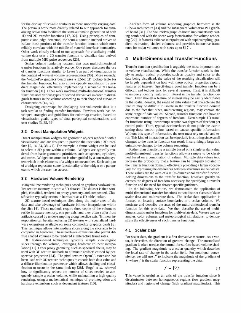
A B C

(a) A 1D histogram. The black region represents the number of datavalue occurrences on a linear scale, the grey is on a log scale. Thecolored regions (A,B,C) identify basic materials.

A B C

D E

Ff '

Data Value(b) A log-scale 2D joint histogram. The lower image shows the locationof materials (A,B,C), and material boundaries (D,E,F).

B

C

E

D

F

(c) A volume rendering showing all of the materials and boundariesidentified above, except air (A), using a 2D transfer function.

Figure 1: Material and boundary identification of the Chapel HillCT Head with data value alone (a) versus data value and gradientmagnitude (f ’), seen in (b). The basic materials captured by CT,air (A), soft tissue (B), and bone (C) can be identified using a 1Dtransfer function as seen in (a). 1D transfer functions, however,cannot capture the complex combinations of material boundaries;air and soft tissue boundary (D), soft tissue and bone boundary (E),and air and bone boundary (F) as seen in (b) and (c).

(a) 1D transfer function (b) 2D transfer function

Figure 2: The frontal and maxillary sinuses of the Visible Male CT.While a 1D transfer function can show the sinuses along with theskin, it cannot capture them in isolation. Only a higher dimensionaltransfer function, in this case a 2D transfer function using data valueand gradient magnitude, can uniquely classify them.

effect can be seen in Figure 1. Figure 1(a) shows a 1D histogrambased on data value and identifies the three basic materials in theChapel Hill CT Head; air (A), soft tissue (B), and bone (C). Fig-ure 1(b) shows a log-scale joint histogram of data value versus gra-dient magnitude. Since materials are relatively homogeneous, theirgradient magnitudes are low. They can be seen as the circular re-gions at the bottom of the histogram. The boundaries between thematerials are shown as the arches; air and soft tissue boundary (D),soft tissue and bone boundary (E), and air and bone boundary (F).Each of these materials and boundaries can be isolated using a 2Dtransfer function based on data value and gradient magnitude. Fig-ure 1(c) shows a volume rendering with the corresponding featureslabeled. The air/bone boundary, (F) in Figure 1 is a good example ofa surface which cannot be isolated using a simple 1D transfer func-tion. This type of boundary appears in CT datasets as the sinusesand mastoid cells. Figure 2 compares attempts at emphasizing thefrontal and maxillary sinuses of the Visible Male CT using a 1Dtransfer function and a 2D transfer function.

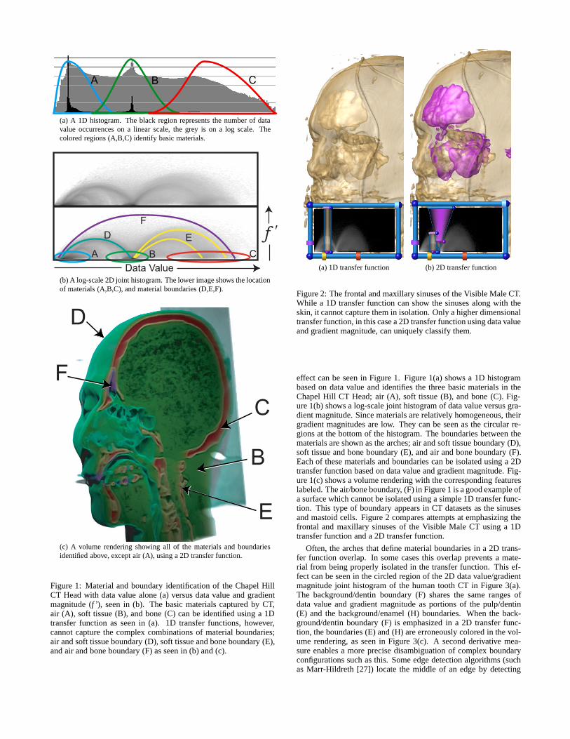
Often, the arches that define material boundaries in a 2D trans-fer function overlap. In some cases this overlap prevents a mate-rial from being properly isolated in the transfer function. This ef-fect can be seen in the circled region of the 2D data value/gradientmagnitude joint histogram of the human tooth CT in Figure 3(a).The background/dentin boundary (F) shares the same ranges ofdata value and gradient magnitude as portions of the pulp/dentin(E) and the background/enamel (H) boundaries. When the back-ground/dentin boundary (F) is emphasized in a 2D transfer func-tion, the boundaries (E) and (H) are erroneously colored in the vol-ume rendering, as seen in Figure 3(c). A second derivative mea-sure enables a more precise disambiguation of complex boundaryconfigurations such as this. Some edge detection algorithms (suchas Marr-Hildreth [27]) locate the middle of an edge by detecting

a zero-crossing in a second derivative measure, such as the Lapla-cian. We compute a more accurate but computationally expensivemeasure, the second directional derivative along the gradient direc-tion, which involves the Hessian (H), a matrix of second partialderivatives. We will use f 00 to indicate this second derivative.

f00 =

1

krfk2(rf)THfrf (2)

More details on these measurements can be found in previouswork on semi-automatic transfer function generation [16, 17]. Fig-ure 3(b) shows a joint histogram of data value verses this second di-rectional derivative. Notice that the boundaries (E), (F), and (G) nolonger overlap. By reducing the opacity assigned to non-zero sec-ond derivative values, we can render the background/dentin bound-ary in isolation, as seen in Figure 3(d). The relationship betweendata value, gradient magnitude, and the second directional deriva-tive is made clear in Figure 4. Figure 4(a) shows the behavior ofthese values along a line through an idealized boundary betweentwo homogeneous materials (inset). Notice that at the center of theboundary, the gradient magnitude is high and the second derivativeis zero. Figure 4(b) shows the behavior of the gradient magnitudeand second derivative as a function of data value. This shows thecurves as they appear in a joint histogram or a transfer function.

4.2 Multivariate data

Multivariate data contains, at each sample point, multiple scalar val-ues that represent different simulated or measured quantities. Mul-tivariate data can come from numerical simulations which calcu-late a list of quantities at each timestep, or from medical scanningmodalities such as MRI, which can measure a variety of tissue char-acteristics, or from a combination of different scanning modalities,such as MRI, CT, and PET. Multi-dimensional transfer functionsare an obvious choice for volume visualization of multivariate data,since we can assign different data values to the different axes of thetransfer function. It is often the case that a feature of interest inthese datasets cannot be properly classified using any single vari-able by itself. In addition, we can compute a kind of first derivativein the multivariate data in order to create more information aboutlocal structure. As with scalar data, the use of a first derivativemeasure as one axis of the multi-dimensional transfer function canincrease the specificity with which we can isolate and visualize dif-ferent features in the data.

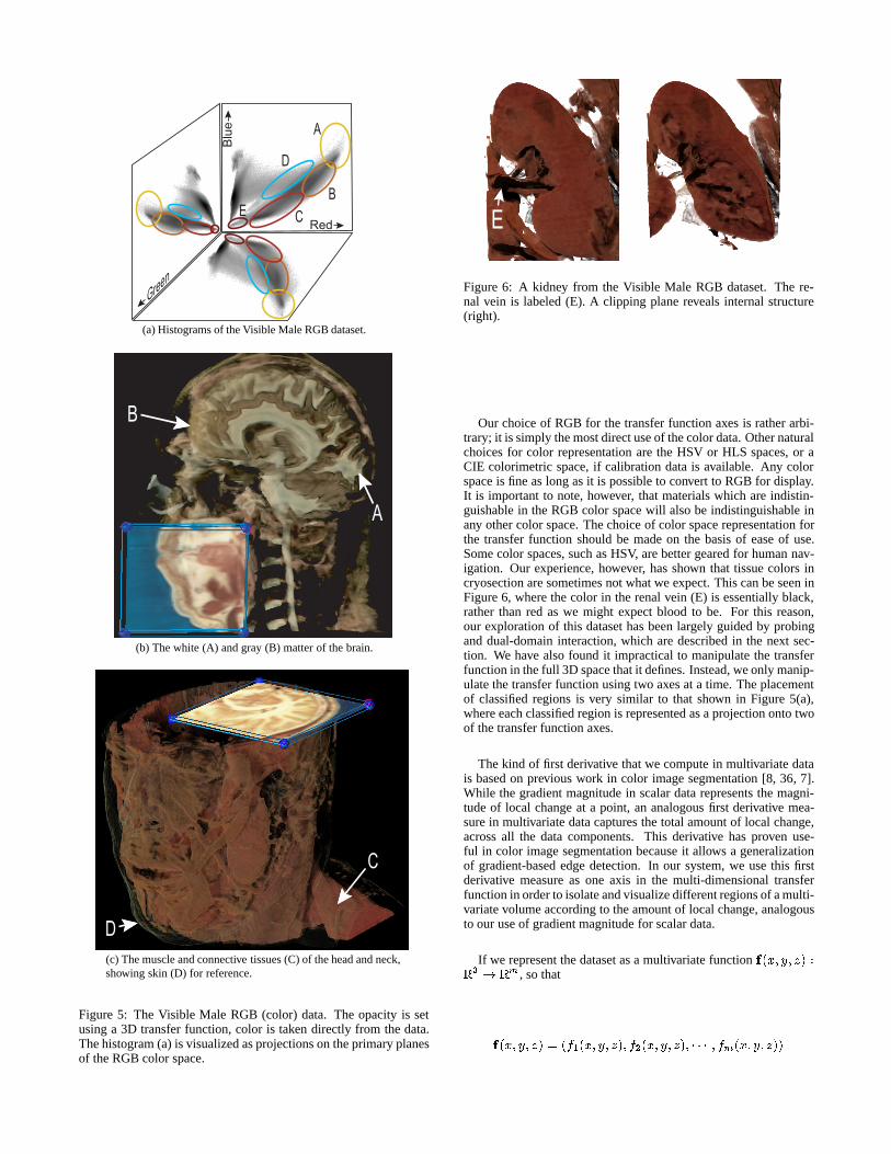
One example of data that benefits from multi-dimensional trans-fer functions is volumetric color data. A number of volumetriccolor datasets are available, such as the Visible Human Project’sRGB data. The process of acquiring color data by cryosection isbecoming common for the investigation of anatomy and histology.In these datasets, the differences in materials are expressed by theirunique spectral signature. A multi-dimensional transfer function isa natural choice for visualizing this type of data. Opacity can be as-signed to different positions in the 3D RGB color space. Figure 5(a)shows a joint histogram of the RGB color data for the Visible Male;regions of this space that correspond to different tissues are identi-fied. Regions (A) and (B) correspond to the fatty tissues of thebrain, white and gray matter, as seen in Figure 5(b). In this visual-ization, the transition between white and grey matter is intentionallyleft out to better emphasize these materials and to demonstrate theexpressivity of the multi-dimensional transfer function. Figure 5(c)shows a visualiation of the color values that represent the musclestructure and connective tissues (C) of the head and neck with theskin surface (D) given a small amount of opacity for context. Inboth of these figures, a slice of the original data is mapped to thesurface of the clipping plane for reference. Figure 6 shows a visu-alization of the kidney from the Visible Male RGB data.

f '

f ''

0

Data Value

+

-

A B C D

E

FG

EF

H

G

H

(a)

(b)

(c) 2D transfer function (d) 3D transfer function

F

G

H

E

Figure 3: Material and boundary identification of the human toothCT with data value and gradient magnitude (f ’), seen in (a), anddata value and second derivative (f”), seen in (b). The back-ground/dentin boundary (F) cannot be adequately captured withdata value and gradient magnitude alone. (c) shows the results ofa 2D transfer function designed to show only the background/detin(F) and dentin/enamel boundaries (G). The background/enamel (H)and dentin/pulp (E) boundaries are erroneously colored. Addingthe second derivative as a third axis to the transfer function dis-ambiguates the boundaries. (d) shows the results of a 3D transferfunction that gives lower opacity to non-zero second derivative val-ues.

x

f(x)f ′(x)f ′′(x)

v1

v2

v3

v4

v5

(a)

f(x)v1 v2 v3 v4 v5

(b)

Figure 4: The behavior of primary data value (f ), gradient magni-tude (f 0), and the second directional derivative (f00) as a functionof position (a) and as a function of data value (b).

Red

Green

Blu

e A

BC

D

E

(a) Histograms of the Visible Male RGB dataset.

A

B

(b) The white (A) and gray (B) matter of the brain.

C

D(c) The muscle and connective tissues (C) of the head and neck,showing skin (D) for reference.

Figure 5: The Visible Male RGB (color) data. The opacity is setusing a 3D transfer function, color is taken directly from the data.The histogram (a) is visualized as projections on the primary planesof the RGB color space.

E

Figure 6: A kidney from the Visible Male RGB dataset. The re-nal vein is labeled (E). A clipping plane reveals internal structure(right).

Our choice of RGB for the transfer function axes is rather arbi-trary; it is simply the most direct use of the color data. Other naturalchoices for color representation are the HSV or HLS spaces, or aCIE colorimetric space, if calibration data is available. Any colorspace is fine as long as it is possible to convert to RGB for display.It is important to note, however, that materials which are indistin-guishable in the RGB color space will also be indistinguishable inany other color space. The choice of color space representation forthe transfer function should be made on the basis of ease of use.Some color spaces, such as HSV, are better geared for human nav-igation. Our experience, however, has shown that tissue colors incryosection are sometimes not what we expect. This can be seen inFigure 6, where the color in the renal vein (E) is essentially black,rather than red as we might expect blood to be. For this reason,our exploration of this dataset has been largely guided by probingand dual-domain interaction, which are described in the next sec-tion. We have also found it impractical to manipulate the transferfunction in the full 3D space that it defines. Instead, we only manip-ulate the transfer function using two axes at a time. The placementof classified regions is very similar to that shown in Figure 5(a),where each classified region is represented as a projection onto twoof the transfer function axes.

The kind of first derivative that we compute in multivariate datais based on previous work in color image segmentation [8, 36, 7].While the gradient magnitude in scalar data represents the magni-tude of local change at a point, an analogous first derivative mea-sure in multivariate data captures the total amount of local change,across all the data components. This derivative has proven use-ful in color image segmentation because it allows a generalizationof gradient-based edge detection. In our system, we use this firstderivative measure as one axis in the multi-dimensional transferfunction in order to isolate and visualize different regions of a multi-variate volume according to the amount of local change, analogousto our use of gradient magnitude for scalar data.

If we represent the dataset as a multivariate function f(x; y; z) :R3 ! R

m , so that

f(x; y; z) = (f1(x; y; z); f2(x; y; z); � � � ; fm(x; y; z))

then the derivative Df is a matrix of first partial derivatives:

Df =

26666666664

@f1@x

@f1@y

@f1@z

@f2@x

@f2@y

@f2@z

...

@fm@x

@fm@y

@fm@z

37777777775

By multiplyingDf with its transpose, we can form a 3�3 tensorG which captures the directional dependence of total change:

G = (Df)TDf (3)

In the context of color edge detection [8, 36, 7], this matrix(specifically, its two-dimensional analog) is used as the basis ofa quadratic function of direction n, which Cumani [7] terms thesquared local contrast in direction n:

S(n) = nTGn

S(n) can be analyzed by finding the principal eigenvector (and as-sociated eigenvalue) of G to determine the direction n of greatestlocal contrast, or fastest change, and the magnitude of that change.Our experience, however, has been that in the context of multi-dimensional transfer functions, it is sufficient (and perhaps prefer-able) to simply take the L2 norm of G, kGk, which is the squareroot of the sum of the squares of the individual matrix components.As the L2 norm is invariant with respect to rotation, this is the sameas the L2 norm of the three eigenvalues of G, motivating our useof kGk as a directionally independent (and rotationally invariant)measure of local change. Other work on volume rendering of colordata has used a non-rotationally invariant measure of G [9]. Sinceit is sometimes the case that the dynamic range of the individualchannels (fi) differ, we normalize the ranges of each channel’s datavalue to be between zero and one. This allows each channel to havean equal contribution in the derivative calculation.

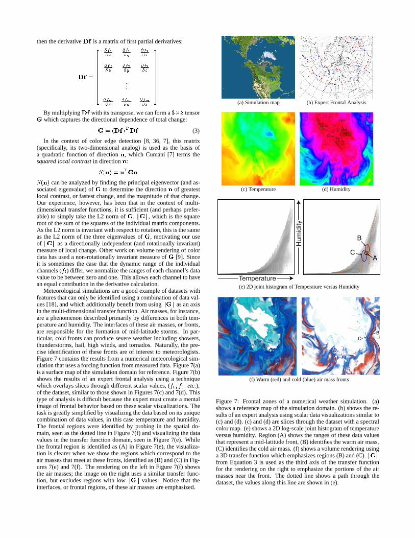
Meteorological simulations are a good example of datasets withfeatures that can only be identified using a combination of data val-ues [18], and which additionally benefit from using kGk as an axisin the multi-dimensional transfer function. Air masses, for instance,are a phenomenon described primarily by differences in both tem-perature and humidity. The interfaces of these air masses, or fronts,are responsible for the formation of mid-latitude storms. In par-ticular, cold fronts can produce severe weather including showers,thunderstorms, hail, high winds, and tornados. Naturally, the pre-cise identification of these fronts are of interest to meteorologists.Figure 7 contains the results from a numerical meteorological sim-ulation that uses a forcing function from measured data. Figure 7(a)is a surface map of the simulation domain for reference. Figure 7(b)shows the results of an expert frontal analysis using a techniquewhich overlays slices through different scalar values, (f1; f2; etc.),of the dataset, similar to those shown in Figures 7(c) and 7(d). Thistype of analysis is difficult because the expert must create a mentalimage of frontal behavior based on these scalar visualizations. Thetask is greatly simplified by visualizing the data based on its uniquecombination of data values, in this case temperature and humidity.The frontal regions were identified by probing in the spatial do-main, seen as the dotted line in Figure 7(f) and visualizing the datavalues in the transfer function domain, seen in Figure 7(e). Whilethe frontal region is identified as (A) in Figure 7(e), the visualiza-tion is clearer when we show the regions which correspond to theair masses that meet at these fronts, identified as (B) and (C) in Fig-ures 7(e) and 7(f). The rendering on the left in Figure 7(f) showsthe air masses; the image on the right uses a similar transfer func-tion, but excludes regions with low kGk values. Notice that theinterfaces, or frontal regions, of these air masses are emphasized.

(a) Simulation map (b) Expert Frontal Analysis

(c) Temperature (d) Humidity

Temperature

Hum

idity

A

B

C

(e) 2D joint histogram of Temperature versus Humidity

CB

(f) Warm (red) and cold (blue) air mass fronts

Figure 7: Frontal zones of a numerical weather simulation. (a)shows a reference map of the simulation domain. (b) shows the re-sults of an expert analysis using scalar data visualizations similar to(c) and (d). (c) and (d) are slices through the dataset with a spectralcolor map. (e) shows a 2D log-scale joint histogram of temperatureversus humidity. Region (A) shows the ranges of these data valuesthat represent a mid-latitude front, (B) identifies the warm air mass,(C) identifies the cold air mass. (f) shows a volume rendering usinga 3D transfer function which emphasizes regions (B) and (C). kGkfrom Equation 3 is used as the third axis of the transfer functionfor the rendering on the right to emphasize the portions of the airmasses near the front. The dotted line shows a path through thedataset, the values along this line are shown in (e).

Data Probe

Clipping Plane

LightWidget

Transfer Function

Classification Widgets

Re-projected VoxelQueried ValueQueried ValueQueried Value

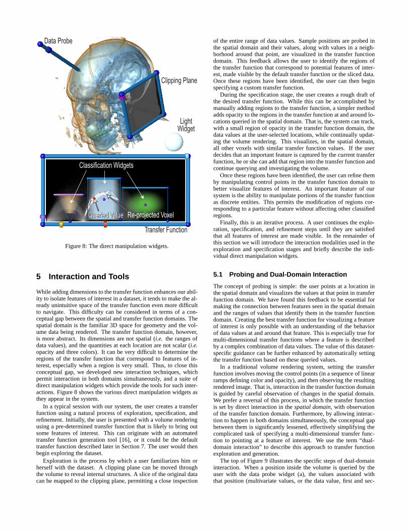
Figure 8: The direct manipulation widgets.

5 Interaction and Tools

While adding dimensions to the transfer function enhances our abil-ity to isolate features of interest in a dataset, it tends to make the al-ready unintuitive space of the transfer function even more difficultto navigate. This difficulty can be considered in terms of a con-ceptual gap between the spatial and transfer function domains. Thespatial domain is the familiar 3D space for geometry and the vol-ume data being rendered. The transfer function domain, however,is more abstract. Its dimensions are not spatial (i.e. the ranges ofdata values), and the quantities at each location are not scalar (i.e.opacity and three colors). It can be very difficult to determine theregions of the transfer function that correspond to features of in-terest, especially when a region is very small. Thus, to close thisconceptual gap, we developed new interaction techniques, whichpermit interaction in both domains simultaneously, and a suite ofdirect manipulation widgets which provide the tools for such inter-actions. Figure 8 shows the various direct manipulation widgets asthey appear in the system.

In a typical session with our system, the user creates a transferfunction using a natural process of exploration, specification, andrefinement. Initially, the user is presented with a volume renderingusing a pre-determined transfer function that is likely to bring outsome features of interest. This can originate with an automatedtransfer function generation tool [16], or it could be the defaulttransfer function described later in Section 7. The user would thenbegin exploring the dataset.

Exploration is the process by which a user familiarizes him orherself with the dataset. A clipping plane can be moved throughthe volume to reveal internal structures. A slice of the original datacan be mapped to the clipping plane, permitting a close inspection

of the entire range of data values. Sample positions are probed inthe spatial domain and their values, along with values in a neigh-borhood around that point, are visualized in the transfer functiondomain. This feedback allows the user to identify the regions ofthe transfer function that correspond to potential features of inter-est, made visible by the default transfer function or the sliced data.Once these regions have been identified, the user can then beginspecifying a custom transfer function.

During the specification stage, the user creates a rough draft ofthe desired transfer function. While this can be accomplished bymanually adding regions to the transfer function, a simpler methodadds opacity to the regions in the transfer function at and around lo-cations queried in the spatial domain. That is, the system can track,with a small region of opacity in the transfer function domain, thedata values at the user-selected locations, while continually updat-ing the volume rendering. This visualizes, in the spatial domain,all other voxels with similar transfer function values. If the userdecides that an important feature is captured by the current transferfunction, he or she can add that region into the transfer function andcontinue querying and investigating the volume.

Once these regions have been identified, the user can refine themby manipulating control points in the transfer function domain tobetter visualize features of interest. An important feature of oursystem is the ability to manipulate portions of the transfer functionas discrete entities. This permits the modification of regions cor-responding to a particular feature without affecting other classifiedregions.

Finally, this is an iterative process. A user continues the explo-ration, specification, and refinement steps until they are satisfiedthat all features of interest are made visible. In the remainder ofthis section we will introduce the interaction modalities used in theexploration and specification stages and briefly describe the indi-vidual direct manipulation widgets.

5.1 Probing and Dual-Domain Interaction

The concept of probing is simple: the user points at a location inthe spatial domain and visualizes the values at that point in transferfunction domain. We have found this feedback to be essential formaking the connection between features seen in the spatial domainand the ranges of values that identify them in the transfer functiondomain. Creating the best transfer function for visualizing a featureof interest is only possible with an understanding of the behaviorof data values at and around that feature. This is especially true formulti-dimensional transfer functions where a feature is describedby a complex combination of data values. The value of this dataset-specific guidance can be further enhanced by automatically settingthe transfer function based on these queried values.

In a traditional volume rendering system, setting the transferfunction involves moving the control points (in a sequence of linearramps defining color and opacity), and then observing the resultingrendered image. That is, interaction in the transfer function domainis guided by careful observation of changes in the spatial domain.We prefer a reversal of this process, in which the transfer functionis set by direct interaction in the spatial domain, with observationof the transfer function domain. Furthermore, by allowing interac-tion to happen in both domains simultaneously, the conceptual gapbetween them is significantly lessened, effectively simplifying thecomplicated task of specifying a multi-dimensional transfer func-tion to pointing at a feature of interest. We use the term “dual-domain interaction” to describe this approach to transfer functionexploration and generation.

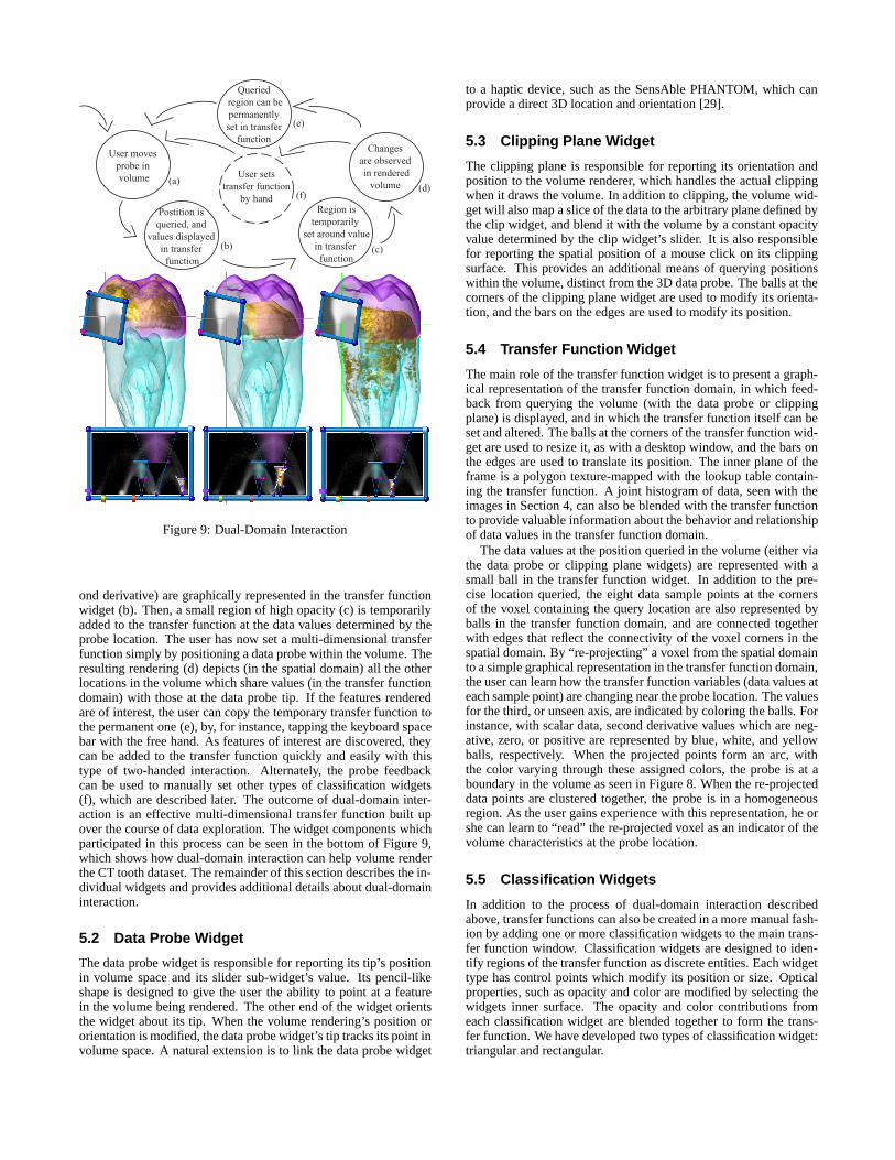
The top of Figure 9 illustrates the specific steps of dual-domaininteraction. When a position inside the volume is queried by theuser with the data probe widget (a), the values associated withthat position (multivariate values, or the data value, first and sec-

User moves probe in volume

Region istemporarily

set around valuein transfer function

Changes are observed in rendered

volume

Postition is queried, and

values displayed in transfer function

Queried region can bepermanently set in transfer

function

User setstransfer function

by hand

(a)

(b) (c)

(d)

(e)

(f)

Figure 9: Dual-Domain Interaction

ond derivative) are graphically represented in the transfer functionwidget (b). Then, a small region of high opacity (c) is temporarilyadded to the transfer function at the data values determined by theprobe location. The user has now set a multi-dimensional transferfunction simply by positioning a data probe within the volume. Theresulting rendering (d) depicts (in the spatial domain) all the otherlocations in the volume which share values (in the transfer functiondomain) with those at the data probe tip. If the features renderedare of interest, the user can copy the temporary transfer function tothe permanent one (e), by, for instance, tapping the keyboard spacebar with the free hand. As features of interest are discovered, theycan be added to the transfer function quickly and easily with thistype of two-handed interaction. Alternately, the probe feedbackcan be used to manually set other types of classification widgets(f), which are described later. The outcome of dual-domain inter-action is an effective multi-dimensional transfer function built upover the course of data exploration. The widget components whichparticipated in this process can be seen in the bottom of Figure 9,which shows how dual-domain interaction can help volume renderthe CT tooth dataset. The remainder of this section describes the in-dividual widgets and provides additional details about dual-domaininteraction.

5.2 Data Probe Widget

The data probe widget is responsible for reporting its tip’s positionin volume space and its slider sub-widget’s value. Its pencil-likeshape is designed to give the user the ability to point at a featurein the volume being rendered. The other end of the widget orientsthe widget about its tip. When the volume rendering’s position ororientation is modified, the data probe widget’s tip tracks its point involume space. A natural extension is to link the data probe widget

to a haptic device, such as the SensAble PHANTOM, which canprovide a direct 3D location and orientation [29].

5.3 Clipping Plane Widget

The clipping plane is responsible for reporting its orientation andposition to the volume renderer, which handles the actual clippingwhen it draws the volume. In addition to clipping, the volume wid-get will also map a slice of the data to the arbitrary plane defined bythe clip widget, and blend it with the volume by a constant opacityvalue determined by the clip widget’s slider. It is also responsiblefor reporting the spatial position of a mouse click on its clippingsurface. This provides an additional means of querying positionswithin the volume, distinct from the 3D data probe. The balls at thecorners of the clipping plane widget are used to modify its orienta-tion, and the bars on the edges are used to modify its position.

5.4 Transfer Function Widget

The main role of the transfer function widget is to present a graph-ical representation of the transfer function domain, in which feed-back from querying the volume (with the data probe or clippingplane) is displayed, and in which the transfer function itself can beset and altered. The balls at the corners of the transfer function wid-get are used to resize it, as with a desktop window, and the bars onthe edges are used to translate its position. The inner plane of theframe is a polygon texture-mapped with the lookup table contain-ing the transfer function. A joint histogram of data, seen with theimages in Section 4, can also be blended with the transfer functionto provide valuable information about the behavior and relationshipof data values in the transfer function domain.

The data values at the position queried in the volume (either viathe data probe or clipping plane widgets) are represented with asmall ball in the transfer function widget. In addition to the pre-cise location queried, the eight data sample points at the cornersof the voxel containing the query location are also represented byballs in the transfer function domain, and are connected togetherwith edges that reflect the connectivity of the voxel corners in thespatial domain. By “re-projecting” a voxel from the spatial domainto a simple graphical representation in the transfer function domain,the user can learn how the transfer function variables (data values ateach sample point) are changing near the probe location. The valuesfor the third, or unseen axis, are indicated by coloring the balls. Forinstance, with scalar data, second derivative values which are neg-ative, zero, or positive are represented by blue, white, and yellowballs, respectively. When the projected points form an arc, withthe color varying through these assigned colors, the probe is at aboundary in the volume as seen in Figure 8. When the re-projecteddata points are clustered together, the probe is in a homogeneousregion. As the user gains experience with this representation, he orshe can learn to “read” the re-projected voxel as an indicator of thevolume characteristics at the probe location.

5.5 Classification Widgets

In addition to the process of dual-domain interaction describedabove, transfer functions can also be created in a more manual fash-ion by adding one or more classification widgets to the main trans-fer function window. Classification widgets are designed to iden-tify regions of the transfer function as discrete entities. Each widgettype has control points which modify its position or size. Opticalproperties, such as opacity and color are modified by selecting thewidgets inner surface. The opacity and color contributions fromeach classification widget are blended together to form the trans-fer function. We have developed two types of classification widget:triangular and rectangular.

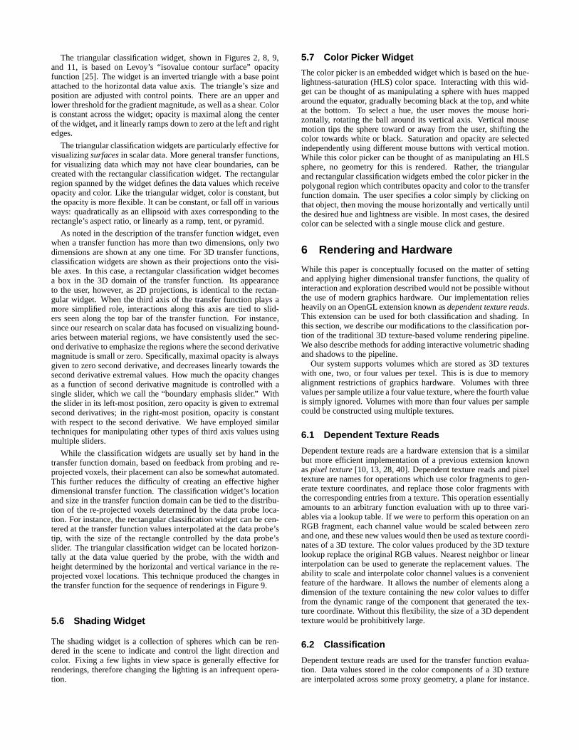
The triangular classification widget, shown in Figures 2, 8, 9,and 11, is based on Levoy’s “isovalue contour surface” opacityfunction [25]. The widget is an inverted triangle with a base pointattached to the horizontal data value axis. The triangle’s size andposition are adjusted with control points. There are an upper andlower threshold for the gradient magnitude, as well as a shear. Coloris constant across the widget; opacity is maximal along the centerof the widget, and it linearly ramps down to zero at the left and rightedges.

The triangular classification widgets are particularly effective forvisualizing surfaces in scalar data. More general transfer functions,for visualizing data which may not have clear boundaries, can becreated with the rectangular classification widget. The rectangularregion spanned by the widget defines the data values which receiveopacity and color. Like the triangular widget, color is constant, butthe opacity is more flexible. It can be constant, or fall off in variousways: quadratically as an ellipsoid with axes corresponding to therectangle’s aspect ratio, or linearly as a ramp, tent, or pyramid.

As noted in the description of the transfer function widget, evenwhen a transfer function has more than two dimensions, only twodimensions are shown at any one time. For 3D transfer functions,classification widgets are shown as their projections onto the visi-ble axes. In this case, a rectangular classification widget becomesa box in the 3D domain of the transfer function. Its appearanceto the user, however, as 2D projections, is identical to the rectan-gular widget. When the third axis of the transfer function plays amore simplified role, interactions along this axis are tied to slid-ers seen along the top bar of the transfer function. For instance,since our research on scalar data has focused on visualizing bound-aries between material regions, we have consistently used the sec-ond derivative to emphasize the regions where the second derivativemagnitude is small or zero. Specifically, maximal opacity is alwaysgiven to zero second derivative, and decreases linearly towards thesecond derivative extremal values. How much the opacity changesas a function of second derivative magnitude is controlled with asingle slider, which we call the “boundary emphasis slider.” Withthe slider in its left-most position, zero opacity is given to extremalsecond derivatives; in the right-most position, opacity is constantwith respect to the second derivative. We have employed similartechniques for manipulating other types of third axis values usingmultiple sliders.

While the classification widgets are usually set by hand in thetransfer function domain, based on feedback from probing and re-projected voxels, their placement can also be somewhat automated.This further reduces the difficulty of creating an effective higherdimensional transfer function. The classification widget’s locationand size in the transfer function domain can be tied to the distribu-tion of the re-projected voxels determined by the data probe loca-tion. For instance, the rectangular classification widget can be cen-tered at the transfer function values interpolated at the data probe’stip, with the size of the rectangle controlled by the data probe’sslider. The triangular classification widget can be located horizon-tally at the data value queried by the probe, with the width andheight determined by the horizontal and vertical variance in the re-projected voxel locations. This technique produced the changes inthe transfer function for the sequence of renderings in Figure 9.

5.6 Shading Widget

The shading widget is a collection of spheres which can be ren-dered in the scene to indicate and control the light direction andcolor. Fixing a few lights in view space is generally effective forrenderings, therefore changing the lighting is an infrequent opera-tion.

5.7 Color Picker Widget

The color picker is an embedded widget which is based on the hue-lightness-saturation (HLS) color space. Interacting with this wid-get can be thought of as manipulating a sphere with hues mappedaround the equator, gradually becoming black at the top, and whiteat the bottom. To select a hue, the user moves the mouse hori-zontally, rotating the ball around its vertical axis. Vertical mousemotion tips the sphere toward or away from the user, shifting thecolor towards white or black. Saturation and opacity are selectedindependently using different mouse buttons with vertical motion.While this color picker can be thought of as manipulating an HLSsphere, no geometry for this is rendered. Rather, the triangularand rectangular classification widgets embed the color picker in thepolygonal region which contributes opacity and color to the transferfunction domain. The user specifies a color simply by clicking onthat object, then moving the mouse horizontally and vertically untilthe desired hue and lightness are visible. In most cases, the desiredcolor can be selected with a single mouse click and gesture.

6 Rendering and Hardware

While this paper is conceptually focused on the matter of settingand applying higher dimensional transfer functions, the quality ofinteraction and exploration described would not be possible withoutthe use of modern graphics hardware. Our implementation reliesheavily on an OpenGL extension known as dependent texture reads.This extension can be used for both classification and shading. Inthis section, we describe our modifications to the classification por-tion of the traditional 3D texture-based volume rendering pipeline.We also describe methods for adding interactive volumetric shadingand shadows to the pipeline.

Our system supports volumes which are stored as 3D textureswith one, two, or four values per texel. This is is due to memoryalignment restrictions of graphics hardware. Volumes with threevalues per sample utilize a four value texture, where the fourth valueis simply ignored. Volumes with more than four values per samplecould be constructed using multiple textures.

6.1 Dependent Texture Reads

Dependent texture reads are a hardware extension that is a similarbut more efficient implementation of a previous extension knownas pixel texture [10, 13, 28, 40]. Dependent texture reads and pixeltexture are names for operations which use color fragments to gen-erate texture coordinates, and replace those color fragments withthe corresponding entries from a texture. This operation essentiallyamounts to an arbitrary function evaluation with up to three vari-ables via a lookup table. If we were to perform this operation on anRGB fragment, each channel value would be scaled between zeroand one, and these new values would then be used as texture coordi-nates of a 3D texture. The color values produced by the 3D texturelookup replace the original RGB values. Nearest neighbor or linearinterpolation can be used to generate the replacement values. Theability to scale and interpolate color channel values is a convenientfeature of the hardware. It allows the number of elements along adimension of the texture containing the new color values to differfrom the dynamic range of the component that generated the tex-ture coordinate. Without this flexibility, the size of a 3D dependenttexture would be prohibitively large.

6.2 Classification

Dependent texture reads are used for the transfer function evalua-tion. Data values stored in the color components of a 3D textureare interpolated across some proxy geometry, a plane for instance.

These values are then converted to texture coordinates and usedto acquire the color and alpha values in the transfer function tex-ture per-pixel in screen space. For eight bit data, an ideal transferfunction texture would have 256 color and alpha values along eachaxis. For 3D transfer functions, however, the transfer function tex-ture would then be 2563 � 4 bytes. Besides the enormous memoryrequirements of such a texture, the size also affects how fast theclassification widgets can be rasterized, thus affecting the interac-tivity of transfer function updates. We therefore limit the numberof elements along an axis of a 3D transfer function based on its im-portance. For instance, with scalar data, the primary data value isthe most important, the gradient magnitude is secondary, and thesecond derivative serves an even more tertiary role. For this type ofmulti-dimensional transfer function, we commonly use a 3D trans-fer function texture with dimensions 256� 128� 8 for data value,gradient magnitude, and second derivative respectively. 3D transferfunctions can also be composed separably as a 2D and 1D trans-fer function. This means that the total size of the transfer functionis 2562 + 256. The tradeoff, however, is in expressivity. We canno longer specify a transfer function based on the unique combina-tion of all three data values. Separable transfer functions are stillquite powerful. Applying the second derivative as a separable 1Dportion of the transfer functions is quite effective for visualizingboundaries between materials. With the separable 3D transfer func-tion for scalar volumes, there is only one boundary emphasis sliderwhich affects all classification widgets as opposed to the generalcase where each classification widget has its own boundary empha-sis slider. We have employed a similar approach for multi-variatedata visualization. The meteorological example used a separable3D transfer function. Temperature and humidity were classified us-ing a 2D transfer function and the multi-derivative of these valueswas classified using a 1D transfer function. Since our specific goalwas to show only regions with high values of kGk, we only neededtwo sliders to specify the beginning and ending points of a linearramp along this axis of the transfer function.

6.3 Surface Shading

Shading is a fundamental component of volume rendering becauseit is a natural and efficient way to express information about theshape of structures in the volume. However, much previous workwith texture-memory based volume rendering lacks shading. Manymodern graphics hardware platforms support multi-texture and anumber of user defined operations for blending these textures per-pixel. These operations, which we will refer to as fragment shading,can be leveraged to compute a surface shading model.

The technique originally proposed by Rezk-Salama et al. [6] isan efficient way to compute the Blinn-Phong shading model ona per-pixel basis for volumes. This approach, however, can suf-fer from artifacts caused by denormalization during interpolation.While future generations of graphics hardware should support thesquare root operation needed to renormalize on a per-pixel basis,we can utilize cube map dependent texture reads to evaluate theshading model. This type of dependent texture read allows an RGBcolor component to be treated as a vector and used as the texture co-ordinates for a cube map. Conceptually, a cube map can be thoughtof as a collection of six textures that make up the faces of a cubecentered about the origin. Texels are accessed with a 3D texture co-ordinate (s,t,r) representing a direction vector. The accessed texelis the point corresponding to the intersection of a line through theorigin in the direction of (s,t,r) and a cube face. The color values atthis position represent incoming diffuse radiance if the vector (s,t,r)is a surface normal or specular radiance if (s,t,r) is a reflection vec-tor. The advantages of using a cube map dependent texture read isthat the vector (s,t,r) does not need to be normalized, and the cubemap can encode an arbitrary number of lights or a full environment

map. This approach, however, comes at the cost of reduced perfor-mance. A per-pixel cube map evaluation can be as much as threetimes slower than evaluating the dot products for a limited numberof light sources in the fragment shader stage.

Surface based shading methods are well suited for visualizing theboundaries between materials. However, since the surface normalis approximated by the normalized gradient of a scalar field, thesemethods are not robust for shading homogeneous regions, wherethe gradient magnitude is very low or zero and its measurement issensitive to noise. Gradient based surface shading is also unsuitablefor shading volume renderings of multivariate fields. While we canassign the direction of greatest change for a point in a multivariatefield to the eigenvector (e1) corresponding to the largest eigenvalue(�1) of the tensorG from Equation 3, e1 is only a valid representa-tion of orientation, not the absolute direction. This means that thesign of e1 can flip in neighboring regions even though their orienta-tions may not differ. Therefore, the vector e1 does not interpolate,making it a poor choice of surface normal. Furthermore, this orien-tation may not even correspond to the surface normal of a classifiedregion in a multivariate field.

6.4 Shadows

Shadows provide important visual queues relating to the depth andplacement of objects in a scene. Since the computation of shad-ows does not depend on a surface normal, they provide a robustmethod for shading homogeneous regions and multivariate vol-umes. Adding shadows to the volume lighting model means thatlight gets attenuated through the volume before being reflected backto the eye.

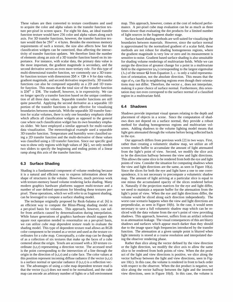
Our approach differs from previous work [2] in two ways. First,rather than creating a volumetric shadow map, we utilize an offscreen render buffer to accumulate the amount of light attenuatedfrom the light’s point of view. Second, we modify the slice axisto be the direction halfway between the view and light directions.This allows the same slice to be rendered from both the eye and lightpoints of view. Consider the situation for computing shadows whenthe view and light directions are the same, as seen in Figure 10(a).Since the slices for both the eye and light have a one to one corre-spondence, it is not necessary to precompute a volumetric shadowmap. The amount of light arriving at a particular slice is equal toone minus the accumulated opacity of the slices rendered beforeit. Naturally if the projection matrices for the eye and light differ,we need to maintain a separate buffer for the attenuation from thelight’s point of view. When the eye and light directions differ, thevolume would be sliced along each direction independently. Theworst case scenario happens when the view and light directions areperpendicular, as seen in Figure 10(b). In the case, it would seemnecessary to save a full volumetric shadow map which can be re-sliced with the data volume from the eye’s point of view providingshadows. This approach, however, suffers from an artifact referredto as attenuation leakage. The visual consequences of this are blurryshadows and surfaces which appear much darker than they shoulddue to the image space high frequencies introduced by the transferfunction. The attenuation at a given sample point is blurred whenlight intensity is stored at a coarse resolution and interpolated dur-ing the observer rendering phase.

Rather than slice along the vector defined by the view directionor the light direction, we modify the slice axis to allow the sameslice to be rendered from both points of view. When the dot prod-uct of the light and view directions is positive, we slice along thevector halfway between the light and view directions, seen in Fig-ure 10(c). In this case, the volume is rendered in front to back orderwith respect to the observer. When the dot product is negative, weslice along the vector halfway between the light and the invertedview directions, seen in Figure 10(d). In this case, the volume is

v v -v

l lss

θ

12−θ

vl

v

l

(a) (b)

(c) (d)

Figure 10: Modified slice axis for light transport.

rendered in back to front order with respect to the observer. In bothcases the volume is rendered in front to back order with respect tothe light. Care must be taken to insure that the slice spacing alongthe view and light directions are maintained when the light or eyepositions change. If the desired slice spacing along the view direc-tion is dv and the angle between v and l is � then the slice spacingalong the slice direction is

ds = cos(�

2)dv: (4)

This is a multi-pass approach. Each slice is first rendered fromthe observers point of view using the results of the previous passfrom the light’s point of view, which modulates the brightness ofsamples in the current slice. The same slice is then rendered fromlight’s point of view to calculate the intensity of the light arriving atthe next layer.

Since we must keep track of the amount of light attenuated ateach slice, we utilize an off screen render buffer, known as a pixelbuffer. This buffer is initialized to 1 � light intensity. It canalso be initialized using an arbitrary image to create effects such asspotlights. The projection matrix for the light’s point of view neednot be orthographic; a perspective projection matrix can be usedfor point light sources. However, the entire volume must fit in thelight’s view frustum. Light is attenuated by simply accumulatingthe opacity for each sample using the over operator. The resultsare then copied to a texture which is multiplied with the next slicefrom the eye’s point of view before it is blended into the framebuffer. While this copy to texture operation has been highly op-timized on the current generation of graphics hardware, we haveachieved a dramatic increase in performance using a hardware ex-tension known as render to texture. This extension allows us todirectly bind a pixel buffer as a texture, avoiding the unnecessarycopy operation.

This approach has a number of advantages over previous volumeshadow methods. First, attenuation leakage is no longer a concernbecause the computation of the light transport (slicing density) isdecoupled from the resolution of the data volume. Computing lightattenuation in image space allows us to match the sampling fre-quency of the light transport with that of the final volume render-ing. Second, this approach makes far more efficient use of memoryresources than those which require a volumetric shadow map. Onlya single additional 2D buffer is required as opposed to a potentiallylarge 3D volume. One disadvantage of this approach is that due to

the image space sampling, artifacts may appear at shadow bound-aries when the opacity makes a sharp jump from low to high. Thiscan be overcome by using a higher resolution for the light bufferthan for the frame buffer. We have found that 30 to 50 percent ad-ditional resolution is adequate.

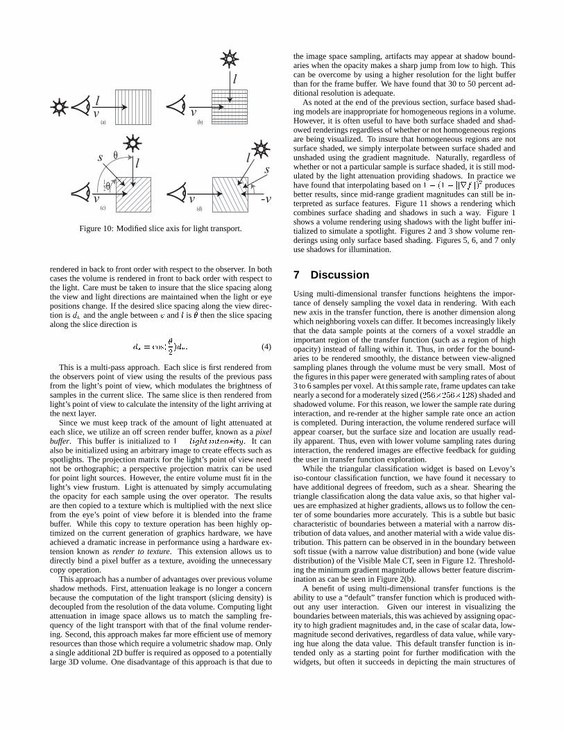
As noted at the end of the previous section, surface based shad-ing models are inappropriate for homogeneous regions in a volume.However, it is often useful to have both surface shaded and shad-owed renderings regardless of whether or not homogeneous regionsare being visualized. To insure that homogeneous regions are notsurface shaded, we simply interpolate between surface shaded andunshaded using the gradient magnitude. Naturally, regardless ofwhether or not a particular sample is surface shaded, it is still mod-ulated by the light attenuation providing shadows. In practice wehave found that interpolating based on 1� (1� krfk)2 producesbetter results, since mid-range gradient magnitudes can still be in-terpreted as surface features. Figure 11 shows a rendering whichcombines surface shading and shadows in such a way. Figure 1shows a volume rendering using shadows with the light buffer ini-tialized to simulate a spotlight. Figures 2 and 3 show volume ren-derings using only surface based shading. Figures 5, 6, and 7 onlyuse shadows for illumination.

7 Discussion

Using multi-dimensional transfer functions heightens the impor-tance of densely sampling the voxel data in rendering. With eachnew axis in the transfer function, there is another dimension alongwhich neighboring voxels can differ. It becomes increasingly likelythat the data sample points at the corners of a voxel straddle animportant region of the transfer function (such as a region of highopacity) instead of falling within it. Thus, in order for the bound-aries to be rendered smoothly, the distance between view-alignedsampling planes through the volume must be very small. Most ofthe figures in this paper were generated with sampling rates of about3 to 6 samples per voxel. At this sample rate, frame updates can takenearly a second for a moderately sized (256�256�128) shaded andshadowed volume. For this reason, we lower the sample rate duringinteraction, and re-render at the higher sample rate once an actionis completed. During interaction, the volume rendered surface willappear coarser, but the surface size and location are usually read-ily apparent. Thus, even with lower volume sampling rates duringinteraction, the rendered images are effective feedback for guidingthe user in transfer function exploration.

While the triangular classification widget is based on Levoy’siso-contour classification function, we have found it necessary tohave additional degrees of freedom, such as a shear. Shearing thetriangle classification along the data value axis, so that higher val-ues are emphasized at higher gradients, allows us to follow the cen-ter of some boundaries more accurately. This is a subtle but basiccharacteristic of boundaries between a material with a narrow dis-tribution of data values, and another material with a wide value dis-tribution. This pattern can be observed in in the boundary betweensoft tissue (with a narrow value distribution) and bone (wide valuedistribution) of the Visible Male CT, seen in Figure 12. Threshold-ing the minimum gradient magnitude allows better feature discrim-ination as can be seen in Figure 2(b).

A benefit of using multi-dimensional transfer functions is theability to use a “default” transfer function which is produced with-out any user interaction. Given our interest in visualizing theboundaries between materials, this was achieved by assigning opac-ity to high gradient magnitudes and, in the case of scalar data, low-magnitude second derivatives, regardless of data value, while vary-ing hue along the data value. This default transfer function is in-tended only as a starting point for further modification with thewidgets, but often it succeeds in depicting the main structures of

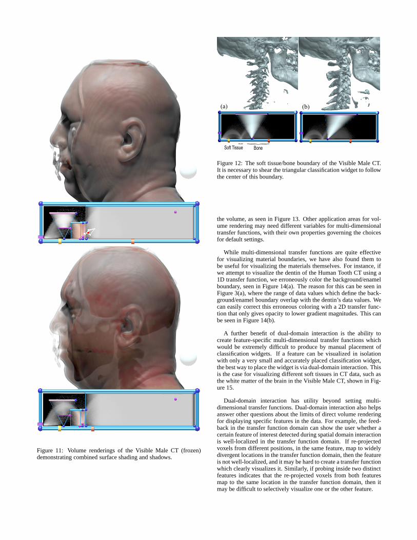
Figure 11: Volume renderings of the Visible Male CT (frozen)demonstrating combined surface shading and shadows.

{ {

Soft Tissue Bone

(a) (b)

Figure 12: The soft tissue/bone boundary of the Visible Male CT.It is necessary to shear the triangular classification widget to followthe center of this boundary.

the volume, as seen in Figure 13. Other application areas for vol-ume rendering may need different variables for multi-dimensionaltransfer functions, with their own properties governing the choicesfor default settings.

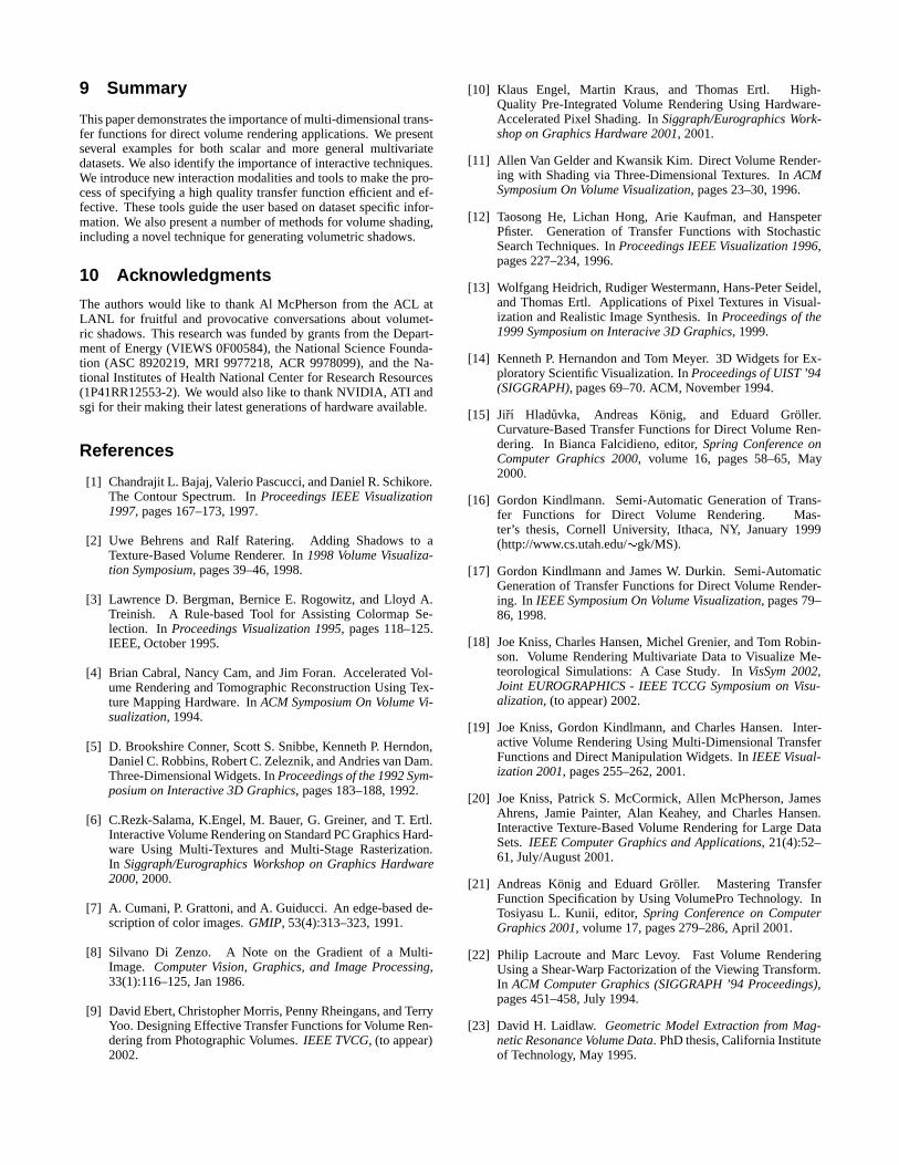
While multi-dimensional transfer functions are quite effectivefor visualizing material boundaries, we have also found them tobe useful for visualizing the materials themselves. For instance, ifwe attempt to visualize the dentin of the Human Tooth CT using a1D transfer function, we erroneously color the background/enamelboundary, seen in Figure 14(a). The reason for this can be seen inFigure 3(a), where the range of data values which define the back-ground/enamel boundary overlap with the dentin’s data values. Wecan easily correct this erroneous coloring with a 2D transfer func-tion that only gives opacity to lower gradient magnitudes. This canbe seen in Figure 14(b).

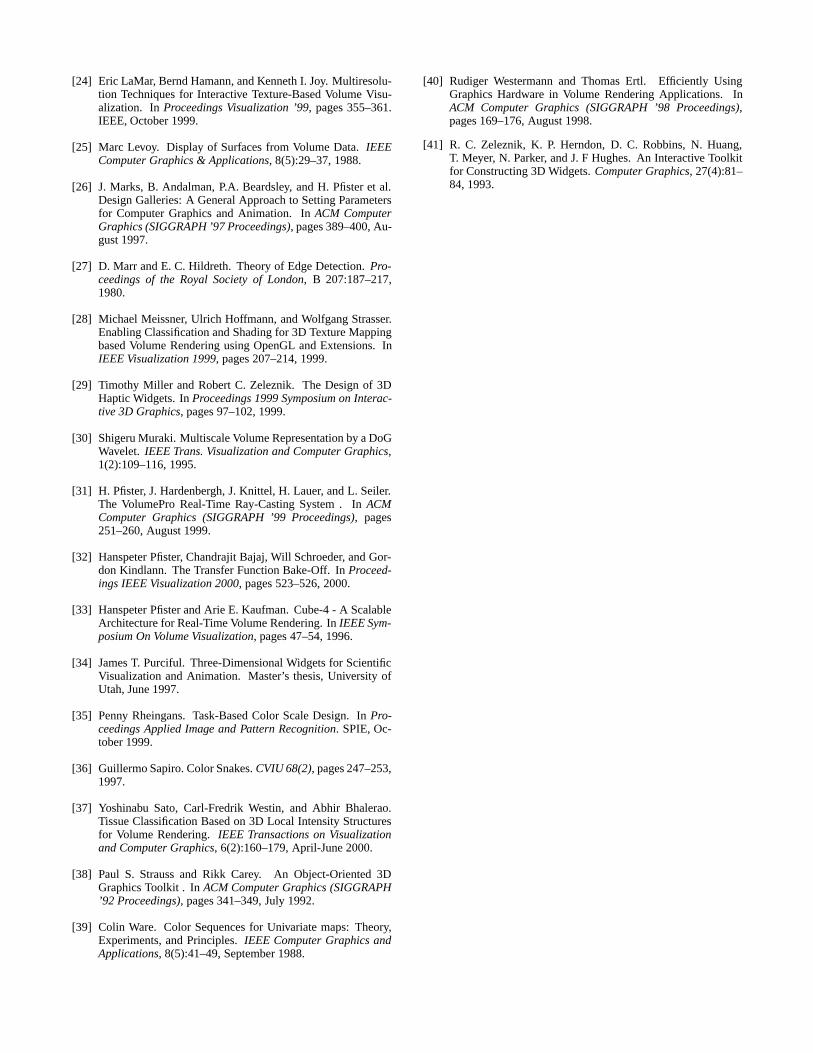
A further benefit of dual-domain interaction is the ability tocreate feature-specific multi-dimensional transfer functions whichwould be extremely difficult to produce by manual placement ofclassification widgets. If a feature can be visualized in isolationwith only a very small and accurately placed classification widget,the best way to place the widget is via dual-domain interaction. Thisis the case for visualizing different soft tissues in CT data, such asthe white matter of the brain in the Visible Male CT, shown in Fig-ure 15.

Dual-domain interaction has utility beyond setting multi-dimensional transfer functions. Dual-domain interaction also helpsanswer other questions about the limits of direct volume renderingfor displaying specific features in the data. For example, the feed-back in the transfer function domain can show the user whether acertain feature of interest detected during spatial domain interactionis well-localized in the transfer function domain. If re-projectedvoxels from different positions, in the same feature, map to widelydivergent locations in the transfer function domain, then the featureis not well-localized, and it may be hard to create a transfer functionwhich clearly visualizes it. Similarly, if probing inside two distinctfeatures indicates that the re-projected voxels from both featuresmap to the same location in the transfer function domain, then itmay be difficult to selectively visualize one or the other feature.

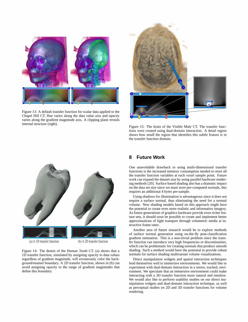
Figure 13: A default transfer function for scalar data applied to theChapel Hill CT. Hue varies along the data value axis and opacityvaries along the gradient magnitude axis. A clipping plane revealsinternal structure (right).

(a) A 1D transfer function (b) A 2D transfer function

Figure 14: The dentin of the Human Tooth CT. (a) shows that a1D transfer function, simulated by assigning opacity to data valuesregardless of gradient magnitude, will erroneously color the back-ground/enamel boundary. A 2D transfer function, shown in (b) canavoid assigning opacity to the range of gradient magnitudes thatdefine this boundary.

Figure 15: The brain of the Visible Male CT. The transfer func-tions were created using dual-domain interaction. A detail regionshows how small the region that identifies this subtle feature is inthe transfer function domain.

8 Future Work

One unavoidable drawback to using multi-dimensional transferfunctions is the increased memory consumption needed to store allthe transfer function variables at each voxel sample point. Futurework can expand the dataset size by using parallel hardware render-ing methods [20]. Surface based shading also has a dramatic impacton the data set size since we must store pre-computed normals, thisrequires an additional 4 bytes per-sample.

Using shadows for illumination is advantageous since it does notrequire a surface normal, thus eliminating the need for a normalvolume. New shading models based on this approach might havethe potential to create even more realistic and informative imagery.As future generations of graphics hardware provide even richer fea-ture sets, it should soon be possible to create and implement betterapproximations of light transport through volumetric media at in-teractive frame rates.

Another area of future research would be to explore methodsof surface normal generation using on-the-fly post-classificationgradient estimation. This is a non-trivial problem since the trans-fer function can introduce very high frequencies or discontinuities,which can be problematic for creating normals that produce smoothshading. Such a method would have the potential to provide robustnormals for surface shading multivariate volume visualizations.

Direct manipulation widgets and spatial interaction techniqueslend themselves well to immersive environments. We would like toexperiment with dual-domain interaction in a stereo, tracked, envi-ronment. We speculate that an immersive environment could makeinteracting with a 3D transfer function more natural and intuitive.We would also like to perform usability studies on our direct ma-nipulation widgets and dual-domain interaction technique, as wellas perceptual studies on 2D and 3D transfer functions for volumerendering.

9 Summary

This paper demonstrates the importance of multi-dimensional trans-fer functions for direct volume rendering applications. We presentseveral examples for both scalar and more general multivariatedatasets. We also identify the importance of interactive techniques.We introduce new interaction modalities and tools to make the pro-cess of specifying a high quality transfer function efficient and ef-fective. These tools guide the user based on dataset specific infor-mation. We also present a number of methods for volume shading,including a novel technique for generating volumetric shadows.

10 Acknowledgments

The authors would like to thank Al McPherson from the ACL atLANL for fruitful and provocative conversations about volumet-ric shadows. This research was funded by grants from the Depart-ment of Energy (VIEWS 0F00584), the National Science Founda-tion (ASC 8920219, MRI 9977218, ACR 9978099), and the Na-tional Institutes of Health National Center for Research Resources(1P41RR12553-2). We would also like to thank NVIDIA, ATI andsgi for their making their latest generations of hardware available.

References

[1] Chandrajit L. Bajaj, Valerio Pascucci, and Daniel R. Schikore.The Contour Spectrum. In Proceedings IEEE Visualization1997, pages 167–173, 1997.

[2] Uwe Behrens and Ralf Ratering. Adding Shadows to aTexture-Based Volume Renderer. In 1998 Volume Visualiza-tion Symposium, pages 39–46, 1998.

[3] Lawrence D. Bergman, Bernice E. Rogowitz, and Lloyd A.Treinish. A Rule-based Tool for Assisting Colormap Se-lection. In Proceedings Visualization 1995, pages 118–125.IEEE, October 1995.

[4] Brian Cabral, Nancy Cam, and Jim Foran. Accelerated Vol-ume Rendering and Tomographic Reconstruction Using Tex-ture Mapping Hardware. In ACM Symposium On Volume Vi-sualization, 1994.

[5] D. Brookshire Conner, Scott S. Snibbe, Kenneth P. Herndon,Daniel C. Robbins, Robert C. Zeleznik, and Andries van Dam.Three-Dimensional Widgets. In Proceedings of the 1992 Sym-posium on Interactive 3D Graphics, pages 183–188, 1992.

[6] C.Rezk-Salama, K.Engel, M. Bauer, G. Greiner, and T. Ertl.Interactive Volume Rendering on Standard PC Graphics Hard-ware Using Multi-Textures and Multi-Stage Rasterization.In Siggraph/Eurographics Workshop on Graphics Hardware2000, 2000.

[7] A. Cumani, P. Grattoni, and A. Guiducci. An edge-based de-scription of color images. GMIP, 53(4):313–323, 1991.

[8] Silvano Di Zenzo. A Note on the Gradient of a Multi-Image. Computer Vision, Graphics, and Image Processing,33(1):116–125, Jan 1986.

[9] David Ebert, Christopher Morris, Penny Rheingans, and TerryYoo. Designing Effective Transfer Functions for Volume Ren-dering from Photographic Volumes. IEEE TVCG, (to appear)2002.

[10] Klaus Engel, Martin Kraus, and Thomas Ertl. High-Quality Pre-Integrated Volume Rendering Using Hardware-Accelerated Pixel Shading. In Siggraph/Eurographics Work-shop on Graphics Hardware 2001, 2001.

[11] Allen Van Gelder and Kwansik Kim. Direct Volume Render-ing with Shading via Three-Dimensional Textures. In ACMSymposium On Volume Visualization, pages 23–30, 1996.

[12] Taosong He, Lichan Hong, Arie Kaufman, and HanspeterPfister. Generation of Transfer Functions with StochasticSearch Techniques. In Proceedings IEEE Visualization 1996,pages 227–234, 1996.

[13] Wolfgang Heidrich, Rudiger Westermann, Hans-Peter Seidel,and Thomas Ertl. Applications of Pixel Textures in Visual-ization and Realistic Image Synthesis. In Proceedings of the1999 Symposium on Interacive 3D Graphics, 1999.

[14] Kenneth P. Hernandon and Tom Meyer. 3D Widgets for Ex-ploratory Scientific Visualization. In Proceedings of UIST ’94(SIGGRAPH), pages 69–70. ACM, November 1994.

[15] Jirı Hladuvka, Andreas Konig, and Eduard Groller.Curvature-Based Transfer Functions for Direct Volume Ren-dering. In Bianca Falcidieno, editor, Spring Conference onComputer Graphics 2000, volume 16, pages 58–65, May2000.

[16] Gordon Kindlmann. Semi-Automatic Generation of Trans-fer Functions for Direct Volume Rendering. Mas-ter’s thesis, Cornell University, Ithaca, NY, January 1999(http://www.cs.utah.edu/�gk/MS).

[17] Gordon Kindlmann and James W. Durkin. Semi-AutomaticGeneration of Transfer Functions for Direct Volume Render-ing. In IEEE Symposium On Volume Visualization, pages 79–86, 1998.

[18] Joe Kniss, Charles Hansen, Michel Grenier, and Tom Robin-son. Volume Rendering Multivariate Data to Visualize Me-teorological Simulations: A Case Study. In VisSym 2002,Joint EUROGRAPHICS - IEEE TCCG Symposium on Visu-alization, (to appear) 2002.

[19] Joe Kniss, Gordon Kindlmann, and Charles Hansen. Inter-active Volume Rendering Using Multi-Dimensional TransferFunctions and Direct Manipulation Widgets. In IEEE Visual-ization 2001, pages 255–262, 2001.

[20] Joe Kniss, Patrick S. McCormick, Allen McPherson, JamesAhrens, Jamie Painter, Alan Keahey, and Charles Hansen.Interactive Texture-Based Volume Rendering for Large DataSets. IEEE Computer Graphics and Applications, 21(4):52–61, July/August 2001.

[21] Andreas Konig and Eduard Groller. Mastering TransferFunction Specification by Using VolumePro Technology. InTosiyasu L. Kunii, editor, Spring Conference on ComputerGraphics 2001, volume 17, pages 279–286, April 2001.

[22] Philip Lacroute and Marc Levoy. Fast Volume RenderingUsing a Shear-Warp Factorization of the Viewing Transform.In ACM Computer Graphics (SIGGRAPH ’94 Proceedings),pages 451–458, July 1994.

[23] David H. Laidlaw. Geometric Model Extraction from Mag-netic Resonance Volume Data. PhD thesis, California Instituteof Technology, May 1995.

[24] Eric LaMar, Bernd Hamann, and Kenneth I. Joy. Multiresolu-tion Techniques for Interactive Texture-Based Volume Visu-alization. In Proceedings Visualization ’99, pages 355–361.IEEE, October 1999.

[25] Marc Levoy. Display of Surfaces from Volume Data. IEEEComputer Graphics & Applications, 8(5):29–37, 1988.

[26] J. Marks, B. Andalman, P.A. Beardsley, and H. Pfister et al.Design Galleries: A General Approach to Setting Parametersfor Computer Graphics and Animation. In ACM ComputerGraphics (SIGGRAPH ’97 Proceedings), pages 389–400, Au-gust 1997.

[27] D. Marr and E. C. Hildreth. Theory of Edge Detection. Pro-ceedings of the Royal Society of London, B 207:187–217,1980.

[28] Michael Meissner, Ulrich Hoffmann, and Wolfgang Strasser.Enabling Classification and Shading for 3D Texture Mappingbased Volume Rendering using OpenGL and Extensions. InIEEE Visualization 1999, pages 207–214, 1999.

[29] Timothy Miller and Robert C. Zeleznik. The Design of 3DHaptic Widgets. In Proceedings 1999 Symposium on Interac-tive 3D Graphics, pages 97–102, 1999.

[30] Shigeru Muraki. Multiscale Volume Representation by a DoGWavelet. IEEE Trans. Visualization and Computer Graphics,1(2):109–116, 1995.

[31] H. Pfister, J. Hardenbergh, J. Knittel, H. Lauer, and L. Seiler.The VolumePro Real-Time Ray-Casting System . In ACMComputer Graphics (SIGGRAPH ’99 Proceedings), pages251–260, August 1999.

[32] Hanspeter Pfister, Chandrajit Bajaj, Will Schroeder, and Gor-don Kindlann. The Transfer Function Bake-Off. In Proceed-ings IEEE Visualization 2000, pages 523–526, 2000.

[33] Hanspeter Pfister and Arie E. Kaufman. Cube-4 - A ScalableArchitecture for Real-Time Volume Rendering. In IEEE Sym-posium On Volume Visualization, pages 47–54, 1996.

[34] James T. Purciful. Three-Dimensional Widgets for ScientificVisualization and Animation. Master’s thesis, University ofUtah, June 1997.

[35] Penny Rheingans. Task-Based Color Scale Design. In Pro-ceedings Applied Image and Pattern Recognition. SPIE, Oc-tober 1999.

[36] Guillermo Sapiro. Color Snakes. CVIU 68(2), pages 247–253,1997.

[37] Yoshinabu Sato, Carl-Fredrik Westin, and Abhir Bhalerao.Tissue Classification Based on 3D Local Intensity Structuresfor Volume Rendering. IEEE Transactions on Visualizationand Computer Graphics, 6(2):160–179, April-June 2000.

[38] Paul S. Strauss and Rikk Carey. An Object-Oriented 3DGraphics Toolkit . In ACM Computer Graphics (SIGGRAPH’92 Proceedings), pages 341–349, July 1992.

[39] Colin Ware. Color Sequences for Univariate maps: Theory,Experiments, and Principles. IEEE Computer Graphics andApplications, 8(5):41–49, September 1988.

[40] Rudiger Westermann and Thomas Ertl. Efficiently UsingGraphics Hardware in Volume Rendering Applications. InACM Computer Graphics (SIGGRAPH ’98 Proceedings),pages 169–176, August 1998.

[41] R. C. Zeleznik, K. P. Herndon, D. C. Robbins, N. Huang,T. Meyer, N. Parker, and J. F Hughes. An Interactive Toolkitfor Constructing 3D Widgets. Computer Graphics, 27(4):81–84, 1993.