Multifractal modelling and simulation of rain fields

$Page 1: Multifractal modelling and simulation of rain fields$
Multifractal modelling and simulation of rain fields exhibiting spatial heterogeneity

695

Hydrology and Earth System Sciences, 6(4), 695–708 (2002) © EGS

Multifractal modelling and simulation of rain fields exhibitingspatial heterogeneityAssela Pathirana1 and Srikantha Herath2

1Faculty of Science and Engineering, Chuo University, Kasuga, Bunkyo-ku, Tokyo, Japan2Institute of Industrial Science, University of Tokyo, Komaba, Meguro, Tokyo, Japan

Email for corresponding author: [email protected]

AbstractSpatial multifractals are statistically homogeneous random fields. While being useful to model geophysical fields exhibiting a high degree ofvariability and discontinuity and including rainfall, they ignore the spatial trends embedded in the variability that are evident from largetemporal aggregation of spatial fields. The modelling of rain fields using multifractals causes the information related to spatial heterogeneity,immensely important at some spatial scales, to be lost in the modelling process. A simple method to avoid this loss of the heterogeneityinformation is proposed. Instead of modelling rain fields directly as multifractals, a derived field M is modelled; this is the product offiltering observed rainfall snapshots with spatial heterogeneity as indicated by long term accumulations of rain fields. The validity of consideringthe field M as multifractal is investigated empirically. The applicability of the proposed method is demonstrated using a discrete cascademodel on gauge-calibrated radar rainfall of central Japan at a daily scale. Important parameters of spatial rainfall, like the distribution of wetareas, spatial autocorrelation and rainfall intensity distributions at different geographic locations with different amounts of average rainfall,were faithfully reproduced by the proposed method.

Keywords: spatial rainfall, downscaling, multifractals

IntroductionInvestigations of weather and climatic systems at a globalscale have become a prime area of research for a number ofreasons among which the concern about global climaticchange is a main one. In addition to an increased scientificunderstanding of atmospheric processes, many usefulforecasting products have become available. These includeregional and global climatic models, which predict short-term weather patterns and longer term trends in climate at acoarser scale. Hydrologists are often involved in solvingproblems that concern much smaller scales than those ofglobal or regional models. Many attempts have been madein the past to bridge the gap between the regional and thecatchment scale. Deterministic resolving of spatial rainfall at sub-grid scalecannot be achieved with only the information provided bylarge-scale forcing. The simplest scheme to distribute rainfallat sub-grid scale would be to distribute it uniformly. In spiteof being unrealistic, this can work in preserving the overallconservation of water, if the ‘receiving medium’ (i.e.

physical governing equations related to surface hydrology)for a particular problem is approximately linear. However,for most of the problems related to the operational use ofspatial rainfall at catchment level, this is hardly the case.Examples are operational flood risk analysis, urban drainageproblems that involve evaluation of infiltration and long-term water resources studies requiring reliable estimationof evaporation. A better approach is to distribute rainfallusing a predetermined distribution (like the exponentialdistribution explained by Shuttleworth (1988)acknowledging the work of others,) which can be used toreduce errors resulting from the nonlinearity of thegoverning equations, like those for evaporation andinfiltration, by distributing rainfall in a nonlinear fashion. Another approach, that has recently become popular, isto use multifractal theory to downscale rainfall to sub-gridlevels. Rainfall is assumed to be a multifractal processcharacterised by spatial discontinuities and spatialvariability. By adopting this model, rainfall variability inspace can be explained as a random cascade process (Fig. 1).

Assela Pathirana and Srikantha Herath

696

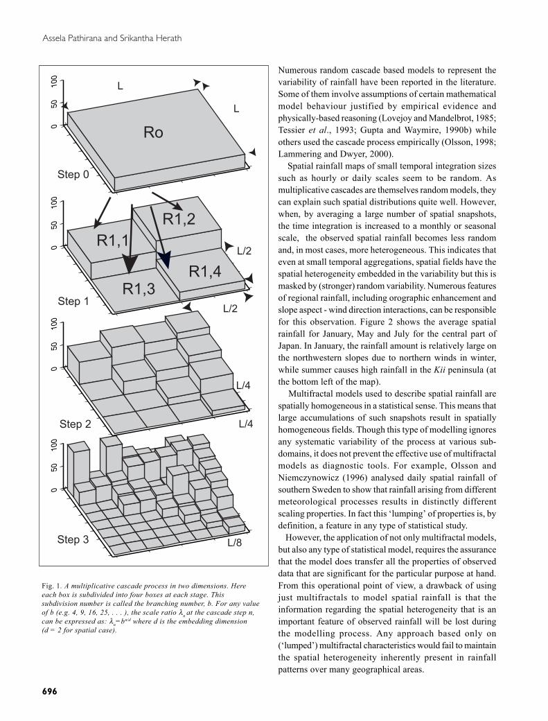
Numerous random cascade based models to represent thevariability of rainfall have been reported in the literature.Some of them involve assumptions of certain mathematicalmodel behaviour justified by empirical evidence andphysically-based reasoning (Lovejoy and Mandelbrot, 1985;Tessier et al., 1993; Gupta and Waymire, 1990b) whileothers used the cascade process empirically (Olsson, 1998;Lammering and Dwyer, 2000). Spatial rainfall maps of small temporal integration sizessuch as hourly or daily scales seem to be random. Asmultiplicative cascades are themselves random models, theycan explain such spatial distributions quite well. However,when, by averaging a large number of spatial snapshots,the time integration is increased to a monthly or seasonalscale, the observed spatial rainfall becomes less randomand, in most cases, more heterogeneous. This indicates thateven at small temporal aggregations, spatial fields have thespatial heterogeneity embedded in the variability but this ismasked by (stronger) random variability. Numerous featuresof regional rainfall, including orographic enhancement andslope aspect - wind direction interactions, can be responsiblefor this observation. Figure 2 shows the average spatialrainfall for January, May and July for the central part ofJapan. In January, the rainfall amount is relatively large onthe northwestern slopes due to northern winds in winter,while summer causes high rainfall in the Kii peninsula (atthe bottom left of the map). Multifractal models used to describe spatial rainfall arespatially homogeneous in a statistical sense. This means thatlarge accumulations of such snapshots result in spatiallyhomogeneous fields. Though this type of modelling ignoresany systematic variability of the process at various sub-domains, it does not prevent the effective use of multifractalmodels as diagnostic tools. For example, Olsson andNiemczynowicz (1996) analysed daily spatial rainfall ofsouthern Sweden to show that rainfall arising from differentmeteorological processes results in distinctly differentscaling properties. In fact this ‘lumping’ of properties is, bydefinition, a feature in any type of statistical study. However, the application of not only multifractal models,but also any type of statistical model, requires the assurancethat the model does transfer all the properties of observeddata that are significant for the particular purpose at hand.From this operational point of view, a drawback of usingjust multifractals to model spatial rainfall is that theinformation regarding the spatial heterogeneity that is animportant feature of observed rainfall will be lost duringthe modelling process. Any approach based only on(‘lumped’) multifractal characteristics would fail to maintainthe spatial heterogeneity inherently present in rainfallpatterns over many geographical areas.

050

100

050

100

050

100

050

100

Step 0

Step 3

Step 2

Step 1

Ro

R1,1R1,2

R1,3R1,4

L

L

L/2

L/2

L/4

L/4

L/8

Fig. 1. A multiplicative cascade process in two dimensions. Hereeach box is subdivided into four boxes at each stage. Thissubdivision number is called the branching number, b. For any valueof b (e.g. 4, 9, 16, 25, . . . ), the scale ratio λn

at the cascade step n,can be expressed as: λn=bn/d where d is the embedding dimension(d = 2 for spatial case).


697

In operational problems like flood risk analysis, theaccurate representation of spatial heterogeneity is asimportant as the precise modelling of spatial variability. Forexample, if an upstream mountainous area in a catchmentreceives significantly more rainfall than a low-lying areadownstream, flood magnitude and duration estimates forsuch a catchment can be substantially distorted by treatingspatial variability without considering spatial heterogeneityexplicitly. Jothityangkoon et al. (2000) incorporated spatialheterogeneity in multifractal simulation and evaluated theperformance of the model using spatial rainfall data fromAustralia. The explicit random cascade process used todistribute rainfall at sub-grid level, incorporated the spatialheterogeneity. In the present paper, a simpler method is usedto incorporate spatial heterogeneity in downscaled spatialrainfall and the outcome is compared with that of theJothityangkoon et al. (2000) method. The proposed modification can be used irrespective ofthe specific multifractal theory used to model the randomvariability of spatial rainfall. While numerous suitablemodels are available (Tessier et al., 1993; Meneveau andSreenivasan, 1987; Gupta and Waymire, 1990b; Deidda etal., 1999; Menabde et al. 1999; Lammering and Dwyer,2000), one with minimum complexity and wide applicationwas selected to demonstrate the proposed modification.

PROPOSED MODEL

Rainfall is considered a combined effect of two processes,(1) a multifractal process which is highly variable in spacebut, at least at regional and smaller scales, statisticallyuniform over the area concerned, and (2) a process thatrepresents the heterogeneity of rainfall in space that is usedto ‘modify’ the above multifractal process. The most general

case is that both these components should be stochastic(random). However, for simplicity, it is assumed that therandomness of the rainfall is provided solely by themultifractal component and the heterogeneity isdeterministic. At this stage, a rigorous physical interpretationof this separation is not attempted, though it is possible tovisualize it in the following way: The cloud positioning in aflat area small enough to ignore global circulation patterns,can be assumed to be random. However, when clouds moveover a land area with significant topographical features, thegeneration of rainfall is affected both by the position of thecloud and the topographical features such as mountains.This can be considered as a ‘modification’ of (random) cloudpositioning by a deterministic process that represents thelocal topography. (However, this localised effect may notbe caused only by the orography.) Hence, the rainfall over asmall period of time seems to be random because it is amixture of random and deterministic components. Whenthe rainfall is accumulated over a long time period, therandomness reduces to a uniform field due to the averagingeffect, and hence, the deterministic effect predominates. Thiscan explain the marked heterogeneity observed in largeaccumulations. As the accumulation length is increased, therandom effect becomes dormant and the heterogeneitybecomes more obvious. However, in practice, this is trueonly if similar rainfalls (e.g. same season) are accumulated.For example, if the rainfall of Japan is accumulated over allthe seasons, the winter and summer rainfalls maycompensate each other to a large degree, and produce a moreuniform field than the winter or summer rainfall takenseparately.

136º 138º 140º 142º

34º

36º

38º

0 100 200

km

136º 138º 140º 142º

34º

36º

38º

136º 138º 140º 142º

34º

36º

38º

0 100 200

km

136º 138º 140º 142º

34º

36º

38º

136º 138º 140º 142º

34º

36º

38º

0 100 200

km

136º 138º 140º 142º

34º

36º

38º

0

5

10

15

20

25

Fig. 2. Spatial heterogeneity shown by the daily average rainfall intensities for the months of January (left) May (middle) and July (right),based on radar-AMeDAS data from 1995 to 1999. Units: mm day-1


698

Mathematical developmentThe following equation expresses the proposed model inmathematical notation:

jijiji GMR ,,, = , =

=otherwiseGRGfor

Mjiji

jiji

,,

,, /

00 (1)

where Ri,j is the rainfall on the pixel (i,j) and Gi,j is thecomponent of that rainfall that is invariant over a longaccumulation. It is assumed that it can be representedadequately by the long-term seasonal average. Then, bydefinition, Mi,j is a component that is randomly distributedin the space so that M yields a uniform field at largeaccumulations. Hence M is a candidate for multifractalmodelling. To keep the model simple, the temporal progression ofthe rainfall is neglected. Thus, a key assumption of thepresent model is that the rainfall of a given snapshot isindependent of the other snapshots. For small time stepslike hourly rainfall, this may not be true, for the movementof rainfall over an area cannot be neglected at such a smalltemporal scale.

Rainfall dataThe operational radar rainfall composites (referred to asRadar-AMeDAS hereafter) published by the JapanMeteorological Agency (JMA), generally cover the wholeJapanese archipelago. JMA uses 19 conventional weatherradars with 400 km radial coverage (except for the Mt. Fujiradar which covers 800km) to provide hourly rainfallestimates at an average of 8 scans per hour. These data,with a resolution of 2.5 km are converted to 5 km resolutionand then calibrated with the extensive hourly rain gaugenetwork, popularly known as AMeDAS, to correct for errorsarising from the instability of the sensitivity of the radarhardware and due to the vertical variation of rainfall(Makihara, 1996). The final product is hourly-calibratedspatial rainfall data of land and surrounding sea with a gridsize of approximately 5km (0.06250 in longitude and 0.050

in latitude). An area of 128x128 pixels bounded by 39.65N134.5W, 33.3S and 142.4375E was selected for the study.The rainfall precision is 1mm (with an additional value at0.4mm). As the model takes no account of the temporal correlationof rainfall events that occurs at small accumulation sizes, itwas tested at a daily scale. Daily rainfall snapshots werecreated by summing the 24 hourly snapshots of the day. The spatial heterogeneity of rainfall varies with the season(Fig. 2). Hence, rainfall of different seasons must be

modelled separately, to capture the spatial heterogeneitycorrectly. In the present research, each month was modelledas a different season. Since the data for the period of 1995–1999 were available for analysis, the number of snapshotsavailable for model fitting for a given month was about 150.

Multifractal modelA multifractal model is needed to represent M (Eqn. 1). Theβ-lognormal model proposed by Over and Gupta (1996)was used because of its simplicity, wide application and theability to treat zero rainfall areas explicitly. Figure 1 shows an example of a multiplicative cascadeprocess. The branching number b is given by Ni+1/Ni

= bwhere Ni

is the total number of segments at cascade step i.At each cascade step, each segment is divided into b equalparts and each part is multiplied by a value (cascade weight)drawn from a specified distribution, which is known as thegenerator of the cascade. One of the simplest cascademodels is the β-model, whose generator is specified by:

β−−== bWP 1)0( , ββ −== bbWP )( (2)

where W is the cascade weight and b is a model parameter.This model can represent the presence and absence of valuesin a distribution. When a lognormal distribution is used asgenerator the resulting cascade is known as a lognormalcascade. Over and Gupta (1996) combined the above twocascade models to propose a b-lognormal model given by:

βσσβ −+−== bbWP

Xb

)( 2]log[2

β−−== bWP 1)0( (3)

where β and σ2 are model parameters. X is a standard normalvariable. This is a conserved cascade scheme, for theformulation maintains the expected value of W,

1)( =wE

PARAMETER EVALUATION FOR LOGNORMALMODEL

A multiplicative cascade shows the following scalingbehaviour:

∑ ==i

qqiRqM )(, ][),( τλ λλ (4)

where Ri,λ is the value of the field at the ith box at the scale

)1][0)1( 2/)log([ 2

==− +−− XbbEb σσβ

[()( 2/)log(2

+= +−−− XbbbEWE σσββ


699

λ (λ=L/l where l is scale and L is the largest scale of interest.)The order of statistical moment is q. Over and Gupta (1994, 1996) proposed the concept of aMandelbrot-Kahane-Peyriere (MKP) function to estimatemodel parameters for the β-lognormal model. MKPfunction, χ(q), of a multiplicative cascade process, is definedas the slope of the statistical moment M(λ,q) (Eqn. 4) to thecascade step n (Fig. 1). Given that the cascade follows the scaling lawM(λ,q)=λτ(q), the MKP function for the cascade is (bydefinition of the MKP function) τ(q)/d. Over and Gupta(1996) derived the following expression for the MKPfunction for the β-lognormal model:

)/()2/)ln(()1)(1()( 22 qqbqq −+−−= σβχ (5)

By considering the first and second derivatives of qχ withrespect to q, σ2 and β can be derived as follows:

)ln()()2(

2

bdqτσ = ;

2)12)(ln()(1

2)1( −++= qbd

q στβ (6)

where b is the branching number (Fig. 1), and d is theembedding dimension ( d=2, for spatial rainfall). The valuesof σ2 and β can be evaluated numerically by computing thevalue of derivatives of τ(q) at some value of q. It is customaryto use q=1 .

One of the main advantages of using the β-lognormalmodel to represent rainfall is its ability to incorporate non-rainy pixels explicitly. This avoids the problems related toapplying arbitrary cut-off intensities to introduce zero valuesto model generated fields. The use of the lognormalgenerator which has an analytical expression and thetransparent cascade scheme makes this an easy model toimplement. The use of lognormal cascades (which,mathematically is a special case of a broad class known asLévy-stable distributions.) to model rain fields, has beenquestioned in the literature (e.g. Tessier et al., 1993).However, this issue is still undecided and is outside the scopeof the present research.

Methodology for model constructionAs expressed in Eqn.1, the most important step in modelconstruction is to ‘filter’ the observed rain fields to obtainM fields, which are spatially homogeneous in a statisticalsense. To compute the field G for a given month, all thesnapshots for that month were averaged at pixel level as:

∑=

='

1,,, '

1 N

kkjiji R

NA (7)

∑=ji jijiji AATG

, ,,, / (8)

where N’ is the number of snapshots with the value (i, j)present and T is the total number of pixels in a snapshot. Inother words, Gi,j

is the field of normalized long-term averagesused to represent the spatial heterogeneity. For each snapshot, R, a field of M is obtained by applyingthe relationship in Eqn.1. After obtaining the M fields, thenext step was to test whether it is possible to model M as amultifractal model. Although rainfall distributions in two-dimensions have been verified as multifractal on numerousoccasions in the past, this is essential since M is only a fieldderived from observed rainfall, newly introduced in thepresent work.

SCALING OF M

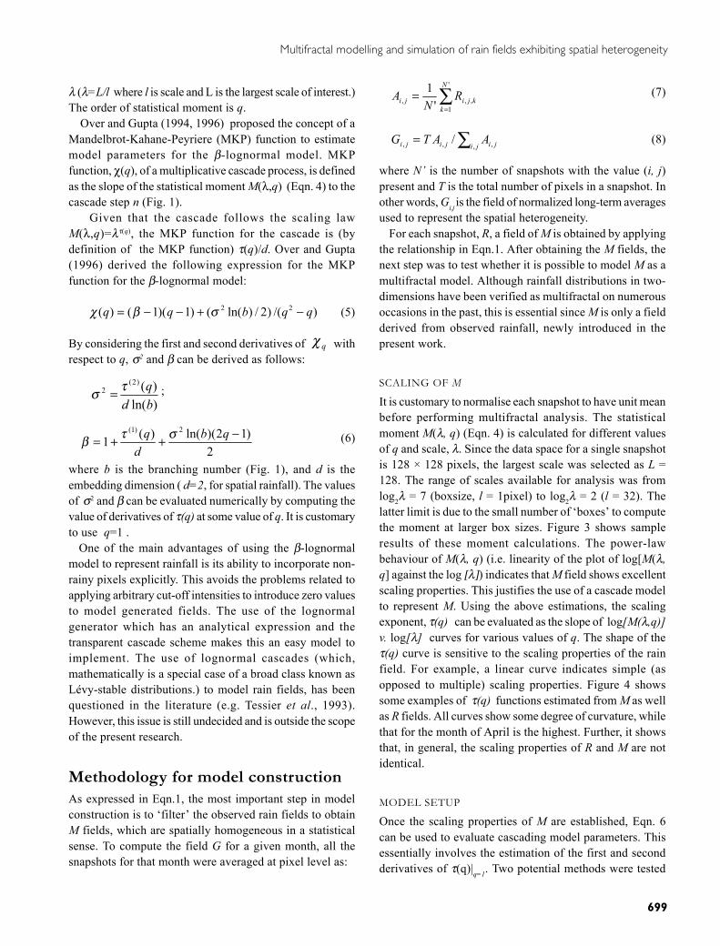
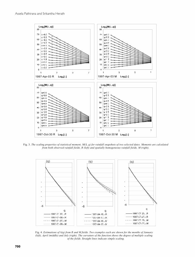
It is customary to normalise each snapshot to have unit meanbefore performing multifractal analysis. The statisticalmoment M(λ, q) (Eqn. 4) is calculated for different valuesof q and scale, λ. Since the data space for a single snapshotis 128 × 128 pixels, the largest scale was selected as L =128. The range of scales available for analysis was fromlog2λ = 7 (boxsize, l = 1pixel) to log2λ = 2 (l = 32). Thelatter limit is due to the small number of ‘boxes’ to computethe moment at larger box sizes. Figure 3 shows sampleresults of these moment calculations. The power-lawbehaviour of M(λ, q) (i.e. linearity of the plot of log[M(λ,q] against the log [λ]) indicates that M field shows excellentscaling properties. This justifies the use of a cascade modelto represent M. Using the above estimations, the scalingexponent, τ(q) can be evaluated as the slope of log[M(λ,q)]v. log[λ] curves for various values of q. The shape of theτ(q) curve is sensitive to the scaling properties of the rainfield. For example, a linear curve indicates simple (asopposed to multiple) scaling properties. Figure 4 showssome examples of τ(q) functions estimated from M as wellas R fields. All curves show some degree of curvature, whilethat for the month of April is the highest. Further, it showsthat, in general, the scaling properties of R and M are notidentical.

MODEL SETUP

Once the scaling properties of M are established, Eqn. 6can be used to evaluate cascading model parameters. Thisessentially involves the estimation of the first and secondderivatives of τ(q)|q=1. Two potential methods were tested


700

0

10

20

30

40

50

60

70

80

1 3 5 7

Log2[M(λ ,q)]

Log2[λ ]

q=6.0

q=2.0

q=2.5

q=3.0

q=3.5

q=4.0

q=4.5

q=5.0

q=5.5

q=1.0

q=1.5

q=0.5

q=0.0

1997-Apr-03 M

0

10

20

30

40

50

60

70

80

1 3 5 7

Log2[M(λ ,q)]

Log2[λ ]

q=6.0

q=2.0

q=2.5

q=3.0

q=3.5

q=4.0

q=4.5

q=5.0

q=5.5

q=1.0

q=1.5

q=0.5

q=0.0

1997-Apr-03 R

0

10

20

30

40

50

60

70

80

1 3 5 7

Log2[M(λ ,q)]

Log2[λ ]

q=6.0

q=2.0

q=2.5

q=3.0

q=3.5

q=4.0

q=4.5

q=5.0

q=5.5

q=1.0

q=1.5

q=0.5

q=0.0

1997-Oct-30 R

0

10

20

30

40

50

60

70

80

1 3 5 7

Log2[M(λ ,q)]

Log2[λ ]

q=6.0

q=2.0

q=2.5

q=3.0

q=3.5

q=4.0

q=4.5

q=5.0

q=5.5

q=1.0

q=1.5

q=0.5

q=0.0

1997-Oct-30 M

Fig. 3. The scaling properties of statistical moment, M(λ, q) for rainfall snapshots of two selected dates. Moments are calculatedfrom both observed rainfall fields, R (left) and spatially homogeneous rainfall fields, M (right).

-6

-

-

-

-

-

q

(q)

-6

-

-

-

-

-

q

(q)

-6

-

-

-

-

-

q

(q)

Fig. 4. Estimations of τ(q) from R and M fields. Two examples each are shown for the months of January(left), April (middle) and July (right). The curvature of the function shows the degree of multiple scaling

of the fields. Straight lines indicate simple scaling.


701

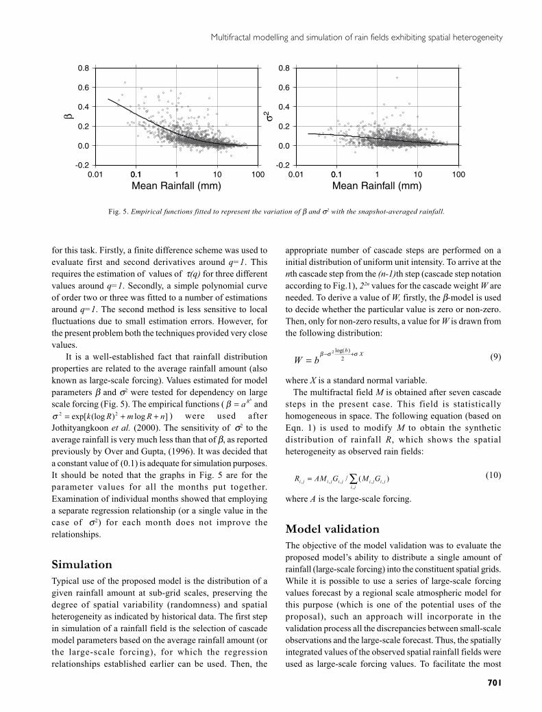
for this task. Firstly, a finite difference scheme was used toevaluate first and second derivatives around q=1. Thisrequires the estimation of values of τ(q) for three differentvalues around q=1. Secondly, a simple polynomial curveof order two or three was fitted to a number of estimationsaround q=1. The second method is less sensitive to localfluctuations due to small estimation errors. However, forthe present problem both the techniques provided very closevalues. It is a well-established fact that rainfall distributionproperties are related to the average rainfall amount (alsoknown as large-scale forcing). Values estimated for modelparameters β and σ2 were tested for dependency on largescale forcing (Fig. 5). The empirical functions (

bRa=β and]log)(logexp[ 22 nRmRk ++=σ ) were used after

Jothityangkoon et al. (2000). The sensitivity of σ2 to theaverage rainfall is very much less than that of β, as reportedpreviously by Over and Gupta, (1996). It was decided thata constant value of (0.1) is adequate for simulation purposes.It should be noted that the graphs in Fig. 5 are for theparameter values for all the months put together.Examination of individual months showed that employinga separate regression relationship (or a single value in thecase of σ2) for each month does not improve therelationships.

SimulationTypical use of the proposed model is the distribution of agiven rainfall amount at sub-grid scales, preserving thedegree of spatial variability (randomness) and spatialheterogeneity as indicated by historical data. The first stepin simulation of a rainfall field is the selection of cascademodel parameters based on the average rainfall amount (orthe large-scale forcing), for which the regressionrelationships established earlier can be used. Then, the

appropriate number of cascade steps are performed on ainitial distribution of uniform unit intensity. To arrive at thenth cascade step from the (n-1)th step (cascade step notationaccording to Fig.1), 22n values for the cascade weight W areneeded. To derive a value of W, firstly, the β-model is usedto decide whether the particular value is zero or non-zero.Then, only for non-zero results, a value for W is drawn fromthe following distribution:

Xb

bWσσβ +−

= 2)log(2

(9)

where X is a standard normal variable.The multifractal field M is obtained after seven cascade

steps in the present case. This field is statisticallyhomogeneous in space. The following equation (based onEqn. 1) is used to modify M to obtain the syntheticdistribution of rainfall R, which shows the spatialheterogeneity as observed rain fields:

∑=ji

jijijijiji GMGMAR,

,,,,, )(/ (10)

where A is the large-scale forcing.

Model validationThe objective of the model validation was to evaluate theproposed model’s ability to distribute a single amount ofrainfall (large-scale forcing) into the constituent spatial grids.While it is possible to use a series of large-scale forcingvalues forecast by a regional scale atmospheric model forthis purpose (which is one of the potential uses of theproposal), such an approach will incorporate in thevalidation process all the discrepancies between small-scaleobservations and the large-scale forecast. Thus, the spatiallyintegrated values of the observed spatial rainfall fields wereused as large-scale forcing values. To facilitate the most

-0.2

0.0

0.2

0.4

0.6

0.8β

0.01 0.10.1 1 10 100

Mean Rainfall (mm)

-0.2

0.0

0.2

0.4

0.6

0.8

σ2

0.01 0.10.1 1 10 100

Mean Rainfall (mm)

Fig. 5. Empirical functions fitted to represent the variation of β and σ2 with the snapshot-averaged rainfall.


702

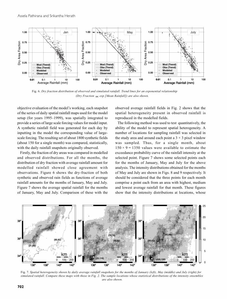
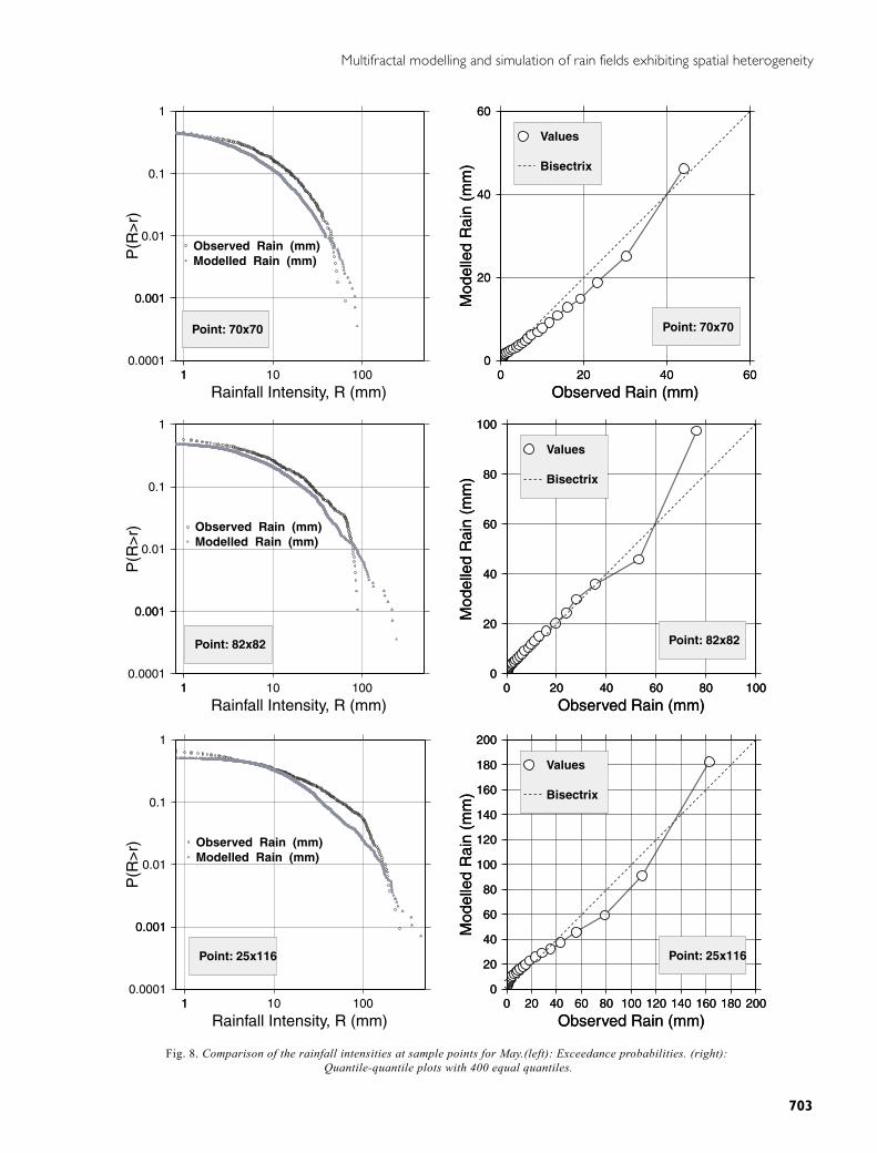
objective evaluation of the model’s working, each snapshotof the series of daily spatial rainfall maps used for the modelsetup (for years 1995–1999), was spatially integrated toprovide a series of large scale forcing values for model input.A synthetic rainfall field was generated for each day byinputting in the model the corresponding value of large-scale forcing. The resulting set of about 1800 synthetic fields(about 150 for a single month) was compared, statistically,with the daily rainfall snapshots originally observed. Firstly, the fraction of dry areas was compared in modelledand observed distributions. For all the months, thedistribution of dry fraction with average rainfall amount formodelled rainfall showed close agreement withobservations. Figure 6 shows the dry-fraction of bothsynthetic and observed rain fields as functions of averagerainfall amounts for the months of January, May and July.Figure 7 shows the average spatial rainfall for the monthsof January, May and July. Comparison of these with the

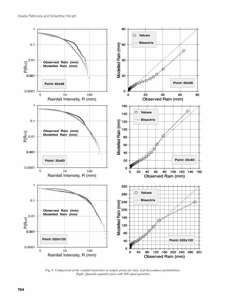
observed average rainfall fields in Fig. 2 shows that thespatial heterogeneity present in observed rainfall isreproduced in the modelled fields. The following method was used to test quantitatively, theability of the model to represent spatial heterogeneity. Anumber of locations for sampling rainfall was selected inthe study area and around each point a 3 × 3 pixel windowwas sampled. Thus, for a single month, about150 × 9 = 1350 values were available to estimate theexceedance probability curve of the rainfall intensity at theselected point. Figure 7 shows some selected points eachfor the months of January, May and July for the aboveanalysis. The intensity distributions obtained for the monthsof May and July are shown in Figs. 8 and 9 respectively. Itshould be considered that the three points for each monthcomprise a point each from an area with highest, mediumand lowest average rainfall for that month. These figuresshow that the intensity distributions at locations, whose

0.00

0.25

0.50

0.75

1.00

Dry

Are

a Fr

actio

n0.010.01 0.1 1 10 100

Average Rainfall (mm)

0.00

0.25

0.50

0.75

1.00

0.010.01 0.1 1 10 100


ObservedModeledObs (Trend)Mod (Trend)

0.00

0.25

0.50

0.75

1.00

Dry

Are

a Fr

actio

n

0.010.01 0.1 1 10 100


0.00

0.25

0.50

0.75

1.00

0.010.01 0.1 1 10 100


ObservedModeledObs (Trend)Mod (Trend)

May July

0.00

0.25

0.50

0.75

1.00

0.010.01 0.1 1 10 100

0.00

0.25

0.50

0.75

1.00

0.010.01 0.1 1 10 100

ObservedModeledObs (Trend)Mod (Trend)D

ry A

rea

Frac

tion


Jan

Fig. 6. Dry fraction distribution of observed and simulated rainfall. Trend lines for an exponential relationship(Dry Fraction ∝ exp [Mean Rainfall]) are also shown.

136º 138º 140º 142º

34º

36º

38º

0 100 200

km

(60,68)

(35,83)

(020,120)

136º 138º 140º 142º

34º

36º

38º

136º 138º 140º 142º

34º

36º

38º

0 100 200

km

(70,70)

(82,82)

(25,116)

136º 138º 140º 142º

34º

36º

38º

136º 138º 140º 142º

34º

36º

38º

0 100 200

km

(85,82)

(21,83)

136º 138º 140º 142º

34º

36º

38º

0

5

10

15

20

25

Fig. 7. Spatial heterogeneity shown by daily average rainfall snapshots for the months of January (left), May (middle) and July (right) forsimulated rainfall. Compare these maps with those in Fig. 2. The sample locations whose statistical distributions of the intensity ensembles

are also shown.


703

0.0001

0.0010.001

0.01

0.1

1

P(R

>r)

11 10 100

Rainfall Intensity, R (mm)

Observed Rain (mm)Modelled Rain (mm)

Point: 82x82

0

20

40

60

80

100

Mod

elle

d R

ain

(mm

)

0 20 40 60 80 100

Observed Rain (mm)

0

20

40

60

80

100

Mod

elle

d R

ain

(mm

)

0 20 40 60 80 100

Observed Rain (mm)

Values

Point: 82x82

Bisectrix

0.0001

0.0010.001

0.01

0.1

1

P(R

>r)

11 10 100



0

20

40

60

Mod

elle

d R

ain

(mm

)

0 20 40 60

Observed Rain (mm)

0

20

40

60

Mod

elle

d R

ain

(mm

)

0 20 40 60

Observed Rain (mm)

Values

Point: 70x70

Bisectrix

0.0001

0.0010.001

0.01

0.1

1

P(R

>r)

11 10 100



0

20

40

60

80

100

120

140

160

180

200

Mod

elle

d R

ain

(mm

)

0 20 40 60 80 100 120 140 160 180 200

Observed Rain (mm)

0

20

40

60

80

100

120

140

160

180

200

Mod

elle

d R

ain

(mm

)

0 20 40 60 80 100 120 140 160 180 200

Observed Rain (mm)

Values

Point: 25x116

Bisectrix

Point: 70x70

Point: 25x116

Fig. 8. Comparison of the rainfall intensities at sample points for May.(left): Exceedance probabilities. (right):Quantile-quantile plots with 400 equal quantiles.


704

0

20

40

60

80

Mod

elle

d R

ain

(mm

)

0 20 40 60 80

Observed Rain (mm)

0

20

40

60

80

Mod

elle

d R

ain

(mm

)

0 20 40 60 80

Observed Rain (mm)

Values

Point: 60x68

Bisectrix

0

20

40

60

80

100

120

140

160

Mod

elle

d R

ain

(mm

)

0 20 40 60 80 100 120 140 160

Observed Rain (mm)

0

20

40

60

80

100

120

140

160

Mod

elle

d R

ain

(mm

)

0 20 40 60 80 100 120 140 160

Observed Rain (mm)

Values

Point: 35x83

Bisectrix

0

40

80

120

160

200

240

280

320

Mod

elle

d R

ain

(mm

)

0 40 80 120 160 200 240 280 320

Observed Rain (mm)

0

40

80

120

160

200

240

280

320

Mod

elle

d R

ain

(mm

)

0 40 80 120 160 200 240 280 32

Observed Rain (mm)

Values

Point: 020x120

Bisectrix

0.0001

0.0010.001

0.01

0.1

1P

(R>r

)

11 10 100



0.0001

0.0010.001

0.01

0.1

1

P(R

>r)

11 10 100



0.0001

0.0010.001

0.01

0.1

1

P(R

>r)

11 10 100



Point: 60x68

Point: 35x83

Point: 020x120

Fig. 9. Comparison of the rainfall intensities at sample points for July. Left:Exceedance probabilities.Right: Quantile-quantile plots with 400 equal quantiles.


705

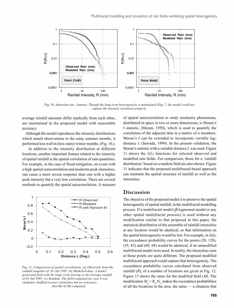
average rainfall amounts differ markedly from each other,are maintained in the proposed model with reasonableaccuracy. Although the model reproduces the intensity distributionswhich match observations in the rainy summer months, itperformed less well in (less-rainy) winter months. (Fig. 10.). In addition to the intensity distribution at differentlocations, another important feature related to the intensityof spatial rainfall is the spatial correlation of rain quantities.For example, in the case of flood mitigation, an event witha high spatial autocorrelation and moderate peak intensities,can cause a more severe response than one with a higherpeak intensity but a very low correlation. There are severalmethods to quantify the spatial autocorrelation. A measure

of spatial autocorrelation to study stochastic phenomena,distributed in space in two or more dimensions, is Moran’sI statistic, (Moran, 1950), which is used to quantify thecorrelation of the adjacent data in a matrix of n members.Moran’s I can be extended to incorporate variable lag-distance L (Sawada, 1999). In the present validation, theMoran’s statistic with a variable distance L was used. Figure11 shows the I(L) functions for selected observed andmodelled rain fields. For comparison, those for a ‘rainfalldistribution’ based on a random field are also shown. Figure11 indicates that the proposed multifractal-based approachcan maintain the spatial structure of rainfall as well as theintensities.

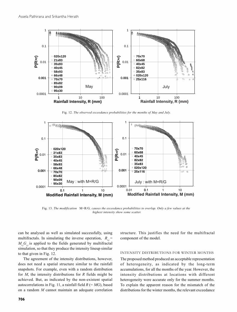
DiscussionThe objective of the proposed model is to preserve the spatialheterogeneity of spatial rainfall, in the multifractal modellingprocess. If a multifractal model (β-lognormal model or anyother spatial multifractal process) is used without anymodification similar to that proposed in this paper, thestatistical distribution of the ensemble of rainfall intensitiesat any location would be identical, so that information onthe spatial heterogeneity would be lost. For example, in July,the exceedance probability curves for the points (20, 120),(35, 83) and (60, 68) would be identical, if an unmodifiedmultifractal model were used. In reality, the intensities seenat those points are quite different. The proposed modifiedmultifractal approach could capture that heterogeneity. Theexceedance probability curves calculated from observedrainfall (R), of a number of locations are given in Fig. 12.Figure 13 shows the same for the modified field (M). Themodification Mi,j

= Ri,j/Gi,j makes the exceedance probabilities

of all the locations in the area, the same — a situation that

0.0001

0.0010.001

0.01

0.1

1

P(R

>r)

11 10 100



Point: 21x83

0.0001

0.0010.001

0.01

0.1

1

P(R

>r)

11 10 100



Point: 85x82

Fig. 10. Intensities for January. Though the long-term heterogeneity is maintained (Fig. 7, the model could notcapture the intensity variations properly.

-0.2

0

0.2

0.4

0.6

0.8

1

0 0.1 0.2 0.3 0.4 0.5 0.6Distance L (Deg.)

Mor

an's

I

R ObservedR ModeledR with Random M

Fig. 11. Comparison of spatial correlations. (a) Observed: from therainfall snapshot of 01-Jul-1995. (b) Modelled data: A model-generated field with the large scale forcing as the average rainfallof 01-Jul-1995. (c) Random: The field computed for case b wasrandomly shuffled (correct intensities but no structure),

then R(=G M) computed.


706

can be analysed as well as simulated successfully, usingmultifractals. In simulating the inverse operation, Ri,j

=Mi,jGi,j

is applied to the fields generated by multifractalsimulation, so that they produce the intensity lineup similarto that given in Fig. 12. The agreement of the intensity distributions, however,does not need a spatial structure similar to the rainfallsnapshots. For example, even with a random distributionfor M, the intensity distributions for R fields might beachieved. But, as indicated by the non-existent spatialautocorrelations in Fig. 11, a rainfall field R (= MG), basedon a random M cannot maintain an adequate correlation

0.0001

0.0010.001

0.01

0.1

1

11 10 100

## ## ## ## ############################################################################################################################################################################################################################################################################################################################################################################################################################################################

#

xx xx xx xx xxxxxxxxxxxxxxxxxxxxxxxxxxxxxxxxxxxxxxxxxxxxxxxxxxxxxxxxxxxxxxxxxxxxxxxxxxxxxxxxxxxxxxxxxxxxxxxxxxxxxxxxxxxxxxxxxxxxxxxxxxxxxxxxxxxxxxxxxxxxxxxxxxxxxxxxxxxxxxxxxxxxxxxxxxxxxxxxxxxxxxxxxxxxxxxxxxxxxxxxxxxxxxxxxxxxxxxxxxxxxxxxxxxxxxxxxxxxxxxxxxxxxxxxxxxxxxxxxxxxxxxxxxxxxxxxxxxxxxxxxxxxxxxxxxxxxxxxxxxxxxxxxxxxxxxxxxxxxxxxxxxxxxxxxxxxxxxxxxxxxxxxxxxxxxxxxxxxxxxxxxxxxxxxxxxxxxxxxxxxxxxxxxxxxxxxxxxxxxxxxxxxxxxxxxxxxxxxxxxxxxxxxxxxxxxxxxxxxxxxxxxxxxxxxxxx

x

** ** ** ** ** ***************************************************************************************************************************************************************************************************************************************************************************************************************************************************************************************************************************************************************************************************************************************

*****

**

*

// // // // // // // // // // //////////////////////////////////////////////////////////////////////////////////////////////////////////////////////////////////////////////////////////////////////////////////////////////////////////////////////////////////////////////////////////////////////////////////////////////////////////////////////////////////////////////////////////////////////////////////////////////////////////////////////////////////////////// //////////////////// //////////////// //////////////////

/

020x12021x8335x8340x4558x9366x48#

70x7085x82x

90x09*

95x30/


July

P(R

>r)


May

P(R

>r)

0.0001

0.0010.001

0.01

0.1

1

11 10 100

## ## ## ############################################################################################################################################################################################################################################################################################################################################################################################################################################################################################################################################################################################################################################################################################################################################################################################################################################################################################################################ ################

#

70x7060x6840x4582x8235x83020x120#

25x116

Fig. 12. The observed exceedance probabilities for the months of May and July.

0.0001

0.0010.001

0.01

0.1

1

0.01 0.10.1 1 10

## ## ############################################################################################################################################################################################################################################################################################################################################################################################################################################################################################################################################################################################################################################################################################################################################################################################################################################################################################################################## ################

#

70x7060x6840x4582x8235x83020x120#

25x116

0.0001

0.0010.001

0.01

0.1

1

0.10.1 1 10

## ## ## ##############################################################################################################################################################################################################################################################################################################################################################################################################################################################

#

xx xx xx xx xxxxxxxxxxxxxxxxxxxxxxxxxxxxxxxxxxxxxxxxxxxxxxxxxxxxxxxxxxxxxxxxxxxxxxxxxxxxxxxxxxxxxxxxxxxxxxxxxxxxxxxxxxxxxxxxxxxxxxxxxxxxxxxxxxxxxxxxxxxxxxxxxxxxxxxxxxxxxxxxxxxxxxxxxxxxxxxxxxxxxxxxxxxxxxxxxxxxxxxxxxxxxxxxxxxxxxxxxxxxxxxxxxxxxxxxxxxxxxxxxxxxxxxxxxxxxxxxxxxxxxxxxxxxxxxxxxxxxxxxxxxxxxxxxxxxxxxxxxxxxxxxxxxxxxxxxxxxxxxxxxxxxxxxxxxxxxxxxxxxxxxxxxxxxxxxxxxxxxxxxxxxxxxxxxxxxxxxxxxxxxxxxxxxxxxxxxxxxxxxxxxxxxxxxxxxxxxxxxxxxxxxxxxxxxxxxxxxxxxxxxxxxxxxxxxx

x

** ** ** ** *****************************************************************************************************************************************************************************************************************************************************************************************************************************************************************************************************************************************************************************************************************************************

*****

**

*

// // // // // // // // // ////////////////////////////////////////////////////////////////////////////////////////////////////////////////////////////////////////////////////////////////////////////////////////////////////////////////////////////////////////////////////////////////////////////////////////////////////////////////////////////////////////////////////////////////////////////////////////////////////////////////////////////////////////////// //////////////////////////////////// //////////////////

/

020x12021x8335x8340x4558x9366x48#

70x7085x82x

90x09*

95x30/

Modified Rainfall Intensity, M (mm)

July : with M=R/G

P(R

>r)


May : with M=R/G

P(R

>r)

Fig. 13. The modification M=R/G, causes the exceedance probabilities to overlap. Only a few values at thehighest intensity show some scatter.

structure. This justifies the need for the multifractalcomponent of the model.

INTENSITY DISTRIBUTIONS FOR WINTER MONTHS

The proposed method produced an acceptable representationof heterogeneity, as indicated by the long-termaccumulations, for all the months of the year. However, theintensity distributions at locations with differentheterogeneity were accurate only for the summer months.To explain the apparent reason for the mismatch of thedistributions for the winter months, the relevant exceedance


707

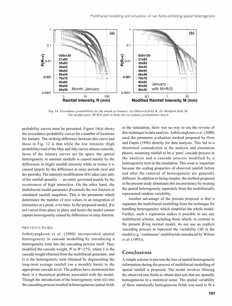
probability curves must be presented. Figure 14(a) showsthe exceedance probability curves for a number of locationsfor January. The striking difference between this curve andthose in Fig. 12 is that while the low intensity (highprobability) end of the May and July curves almost coincide,those of the January curves are far apart; the spatialheterogeneity in summer rainfalls is caused mainly by thedifferences in (high) rainfall intensity while in winter it iscaused largely by the difference in rainy periods (wet anddry periods). The intensity modification M/G takes care onlyof the rainfall quantity — an entity governed mainly by theoccurrences of high intensities. On the other hand, themultifractal model parameter β controls the wet fraction insimulated rainfall snapshots. This is the parameter whichdetermines the number of zero values in an integration ofintensities at a point, over time. In the proposed model, β isnot varied from place to place and hence the model cannotcapture heterogeneity caused by differences in rainy fraction.

PREVIOUS WORK

Jothityangkoon et al. (2000) incorporated spatialheterogeneity in cascade modelling by introducing aheterogeneity term into the cascading process itself. Theymodified the cascade weight, W as W=L*G, where L is thecascade weight obtained from the multifractal generator, andG is the heterogeneity term obtained by degenerating thelong-term average rainfall (on a monthly basis) to theappropriate cascade level. The authors have mentioned thatthere is a theoretical problem associated with the model.Though the introduction of the heterogeneity term (G) intothe cascading process resulted in heterogeneous spatial fields

in the simulation, there was no way to use the reverse ofthis technique in data analysis. Jothityangkoon et al. (2000)used the parameter evaluation method proposed by Overand Gupta (1996) directly for data analysis. This led to atheoretical contradiction in the analysis and simulationphases, assuming rainfall to be a ‘pure’ cascade process inthe analysis and a cascade process modified by aheterogeneity term in the simulation. This issue is importantbecause the scaling properties of observed rainfall beforeand after the removal of heterogeneity are generallydifferent. In addition to being simpler, the method proposedin the present study eliminates this inconsistency by treatingthe spatial heterogeneity separately from the multifractallyrepresented random variability. Another advantage of the present proposal is that itseparates the multifractal modelling from the technique forhandling heterogeneity, which simplifies the whole model.Further, such a separation makes it possible to use anymultifractal scheme, including those which, in contrast tothe present β-log normal model, do not use an explicitcascading process to represent the variability (M) in themodel (e.g. ‘continuous’ multifractals introduced by Wilsonet al. (1991)).

ConclusionsA simple scheme to prevent the loss of spatial heterogeneityinformation during the process of multifractal modelling ofspatial rainfall is proposed. The model involves filteringthe observed rain fields to obtain data sets that are spatiallyhomogeneous in a statistical sense. The spatial variabilityof these statistically homogeneous fields was used to fit a

0.0001

0.0010.001

0.01

0.1

1

11 10 100

### ## ## ## ################################################################################################################################################################################################################################################################################################################################################################################################################################################################################################################################################################################################################################################################################################################################################################################################################################################################################################################################################################################################################################################################################################################################################################################################################################

#

xx xx xx xx xxxxxxxxxxxxxxxxxxxxxxxxxxxxxxxxxxxxxxxxxxxxxxxxxxxxxxxxxxxxxxxxxxxxxxxxxxxxxxxxxxxxxxxxxxxxxxxxxxxxxxxxxxxxxxxxxxxxxxxxxxxxxxxxxxxxxxxxxxxxxxxxxxxxxxxxxxxxxxxxxxxxxxxxxxxxxxxxxxxxxxxxxxxxxxxxxxxxxxxxxx

xxxxxx

x

** ** ** ** ** ** ************************************************************************************************************************************************************************************************************************************************************************************************************************************************************************************************************************************************************************************************************************************************************************************************************************************************************************************************************************************************************************************************************************************************************************************************

*

// // // // // // // // // // //////////////////////////////////////////////////////////////////////////////////////////////////////////////////////////////////////////////////////////////////////////////////////////////////////////////////////////////////////////////////////////////////////////////////////////////////////////////////////////////////////////////////////////////////////////////////////////////////////////////////////////////

/

020x12021x8335x8340x4558x9366x48#

70x7085x82x

90x09*

95x30/

0.0001

0.0010.001

0.01

0.1

1

0.10.1 1 10

### ## ##################################################################################################################################################################################################################################################################################################################################################################################################################################################################################################################################################################################################################################################################################################################################################################################################################################################################################################################################################################################################################################################################################################################################################################################################################################

#

xx xx xx xx xxxxxxxxxxxxxxxxxxxxxxxxxxxxxxxxxxxxxxxxxxxxxxxxxxxxxxxxxxxxxxxxxxxxxxxxxxxxxxxxxxxxxxxxxxxxxxxxxxxxxxxxxxxxxxxxxxxxxxxxxxxxxxxxxxxxxxxxxxxxxxxxxxxxxxxxxxxxxxxxxxxxxxxxxxxxxxxxxxxxxxxxxxxxxxxxxxxxxxxxxx

xxxxxx

x

** ** ** ** ** **************************************************************************************************************************************************************************************************************************************************************************************************************************************************************************************************************************************************************************************************************************************************************************************************************************************************************************************************************************************************************************************************************************************************************************************************

*

// // // // // // // // // ////////////////////////////////////////////////////////////////////////////////////////////////////////////////////////////////////////////////////////////////////////////////////////////////////////////////////////////////////////////////////////////////////////////////////////////////////////////////////////////////////////////////////////////////////////////////////////////////////////////////////////////////

/

020x12021x8335x8340x4558x9366x48#

70x7085x82x

90x09*

95x30/

P(R

>r)


Month: January


January : with M=R/G

(a) (b)

P(R

>r)

Fig. 14. Exceedance probabilities for the month of January. (a) Observed field, R. (b) Modified field, MThe modification M=R/G fails to make the exceedance probabilities match.


708

multifractal model. The simulation process was the exactopposite of the above; using the multifractal model, spatiallyhomogeneous fields were simulated and later these were‘modified’ to add the spatial heterogeneity. It was assumedthat the spatial heterogeneity can be represented accuratelyby the normalised long-term average rainfall. The model disaggregated the rainfall of Japan accuratelyand maintained at the simulation stage the largeheterogeneity shown by the observations. However, themodel did not produce the intensity distributions at differentplaces accurately for the winter months because theheterogeneity of summer rainfall is caused mainly bydifferences in intensity while that of winter rainfall is dueto the differences in rainy periods at different spatiallocations. The present model can handle only theheterogeneity caused by the former situation.

ReferencesDeidda, R., Benzi, R. and Siccardi, F., 1999. Multifractal modeling

of anomalous scaling laws in rainfall. Water Resour. Res., 35,1853–1867.

Gupta, V.K. and Waymire, E., 1990b. Multiscaling properties ofspatial rainfall and river flow distributions. J. Geophys. Res.,95, 1999–2009.

Jothityangkoon, C., Sivapalan, M. and Viney, N.R., 2000. Testsof a space-time model of rainfall in southwestern Australia basedon nonhomogeneous random cascades. Water Resour. Res., 36,267–284.

Lammering, B. and Dwyer, I., 2000. Improvement of water balancein land surface schemes by random cascade disaggregation ofrainfall. Int. J. Climatol., 20, 681–695.

Lovejoy, S. and Mandelbrot, B.B., 1985. Fractal properties of rain,and a fractal model. Tellus, 37A, 209–232.

Makihara, Y., 1996. A method for improving radar estimates ofprecipitation by comparing data from radars and raingauges. J.Meteorol. Soc. Japan, 74, 459–480.

Menabde, M., Seed, A., Harris, D. and Pegram, G., 1999.Multiaffine random field model for rainfall. Water Resour. Res.,35, 509–514.

Meneveau, C. and Sreenivasan, K. R., 1987. Simple multifractalcascade model for fully developed turbulence. Phys. Rev. Lett.,59, 1424–1427.

Moran, P.A.P., 1950. Notes on continuous stochastic phenomena,Biometrika, 37.

Olsson, J., 1998. Evaluation of a scaling cascade model fortemporal rainfall-disaggregation. Hydrol. Earth Syst. Sci., 2,19–30.

Olsson, J. and Niemczynowicz, J., 1996. Multifractal analysis ofdaily spatial rainfall distributions. J. Hydrol., 187, 29–43.

Over, T.M. and Gupta, V.K., 1994. Statistical analysis of mesoscalerainfall: Dependence of a random cascade generator on large-scale forcing. J. Appl. Meteorol., 33, 1526–1542.

Over, T.M. and Gupta, V.K., 1996. A space-time theory ofmesoscale rainfall using random cascades. J. Geophys. Res.,101, 26,319–26,331.

Sawada, M., 1999. ROOKCASE: an excel 97/2000 visual basic(vb) add-in for exploring global and local spatial autocorrelation,Bull. Ecol. Soc. Amer., 80, 231–234. url: http://www.uottawa.ca/academic/arts/geographie /lpcweb /newlook/data_and_downloads/download/sawsoft/rooks.htm.

Shuttleworth, W.J., 1988. Evaporation from Amazonian rainforest.Proc. Roy. Soc. London Ser. B, 233, 321–346.

Tessier, Y., Lovejoy, S. and Schertzer, D., 1993. Universalmultifractals: theory and observations for rain and clouds. J.Appl. Meteorol., 2, 223–250.

Wilson, J., Schertzer, D. and Lovejoy, S., 1991. Continuousmultiplicative cascade model of rain and clouds. In: Non-linearvariability in geophysics: Scaling and Fractals, D. Schertzerand S. Lovejoy (Eds.). Kluwer, Dordrecht, The Netherlands.185–207.

Documents

Multifractal modelling and simulation of rain fields