Multiple Linear Regression & AIC

“I've come loaded with statistics, for I've noticed that a man can't prove anything without statistics. No man can.”

Mark Twain (Humorist & Writer)

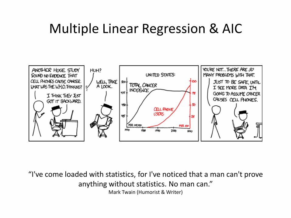
Linear Regression Linear relationships

Equation of a line: 𝑦 = 𝑚𝑥 + 𝑏

𝑚 = slope of the line 𝑅𝐼𝑆𝐸

𝑅𝑈𝑁

𝑏 = 𝑦-intercept

Regression Analysis PART 1: find a relationship between response variable (Y) and a predictor variable (X)

(e.g. Y~X)

PART 2: use relationship to predict Y from X

predictor (x)

resp

on

se (

y)

m

b Simple Linear Regression in R: lm(response~predictor)

summary(lm(response~predictor))

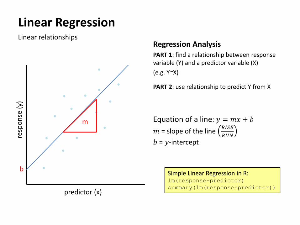
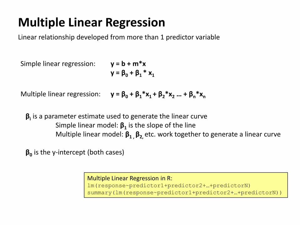
Multiple Linear Regression Linear relationship developed from more than 1 predictor variable

Simple linear regression: y = b + m*x y = β0 + β1 * x1

Multiple linear regression: y = β0 + β1*x1 + β2*x2 … + βn*xn

βi is a parameter estimate used to generate the linear curve Simple linear model: β1 is the slope of the line Multiple linear model: β1 , β2, etc. work together to generate a linear curve β0 is the y-intercept (both cases)

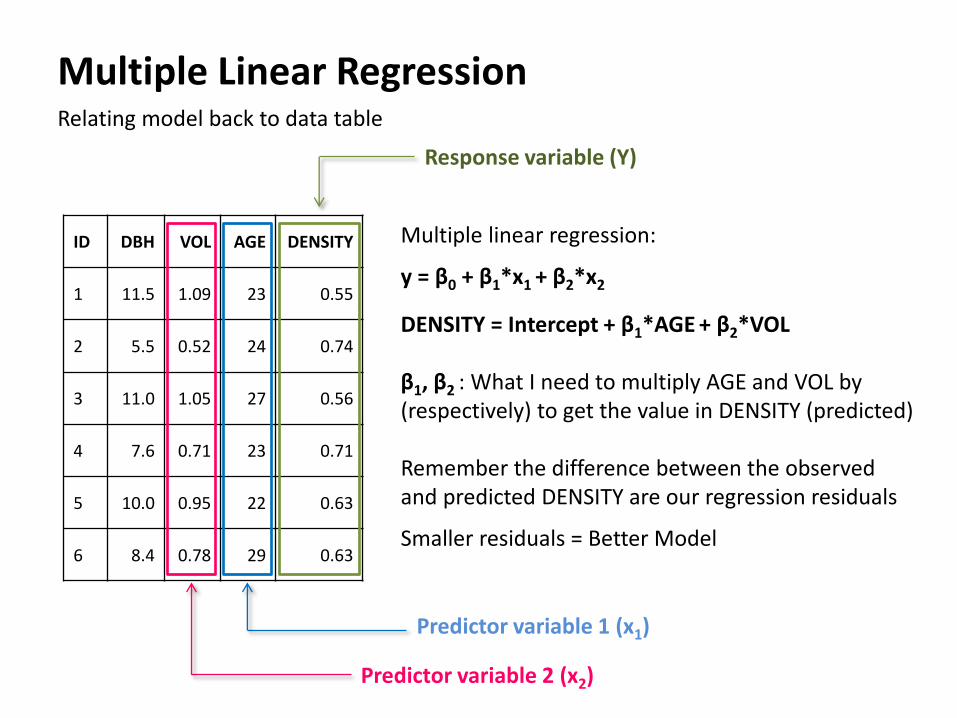
Multiple Linear Regression

ID DBH VOL AGE DENSITY

1 11.5 1.09 23 0.55

2 5.5 0.52 24 0.74

3 11.0 1.05 27 0.56

4 7.6 0.71 23 0.71

5 10.0 0.95 22 0.63

6 8.4 0.78 29 0.63

Relating model back to data table

Response variable (Y)

Predictor variable 2 (x2)

Predictor variable 1 (x1)

Multiple linear regression:

y = β0 + β1*x1 + β2*x2

DENSITY = Intercept + β1*AGE + β2*VOL β1, β2 : What I need to multiply AGE and VOL by (respectively) to get the value in DENSITY (predicted) Remember the difference between the observed and predicted DENSITY are our regression residuals

Smaller residuals = Better Model

Multiple Linear Regression Linear relationship developed from more than 1 predictor variable

Multiple Linear Regression in R: lm(response~predictor1+predictor2+…+predictorN)

summary(lm(response~predictor1+predictor2+…+predictorN))

Simple linear regression: y = b + m*x y = β0 + β1 * x1

Multiple linear regression: y = β0 + β1*x1 + β2*x2 … + βn*xn

βi is a parameter estimate used to generate the linear curve Simple linear model: β1 is the slope of the line Multiple linear model: β1 , β2, etc. work together to generate a linear curve β0 is the y-intercept (both cases)

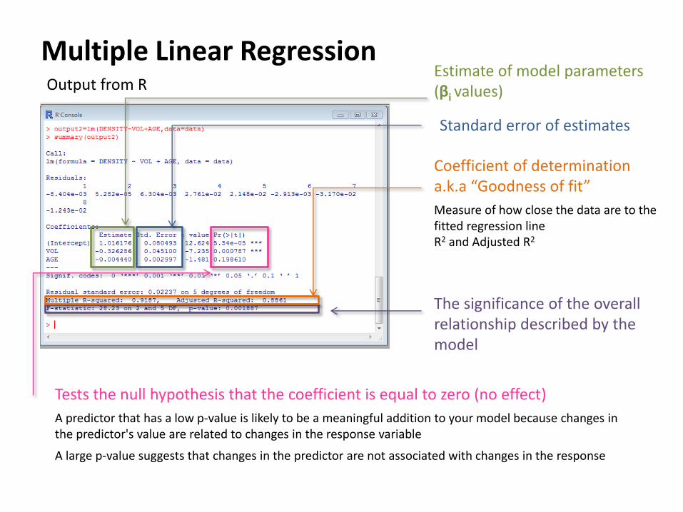
Multiple Linear Regression Output from R

Estimate of model parameters (βi values)

Standard error of estimates

Tests the null hypothesis that the coefficient is equal to zero (no effect)

A predictor that has a low p-value is likely to be a meaningful addition to your model because changes in the predictor's value are related to changes in the response variable

A large p-value suggests that changes in the predictor are not associated with changes in the response

Coefficient of determination a.k.a “Goodness of fit”

Measure of how close the data are to the fitted regression line R2 and Adjusted R2

The significance of the overall relationship described by the model

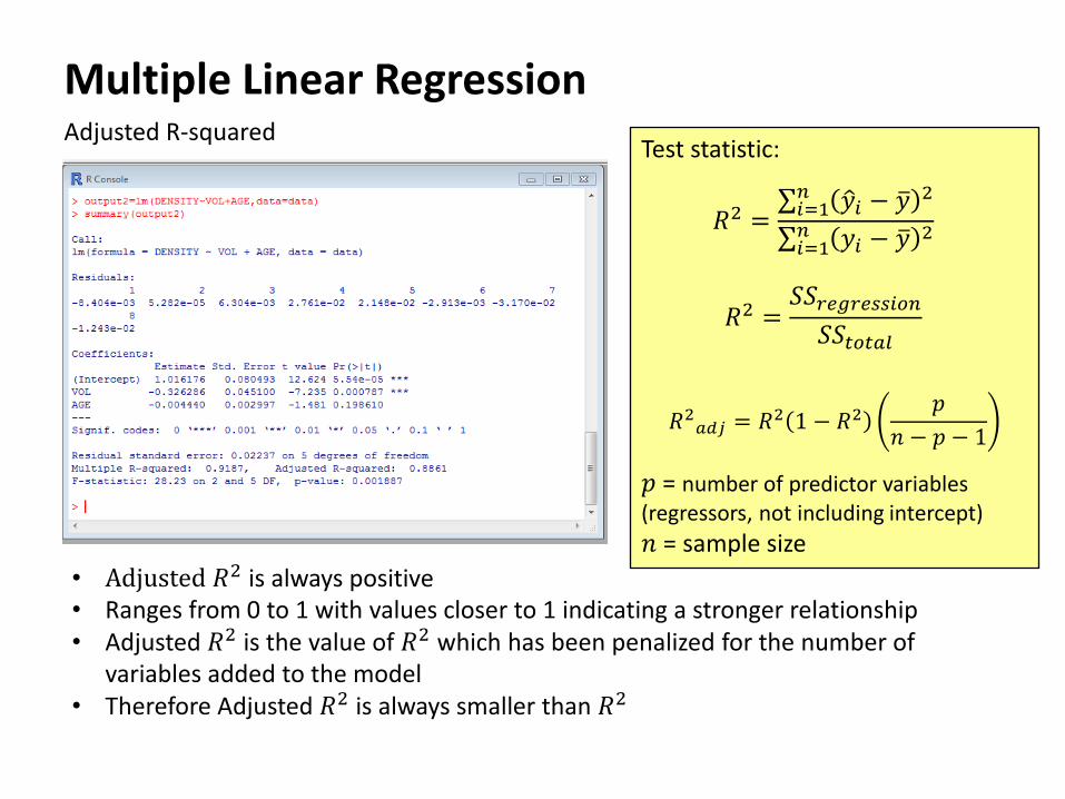
Multiple Linear Regression Adjusted R-squared

• Adjusted 𝑅2 is always positive • Ranges from 0 to 1 with values closer to 1 indicating a stronger relationship • Adjusted 𝑅2 is the value of 𝑅2 which has been penalized for the number of

variables added to the model • Therefore Adjusted 𝑅2 is always smaller than 𝑅2

Test statistic:

𝑅2𝑎𝑑𝑗 = 𝑅2 1 − 𝑅2

𝑝

𝑛 − 𝑝 − 1

𝑝 = number of predictor variables (regressors, not including intercept)

𝑛 = sample size

𝑅2 = 𝑦 𝑖 − 𝑦 2𝑛

𝑖=1

𝑦𝑖 − 𝑦 2𝑛𝑖=1

𝑅2 =𝑆𝑆𝑟𝑒𝑔𝑟𝑒𝑠𝑠𝑖𝑜𝑛

𝑆𝑆𝑡𝑜𝑡𝑎𝑙

Multiple Linear Regression Adjusted R-squared

Why do we have to Adjust 𝑅2?

For multiple linear regression there are 2 problems:

• Problem 1: Every time you add a predictor to a model, the R-squared increases, even if due to chance alone. It never decreases. Consequently, a model with more terms may appear to have a better fit simply because it has more terms.

• Problem 2: If a model has too many predictors and higher order polynomials, it begins to model the random noise in the data. This condition is known as over-fitting the model and it produces misleadingly high R-squared values and a lessened ability to make predictions.

Therefore for Multiple Linear Regression you need to report the Adjusted 𝑅2 which accounts for the number of predictors you had to added

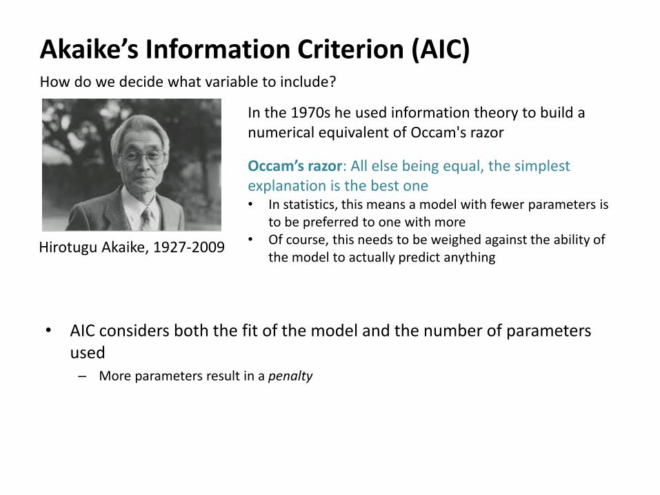
Akaike’s Information Criterion (AIC) How do we decide what variable to include?

• AIC considers both the fit of the model and the number of parameters used – More parameters result in a penalty

Hirotugu Akaike, 1927-2009

In the 1970s he used information theory to build a numerical equivalent of Occam's razor

Occam’s razor: All else being equal, the simplest explanation is the best one • In statistics, this means a model with fewer parameters is

to be preferred to one with more • Of course, this needs to be weighed against the ability of

the model to actually predict anything

Akaike’s Information Criterion (AIC)

• The model fit (AIC value) is measured ask likelihood of the parameters being correct for the population based on the observed sample

• The number of parameters is derived from the degrees of freedom that are left

• AIC value roughly equals the number of parameters minus the likelihood of the overall model – Therefore the smaller the AIC value the better the model

• Allows us to balance over- and under-fitting in our modelled relationships

– We want a model that is as simple as possible, but no simpler

– A reasonable amount of explanatory power is traded off against model size

– AIC measures the balance of this for us

How do we decide what variable to include?

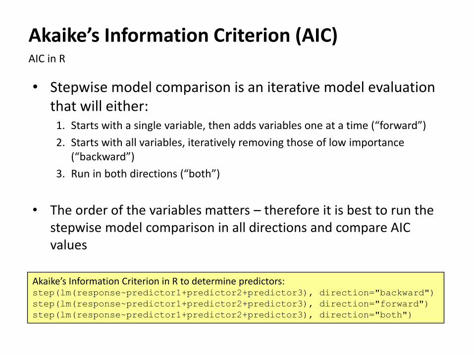
Akaike’s Information Criterion (AIC) AIC in R

Akaike’s Information Criterion in R to determine predictors: step(lm(response~predictor1+predictor2+predictor3), direction="backward")

step(lm(response~predictor1+predictor2+predictor3), direction="forward")

step(lm(response~predictor1+predictor2+predictor3), direction="both")

• Stepwise model comparison is an iterative model evaluation that will either:

1. Starts with a single variable, then adds variables one at a time (“forward”)

2. Starts with all variables, iteratively removing those of low importance (“backward”)

3. Run in both directions (“both”)

• The order of the variables matters – therefore it is best to run the stepwise model comparison in all directions and compare AIC values

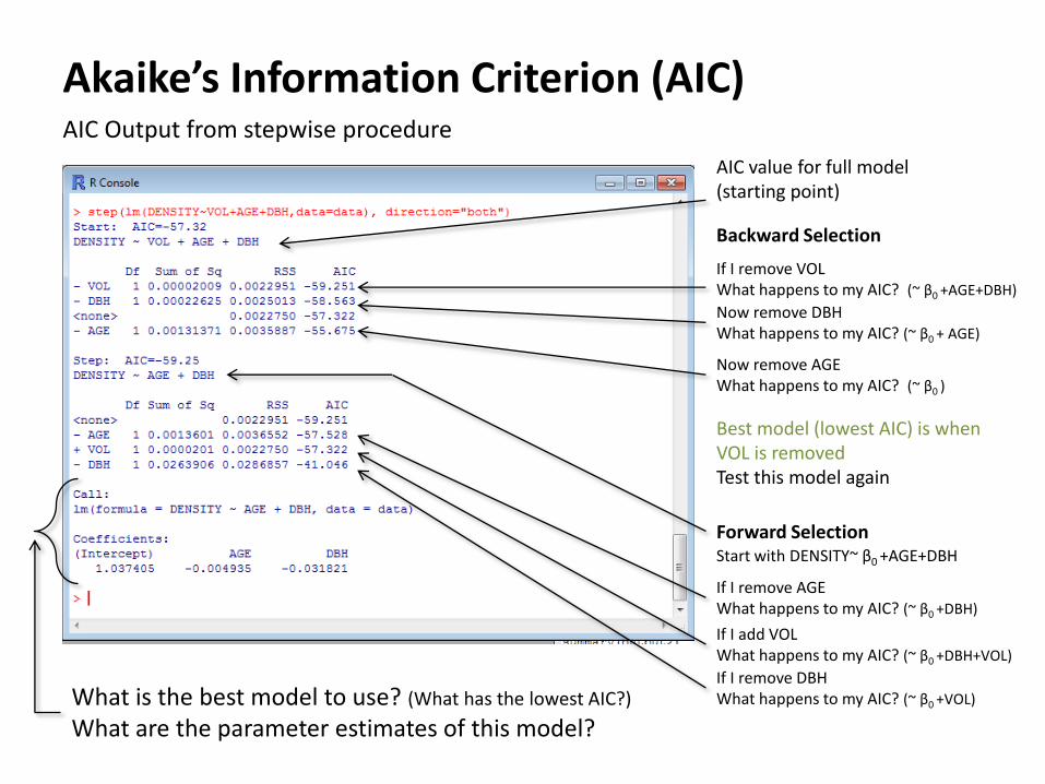
Akaike’s Information Criterion (AIC) AIC Output from stepwise procedure

AIC value for full model (starting point)

If I remove VOL What happens to my AIC? (~ β0 +AGE+DBH)

Now remove DBH What happens to my AIC? (~ β0 + AGE)

Now remove AGE What happens to my AIC? (~ β0 )

Best model (lowest AIC) is when VOL is removed Test this model again

Backward Selection

Forward Selection Start with DENSITY~ β0 +AGE+DBH

If I remove AGE What happens to my AIC? (~ β0 +DBH)

If I add VOL What happens to my AIC? (~ β0 +DBH+VOL)

If I remove DBH What happens to my AIC? (~ β0 +VOL) What is the best model to use? (What has the lowest AIC?)

What are the parameter estimates of this model?

Multiple Linear Regression Assumptions

1. For any given value of X, the distribution of Y must be normal

• BUT Y does not have to be normally distributed as a whole

2. For any given value of X, of Y must have equal variances

You can again check this by using the Shaprio Test, Bartlett Test, and residual plots on the residuals of your model What we have all ready been doing!

No assumptions for X – but be conscious of your data

Collinearity a.k.a Multicollinearity

• Occurs when predictor variables are related (linked) to one another • Meaning that one predictor can be linearly predicted from the others with a

non-trivial degree of accuracy • E.g. Climate (mean summer precipitation and heat moisture index)

• Does not reduce the predictive power or reliability of the model as a whole • BUT the coefficient estimates may change erratically in response to small

changes in the model or the data

• A model with correlated predictors CAN indicate how well the combination of predictors predicts the outcome variable • BUT it may not give valid results about any individual predictor, or about

which predictors are redundant with respect to others

Problem with predictors

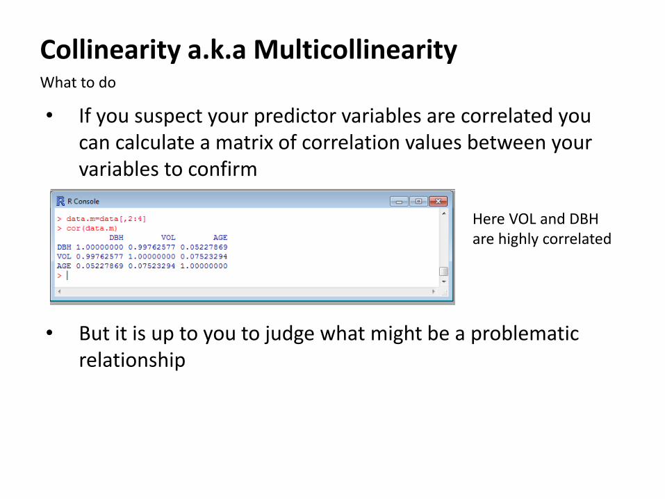
Collinearity a.k.a Multicollinearity

• If you suspect your predictor variables are correlated you can calculate a matrix of correlation values between your variables to confirm

What to do

Here VOL and DBH are highly correlated

• But it is up to you to judge what might be a problematic relationship

Collinearity a.k.a Multicollinearity What to do

• Whether or not you choose to use Multiple Regression Models depends on the question you want to answer

• Are you interested in establishing a relationship? • Are you interested in which predictors are driving that relationship?

• There are alternative techniques that can deal with highly correlated variables – these are mostly multivariate - Regression Trees = can handle correlated data well

A multiple linear relationship DOES NOT imply causation! Adjusted 𝑅2 implies a relationship rather than one or multiple factors causing another factor value Be careful of your interpretations!

Important to Remember