NASA Graduate Student Researchers Program Final … · NASA Graduate Student Researchers Program Final Report Grant Number NGT-1-02005 By Nicholas K. Borer Georgia Institute of Technology

NASA Graduate Student Researchers Program Final Report

Grant Number NGT-1-02005

By Nicholas K. Borer

Georgia Institute of Technology School of Aerospace Engineering

Atlanta, GA 30332-0150

June 2005

https://ntrs.nasa.gov/search.jsp?R=20050212117 2018-09-08T21:58:07+00:00Z

Decomposition-Based Decision Making for Aerospace Vehicle Design

Research Summary for NASA Graduate Student Researchers

Program Final Report

By Nicholas K. Borer

ii

Decomposition-Based Decision Making for Aerospace Vehicle Design

Thesis Advisory Committee Dr. Dimitri Mavris, GT/AE, Thesis Advisor Dr. Daniel Schrage, GT/AE Dr. Alan Wilhite, GT/AE, National Institute of Aerospace Mr. Craig Nickol, NASA Langley Research Center Abstract Most practical engineering systems design problems have multiple and conflicting objectives. Furthermore, the satisfactory attainment level for each objective (“requirement”) is likely uncertain early in the design process. Systems with long design cycle times will exhibit more of this uncertainty throughout the design process. This is further complicated if the system is expected to perform for a relatively long period of time, as now it will need to grow as new requirements are identified and new technologies are introduced. These points identify a need for a systems design technique that enables decision making amongst multiple objectives in the presence of uncertainty. Traditional design techniques deal with a single objective or a small number of objectives that are often aggregates of the overarching goals sought through the generation of a new system. Other requirements, although uncertain, are viewed as static constraints to this single or multiple objective optimization problem. With either of these formulations, enabling tradeoffs between the requirements, objectives, or combinations thereof is a slow, serial process that becomes increasingly complex as more criteria are added. This research proposal outlines a technique that attempts to address these and other idiosyncrasies associated with modern aerospace systems design. The proposed formulation first recasts systems design into a multiple criteria decision making problem. The now multiple objectives are decomposed to discover the critical characteristics of the objective space. Tradeoffs between the objectives are considered amongst these critical characteristics by comparison to a probabilistic ideal tradeoff solution. The proposed formulation represents a radical departure from traditional methods. A pitfall of this technique is in the validation of the solution: in a multi-objective sense, how can a decision maker justify a choice between non-dominated alternatives? A series of examples help the reader to observe how this technique can be applied to aerospace systems design and compare the results of this so-called Decomposition-Based Decision Making to more traditional design approaches.

TABLE OF CONTENTS

LIST OF TABLES . . . . . . . . . . . . . . . . . . . . . . . . . . . . . . . . . . . v

LIST OF FIGURES . . . . . . . . . . . . . . . . . . . . . . . . . . . . . . . . . . vi

I INTRODUCTION . . . . . . . . . . . . . . . . . . . . . . . . . . . . . . . . . 1

1.1 Motivation . . . . . . . . . . . . . . . . . . . . . . . . . . . . . . . . . . . . 1

1.1.1 Multi-Mission Sizing . . . . . . . . . . . . . . . . . . . . . . . . . . 2

1.1.2 Requirements Uncertainty . . . . . . . . . . . . . . . . . . . . . . . 3

II REQUIREMENTS AND AIRCRAFT SIZING . . . . . . . . . . . . . . . 5

2.1 The Engineering Design Process . . . . . . . . . . . . . . . . . . . . . . . . 5

2.1.1 Requirements Specification . . . . . . . . . . . . . . . . . . . . . . . 7

2.2 Traditional Single-Objective Approaches . . . . . . . . . . . . . . . . . . . 8

2.3 Modern Sizing Methods . . . . . . . . . . . . . . . . . . . . . . . . . . . . . 9

2.3.1 Multidisciplinary Design Optimization and Statistical Techniques . 9

2.3.2 Evolving Techniques . . . . . . . . . . . . . . . . . . . . . . . . . . 12

2.4 Multi-Mission Approaches . . . . . . . . . . . . . . . . . . . . . . . . . . . 12

2.4.1 Shortfalls . . . . . . . . . . . . . . . . . . . . . . . . . . . . . . . . . 13

2.4.2 Requirements Fitting for Multi-Mission Design . . . . . . . . . . . 13

III DESIGN AND DECISION MAKING . . . . . . . . . . . . . . . . . . . . 14

3.1 Pareto Optimality . . . . . . . . . . . . . . . . . . . . . . . . . . . . . . . . 15

3.2 Axiomatic Design . . . . . . . . . . . . . . . . . . . . . . . . . . . . . . . . 16

3.3 Multiple Criteria Decision Making Techniques . . . . . . . . . . . . . . . . 17

3.3.1 The Ideal Solution . . . . . . . . . . . . . . . . . . . . . . . . . . . 17

3.3.2 Simple Additive Weighting . . . . . . . . . . . . . . . . . . . . . . . 19

3.3.3 TOPSIS . . . . . . . . . . . . . . . . . . . . . . . . . . . . . . . . . 20

3.3.4 Compromise Programming . . . . . . . . . . . . . . . . . . . . . . . 22

3.3.5 MCDM for Systems Design . . . . . . . . . . . . . . . . . . . . . . 23

3.4 Case Study: Notional Multi-Role Fighter . . . . . . . . . . . . . . . . . . . 23

3.4.1 Problem Formulation . . . . . . . . . . . . . . . . . . . . . . . . . . 24

3.4.2 Results and Implications . . . . . . . . . . . . . . . . . . . . . . . . 26

iii

3.4.3 Research Directions . . . . . . . . . . . . . . . . . . . . . . . . . . . 27

IV DECISION MAKING FOR LARGE-SCALE PROBLEMS . . . . . . . 28

4.1 Generalized Probabilistic MCDM Formulation . . . . . . . . . . . . . . . . 28

4.1.1 Generating Alternatives . . . . . . . . . . . . . . . . . . . . . . . . 29

4.2 MCDM Example Problem: Beam Design . . . . . . . . . . . . . . . . . . . 30

4.2.1 Beam Analysis and Design Procedure . . . . . . . . . . . . . . . . . 33

4.2.2 Initial Results . . . . . . . . . . . . . . . . . . . . . . . . . . . . . . 35

4.3 Weighting Schemes . . . . . . . . . . . . . . . . . . . . . . . . . . . . . . . 37

4.3.1 Entropy-Based Weights . . . . . . . . . . . . . . . . . . . . . . . . . 37

4.3.2 Constraint and Threshold Modeling . . . . . . . . . . . . . . . . . . 40

4.3.3 Beam Design Problem with Dynamic Importance Weighting . . . . 42

4.4 Requirements Decomposition . . . . . . . . . . . . . . . . . . . . . . . . . . 45

4.4.1 Decomposition Techniques for Linear Systems . . . . . . . . . . . . 46

4.4.2 Singular Value Decomposition for Response Surface Equations . . . 47

4.4.3 Decision Making with Characteristic Requirements . . . . . . . . . 50

4.4.4 Requirements Grouping . . . . . . . . . . . . . . . . . . . . . . . . 51

4.5 Decomposition-Based Decision Making . . . . . . . . . . . . . . . . . . . . 53

4.5.1 Results for Beam Design Problem . . . . . . . . . . . . . . . . . . . 53

4.6 Directions for Large-Scale Decision Making . . . . . . . . . . . . . . . . . . 57

REFERENCES . . . . . . . . . . . . . . . . . . . . . . . . . . . . . . . . . . . . . 58

iv

LIST OF TABLES

1 Notional Multi-Role Fighter Missions . . . . . . . . . . . . . . . . . . . . . . 24

2 Notional Multi-Role Fighter Decision Metrics . . . . . . . . . . . . . . . . . 25

3 Single and Multi-Objective Results for Beam Design Problem . . . . . . . . 35

4 Entropy-Based Weights Generated for Beam Design Problem . . . . . . . . 39

5 Ranges of Requirements for Beam Design Problem . . . . . . . . . . . . . . 39

6 Modified Entropy-Based Weights for Beam Design Problem Considering Thresh-old Values . . . . . . . . . . . . . . . . . . . . . . . . . . . . . . . . . . . . . 40

7 Compromise Programming Results for Beam Design Problem with DynamicWeights . . . . . . . . . . . . . . . . . . . . . . . . . . . . . . . . . . . . . . 45

8 Third-Order Normalized Response Surface Equation Coefficients for BeamDesign Problem . . . . . . . . . . . . . . . . . . . . . . . . . . . . . . . . . . 48

9 Recomposition Coefficient Matrix for Beam Design Problem . . . . . . . . . 50

10 Vector Angles of Requirements for Beam Design Problem . . . . . . . . . . 52

11 DBDM Results for Beam Problem Scaled by Singular Values . . . . . . . . 55

12 Unscaled DBDM Results for Beam Problem . . . . . . . . . . . . . . . . . . 55

13 DBDM Results for Beam Problem with Varying Critical Characteristics Scaledby Singular Values . . . . . . . . . . . . . . . . . . . . . . . . . . . . . . . . 56

14 Unscaled DBDM Results with Varying Critical Characteristics for BeamProblem . . . . . . . . . . . . . . . . . . . . . . . . . . . . . . . . . . . . . . 56

v

LIST OF FIGURES

1 Carrier Air Wing Composition . . . . . . . . . . . . . . . . . . . . . . . . . 2

2 The Engineering Design Process . . . . . . . . . . . . . . . . . . . . . . . . 6

3 The Systems Engineering Process . . . . . . . . . . . . . . . . . . . . . . . . 6

4 Sample Design Structure Matrix . . . . . . . . . . . . . . . . . . . . . . . . 10

5 Probabilistic Decision Making . . . . . . . . . . . . . . . . . . . . . . . . . . 11

6 Two-Dimensional Pareto Frontier . . . . . . . . . . . . . . . . . . . . . . . . 15

7 Axiomatic Faucet Design . . . . . . . . . . . . . . . . . . . . . . . . . . . . 16

8 A Taxonomy of Methods for Multiple Attribute Decision Making . . . . . . 18

9 A Taxonomy of Methods for Multiple Objective Decision Making . . . . . . 18

10 Positive and Negative Ideal Solutions from Several Alternatives . . . . . . . 19

11 SAW Indifference Curves Projected Onto Non-Convex Pareto Frontier . . . 20

12 TOPSIS Solutions for Two Non-Convex Pareto Frontiers . . . . . . . . . . . 21

13 Compromise Programming Solutions for Different Values of p . . . . . . . . 23

14 Notional Multi-Role Fighter Problem Formulation and Execution . . . . . . 26

15 Nondominated Population Fraction for Increasing Number of Objectives . . 30

16 Pertinent Dimensions and Material Properties of Beam Design Problem . . 31

17 Loading Conditions for Beam Design Problem . . . . . . . . . . . . . . . . . 31

18 Surrogate Models of Beam Requirements . . . . . . . . . . . . . . . . . . . . 34

19 Actual versus Predicted Results for Surrogate Models . . . . . . . . . . . . 34

20 Objective Function of Compromise Programming Solution to Six-RequirementBeam Design Problem . . . . . . . . . . . . . . . . . . . . . . . . . . . . . . 36

21 Objective Function of Compromise Programming Solution to Eight-RequirementBeam Design Problem . . . . . . . . . . . . . . . . . . . . . . . . . . . . . . 36

22 Example Dynamic Weight Variation with yj(~x) . . . . . . . . . . . . . . . . 42

23 Variation of Weights for Beam Design Problem with yj(~x) . . . . . . . . . . 43

24 Objective Function for Six-Requirement Beam Design Problem with DynamicWeights . . . . . . . . . . . . . . . . . . . . . . . . . . . . . . . . . . . . . . 44

25 Objective Function for Eight-Requirement Beam Design Problem with Dy-namic Weights . . . . . . . . . . . . . . . . . . . . . . . . . . . . . . . . . . 44

26 Singular Values and Coefficients of Characteristic Requirements for BeamDesign Problem . . . . . . . . . . . . . . . . . . . . . . . . . . . . . . . . . . 49

vi

27 Flowchart for Decomposition-Based Decision Making . . . . . . . . . . . . . 54

vii

CHAPTER I

INTRODUCTION

Most practical engineering systems design problems have multiple and conflicting objectives.Furthermore, the satisfactory attainment level for each objective (“requirement”) is likelyuncertain early in the design process. Systems with long design cycle times will exhibitmore of this uncertainty throughout the design process. This is further complicated if thesystem is expected to perform for a relatively long period of time, as now it will needto grow as new requirements are identified and new technologies are introduced. Thesepoints identify a need for a systems design technique that enables decision making amongstmultiple objectives in the presence of uncertainty.

Traditional design techniques deal with a single objective or only a few objectives thatare often aggregates of the overarching goals sought through the generation of a new system.Other requirements, although uncertain, are viewed as static constraints to this single- ormulti-objective optimization problem. With this formulation, enabling tradeoffs amongstthe requirements, objectives, or combinations thereof is a slow, serial process that becomesincreasingly complex as more criteria are added.

The research in this document outlines a technique that attempts to address these andother idiosyncracies associated with modern aerospace systems design. The proposed for-mulation first recasts systems design into a fully multiple criteria decision making problem.The now multiple objectives are decomposed to discover the critical characteristics of theobjective space. Tradeoffs amongst the objectives are considered amongst these criticalcharacteristics by comparison to a probabilistic ideal tradeoff solution.

The proposed formulation represents a radical departure from traditional methods. Apitfall of this technique is in the validation of the solution: in a multi-objective sense, howcan a decision maker justify a choice between non-dominated alternatives? A series ofexamples help the reader to get a feel for how this technique can be applied to aerospacesystems design and compare the results of this so-called Decomposition-Based DecisionMaking to more traditional design approaches.

1.1 Motivation

The motivation for this research began with the author’s involvement in a first-year graduatedesign competition involving a multi-mission aircraft. This competition required the designteam to determine the salient characteristics of a vehicle with multiple, conflicting missionrequirements and subsequently to design an aircraft to these features. The identificationof these features followed an analysis of the vehicle’s “mission space” to determine whichrequirements would be the design drivers [Mavris and Borer, 2001].

This first approach at multi-mission sizing represented a technique that is most typicalof modern multi-mission vehicle design; that is, to design the aircraft to only the moststringent requirements. Though effective, it does little to accommodate tradeoffs and canquickly result in an infeasible design. If nothing else, this initial design project broached twosubject areas critical to the development of a new technique: the need for a multi-missionsizing method and for the ability to capture uncertainty in requirements specification.

1

1.1.1 Multi-Mission Sizing

The first 11 seconds of manned heavier-than-air flight began on 17 December 1903, nowover a century ago. Since those first flights off the dunes of Kill Devil Hills, aircraft haveevolved into massive, complex, and versatile machines. The first practical use of aircraft forcarrying passengers or cargo was realized within a decade, and its military applications forobservation and attack soon after. By the fourth decade of powered flight aircraft were usedfor a variety of missions: cargo and troop transport, precision bombing, aerial photography,escort, interception, and many others. By the end of the sixth decade of powered flightmanufacturers were building aircraft for every conceivable mission.

However, as the number of missions for aircraft increased, manufacturers and operatorsfound that production and operations costs increased and tactical redundancy suffered. Thisproblem was compounded as advances in technology required a wider array of missions, suchas supersonic attack, airborne early warning, and electronic surveillance. Certain aircraftwere tasked with synergistic missions in an effort to alleviate these problems.

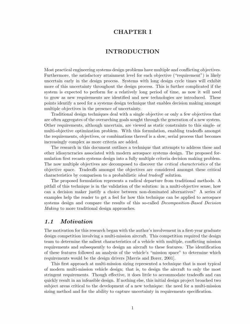
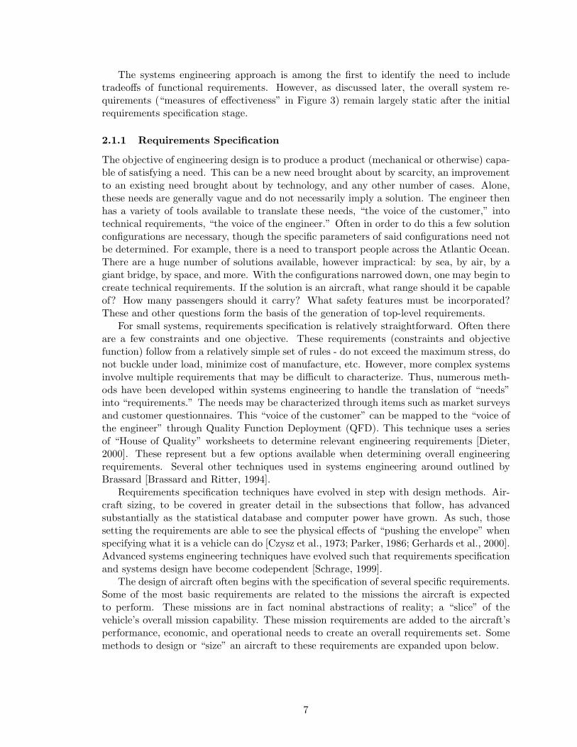
The notion of the multi-role aircraft, though not new, has seen increased emphasis overthe years. This trend, though difficult to explicitly document, can be exemplified in thecomposition of aircraft carrier air wings. Figure 1 compares the number of different types ofaircraft aboard an aircraft carrier versus the number of missions performed by these aircraftfor different historical periods, compiled from several different resources [Department of theNavy, 2005; Federation of American Scientists, 2005; Toppan, 2003].

3

8

23

26 26 26 26

3

89

8 87

6

0

5

10

15

20

25

30

1942 1952 1970 1983 1991 1996 2004Year

number of missions number of aircraft types

Figure 1: Carrier Air Wing Composition

This figure shows that the number of missions has climbed rapidly and levelled off withrespect to aircraft carrier operations, yet the number of different aircraft types saw a shortincrease followed by a steady decrease. The carrier air wing of the future will deploy even

2

fewer craft as new programs such as the multi-mission capable F/A-18E and F-35C aircraftenter service and replace aging airframes [Young et al., 1998; Sherman and Hardiman, 2003].

The increased emphasis of multi-role capability for aircraft can be traced to two principalreasons: affordability and redundancy. Employing a single aircraft type or variant of saidtype for several roles reduces the need for specialized equipment, personnel, training, andspare parts, among other resources. It also enables economies of scale through larger-scale mass-production of the same airframe. All of these attributes point to a reduction inoverall life-cycle costs at tactical (and higher) levels. Redundancy is increased for many ofthe same reasons. As an example, consider two squadrons: one with 10 dedicated attackand 10 dedicated fighter aircraft, and one with 20 multi-role fighters. If five aircraft arelost on a fighter mission, the squadron with dedicated aircraft exhibits a 50% loss in fightercapability, while the multi-role squadron can spread that loss out evenly over its attackand fighter capability as needed. This is important not only in military applications butalso civil applications as many passenger air carriers begin to investigate the feasibility ofintermodal (passenger by day, cargo by night) transports [Nelson et al., 2001].

Unfortunately, multi-mission capability comes at a price. One maxim in aerospace de-sign is that every additional requirement imposed on a system will compromise the designin some way. This concept of “no free lunch” will manifest itself as a decrease in effec-tiveness in another requirement, such as a performance or vehicle-level cost measure. Theonly exception to this rule is in the trivial case of a completely dominated or redundantrequirement, in which case the true multi-role capability of the system is not expanded.

1.1.2 Requirements Uncertainty

Successful design of any system begins with specification of requirements. These require-ments are composed of one or more objectives and zero to many constraints. As aerospacevehicle design has progressed, the requirements imposed on vehicles have become morenumerous and stringent. Requirements are influenced by advances in technology, the envi-ronment, politics, and many other factors.

Most engineering problem solving techniques begin with a static set of requirements.Any change to these requirements can change what was once the best solution to a dif-ferent solution. As design cycle times increase, there is a larger chance that the variousfactors shaping the requirements will change as well, thus resulting in changes to the orig-inal requirements. This can have a substantial effect on modern aerospace vehicle design.To compare design cycle times, consider that the Lockheed P-80 Shooting Star, the firstoperational jet fighter made in the United States, went from drawing board to first flight in143 days [Rich and Janos, 1994]. Compare this to a modern jet fighter, the F-22 Raptor.The Raptor itself was conceived in 1983 and first flew in 1997, and as of this writing in 2005the first squadron is becoming operational. This example, though radical, exemplifies theincrease in design cycle time: 143 days to 14 years! Even in this vein, one must considerthat the original requirements for the F-22 date back to the Advanced Tactical Fighterconcept first proposed in 1971 [Piccirillo, 1998]. Over that time numerous changes havebeen seen in the technological environment (stealth), political environment (the fall of theUSSR), and the fiscal environment, to name a few.

Further complicating requirements specification is the concept of growth potential.Aerospace vehicles, at their extraordinary expense and complexity, are expected to per-form for a relatively long period of time. Over this time the operational environment andassociated requirements will change. Commercial operators will be faced with a different

3

market, more stringent environmental regulations, and safety regulations. Military opera-tors will face new enemies and weapons systems. Overall, a successful aircraft will need tohave the ability to grow and change throughout its life cycle. Compare the service of theB-52 subsonic strategic bomber to that of the B-58 supersonic bomber: both were contem-poraries; the earliest operational B-52 first flew in 1955 and the B-58 in 1960. The latestmodels of both aircraft were produced in 1962. However, the B-52 is so effective, affordable,and adaptable for strategic bombing that it is planned to remain in service until 2040, 85years after the first model and 78 years after the last of the current models entered service!The B-58 only lasted until 1970, 10 years after entering service simply because it was notnearly as versatile or adaptable in its future environment [Baugher, 2005; Federation ofAmerican Scientists, 2005].

These all point to another maxim related to aerospace vehicle design: The requirementsspecified for the system today will be different than those faced at the beginning of its oper-ational life, which will further change throughout the system’s entire life cycle.

4

CHAPTER II

REQUIREMENTS AND AIRCRAFT SIZING

The bases of multi-mission sizing have to do with the broader spectrum of systems de-sign methods and requirements specification. Therefore, to gain an appreciation of theissues associated with multi-mission sizing one must first understand the idiosyncracies as-sociated with the engineering design process, requirements specification, and vehicle sizingmethodologies. Each of these areas has evolved over the years to take advantage of a largerbody of knowledge and better resources to tackle these various problems. What followsis an overview of the origins and growth experienced in these fields, though the reader iscautioned that this is by no means a comprehensive review.

2.1 The Engineering Design Process

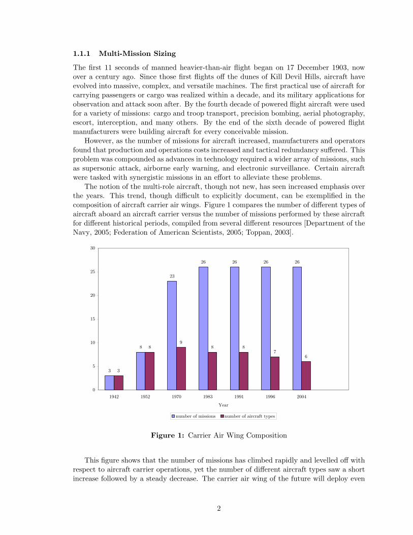
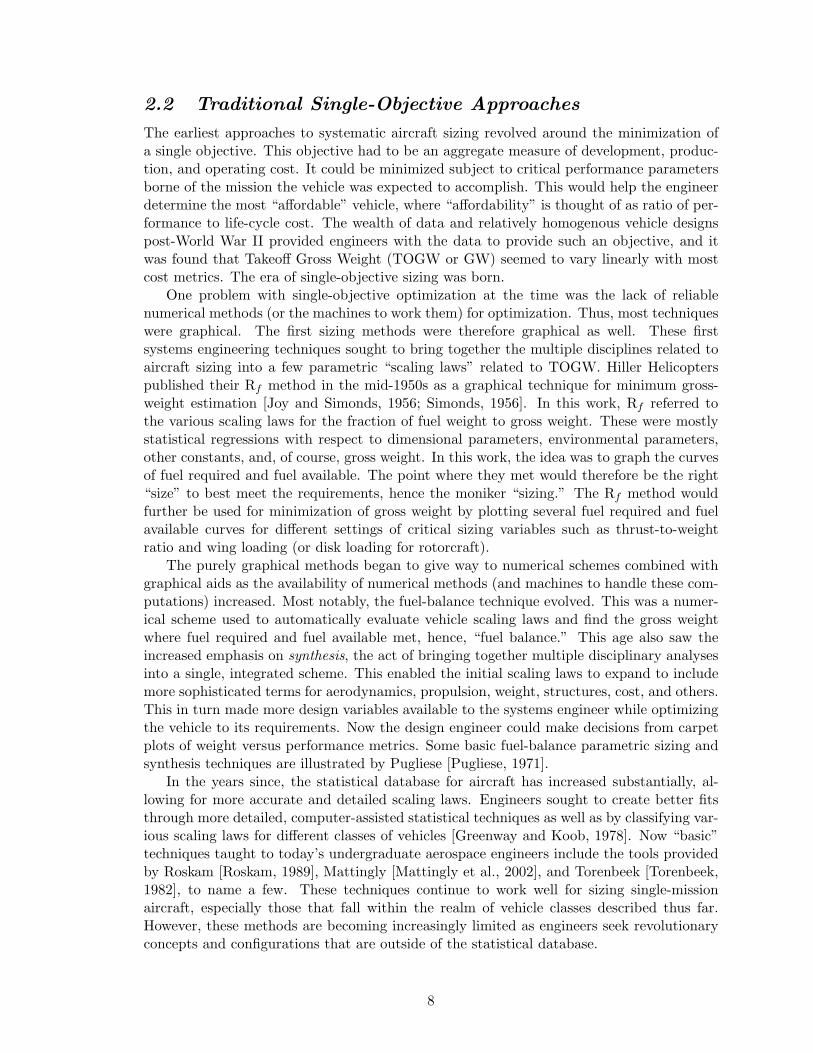
Several models exist for the engineering design process related to aerospace vehicles. Raymersuggests a serial, three-tiered process of conceptual design, preliminary design, and detaildesign, with requirements feeding into the conceptual design process and fabrication fol-lowing detail design [Raymer, 1999]. This text, meant as a single source for undergraduateengineering students, presents a deliberately simplified process. More rigorous techniquesinvolve more stages, such as detailed requirements generation studies and considerations ofthe entire life cycle of the vehicle. Asimow enumerates an eight-phase design process toembody all of these concepts, from feasibility studies to planning for retirement [Asimow,1962]. Dieter revives and modernizes these concepts in his text on systems design [Dieter,2000]. Of particular interest are the initial phases of what Dieter refers to as conceptualdesign and embodiment design. This refined design process is illustrated in Figure 2.

The life-cycle approach to engineering design is imbedded into the concept of systemsengineering. The Defense Systems Management College [Leonard, 1999] defines systemsengineering as:

. . . an interdisciplinary engineering management process to evolve and verifyan integrated, life cycle balanced set of system solutions that satisfy customerneeds.

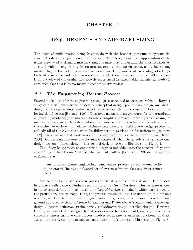
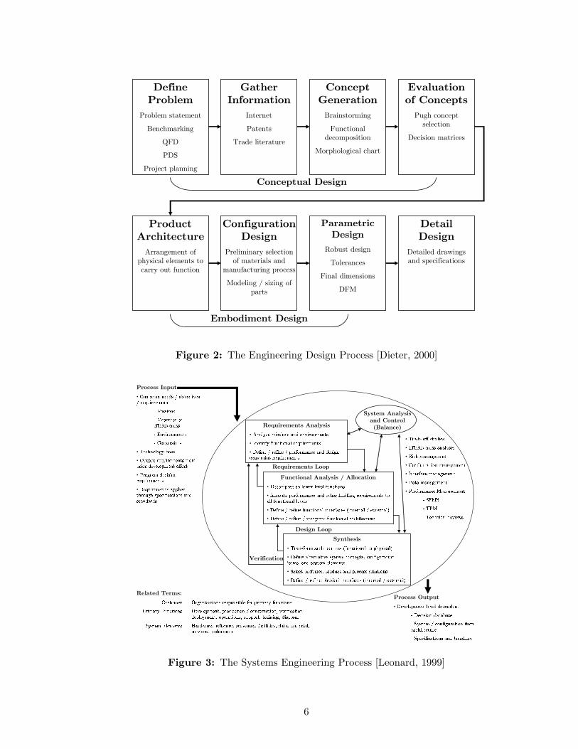
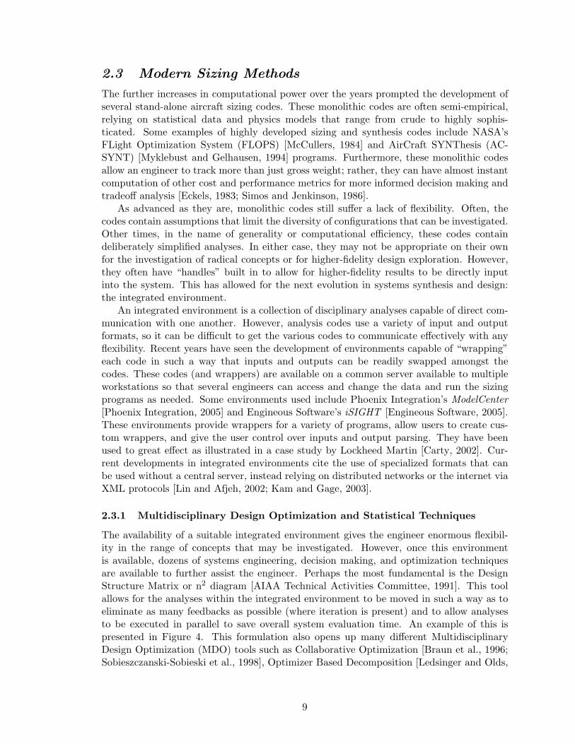
The text further discusses four phases in the development of a design. The processfirst starts with concept studies, resulting in a functional baseline. This baseline is usedin the system definition phase until an allocated baseline is defined, which carries over tothe preliminary design stage. Here, the process continues until the definition of a productbaseline, used in the final detail design phases. In general, these phases follow the samegeneral approach as those reference by Raymer and Dieter above (requirements, conceptualdesign / system definition, preliminary / embodiment design, detailed design). However,the Department of Defense greatly elaborates on methods for identifying requirements forsystems engineering. The core process involves requirements analysis, functional analysis,system synthesis, and system analysis and control. This process is illustrated in Figure 3.

5

Define Problem

Problem statementBenchmarking

QFDPDS

Project planning

Gather Information

InternetPatents

Trade literature

Concept GenerationBrainstormingFunctional

decompositionMorphological chart

Evaluation of Concepts

Pugh concept selection

Decision matrices

Product Architecture

Arrangement of physical elements to carry out function

Configuration Design

Preliminary selection of materials and

manufacturing processModeling / sizing of

parts

Parametric Design

Robust designTolerances

Final dimensionsDFM

Detail Design

Detailed drawings and specifications

Conceptual Design

Embodiment Design

Figure 2: The Engineering Design Process [Dieter, 2000]

Process Input•��

��

��

��

��

• ��

• ��

• ��

• ��

Requirements Analysis• ��

• !��

• "��

Functional Analysis / Allocation• "� ��#��

• ��

• "�� $��%��&

• "��

Synthesis• �� $�� &

• "�� ' ��'��

• (��

• "�� $��%��&

System Analysis and Control (Balance)

Process Output• "��

�"� ��

�(��

�(��

• ��

• ��

• ��)��

•��

• !��

• "��

• ��

�(��(�� #�

Related Terms:��*

��+�� *

(��*

��

"��'�� '�� '��'��'��'��'��,��#��'��#��'��'�� '��'��'�� '��

Verification

Design Loop

Requirements Loop

Figure 3: The Systems Engineering Process [Leonard, 1999]

6

The systems engineering approach is among the first to identify the need to includetradeoffs of functional requirements. However, as discussed later, the overall system re-quirements (“measures of effectiveness” in Figure 3) remain largely static after the initialrequirements specification stage.

2.1.1 Requirements Specification

The objective of engineering design is to produce a product (mechanical or otherwise) capa-ble of satisfying a need. This can be a new need brought about by scarcity, an improvementto an existing need brought about by technology, and any other number of cases. Alone,these needs are generally vague and do not necessarily imply a solution. The engineer thenhas a variety of tools available to translate these needs, “the voice of the customer,” intotechnical requirements, “the voice of the engineer.” Often in order to do this a few solutionconfigurations are necessary, though the specific parameters of said configurations need notbe determined. For example, there is a need to transport people across the Atlantic Ocean.There are a huge number of solutions available, however impractical: by sea, by air, by agiant bridge, by space, and more. With the configurations narrowed down, one may begin tocreate technical requirements. If the solution is an aircraft, what range should it be capableof? How many passengers should it carry? What safety features must be incorporated?These and other questions form the basis of the generation of top-level requirements.

For small systems, requirements specification is relatively straightforward. Often thereare a few constraints and one objective. These requirements (constraints and objectivefunction) follow from a relatively simple set of rules - do not exceed the maximum stress, donot buckle under load, minimize cost of manufacture, etc. However, more complex systemsinvolve multiple requirements that may be difficult to characterize. Thus, numerous meth-ods have been developed within systems engineering to handle the translation of “needs”into “requirements.” The needs may be characterized through items such as market surveysand customer questionnaires. This “voice of the customer” can be mapped to the “voice ofthe engineer” through Quality Function Deployment (QFD). This technique uses a seriesof “House of Quality” worksheets to determine relevant engineering requirements [Dieter,2000]. These represent but a few options available when determining overall engineeringrequirements. Several other techniques used in systems engineering around outlined byBrassard [Brassard and Ritter, 1994].

Requirements specification techniques have evolved in step with design methods. Air-craft sizing, to be covered in greater detail in the subsections that follow, has advancedsubstantially as the statistical database and computer power have grown. As such, thosesetting the requirements are able to see the physical effects of “pushing the envelope” whenspecifying what it is a vehicle can do [Czysz et al., 1973; Parker, 1986; Gerhards et al., 2000].Advanced systems engineering techniques have evolved such that requirements specificationand systems design have become codependent [Schrage, 1999].

The design of aircraft often begins with the specification of several specific requirements.Some of the most basic requirements are related to the missions the aircraft is expectedto perform. These missions are in fact nominal abstractions of reality; a “slice” of thevehicle’s overall mission capability. These mission requirements are added to the aircraft’sperformance, economic, and operational needs to create an overall requirements set. Somemethods to design or “size” an aircraft to these requirements are expanded upon below.

7

2.2 Traditional Single-Objective Approaches

The earliest approaches to systematic aircraft sizing revolved around the minimization ofa single objective. This objective had to be an aggregate measure of development, produc-tion, and operating cost. It could be minimized subject to critical performance parametersborne of the mission the vehicle was expected to accomplish. This would help the engineerdetermine the most “affordable” vehicle, where “affordability” is thought of as ratio of per-formance to life-cycle cost. The wealth of data and relatively homogenous vehicle designspost-World War II provided engineers with the data to provide such an objective, and itwas found that Takeoff Gross Weight (TOGW or GW) seemed to vary linearly with mostcost metrics. The era of single-objective sizing was born.

One problem with single-objective optimization at the time was the lack of reliablenumerical methods (or the machines to work them) for optimization. Thus, most techniqueswere graphical. The first sizing methods were therefore graphical as well. These firstsystems engineering techniques sought to bring together the multiple disciplines related toaircraft sizing into a few parametric “scaling laws” related to TOGW. Hiller Helicopterspublished their Rf method in the mid-1950s as a graphical technique for minimum gross-weight estimation [Joy and Simonds, 1956; Simonds, 1956]. In this work, Rf referred tothe various scaling laws for the fraction of fuel weight to gross weight. These were mostlystatistical regressions with respect to dimensional parameters, environmental parameters,other constants, and, of course, gross weight. In this work, the idea was to graph the curvesof fuel required and fuel available. The point where they met would therefore be the right“size” to best meet the requirements, hence the moniker “sizing.” The Rf method wouldfurther be used for minimization of gross weight by plotting several fuel required and fuelavailable curves for different settings of critical sizing variables such as thrust-to-weightratio and wing loading (or disk loading for rotorcraft).

The purely graphical methods began to give way to numerical schemes combined withgraphical aids as the availability of numerical methods (and machines to handle these com-putations) increased. Most notably, the fuel-balance technique evolved. This was a numer-ical scheme used to automatically evaluate vehicle scaling laws and find the gross weightwhere fuel required and fuel available met, hence, “fuel balance.” This age also saw theincreased emphasis on synthesis, the act of bringing together multiple disciplinary analysesinto a single, integrated scheme. This enabled the initial scaling laws to expand to includemore sophisticated terms for aerodynamics, propulsion, weight, structures, cost, and others.This in turn made more design variables available to the systems engineer while optimizingthe vehicle to its requirements. Now the design engineer could make decisions from carpetplots of weight versus performance metrics. Some basic fuel-balance parametric sizing andsynthesis techniques are illustrated by Pugliese [Pugliese, 1971].

In the years since, the statistical database for aircraft has increased substantially, al-lowing for more accurate and detailed scaling laws. Engineers sought to create better fitsthrough more detailed, computer-assisted statistical techniques as well as by classifying var-ious scaling laws for different classes of vehicles [Greenway and Koob, 1978]. Now “basic”techniques taught to today’s undergraduate aerospace engineers include the tools providedby Roskam [Roskam, 1989], Mattingly [Mattingly et al., 2002], and Torenbeek [Torenbeek,1982], to name a few. These techniques continue to work well for sizing single-missionaircraft, especially those that fall within the realm of vehicle classes described thus far.However, these methods are becoming increasingly limited as engineers seek revolutionaryconcepts and configurations that are outside of the statistical database.

8

2.3 Modern Sizing Methods

The further increases in computational power over the years prompted the development ofseveral stand-alone aircraft sizing codes. These monolithic codes are often semi-empirical,relying on statistical data and physics models that range from crude to highly sophis-ticated. Some examples of highly developed sizing and synthesis codes include NASA’sFLight Optimization System (FLOPS) [McCullers, 1984] and AirCraft SYNThesis (AC-SYNT) [Myklebust and Gelhausen, 1994] programs. Furthermore, these monolithic codesallow an engineer to track more than just gross weight; rather, they can have almost instantcomputation of other cost and performance metrics for more informed decision making andtradeoff analysis [Eckels, 1983; Simos and Jenkinson, 1986].

As advanced as they are, monolithic codes still suffer a lack of flexibility. Often, thecodes contain assumptions that limit the diversity of configurations that can be investigated.Other times, in the name of generality or computational efficiency, these codes containdeliberately simplified analyses. In either case, they may not be appropriate on their ownfor the investigation of radical concepts or for higher-fidelity design exploration. However,they often have “handles” built in to allow for higher-fidelity results to be directly inputinto the system. This has allowed for the next evolution in systems synthesis and design:the integrated environment.

An integrated environment is a collection of disciplinary analyses capable of direct com-munication with one another. However, analysis codes use a variety of input and outputformats, so it can be difficult to get the various codes to communicate effectively with anyflexibility. Recent years have seen the development of environments capable of “wrapping”each code in such a way that inputs and outputs can be readily swapped amongst thecodes. These codes (and wrappers) are available on a common server available to multipleworkstations so that several engineers can access and change the data and run the sizingprograms as needed. Some environments used include Phoenix Integration’s ModelCenter[Phoenix Integration, 2005] and Engineous Software’s iSIGHT [Engineous Software, 2005].These environments provide wrappers for a variety of programs, allow users to create cus-tom wrappers, and give the user control over inputs and output parsing. They have beenused to great effect as illustrated in a case study by Lockheed Martin [Carty, 2002]. Cur-rent developments in integrated environments cite the use of specialized formats that canbe used without a central server, instead relying on distributed networks or the internet viaXML protocols [Lin and Afjeh, 2002; Kam and Gage, 2003].

2.3.1 Multidisciplinary Design Optimization and Statistical Techniques

The availability of a suitable integrated environment gives the engineer enormous flexibil-ity in the range of concepts that may be investigated. However, once this environmentis available, dozens of systems engineering, decision making, and optimization techniquesare available to further assist the engineer. Perhaps the most fundamental is the DesignStructure Matrix or n2 diagram [AIAA Technical Activities Committee, 1991]. This toolallows for the analyses within the integrated environment to be moved in such a way as toeliminate as many feedbacks as possible (where iteration is present) and to allow analysesto be executed in parallel to save overall system evaluation time. An example of this ispresented in Figure 4. This formulation also opens up many different MultidisciplinaryDesign Optimization (MDO) tools such as Collaborative Optimization [Braun et al., 1996;Sobieszczanski-Sobieski et al., 1998], Optimizer Based Decomposition [Ledsinger and Olds,

9

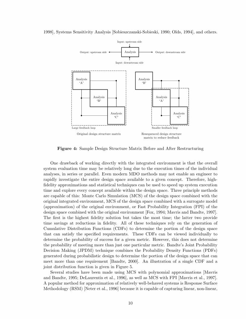
1998], Systems Sensitivity Analysis [Sobieszczanski-Sobieski, 1990; Olds, 1994], and others.

Analysis ‘A’

Analysis ‘B’

Analysis ‘C’

Analysis ‘B’

Analysis ‘A’

Analysis ‘C’

Smaller feedback loopLarge feedback loopOriginal design structure matrix Resequenced design structure

matrix to reduce feedback

AnalysisOutput: upstream side Output: downstream side

Input: upstream side

Input: downstream side

Figure 4: Sample Design Structure Matrix Before and After Restructuring

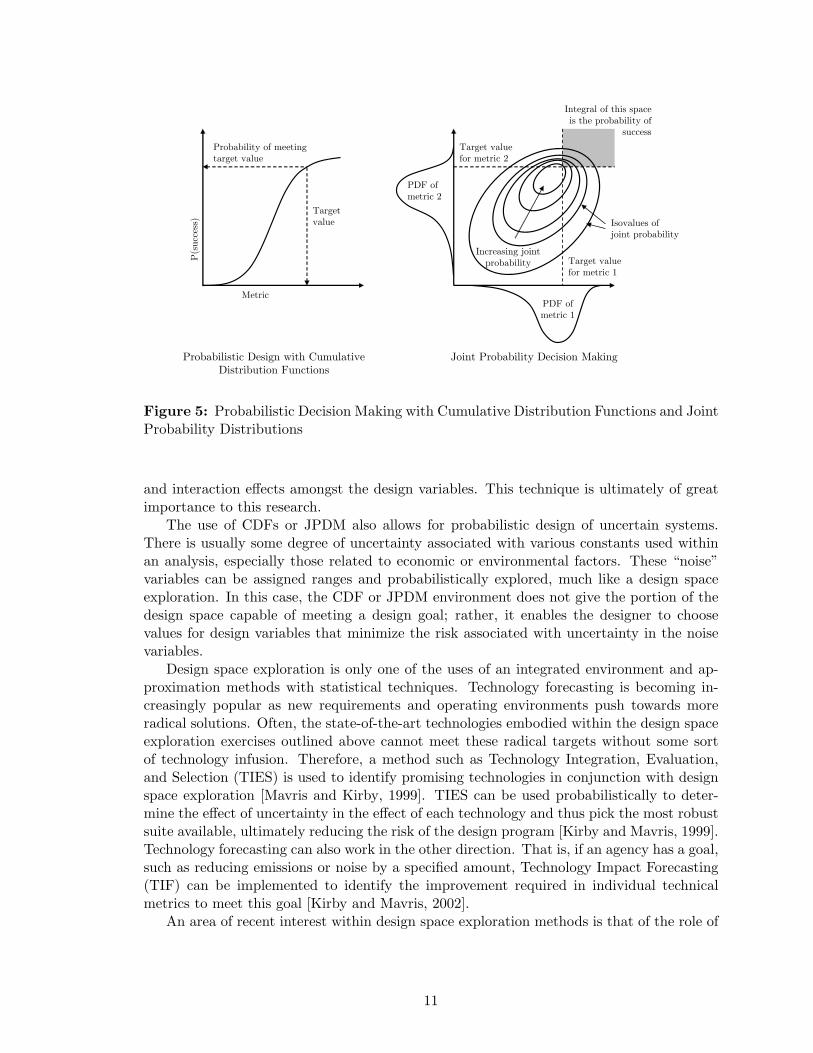
One drawback of working directly with the integrated environment is that the overallsystem evaluation time may be relatively long due to the execution times of the individualanalyses, in series or parallel. Even modern MDO methods may not enable an engineer torapidly investigate the entire design space available to a given concept. Therefore, high-fidelity approximations and statistical techniques can be used to speed up system executiontime and explore every concept available within the design space. Three principle methodsare capable of this: Monte Carlo Simulation (MCS) of the design space combined with theoriginal integrated environment, MCS of the design space combined with a surrogate model(approximation) of the original environment, or Fast Probability Integration (FPI) of thedesign space combined with the original environment [Fox, 1994; Mavris and Bandte, 1997].The first is the highest fidelity solution but takes the most time; the latter two providetime savings at reductions in fidelity. All of these techniques rely on the generation ofCumulative Distribution Functions (CDFs) to determine the portion of the design spacethat can satisfy the specified requirements. These CDFs can be viewed individually todetermine the probability of success for a given metric. However, this does not determinethe probability of meeting more than just one particular metric. Bandte’s Joint ProbabilityDecision Making (JPDM) technique combines the Probability Density Functions (PDFs)generated during probabilistic design to determine the portion of the design space that canmeet more than one requirement [Bandte, 2000]. An illustration of a single CDF and ajoint distribution function is given in Figure 5.

Several studies have been made using MCS with polynomial approximations [Mavrisand Bandte, 1995; DeLaurentis et al., 1996], as well as MCS with FPI [Mavris et al., 1997].A popular method for approximation of relatively well-behaved systems is Response SurfaceMethodology (RSM) [Neter et al., 1996] because it is capable of capturing linear, non-linear,

10

P(suc

cess)

Metric

Target value

Probability of meeting target value

Probabilistic Design with Cumulative Distribution Functions

PDF of metric 2

PDF of metric 1

Isovalues of joint probability

Increasing joint probability Target value

for metric 1

Integral of this space is the probability of

successTarget value for metric 2

Joint Probability Decision Making

Figure 5: Probabilistic Decision Making with Cumulative Distribution Functions and JointProbability Distributions

and interaction effects amongst the design variables. This technique is ultimately of greatimportance to this research.

The use of CDFs or JPDM also allows for probabilistic design of uncertain systems.There is usually some degree of uncertainty associated with various constants used withinan analysis, especially those related to economic or environmental factors. These “noise”variables can be assigned ranges and probabilistically explored, much like a design spaceexploration. In this case, the CDF or JPDM environment does not give the portion of thedesign space capable of meeting a design goal; rather, it enables the designer to choosevalues for design variables that minimize the risk associated with uncertainty in the noisevariables.

Design space exploration is only one of the uses of an integrated environment and ap-proximation methods with statistical techniques. Technology forecasting is becoming in-creasingly popular as new requirements and operating environments push towards moreradical solutions. Often, the state-of-the-art technologies embodied within the design spaceexploration exercises outlined above cannot meet these radical targets without some sortof technology infusion. Therefore, a method such as Technology Integration, Evaluation,and Selection (TIES) is used to identify promising technologies in conjunction with designspace exploration [Mavris and Kirby, 1999]. TIES can be used probabilistically to deter-mine the effect of uncertainty in the effect of each technology and thus pick the most robustsuite available, ultimately reducing the risk of the design program [Kirby and Mavris, 1999].Technology forecasting can also work in the other direction. That is, if an agency has a goal,such as reducing emissions or noise by a specified amount, Technology Impact Forecasting(TIF) can be implemented to identify the improvement required in individual technicalmetrics to meet this goal [Kirby and Mavris, 2002].

An area of recent interest within design space exploration methods is that of the role of

11

requirements in systems design. Often, the methods outlined above refer to static require-ments. The same statistical techniques can be applied to systems with varying requirements,and have been demonstrated with some success in conjunction with technology integration[Mavris and DeLaurentis, 2000; Baker and Mavris, 2001; Baker, 2002]. The research con-ducted within this document extends the work in the field.

2.3.2 Evolving Techniques

Of final interest in modern sizing methods is the recent introduction of volume-based tech-niques. Before, the vehicle scaling laws considered were simply based on gross weight.Now, an increased emphasis is being placed on how the system scales volumetrically. Somepreliminary “volume-balance” methods have been proposed by Raymer [Raymer, 2001].Volume-based methods will continue to evolve as more radical, low fuel density concepts,such as hydrogen-powered low-emission vehicles, are considered [Guynn and Olson, 2002].

2.4 Multi-Mission Approaches

From its inception, sizing an aircraft required an enumeration of mission requirements.This “design mission” thus formed the basis of the fuel-required curve in the range (orendurance) related vehicle scaling laws. The design mission is met when the fuel requiredto propel the vehicle along the specified mission profile matches the fuel available withinthe vehicle. Over time, the design mission began to resemble less of what mission thevehicle would actually fly, but rather became a series of limiting conditions for what thevehicle could be expected to accomplish over a series of similar missions. As identified inthe previous chapter, aircraft are increasingly being tasked with a wider variety of missions.This can make specification of a design mission difficult. One can envision several ways ofincorporating disparate mission profiles into a single sizing mission, but each will likely fallunder one of two main headings: size to the most critical mission, or size to a compositemission.

Sizing to the most critical mission is perhaps the simplest of these techniques and mostsimilar to current practices. In this method, the designer first defines the necessary missionprofiles and associated mission-specific performance, payload, and cost constraints. Thevehicle is sized to each of these secondary missions subject to the various point-performanceconstraints associated to that particular mission, as well as the general non-mission specificconstraints. Ultimately, the mission resulting in the largest gross weight vehicle becomes theonly mission capable of meeting all of the other mission (fuel) requirements, and thereforebecomes the de facto design mission. In this way, the vehicle is “overdesigned” with respectto some mission performance (range and endurance) metrics, though often others will suffer,such as off-design performance on the secondary missions and program cost.

One way to eliminate the potential for overdesign is to build a composite mission profilecapable of parametrically modeling each of the specified missions. This composite missionwould contain variable-length segments where necessary. These variables form a “missionspace” that can be evaluated separately or together with the design space of the vehicle[Baker and Mavris, 2001]. Variation of both design and mission space values gives thedesigner a tool to further envision tradeoffs amongst the design variables and requirements.Ultimately, this can be quite helpful in choosing the final design mission when sizing thevehicle, and is the first step in eliminating the concept of a design mission entirely. Eachpoint within the mission space represents a unique design mission to which the vehicle is

12

sized. Secondary performance variables can be tracked and traded off in such a way that asolution may not meet the most stringent mission requirements, but may be able to moreaffordably meet most of them.

2.4.1 Shortfalls

By its vary nature, multi-mission systems design fits naturally into the realm of MultipleCriteria Decision Making (MCDM) techniques, including such aspects as the relative impor-tance of each mission. This frame of mind is largely ignored through sizing-based techniqueslisted above as they always boil down to specification of a single design mission meant toencompass all of the vehicle requirements. As system concepts become more radical andthe specific missions required of the vehicle become more diverse, the chance of meetingall mission requirements (as in the first multi-mission sizing method) becomes improbable.Furthermore, “sizing” generally implies a fuel balance, which requires iteration and con-vergence to solve correctly. In a composite mission approach, large diversity in individualmissions may entail composite mission parameter ranges that lead to numerical instability.

A final point worth mentioning is that neither of these techniques is fully adaptableto design with uncertain requirements. Certainly, the mission space model can captureuncertainty in mission-related elements, but other constraints, such as point-performanceand cost may pose problems. The constraint lines can be moved, but constrained optimiza-tion techniques are not necessarily the best suited for probabilistic constraint evaluation.Instead, an unconstrained or penalty-function approach may be more appropriate for cap-turing uncertainty in system-level requirements.

2.4.2 Requirements Fitting for Multi-Mission Design

One problem with any form of multi-mission “sizing” is that a fuel balance is always implied.In order for a fuel balance to have any meaning, a unique design mission must be specifiedthat may or may not accurately represent the overall mission expectations of the aircraft.As mentioned above, the fuel balance was originally created as a method to estimate grossweight for mostly single-mission aircraft based on statistical scaling laws. It is possible to runthis process in reverse; that is, specify a gross weight and other pertinent design parametersand attempt to find what sorts of mission profiles the vehicle can fly. This is especiallywell-suited for multi-mission vehicle design because it becomes a simple matter to trackpertinent individual mission performance parameters (such as segment range, endurance,and point performance). Instead of a fuel balance, a parametric sweep of gross weight andother design parameters can be made, and mission performance tracked in each case. Thebest multi-mission aircraft would then be the vehicle with the design parameters and grossweight that best “fit” the individual mission requirements.

This approach is attractive because it makes MCDM an integral part of the designprocess. Now it is possible to directly tradeoff mission performance metrics for all of theindividual missions as well as other, non-mission specific metrics. This approach also mimicsthe “true” behavior of the system since the designer is virtually creating and test-flying aseries of vehicles that make up a decision-making environment. Finally, it is well-suitedfor automation as most aircraft analysis codes work much better and faster without theiteration and convergence required for a fuel balance.

13

CHAPTER III

DESIGN AND DECISION MAKING

Almost every aspect of life involves some form of decision making, whether it is large choicesuch as what job to pursue or a small choice such as what type of shirt to wear. Largeor small, each decision has consequences that require us to forecast the effect of variousalternatives. Once the choice is made, it is a matter of time to find whether the forecastwas spot-on or far off due to some unexpected event.

Engineering design also involves decision making and forecasting, though the methodsused appear to be far more concrete, at least on the surface. However, when one digs downfurther, the number of assumptions within an analysis that is the basis of a design decisionmay be inaccurate. Thus, engineering design will have some degree of uncertainty.

Many design decisions involve the use of mathematical or numerical optimization toreach an “ideal” setting of variables with respect to a single criterion. Unfortunately,optimization is not a substitute for decision making. Zeleny [Zeleny, 1982] challenges hisreaders with the statement:

No decision making occurs unless at least two criteria are present. If only onecriterion exists, mere measurement and search suffice for making a choice.

This implies that single-objective optimization is not decision making at all. An analogyfor the existence of multiple criteria in decision making can be made in the choice of shirtto wear. One may consider comfort, appearance, setting, and many other criteria even inthis simple case. If only comfort were important than one would simply have to searchthrough their closet and find the most comfortable shirt. Thus, optimization is more aboutdeveloping and executing the right search algorithm for a single-objective problem whereasdecision making is concerned with making a choice from multiple objectives.

Another necessary condition for decision-making is the availability of at least two distinctalternatives. Obviously, choosing which shirt to wear is a moot point if an individual onlyowns one shirt or 100 identical shirts. Of course, if the option exists to not wear a shirt atall, then a decision can be made amongst differentiated alternatives.

Unfortunately, humans are poor at making rational, repeatable decisions despite the factthat they experience decision making on a daily basis. This is especially true when thereare many more than two criteria to consider. The subjective nature of decision making,along with inherent biases and lack of proper processing of information, can lead to poorjudgement. Shepard [Shepard, 1964] notes:

At the level of the perceptual analysis of raw sensory inputs, man evinces aremarkable ability to integrate the responses of a vast number of receptive ele-ments according to exceedingly complex nonlinear rules. Yet once the profusionand welter of this raw input has been thus reduced to a set of usefully invariantconceptual objects, properties, and attributes, there is little evidence that theycan in turn be juggled and recombined with anything like this facility.

Shepard continues in this work by referring to a two-dimensional experiment with lin-early correlated attributes. The subjects surveyed would make a plethora of choices related

14

to individual biases in one or the other dimensions. He concludes that while humans arecapable of making subjective decisions, one should have some sort of computational aid tothe process if at all possible.

Certainly, one needs some sort of analytical means to help evaluate and select conceptswith multiple attributes. What follows is a description of some important components anda few selected techniques in Multiple Criteria Decision Making (MCDM).

3.1 Pareto Optimality

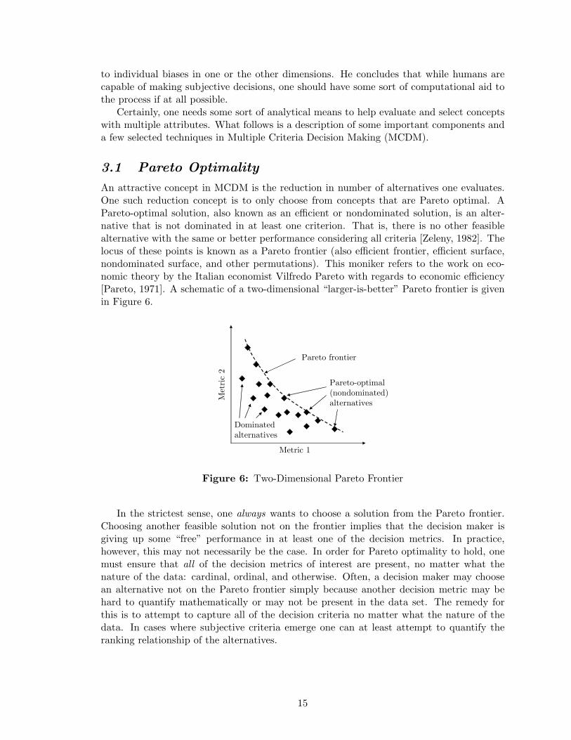
An attractive concept in MCDM is the reduction in number of alternatives one evaluates.One such reduction concept is to only choose from concepts that are Pareto optimal. APareto-optimal solution, also known as an efficient or nondominated solution, is an alter-native that is not dominated in at least one criterion. That is, there is no other feasiblealternative with the same or better performance considering all criteria [Zeleny, 1982]. Thelocus of these points is known as a Pareto frontier (also efficient frontier, efficient surface,nondominated surface, and other permutations). This moniker refers to the work on eco-nomic theory by the Italian economist Vilfredo Pareto with regards to economic efficiency[Pareto, 1971]. A schematic of a two-dimensional “larger-is-better” Pareto frontier is givenin Figure 6.

Metric 1

Met

ric 2

Pareto frontier

Dominated alternatives

Pareto-optimal (nondominated) alternatives

Figure 6: Two-Dimensional Pareto Frontier

In the strictest sense, one always wants to choose a solution from the Pareto frontier.Choosing another feasible solution not on the frontier implies that the decision maker isgiving up some “free” performance in at least one of the decision metrics. In practice,however, this may not necessarily be the case. In order for Pareto optimality to hold, onemust ensure that all of the decision metrics of interest are present, no matter what thenature of the data: cardinal, ordinal, and otherwise. Often, a decision maker may choosean alternative not on the Pareto frontier simply because another decision metric may behard to quantify mathematically or may not be present in the data set. The remedy forthis is to attempt to capture all of the decision criteria no matter what the nature of thedata. In cases where subjective criteria emerge one can at least attempt to quantify theranking relationship of the alternatives.

15

3.2 Axiomatic Design

While not explicitly under the heading of MCDM, Axiomatic Design is a process that seeksto resolve some of the issues with designing to multiple requirements. Notably, it attemptsto remove conflict by maintaining independence amongst requirements. Suh defines twodesign axioms [Suh, 1990] as:

The Independence Axiom: Maintain the independence of the Functional Re-quirements (FRs).

The Information Axiom: Minimize the information content of the design.

The independence axiom ultimately establishes that the Functional Requirements mustbe independent such that only one is modified for any perturbation of a Design Parameter(DP). The information axiom states that the best design is the one which minimizes thenumber of FRs and DPs required to define the design.

An oft-used axiomatic design example is the choice of water faucet for household use asseen in Figure 7. In this case, the FRs are to control water temperature and water flow rate.A typical, “bad” design for a faucet has two handles and one spigot; one handle controlsthe flow of hot water and one of cold water. Here, one cannot independently control eithertemperature or flow rate; rather, the user must modify inputs to both handles to change oneof the outputs. The Axiomatic Design approach would select a more modern faucet with atwo-degree of freedom handle. In the latter case, the vertical rotation of the handle controlsthe flow rate and the horizontal rotation controls the temperature. Here, the independenceof the FRs is maintained with respect to the DPs.

Standard design Axiomatic design

Figure 7: Axiomatic Faucet Design [MIT Axiomatic Design Group, 2005]

In theory, Axiomatic Design seems to be a good approach for design. In practice it maybe much harder to enforce, especially in systems engineering situations where the designparameters are high-level abstractions of individual systems and the functional requirementsare industry or government standards. Often it becomes impossible or improbable to discernindividual inputs for the design parameters. An aggregate set of requirements may bepossible but difficult to relate. If a decomposition-based approach were used, it may becomepossible to create a set of independent functional requirements with transparency to theoriginal requirements, though it would be much harder to enforce independence of designparameters. The attractive feature of independent requirements lies in the decision-makingitself: if the requirements are truly independent there should be no bias from one solutionto the next.

16

3.3 Multiple Criteria Decision Making Techniques

Multiple Criteria Decision Making is a necessarily broad subject area. There are manyclasses and subgroups of methods depending on the nature of the criteria considered, theinvolvement of the decision maker, and the nature of the objective sought. Though theopinions of many authors differ on the subject, in this document MCDM will be usedto refer to two different classes of methods: Multiple Attribute Decision Making (MADM)and Multiple Objective Decision Making (MODM) [Yoon and Hwang, 1995]. Some considerMultiple Attribute Utility Theory (MAUT) to be under this heading as well, but this subjectwill not be covered in detail here.

The principle difference between MADM and MODM techniques is the pertinent ap-plication. MADM techniques are focused on ranking and selection of a few options froma discrete pool of alternatives, usually not subject to constraints [Hwang and Yoon, 1981].On the surface, MADM is more appropriate when a decision maker must choose from apool of predefined concepts, such as the government’s choice of five competing fighter con-figurations from different companies or one’s choice of a stock portfolio. MODM techniquesare more appropriate for design applications, as they focus on multiple objectives withina continuous space and are subject to active constraints [Hwang and Masud, 1979]. Bothtechniques capitalize on various weighting techniques to determine ranking or preferencerelationships between the various criteria.

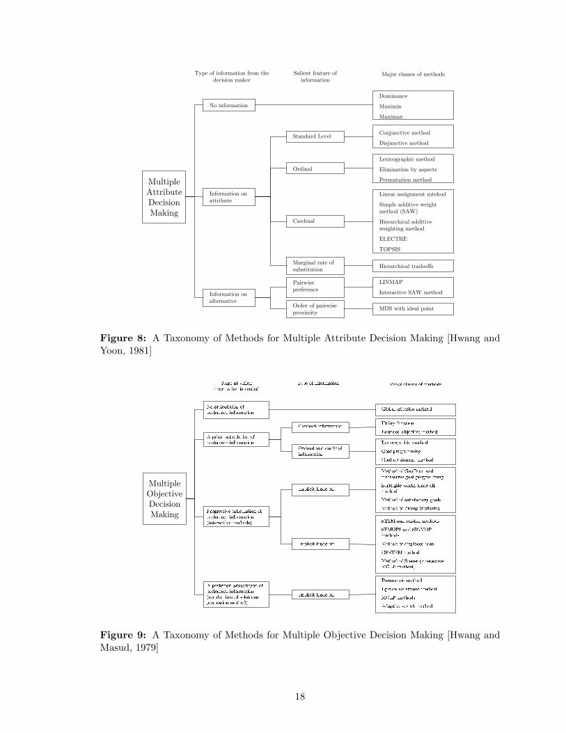
A variety of techniques are available for both MADM and MODM depending on thenature of the information available to the decision maker or algorithm. Figures 8 and 9are reproduced from the work of Hwang and his colleagues [Hwang and Yoon, 1981; Hwangand Masud, 1979] and display a taxonomy of MADM and MODM techniques, respectively.Note that MADM techniques vary by the type of information available whereas MODMtechniques are categorized by both the type of information and the stage at which thisinformation is needed.

The decisions made within aerospace systems design usually refer to cardinal data;that is, data associated with a quantity but not necessarily a preferential order (note that aranking relationship may be derived from cardinal data if a goal or direction of improvementis noted). The data retrieved from engineering analyses are, with few exceptions, cardinal.Examples include gross weight, cost, sustained turn rate, and takeoff field length, to namea few. Some more subjective criteria may be ordinal in nature, that is, simply ranked withrespect to the other alternatives. An example may be a qualitative measure of reliabilityas low, medium, or high. This is far less common in engineering analysis. Therefore, onlysome of the cardinal methods shown in Figures 8 and 9 or their associated outgrowths willbe elaborated upon further. For a more complete description of these techniques the readeris directed to more comprehensive references [Hwang and Masud, 1979; Hwang and Yoon,1981; Zeleny, 1982; Triantaphyllou, 2000].

3.3.1 The Ideal Solution

A powerful concept in cardinal MCDM techniques is that of the ideal solution. This is thesolution that embodies the best answer within the design domain for each of the attributes.Mathematically, the ideal solution can be stated as

Y ∗ = (y∗1, y∗2, . . . , y∗n) (1)

where Y ∗ is the ideal solution and y∗n is the best value of the nth attribute. This solutionis often made up of attributes from multiple alternatives (if such a solution was available

17

Multiple Attribute Decision Making

No information

Information on attribute

Information on alternative

Type of information from the decision maker

Salient feature of information Major classes of methods

Standard Level

Ordinal

Cardinal

Marginal rate of substitutionPairwisepreference

Order of pairwiseproximity

DominanceMaximinMaximax

Conjunctive methodDisjunctive method

Lexicographic methodElimination by aspectsPermutation methodLinear assignment mtehodSimple additive weight method (SAW)Hierarchical additive weighting methodELECTRETOPSIS

Hierarchical tradeoffs

MDS with ideal point

LINMAPInteractive SAW method

Figure 8: A Taxonomy of Methods for Multiple Attribute Decision Making [Hwang andYoon, 1981]

Multiple Objective Decision Making

��

��

��

��

��

��

��

� ��

� ��

��!��

"��#��!��$� ��%��

�� $�� &��'��

�� ()�� () �� )��

��$��(%) ��

)�� (%) ��$��

)��$�� $� ��

(��

Figure 9: A Taxonomy of Methods for Multiple Objective Decision Making [Hwang andMasud, 1979]

18

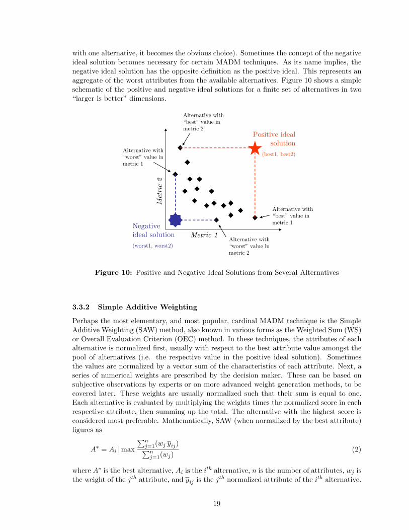
with one alternative, it becomes the obvious choice). Sometimes the concept of the negativeideal solution becomes necessary for certain MADM techniques. As its name implies, thenegative ideal solution has the opposite definition as the positive ideal. This represents anaggregate of the worst attributes from the available alternatives. Figure 10 shows a simpleschematic of the positive and negative ideal solutions for a finite set of alternatives in two“larger is better” dimensions.

Metric 1

Met

ric

2

Positive ideal solution

(best1, best2)

Negative ideal solution(worst1, worst2)

Alternative with “best” value in metric 1

Alternative with “best” value in metric 2

Alternative with “worst” value in metric 2

Alternative with “worst” value in metric 1

Figure 10: Positive and Negative Ideal Solutions from Several Alternatives

3.3.2 Simple Additive Weighting

Perhaps the most elementary, and most popular, cardinal MADM technique is the SimpleAdditive Weighting (SAW) method, also known in various forms as the Weighted Sum (WS)or Overall Evaluation Criterion (OEC) method. In these techniques, the attributes of eachalternative is normalized first, usually with respect to the best attribute value amongst thepool of alternatives (i.e. the respective value in the positive ideal solution). Sometimesthe values are normalized by a vector sum of the characteristics of each attribute. Next, aseries of numerical weights are prescribed by the decision maker. These can be based onsubjective observations by experts or on more advanced weight generation methods, to becovered later. These weights are usually normalized such that their sum is equal to one.Each alternative is evaluated by multiplying the weights times the normalized score in eachrespective attribute, then summing up the total. The alternative with the highest score isconsidered most preferable. Mathematically, SAW (when normalized by the best attribute)figures as

A∗ = Ai |max

∑nj=1(wj yij)∑n

j=1(wj)(2)

where A∗ is the best alternative, Ai is the ith alternative, n is the number of attributes, wj isthe weight of the jth attribute, and yij is the jth normalized attribute of the ith alternative.

19

If “larger is better” for all yj , then the normalization follows as

yij =yij

y∗j(3)

where yij is the “raw” value of the jth attribute of the ith alternative. For a “smaller isbetter” case, the reciprocal of (3) is used.

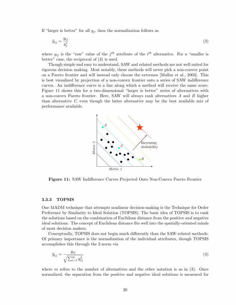
Though simple and easy to understand, SAW and related methods are not well suited forrigorous decision making. Most notably, these methods will never pick a non-convex pointon a Pareto frontier and will instead only choose the extremes [Mullur et al., 2003]. Thisis best visualized by projection of a non-convex frontier onto a series of SAW indifferencecurves. An indifference curve is a line along which a method will receive the same score.Figure 11 shows this for a two-dimensional “larger is better” series of alternatives witha non-convex Pareto frontier. Here, SAW will always rank alternatives A and B higherthan alternative C, even though the latter alternative may be the best available mix ofperformance available.

Met

ric

2

Metric 1

A

B

CIncreasing desirability

Figure 11: SAW Indifference Curves Projected Onto Non-Convex Pareto Frontier

3.3.3 TOPSIS

One MADM technique that attempts nonlinear decision-making is the Technique for OrderPreference by Similarity to Ideal Solution (TOPSIS). The basic idea of TOPSIS is to rankthe solutions based on the combination of Euclidean distance from the positive and negativeideal solutions. The concept of Euclidean distance fits well into the spatially-oriented mindsof most decision makers.

Conceptually, TOPSIS does not begin much differently than the SAW-related methods.Of primary importance is the normalization of the individual attributes, though TOPSISaccomplishes this through the 2-norm via

yij =yij√∑mi=1 y2

ij

(4)

where m refers to the number of alternatives and the other notation is as in (3). Oncenormalized, the separation from the positive and negative ideal solutions is measured for

20

each alternative through

S∗i =

√√√√n∑

j=1

(wj(yij − y∗j )

)2 (5)

S−i =

√√√√n∑

j=1

(wj(yij − y−j )

)2 (6)

where Si refers to the separation measure, the subscript ‘∗’ refers to the positive idealsolution, and ‘−’ refers to the negative ideal solution. All other notation is as before.

These separation measures are combined into a single measure dubbed the closeness tothe ideal solution for each alternative. This is figured from

C∗i =

S−iS∗i + S−i

(7)

where C∗i is the closeness measure for the ith alternative. The solutions are then ranked in

descending order; i.e. the alternative with the highest value for C∗i is considered the “best,”

with the next-highest value as the “second-best,” and so on.The 2-norm would seem to indicate that this method is capable of capturing some non-

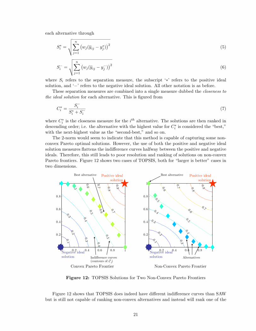
convex Pareto optimal solutions. However, the use of both the positive and negative idealsolution measures flattens the indifference curves halfway between the positive and negativeideals. Therefore, this still leads to poor resolution and ranking of solutions on non-convexPareto frontiers. Figure 12 shows two cases of TOPSIS, both for “larger is better” cases intwo dimensions.

0 0.2 0.4 0.6 0.8 10

0.2

0.4

0.6

0.8

10 .1

0.2

0.3

0.3

0 .4

0.4

0. 5

0. 5

0. 5

0 .6

0.60. 7

0.70. 8

0.9

0 0.2 0.4 0.6 0.8 10

0.2

0.4

0.6

0.8

1

0.10.2

0 . 3

0. 3

0.4

0 .4

0.5

0.5

0. 6

0.6

0 .7

0.7

0. 8

0. 9


Negative ideal solution


Negative ideal solutionIndifference curves

(contours of C*�)Alternatives

Best alternative Best alternative

Convex Pareto Frontier Non-Convex Pareto Frontier

Figure 12: TOPSIS Solutions for Two Non-Convex Pareto Frontiers

Figure 12 shows that TOPSIS does indeed have different indifference curves than SAWbut is still not capable of ranking non-convex alternatives and instead will rank one of the

21

extreme alternatives in this situation. The behavior of TOPSIS indifference curves is citedby Yoon [Yoon and Hwang, 1995] as being rational. He states:

When a [decision maker] recognize’s ones solution is closer to the negative-idealthan to the positive-ideal, the [decision maker] is inclined to pick an alternativethat consists of the best and worst attributes rather than one with two worseattributes. For example, one might want to get one A grade and one F graderather than two D grades.

This choice reflects one of the caveats of TOPSIS: the assumption of monotonicallyincreasing utility. Unfortunately, this may not always be a valid assumption. Therefore,methods that are able to capture some shallow non-convex solutions may be more appro-priate when a decision maker is willing to enable larger tradeoffs to achieve a compromise.

3.3.4 Compromise Programming

Compromise Programming (CP) is a quasi-MODM technique that is a combination of Multi-objective Linear Programming and Goal Programming [Zeleny, 1982]. The former approachis an extension of the popular linear programming techniques, such as the Simplex method[Chvatal, 1983] for problems with multiple objectives, hence its MODM identification. Goalprogramming is usually a linear programming technique as well, except with modified ob-jective functions to reflect a specific goal. This is more of a “nominal the best” style ofoptimization where the goals frequently lie within the design domain but may not neces-sarily be a maximum or minimum of the alternatives within the concept space (hence thequasi-MODM identification). Compromise programming is very flexible and can be usedfor nonlinear problems. It too uses the concept of the positive ideal solution and in somecases the negative ideal solution, sometimes referred to in the literature as the “anti-ideal.”

A popular method for CP uses the positive and negative ideal solutions (or, in a con-tinuous space, the “best” and “worst” values) and has an objective function of the form[Zeleny, 1982; Vanderplaats, 1999]

F (~x) =

{n∑

j=1

[wj(Fj(~x)− F ∗

j )

F−j − F ∗

j

]p} 1

p

(8)

where F (~x) is the overall objective function to be minimized, ~x is a vector of the designvariables, Fj(~x) is the jth objective (attribute) function, F ∗

j is the “best” value of Fj(~x)(analogous to y∗j in (3)), F−

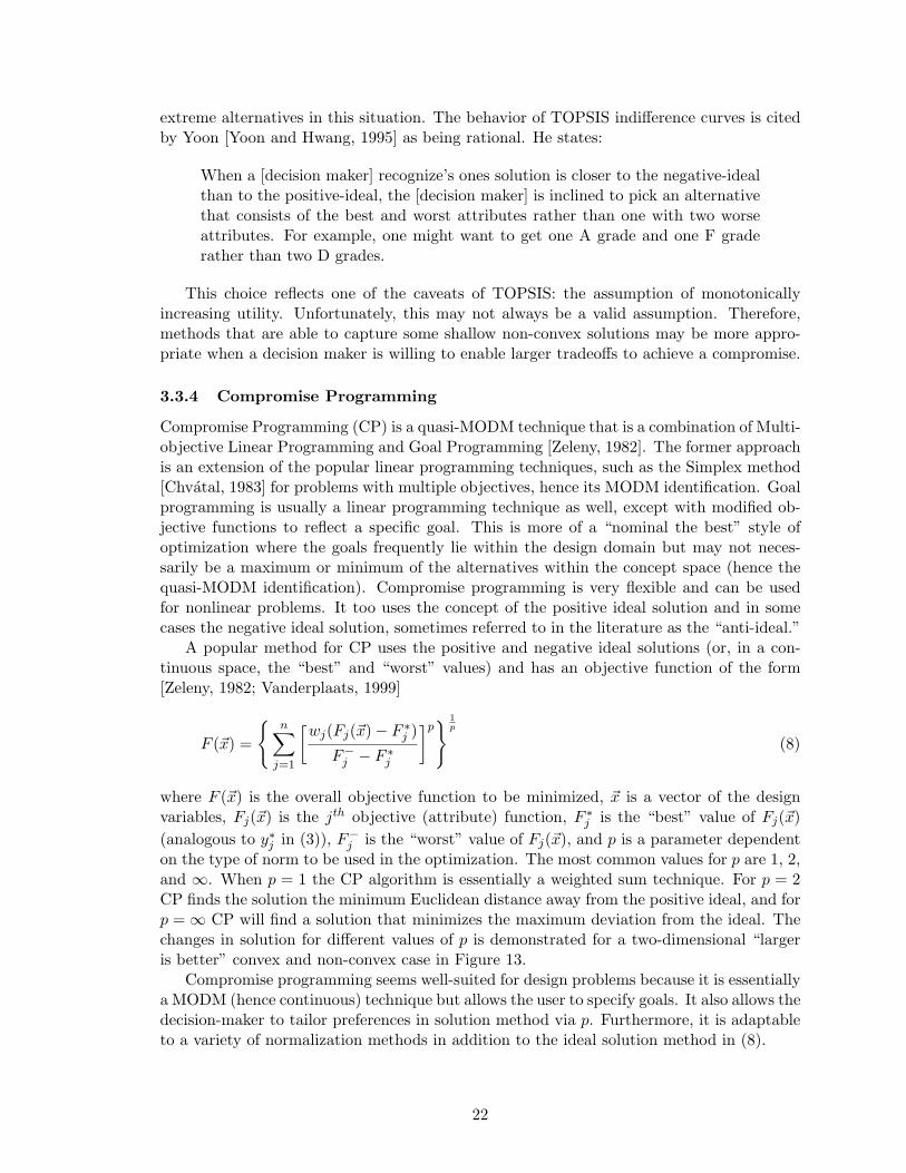
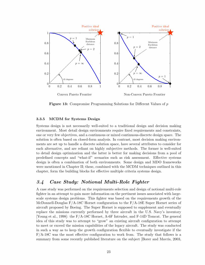
j is the “worst” value of Fj(~x), and p is a parameter dependenton the type of norm to be used in the optimization. The most common values for p are 1, 2,and ∞. When p = 1 the CP algorithm is essentially a weighted sum technique. For p = 2CP finds the solution the minimum Euclidean distance away from the positive ideal, and forp = ∞ CP will find a solution that minimizes the maximum deviation from the ideal. Thechanges in solution for different values of p is demonstrated for a two-dimensional “largeris better” convex and non-convex case in Figure 13.

Compromise programming seems well-suited for design problems because it is essentiallya MODM (hence continuous) technique but allows the user to specify goals. It also allows thedecision-maker to tailor preferences in solution method via p. Furthermore, it is adaptableto a variety of normalization methods in addition to the ideal solution method in (8).

22

0 0.2 0.4 0.6 0.8 10

0.2

0.4

0.6

0.8

1

0 0.2 0.4 0.6 0.8 10

0.2

0.4

0.6

0.8

1

Convex Pareto Frontier Non-Convex Pareto Frontier



45 degrees 45 degrees

Minimum Euclidean distance Minimum

Euclidean distance

p = 1

p = 2

p = ∞

p = ∞

p = 1

p = 1

p = 2

Figure 13: Compromise Programming Solutions for Different Values of p

3.3.5 MCDM for Systems Design

Systems design is not necessarily well-suited to a traditional design and decision makingenvironment. Most detail design environments require fixed requirements and constraints,one or very few objectives, and a continuous or mixed continuous-discrete design space. Thesolution is often based on closed-form analysis. In contrast, most decision making environ-ments are set up to handle a discrete solution space, have several attributes to consider foreach alternative, and are reliant on highly subjective methods. The former is well-suitedto detail design optimization and the latter is better for making decisions from a pool ofpredefined concepts and “what-if” scenarios such as risk assessment. Effective systemsdesign is often a combination of both environments. Some design and MDO frameworkswere mentioned in Chapter II; these, combined with the MCDM techniques outlined in thischapter, form the building blocks for effective multiple criteria systems design.

3.4 Case Study: Notional Multi-Role Fighter

A case study was performed on the requirements selection and design of notional multi-rolefighter in an attempt to gain more information on the pertinent issues associated with large-scale systems design problems. This fighter was based on the requirements growth of theMcDonnell-Douglas F/A-18C Hornet configuration to the F/A-18E Super Hornet series ofaircraft proposed by Boeing. The Super Hornet is supposed to supplement and eventuallyreplace the missions currently performed by three aircraft in the U.S. Navy’s inventory[Young et al., 1998]: the F/A-18C Hornet, A-6F Intruder, and F-14D Tomcat. The generalidea of this study was to attempt to “grow” an existing aircraft configuration to attemptto meet or exceed the mission capabilities of the legacy aircraft. The study was conductedin such a way as to keep the growth configuration flexible to eventually investigate if theF/A-18C was the most effective configuration to work from. The study that follows is asummary from some recently published literature on the subject [Borer and Mavris, 2003,

23

2004]. The reader is referred to these documents for a more comprehensive review.

3.4.1 Problem Formulation

The main formulation of this study involved six steps: Requirements Classification, Base-line Concept Definition, Creation of Integrated Environment, Decision Space Population,Exploration of Requirements Tradeoffs, and finally, Decision Making. The first step wasuniversal for all configurations, while steps two through five could be repeated for differentconcepts if necessary. The final decision could be based on the results from several con-cepts. This study only considered the F/A-18C configuration but the overall formulationwas generic enough that any (or several) baselines could be used.

The requirements classification followed from examination of the missions of the legacyaircraft the Super Hornet was meant to replace. However, some of the latest data onthe legacy aircraft was not available, so data was used from earlier models of the sameaircraft. The mission requirements and profiles were collated from the Standard AircraftCharacteristics (SAC) charts of the F/A-18C [Naval Air Systems Command, 1996], A-6E[Naval Air Systems Command, 1984], and F-14A [Naval Air Systems Command, 1976]. Intotal, these aircraft performed 21 missions, though there was redundant capability amongstthe legacy aircraft so they only accounted for nine distinct mission profiles (albeit withdifferent individual capabilities). For the most part, the most critical (in terms of payload-range) mission parameters were chosen when multiple airframes flew the same missionprofile. These missions are depicted in Table 1 with the “dominant” configuration in bold.

Table 1: Notional Multi-Role Fighter Missions

Mission AircraftF/A-18CF-14AA-6E

F/A-18CF-14AA-6E

F/A-18CA-6E

F/A-18CF-14AA-6E

Lo-Lo-Hi F-14AF/A-18CF-14AA-6E

F/A-18CF-14A

F/A-18CF-14A

F/A-18CF-14A

Close Support

Fighter Escort

Deck-Launched Intercept

Combat Air Patrol

Hi-Hi-Hi

Lo-Lo-Lo

Hi-Lo-Hi

Hi-Lo-Lo-Hi / Interdiction

24

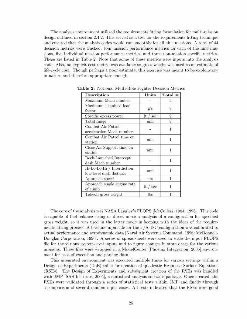
The analysis environment utilized the requirements fitting formulation for multi-missiondesign outlined in section 2.4.2. This served as a test for the requirements fitting techniqueand ensured that the analysis codes would run smoothly for all nine missions. A total of 44decision metrics were tracked: four mission performance metrics for each of the nine mis-sions, five individual mission performance metrics, and three non-mission specific metrics.These are listed in Table 2. Note that some of these metrics were inputs into the analysiscode. Also, no explicit cost metric was available so gross weight was used as an estimate oflife-cycle cost. Though perhaps a poor estimate, this exercise was meant to be exploratoryin nature and therefore appropriate enough.

Table 2: Notional Multi-Role Fighter Decision MetricsDescription Units Total #Maximum Mach number - 9Maximum sustained load factor g's 9Specific excess power ft / sec 9Total range nmi 9Combat Air Patrol acceleration Mach number - 1Combat Air Patrol time on station min 1Close Air Support time on station min 1Deck-Launched Intercept dash Mach number - 1Hi-Lo-Lo-Hi / Interdiction low-level dash distance nmi 1Approach speed kts 1Approach single engine rate of climb ft / sec 1Takeoff gross weight lbs 1

The core of the analysis was NASA Langley’s FLOPS [McCullers, 1984, 1998]. This codeis capable of fuel-balance sizing or direct mission analysis of a configuration for specifiedgross weight, so it was used in the latter mode in keeping with the ideas of the require-ments fitting process. A baseline input file for the F/A-18C configuration was calibrated toactual performance and aerodynamic data [Naval Air Systems Command, 1996; McDonnell-Douglas Corporation, 1996]. A series of spreadsheets were used to scale the input FLOPSfile for the various system-level inputs and to figure changes in store drags for the variousmissions. These files were wrapped in a ModelCenter [Phoenix Integration, 2005] environ-ment for ease of execution and parsing data.

This integrated environment was executed multiple times for various settings within aDesign of Experiments (DoE) table for creation of quadratic Response Surface Equations(RSEs). The Design of Experiments and subsequent creation of the RSEs was handledwith JMP [SAS Institute, 2005], a statistical analysis software package. Once created, theRSEs were validated through a series of statistical tests within JMP and finally througha comparison of several random input cases. All tests indicated that the RSEs were good

25

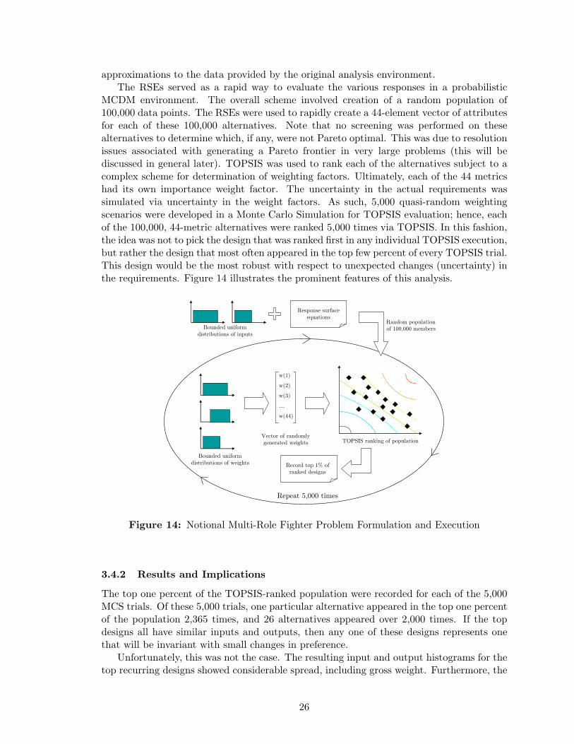
approximations to the data provided by the original analysis environment.The RSEs served as a rapid way to evaluate the various responses in a probabilistic

MCDM environment. The overall scheme involved creation of a random population of100,000 data points. The RSEs were used to rapidly create a 44-element vector of attributesfor each of these 100,000 alternatives. Note that no screening was performed on thesealternatives to determine which, if any, were not Pareto optimal. This was due to resolutionissues associated with generating a Pareto frontier in very large problems (this will bediscussed in general later). TOPSIS was used to rank each of the alternatives subject to acomplex scheme for determination of weighting factors. Ultimately, each of the 44 metricshad its own importance weight factor. The uncertainty in the actual requirements wassimulated via uncertainty in the weight factors. As such, 5,000 quasi-random weightingscenarios were developed in a Monte Carlo Simulation for TOPSIS evaluation; hence, eachof the 100,000, 44-metric alternatives were ranked 5,000 times via TOPSIS. In this fashion,the idea was not to pick the design that was ranked first in any individual TOPSIS execution,but rather the design that most often appeared in the top few percent of every TOPSIS trial.This design would be the most robust with respect to unexpected changes (uncertainty) inthe requirements. Figure 14 illustrates the prominent features of this analysis.

w(1)w(2)w(3)…

w(44)

Random population of 100,000 members

Bounded uniform distributions of weights

Vector of randomly generated weights TOPSIS ranking of population

Record top 1% of ranked designs

Repeat 5,000 times

Bounded uniform distributions of inputs

Response surface equations

Figure 14: Notional Multi-Role Fighter Problem Formulation and Execution

3.4.2 Results and Implications

The top one percent of the TOPSIS-ranked population were recorded for each of the 5,000MCS trials. Of these 5,000 trials, one particular alternative appeared in the top one percentof the population 2,365 times, and 26 alternatives appeared over 2,000 times. If the topdesigns all have similar inputs and outputs, then any one of these designs represents onethat will be invariant with small changes in preference.

Unfortunately, this was not the case. The resulting input and output histograms for thetop recurring designs showed considerable spread, including gross weight. Furthermore, the

26

recurrence was much smaller than hoped. At best, the top recurring design was in the topone percent 2,365 out of 5,000 trials, slightly more than 47% of the time. This level of riskis likely unacceptable for most programs. This could perhaps be increased with a smallerrange and refined distributions within the MCS trials, but seemed to be indicative of biggerproblems.

One such problem with this formulation was the incredible number of requirements.Unfortunately many of the requirements were highly dependent on the same parameters asothers, potentially creating “double-weighting” (and more) situations within the TOPSIStrial. That is, if two requirements were essentially the same metric, then including them inany MCDM approach will act as if that one metric were twice as important.

One final problem with any MCDM formulation is a lack of threshold values. Often,there is a threshold beyond which a decision maker becomes indifferent to the value of aparticular metric. TOPSIS and other MCDM formulations will essentially try to exploit theresponses with the greatest slope in finding a solution (this slope may be partially mitigatedwith the weighting factors). However, this may not be desirable once a metric reaches orapproaches a certain value, and instead the optimization effort should be spent in otherdimensions even if they have a lower slope.

3.4.3 Research Directions

In all, the notional multi-role fighter case study was a success. Though the results themselveswere inconclusive, the exercise demonstrated some of the issues associated with bringingMCDM to large-scale systems design problems.

Systems design involves decisions made early on in a process considering such thingsas risk, performance, and cost. As mentioned before, aircraft design is often fraught withuncertainty, especially with respect to requirements and constraints. As such, an effectivemultiple criteria systems design environment would be one that could handle uncertaintyin requirements specification. It would also need to be capable of identifying key tradeoffsand the requirements which drive these tradeoffs.

As a systems design problem grows to encompass more requirements, the complexityassociated with its MCDM environment grows. More solutions become Pareto optimal, andthe addition of uncertainty further muddies the water when attempting to find the bestcompromise solution.

Four principal questions arise from the observations made thus far. These have to dowith the idiosyncracies associated with probabilistic design and MCDM for many require-ments. These research questions are identified as follows:

(R1) Is there a design formulation that is better suited to integration of proba-bilistic MCDM techniques?

(R2) What is the best solution to MCDM with uncertain requirements?

(R3) What are the key tradeoffs amongst a large set of requirements?

(R4) Is it possible to identify an ideal tradeoff?

The reader is asked to keep these questions in mind as the research plan unfolds through-out the rest of this document. The first two questions relate to some of the probabilisticdesign methods already identified, but the latter two invite a new formulation for MCDMto help determine relative importance of metrics and the selection of tradeoff values.

27

CHAPTER IV

DECISION MAKING FOR LARGE-SCALE PROBLEMS

The techniques described in Chapter III begin to give an appreciation for the choices avail-able when choosing a formulation for design and decision making. The MCDM methodsespecially have a unique taxonomy depending on the nature of the decision data: discrete,continuous, ordinal, cardinal, and more. Unfortunately, all decision making methods havesome prominent drawbacks, especially with respect to large-scale problems. Some of theseissues were discussed in the notional multi-role fighter case study presented in the previouschapter. The most notable drawbacks are the assumption of monotonically increasing utilityfor each metric and also the dependence of the decision metrics on others. However, theseissues are not insurmountable and can be dealt with within the appropriate framework.What follows is the development of a probabilistic MCDM model that is better suited tolarge-scale problems. This formulation is developed and demonstrated in parallel with anexample problem to further illustrate the principles at work.

4.1 Generalized Probabilistic MCDM Formulation

Fundamental to the description of a large-scale MCDM environment is the creation of ageneralized probabilistic MCDM formulation. This environment should be able to captureuncertainty in the requirements themselves or in the decision maker’s preference regardingone metric over another. Three salient characteristics of such a formulation are as follows:

• Probabilistic

• Lack of internal constraints;

• Implicit tradeoffs.

As with the notional multi-role fighter, the probabilistic portion of this formulation canbe handled through the relative weights in the MCDM environment. A probabilistic relativeweight is analogous to the decision maker’s uncertainty regarding the relative importanceof one metric to the next. It follows that the consistently higher-ranked solution is robust(relatively invariant) with respect to the decision metrics and therefore represents the bestprobabilistic solution.

Lack of internal constraints is very important in such a formulation because these canbias an integrated environment or cause bad fits to data if surrogate models are used (asis often necessary for probabilistic analyses; refer to Chapter II for more details). Theseinternal constraints may require iteration and convergence that are not transparent to thedesigner and therefore can cause problems when specifying other requirements. Further-more, many constraints may actually be requirements or decision metrics and therefore itis important to allow the decision maker external access to these values.

Finally, any non-trivial decision making formulation requires tradeoffs. For large prob-lems, the sheer number of tradeoffs is a combinatorial of the number of metrics, i.e.four requirements involves up to 3 + 2 + 1 = 6 tradeoffs, ten requirements can involve

28

9 + 8 + 7 + 6 + 5 + 4 + 3 + 2 + 1 = 45 tradeoffs, and so on. Therefore, it quickly becomesdifficult to handle explicit tradeoffs. These can be made implicit with many MCDM for-mulations simply through definition of a positive and negative ideal solutions along withrelative weights. Compromise programming is an attractive option because it can normal-ize the data to the positive and negative ideal solutions, is a continuous formulation, andallows the decision maker flexibility regarding the type of tradeoff to be made via the 1-, 2-,or ∞-norm. Compromise programming will also always capture a nondominated solution[Ismail-Yahaya and Messac, 2002].

The generalized probabilistic MCDM formulation can be formally summarized via thestatement of three hypotheses:

(H1) Effective Multiple Criteria Decision Making requires an open, internallyunconstrained integrated environment.

(H2) Requirements uncertainty can be captured through probabilistic relativeimportance weights of the individual metrics. It follows that the conceptthat is most robust with respect to change in the requirements is the conceptwhose ranking is most invariant with respect to changes in these weights.

(H3) Tradeoffs amongst multiple requirements can be implicitly handled througha decision-making algorithm capable of compromise. This compromise is bestcharacterized with respect to the positive and negative ideal solutions.

4.1.1 Generating Alternatives

All MCDM techniques require a dataset from which to make decisions. This dataset isgenerally discrete for MADM techniques and continuous in MODM, though this is not arule. It is possible to represent a continuous space with a collection of random discretepoints and just as possible to represent most discrete points with some form of continuousfunction if necessary. In this vein, “generating alternatives” need not necessarily mean thegeneration of discrete alternatives. Rather, it may just as likely refer to characterization ofthe overall continuous decision space for later MCDM evaluation.

Ideally, a decision maker wishes to choose from those solutions that are Pareto optimal.Choosing from this subgroup ensures that all tradeoffs, implicit or otherwise, would occuramongst nondominated alternatives. While an attractive option in theory, resolution ofthe Pareto frontier becomes difficult as the number of objectives increases. This has beendocumented for multiobjective problems where evolutionary algorithms are used to gleaninformation on the Pareto frontier [Deb, 2001]. Here, an initial population is necessary andan estimate can be made as to what fraction of the population size will be nondominated.Guidance for population size selection for up to 10 objectives can be found in Figure 15.

Furthermore, the computational effort required to resolve nondominated solutions in-creases nonlinearly as the population size increases. As can be inferred from Figure 15,even large populations contain mostly nondominated solutions. This seems to imply thatpre-screening dominated solutions is not worth the computational savings realized from areduction in number of decision alternatives for problems with many objectives. The anal-ogy of fraction of nondominated population size can be carried over to continuous decisionspaces. Here, the Pareto optimal solutions would be a continuous subset of the decisionspace. As the number of decision metrics (objectives) increases, the portion of the decisionspace that is completely dominated decreases until it is insignificant. This leads to the nexthypothesis regarding large-scale MCDM:

29

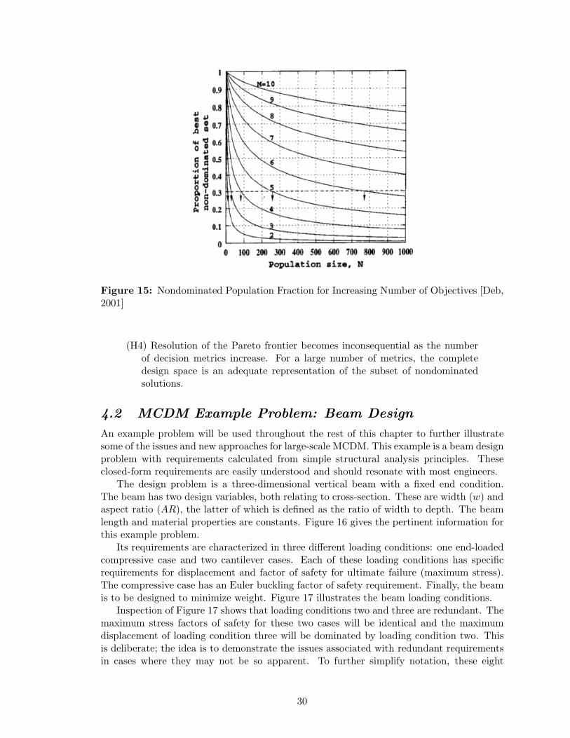
Figure 15: Nondominated Population Fraction for Increasing Number of Objectives [Deb,2001]

(H4) Resolution of the Pareto frontier becomes inconsequential as the numberof decision metrics increase. For a large number of metrics, the completedesign space is an adequate representation of the subset of nondominatedsolutions.

4.2 MCDM Example Problem: Beam Design

An example problem will be used throughout the rest of this chapter to further illustratesome of the issues and new approaches for large-scale MCDM. This example is a beam designproblem with requirements calculated from simple structural analysis principles. Theseclosed-form requirements are easily understood and should resonate with most engineers.

The design problem is a three-dimensional vertical beam with a fixed end condition.The beam has two design variables, both relating to cross-section. These are width (w) andaspect ratio (AR), the latter of which is defined as the ratio of width to depth. The beamlength and material properties are constants. Figure 16 gives the pertinent information forthis example problem.

Its requirements are characterized in three different loading conditions: one end-loadedcompressive case and two cantilever cases. Each of these loading conditions has specificrequirements for displacement and factor of safety for ultimate failure (maximum stress).The compressive case has an Euler buckling factor of safety requirement. Finally, the beamis to be designed to minimize weight. Figure 17 illustrates the beam loading conditions.

Inspection of Figure 17 shows that loading conditions two and three are redundant. Themaximum stress factors of safety for these two cases will be identical and the maximumdisplacement of loading condition three will be dominated by loading condition two. Thisis deliberate; the idea is to demonstrate the issues associated with redundant requirementsin cases where they may not be so apparent. To further simplify notation, these eight

30

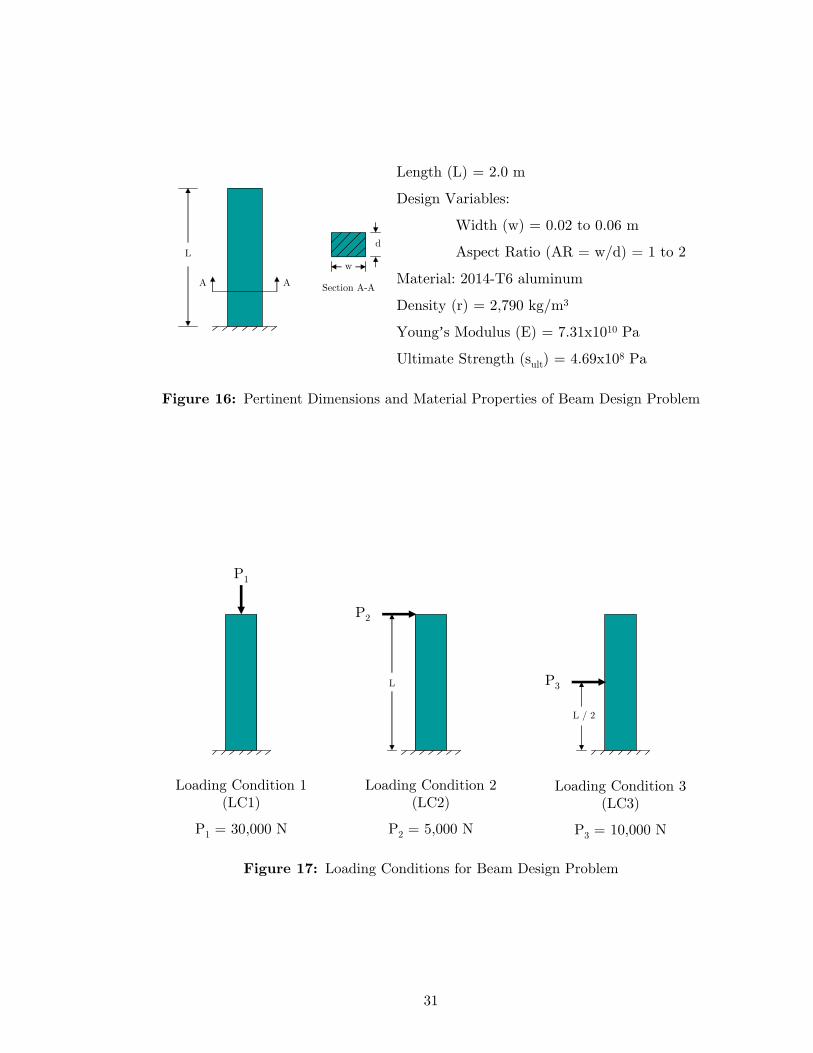
A A Section A-A

w

dL

Length (L) = 2.0 mDesign Variables:

Width (w) = 0.02 to 0.06 mAspect Ratio (AR = w/d) = 1 to 2

Material: 2014-T6 aluminumDensity (r) = 2,790 kg/m3

Young’s Modulus (E) = 7.31x1010 PaUltimate Strength (sult) = 4.69x108 Pa

Figure 16: Pertinent Dimensions and Material Properties of Beam Design Problem

P1

P2

P3

L / 2

L

Loading Condition 1 (LC1)

P1 = 30,000 N


P2 = 5,000 N


P3 = 10,000 N

Figure 17: Loading Conditions for Beam Design Problem

31

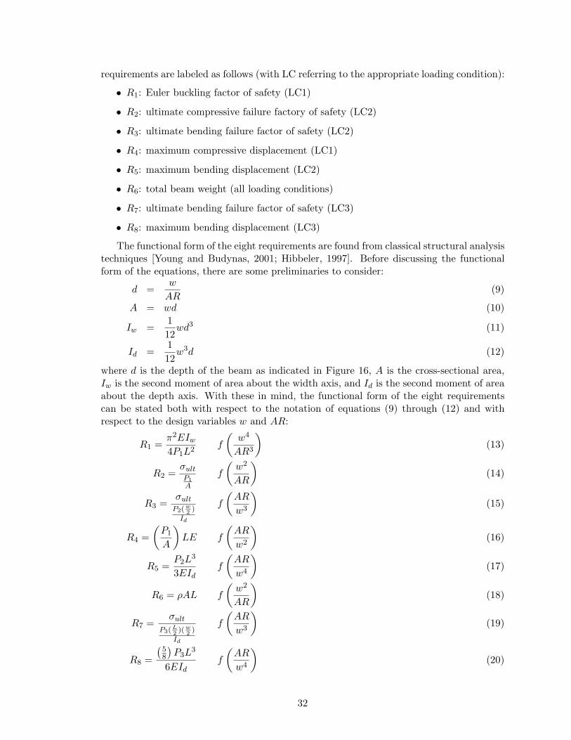
requirements are labeled as follows (with LC referring to the appropriate loading condition):

• R1: Euler buckling factor of safety (LC1)

• R2: ultimate compressive failure factory of safety (LC2)

• R3: ultimate bending failure factor of safety (LC2)

• R4: maximum compressive displacement (LC1)

• R5: maximum bending displacement (LC2)

• R6: total beam weight (all loading conditions)

• R7: ultimate bending failure factor of safety (LC3)

• R8: maximum bending displacement (LC3)

The functional form of the eight requirements are found from classical structural analysistechniques [Young and Budynas, 2001; Hibbeler, 1997]. Before discussing the functionalform of the equations, there are some preliminaries to consider:

d =w

AR(9)

A = wd (10)

Iw =112

wd3 (11)

Id =112

w3d (12)

where d is the depth of the beam as indicated in Figure 16, A is the cross-sectional area,Iw is the second moment of area about the width axis, and Id is the second moment of areaabout the depth axis. With these in mind, the functional form of the eight requirementscan be stated both with respect to the notation of equations (9) through (12) and withrespect to the design variables w and AR:

R1 =π2EIw

4P1L2f

(w4

AR3

)(13)

R2 =σultP1A

f

(w2

AR

)(14)

R3 =σult

P2(w2

)

Id

f

(AR

w3

)(15)

R4 =(

P1

A

)LE f

(AR

w2

)(16)

R5 =P2L

3

3EIdf

(AR

w4

)(17)

R6 = ρAL f

(w2

AR

)(18)

R7 =σult

P3(L2)(w

2)

Id

f

(AR

w3

)(19)

R8 =

(58

)P3L

3

6EIdf

(AR

w4

)(20)

32

where E refers to the Young’s modulus of elasticity, P1 through P3 is the load associatedwith loading conditions one through three, respectively, L refers to the beam length, and ρrefers to the material density.

Inspection of the functional forms given in equations (13) through (20) indicates thatonly five of these requirements are linearly independent. As expected, all of the LC3 re-quirements are the exact same functional form as the LC2 requirements; R7 will be perfectlycorrelated with R3, and R5 will be perfectly correlated with R8. Furthermore, two seem-ingly independent requirements, R2 and R6, are perfectly correlated. However, they areexactly opposite in terms of direction of improvement, but they will effectively cancel eachother out if the assumption of monotonically increasing utility is made. Also, the presenceof two functionally opposing objectives indicates that every solution within the design spaceis Pareto optimal since at least one of these two requirements will always be nondominated.

Basic engineering intuition leads to some assertions regarding this problem. First, therequirements of loading condition three should be completely dominated by loading con-dition two and therefore should not be a factor in the design problem (as long as theconstraints, if any, for LC3 are the same or lower than those for LC2). Further, the ap-parent “design drivers” appear to be Euler buckling and bending stress or displacement.Compressive failure factor of safety and compressive deflection should be minimal, andtherefore inconsequential to the final design.

4.2.1 Beam Analysis and Design Procedure

The MCDM formulation of the beam design problem emulates that of the notional multi-rolefighter as well as the general procedure outlined in section 4.1. The beam analysis code wasa series of files and functions created in Matlab [The Mathworks, Inc., 2005]. Though thisanalysis environment was very fast, this environment was used to create response surfaceequations of the eight requirements for a specified range of the design variables. The regionof interest was for a value of w from 0.05 to 0.10 meters and a value of AR from 1.0 to2.0. These values were varied within a five-level design of experiments to create third-order,fully interacting response surfaces for each requirement. Third-order response surfaces wereused because second-order surfaces could not provide a good approximation of the originalequations. These response surfaces are shown in Figure 18 for normalized inputs from -1.0to 1.0. The answers of the response surfaces were compared randomly to determine theirerror with respect to the original anlayses. The actual results are plotted versus the RSEresults in Figure 19.

Unless otherwise specified, the surrogate models of the requirements were used in allof the MCDM formulations. This ensured that the example problem would be executedsimilarly to a large-scale design problem (normally plagued with long execution times).These surrogate models form the objectives for the compromise programming algorithm,with the target values set at the positive ideal solution (always at the extreme of theequation). Each of the response surfaces are normalized by their mean and variance, so theycan never result in a value higher than 1.0 or lower than -1.0. They are also normalized suchthat all are “larger is better,” hence the deflection and weight equations are switched in sign.This is simply a matter of convention. The CP algorithm utilized the objective function fromequation (8) and minimized with a built-in Matlab function utilizing Sequential QuadraticProgramming (SQP) algorithm. SQP is a powerful gradient-based optimizer and is discussedat length in numerical optimization literature [Vanderplaats, 1999].

33

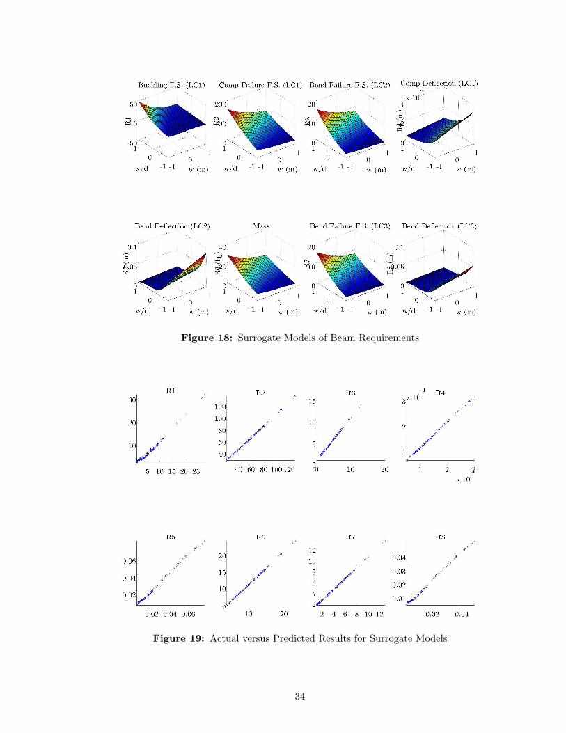
Figure 18: Surrogate Models of Beam Requirements

Figure 19: Actual versus Predicted Results for Surrogate Models

34

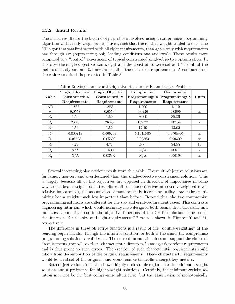
4.2.2 Initial Results

The initial results for the beam design problem involved using a compromise programmingalgorithm with evenly weighted objectives, such that the relative weights added to one. TheCP algorithm was first tested with all eight requirements, then again only with requirementsone through six (representing only loading conditions one and two). These results werecompared to a “control” experiment of typical constrained single-objective optimization. Inthis case the single objective was weight and the constraints were set at 1.5 for all of thefactors of safety and and 0.1 meters for all of the deflection requirements. A comparison ofthese three methods is presented in Table 3.

Table 3: Single and Multi-Objective Results for Beam Design Problem

ValueSingle Objective Constrained: 6 Requirements

Single Objective Constrained: 8 Requirements

Compromise Programming: 6 Requirements

Compromise Programming: 8 Requirements

Units

AR 1.865 1.865 1.000 1.119 -w 0.0558 0.0558 0.0920 0.0990 mR� 1.50 1.50 36.00 35.86 -R� 26.45 26.45 132.27 137.54 -R� 1.50 1.50 12.19 13.62 -R� 0.000249 0.000249 5.101E-05 4.670E-05 mR� 0.05603 0.05603 0.00583 0.00309 mR� 4.72 4.72 23.61 24.55 kgR� N/A 1.500 N/A 13.617 -R� N/A 0.03502 N/A 0.00193 m

Several interesting observations result from this table. The multi-objective solutions arefar larger, heavier, and overdesigned than the single-objective constrained solution. Thisis largely because all of the objectives are opposed in direction of importance in someway to the beam weight objective. Since all of these objectives are evenly weighted (evenrelative importance), the assumption of monotonically increasing utility now makes mini-mizing beam weight much less important than before. Beyond this, the two compromiseprogramming solutions are different for the six- and eight-requirement cases. This contrastsengineering intuition, which would normally have designed both beams the exact same andindicates a potential issue in the objective functions of the CP formulation. The objec-tive functions for the six- and eight-requirement CP cases is shown in Figures 20 and 21,respectively.

The difference in these objective functions is a result of the “double-weighting” of thebending requirements. Though the intuitive solution for both is the same, the compromiseprogramming solutions are different. The current formulation does not support the choice of“requirements groups” or other “characteristic directions” amongst dependent requirementsand is thus prone to such errors. The creation of such characteristic requirements couldfollow from decomposition of the original requirements. These characteristic requirementswould be a subset of the originals and would enable tradeoffs amongst key metrics.

Both objective functions also show a highly undesirable region near the minimum weightsolution and a preference for higher-weight solutions. Certainly, the minimum-weight so-lution may not be the best compromise alternative, but the assumption of monotonically

35

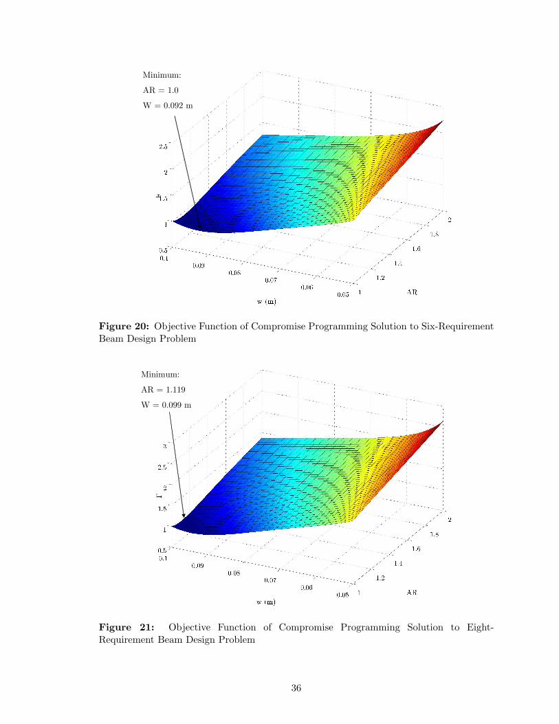
Minimum:AR = 1.0W = 0.092 m

Figure 20: Objective Function of Compromise Programming Solution to Six-RequirementBeam Design Problem

Minimum:AR = 1.119W = 0.099 m

Figure 21: Objective Function of Compromise Programming Solution to Eight-Requirement Beam Design Problem

36

increasing utility may not hold beyond a “threshold” value of the other requirements. Thecurrent formulation does not handle threshold or constraint values in the weighting scheme,instead having a static value for relative importance.

Two pertinent hypotheses can be formulated to better reflect the decision-makers pref-erence with respect to relative importance, threshold and constraint values, and the keytradeoffs in the decision process.

(H5) Dynamic relative importance weights better reflect the decision maker’spreference for constraints and threshold values.

(H6) Key tradeoffs can be identified and ranked through decomposition of theoriginal requirements. The best tradeoff is the solution closest to a theoretical“ideal tradeoff” in this subspace.

4.3 Weighting Schemes

The choice of the relative importance of each of the decision metrics is of paramount impor-tance to virtually every MCDM technique. As mentioned above, the relative importance ofeach metric should be dynamic to mimic the decision maker’s preference for constraints andthreshold values. Therefore, a two-part model for relative importance weights is suggested.This two-part model in its basic form is

wj = wsj + wd

j (~x) (21)

where wj is the relative importance (“weight”) of the jth metric, wsj is the static importance

of the metric, and wdj (~x) is the dynamic importance. The static importance is a reference

value given by the decision maker while the dynamic importance modifies the static valueto reflect the distance of the metric from the constraint and threshold values. Note that thedynamic value is a function of the design variables as it requires information on the currentvalue of the constraint. Uncertainty in the requirements can be captured with probabilitydistributions about the static weight.

Some requirements may be closely related to others. If requirements are “grouped” inany way, this would modify the overall relative importance given by equation (21). Require-ments grouping will be covered in a later section.

4.3.1 Entropy-Based Weights

The choice of static weights for individual metrics can follow from basic systems engineeringconcepts. These values are usually chosen by a qualified individual or panel of experts thatdebate the importance of one particular metric to another. However, it becomes increasinglydifficult to assign importance to individual requirements as their number and diversityincreases. Therefore, a decision maker needs some sort of aid when choosing static weights.

One promising concept is the idea of entropy-based weights. This formulation measures aquantity analogous to the “entropy” of the alternatives with respect to the decision metrics.If all of the alternatives have the same value in one of the decision metrics, its “entropy”is maximized (much like the thermodynamic concept of entropy, where equilibrium is thestate of maximum entropy). If a metric is at maximum “entropy” it is of no importanceto the decision maker since each of the alternatives are indifferent. Alternatively, a metricwell below its maximum entropy implies that the alternatives are highly differentiated and

37

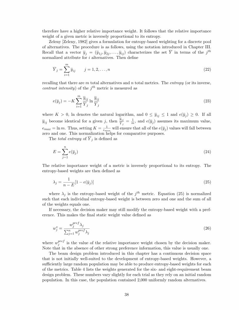
therefore have a higher relative importance weight. It follows that the relative importanceweight of a given metric is inversely proportional to its entropy.

Zeleny [Zeleny, 1982] gives a formulation for entropy-based weighting for a discrete poolof alternatives. The procedure is as follows, using the notation introduced in Chapter III.Recall that a vector yj = (y1j , y2j , . . . , yij) characterizes the set Y in terms of the jth

normalized attribute for i alternatives. Then define

Y j =m∑

i=1

yij j = 1, 2, . . . , n (22)

recalling that there are m total alternatives and n total metrics. The entropy (or its inverse,contrast intensity) of the jth metric is measured as

e(yj) = −Km∑

i=1

yij

Y j

lnyij

Y j

(23)

where K > 0, ln denotes the natural logarithm, and 0 ≤ yij ≤ 1 and e(yj) ≥ 0. If all

yij become identical for a given j, then yij

Y j= 1

m , and e(yj) assumes its maximum value,

emax = lnm. Thus, setting K = 1emax

will ensure that all of the e(yj) values will fall betweenzero and one. This normalization helps for comparative purposes.

The total entropy of Y j is defined as

E =n∑

j=1

e(yj) (24)

The relative importance weight of a metric is inversely proportional to its entropy. Theentropy-based weights are then defined as

λj =1

n− E[1− e(yj)] (25)

where λj is the entropy-based weight of the jth metric. Equation (25) is normalizedsuch that each individual entropy-based weight is between zero and one and the sum of allof the weights equals one.

If necessary, the decision maker may still modify the entropy-based weight with a pref-erence. This makes the final static weight value defined as

wsj =

wprefj λj∑n

j=1 wprefj λj

(26)

where wprefj is the value of the relative importance weight chosen by the decision maker.

Note that in the absence of other strong preference information, this value is usually one.The beam design problem introduced in this chapter has a continuous decision space

that is not initially well-suited to the development of entropy-based weights. However, asufficiently large random population may be able to produce entropy-based weights for eachof the metrics. Table 4 lists the weights generated for the six- and eight-requirement beamdesign problem. These numbers vary slightly for each trial as they rely on an initial randompopulation. In this case, the population contained 2,000 uniformly random alternatives.

38

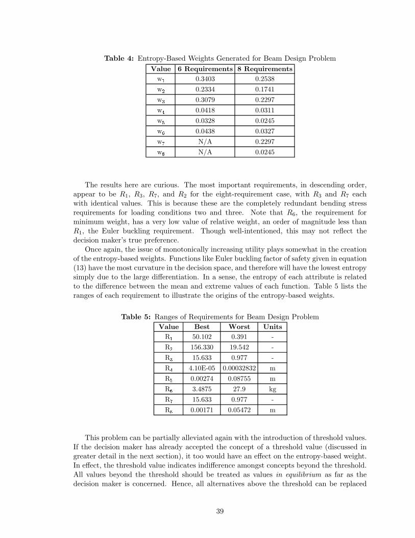
Table 4: Entropy-Based Weights Generated for Beam Design ProblemValue 6 Requirements 8 Requirementsw� 0.3403 0.2538w� 0.2334 0.1741w� 0.3079 0.2297w� 0.0418 0.0311w� 0.0328 0.0245w� 0.0438 0.0327w� N/A 0.2297w� N/A 0.0245

The results here are curious. The most important requirements, in descending order,appear to be R1, R3, R7, and R2 for the eight-requirement case, with R3 and R7 eachwith identical values. This is because these are the completely redundant bending stressrequirements for loading conditions two and three. Note that R6, the requirement forminimum weight, has a very low value of relative weight, an order of magnitude less thanR1, the Euler buckling requirement. Though well-intentioned, this may not reflect thedecision maker’s true preference.

Once again, the issue of monotonically increasing utility plays somewhat in the creationof the entropy-based weights. Functions like Euler buckling factor of safety given in equation(13) have the most curvature in the decision space, and therefore will have the lowest entropysimply due to the large differentiation. In a sense, the entropy of each attribute is relatedto the difference between the mean and extreme values of each function. Table 5 lists theranges of each requirement to illustrate the origins of the entropy-based weights.

Table 5: Ranges of Requirements for Beam Design ProblemValue Best Worst UnitsR� 50.102 0.391 -R� 156.330 19.542 -R� 15.633 0.977 -R� 4.10E-05 0.00032832 mR� 0.00274 0.08755 mR� 3.4875 27.9 kgR� 15.633 0.977 -R� 0.00171 0.05472 m

This problem can be partially alleviated again with the introduction of threshold values.If the decision maker has already accepted the concept of a threshold value (discussed ingreater detail in the next section), it too would have an effect on the entropy-based weight.In effect, the threshold value indicates indifference amongst concepts beyond the threshold.All values beyond the threshold should be treated as values in equilibrium as far as thedecision maker is concerned. Hence, all alternatives above the threshold can be replaced

39

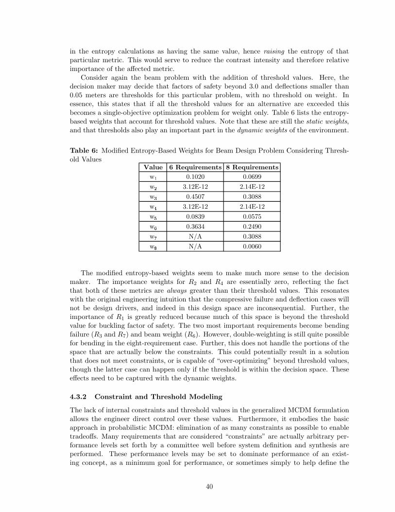
in the entropy calculations as having the same value, hence raising the entropy of thatparticular metric. This would serve to reduce the contrast intensity and therefore relativeimportance of the affected metric.

Consider again the beam problem with the addition of threshold values. Here, thedecision maker may decide that factors of safety beyond 3.0 and deflections smaller than0.05 meters are thresholds for this particular problem, with no threshold on weight. Inessence, this states that if all the threshold values for an alternative are exceeded thisbecomes a single-objective optimization problem for weight only. Table 6 lists the entropy-based weights that account for threshold values. Note that these are still the static weights,and that thresholds also play an important part in the dynamic weights of the environment.

Table 6: Modified Entropy-Based Weights for Beam Design Problem Considering Thresh-old Values

Value 6 Requirements 8 Requirementsw� 0.1020 0.0699w� 3.12E-12 2.14E-12w� 0.4507 0.3088w� 3.12E-12 2.14E-12w� 0.0839 0.0575w� 0.3634 0.2490w� N/A 0.3088w� N/A 0.0060

The modified entropy-based weights seem to make much more sense to the decisionmaker. The importance weights for R2 and R4 are essentially zero, reflecting the factthat both of these metrics are always greater than their threshold values. This resonateswith the original engineering intuition that the compressive failure and deflection cases willnot be design drivers, and indeed in this design space are inconsequential. Further, theimportance of R1 is greatly reduced because much of this space is beyond the thresholdvalue for buckling factor of safety. The two most important requirements become bendingfailure (R3 and R7) and beam weight (R6). However, double-weighting is still quite possiblefor bending in the eight-requirement case. Further, this does not handle the portions of thespace that are actually below the constraints. This could potentially result in a solutionthat does not meet constraints, or is capable of “over-optimizing” beyond threshold values,though the latter case can happen only if the threshold is within the decision space. Theseeffects need to be captured with the dynamic weights.

4.3.2 Constraint and Threshold Modeling

The lack of internal constraints and threshold values in the generalized MCDM formulationallows the engineer direct control over these values. Furthermore, it embodies the basicapproach in probabilistic MCDM: elimination of as many constraints as possible to enabletradeoffs. Many requirements that are considered “constraints” are actually arbitrary per-formance levels set forth by a committee well before system definition and synthesis areperformed. These performance levels may be set to dominate performance of an exist-ing concept, as a minimum goal for performance, or sometimes simply to help define the

40

problem better for typical single-objective optimization or fuel-balance sizing. Eliminationof these constraints is crucial to MCDM as it allows for implicit tradeoffs to be made onhigh-payoff objectives at the expense of less important objectives. However, some actualconstraints do exist, usually for safety, certification, or resource reasons. Several examplesof true constraints can be seen in meeting the Code of Federal Regulations for civil transportdesign [Federal Aviation Administration, 2005]. As such, the decision maker does need tobe able to input constraints into the MCDM environment.

The concept of threshold values was first introduced in the static weighting scheme.These are even more important for the dynamic portion of the weights if the threshold liessomewhere within the decision space. Beyond the threshold, improvement in the metricbecomes inconsequential. Modeling this behavior is crucial if the decision maker has athreshold in mind.

In a basic sense, the ideal dynamic weight will rise sharply if its associated constraintis violated. This makes it the most important objective in the space until the constraint issatisfied. At this point, the dynamic weight quickly drops to zero and the MCDM algorithmproceeds using only the static weight. If the metric improves much beyond its constraintand has a threshold value the dynamic weight will become slightly negative, becoming morenegative until it reaches the threshold value, upon which it is equal to exactly the oppositeof the static weight value. Therefore, the sum of the static and dynamic weights equalsexactly zero at or beyond the threshold, effectively negating any influence of that metric onthe MCDM algorithm.

Specifically, this dynamic weight cannot have too sharp of a change in value. If itwere too sharp it could increase the difficulty associated with gradient-based optimizers.Therefore, continuous, smooth functions should be used whenever possible. Further, thesedynamically modified weights should not be re-normalized to sum to one, else any change inone weight would change all others. This could also have an adverse effect on gradient-basedoptimizers.

The constraint portion of the dynamic weight model should approximate a step function.One attractive option is to find a smooth approximation of the Heaviside Step Function,also known as the Unit Step Function [Weisstein, 2005]. An approximation to this is definedas

wdcj (~x) = −1

[− 1

2+

1π

tan−1[s(yj(~x)− c)

]](27)

where wdcj refers to the constraint contribution to the jth dynamic weight, yj(~x) refers to

the current value of the jth metric, c refers to the normalized constraint value, and s is ascale factor for controlling smoothness of the step function. Larger values of s will make thestep function more abrupt. If s is too abrupt there may be problems with gradient-basedoptimizers, whereas if it is too small it will not jump fast enough near the constraint. Agood value of s is approximately 200, though this is best tailored to the individual problemsand optimization algorithms used.

The threshold value needs to have a more gradual decay, such as that seen in an inversepower relationship. It should be zero at the constraint value (or the edge of the designspace, if no constraint is present) and should be opposite of the static weighting value atthe threshold value. A good model for this is

wdtj (~x) = −ws

j

(1− t− yj(~x)

t− c

) 14

(28)

41

where wdtj is the threshold contribution to the jth dynamic weight and t is the normalized

threshold value. Note that both c and t should be normalized by the same procedure asresponse surface equations; that is, by the mean and variance of their respective responses.If c is less than -1.0 then the entire decision space is beyond the constraint; likewise for t. Ifeither value is greater than 1.0 it implies that the entire space is smaller than the constraintor threshold value.

Equations (27) and (28) can be combined into a single dynamic weight that is validacross the entire space no matter what its nature. This is represented by

wdj (~x) =

[12 − 1

π tan−1[s(yj(~x)− c)

]]− ws

j

(1− t−yj(~x)

t−c

) 14

yj(~x) ≤ t

−wsj yj(~x) > t

(29)

with the notation as noted before. A plot of an example dynamic weight function for allyj(~x) is given in Figure 22.

-1 -0.8 -0.6 -0.4 -0.2 0 0.2 0.4 0.6 0.8 1-0.4

-0.2

0

0.2

0.4

0.6

0.8

1

�

��

constraint threshold

w�

Figure 22: Example Dynamic Weight Variation with yj(~x)

4.3.3 Beam Design Problem with Dynamic Importance Weighting

The example beam design problem was reformulated with all of the concepts discussedin this section: entropy-based static weights with thresholds, augmented with dynamicweights with appropriate constraints and thresholds. The threshold values were as discussedearlier; all factors of safety were considered indifferent above 3.0 and all deflections below

42

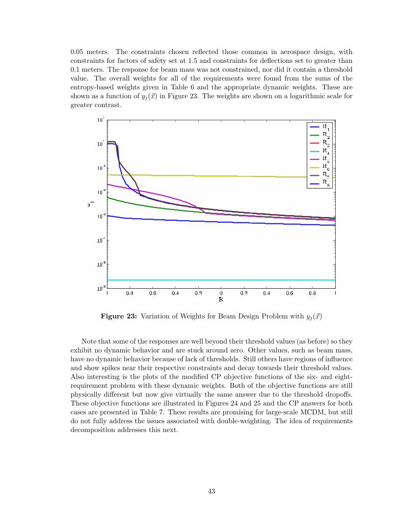
0.05 meters. The constraints chosen reflected those common in aerospace design, withconstraints for factors of safety set at 1.5 and constraints for deflections set to greater than0.1 meters. The response for beam mass was not constrained, nor did it contain a thresholdvalue. The overall weights for all of the requirements were found from the sums of theentropy-based weights given in Table 6 and the appropriate dynamic weights. These areshown as a function of yj(~x) in Figure 23. The weights are shown on a logarithmic scale forgreater contrast.

��

��

��

��

��

��

��

��

��

��

��

��

��

��

��

��

��

�

��

��

��

��

��

��

��

��

��

Figure 23: Variation of Weights for Beam Design Problem with yj(~x)

Note that some of the responses are well beyond their threshold values (as before) so theyexhibit no dynamic behavior and are stuck around zero. Other values, such as beam mass,have no dynamic behavior because of lack of thresholds. Still others have regions of influenceand show spikes near their respective constraints and decay towards their threshold values.Also interesting is the plots of the modified CP objective functions of the six- and eight-requirement problem with these dynamic weights. Both of the objective functions are stillphysically different but now give virtually the same answer due to the threshold dropoffs.These objective functions are illustrated in Figures 24 and 25 and the CP answers for bothcases are presented in Table 7. These results are promising for large-scale MCDM, but stilldo not fully address the issues associated with double-weighting. The idea of requirementsdecomposition addresses this next.

43

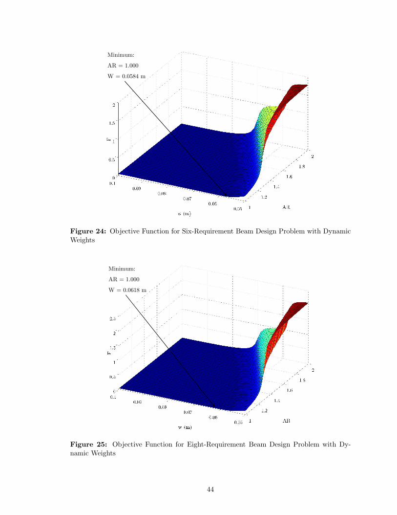
Minimum:AR = 1.000W = 0.0584 m

Figure 24: Objective Function for Six-Requirement Beam Design Problem with DynamicWeights

Minimum:AR = 1.000W = 0.0618 m

Figure 25: Objective Function for Eight-Requirement Beam Design Problem with Dy-namic Weights

44

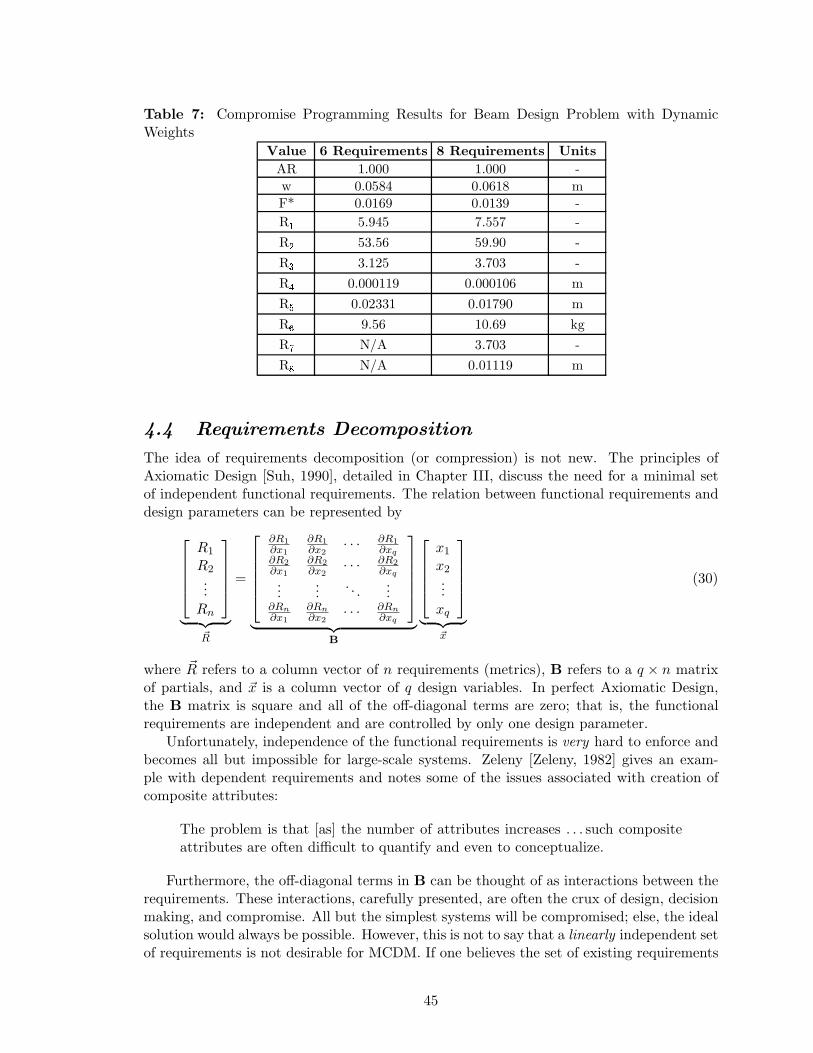
Table 7: Compromise Programming Results for Beam Design Problem with DynamicWeights

Value 6 Requirements 8 Requirements UnitsAR 1.000 1.000 -w 0.0584 0.0618 mF* 0.0169 0.0139 -R� 5.945 7.557 -R� 53.56 59.90 -R� 3.125 3.703 -R� 0.000119 0.000106 mR� 0.02331 0.01790 mR� 9.56 10.69 kgR� N/A 3.703 -R� N/A 0.01119 m

4.4 Requirements Decomposition

The idea of requirements decomposition (or compression) is not new. The principles ofAxiomatic Design [Suh, 1990], detailed in Chapter III, discuss the need for a minimal setof independent functional requirements. The relation between functional requirements anddesign parameters can be represented by

R1

R2...

Rn

︸︷︷︸~R

=

∂R1∂x1

∂R1∂x2

· · · ∂R1∂xq

∂R2∂x1

∂R2∂x2

· · · ∂R2∂xq

......

. . ....

∂Rn∂x1

∂Rn∂x2

· · · ∂Rn∂xq

︸︷︷︸B

x1

x2...

xq

︸︷︷︸~x

(30)

where ~R refers to a column vector of n requirements (metrics), B refers to a q × n matrixof partials, and ~x is a column vector of q design variables. In perfect Axiomatic Design,the B matrix is square and all of the off-diagonal terms are zero; that is, the functionalrequirements are independent and are controlled by only one design parameter.

Unfortunately, independence of the functional requirements is very hard to enforce andbecomes all but impossible for large-scale systems. Zeleny [Zeleny, 1982] gives an exam-ple with dependent requirements and notes some of the issues associated with creation ofcomposite attributes:

The problem is that [as] the number of attributes increases . . . such compositeattributes are often difficult to quantify and even to conceptualize.

Furthermore, the off-diagonal terms in B can be thought of as interactions between therequirements. These interactions, carefully presented, are often the crux of design, decisionmaking, and compromise. All but the simplest systems will be compromised; else, the idealsolution would always be possible. However, this is not to say that a linearly independent setof requirements is not desirable for MCDM. If one believes the set of existing requirements

45

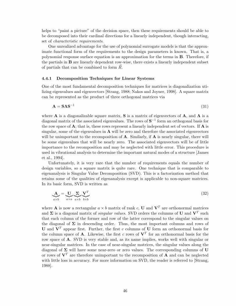
helps to “paint a picture” of the decision space, then these requirements should be able tobe decomposed into their cardinal directions for a linearly independent, though interacting,set of characteristic requirements.

One unrealized advantage for the use of polynomial surrogate models is that the approx-imate functional form of the requirements to the design parameters is known. That is, apolynomial response surface equation is an approximation for the terms in B. Therefore, ifthe partials in B are linearly dependent row-wise, there exists a linearly independent subsetof partials that can be combined to form ~R.

4.4.1 Decomposition Techniques for Linear Systems

One of the most fundamental decomposition techniques for matrices is diagonalization uti-lizing eigenvalues and eigenvectors [Strang, 1988; Nakos and Joyner, 1998]. A square matrixcan be represented as the product of three orthogonal matrices via

A = SΛS−1 (31)

where A is a diagonalizable square matrix, S is a matrix of eigenvectors of A, and Λ is adiagonal matrix of the associated eigenvalues. The rows of S−1 form an orthogonal basis forthe row space of A; that is, these rows represent a linearly independent set of vectors. If A issingular, some of the eigenvalues in Λ will be zero and therefore the associated eigenvectorswill be unimportant to the recomposition of A. Similarly, if A is nearly singular, there willbe some eigenvalues that will be nearly zero. The associated eigenvectors will be of littleimportance to the recomposition and may be neglected with little error. This procedure isused in vibrational analysis to determine the important natural modes of a structure [Jameset al., 1994].

Unfortunately, it is very rare that the number of requirements equals the number ofdesign variables, so a square matrix is quite rare. One technique that is comparable toeigenanalysis is Singular Value Decomposition (SVD). This is a factorization method thatretains some of the qualities of eigenanalysis except is applicable to non-square matrices.In its basic form, SVD is written as

A︸︷︷︸a×b

= U︸︷︷︸a×a

Σ︸︷︷︸a×b

VT︸︷︷︸b×b

(32)

where A is now a rectangular a× b matrix of rank c, U and VT are orthonormal matricesand Σ is a diagonal matrix of singular values. SVD orders the columns of U and VT suchthat each column of the former and row of the latter correspond to the singular values onthe diagonal of Σ in descending order. Thus, the most important columns and rows ofU and VT appear first. Further, the first c columns of U form an orthonormal basis forthe column space of A. Likewise, the first c rows of VT for an orthonormal basis for therow space of A. SVD is very stable and, as its name implies, works well with singular ornear-singular matrices. In the case of near-singular matrices, the singular values along thediagonal of Σ will have some near-zero or zero values. The corresponding columns of Uor rows of VT are therefore unimportant to the recomposition of A and can be neglectedwith little loss in accuracy. For more information on SVD, the reader is referred to [Strang,1988].

46

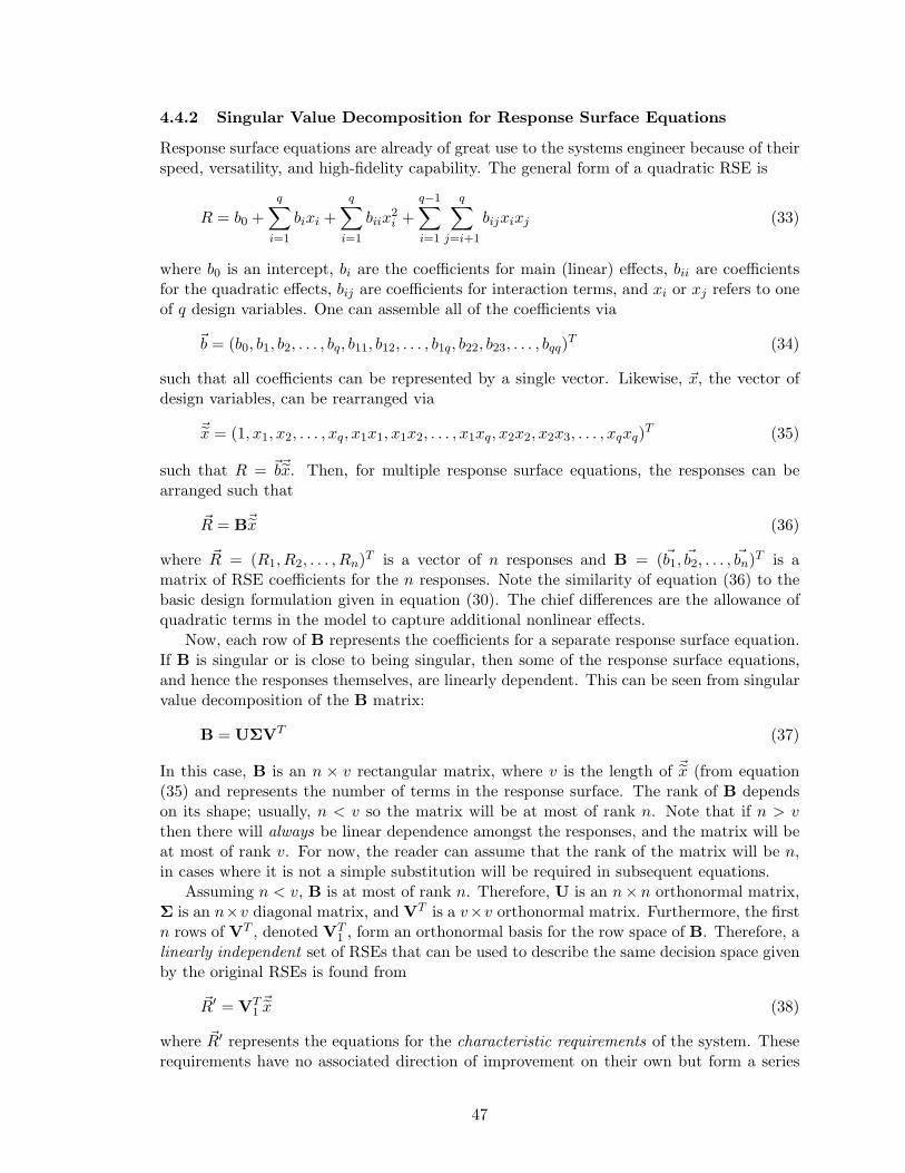
4.4.2 Singular Value Decomposition for Response Surface Equations

Response surface equations are already of great use to the systems engineer because of theirspeed, versatility, and high-fidelity capability. The general form of a quadratic RSE is

R = b0 +q∑

i=1

bixi +q∑

i=1

biix2i +

q−1∑

i=1

q∑

j=i+1

bijxixj (33)

where b0 is an intercept, bi are the coefficients for main (linear) effects, bii are coefficientsfor the quadratic effects, bij are coefficients for interaction terms, and xi or xj refers to oneof q design variables. One can assemble all of the coefficients via

~b = (b0, b1, b2, . . . , bq, b11, b12, . . . , b1q, b22, b23, . . . , bqq)T (34)

such that all coefficients can be represented by a single vector. Likewise, ~x, the vector ofdesign variables, can be rearranged via

~x = (1, x1, x2, . . . , xq, x1x1, x1x2, . . . , x1xq, x2x2, x2x3, . . . , xqxq)T (35)

such that R = ~b~x. Then, for multiple response surface equations, the responses can bearranged such that

~R = B~x (36)

where ~R = (R1, R2, . . . , Rn)T is a vector of n responses and B = (~b1, ~b2, . . . , ~bn)T is amatrix of RSE coefficients for the n responses. Note the similarity of equation (36) to thebasic design formulation given in equation (30). The chief differences are the allowance ofquadratic terms in the model to capture additional nonlinear effects.

Now, each row of B represents the coefficients for a separate response surface equation.If B is singular or is close to being singular, then some of the response surface equations,and hence the responses themselves, are linearly dependent. This can be seen from singularvalue decomposition of the B matrix:

B = UΣVT (37)

In this case, B is an n × v rectangular matrix, where v is the length of ~x (from equation(35) and represents the number of terms in the response surface. The rank of B dependson its shape; usually, n < v so the matrix will be at most of rank n. Note that if n > vthen there will always be linear dependence amongst the responses, and the matrix will beat most of rank v. For now, the reader can assume that the rank of the matrix will be n,in cases where it is not a simple substitution will be required in subsequent equations.

Assuming n < v, B is at most of rank n. Therefore, U is an n× n orthonormal matrix,Σ is an n×v diagonal matrix, and VT is a v×v orthonormal matrix. Furthermore, the firstn rows of VT , denoted VT

1 , form an orthonormal basis for the row space of B. Therefore, alinearly independent set of RSEs that can be used to describe the same decision space givenby the original RSEs is found from

~R′ = VT1~x (38)

where ~R′ represents the equations for the characteristic requirements of the system. Theserequirements have no associated direction of improvement on their own but form a series

47

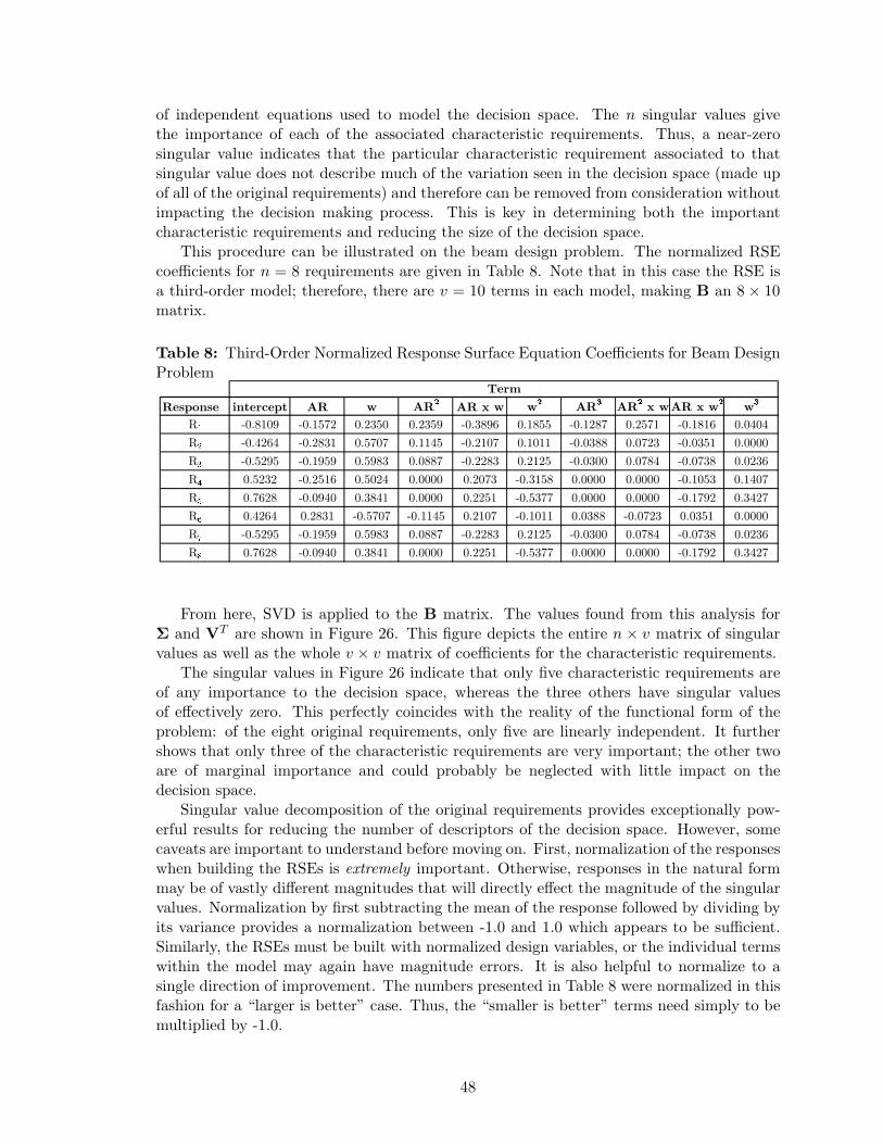
of independent equations used to model the decision space. The n singular values givethe importance of each of the associated characteristic requirements. Thus, a near-zerosingular value indicates that the particular characteristic requirement associated to thatsingular value does not describe much of the variation seen in the decision space (made upof all of the original requirements) and therefore can be removed from consideration withoutimpacting the decision making process. This is key in determining both the importantcharacteristic requirements and reducing the size of the decision space.

This procedure can be illustrated on the beam design problem. The normalized RSEcoefficients for n = 8 requirements are given in Table 8. Note that in this case the RSE isa third-order model; therefore, there are v = 10 terms in each model, making B an 8× 10matrix.

Table 8: Third-Order Normalized Response Surface Equation Coefficients for Beam DesignProblem

Response intercept AR w AR�

AR x w w�

AR�

AR�

x wAR x w�

w�

R� -0.8109 -0.1572 0.2350 0.2359 -0.3896 0.1855 -0.1287 0.2571 -0.1816 0.0404R� -0.4264 -0.2831 0.5707 0.1145 -0.2107 0.1011 -0.0388 0.0723 -0.0351 0.0000R� -0.5295 -0.1959 0.5983 0.0887 -0.2283 0.2125 -0.0300 0.0784 -0.0738 0.0236R� 0.5232 -0.2516 0.5024 0.0000 0.2073 -0.3158 0.0000 0.0000 -0.1053 0.1407R� 0.7628 -0.0940 0.3841 0.0000 0.2251 -0.5377 0.0000 0.0000 -0.1792 0.3427R� 0.4264 0.2831 -0.5707 -0.1145 0.2107 -0.1011 0.0388 -0.0723 0.0351 0.0000R� -0.5295 -0.1959 0.5983 0.0887 -0.2283 0.2125 -0.0300 0.0784 -0.0738 0.0236R 0.7628 -0.0940 0.3841 0.0000 0.2251 -0.5377 0.0000 0.0000 -0.1792 0.3427

Term

From here, SVD is applied to the B matrix. The values found from this analysis forΣ and VT are shown in Figure 26. This figure depicts the entire n × v matrix of singularvalues as well as the whole v × v matrix of coefficients for the characteristic requirements.

The singular values in Figure 26 indicate that only five characteristic requirements areof any importance to the decision space, whereas the three others have singular valuesof effectively zero. This perfectly coincides with the reality of the functional form of theproblem: of the eight original requirements, only five are linearly independent. It furthershows that only three of the characteristic requirements are very important; the other twoare of marginal importance and could probably be neglected with little impact on thedecision space.

Singular value decomposition of the original requirements provides exceptionally pow-erful results for reducing the number of descriptors of the decision space. However, somecaveats are important to understand before moving on. First, normalization of the responseswhen building the RSEs is extremely important. Otherwise, responses in the natural formmay be of vastly different magnitudes that will directly effect the magnitude of the singularvalues. Normalization by first subtracting the mean of the response followed by dividing byits variance provides a normalization between -1.0 and 1.0 which appears to be sufficient.Similarly, the RSEs must be built with normalized design variables, or the individual termswithin the model may again have magnitude errors. It is also helpful to normalize to asingle direction of improvement. The numbers presented in Table 8 were normalized in thisfashion for a “larger is better” case. Thus, the “smaller is better” terms need simply to bemultiplied by -1.0.

48

��

� ��

� � ��

� � � ��

� � � � ��

� � � � � ��

� � � � � � ��

� � � � � � � ��

��

��

��

��

��

��

��

��

��

��

� ��

��

��

��

��

��

��

��

��

��

��

��

��

��

��

��

��

��

��

��

��

��

��

��

��

��

��

��

��

��

� ��

��

��

��

��

��

��

��

��

��

��

��

��

��

��

��

��

��

��

��

� ��

��

��

��

��

��

��

��

��

��

��

��

��

��

��

��

��

��

��

��

��

��

��

��

��

��

��

��

��

��

� ��

��

��

��

��

��

��

��

��

��

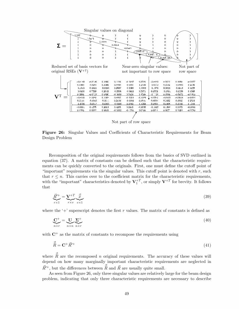
ΣΣΣΣ =

VT =

Not part of row space

Not part of row space

Singular values on diagonal

Near-zero singular values: not important to row space

Reduced set of basis vectors for original RSEs (V+T)

Figure 26: Singular Values and Coefficients of Characteristic Requirements for BeamDesign Problem

Recomposition of the original requirements follows from the basics of SVD outlined inequation (37). A matrix of constants can be defined such that the characteristic require-ments can be quickly converted to the originals. First, one must define the cutoff point of“important” requirements via the singular values. This cutoff point is denoted with r, suchthat r ≤ n. This carries over to the coefficient matrix for the characteristic requirements,with the “important” characteristics denoted by V+T

1 , or simply V+T for brevity. It followsthat

~R′+︸︷︷︸r×1

= V+T︸︷︷︸r×v

~x︸︷︷︸v×1

(39)

where the ‘+’ superscript denotes the first r values. The matrix of constants is defined as

C+︸︷︷︸n×r

= U︸︷︷︸n×n

Σ+︸︷︷︸n×r

(40)

with C+ as the matrix of constants to recompose the requirements using

~R = C+ ~R′+ (41)

where ~R are the recomposed n original requirements. The accuracy of these values will

depend on how many marginally important characteristic requirements are neglected in~R′+, but the differences between ~

R and ~R are usually quite small.As seen from Figure 26, only three singular values are relatively large for the beam design

problem, indicating that only three characteristic requirements are necessary to describe

49

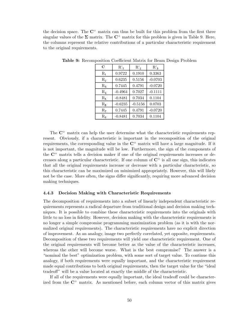
the decision space. The C+ matrix can thus be built for this problem from the first threesingular values of the Σ matrix. The C+ matrix for this problem is given in Table 9. Here,the columns represent the relative contributions of a particular characteristic requirementto the original requirements.

Table 9: Recomposition Coefficient Matrix for Beam Design Problem�� R'� R'� R'�R� 0.9722 0.1910 0.3363R� 0.6235 0.5156 -0.0703R� 0.7445 0.4791 -0.0720R� -0.4964 0.7027 -0.1111R� -0.8481 0.7034 0.1104R� -0.6235 -0.5156 0.0703R� 0.7445 0.4791 -0.0720R -0.8481 0.7034 0.1104

The C+ matrix can help the user determine what the characteristic requirements rep-resent. Obviously, if a characteristic is important in the recomposition of the originalrequirements, the corresponding value in the C+ matrix will have a large magnitude. If itis not important, the magnitude will be low. Furthermore, the sign of the components ofthe C+ matrix tells a decision maker if one of the original requirements increases or de-creases along a particular characteristic. If one column of C+ is all one sign, this indicatesthat all the original requirements increase or decrease with a particular characteristic, sothis characteristic can be maximized on minimized appropriately. However, this will likelynot be the case. More often, the signs differ significantly, requiring more advanced decisionmaking techniques.

4.4.3 Decision Making with Characteristic Requirements

The decomposition of requirements into a subset of linearly independent characteristic re-quirements represents a radical departure from traditional design and decision making tech-niques. It is possible to combine these characteristic requirements into the originals withlittle to no loss in fidelity. However, decision making with the characteristic requirements isno longer a simple compromise programming maximization problem (as it is with the nor-malized original requirements). The characteristic requirements have no explicit directionof improvement. As an analogy, image two perfectly correlated, yet opposite, requirements.Decomposition of these two requirements will yield one characteristic requirement. One ofthe original requirements will become better as the value of the characteristic increases,whereas the other will become worse. What is the best compromise? The answer is a“nominal the best” optimization problem, with some sort of target value. To continue thisanalogy, if both requirements were equally important, and the characteristic requirementmade equal contributions to both original requirements, then the target value for the “idealtradeoff” will be a value located at exactly the middle of the characteristic.

If all of the requirements were equally important, the ideal tradeoff could be character-ized from the C+ matrix. As mentioned before, each column vector of this matrix gives

50

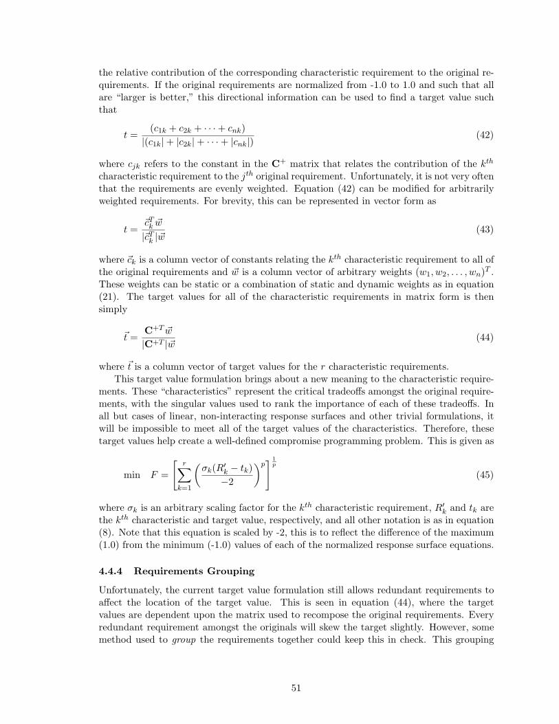
the relative contribution of the corresponding characteristic requirement to the original re-quirements. If the original requirements are normalized from -1.0 to 1.0 and such that allare “larger is better,” this directional information can be used to find a target value suchthat

t =(c1k + c2k + · · ·+ cnk)

|(c1k|+ |c2k|+ · · ·+ |cnk|) (42)

where cjk refers to the constant in the C+ matrix that relates the contribution of the kth

characteristic requirement to the jth original requirement. Unfortunately, it is not very oftenthat the requirements are evenly weighted. Equation (42) can be modified for arbitrarilyweighted requirements. For brevity, this can be represented in vector form as

t =~cT

k ~w

|~cTk |~w

(43)

where ~ck is a column vector of constants relating the kth characteristic requirement to all ofthe original requirements and ~w is a column vector of arbitrary weights (w1, w2, . . . , wn)T .These weights can be static or a combination of static and dynamic weights as in equation(21). The target values for all of the characteristic requirements in matrix form is thensimply

~t =C+T ~w

|C+T |~w (44)

where ~t is a column vector of target values for the r characteristic requirements.This target value formulation brings about a new meaning to the characteristic require-

ments. These “characteristics” represent the critical tradeoffs amongst the original require-ments, with the singular values used to rank the importance of each of these tradeoffs. Inall but cases of linear, non-interacting response surfaces and other trivial formulations, itwill be impossible to meet all of the target values of the characteristics. Therefore, thesetarget values help create a well-defined compromise programming problem. This is given as

min F =

[r∑

k=1

(σk(R′

k − tk)−2

)p] 1

p

(45)

where σk is an arbitrary scaling factor for the kth characteristic requirement, R′k and tk are

the kth characteristic and target value, respectively, and all other notation is as in equation(8). Note that this equation is scaled by -2, this is to reflect the difference of the maximum(1.0) from the minimum (-1.0) values of each of the normalized response surface equations.

4.4.4 Requirements Grouping

Unfortunately, the current target value formulation still allows redundant requirements toaffect the location of the target value. This is seen in equation (44), where the targetvalues are dependent upon the matrix used to recompose the original requirements. Everyredundant requirement amongst the originals will skew the target slightly. However, somemethod used to group the requirements together could keep this in check. This grouping

51

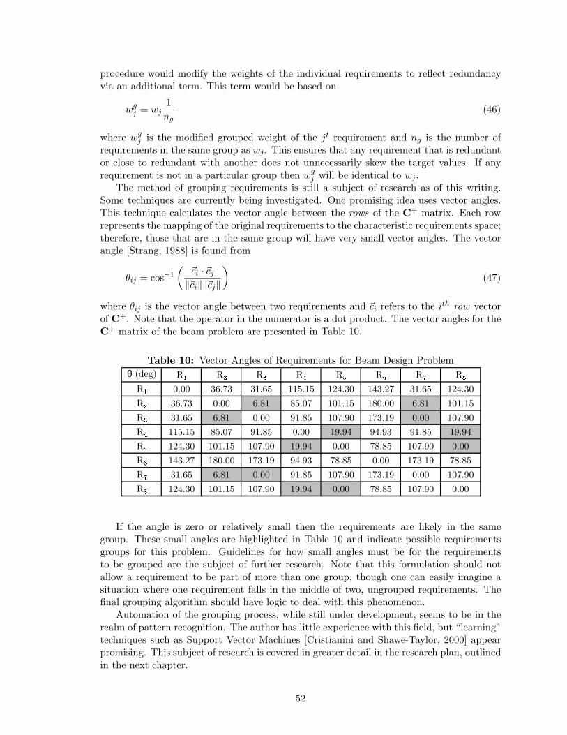
procedure would modify the weights of the individual requirements to reflect redundancyvia an additional term. This term would be based on

wgj = wj

1ng

(46)

where wgj is the modified grouped weight of the jt requirement and ng is the number of

requirements in the same group as wj . This ensures that any requirement that is redundantor close to redundant with another does not unnecessarily skew the target values. If anyrequirement is not in a particular group then wg

j will be identical to wj .The method of grouping requirements is still a subject of research as of this writing.

Some techniques are currently being investigated. One promising idea uses vector angles.This technique calculates the vector angle between the rows of the C+ matrix. Each rowrepresents the mapping of the original requirements to the characteristic requirements space;therefore, those that are in the same group will have very small vector angles. The vectorangle [Strang, 1988] is found from

θij = cos−1

(~ci · ~cj

‖~ci‖‖~cj‖)

(47)

where θij is the vector angle between two requirements and ~ci refers to the ith row vectorof C+. Note that the operator in the numerator is a dot product. The vector angles for theC+ matrix of the beam problem are presented in Table 10.

Table 10: Vector Angles of Requirements for Beam Design Problemθ (deg) R� R� R� R� R� R� R� R�

R� 0.00 36.73 31.65 115.15 124.30 143.27 31.65 124.30R� 36.73 0.00 6.81 85.07 101.15 180.00 6.81 101.15R� 31.65 6.81 0.00 91.85 107.90 173.19 0.00 107.90R� 115.15 85.07 91.85 0.00 19.94 94.93 91.85 19.94R� 124.30 101.15 107.90 19.94 0.00 78.85 107.90 0.00R� 143.27 180.00 173.19 94.93 78.85 0.00 173.19 78.85R� 31.65 6.81 0.00 91.85 107.90 173.19 0.00 107.90R� 124.30 101.15 107.90 19.94 0.00 78.85 107.90 0.00

If the angle is zero or relatively small then the requirements are likely in the samegroup. These small angles are highlighted in Table 10 and indicate possible requirementsgroups for this problem. Guidelines for how small angles must be for the requirementsto be grouped are the subject of further research. Note that this formulation should notallow a requirement to be part of more than one group, though one can easily imagine asituation where one requirement falls in the middle of two, ungrouped requirements. Thefinal grouping algorithm should have logic to deal with this phenomenon.

Automation of the grouping process, while still under development, seems to be in therealm of pattern recognition. The author has little experience with this field, but “learning”techniques such as Support Vector Machines [Cristianini and Shawe-Taylor, 2000] appearpromising. This subject of research is covered in greater detail in the research plan, outlinedin the next chapter.

52

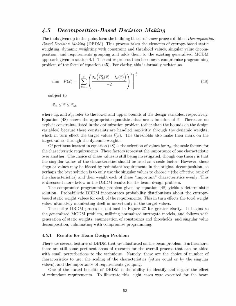
4.5 Decomposition-Based Decision Making

The tools given up to this point form the building blocks of a new process dubbed Decomposition-Based Decision Making (DBDM). This process takes the elements of entropy-based staticweighting, dynamic weighting with constraint and threshold values, singular value decom-position, and requirements grouping and adds them to the existing generalized MCDMapproach given in section 4.1. The entire process then becomes a compromise programmingproblem of the form of equation (45). For clarity, this is formally written as

min F (~x) =

r∑

k=1

σk

(R′

k(~x)− tk(~x))

−2

p

1p

(48)

subject to

~xlb ≤ ~x ≤ ~xub

where ~xlb and ~xub refer to the lower and upper bounds of the design variables, respectively.Equation (48) shows the appropriate quantities that are a function of ~x. There are noexplicit constraints listed in the optimization problem (other than the bounds on the designvariables) because these constraints are handled implicitly through the dynamic weights,which in turn effect the target values ~t(~x). The thresholds also make their mark on thetarget values through the dynamic weights.

Of pertinent interest in equation (48) is the selection of values for σk, the scale factors forthe characteristic requirements. These factors represent the importance of one characteristicover another. The choice of these values is still being investigated, though one theory is thatthe singular values of the characteristics should be used as a scale factor. However, thesesingular values may be biased by redundant requirements in the original decomposition, soperhaps the best solution is to only use the singular values to choose r (the effective rank ofthe characteristics) and then weight each of these “important” characteristics evenly. Thisis discussed more below in the DBDM results for the beam design problem.

The compromise programming problem given by equation (48) yields a deterministicsolution. Probabilistic DBDM incorporates probability distributions about the entropy-based static weight values for each of the requirements. This in turn effects the total weightvalue, ultimately manifesting itself in uncertainty in the target values.

The entire DBDM process is outlined in Figure 27 for greater clarity. It begins asthe generalized MCDM problem, utilizing normalized surrogate models, and follows withgeneration of static weights, enumeration of constraints and thresholds, and singular valuedecomposition, culminating with compromise programming.

4.5.1 Results for Beam Design Problem

There are several features of DBDM that are illustrated on the beam problem. Furthermore,there are still some pertinent areas of research for the overall process that can be aidedwith small perturbations to the technique. Namely, these are the choice of number ofcharacteristics to use, the scaling of the characteristics (either equal or by the singularvalues), and the importance of requirements grouping.

One of the stated benefits of DBDM is the ability to identify and negate the effectof redundant requirements. To illustrate this, eight cases were executed for the beam

53

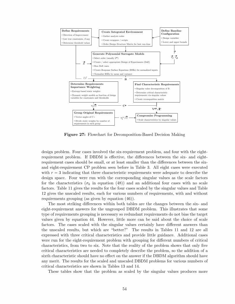
Define Requirements• Direction of Improvement• List true constraints, if any• Determine threshold values

Create Integrated Environment• Gather analysis codes• Create wrappers / scripts• Order Design Structure Matrix for best run-time

Generate Polynomial Surrogate Models• Select order (usually 2��)• Create / select appropriate Design of Experiments (DoE)• Run DoE cases• Create Response Surface Equations (RSEs) for normalized inputs• Normalize RSEs by mean and variance

Determine Requirements Importance Weighting• Entropy-based static weights• Dynamic weight models as function of design variables for constraints and thresholds

Find Characteristic Requirements• Singular value decomposition of B• Determine critical characteristic requirements via singular values• Create recomposition matrix

Group Original Requirements• Vector angles of C+• Divide static weights by number of requirements in each group

Compromise Programming• Scale characteristics by singular values

Define Baseline Configuration• Design variables• Lower and upper bounds

xx��, x��

B

R

c,t

w��(x)

w�(x) C�V��, ΣΣΣΣ+

Figure 27: Flowchart for Decomposition-Based Decision Making

design problem. Four cases involved the six-requirement problem, and four with the eight-requirement problem. If DBDM is effective, the differences between the six- and eight-requirement cases should be small, or at least smaller than the differences between the six-and eight-requirement CP problem seen before in Table 3. All eight cases were executedwith r = 3 indicating that three characteristic requirements were adequate to describe thedesign space. Four were run with the corresponding singular values as the scale factorsfor the characteristics (σk in equation (48)) and an additional four cases with no scalefactors. Table 11 gives the results for the four cases scaled by the singular values and Table12 gives the unscaled results, each for various numbers of requirements, with and withoutrequirements grouping (as given by equation (46)).

The most striking differences within both tables are the changes between the six- andeight-requirement answers for the ungrouped DBDM problem. This illustrates that sometype of requirements grouping is necessary so redundant requirements do not bias the targetvalues given by equation 44. However, little more can be said about the choice of scalefactors. The cases scaled with the singular values certainly have different answers thanthe unscaled results, but which are “better?” The results in Tables 11 and 12 are allexpressed with three critical characteristics and provide little guidance. Additional caseswere run for the eight-requirement problem with grouping for different numbers of criticalcharacteristics, from two to six. Note that the reality of the problem shows that only fivecritical characteristics are needed to completely describe the problem, so the addition of asixth characteristic should have no effect on the answer if the DBDM algorithm should haveany merit. The results for the scaled and unscaled DBDM problems for various numbers ofcritical characteristics are shown in Tables 13 and 14.

These tables show that the problem as scaled by the singular values produces more

54

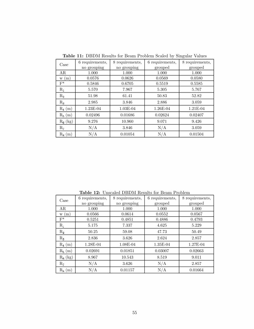
Table 11: DBDM Results for Beam Problem Scaled by Singular Values

Case 6 requirements, no grouping

8 requirements, no grouping

6 requirements, grouped


AR 1.000 1.000 1.000 1.000w (m) 0.0576 0.0626 0.0569 0.0580F* 0.5846 0.6705 0.5519 0.5585R� 5.570 7.967 5.305 5.767R� 51.98 61.41 50.83 52.82R� 2.985 3.846 2.886 3.059R� (m) 1.23E-04 1.03E-04 1.26E-04 1.21E-04R� (m) 0.02496 0.01686 0.02624 0.02407R� (kg) 9.276 10.960 9.071 9.426R� N/A 3.846 N/A 3.059R� (m) N/A 0.01054 N/A 0.01504

Table 12: Unscaled DBDM Results for Beam Problem

Case 6 requirements, no grouping

8 requirements, no grouping



AR 1.000 1.000 1.000 1.000w (m) 0.0566 0.0614 0.0552 0.0567F* 0.5251 0.4851 0.4886 0.4793R� 5.175 7.337 4.625 5.229R� 50.25 59.08 47.73 50.49R� 2.836 3.626 2.624 2.857R� (m) 1.28E-04 1.08E-04 1.35E-04 1.27E-04R� (m) 0.02691 0.01851 0.03007 0.02663R� (kg) 8.967 10.543 8.519 9.011R� N/A 3.626 N/A 2.857R� (m) N/A 0.01157 N/A 0.01664

55

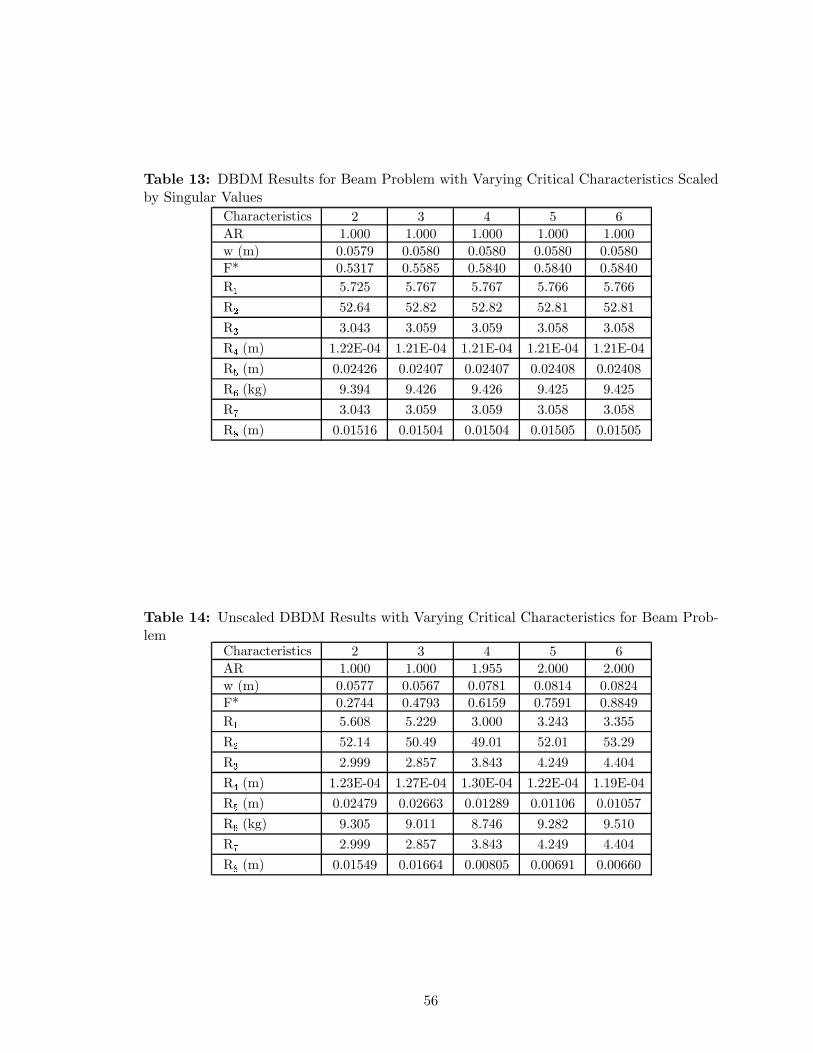
Table 13: DBDM Results for Beam Problem with Varying Critical Characteristics Scaledby Singular Values

Characteristics 2 3 4 5 6AR 1.000 1.000 1.000 1.000 1.000w (m) 0.0579 0.0580 0.0580 0.0580 0.0580F* 0.5317 0.5585 0.5840 0.5840 0.5840R� 5.725 5.767 5.767 5.766 5.766R� 52.64 52.82 52.82 52.81 52.81R� 3.043 3.059 3.059 3.058 3.058R� (m) 1.22E-04 1.21E-04 1.21E-04 1.21E-04 1.21E-04R� (m) 0.02426 0.02407 0.02407 0.02408 0.02408R� (kg) 9.394 9.426 9.426 9.425 9.425R� 3.043 3.059 3.059 3.058 3.058R� (m) 0.01516 0.01504 0.01504 0.01505 0.01505

Table 14: Unscaled DBDM Results with Varying Critical Characteristics for Beam Prob-lem

Characteristics 2 3 4 5 6AR 1.000 1.000 1.955 2.000 2.000w (m) 0.0577 0.0567 0.0781 0.0814 0.0824F* 0.2744 0.4793 0.6159 0.7591 0.8849R� 5.608 5.229 3.000 3.243 3.355R� 52.14 50.49 49.01 52.01 53.29R� 2.999 2.857 3.843 4.249 4.404R� (m) 1.23E-04 1.27E-04 1.30E-04 1.22E-04 1.19E-04R� (m) 0.02479 0.02663 0.01289 0.01106 0.01057R� (kg) 9.305 9.011 8.746 9.282 9.510R� 2.999 2.857 3.843 4.249 4.404R� (m) 0.01549 0.01664 0.00805 0.00691 0.00660

56

consistent answers, whereas the unscaled problem changes dramatically as the number ofcritical characteristics increases. Furthermore, the unscaled problem shows changes at r =6 critical characteristics, which is not physical since the problem only has five linearlyindependent requirements. Thus, it appears that the scaled problem should be the mostaccurate formulation.

4.6 Directions for Large-Scale Decision Making

The formulation for Decomposition-Based Decision Making is still evolving as this researchprogresses, but the results seem to resolve or circumvent the issues associated with gen-eralized MCDM applied to large systems. Preliminary studies using the example beamdesign problem indicate that the formulation given in equation (48) seems to work bestwhen scaled by the singular values and combined with a requirements grouping technique.Of these, the algorithm used for requirements grouping and the tolerance regarding how“close” requirements must be in order to belong to the same group are a matter of muchdebate. Still, the initial results are promising for DBDM. The pertinent features include:

• Polynomial surrogate models of the responses normalized by their mean and variance;

• Static weighting values determined by the threshold-modified “entropy” of the decisionspace;

• Dynamic weighting with the allowance for constraint and threshold values (implicitutility);

• Singular value decomposition of the decision space to identify the characteristic re-quirements which form the key tradeoffs of the system;

• Ideal tradeoff targets based on the relative contribution of the original requirementsto the characteristics;

• Grouping of the original requirements to eliminate double-weighting;

• Compromise programming to find the solution closest to the ideal tradeoff in thecharacteristic decision space scaled by the singular values of these characteristics.

These features should enable a decision maker to determine the best tradeoff solutionfor a large-scale multicriteria problem. Ultimately, this method can be made probabilisticto handle uncertainty in the requirements. This uncertainty can be manifested with prob-ability distributions about the static weight values, which in turn cascade into compromiseprogramming problem via the target values. The solution that is most robust with respectto changes in the importance of the metrics will in turn be the solution best suited touncertain requirements.

57

Bibliography

AIAA Technical Activities Committee. Current state of the art on multidisciplinary designoptimization (MDO). AIAA White Paper, 1991.

Asimow, Morris. Introduction to Design. Prentice-Hall, Englewood Cliffs, New Jersey, 1962.

Baker, Andrew P. The Role of Mission Requirements, Vehicle Attributes, Technologies andUncertainty in Rotorcraft System Design. Ph.D. thesis, Georgia Institute of Technology,Atlanta, Georgia, 2002.

Baker, Andrew P. and Mavris, Dimitri N. Assessing the simultaneous impact of require-ments, vehicle characteristics, and technologies during aircraft design. 2001-0533. 39thAerospace Sciences Meeting and Exhibit, American Institute of Aeronautics and Astro-nautics, 2001.

Bandte, Oliver. A Probabilistic Multi-Criteria Decision Making Technique for Conceptualand Preliminary Aerospace Systems Design. Ph.D. thesis, Georgia Institute of Technology,Atlanta, Georgia, 2000.

Baugher, Jay. USAAC / USAAF / USAF bomber aircraft. 2005. http://home.att.net/jbaugher/usafbombers.html.

Borer, Nicholas K. and Mavris, Dimitri N. Requirements exploration for a notional multi-role fighter. 2003-6709. 3rd Aviation Technology, Integration, and Operations TechnicalForum, American Institute of Aeronautics and Astronautics, 2003.

Borer, Nicholas K. and Mavris, Dimitri N. Formulation of a multi-mission sizing method-ology for competing configurations. 2004-0535. 42nd Aerospace Sciences Meeting andExhibit, American Institute of Aeronautics and Astronautics, 2004.

Brassard, Michael and Ritter, Diane. The Memory Jogger II. GOAL / QPC, Salem, NewHampshire, 1994.

Braun, Robert, Gage, Peter, and Kroo, Ilan. Implementation and performance issues incollaborative optimization. 96-4017. 6th Symposium on Multidisciplinary Analysis andOptimization, American Institute of Aeronautics and Astronautics, 1996.

Carty, A. An approach to multidisciplinary design, analysis, and optimization for rapidconceptual design. 2002-5438. 9th Symposium on Multidisciplinary Analysis and Opti-mization, American Institute of Aeronautics and Astronautics, Atlanta, Georgia, 2002.

Chvatal, Vasek. Linear Programming. W. H. Freeman and Company, New York, New York,1983.

Cristianini, Nello and Shawe-Taylor, John. An Introduction to Support Vector Machnies andOther Kernel-Based Learning Methods. Cambridge University Press, Cambridge, UnitedKingdom, 2000.

Czysz, P. A., Dighton, R. D., and W. P. Murden, Jr. Designing for air superiority. TechnicalReport 73-0800, McDonnell Aircraft Company, 1973.

58

Deb, Kalyanmoy. Multi-Objective Optimization using Evolutionary Algorithms. John Wileyand Sons, Chichester, England, 2001.

DeLaurentis, D., Mavris, D. N., and Schrage, D. P. System synthesis in preliminary air-craft design using statistical methods. 20th Congress of the International Council of theAeronautical Sciences, International Council of the Aeronautical Sciences, Sorrento, Italy,1996.

Department of the Navy. Navy historical center, naval aviation history branch. 2005.http://www.history.navy.mil/branches/nhcorg4.htm.

Dieter, George E. Engineering Design: A Meterials and Processing Approach, Third Edition.McGraw-Hill, Inc., Boston, Massachusetts, 2000.

Eckels, W. E. Civil transport aircraft design methodology. 83-2463. Aircraft Design, Sys-tems and Technology Meeting, American Institute of Aeronautics and Astronautics, FortWorth, Texas, 1983.

Engineous Software. iSIGHT - integrate, automate, and optimize your manual design pro-cesses. 2005. http://www.engineous.com/product iSIGHT.htm.

Federal Aviation Administration. Code of federal regulations, title 14,part 25: Airworthiness standards: Transport category airplanes. 2005.http://ecfr.gpoaccess.gov/cgi/t/text/text-idx?&c=ecfr&tpl=/ecfrbrowse/Title14/14tab02.tpl.

Federation of American Scientists. U.S. military aircraft. 2005.http://www.fas.org/man/dod-101/sys/ac/index.html.

Fox, Eric P. The Pratt and Whitney probabilistic design system. 94-1442. 35th Structures,Structural Dynamics, and Materials Conference, American Institute of Aeronautics andAstronautics, 1994.

Gerhards, Roland, Meller, Frank, Dirks, Gregor A., and Szodruch, Joachim. Aircraft designoptimizing operators, environmental system and manufacturers requirements. 2000-01-5546. 2000 World Aviation Congress, Society of Automotive Engineers, 2000.

Greenway, M. K. and Koob, S. J. Relating take-off-gross-weight and mission requirementsto geometrically optimized aircraft. 78-0098. 16th Aerospace Sciences Meeting, AmericanInstitute of Aeronautics and Astronautics, 1978.

Guynn, M. D. and Olson, E. D. Evaluation of an aircraft concept with over-wing, hydrogen-fueled engines for reduced noise and emissions. Technical Report TM-2002-211926, Na-tional Aeronautics and Space Administration, Hampton, Virginia, 2002.

Hibbeler, R. C. Mechanics of Materials, Third Edition. Prentice Hall, Upper Saddle River,New Jersey, 1997.

Hwang, Ching-Lai and Masud, Abu Syed Md. Multiple Objective Decision Making: Methodsand Applications. Lecture Notes in Economics and Mathematical Systems. Springer-Verlag, Berlin, Germany, 1979.

59

Hwang, Ching-Lai and Yoon, Kwangsun. Multiple Attirbute Decision Making: Methods andApplications. Lecture Notes in Economics and Mathematical Systems. Springer-Verlag,Berlin, Germany, 1981.

Ismail-Yahaya, Amir and Messac, Achille. Effective generation of the pareto frontier: Thenormalized normal constraint method. 2002-1232. 43rd Structures, Structural Dynamics,and Materials Conference, American Institute of Aeronautics and Astronautics, 2002.

James, M. L., Smith, G. M., Wolford, J. C., and Whaley, P. W. Vibration of Mechanical andStructural Systems: With Microcomputer Applications, Second Edition. HarperCollinsCollege Publishers, New York, New York, 1994.

Joy, D. P. and Simonds, R. M. The Rf graphical method of parametric analysis for thedevelopment of optimum preliminary design aircraft. Technical Report 107, AdvancedResearch Division of Hiller Helicopters, 1956.

Kam, J. Vander and Gage, P. The launch vehicle language (LVL) data model for evalu-ating reusable launch vehicle concepts. 2003-1330. 41st Aerospace Sciences Meeting andExhibit, American Institute of Aeronautics and Astronautics, Reno, Nevada, 2003.

Kirby, M. R. and Mavris, D. N. Forecasting technology uncertainty in preliminary aircraftdesign. 1999-01-5631. 1999 World Aviation Conference, Society of Automotive Engineers,San Francisco, California, 1999.

Kirby, M. R. and Mavris, D. N. An approach for the intelligent assessment of futuretechnology portfolios. 2002-0515. 40th Aerospace Sciences Meeting and Exhibit, AmericanInstitute of Aeronautics and Astronautics, Reno, Nevada, 2002.

Ledsinger, L. A. and Olds, J. R. Multidisciplinary design optimization techniques for branch-ing trajectories. 98-4713. 7th Symposium on Multidisciplinary Analysis and Optimization,American Institute of Aeronautics and Astronautics, 1998.

Leonard, John. Systems Engineering Fundamentals. Defense Systems Management College,Fort Belvoir, Virginia, 1999.

Lin, R. and Afjeh, A. A. An extensible, interchangeable and sharable database model forimproving multidisciplinary aircraft design. 2002-5613. 9th Symposium on Multidisci-plinary Analysis and Optimization, American Institute of Aeronautics and Astronautics,Atlanta, Georgia, 2002.

Mattingly, Jack D., Heiser, William H., and Pratt, David T. Aircraft Engine Design, SecondEdition. American Institute of Aeronautics and Astronautics, Reston, Virginia, 2002.

Mavris, D. N. and Kirby, M. R. Technology identification, evaluation, and selection forcommercial transport aircraft. 2456. 58th Annual Conference of Society of Allied WeightEngineers, Society of Allied Weight Engineers, San Jose, California, 1999.

Mavris, D. N., Mantis, G. C., and Kirby, M. R. Demonstration of a probabilistic techniquefor the determination of aircraft economic viability. 975585. 2nd World Aviation Congressand Exposition, Society of Automotive Engineers, Anaheim, California, 1997.

60

Mavris, Dimitri N. and Bandte, Oliver. Economic uncertainty assessment using a combineddesign of experiments / monte carlo simulation approach with application to an hsct. 17thAnnual Conference of the International Society of Parametric Analysts, InternationalSociety of Parametric Analysts, 1995.

Mavris, Dimitri N. and Bandte, Oliver. Comparison of two probabilistic techniques for theassessment of economic uncertainty. 19th Annual Conference of the International Societyof Parametric Analysts, International Society of Parametric Analysts, 1997.

Mavris, Dimitri N. and Borer, Nicholas K. Development of a multi-mission sizing method-ology applied to the common support aircraft. 2001-01-3014. World Aviation Congressand Exposition, Society of Automotive Engineers, 2001.

Mavris, Dimitri N. and DeLaurentis, Deniel. Methodology for examining the simultane-ous impact of requirements, vehicle characteristics, and technologies on military aircraftdesign. 145.1. ICAS, 2000.

McCullers, L. A. Aircraft configuration optimization including optimized flight profiles. InSobieski, J., editor, Proceedings of the Symposium on Recent Experiences in Multidisci-plinary Analysis and Optimization, CP-2327, pages 396–412. National Aeronautics andSpace Administration, 1984.

McCullers, L. A. Flight Optimization System Release 5.94 User’s Guide. National Aero-nautics and Space Administration, 5.94 edition, 1998.

McDonnell-Douglas Corporation. F/A-18C Substantiating Performance Data with F404-GE-402 Engines. McDonnell-Douglas Corporation, MDC 91B0290 edition, 1996.

MIT Axiomatic Design Group. General axiomatic design concepts. 2005.http://web.mit.edu/axiom/www/introduction.shtml.

Mullur, Anoop A., Mattson, Christopher A., and Messac, Achille. Pitfalls of the typicalconstruction of decision matrices for concept selection. 2003-0466. 41st Aerospace SciencesMeeting and Exhibit, American Institute of Aeronautics and Astronautics, 2003.

Myklebust, Arvid and Gelhausen, Paul. Putting the ACSYNT on aircraft design. AerospaceAmerica, pages 26–30, 1994.

Nakos, George and Joyner, David. Linear Algebra with Applications. Brooks/Cole, PacificGrove, California, 1998.

Naval Air Systems Command. Standard Aircraft Characteristics: F-14A Tomcat. Naval AirSystems Command, NAVAIR 00-110AF14-1 edition, 1976.

Naval Air Systems Command. Standard Aircraft Characteristics: Navy Model A-6E(TRAM) Aircraft. Naval Air Systems Command, NAVAIR 00-110AA6-5 edition, 1984.

Naval Air Systems Command. Standard Aircraft Characteristics: F/A-18C Hornet, (2)F404-GE-402 Engines. Naval Air Systems Command, NAVAIR 00-110AF18-4 edition,1996.

Nelson, J. M., Kawai, R. T., and Gregg, R. D. A study of the economic benefit potentialof internodal transports. Technical Report CR-2001-210847, National Aeronautics andSpace Administration, Hampton, Virginia, 2001.

61

Neter, John, Kutner, Michael H., Nactsheim, Chistopher J., and Wasserman, William.Applied Linear Statistical Models, Fourth Edition. McGraw-Hill, Boston, Massachusetts,1996.

Olds, J. System sensitivity analysis applied to the conceptual design of a dual-fuel rocketSSTO. 94-4339. 5th Symposium on Multidisciplinary Analysis and Optimization, Amer-ican Institute of Aeronautics and Astronautics, 1994.

Pareto, Vilredo. Manual of Political Economy. Augustus M. Kelley, New York, New York,1971.

Parker, James L. Mission requirements and aircraft sizing. 86-2622. Aircraft Systems,Design, and Technology Meeting, American Institute of Aeronautics and Astronautics,1986.

Phoenix Integration. Phoenix Integration Products: ModelCenter. 2005.http://www.phoenix-int.com/products/ModelCenter.php.

Piccirillo, Albert C. Origins of the F-22 raptor. 98-5566. Society of Automotive Engineers,1998.

Pugliese, J. J. Design synthesis. The Aircraft Design Process Seminar, Society of Aeronau-tical Weight Engineers, Arlington, Texas, 1971.

Raymer, D. P. Vehicle scaling laws for multidisciplinary optimization: Use of net designvolume to improve optimization realism. 2001-5246. 1st Aerospace Technology, Integra-tion, and Operations Forum, American Institute of Aeronautics and Astronautics, LosAngeles, California, 2001.

Raymer, Daniel P. Aircraft Design: A Conceptual Approach, Third Edition. AmericanInstitute of Aeronautics and Astronautics, Reston, Virginia, 1999.

Rich, Ben R. and Janos, Leo. Skunk Works. Little, Brown and Company, Boston, Mas-sachusetts, 1994.

Roskam, Jan. Airplane Design Part I: Preliminary Sizing of Airplanes. Roskam Aviationand Engineering Corporation, Ottawa, Kansas, 1989.

SAS Institute. JMP Software - Data Analysis - Statistics - Six Sigma - DOE. 2005.http://www.jmp.com/.

Schrage, D. P. Technology for rotorcraft affordability through integrated product/processdevelopment (IPPD). American Helicopter Society 55th Annual Forum, American Heli-copter Society, Montreal, Canada, 1999.

Shepard, Roger N. On subjectively optimum selection among multiattribute alternatives.In Shelly, Maynard W. and Bryan, Glenn L., editors, Human Judgements and Optimality,chapter 14. John Wiley and Sons, Inc., New York, New York, 1964.

Sherman, Robert and Hardiman, Matthew X. F-35 Joint Strike Fighter. 2003.http://www.fas.org/man/dod-101/sys/ac/f-35.htm.

62

Simonds, R. M. A generalized graphical method of minimum gross weight estimation. 135.The National Conference of the Society of Aeronautical Weight Engineers, Society ofAeronautical Weight Engineers, San Diego, California, 1956.

Simos, D. and Jenkinson, L.R. Optimisation of the conceptual design and mission pro-files of short-haul aircraft. 86-2696. Aircraft Systems, Design, and Technology Meeting,American Institute of Aeronautics and Astronautics, Dayton, Ohio, 1986.

Sobieszczanski-Sobieski, Jaroslaw. Sensitivity analysis and multidisciplinary optimizationfor aircraft design: Recent advances and results. Journal of Aircraft, 27(12):993–1001,1990.

Sobieszczanski-Sobieski, Jaroslaw, Agte, Jeremy S., and Sandusky, Robert R. Bi-level in-tegrated system synthesis (BLISS). 98-4916. American Institute of Aeronautics and As-tronautics, 1998.

Strang, Gilbert. Linear Algebra and its Applications, Third Edition. Brooks/Cole, PacificGrove, California, 1988.

Suh, Nam P. The Principles of Design. Oxford University Press, New York, New York,1990.

The Mathworks, Inc. Matlab - the language of technical computing. 2005.http://www.mathworks.com/products/matlab/.

Toppan, Andrew. World navies today: U.S. navy carrier air wings. 2003.http://www.hazegray.org/worldnav/usa/wings.htm.

Torenbeek, Egbert. Synthesis of Subsonic Airplane Design. Delft University Press, Delft,Holland, 1982.

Triantaphyllou, Evangelos. Multi-Criteria Decision Making Methods: A Comparative Study.Kluwer Academic Publishers, Dordrecht, The Netherlands, 2000.

Vanderplaats, Garret N. Numerical Optimization Techniques for Engineering Design, ThirdEdition. Vanderplaats Research and Development, Inc., Colorado Springs, Colorado,1999.

Weisstein, Eric W. Heaviside step function. 2005. http://mathworld.wolfram.com/ Heavi-sideStepFunction.html.

Yoon, K. Paul and Hwang, Ching-Lai. Multiple Attribute Decision Making: An Introduction.Sage Publications, Thousand Oaks, California, 1995.

Young, James A., Anderson, Ronald D., and Yurkovich, Rudolph N. A description of theF/A-18E/F design and design process. 98-4701. American Institute of Aeronautics andAstronautics, 1998.

Young, Warren C. and Budynas, Richard G. Roark’s Formulas for Stress and Strain.McGraw-Hill, Boston, Massachusetts, 7th edition, 2001.

Zeleny, Milan. Multiple Criteria Decision Making. McGraw-Hill, New York, New York,1982.

63

Documents

NASA Graduate Student Researchers Program Final … · NASA Graduate Student Researchers Program Final Report Grant Number NGT-1-02005 By Nicholas K. Borer Georgia Institute of Technology