National Forest Inventory and forest observational studies in Spain: Applications to forest modeling

Forest Ecology and Management xxx (2013) xxx–xxx

Contents lists available at ScienceDirect

Forest Ecology and Management

journal homepage: www.elsevier .com/locate / foreco

National Forest Inventory and forest observational studies in Spain:Applications to forest modeling

0378-1127/$ - see front matter � 2013 Elsevier B.V. All rights reserved.http://dx.doi.org/10.1016/j.foreco.2013.09.007

⇑ Corresponding author. Tel.: +34 982 823289.E-mail address: [email protected] (J.G. Álvarez-González).

Please cite this article in press as: Álvarez-González, J.G., et al. National Forest Inventory and forest observational studies in Spain: Applications tomodeling. Forest Ecol. Manage. (2013), http://dx.doi.org/10.1016/j.foreco.2013.09.007

J.G. Álvarez-González a,⇑, I. Cañellas b, I. Alberdi b, K.V. Gadow c, A.D. Ruiz-González a

a Departamento de Ingeniería Agroforestal, Escuela Politécnica Superior, Universidad de Santiago de Compostela, Campus Universitario s/n, 27002 Lugo, Spainb INIA-CIFOR, Dept. Selvicultura y Gestión de los Sistema Forestales, Ctra La Coruña km 7.5, 28040 Madrid, Spainc Burckhardt Institute, Georg-August University Göttingen, Germany

a r t i c l e i n f o

Article history:Available online xxxx

Keywords:EcoregionTree growthSpace-stateTotal above-ground biomass

a b s t r a c t

According to official statistics, forest and other wooded lands cover 54.4% of the Spanish nationalterritory. However, approximately 39.2% of Spanish forest lands are under different types of protectionand only 18.4 million ha (36% of the country) are true forests or plantations. Four main forest ecoregionscan be distinguished in Spain: Mediterranean, Atlantic, Alpine and Subtropical (Macaronesic). The partic-ular characteristics of these eco-regions determine the particular types of forest resource utilisation.Three objectives are dominant: (a) biodiversity conservation (main objective in the Macaronesic area),(b) timber production (important in the Atlantic region) and (c) multifunctionality as well as non-timberproducts (important in the Mediterranean and Alpine ecoregions). In the second half of the 20th century,the combination of new Permanent Plot Networks (PPN), silvicultural trials (covering a wide range ofspecies and site conditions), and the National Forest Inventory (NFI), made possible to develop new forestmodels, especially during recent years due to advances of statistical software combined with improvedfield observations. New forest models for different tree species, management purposes and regions havebeen developed at different scales, including whole stand and individual-tree approaches, and taking intoaccount forest diversity and end-user aims. The combination of PPN and NFI allows further improvementof the models, including additional output functions to estimate tree and stand variables related tospecific objectives (e.g. crown fire risk). The advantages and disadvantages of Forest ObservationalStudies (FOS) and National Forest Inventory data for developing forest models are discussed. Finally,an example of synergy between FOS and NFI observations for developing dynamic growth models forintensively managed forest in the Atlantic ecoregion is presented.

� 2013 Elsevier B.V. All rights reserved.

1. Introduction

Forest management decision making and effective long-termplanning are based on information about current and future forestconditions. Models which describe forest dynamics accurately, areessential for decision-making and sustainable forest use (Vanclay,1994; Burkhart, 2008; Garcia et al., 2011). This is especially impor-tant in intensively managed forest plantations where forestdynamics is significantly influenced by silviculture.

Growth and yield studies began in Spain in the early 20thcentury when different permanent plots were established in Pinussylvestris L. and Pinus pinaster Ait. stands in central Spain. The firstforest growth models in Spain were yield tables developed in the1940s for Pinus radiata D. Don and P. pinaster plantations in theAtlantic area (Echeverría, 1942; Echeverría and Pedro, 1948,respectively). New efforts were made during the second half of

the 20th century to establish permanent plots, which made it pos-sible to construct new yield tables. However, during the past15 years the combination of previous data collection efforts withimproved statistical applications and new computer technologyhas revolutionized forest modeling in Spain. New models weredeveloped for different species, management purposes andgeographical regions (with the exception of the Macaronesic area)and at different scales (including whole stand and individual-treemodels). A variety of modelling approaches and specific toolsrelating to forest diversity and end-user aims emerged. A compre-hensive review of forest models developed in Spain in recent yearsfor both timber and nontimber applications and forest dynamics(including regeneration and mortality) is presented in Bravoet al. (2012).

All the models developed in Spain for practical uses areparametric models and their parameters must be estimated fromobservations. Since estimation accuracy and usefulness of a modeldepend on the quality of data, the first step in growth modelconstruction is to ensure that the available observations are

forest

http://dx.doi.org/10.1016/j.foreco.2013.09.007

mailto:[email protected]


http://www.sciencedirect.com/science/journal/03781127

http://www.elsevier.com/locate/foreco


2 J.G. Álvarez-González et al. / Forest Ecology and Management xxx (2013) xxx–xxx

suitable for a specific purpose. When the observations are inade-quate, a suitable data collection process must be designed (Curtisand Hyink, 1985; Rennolls, 1997).

In recent decades, the automatic capture of forest statevariables by various remote sensing techniques has substantiallyincreased the amount of data available on stand dynamics. Evenso, sample plots and stem analysis of felled sample trees continueto be the two basic data sources for developing growth models.Felled-tree sampling provides information similar to that obtainedwhen re-measuring permanent sample plots. However, this isexpensive and some important variables cannot be reconstructed.Thus, the majority of the data used for growth modeling isobtained from sample plots. Examples of different networks ofsample plots that could be used for growth analysis and designedaccording to resource management needs are:

(1) Resource inventory plots: The design is based on temporalplots, where the number of sample plots is calculated toachieve a desired precision for a given set of target variables.The spatial distribution of the sample grid is usually orientedacross environmental or physical gradients to maximisewithin-plot variation and thus reduce between-plotvariance.

(2) Field experiments: Growth data can be obtained from differ-ent field trials (spacing, thinning and pruning trials, fertilizertrials, growth trials, etc.). In Spain, these trials are estab-lished and maintained almost exclusively by governmentresearch organizations (Montero et al., 2004) or universityresearch groups (Bravo et al., 2004; Torres Álvarez et al.,2004; Diéguez-Aranda et al., 2009). The design is based onpermanent sample plots and the size, shape, number anddistribution of sample plots depends on the objectives ofthe field experiment.

(3) Permanent Plot Networks (PPN): First attempts to establisha permanent plot network in Spain were made in 1915 whenresearchers from the former ‘Instituto Central de ExperienciasTécnico-Forestales’ established a set of plots to study timberproduction in Scots pine stands in the Central Range andto study resin yield in P. pinaster stands in the NorthernPlateau. A second big effort to generate a PPN was made inthe 1940s and another in the 1960s. Currently, different plotnetworks belonging to universities and national and regionalresearch centers are maintained across the country.

(4) Continuous Forest Inventory (CFI): The main objective is toassess and monitor the extent, state and sustainable devel-opment of forests at the national or regional level in a timelyand accurate manner. The design is based on permanentplots in different types of forest and stand conditions in pro-portion to area. Sampling is done by passive monitoring. Aswith resource inventory, precision is gained by reducingbetween-plot variance.

The most important database of CFI in Spain is the NationalForest Inventory (NFI). The First National Forest Inventory (NFI1)was conducted from 1965 to 1974. The main motivations for thatinventory originated from the need to provide forest data for statis-tics and policy development at regional and national levels, and toestimate the forest growing stock, forest areas, and increments as aguide for establishing new forest enterprises. NFI1 covered all thenational forest areas. The assessment units were the 50 Spanishprovinces which have a mean surface area of 1 million ha and a to-tal of 50.6 million ha for all of Spain. The following methodology ineach province was used: (i) a stratified double sampling designwith allocation of the field plots to minimise the variance ofvolume estimates; (ii) estimation of forest areas by assessing theforest/non-forest status of points at the intersections of a system-

Please cite this article in press as: Álvarez-González, J.G., et al. National Forestmodeling. Forest Ecol. Manage. (2013), http://dx.doi.org/10.1016/j.foreco.2013

atic sampling grid, overlaid on aerial photographs of 1:30,000scale; (iii) all plots were temporary; (iv) selection of trees onsample plots using the angle count method and (v) three represen-tative standing trees per plot were measured to obtain data forconstruction of volume and increment models.

The Second National Forest Inventory (NFI2), was conductedfrom 1986 to 1995. The assessment unit was also the province.The sample methodology considered the following main character-istics: (i) forest areas and strata were identified from the existingagriculture and land use map; (ii) field plots were located at theintersections of a 1-km Universal Transverse Mercator (UTM) grid;(iii) distances and azimuths from the plot centres to trees anddiameters at breast height (d), heights and six different tree shapeswere registered (e.g. pollard tree, bifurcation at a height of morethan 4 m, etc.) to classify trees from the same species into homog-enous groups and to use different equations for each of thosegroups to obtain more precise tree volume estimates; (iv) fieldplots were marked as permanent; (v) four circular concentric plotsof radius 5, 10, 15 and 25 m were used to measure trees of differentdiameters and (vi) four representative standing sub-sample treesper the whole plot (four concentric plots) were measured forlength and width of the crown, bark thickness, diameter incrementfor the last 10 years and upper diameter at a height of 4 m.

The Third National Forest Inventory (NFI3), started in 1997 withthe field work ending in 2007, and covered all forests in all owner-ship groups. The main methodological characteristics are similar tothose of the NFI2 with the following differences: (i) stratificationwas ‘a posteriori’ and land cover classification and forest area esti-mation were based on digital maps and ortho-images; (ii) unlike inthe NFI2, no additional tree measurements were performedregarding length and width of the crown, bark thickness, diameterincrement or upper diameters; (iii) sub-sample trees were notmeasured and (iv) a new improved methodology for forest biodi-versity assessment was developed and used for some provinces.

The Fourth National Forest Inventory (NFI4) began in 2008. Asummary of the Spanish NFIs is given in Table 1 and further expla-nation of the Spanish National Inventory can be found in Alberdiet al. (2010).

The NFI has provided periodic information on status and trendson a variety of parameters describing forests and forest uses. How-ever, the sampling methodology was not specifically designed todevelop growth models, especially for even-aged stands or planta-tions, and there are four major weakness of the database for forestmodelling purpose: (i) excessively long inventory cycles (10 years),especially for fast growing species, which cause long periods ofhigh uncertainty about the forest dynamic; moreover, there arenot information about silvicultural treatments between invento-ries, therefore it is not possible to differentiate the effect of thin-nings and mortality in tree number reduction or basal area andstand volume changes; (ii) the most interesting stand conditionsto compare different silvicultural alternatives are usually presentin only a small fraction of the existing forest and it could be notrepresented in a systematic inventory; (iii) the sample designcould cause larger random errors in those variables obtained inthe smallest radius subplots such as ingrowth (Trasobares et al.,2004; Adame et al., 2010); this is especially important when thesevariables are related to other variables obtained from the largestradius subplot; and (iv) the stand age was not measure or theestimations are unreliable, and this is an important variable foreven-aged stand models. Nevertheless this variable has beenconsidered as a key variable and it will be possible to add thisinformation for modelling in the future.

Despite the drawbacks described, the Spanish NFI has theimportant advantage that the data are drawn from an unbiased,systematic sample of plots that are distributed throughout thecomplete range of the forest types of interest. Therefore, the NFI

Inventory and forest observational studies in Spain: Applications to forest.09.007


Coastal ecoregion

Interior ecoregion

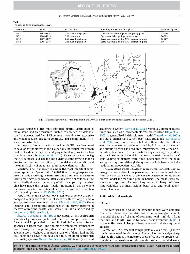
Fig. 1. Natural distribution of maritime pine in the world and limit of the ecoregions (coastal and interior) in Galicia.

Table 1The national forest inventories in Spain.

Inventory Years Stratification Sampling method and field plots Number of plots

NFI1 1965–1974 Grid over photographs Optimal allocation of plots; temporary plots 65,000NFI2 1986–1995 Grid over maps Systematic 1-km grid; permanent plots 84,203NFI3 1997–2007 Grid over digital maps Same systematic grid as NFI2; permanent plots 95,327NFI4 2008–2018 Grid over digital maps Same systematic grid as NFI2; permanent plots NA

J.G. Álvarez-González et al. / Forest Ecology and Management xxx (2013) xxx–xxx 3

database represents the most complete spatial distribution ofmany stand and tree variables. Such a comprehensive databasecould not be obtained from PPN because it would be too expensiveand would require long-term continuity and commitment in re-search infrastructure.

In the past, observations from the Spanish NFI have been usedto develop forest growth models, especially individual tree growthmodels, for different species and geographical regions, (refer to acomplete review by Bravo et al., 2012). These approaches, usingthe NFI database, did not include dynamic stand growth modelsdue to two reasons: the difficulty to model stand mortality andthe unavailability of stand age as an independent variable.

Maritime pine (P. pinaster) is among the most important conif-erous species in Spain, with 1,680,000 ha of single-species ormixed stands occurring in both artificial plantations and naturalforests that have regenerated after clear-cutting or wildfires. Thewide distribution and the variety of sites occupied by maritimepine have made this species highly important in Galicia wherethe forest industry has potential access to more than 39 millionm3 of standing timber (MMAMRM, 2011).

Populations of this species show a high level of genetic and phe-notypic diversity due to the use of seeds of different origins and togenotype–environment interactions (Alía et al., 1995, 1997). Thesefeatures lead to significant differences in the growth patterns inthe two ecoregions (coastal and interior) in Galicia, as defined byVega et al. (1993); see Fig. 1.

Álvarez González et al. (1999) developed a first ecoregionalstand-level growth and yield model for maritime pine stands inGalicia which provided rather limited information. Recentadvances in forest modelling and more detailed requirements byforest management regarding stand structure and different man-agement scenarios, have prompted a revision of that initial model.Two submodels have been developed to date: (i) an ecoregionalsite quality system (Álvarez González et al., 2005) and (ii) a basal


area growth system (Barrio et al., 2006). Moreover, different outputfunctions, such as a merchantable volume equation (Rojo et al.,2005), a generalised height-diameter model (Castedo et al., 2005)and stand biomass and carbon pool static equations (Barrio-Antaet al., 2006) were subsequently linked to these submodels. How-ever, the whole-stand model obtained by linking the submodelsand output functions still required improvement. Firstly, the origi-nal site index models were estimated using a base-age dependentapproach. Secondly, the models used to estimate the growth rate ofstem volume or biomass were fitted independently of the basalarea growth system, although the systems include basal area indi-rectly as an independent variable.

The aim of this article is to describe an example of establishing alinkage between data from permanent plot networks and datafrom the NFI to develop a biologically-consistent whole-standgrowth model for maritime pine in Galicia. The model uses thestate-space approach for modelling rates of change of threestate-variables: dominant height, basal area and total above-ground biomass.

2. Materials and methods

2.1. Data

The data used to develop the dynamic model were obtainedfrom two different sources: data from a permanent plot networkto model the rate of change of dominant height and data fromthe third and fourth Spanish National Forest Inventory (Table 1)to model the rates of change of basal area and total above-groundbiomass.

A total of 102 permanent sample plots of even-aged P. pinasterstands were used in this study. These plots were subjectivelyselected throughout the inventory areas of Galicia to provide rep-resentative information of site quality, age and stand density.




Two dominant trees were destructively sampled at each location(106 and 98 in the coastal and interior ecoregion, respectively).The trees were sectioned at the stump, at breast height, at 2.0 m,and then at 1-m intervals. The age at each section height wasdetermined in the laboratory. As cross-section lengths do not coin-cide with periodic height growth, height values at 2 year-incre-ments were estimated using the method of Carmean (1972) withthe modification proposed by Newberry (1991) for the topmostsection of the tree. A comparative study between six methods ofheight data correction in stem analysis showed that the Carmeanalgorithm provided the best performance (Dyer and Bailey, 1987).

Data from the III and IV Spanish National Forest Inventory havebeen used to estimate the rates of change of basal area and totalbiomass of the stands.

The number of stems per hectare (N), basal area (G) and domi-nant height (H, defined as the mean height of the 100 thickest treesper hectare) were calculated from the tree variable measurements,by using appropriate tree expansion factors as the Spanish NationalForest Inventory design of the field plot is based on concentricsubplots where the selection on sampled trees depends on theirdiameter. The expansion factor can be defined as the relationshipbetween the reference area (1 ha) and the subplots area adjustingthe values of the number of sampled trees to a per hectare value.

The values of the total above-ground biomass (Wtotal) were esti-mated using the compatible systems of tree biomass equationsdeveloped for maritime pine in Galicia (Diéguez-Aranda et al.,2009).

Sample plots in which dead or broadleaved trees accounted formore than 10% of basal area were rejected. An exhaustive examina-tion of the data was carried out to reject sample plots with changesin the species and reduction in dominant height or in basal area be-tween measurements. The number of sample plots used was 383(219 and 164 in the coastal and interior ecoregions, respectively).

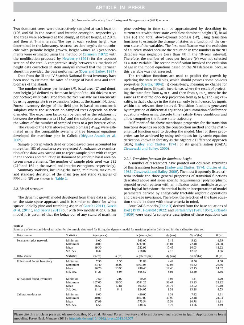
Summary statistics, including the mean, minimum, maximum,and standard deviation of the main tree and stand variables ofPPN and NFI are shown in Table 2.

2.2. Model structure

The dynamic growth model developed from these data is basedon the state-space approach and it is similar to those for whitespruce, loblolly pine and trembling aspen of García (2011), Garciaet al. (2011), and García (2013) but with two modifications. In thismodel it is assumed that the behaviour of any stand of maritime

Table 2Summary of some stand-level variables for the sample data used for fitting the dynamic m

Data source Statistics Age (years)

Permanent plot network Minimum 8.00Maximum 50.00Mean 19.30Std. dev. 8.47

Data source Statistics d (cm) h (m)

III National Forest Inventory Minimum 7.50 1.50Maximum 83.40 38.00Mean 26.76 13.90Std. dev. 11.23 5.94

IV National forest inventory Minimum 7.50 2.00Maximum 107.00 39.30Mean 26.57 17.81Std. dev. 11.12 6.11

Calibration data set Minimum 8.00Maximum 40.00Mean 17.99Std. dev. 6.58


pine evolving in time can be approximated by describing itscurrent state with three state variables: dominant height (H), basalarea (G) and total above-ground biomass (W), using transitionfunctions to estimate the change of states as a function of the cur-rent state of the variables. The first modification was the exclusionof a survival model because the reduction in tree number in the NFIdatabase was negligible (less than 4% in the 10-year interval).Therefore, the number of trees per hectare (N) was not selectedas a state variable. The second modification involved the exclusionof age in the model equations based on the NFI database, becausethis variable was not assessed.

The transition functions are used to predict the growth byupdating the state variables, which should possess some obviousproperties (García, 1994): (i) consistency, meaning no change forzero elapsed time; (ii) path-invariance, where the result of project-ing the state first from t0 to t1, and then from t1 to t2, must be thesame as that of the one-step projection from t0 to t2; and (iii) cau-sality, in that a change in the state can only be influenced by inputswithin the relevant time interval. Transition functions generatedby integration of differential equations (or summation of differenceequations when using discrete time) satisfy these conditions andallow computing the future state trajectory.

Fulfilment of the above mentioned properties for the transitionfunctions depends on both the construction method and the math-ematical function used to develop the model. Most of these prop-erties can be achieved by using techniques for dynamic equationderivation known in forestry as the Algebraic Difference Approach(ADA; Bailey and Clutter, 1974) or its generalisation (GADA;Cieszewski and Bailey, 2000).

2.2.1. Transition function for dominant heightA number of researchers have pointed out desirable attributes

of this transition function (Bailey and Clutter, 1974; Clutter et al.,1983; Cieszewski and Bailey, 2000). The most frequently listed cri-teria include the three general properties of transition functionsdescribed above and some specific requirements: polymorphism;sigmoid growth pattern with an inflexion point; multiple asymp-tote; logical behaviour; theoretical basis or interpretation of modelparameters derived by analytically tractable algebraic operationsand base-age invariance. Therefore, the selection of the base equa-tion should be done with these criteria in mind.

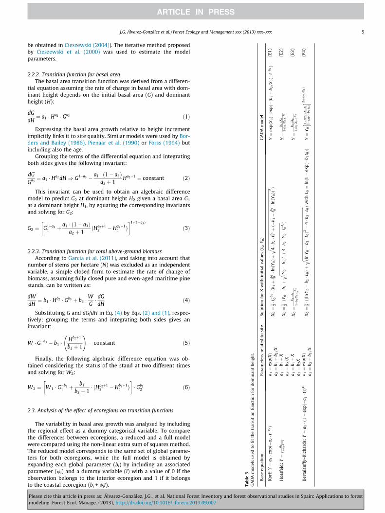
Four GADA models (Table 3) derived from the base equations ofKorf (1939), Hossfeld (1822) and Bertalanffy (1949, 1957), Richards(1959) were used (a complete description of these equations can

odel for maritime pine in Galicia and for the calibration data set.

N (stems/ha) dg (cm) G (m2/ha) H (m)

363.00 5.16 5.12 4.553237.00 35.01 72.48 24.581522.96 17.45 30.03 12.22

718.07 7.18 12.92 4.56

N (stems/ha) dg (cm) G (m2/ha) H (m)

31.83 4.49 0.56 4.005903.05 42.05 65.52 26.66

936.46 17.46 22.15 14.62865.57 8.01 12.59 5.66

19.24 9.95 1.41 8.295581.25 53.47 83.83 28.82

893.53 25.73 32.02 19.10824.05 8.31 13.88 4.53

430.00 6.31 7.42 5.913867.00 33.90 72.48 24.031773.54 15.54 30.78 11.11

638.37 5.73 13.76 3.49



GA

DA

mod

elffiffiffiffiffiffiffiffi

ffiffiffiffiffiffiffiffiffiffiffiffiffiffiffi

ffiffiffiffiffiffiffiffiffiffiffiffiffiffiffiffi


b 3 oþð�

b 1�

tb 3 0�l

nðY

0ÞÞ

2Þ

Y¼

expð

X0Þ�

expð�ðb

1þ

b 2=

X0Þ�

t�b 3Þ

(E1)


0�t�

b 3oÞ

Y¼

b 1þ

X0

1þb 2=

X0�t�

b 3(E

2)

Y¼

b 1þ

X0

1þb 2�X

0�t�

b 3(E

3)

ffiffiffiffiffiffiffiffiffiffiffiffiffiffiffiffiffiffiffiffiffiffiffi

ffiffiffiffiffiffiffiffiffiffi

0Þ2�

4�b

3�L

0Þ

wit

hL 0¼

ln½1�

expð�

b 1t 0Þ�

Y¼

Y0

1�ex

pð�

b 1�tÞ

1�ex

pð�

b 1�t 0Þ

hi ðb 2

þb 3=

X0Þ

(E4)


be obtained in Cieszewski (2004)). The iterative method proposedby Cieszewski et al. (2000) was used to estimate the modelparameters.

2.2.2. Transition function for basal areaThe basal area transition function was derived from a differen-

tial equation assuming the rate of change in basal area with dom-inant height depends on the initial basal area (G) and dominantheight (H):

dGdH¼ a1 � Ha2 � Ga3 ð1Þ

Expressing the basal area growth relative to height incrementimplicitly links it to site quality. Similar models were used by Bor-ders and Bailey (1986), Pienaar et al. (1990) or Forss (1994) butincluding also the age.

Grouping the terms of the differential equation and integratingboth sides gives the following invariant:

dGGa3¼ a1 � Ha2 dH) G1�a3 � a1 � ð1� a3Þ

a2 þ 1Ha2þ1 ¼ constant ð2Þ

This invariant can be used to obtain an algebraic differencemodel to predict G2 at dominant height H2 given a basal area G1

at a dominant height H1, by equating the corresponding invariantsand solving for G2:

G2 ¼ G1�a31 þ a1 � ð1� a3Þ

a2 þ 1ðHa2þ1

2 � Ha2þ11 Þ

� �1=ð1�a3Þ

ð3Þ

for

dom

inan

the

ight

.

Para

met

ers

rela

ted

tosi

teSo

luti

onfo

rX

wit

hin

itia

lva

lues

(t0,Y

0)

a 1¼

expðXÞ

X0¼

1 2�t�

b 30�ð

b 1þ

tb3 0�l

nðY

0Þþ

ffiffiffiffiffiffiffiffiffiffiffiffiffiffiffi

4�b

2�t

qa 2¼

b 1þ

b 2=

Xa 1¼

b 1þ

XX

0¼

1 2�ð

Y0�

b 1þ



ffiffiffiffiffiffiffiffiffiffiffiffi

ðY0�

b 1Þ2þ

4�b

2�Y

qa 2¼

b 2=X

a 1¼

b 1þ

XX

0¼

Y0�

b 11�

b 2�Y

0�t�

b 3o

a 2¼

b 2X

�tÞÞ

a 3a 1¼

expðXÞ

X0¼

1 2�ððln

Y0�

b 2�L

0Þþ


ffiffiffiffiffiffiffiffiffiffiffiffi

ðlnY

0�

b 2�L

qa 3¼

b 2þ

b 3=

X

2.2.3. Transition function for total above-ground biomassAccording to Garcia et al. (2011), and taking into account that

number of stems per hectare (N) was excluded as an independentvariable, a simple closed-form to estimate the rate of change ofbiomass, assuming fully closed pure and even-aged maritime pinestands, can be written as:

dWdH¼ b1 � Hb2 � Gb3 þ b3 �

WG� dGdH

ð4Þ

Substituting G and dG/dH in Eq. (4) by Eqs. (2) and (1), respec-tively; grouping the terms and integrating both sides gives aninvariant:

W � G�b3 � b1 �Hb2þ1

b2 þ 1

!¼ constant ð5Þ

Finally, the following algebraic difference equation was ob-tained considering the status of the stand at two different timesand solving for W2:

W2 ¼ W1 � G�b31 þ b1

b2 þ 1� ðHb2þ1

2 � Hb2þ11 Þ

� �� Gb3

2 ð6Þ

Tabl

e3

GA

DA

mod

els

used

tofi

tth

etr

ansi

tion

func

tion

Bas

eeq

uat

ion

Kor

f:Y¼

a 1�e

xpð�

a 2�t�

a 3Þ

Hos

sfel

d:Y¼

a 11þ

a 2�t�

a 3

Ber

tala

nff

y–R

ich

ards

:Y¼

a 1�ð

1�

expð�

a 2

2.3. Analysis of the effect of ecoregions on transition functions

The variability in basal area growth was analysed by includingthe regional effect as a dummy categorical variable. To comparethe differences between ecoregions, a reduced and a full modelwere compared using the non-linear extra sum of squares method.The reduced model corresponds to the same set of global parame-ters for both ecoregions, while the full model is obtained byexpanding each global parameter (bi) by including an associatedparameter (/i) and a dummy variable (I) with a value of 0 if theobservation belongs to the interior ecoregion and 1 if it belongsto the coastal ecoregion (bi + /iI).

Please cite this article in press as: Álvarez-González, J.G., et al. National Forest Inventory and forest observational studies in Spain: Applications to forestmodeling. Forest Ecol. Manage. (2013), http://dx.doi.org/10.1016/j.foreco.2013.09.007



2.4. Parameter estimation and model selection

The state-space approach has been widely used to developstand growth models and usually each transition function is fittedseparately. However, there exists a cross dependency of dominantheight and basal area because they are independent variables in anequation and dependent variables in, at least, one other equation.This cross-dependency may be the cause for errors by violatingthe assumption of independence. Due to the different structureof the two databases used, the transition function for dominantheight was fitted separately and the other two transition functionswere fitted simultaneously to remove simultaneous equation biasusing the full information maximum likelihood (FIML).

In the general formulation of the dynamic equations, theerror terms eij are assumed to be independent and identicallydistributed with zero mean. Nevertheless, because of thelongitudinal nature of the data sets used for model fitting,correlations between the residuals within the same plot maybe expected. To overcome any possible autocorrelation, the errorwas modelled using a continuous autoregressive error structure(CAR(x)), which accounted for the time between measurements.Estimation of the parameters was carried out with the MODELprocedure of SAS/ETS� (SAS Institute Inc., 2004). The CAR(x) er-ror structure was programmed in this procedure which allowsfor dynamic updating of the residuals.

The comparison of the estimates for the different models wasbased on numerical and graphical analyses of the residuals. Twostatistical criteria were examined: adjusted model efficiency(MEadj) and Root Mean Square Error (RMSE). The expressions ofthese statistics are summarised as follows:

ME ¼Pn

i¼1ðyi � yiÞ2=ðn� pÞPni¼1ðyi � �yÞ2=ðn� 1Þ

ð7Þ

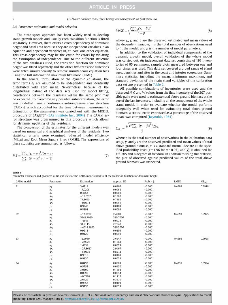
Table 4Parameter estimates and goodness-of-fit statistics for the GADA models used to fit the tra

GADA model Parameter Estimation A

E1 b1 3.4718 0.b2 17.0208 0.b3 0.4354 0.U1 �15.0765 0.U2 73.8695 0.U3 �0.0573 0.q1 0.9245 0.q2 0.8891 0.

E2 b1 �12.3232 2.b2 5348.7020 32b3 1.4848 0.U1 31.2115 2.U2 �4018.1600 34q1 0.9613 0.q2 0.9129 0.

E3 b1 72.6939 2.b2 �2.9928 0.b3 1.4858 0.U1 �27.8617 2.U2 �5.0838 0.q1 0.9615 0.q2 0.9130 0.

E4 b1 0.0493 0.b2 0.5758 0.b3 3.0500 0.U1 0.0099 0.U2 �0.7797 0.U3 2.6729 0.q1 0.9654 0.q2 0.9135 0.


RMSE ¼

ffiffiffiffiffiffiffiffiffiffiffiffiffiffiffiffiffiffiffiffiffiffiffiffiffiffiffiffiffiffiffiPni¼1ðYi � Y iÞ

2

n� p

sð8Þ

where yi, yi and �y are the observed, estimated and mean values ofthe dependent variable, n is the total number of observations usedto fit the model, and p is the number of model parameters.

In addition to the validation of individual components of thedynamic growth model, overall validation of the whole modelwas carried out. An independent data set consisting of 191 inven-tories of 65 permanent sample plots measured between one andfour times was used. This data set covered a broad range of standages, densities and sites in the coast and interior ecoregions. Sum-mary statistics, including the mean, minimum, maximum, andstandard deviation of the main stand variables of the calibrationdata set are presented in Table 2.

All possible combinations of inventories were used and theobserved H, G and W values from the first inventory of the 207 pos-sible pairs were used to estimate total above ground biomass at theage of the last inventory, including all the components of the wholestand model. In order to evaluate whether the model performsacceptably well when used for estimating total above-groundbiomass, a critical error, expressed as a percentage of the observedmean, was computed (Reynolds, 1984):

Ecrit: ¼

ffiffiffiffiffiffiffiffiffiffiffiffiffiffiffiffiffiffiffiffiffiffiffiffiffiffiffiffiffiffiffiffiffiffiffis2Pn

i¼1ðyi � yiÞ2q

=v2crit:

�yð9Þ

where n is the total number of observations in the calibration dataset, yi, yi and �y are the observed, predicted and mean values of totalabove-ground biomass, s is a standard normal deviate at the spec-ified probability level (s = 1.96 for a = 0.05), and v2

n is obtained fora = 0.05 and n degrees of freedom. In addition to using this statistic,the plot of observed against predicted values of the total aboveground biomass was inspected.

nsition function for dominant height.

pprox. SE Prob. > |t| RMSE MEadj

0266 <0.0001 0.4903 0.99180964 <0.00010069 <0.00011380 <0.00017386 <0.00010051 <0.00010108 <0.00010063 <0.0001

4808 <0.0001 0.4693 0.99250.7000 <0.0001

0073 <0.00017948 <0.00016.2000 <0.0001

0103 <0.00010059 <0.0001

6647 <0.0001 0.4694 0.99251863 <0.00010073 <0.00019467 <0.00018212 <0.00010108 <0.00010059 <0.0001

0008 <0.0001 0.4731 0.99240450 <0.00011453 <0.00010014 <0.00011117 <0.00013670 <0.00010103 <0.00010059 <0.0001



02468

10121416182022242628303234

0 5 10 15 20 25 30 35 40 45 50 55 0 5 10 15 20 25 30 35 40 45 50 55Age (years)

Dom

inan

t hei

ght (

m)

02468

10121416182022242628303234

Age (years)

Dom

inan

t hei

ght (

m)

02468

10121416182022242628303234

Age (years)

Dom

inan

t hei

ght (

m)

02468

10121416182022242628303234

Age (years)

Dom

inan

t hei

ght (

m)

02468

10121416182022242628303234

Age (years)

Dom

inan

t hei

ght (

m)

02468

10121416182022242628303234

Age (years)

Dom

inan

t hei

ght (

m)

02468

10121416182022242628303234

Age (years)

Dom

inan

t hei

ght (

m)

02468

10121416182022242628303234

Age (years)

Dom

inan

t hei

ght (

m)

0 5 10 15 20 25 30 35 40 45 50 55

0 5 10 15 20 25 30 35 40 45 50 550 5 10 15 20 25 30 35 40 45 50 55

0 5 10 15 20 25 30 35 40 45 50 55

0 5 10 15 20 25 30 35 40 45 50 55 0 5 10 15 20 25 30 35 40 45 50 55

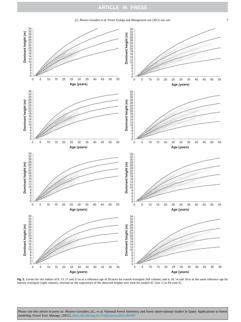
Fig. 2. Curves for site indices of 9, 13, 17 and 21 m at a reference age of 20 years for coastal ecoregion (left column) and 6, 10, 14 and 18 m at the same reference age forinterior ecoregion (right column), overlaid on the trajectories of the observed heights over time for models E1 (row 1) to E4 (row 4).


Please cite this article in press as: Álvarez-González, J.G., et al. National Forest Inventory and forest observational studies in Spain: Applications to forestmodeling. Forest Ecol. Manage. (2013), http://dx.doi.org/10.1016/j.foreco.2013.09.007



3. Results and discussion

3.1. Transition function for dominant height

Models E1–E4 were first fitted using nonlinear least squareswithout expanding the error terms to account for autocorrelation.A trend in residuals as a function of age lag residuals within thesame tree was evident in all the equations and was corrected usinga CAR(2) error structure. From a practical point of view, the auto-correlation parameters are generally ignored when using the sitemodel for predicting height and site index. The main purpose inusing that particular autocorrelation error structure was to obtainconsistent estimates of the parameters and their standard errors.

02468

10121416182022242628303234

Age (years)

Dom

inan

t hei

ght (

m)

0 5 10 15 20 25 30 35 40 45 50 55

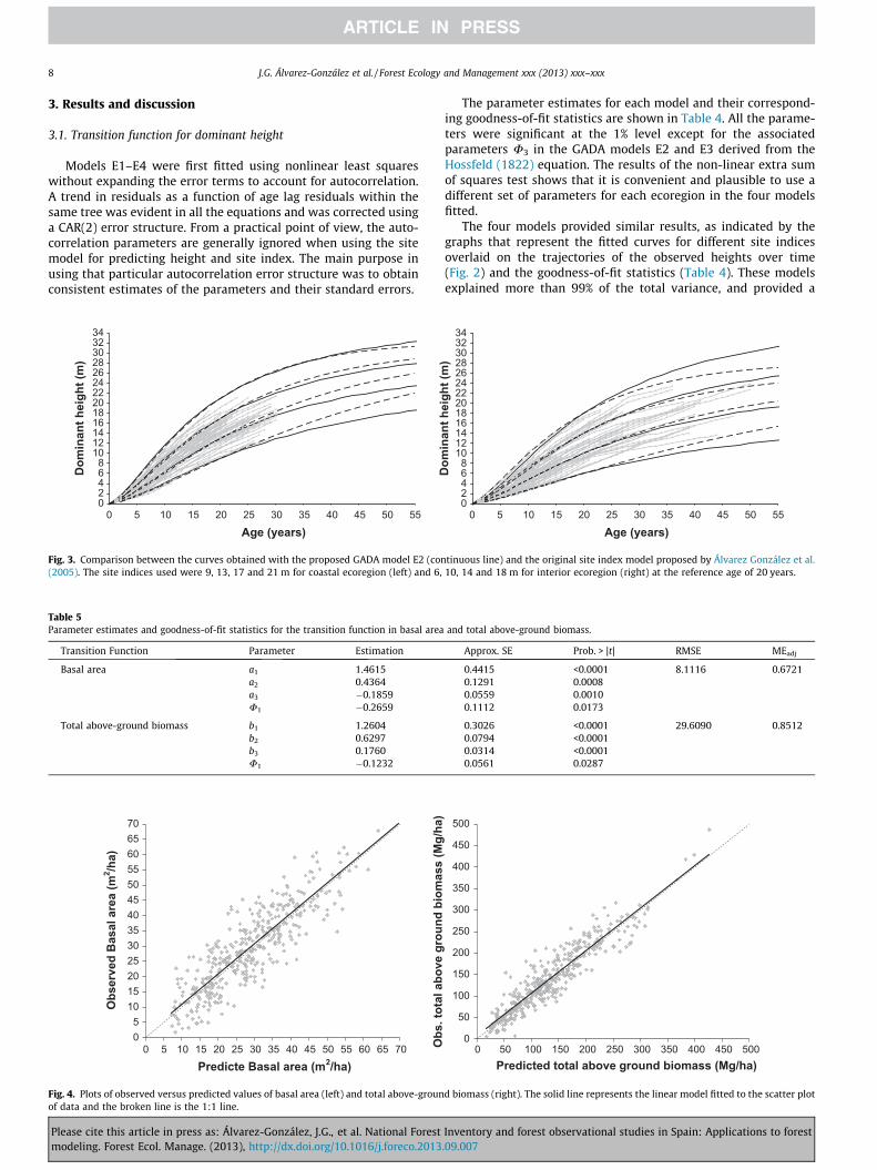
Fig. 3. Comparison between the curves obtained with the proposed GADA model E2 (con(2005). The site indices used were 9, 13, 17 and 21 m for coastal ecoregion (left) and 6,

Table 5Parameter estimates and goodness-of-fit statistics for the transition function in basal area

Transition Function Parameter Estimation

Basal area a1 1.4615a2 0.4364a3 �0.1859U1 �0.2659

Total above-ground biomass b1 1.2604b2 0.6297b3 0.1760U1 �0.1232

05

10152025303540455055606570

0 5 10 15 20 25 30 35 40 45 50 55 60 65 70

Predicte Basal area (m2/ha)

Obs

erve

d B

asal

are

a (m

2 /ha)

Fig. 4. Plots of observed versus predicted values of basal area (left) and total above-grounof data and the broken line is the 1:1 line.


The parameter estimates for each model and their correspond-ing goodness-of-fit statistics are shown in Table 4. All the parame-ters were significant at the 1% level except for the associatedparameters U3 in the GADA models E2 and E3 derived from theHossfeld (1822) equation. The results of the non-linear extra sumof squares test shows that it is convenient and plausible to use adifferent set of parameters for each ecoregion in the four modelsfitted.

The four models provided similar results, as indicated by thegraphs that represent the fitted curves for different site indicesoverlaid on the trajectories of the observed heights over time(Fig. 2) and the goodness-of-fit statistics (Table 4). These modelsexplained more than 99% of the total variance, and provided a

02468

10121416182022242628303234

0 5 10 15 20 25 30 35 40 45 50 55

Age (years)

Dom

inan

t hei

ght (

m)

tinuous line) and the original site index model proposed by Álvarez González et al.10, 14 and 18 m for interior ecoregion (right) at the reference age of 20 years.

and total above-ground biomass.

Approx. SE Prob. > |t| RMSE MEadj

0.4415 <0.0001 8.1116 0.67210.1291 0.00080.0559 0.00100.1112 0.0173

0.3026 <0.0001 29.6090 0.85120.0794 <0.00010.0314 <0.00010.0561 0.0287

0

50

100

150

200

250

300

350

400

450

500

0 50 100 150 200 250 300 350 400 450 500Predicted total above ground biomass (Mg/ha)

Obs

. tot

al a

bove

gro

und

biom

ass

(Mg/

ha)

d biomass (right). The solid line represents the linear model fitted to the scatter plot




random pattern of residuals around zero with homogeneousvariance and no detectable significant trends.

Selection of the model was thus based on visual inspection ofthe graphs shown in Fig. 2 and the values of the asymptotes. ModelE4 derived from the Bertalanffy–Richards base equation, andmodel E1 derived from the Korf base equation, showed higherasymptotes for the best sites. These asymptotes seem unrealisticfor this species, especially for model E1. Models E2 and E3, derivedfrom the Hossfeld base equation, are very similar; however, a slightreduction in dominant height growth for old ages in the best sitescan be inferred for model E3. Thus, from the four dynamicequations finally evaluated for height growth prediction and siteclassification of maritime pine stands in Galicia, model E2, i.e.the GADA formulation derived from the Hossfeld (1822) modelby considering parameters a1 and a2 as related to site productivity,was finally selected:

H ¼ ð�12:3232þ 31:2115 � IÞ þ X0

1þ ð5348:702� 4018:160 � IÞ=X0 � t�1:4848 ; with ð10Þ

X0 ¼12� H0 � ð�12:3232þ 31:2115 � IÞ þ

ffiffiffiffiffiffiffiffiffiffiffiffiffiffiffiffiffiffiffiffiffiffiffiffiffiffiffiffiffiffiffiffiffiffiffiffiffiffiffiffiffiffiffiffiffiffiffiffiffiffiffiffiffiffiffiffiffiffiffiffiffiffiffiffiffiffiffiffiffiffiffiffiffiffiffiffiffiffiffiffiffiffiffiffiffiffiffiffiffiffiffiffiffiffiffiffiffiffiffiffiffiffiffiffiffiffiffiffiffiffiffiffiffiffiffiffiffiffiffiffiffiffiffiffiffiffiffiffiffiffiffiffiffiffiffiffiffiffiffiffiffiffiffiffiffiffiffiffiffiffiffiffiffiffiffiffiffiffiffiffiffiffiffiffiffiðH0 � ð�12:3232þ 31:2115 � IÞÞ2 þ 4 � ð5348:702� 4018:16 � IÞ � H0 � t�1:4848

o

q� �ð11Þ

where H0 and t0 represent the predictor dominant height (m) andage (years), H is the predicted dominant height at age t and I is adummy variable with the value 1 for the coastal ecoregion and 0for the interior ecoregion. Eq. (9) explained 99.25% of the totalvariance of the data, and its Root Mean Square Error (RMSE) was0.4693 m. Fig. 3 shows the comparison between the GADAmodel finally selected and the original model proposed for thisspecies in Galicia by Álvarez González et al. (2005). For the coastalecoregion the curves showed a similar pattern during the first25 years and after that the new models seem to represent moreadequately the behaviour of the observed data, especially for poorquality sites. For the interior ecoregion, the original curves are anaccurate representation of the growth pattern of the stem analysisdata for young ages, however, the new curves are more realistic forthe overall growth pattern.

R2 = 0.9718

0

50

100

150

200

250

300

0 50 100 150 200 250 300Predicted total above ground biomass (Mg/ha)

Obs

. tot

al a

bove

gro

und

biom

ass

(Mg/

ha)

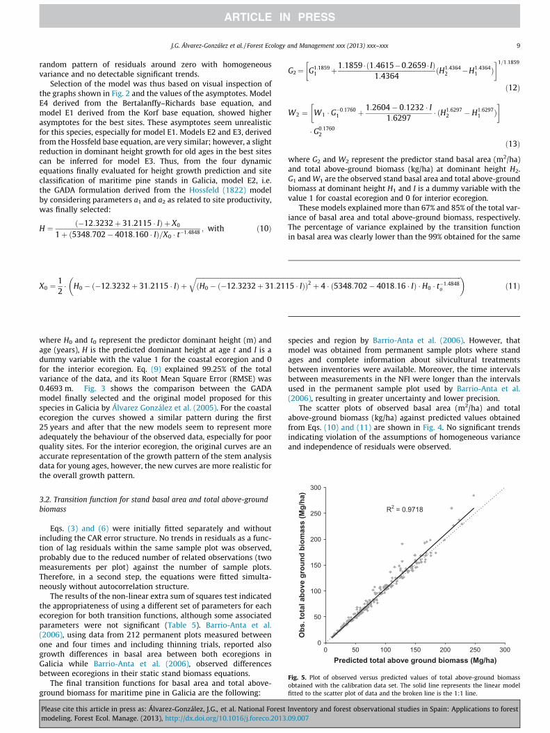
Fig. 5. Plot of observed versus predicted values of total above-ground biomassobtained with the calibration data set. The solid line represents the linear modelfitted to the scatter plot of data and the broken line is the 1:1 line.

3.2. Transition function for stand basal area and total above-groundbiomass

Eqs. (3) and (6) were initially fitted separately and withoutincluding the CAR error structure. No trends in residuals as a func-tion of lag residuals within the same sample plot was observed,probably due to the reduced number of related observations (twomeasurements per plot) against the number of sample plots.Therefore, in a second step, the equations were fitted simulta-neously without autocorrelation structure.

The results of the non-linear extra sum of squares test indicatedthe appropriateness of using a different set of parameters for eachecoregion for both transition functions, although some associatedparameters were not significant (Table 5). Barrio-Anta et al.(2006), using data from 212 permanent plots measured betweenone and four times and including thinning trials, reported alsogrowth differences in basal area between both ecoregions inGalicia while Barrio-Anta et al. (2006), observed differencesbetween ecoregions in their static stand biomass equations.

The final transition functions for basal area and total above-ground biomass for maritime pine in Galicia are the following:


G2¼ G1:18591 þ1:1859 � ð1:4615�0:2659 � IÞ

1:4364ðH1:4364

2 �H1:43641 Þ

� �1=1:1859

ð12Þ

W2 ¼ W1 � G�0:17601 þ 1:2604� 0:1232 � I

1:6297� ðH1:6297

2 � H1:62971 Þ

� �

� G0:17602

ð13Þ

where G2 and W2 represent the predictor stand basal area (m2/ha)and total above-ground biomass (kg/ha) at dominant height H2.G1 and W1 are the observed stand basal area and total above-groundbiomass at dominant height H1 and I is a dummy variable with thevalue 1 for coastal ecoregion and 0 for interior ecoregion.

These models explained more than 67% and 85% of the total var-iance of basal area and total above-ground biomass, respectively.The percentage of variance explained by the transition functionin basal area was clearly lower than the 99% obtained for the same

species and region by Barrio-Anta et al. (2006). However, thatmodel was obtained from permanent sample plots where standages and complete information about silvicultural treatmentsbetween inventories were available. Moreover, the time intervalsbetween measurements in the NFI were longer than the intervalsused in the permanent sample plot used by Barrio-Anta et al.(2006), resulting in greater uncertainty and lower precision.

The scatter plots of observed basal area (m2/ha) and totalabove-ground biomass (kg/ha) against predicted values obtainedfrom Eqs. (10) and (11) are shown in Fig. 4. No significant trendsindicating violation of the assumptions of homogeneous varianceand independence of residuals were observed.




A critical error of 19.4% was also obtained for total above-ground biomass. The critical error obtained with the proposedmodel is higher than the 15.3% obtained for projecting total standvolume in Scots pine in Galicia (Diéguez-Aranda et al., 2006) andthe 10.9%, 11.9% and 17.3% obtained for the same stand variablein radiata pine in Galicia, considering time intervals of 3, 6 and9 years, respectively (Castedo-Dorado et al., 2007). However, thosemodels included age as an independent variable. Age is a veryimportant variable in modelling even-aged stands and thereforethe differences in critical error were expected. Nevertheless,considering the required accuracy in forest growth modelling,where a mean prediction error of ±10–20% is generally acceptable(Huang et al., 2003), we can state that the dynamic model providessatisfactory estimates.

A plot of observed against predicted values of total above-ground biomass, estimated using the whole stand growth modelwith the calibration data set, is shown in Fig. 5. The linear modelfitted to the scatter plot behaved well (R2 = 0.9718), although thereappears to be a slight tendency towards underestimation.

4. Conclusions

Forest observational studies provide the essential informationfor modeling ecosystem structure and dynamics. In Spain, thereare important synergies between long-term observational plotsand the National Forest Inventory. A simple dynamic growth modelfor intensively managed even-aged stands is presented as anexample of how the data are converted into predictive tools forimproved ecosystem design. While the dynamic model presentedin this paper is specific to the Atlantic ecoregion of Spain, the ap-proaches used to develop the model have broad applicability forintensively managed forests. The model requires the current valuesof three stand variables: site index (or dominant height and age ofdominant trees), basal area and total above ground biomass toestimate the future values of these variables. The required standcharacteristics can be easily obtained by measuring all the diame-ters in a sample plot and at least a sub-sample of heights toestimate a local height-diameter relationship. The main restrictionof the models based on the NFI database is the long intervalbetween successive measurements, especially for fast-growingspecies. However, the complete database (I–IV NFI) covers a periodof 40 years and, since models based on the state-space approachcan be linked with other additional modules, such as climate,nutrition or carbon cycling modules (e.g. Garcia et al., 2011), hy-brid models could be developed using the NFI information. Suchhybrid models could take into account the responses to climatechange or could improve model performance when empiricalobservations are scarce.

The proposed stand growth modeling approach represents anew alternative for situations when stand age is not available.However, stand age is an important variable and it is recom-mended that in the future, data from permanent plot networks,including thinning trials, are combined with the NFI database totest and improve our approach.

All the equations proposed in this paper could be included in thedynamic growth and yield simulator GesMO� for single-species,even-aged stands. GesMO, which is available at http://www.usc.es/uxfs, enables users to simulate the various effects of differentsilvicultural treatments (depending on the type, intensity and ageof thinning, and the rotation age) including an economic evaluation.

Acknowledgements

This research was initiated during a research visit by JuanGabriel Álvarez-González to the Forestry ResearchCentre (INIA-CI-


FOR), with financial support from the ‘‘ProgramaNacional deMovilidad de Recursos Humanos de Investigación de2010’’ (REF:PR2010-0467. PN I+D+i 2008–2011).

References

Adame, P., del Rio, M., Cañellas, I., 2010. Ingrowth model for pyrenean oak stands innorth-western Spain using continuous forest inventory data. Eur. J. For. Res.129, 669–678.

Alberdi Asensio, I., Condés Ruiz, S., Martínez Millán, J., Martínez, Saura, de Toda, S.,Sánchez Peña, G., Pérez Martín, F., Villanueva Aranguren, J.A., Vallejo Bombin, R.,2010. Spanish national forest inventory. In: Tomppo, E., Gschwantner, T.,Lawrence, M., McRoberts, R.E. (Eds.), National Forest Inventories. Pathways forCommon Reporting. Springer, pp. 527–540.

Alía, R., Gil, L., Pardos, J.A., 1995. Performance of 43 Pinus pinaster provenances on 5locations in Central Spain. Silvae Genet. 44, 75–81.

Alía, R., Moro, J., Denis, J.B., 1997. Performance of Pinus pinaster Ait. provenances inSpain: interpretation of the genotype-environment interaction. Can. J. For. Res.27, 1548–1559.

Álvarez González, J.G., Rodríguez, R., Vega, G., 1999. Elaboración de un modelo decrecimiento dinámico para rodales regulares de Pinus pinaster Ait. en Galicia.Invest. Agr.: Sist. Rec. For. 8, 319–334.

Álvarez González, J.G., Ruiz, A.D., Rodríguez, R.J., Barrio, M., 2005. Development ofecoregion-based site index models for even-aged stands of Pinus pinaster Ait. inGalicia (north-western Spain). Ann. For. Sci. 62, 115–127.

Bailey, R.L., Clutter, J.L., 1974. Base-age invariant polymorphic site curves. For. Sci.20, 155–159.

Barrio Anta, M., Castedo Dorado, F., Diéguez-Aranda, U., Álvarez González, J.G.,Parresol, B.R., Rodríguez Soalleiro, R., 2006. Development of a basal area growthsystem for maritime pine in northwestern Spain using the generalized algebraicdifference approach. Can. J. For. Res 36, 1461–1474.

Barrio-Anta, M., Balboa-Murias, M.A., Castedo-Dorado, F., Diéguez-Aranda, U.,Álvarez-González, J.G., 2006. An ecoregional model for estimating volume,biomass and carbon pools in maritime pine stands in Galicia (northwesternSpain). For. Ecol. Manage. 223, 24–34.

Bertalanffy, L.V., 1949. Problems of organic growth. Nature 163, 156–158.Bertalanffy, L.V., 1957. Quantitative laws in metabolism and growth. Quart. Rev.

Biol. 32, 217–231.Borders, B.E., Bailey, R.L., 1986. A compatible system of growth and yield equations

for slash pine fitted with restricted three-stage least squares. For. Sci. 32, 185–201.

Bravo, F., Ordoñez, C., Lizarralde, I., Bravo-Oviedo, A., Guerra Burton, B., Del PesoTaranco, C., Domínguez Domínguez, M., Osorio Vélez, L.F., 2004. Red de parcelasy experimentos del grupo de investigación sobre gestión forestal sostenible dela ETS de ingenierías agrarias de Palencia (Universidad de Valladolid).Cuadernos SECF 18, 237–242.

Bravo, F., Álvarez-González, J.G., del Río, M., Barrio-Anta, M., Bonet, J.A., Bravo-Oviedo, A., Calama, R., Castedo-Dorado, F., Crecente-Campo, F., Condés, S.,Diéguez-Aranda, U., González-Martínez, S.C., Lizarralde, I., Nanos, N., Madrigal,A., Martínez-Millán, F.J., Montero, G., Ordóñez, C., Palahí, M., Piqué, M.,Rodríguez, F., Rodríguez-Soalleiro, R., Rojo, A., Ruiz-Peinado, R., Sánchez-González, M., Trasobares, A., Vázquez-Piqué, J., 2012. Growth and yieldmodels in Spain: historical overview, contemporary examples andperspectives. <http://www.usc.es/uxfs/Books>.

Burkhart, H.E., 2008. Modelling growth and yield for intensively managed forests. J.For. Sci. 24 (3), 119–124.

Carmean, W.H., 1972. Site index curves for upland oaks in the Central States. For.Sci. 18, 109–120.

Castedo, F., Barrio, M., Parresol, B.R., Álvarez González, J.G., 2005. A stochasticheight-diameter model for maritime pine ecoregions in Galicia (northwesternSpain). Ann. For. Sci. 62, 455–465.

Castedo-Dorado, F., Diéguez-Aranda, U., Álvarez-González, J.G., 2007. A growthmodel for Pinus radiata D. Don stands in north-western Spain. Ann. For. Sci. 64,453–465.

Cieszewski, C.J., 2004. GADA Derivation of Dynamic Site Equations withPolymorphism and Variable Asymptotes from Richards, Weibull, and otherExponential Functions. University of Georgia PMRC-TR 2004-5.

Cieszewski, C.J., Bailey, R.L., 2000. Generalized algebraic difference approach: theorybased derivation of dynamic site equations with polymorphism and variableasymptotes. For. Sci. 46, 116–126.

Cieszewski, C.J., Harrison, M., Martin, S.W., 2000. Practical Methods for EstimatingNon-biased Parameters in Self-referencing Growth and Yield Models. Universityof Georgia, PMRC-TR 2000-7.

Clutter, J.L., Fortson, J.C., Pienaar, L.V., Brister, H.G., Bailey, R.L., 1983. TimberManagement: A Quantitative Approach. John Wiley and Sons Inc., New York.

Curtis, R.O., Hyink, D.M., 1985. Data for growth and yield models. In: Van Hooser,D.D., Van Pelt, N. (comps). Proceedings – growth and yield and othermensurational tricks: a regional technical conference. Gen. Tech. Rep. INT-193. USDA, Forest Service, Intermountain Research Station, pp. 1–5.

Diéguez-Aranda, U., Castedo, F., Álvarez, J.G., Rojo, A., 2006. Dynamic growth modelfor Scots pine (Pinus sylvestris L.) plantations in Galicia (north-western Spain).Ecol. Model. 191, 225–242.

Diéguez-Aranda, U., Rojo Alboreca, A., Castedo-Dorado, F., Álvarez González, J.G.,Barrio-Anta, M., Crecente-Campo, F., González González, J.M., Pérez-Cruzado, C.,


http://www.usc.es/uxfs

http://www.usc.es/uxfs

http://refhub.elsevier.com/S0378-1127(13)00621-X/h0005








































http://www.usc.es/uxfs/Books





























Rodríguez Soalleiro, López-Sánchez, C.A., Balboa-Murias, M.A., Gorgoso Varela,J.J., Sánchez Rodríguez, F., 1993. Herramientas selvícolas para la gestión forestalsostenible en Galicia. Consellería do Medio Rural, Xunta de Galicia.

Dyer, M.E., Bailey, R.L., 1987. A test of six methods for estimating true heights fromstem analysis data. For. Sci. 33, 3–13.

Echeverría, I., 1942. Ensayo de tablas de producción del Pinus insignis en el norte deEspaña. Boletines del I.F.I.E. 22, Madrid.

Echeverría, I., De Pedro, S., 1948. El Pinus pinaster en Pontevedra. Su productividadnormal y aplicación a la celulosa industrial. Boletines del I.F.I.E. 38, Madrid.

Forss, E., 1994. Das Wachstum der Baumart Acacia mangium in Südkalimantan,Indonesien. Magister Diss.. Fac. of Forestry, University of Göttingen.

García, O., 1994. The state-space approach in growth modelling. Can. J. For. Res. 24,1894–1903.

García, O., 2011. A parsimonious dynamic stand model for interior spruce in BritishColumbia. For. Sci. 57 (4), 265–280.

García, O., 2013. Building a dynamic growth model for trembling aspen in WesternCanada without age data. Can. J. For. Res. 43 (3), 256–265.

Garcia, O., Burkhart, H.E., Amateis, R.L., 2011. A biologically-consistent stand growthmodel for loblolly pine in the Piedmont physiographic region, USA. For. Ecol.Manage. 262, 2035–2041.

Hossfeld, J.W., 1822. Mathematik für Forstmänner, Ökonomen und Cameralisten(Gotha, 4. Bd., S. 310).

Huang, S., Yang, Y., Wang, Y., 2003. A critical look at procedures for validatinggrowth and yield models. In: Amaro, A., Reed, D., Soares, P. (Eds.), ModellingForest Systems. CAB International, Wallingford, Oxford shire, UK, pp. 271–293.

Korf, V., 1939. Pfispevek k matematicke definici vzrustoveho zakona lesnichporostii. Lesnicka prace 18, 339–356.

MMAMRM, 2011. Cuarto Inventario Forestal Nacional. Galícia. Dirección General deMédio Natural y Política Forestal. Ministerio de medio Ambiente, Medio Rural yMarino.


Montero, G., Madrigal, G., Ruiz-Peinado, R., Bachiller, A., 2004. Red de parcelasexperimentales permanentes del CIFOR-INIA. Cuadernos SECF 18, 229–236.

Newberry, J.D., 1991. A note on Carmean’s estimate of height from stem analysisdata. For. Sci. 37, 368–369.

Pienaar, L.V., Page, H., Rheney, J.W., 1990. Yield prediction for mechanically site-prepared slash pine plantations. South J. Appl. For. 14, 104–109.

Rennolls, K., 1997. Data requirements for forest modelling. In: Amaro, A., Tomé, M.(Eds.), Empirical and process-based models for forest tree and stand growthsimulation. Edições Salamandra, Lisboa, pp. 11–22.

Reynolds Jr., M.R., 1984. Estimating the error in model predictions. For. Sci. 30, 454–469.

Richards, F.J., 1959. A flexible growth function for empirical use. J. Exp. Bot. 10, 290–300.

Rojo, A., Perales, X., Sánchez-Rodríguez, F., Álvarez-González, J.G., Gadow, K.V.,2005. Stem taper functions for maritime pine (Pinus pinaster Ait.) in Galicia(Northwestern Spain). Eur. J. For. Res. 124, 177–186.

SAS Institute Inc. 2004. SAS/ETS� 9.1 User’s Guide. SAS Institute Inc., Cary, NC.Torres Álvarez, E., Suárez, M.A., Vázquez Piqué, J., Calzado Carretero, J.A., 2004.

Dispositivo experimental para el estudio de la influencia de los factoresambientales y silvícolas sobre el crecimiento de alcornoque. Cuadernos SECF 18,261–268.

Trasobares, A., Pukkala, T., Miina, J., 2004. Growth and yield model for uneven-agedmixtures of Pinus sylvestris L. and Pinus nigra Arn. In Catalonia, north-east Spain.Ann. For. Sci. 61, 9–24.

Vanclay, J.K., 1994. Modelling Forest Growth and Yield. Applications to MixedTropical Forests. CAB International, Wallingford, UK.

Vega, P., Vega, G., González, M., Rodríguez, A., 1993. Mejora del Pinus pinaster Ait.en Galicia. In: Silva Pando, J. (Ed.) I Congreso Forestal Español, vol. 2, 1993, pp.129–134.




















































Documents

National Forest Inventory and forest observational studies in Spain: Applications to forest modeling