Embed Size (px)
Citation preview
1
NATIONAL SPATIAL CROP YIELD SIMULATION USING GIS-BASED CROP PRODUCTION MODEL
Satya Priya and Ryosuke SHIBASAKI Center for Spatial Information Science
University of Tokyo, 4-6-1 Komaba Meguro-ku, Tokyo 153-8505, JAPAN
Phone: +81-3-5452-6412; Fax: +81-3-5452-6414 Email: [email protected]; [email protected]
ABSTRACT Traditional decision support systems based on crop simulation models are normally site-specific. In policy formulation, however, spatial variability of crop production often need to be evaluated due to different soil conditions, weather conditions and agricultural practices within a target-region. To address the spatial variability, a spatial model “Spatial EPIC” was developed based on a crop simulation model EPIC (Erosion Productivity Impact Calculator). Since site-specific crop simulation models require point-based or fine resolution data, it is necessary to feed the fine resolution data at each grid-cell in order to “spatialize” crop simulation models. The authors proposed a method to generate fine resolution data from coarse resolution data which are usually available at regional or national level. In addition, since the original EPIC crop management practices are static in nature, a dynamic adaptation loop is added to evaluate the impacts of agricultural practice changes over temporal scale. Validation of the spatial EPIC was conducted at different spatial scales, i.e. National scale (approx. 50km cell-size) and regional scale (approx. 10km cell-size) in India. Results showed that at both resolutions level crop yield varied significantly as a function of seasonal climatic variation, soil water holding characteristics and applied crop management strategies. Also, the study successfully demonstrated model applicability in evaluating an impact of climate changes over major cereal crops productivity at national level taking spatial variability into account. Keywords: Crop simulation models, Geographic Information Systems (GIS), Agroecosystem, National analysis and planning, Crop productivity. 1. INTRODUCTION There is an emerging need to support policy formulation and decision-making in agriculture at very large geographic scales. Typical issues are climate change impact assessment and formulation of mitigating measures, water resource allocation in a river basin at sub-continental scale such as Yellow River and Ganges River, and environmental impact assessment of agriculture activities in such a large river basin. In order to develop a decision support system, biophysical processes and human interactions such as adaptive changes of agricultural practice have to be modelled. The model should simulate, for example, how the changes of environment such as climate change may influence crop yield and how the changes in cropping pattern, cultivation intensity and management practices may affect the environment over time. Spatial variability in the impacts and changes of the processes need special attention in the modeling process. When we focus major crop production, it would be appropriate to apply process-based crop simulation model for the purposes above. However, crop simulation models usually need site specific characteristics such as weather, physical and chemical parameters of soil, water management, and agronomic practices (Whistler, et., al, 1986, Penning de Vries et al., 1989) as input data. Applicability
2
of these models can be extended to much boarder spatial scales by combining them with a Geographic Information System (GIS). Several researchers have demonstrated or discussed the strength of this concept for agricultural management decision and planning at various spatial scales (Dent and Thorton, 1988; Hoongenboom et al., 1990; Hoogenboom and Thorton 1990; Thorton and Dent 1987; Throrton and Dent 1990). Thornton (1991) discussed the possibility of linking GIS with crop models on a farm and regional level. Curry et. al. (1990) studied the crop model to find possible effects of climate change on agricultural productivity at regional level. Hoongenboom and Thornton (1990) applied GIS to bean, maize and sorghum crop models to test potential of linked systems for agro-technology transfer in Guatemala. The crop model CERES-SORGHUM, using IBSNAT standard input/output data formats, was linked to GIS to assist decision making in estimating sorghum production in Indian semiarid tropics. Calixtte et al. (1992) developed an Agricultural and Environmental Geographic Information System (AEGIS), which combined DSSAT crop models with GIS to assess the impact of different agricultural practices of Puerto Rico. However, there is no attempt to apply process-based crop simulation models at scale of a very large country or sub-continental scale. Since many of models applied to climate impact assessment at continental to global scale estimate potential productivity, not actual productivity, using climate data, effects of mitigation measures such as adaptation of agricultural practices can not be evaluated. The objective of this paper is to develop a GIS-based crop model, which can predict crop yield, plant growth and nutrient/moisture dynamics under different agricultural practices at national to sub-continental scale. At first, we have to evaluate how much accuracy can be achieved by “extending” the idea of GIS/crop model integration to large geographical scale using coarse resolution data, which are usually available at such large scale. Technically, we have to devise a mechanism to “generate” fine resolution data from coarse resolution data to run the models, which were originally developed as a site-specific model. Moreover, since some of process-based crop models are static in the sense that they can not take dynamic changes of practices into account, we have to modify them to simulate the impacts of dynamically changing practices. Therefore, the paper introduces the “Spatial-EPIC” (an extension of original EPIC), a dynamic adaptive crop growth model on GIS platform. A two-tier, country and regional level simulations were conducted to evaluate the model performances in India as a case study area. Finally to demonstrate potential of the model application, national scale climate change impact over rice crop is estimated in this paper. 2. DEVELOPMENT OF “SPATIAL-EPIC” In process of the development of “Spatial-EPIC”, the authors went for an extensive literature review pertaining crop environment management field scale models because of the fact that such crop models are the outcome of decades not years. The aim of this research in terms of model development was to select the most appropriate field scale/point based model rather than to start from scratch, and to develop them on a GIS platform with proper modifications to give a new approach through spatial modelling. 2.1 Model Selection Proper model selection is one of the most important step in any modelling exercise, if the model is not being developed from very beginning. It was kept in mind that the selected model should provide agricultural managers with a powerful tool to assess simultaneously the affect of farm practices on crop production as well as on soil and water resources. Other model selection criteria included minimum data requirements to run the model, wide usage, and a reasonable accuracy in predictions. The following models were reviewed: (1) CREAMS and GLEAMS; (2) AGNPS; (3) ANSWERS; (4) SWRRB; (5) DSSAT and (6) EPIC. CREAMS and GLEAMS are field scale continuous models, they do not possess a robust crop growth model (Ramanarayam 1994). ANSWERS and AGNPS were
3
eliminated as they are watershed scale models simulating the effect of single rainfall events and are not suited for simulating the continuous nature of plant growth (Binger 1990). The data requirements for these models are extensive (where the use of GIS data are helpful) because of the distributed nature of modelling. Furthermore distributed models provide tools to advance one`s understanding of physical processes, but for management purposes, their usefulness is limited (Grayson 1992). SWRRB and EPIC are almost synonymous, except for the fact that SWRRB is a basin scale simulation model. EPIC (Williams, J. R. and Sharpley, A.N.,1989), has improved residue-handling capabilities over SWRRB, and better nutrient cycling. Also EPIC has the added advantage of accounting for wind erosion (Binger 1990). DSSAT, crop simulation models and similar computer decision have been developed for each crop management and other related processes (IBSNAT, 1989). The limitation with DSSAT is that it doesn’t provide one model to simulate many crops instead it has models for all specific crops. Also, earlier it was not public domain software (recently they have started to distribute their code to the licensed user only) where the other researcher may take up for its further development as we did in case of EPIC model after having its source code. Therefore, based on the literature reviewed and expert opinion gathered from model developers, EPIC was selected for further development under the defined framework of this study. Some additional model features that favored the selection of EPIC are (Dumesnil 1993): ➀ . EPIC is a continuous, field scale agricultural management/water quality model. ➁ . EPIC is broad-based in terms of its components to model major biophysical processes which include weather, hydrology, erosion, nutrients (nitrogen and phosphorus) cycling, pesticide fate, soil temperature, crop growth, tillage, plant environmental controls and economics. ➂ . The data required by EPIC are relatively minimal and was made available after deriving the concept of generators (weather generator and slope generator). ➃ The model provides parameter data files for major crops, soils, and tillage practices. ➄ EPIC is also equipped with a stochastic weather generator, and ➅ . EPIC is capable of simulating the long-term effects of cropping systems on soil erosion and productivity in specific environments.
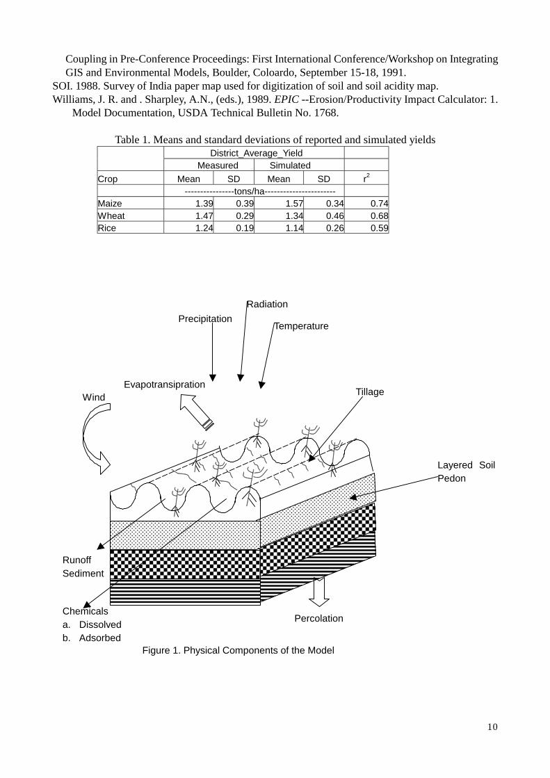
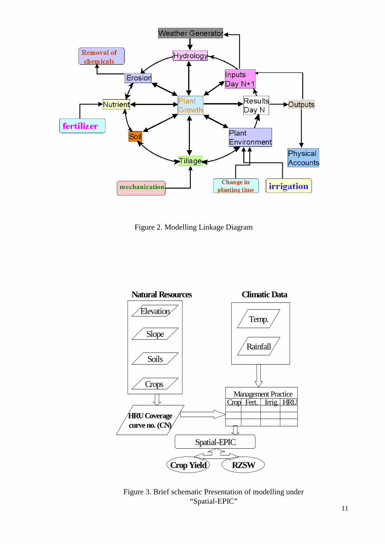
2.2 Biophysical Computation The model is composed of physically based components for simulating plant growth, nutrient, erosion, and related process for assessing crop productivity, determining optimal management strategies, erosion and so on. Simultaneously and realistically, model simulates all these physical processes. Commonly used input data are weather, crop, tillage, soil-attributes and management parameters. The model runs on defined rather derived cell size data layers provided by the user depending on their availability. Figure 1 shows physical factors considered in computing a mathematical model to find the effects of crop productivity coming from different processes. “Spatial-EPIC” is composed of physically based submodels for simulating weather, hydrology, erosion, plant nutrients, plant growth, soil tillage and management, and plant environment control. The model runs on daily time-step therefore, each model is linked subsequently and interactively with other sub models as demonstrated in figure 2. In brief, the computational procedures of all the submodels are described here under. Weather: daily rain, maximum and minimum temperature, solar radiation, wind and relative humidity can be given directly or else they can be generated stochastically. Hydrology: runoff, percolation, lateral subsurface flows are simulated. Erosion: it simulates soil erosion by wind and water (for this paper the erosion part has not been included). Nutrient Cycling: the model simulates, nitrogen and phosphorus fertilization, transformations, crop uptake and nutrient movement. Nutrient can be applied as mineral fertilizers, in irrigation water, or as animal manures. Soil: soil temperature responds to weather, soil water content and bulk density. It is computed daily in each soil layer. Tillage: the equipment used affects soil hydrology and nutrient cycling. The user can change the characteristics of simulated tillage equipment, if needed. Crop Growth: A single crop model capable of simulating major agronomic crops. Crop-specific parameters
4
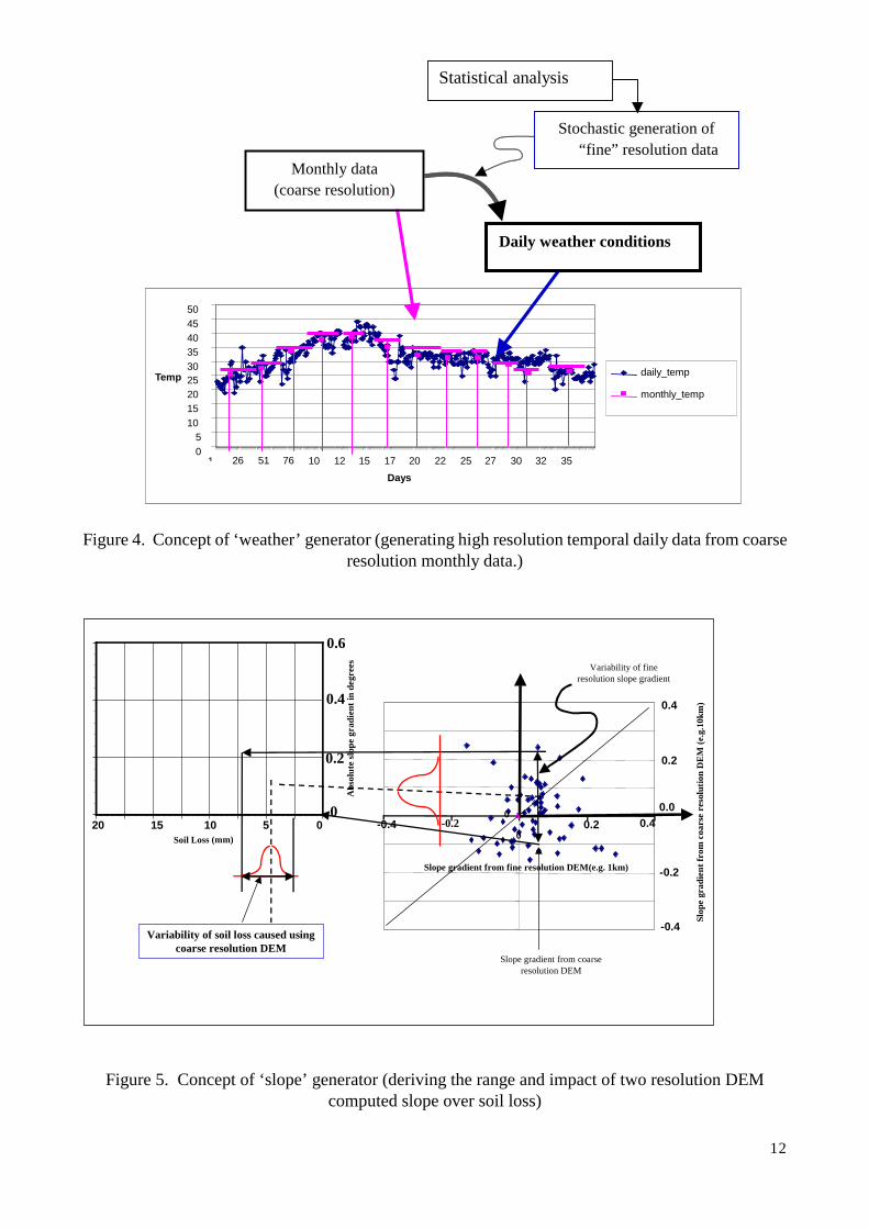
are available for most crops. The model also simulates crop grown in complete rotations. Plant Environment: It is capable of variety of cropping variables, management practices, and other naturally occurring processes. These include different crop characteristics, plant population, dates of planting and harvest, fertilization, irrigation, tillage and many more those are normally practiced in the field. Figure 3 shows a brief schematic presentation GIS data layers required for crop modelling and integrated model run process respectively under “Spatial-EPIC”. This serves as an example of listed natural resources and climatic data obtained from different sources and formats for creating GIS layers to feed the model inputs 2.3 Development of Dynamic Adaptations Loop The original EPIC is static with respect to management and technology. A single crop or rotation, tillage practice, conservation measure, crop planting and harvesting date, and machine sequence is specified prior to an EPIC simulation and cannot be varied during a simulation. The level of technology (such as plant genetic material and efficiency, plant varieties or cultivar, irrigation efficiencies, and so on) is also fixed. This was one of the main bottlenecks to apply EPIC for crop modelling over temporal scales because it can not adopt the management as per the climatic and resources prevailed. Therefore, the “Spatial-EPIC” carries a component where all these management and technologies practices have been made dynamic. With this, one can easily change the practices, crop rotation, other crop management like time-series fertilizer application, irrigation scheduling, tillage practice and so on as per the crop and area depending upon the resources and adaptations required. The management practices applied under this simulation were crop based as well as their respective growing seasons. Hence, the development of “Spatial-EPIC” with an addition of dynamic adaptations model is able to evaluate the impacts of agricultural practices more realistically over a temporal run which were lacking in the original EPIC model. 2.3 Generating “Fine” Resolution Data from “Coarse” Resolution Data As discussed before the “EPIC” model used for development is a field scale model. Hence the fine resolution data requirements was a big gap for applying it on a regional or national level scale, where only relatively coarse resolution data are usually available. The concept of “generators” helps fill the gap. The generators are used not to save data storage size but to provide high-resolution (temporal and spatial) data from coarse resolution data. The generators helped to integrate or establish the linkage of data to build a multi-scale GIS database. A weather generator model developed by Richardson (1981a) was used for generating the daily weather data from statistical characteristics of the actual recorded weather data. The model is designed to preserve the dependence in time, the internal correlation, and the seasonal characteristics that exist in actual daily weather data to compute their monthly coefficients. These coefficients were used to generate back the daily data for model input by stochastic simulation method for the said number of years as shown briefly in figure 4. The authors compared the estimated yield using recorded daily weather condition data vs. generated daily weather condition data, to see the differences, whereas after comparison they were negligibly small. By extending the idea underlying the weather generator to spatial dimension, the authors develop a slope generator, which generates fine resolution slope gradient from coarse resolution ones. Fine resolution slope gradient data is essential in estimating soil loss and resulting productivity degradation. Figure 5 illustrates the procedure of slope generation from 10 km resolution DEM data and how to apply the slope generator to soil loss estimation. The right part of the figure is a scatterogram of fine resolution slope gradient values (i.e. 1km grid size) against coarse resolution slope gradient values (i.e. 10km grid size). When a coarse resolution slope gradient value is given at a specific location, it can be inferred from the scatterogram to how much extent fine resolution slope gradient value can fluctuate at the same location. The range of fluctuation or the distribution of fine
5
resolution slope gradient can be converted to the distribution of soil loss through soil loss vs. absolute slope gradient curve in the left part of Figure 5. By integrating the distribution of soil loss, total soil loss can be estimated within a coarse grid cell from coarse resolution slope gradient. Unfortunately, due to the lack of appropriate validation data, soil loss estimation using the slope generator was not validated. The same kind of the idea, however, can be applied to generate a variety of spatial data such as soil data. Thus, dynamic linkage between short-term, fine scale data with relatively long-term and coarser resolution data can be established by devising nesting of observations at multiple spatio-temporal scales. 3. STUDY AREA AND DATASET
The chosen study area is India, lies to the north of equator, between 8°4’ and 37°6’ North and 68°7’ and
97°25’ East. It is bounded in the south by the Indian Ocean, in the west by the Arabian Sea, in the east by
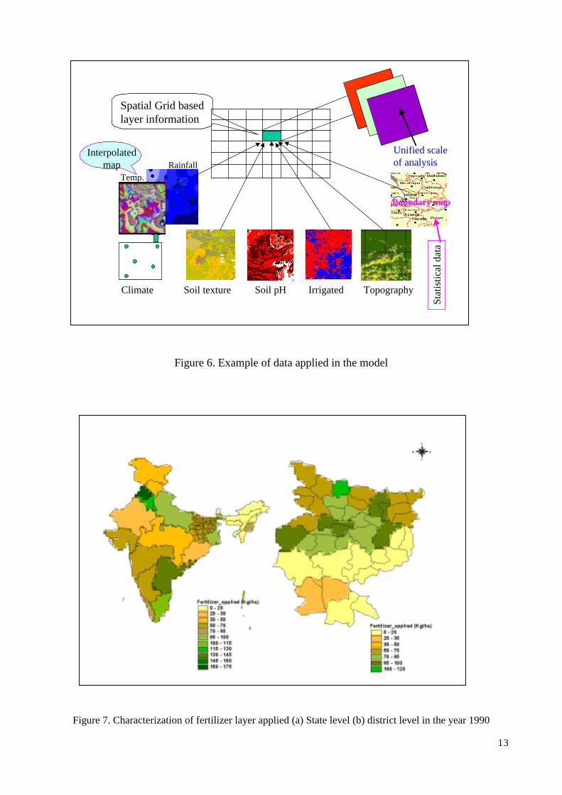
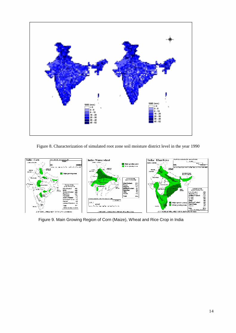
Bay of Bengal, in the north-east, north and a part of the north-west by Himalayan ranges, and the rest of the north-west by the Great Indian Desert. The soil characteristics of Indian nation obtained from different sources (like Survey of India and National Atlas Thematic Mapping Organization, NATMO) at national level in the form of maps (scale; 1:6 million) were used after digitization which has the properties like soil texture, soil pH and soil depth. All these soil properties were used in the form of layers for simulation. Slope information of the country was derived from 1km GTOPO (NGDC, 1997). Weather data were obtained and their surfaces were generated using World Meteorological Organization (WMO) station falling around 230 in number scattered throughout India. With the help of weather generator several layers were generated to feed the model, for example, minimum temperature, maximum temperature, rainfall, minimum and maximum standard deviation of temperatures and many more. Agricultural management data were obtained at state level where numbers of the states are more than 30 in total of entire India at 5 year interval which was used for coarse level whole country simulation of 50 km cell size. On the other hand we succeed in procuring time-series data from 1974-1994 for one of the Indian State Bihar for detailed study at finer resolution simulation of 10-km cell size. Figure 6 shows an example illustrating how the base data layers were used into simulation after unified scale of analysis. Also to show further characterization of some data layers figure 7 shows the amount of fertilizer used for the year 1990 in India at state and district level. Whereas, figure 8 shows the simulated root zone soil moisture as an intermediate output for the year 1970 and 1990 of entire country. With the help of above three figures (from 6 to 8) characterizations of different data layers derived/used after different analysis under simulation can be easily understood. 4. Results and Discussion The model developed in section 2 was found capable for simulating a number of crop management strategies, based on the selection and data provided by the user. It is a good contrast with site-specific original EPIC, where the management information given in the beginning continues for the total period of simulations year, hence the trend of output used to be more or less static and doesn’t correspond to the actual farm practice. An addition of dynamic adaptations had overcome this issue. Now with this, during computation, the model runs for each and every pixel following the rows and columns sequence with various multiple soil, climate, and management information provided in the form of layers. Two-year crop rotation was found appropriate for long term simulation. Two-year crop rotations were used. This proved to be better for the farmers to decide their productivity-based profit from the resources applied to continue the rotation or not. Hence, it was applied to impersonate more realistic simulation. The crops selected were maize-wheat-rice. These three crops were selected, as they are the first three main cereal crops from acrage and consumption in India. Crop management
6
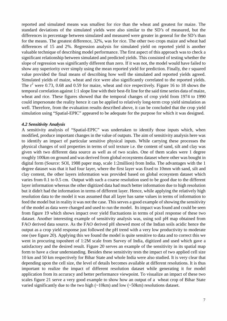
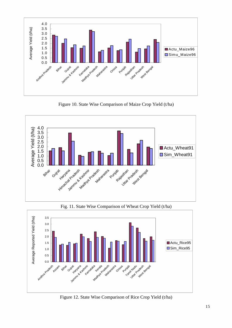
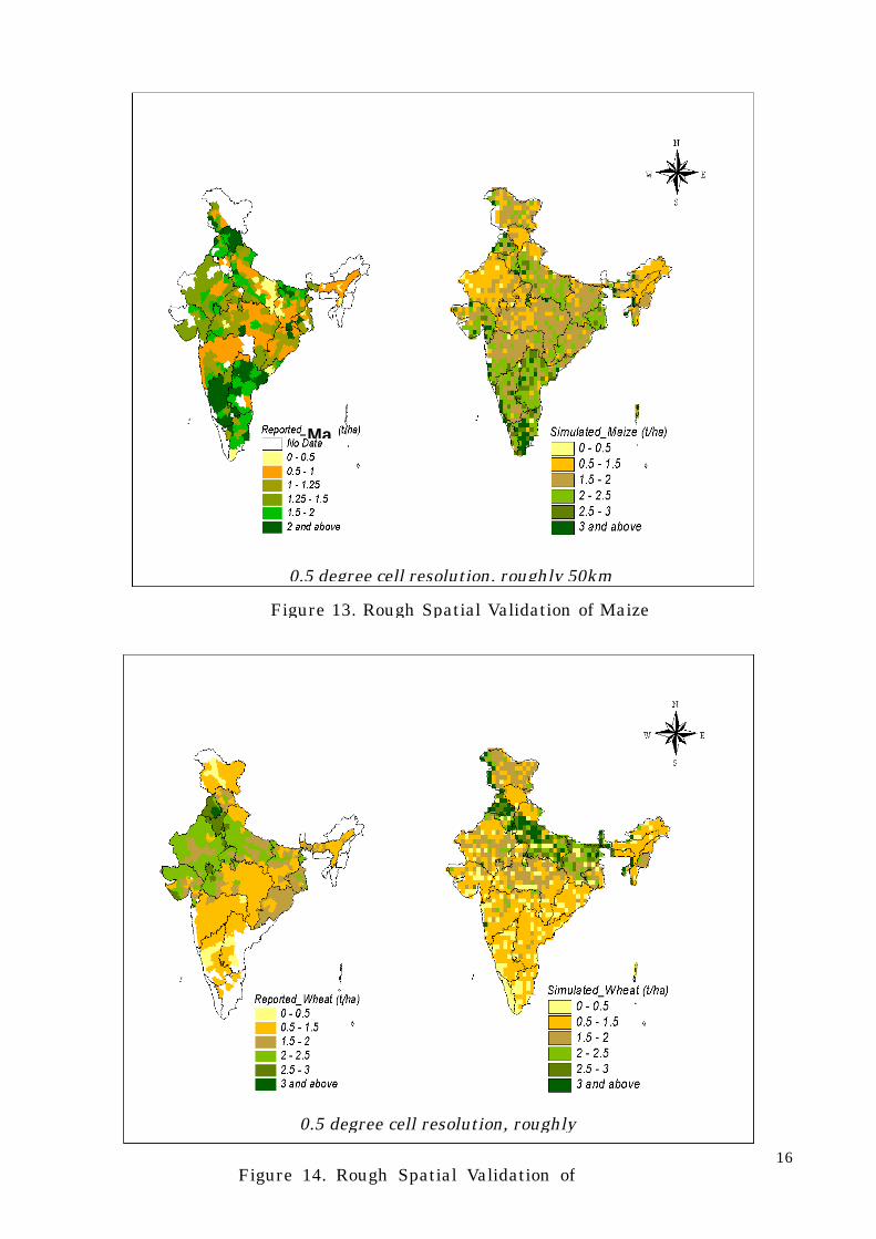
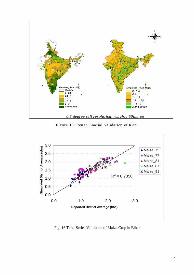
option supplied by user in the model can briefly be seen from figure 3 on its right hand side given management table. Besides these there are many other information which need to be fed like start of simulation date, planting date, harvesting date, tillage time, irrigation timing and its amount, fertilization time and so on. Amount of fertilizer applied was the reported state and district level data from 1975 to 1992 procured during the study. The crop selected in sequence for modelling was rainfed maize (without irrigation), irrigated wheat and monsoon rice. Possible measures explained above were taken into account to mimic the more realistic field practice. For better understanding of major and minor growing areas of these three crops in India, figure 9 can be referred with their planting and harvesting calendar. Yield simulation of the rainfed maize varied from 0.4 to 3.5 t/ha as shown in figure 10 described below under validation section for its spatial distribution of productivity throughout India. The maize yield shows high potentiality but being a third cereal it is not grown so widely like rice and wheat. Yield distribution of irrigated wheat crop varied between 0.5 to 3.5 t/ha also shown in figure 11 described below under validation section clears that mostly the northern part of India is the wheat belt. This is because the Indo-Gangetic plains form the most important wheat area. The cool winters and the hot summers are very conducive to a good crop of wheat, whereas the rice is being grown throughout India but the southern part of India forms most favorable season from agro-climatic conditions. The yield variation of monsoon rice was found to be fluctuating from 0. 3 to 3.0 t/ha. The spatial distribution of crop productivity output has been dealt in following validation section with its mapping/graphical representation to demonstrate the correspondence between simulated and reported crop yields. 4.1 Validation The first approach used to evaluate “Spatial-EPIC” yield simulation was to compare the output at state level average reported data for the year 1995 values. Closeness between measured and predicted yield at state level is the first and coarse level validation to see whether the simulated output is following the trend of reported aggregate average. For doing this, simulated 0.5 degree pixel resolution falling under the state were averaged and their mean were compared with the reported state level average shown in the form of bar chart from figure 10 to figure 12 for maize, wheat and rice crop respectively. Again to go further ahead at same resolution validation for whole India, the output for maize, rice and wheat for the year 1990 of these growing belts were compared by overlaying the district coverage. To extract the mean value of a district simulated yield; all pixels were overlaid with all India district boundaries, which are roughly 450 in number. All the pixels following under particular district were averaged and their computed means were compared with the average reported statistical value for these three crops. Spatial simulated vs. reported yield of maize, wheat and rice comparisons were helpful to find correspondence between growing region productivity. Although there were some places where model has simulated more or less yields in case of maize and rice whereas in general their simulated vs. reported values were close to each other (figure 13 to 15). The reason for getting less and more yields especially in rice crop is due to the limitation of not having district level time series data of entire nation instead we applied state level average management data (esp. fertilizer, figure 7). The above comparison demonstrates rough spatial cum average state level validation because of the fact that the applied management data for whole country simulations were state level average. The other approach used to evaluate “Spatial-EPIC” yield simulations was to compare the mean and standard deviation (SD) of the simulated yields of a crop with the same statistics for measured yields. Closeness between measured and predicted yields for these two statistics is important when making long-term decisions. This exercise was done for Bihar (one of the slightly north eastern Indian state) where time-series management data were applied as well as reported district level crop yield starting from year 1975 to 1994 made available. “Spatial-EPIC’s” mean simulated yields were found close to the reported mean yields (table 1). The mean differed by 12% or less. The difference between the
7
reported and simulated means was smallest for rice than the wheat and greatest for maize. The standard deviations of the simulated yields were also similar to the SD’s of measured, but the differences in percentage between simulated and measured were greater in general for the SD’s than for the means. The greatest difference, 32%, was for rice. The other two crops maize and wheat had differences of 15 and 2%. Regression analysis for simulated yield on reported yield is another valuable technique of describing model performance. The first aspect of this approach was to check a significant relationship between simulated and predicted yields. This consisted of testing whether the slope of regression was significantly different than zero. If it was not, the model would have failed to show any superiority over simply using the mean reported yield for prediction. Finally, the r squared
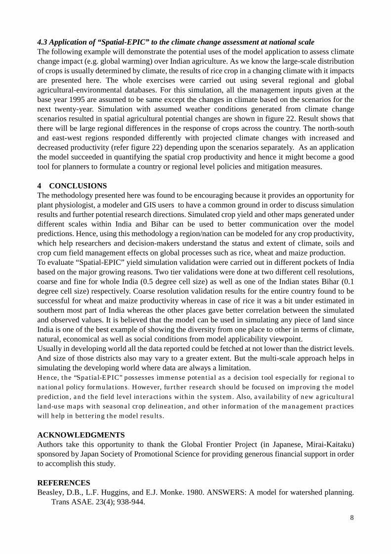
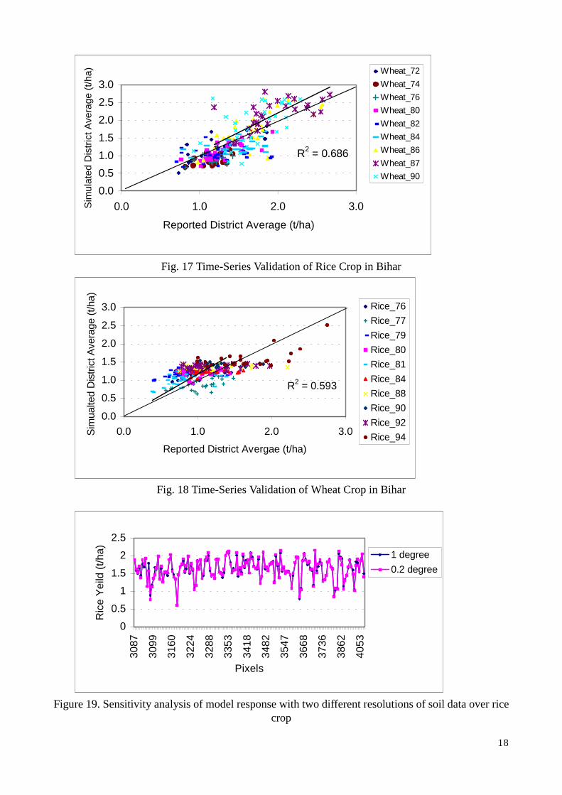
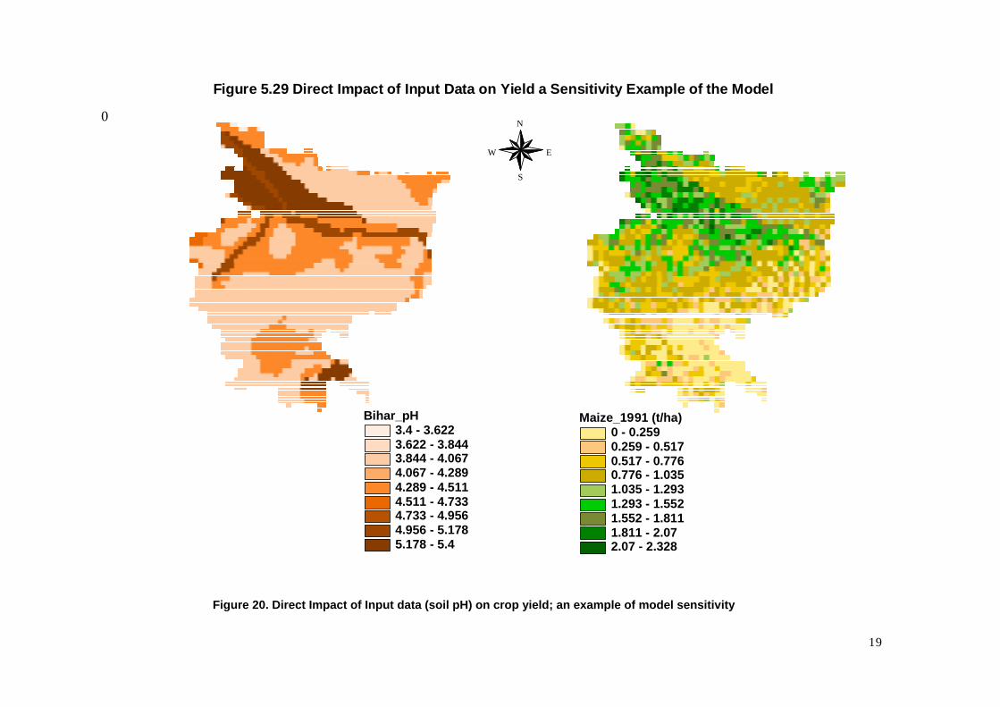
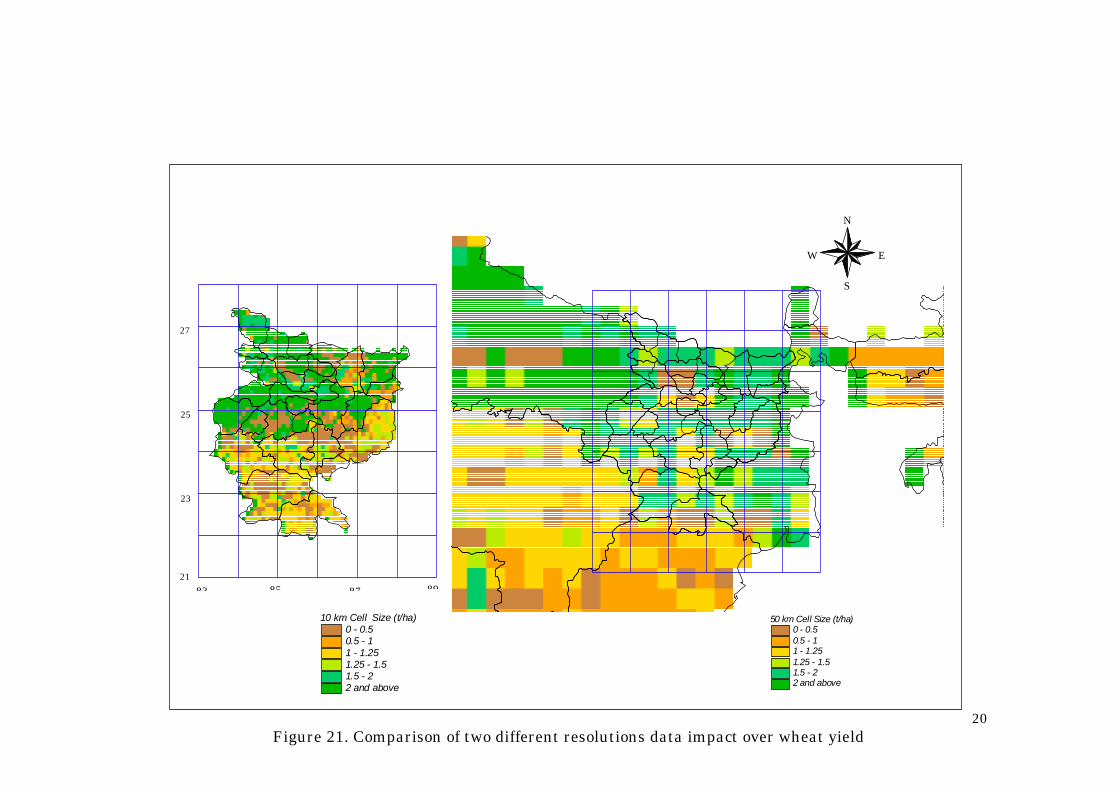
value provided the final means of describing how well the simulated and reported yields agreed. Simulated yields of maize, wheat and rice were also significantly correlated to the reported yields. The r2 were 0.73, 0.68 and 0.59 for maize, wheat and rice respectively. Figure 16 to 18 shows the temporal correlation against 1:1 slope line with their best-fit line for the said time series data of maize, wheat and rice. These figures showed that the temporal changes of crop yield from 1974 to 1990 could impersonate the reality hence it can be applied to relatively long-term crop yield simulation as well. Therefore, from the evaluation results described above, it can be concluded that the crop yield simulation using “Spatial-EPIC” appeared to be adequate for the purpose for which it was designed. 4.2 Sensitivity Analysis A sensitivity analysis of “Spatial-EPIC” was undertaken to identify those inputs which, when modified, produce important changes in the value of outputs. The aim of sensitivity analysis here was to identify an impact of particular sensitive physical inputs. While carrying these processes the physical changes of soil properties in terms of soil texture i.e. the content of sand, silt and clay was given with two different data source as well as of two scales. One of them scales were 1 degree roughly 100km on ground and was derived from global ecosystems dataset where other was bought in digital form (Source: SOI, 1988 paper map, scale 1:2million) from India. The advantages with the 1 degree dataset was that it had four layer, where the first layer was fixed to 10mm with sand, silt and clay content, the other layers information was provided based on global ecosystem dataset which varies from 0.1 to 0.5 cm. Output with such a coarse resolution used to be good due to the different layer information whereas the other digitized data had much better information due to high resolution but it didn't had the information in terms of different layer. Hence, while applying the relatively high resolution data to the model it was assumed that all layer has same values in terms of information to feed the model but in reality it was not the case. This serves a good example of showing the sensitivity of the model as data were changed and used to run the model. Its impact was found and could be seen from figure 19 which shows impact over yield fluctuations in terms of pixel response of these two dataset. Another interesting example of sensitivity analysis was, using soil pH map obtained from FAO derived data source. As the FAO derived pH showed most of the Indian soils acidic hence the output as a crop yield response just followed the pH trend with a very low productivity to moderate one (see figure 20). Applying this we found the model is quite sensitive to data and to correct this we went in procuring toposheet of 1:2M scale from Survey of India, digitized and used which gave a satisfactory and the desired result. Figure 20 serves an example of the sensitivity in its spatial map form to have a clear understanding. Besides these sensitivity tests the impact of two applied cell size 10 km and 50 km respectively for Bihar State and whole India were also studied. It is very clear that depending upon the cell size, the level of details becomes available at different resolutions. It is thus important to realize the impact of different resolution dataset while generating it for model application from its accuracy and better performance viewpoint. To visualize an impact of these two scales figure 21 serve a very good example to show how an output of a wheat crop of Bihar State varied significantly due to the two high (~10km) and low (~50km) resolutions dataset.
8
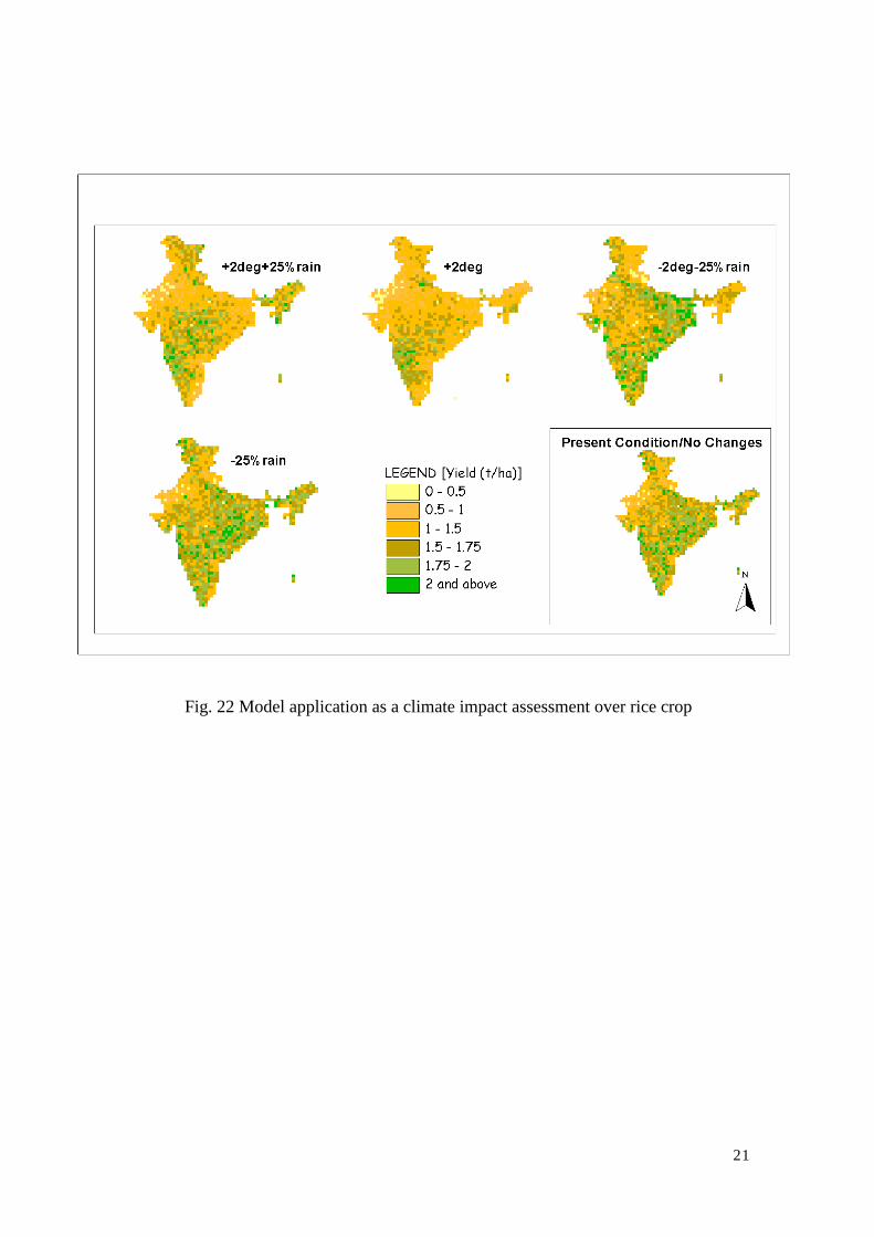
4.3 Application of “Spatial-EPIC” to the climate change assessment at national scale The following example will demonstrate the potential uses of the model application to assess climate change impact (e.g. global warming) over Indian agriculture. As we know the large-scale distribution of crops is usually determined by climate, the results of rice crop in a changing climate with it impacts are presented here. The whole exercises were carried out using several regional and global agricultural-environmental databases. For this simulation, all the management inputs given at the base year 1995 are assumed to be same except the changes in climate based on the scenarios for the next twenty-year. Simulation with assumed weather conditions generated from climate change scenarios resulted in spatial agricultural potential changes are shown in figure 22. Result shows that there will be large regional differences in the response of crops across the country. The north-south and east-west regions responded differently with projected climate changes with increased and decreased productivity (refer figure 22) depending upon the scenarios separately. As an application the model succeeded in quantifying the spatial crop productivity and hence it might become a good tool for planners to formulate a country or regional level policies and mitigation measures. 4 CONCLUSIONS The methodology presented here was found to be encouraging because it provides an opportunity for plant physiologist, a modeler and GIS users to have a common ground in order to discuss simulation results and further potential research directions. Simulated crop yield and other maps generated under different scales within India and Bihar can be used to better communication over the model predictions. Hence, using this methodology a region/nation can be modeled for any crop productivity, which help researchers and decision-makers understand the status and extent of climate, soils and crop cum field management effects on global processes such as rice, wheat and maize production. To evaluate “Spatial-EPIC” yield simulation validation were carried out in different pockets of India based on the major growing reasons. Two tier validations were done at two different cell resolutions, coarse and fine for whole India (0.5 degree cell size) as well as one of the Indian states Bihar (0.1 degree cell size) respectively. Coarse resolution validation results for the entire country found to be successful for wheat and maize productivity whereas in case of rice it was a bit under estimated in southern most part of India whereas the other places gave better correlation between the simulated and observed values. It is believed that the model can be used in simulating any piece of land since India is one of the best example of showing the diversity from one place to other in terms of climate, natural, economical as well as social conditions from model applicability viewpoint. Usually in developing world all the data reported could be fetched at not lower than the district levels. And size of those districts also may vary to a greater extent. But the multi-scale approach helps in simulating the developing world where data are always a limitation. Hence, the “Spatial-EPIC” possesses immense potential as a decision tool especially for regional to national policy formulations. However, further research should be focused on improving the model prediction, and the field level interactions within the system. Also, availability of new agricultural land-use maps with seasonal crop delineation, and other information of the management practices will help in bettering the model results. ACKNOWLEDGMENTS Authors take this opportunity to thank the Global Frontier Project (in Japanese, Mirai-Kaitaku) sponsored by Japan Society of Promotional Science for providing generous financial support in order to accomplish this study. REFERENCES Beasley, D.B., L.F. Huggins, and E.J. Monke. 1980. ANSWERS: A model for watershed planning.
Trans ASAE. 23(4); 938-944.
9
Botkin, D. B., Jank, J. F., and Wallis, J. R., 1972. Rationale, Limitations and Assumptions of a Northeastern Forest Growth Simulator: IBM Journal of Research and Development, Vol 16, pp. 101-116.
Dumesnil, D., ed. 1993. EPIC user’s guide-draft. USDA-ARS, Grassland, Soil and Water Research Laboratory, Temple, TX.
FAO/UNSESCO, 1995. Digital Soil Map of the World and Derived Soil Properties Version 3.5. Scale 1:5 million.
Global-View, Global Ecosystem Dataset, 1994. National Geophysical Data Center Boulder, Colorado, 80303, USA.
Godwin, D., Ritchie, J. T., Singh, U. and Hunt, L. 1989. A User's Guide to CERES-Wheat- V2.10. Muscle Shoals: International Fertilizer Development Center.
Grayson, R. B., 1992. Physically based hydrologic modelling. 2. Is the concept realistic? Water Resource 26(10):2659-2666.
Hann, C. T., B.J. Barfield, and J.C. Hayes, 1994. Hydrologic Modelling. In: Design Hydrology and Sedimentology for small catchments. Academic Press, Sand Diego, CA. 588 p.
IBSNAT, International Benchmark Sites Network for Agrotechnology Transfer Project, 1989. Decision Support System for Agrotechnology Transfer Version 21. (DSSAT V2.1), Dept Agronomy and Soil Sci.; College of Trop. Agr. And Human Resources; University of Hawaii, Honlolulu, HI 96822.
Jones, J. W., Boote, K. J., Hoogenboom, G., Jagtap, S. S. and Wilkerson, G. G. 1989. SOYGRO V5.42: Soybean Crop Growth Simulation Model. Users' Guide. Gainesville: Department of Agricultural Engineering and Department of Agronomy, University of Florida.
Kiniry, J. R., D. A. Spanel, J. R. Williams, and C. A. Jones 1990. Demonstration and validation of crop grain yield simulation by EPIC, USDA/ARS, Technical Bulletin Number 1768.
Knisel, W. G. 1980. CREAMS, A field scale model for chemicals, runoff, and erosion from agricultural management systems. U. S. Dept. of Agriculture, CRR-26. 643 pp.
Nemani, R.R, Running, S.W., Band, L.E., and Peterson, D.L., 1991. Regional Hydro-Ecological Simulation System – An illustration of the Integration of Ecosystem Models into a GIS in Pre-Conference Proceedings: First International Conference/Workshop on Integrating GIS and Environmental Models, Boulder, Coloardo, September 15-18, 1991.
NGDC, 1997. GTOPO30, Global Land One-Km Base Elevation, (Average 30-Second Elevations Grids). National Geophysical Data Center 325 Broadway, Boulder, Colorado.
Nisbet, R.A. , and Botkin, D.B., 1991. Integrating a Forest Growth Model with a Geographic Information System in Pre-Conference Proceedings: First International Conference/Workshop on Integrating GIS and Environmental Models, Boulder, Coloardo, September 15-18, 1991.
Ramnarayan, T.S., 1994. Performance of transport models in predicting nitrate in runoff flow in high water table areas. Presented at the 1994 International Summer Meeting Paper No. 94-2152, ASAE, St. Joseph, MI.
Richardson, C. W. (1981). Stochastic simulation of daily precipitation, temperature, and solar radiation. Water Resour. Res. 17(1): 81-92.
Running, S.W. and Coughlan, J.C. 1988. A General Model of Forest Ecosystem Processes for Regional Applications I-Hydrolgical Balance, Canopy Gas Exchange and Primary Production Processes: Ecological Modelling, Vol. 42 pp. 125-154.
Running, S.W., and Nemani, R.R., 1991. Regional Hydrological and Carbon Balance Response of Forests Resulting from Potential Climate Change: Climate Change, Vol. 19, pp.349-368.
Satya Priya Shibasaki, Ryosuke and Shiro Ochi, 1998. Modelling Spatial Crop Production: A GIS approach, Proceedings of the 19th Asian Conference on Remote Sensing, 16-20 Nov, 1998 held at Manila. pp A-9-1 to A-9-6. Schaller, N., 1990. Maintaining low input agriculture. J. Soil and Water Conservation 45:9-12. Schimel, D.S., and Burke, I.C., 1991. Spatial Interactive Models of Atmospheric Ecosystem
10
Coupling in Pre-Conference Proceedings: First International Conference/Workshop on Integrating GIS and Environmental Models, Boulder, Coloardo, September 15-18, 1991.
SOI. 1988. Survey of India paper map used for digitization of soil and soil acidity map. Williams, J. R. and . Sharpley, A.N., (eds.), 1989. EPIC --Erosion/Productivity Impact Calculator: 1.
Model Documentation, USDA Technical Bulletin No. 1768.
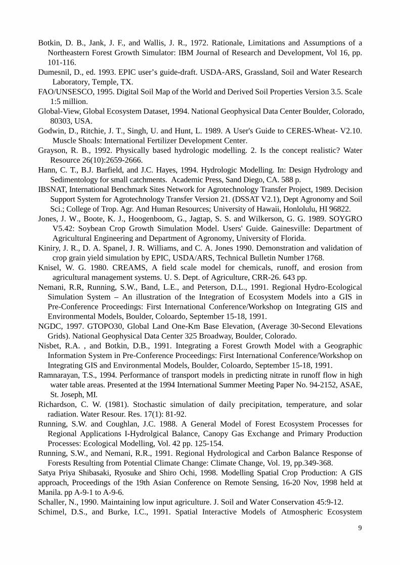
Table 1. Means and standard deviations of reported and simulated yields District_Average_Yield
Measured Simulated Crop Mean SD Mean SD r2 ----------------tons/ha----------------------- Maize 1.39 0.39 1.57 0.34 0.74 Wheat 1.47 0.29 1.34 0.46 0.68 Rice 1.24 0.19 1.14 0.26 0.59
Temperature
Radiation Precipitation
Tillage
Layered Soil Pedon
Percolation
Runoff Sediment
Chemicals a. Dissolved b. Adsorbed
Evapotransipration Wind
Figure 1. Physical Components of the Model
11
Figure 2. Modelling Linkage Diagram
Climatic DataNatural Resources
Elevation
Crops
Soils
SlopeRainfall
Temp.
HRU Coveragecurve no. (CN)
Management PracticeCrop Fert. Irrig. HRU
Spatial-EPIC
Crop Yield RZSW
Figure 3. Brief schematic Presentation of modelling under “Spatial-EPIC”
12
Figure 4. Concept of ‘weather’ generator (generating high resolution temporal daily data from coarse
resolution monthly data.)
Figure 5. Concept of ‘slope’ generator (deriving the range and impact of two resolution DEM computed slope over soil loss)
0
0 0.2 0.4
Variability of soil loss caused usingcoarse resolution DEM
Slop
e gr
adie
nt fr
om c
oars
e re
solu
tion
DE
M (e
.g.1
0km
)
015 10 5
0.2
Soil Loss (mm)
0
0.6
Slope gradient from fine resolution DEM(e.g. 1km)
20
0.4
-0.4 -0.2
0.2
0.4
0.0
-0.2
-0.4
Abs
olut
e sl
ope
grad
ient
in d
egre
es
Slope gradient from coarseresolution DEM
Variability of fineresolution slope gradient
0 5
10 15 20 25 30 35 40 45 50
1 26 51 76 10 12 15 17 20 22 25 27 30 32 35Days
daily_temp monthly_temp
Daily weather conditions
Monthly data (coarse resolution)
Statistical analysis
Stochastic generation of “fine” resolution data
Temp
13
Figure 6. Example of data applied in the model
Figure 7. Characterization of fertilizer layer applied (a) State level (b) district level in the year 1990
Climate Soil texture Soil pH Topography
Interpolatedmap
Stat
istic
al d
ata
Spatial Grid basedlayer information
Unified scaleof analysis
Boundary map
Irrigated
RainfallTemp.
14
Figure 8. Characterization of simulated root zone soil moisture district level in the year 1990
Figure 9. Main Growing Region of Corn (Maize), Wheat and Rice Crop in India
15
Figure 10. State Wise Comparison of Maize Crop Yield (t/ha)
Fig. 11. State Wise Comparison of Wheat Crop Yield (t/ha)
Figure 12. State Wise Comparison of Rice Crop Yield (t/ha)
0.00.51.01.52.02.53.03.54.0
Andhra
Prades
hBiha
rGujr
at
Jammu &
Kashm
ir
Karnata
ka
Madhy
a Prad
esh
Mahara
stra
Orissa
Punjab
Rajasth
an
Uttar P
rades
h
West B
enga
l
Aver
age
Yiel
d (t/
ha)
Actu_Maize96Simu_Maize96
0.00.51.01.52.02.53.03.54.0
Bihar
Gujrat
Haryan
a
Himac
hal P
rades
h
Jammu &
Kashm
ir
Madhy
a Prad
esh
Mahara
stra
Punjab
Rajasth
an
Uttar P
rades
h
West B
enga
l
Aver
age
Yiel
d (t/
ha)
Actu_Wheat91Sim_Wheat91
0.0
0.5
1.0
1.5
2.0
2.5
3.0
3.5
Andhra
Prades
h
Assam Biha
rGujr
at
Haryan
a
Jammu &
Kashm
ir
Karnata
kaKera
la
Madhy
a Prad
esh
Mahara
stra
Orissa
Punjab
Tamil N
adu
Uttar P
rades
h
West B
enga
l
Aver
age
Rep
orte
d Yi
eld
(t/ha
)
Actu_Rice95Sim_Rice95
16
Figure 13. Rough Spatial Validation of Maize
0.5 degree cell resolution, roughly 50km
Ma
0.5 degree cell resolution, roughly
Fig. 11
Figure 14. Rough Spatial Validation of
17
Fig. 16 Time-Series Validation of Maize Crop in Bihar
0.5 degree cell resolution, roughly 50km on
Figure 15. Rough Spatial Validation of Rice
R2 = 0.7356
0.0
0.5
1.0
1.5
2.0
2.5
3.0
0.0 1.0 2.0 3.0Reported District Average (t/ha)
Sim
ulat
ed D
istr
ict A
vera
ge (t
/ha) Maize_75
Maize_77Maize_81Maize_87Maize_91
18
Fig. 17 Time-Series Validation of Rice Crop in Bihar
Fig. 18 Time-Series Validation of Wheat Crop in Bihar
Figure 19. Sensitivity analysis of model response with two different resolutions of soil data over rice crop
R2 = 0.686
0.00.51.01.52.02.53.0
0.0 1.0 2.0 3.0Reported District Average (t/ha)
Sim
ulat
ed D
istri
ct A
vera
ge (t
/ha) Wheat_72
Wheat_74Wheat_76Wheat_80Wheat_82Wheat_84Wheat_86Wheat_87Wheat_90
R2 = 0.593
0.0
0.5
1.0
1.5
2.0
2.5
3.0
0.0 1.0 2.0 3.0Reported District Avergae (t/ha)
Sim
ualte
d D
istri
ct A
vera
ge (t
/ha)
Rice_76Rice_77Rice_79Rice_80Rice_81Rice_84Rice_88Rice_90Rice_92Rice_94
00.5
11.5
22.5
3087
3099
3160
3224
3288
3353
3418
3482
3547
3668
3736
3862
4053
Pixels
Ric
e Ye
ild (t
/ha) 1 degree
0.2 degree
19
0
Bihar_pH3.4 - 3.6223.622 - 3.8443.844 - 4.0674.067 - 4.2894.289 - 4.5114.511 - 4.7334.733 - 4.9564.956 - 5.1785.178 - 5.4
N
EW
S
Maize_1991 (t/ha)0 - 0.2590.259 - 0.5170.517 - 0.7760.776 - 1.0351.035 - 1.2931.293 - 1.5521.552 - 1.8111.811 - 2.072.07 - 2.328
Figure 5.29 Direct Impact of Input Data on Yield a Sensitivity Example of the Model
Figure 20. Direct Impact of Input data (soil pH) on crop yield; an example of model sensitivity
20
50 km Cell Size (t/ha)0 - 0.50.5 - 11 - 1.251.25 - 1.51.5 - 22 and above
N
EW
S
Map 5.4 Comparision of Two Different Resolutions Impact Over Wheat Yield
10 km Cell Size (t/ha)0 - 0.50.5 - 11 - 1.251.25 - 1.51.5 - 22 and above
Spatial Resolution10 x 10 degree(~ 10 x 10 km)
Spatial Resolution50 x 50 degree(~ 50 x 50 km)
83 85 87 8921
23
25
27
Figure 21. Comparison of two different resolutions data impact over wheat yield
21
Fig. 22 Model application as a climate impact assessment over rice crop