NAVAL POSTGRADUATE · PDF fileA. NAVAL AVIATION METROLOGY AND CALIBRATION ... Metrology and Calibration Definitions ... Naval Postgraduate School

NAVAL POSTGRADUATE

SCHOOL

MONTEREY, CALIFORNIA

MBA PROFESSIONAL REPORT

Increasing Operational Availability of H-60 Calibration Support Equipment

By: Kenneth D. Bevel,

Kelly M. Johnson, and Robert N. Stonaker

December 2006

Advisors: Keebom Kang Uday M. Apte

Approved for public release; distribution is unlimited.

THIS PAGE INTENTIONALLY LEFT BLANK

i

REPORT DOCUMENTATION PAGE Form Approved OMB No. 0704-0188 Public reporting burden for this collection of information is estimated to average 1 hour per response, including the time for reviewing instruction, searching existing data sources, gathering and maintaining the data needed, and completing and reviewing the collection of information. Send comments regarding this burden estimate or any other aspect of this collection of information, including suggestions for reducing this burden, to Washington headquarters Services, Directorate for Information Operations and Reports, 1215 Jefferson Davis Highway, Suite 1204, Arlington, VA 22202-4302, and to the Office of Management and Budget, Paperwork Reduction Project (0704-0188) Washington DC 20503. 1. AGENCY USE ONLY

2. REPORT DATE December 2006

3. REPORT TYPE AND DATES COVERED MBA Professional Report

4. TITLE AND SUBTITLE: Increasing Operational Availability of H-60 Calibration Support Equipment 6. AUTHOR(S) Kenneth Bevel, Kelly Johnson, and Robert Stonaker

5. FUNDING NUMBERS

7. PERFORMING ORGANIZATION NAME(S) AND ADDRESS(ES) Naval Postgraduate School Monterey, CA 93943-5000

8. PERFORMING ORGANIZATION REPORT NUMBER

9. SPONSORING / MONITORING AGENCY NAME(S) AND ADDRESS(ES) N/A

10. SPONSORING / MONITORING AGENCY REPORT NUMBER

11. SUPPLEMENTARY NOTES The views expressed in this report are those of the author(s) and do not reflect the official policy or position of the Department of Defense or the U.S. Government. 12a. DISTRIBUTION / AVAILABILITY STATEMENT Approved for public release; distribution is unlimited

12b. DISTRIBUTION CODE A

13. ABSTRACT

The purpose of this MBA Project was to identify inefficiencies in the H-60 support equipment calibration process at Naval Air Station, North Island and analyze their impact on operational availability. To conduct this analysis, the researchers mapped the standard calibration process at North Island from beginning to end from a using unit perspective. After identifying the process, the researchers calculated the inherent and operational availability and determined the impacts of process inefficiencies on asset operational availability. The researchers proposed changes to reduce the effects of process inefficiencies on using unit asset availability and provided guidance for further study.

15. NUMBER OF PAGES

94

14. SUBJECT TERMS Calibration, Support Equipment, Operational Availability, Process Inefficiencies

16. PRICE CODE

17. SECURITY CLASSIFICATION OF REPORT

Unclassified

18. SECURITY CLASSIFICATION OF THIS PAGE

Unclassified

19. SECURITY CLASSIFICATION OF ABSTRACT

Unclassified

20. LIMITATION OF ABSTRACT

UL NSN 7540-01-280-5500 Standard Form 298 (Rev. 2-89) Prescribed by ANSI Std. 239-18

ii


iii

Approved for public release; distribution is unlimited

INCREASING OPERATIONAL AVAILABILITY OF H-60 CALIBRATION SUPPORT EQUIPMENT

Kenneth D. Bevel, Captain, United States Marine Corps Kelly M. Johnson, Captain, United States Marine Corps

Robert N. Stonaker, Captain, United States Marine Corps

Submitted in partial fulfillment of the requirements for the degree of

MASTER OF BUSINESS ADMINISTRATION

from the

NAVAL POSTGRADUATE SCHOOL December 2006

Authors: _____________________________________

Kenneth D. Bevel _____________________________________

Kelly M. Johnson

_____________________________________ Robert N. Stonaker

Approved by: _____________________________________

Keebom Kang, Co-Advisor _____________________________________ Uday M. Apte, Co-Advisor _____________________________________ Robert N. Beck, Dean

Graduate School of Business and Public Policy

iv


v

INCREASING THE OPERATIONAL AVAILABILITY OF H-60 CALIBRATION SUPPORT EQUIPMENT

ABSTRACT

The purpose of this MBA Project was to identify inefficiencies in the H-60

support equipment calibration process at Naval Air Station, North Island, and analyze

their impact on operational availability. To conduct this analysis, the researchers mapped

the standard calibration process at North Island from beginning to end from a using unit

perspective. After identifying the process, the researchers calculated the inherent and

operational availability and determined the impacts of process inefficiencies on asset

operational availability. The researchers proposed changes to reduce the effects of

process inefficiencies on using unit asset availability and provided guidance for further

study.

vi


vii

TABLE OF CONTENTS

I. INTRODUCTION........................................................................................................1 A. BACKGROUND ..............................................................................................1 B. PURPOSE.........................................................................................................2 C. RESEARCH QUESTION ...............................................................................2 D. SCOPE ..............................................................................................................2 E. ORGANIZATION OF STUDY ......................................................................3

II. CALIBRATION PROCESS .......................................................................................5 A. NAVAL AVIATION METROLOGY AND CALIBRATION

PROGRAM ......................................................................................................5 1. Metrology and Calibration Definitions..............................................5 2. Metrology and Calibration Program (METCAL) ............................5

a. Navy Primary Standards Laboratory (NPSL)..........................6 b. Navy Depot Calibration Laboratory (NDCL) ..........................7 c. Field Calibration Activities (FCA) ...........................................7

B. NAVAL AVIATION CALIBRATION ..........................................................8 C. NORTH ISLAND CALIBRATION PROCESS............................................8

a. Sub-Custodian Calibration Process Responsibilities ..............8 b. Customer Activity Calibration Process Responsibilities..........9 c. Calibration Facility Responsibilities ......................................11

III. DATA SOURCING....................................................................................................15 A. DATA FROM MOCC ...................................................................................15 B. DATA FROM THE SQUADRONS .............................................................15 C. MOCC DESCRIPTION ................................................................................16 D. MOCC CALIBRATION PROCESS RESPONSIBILITIES .....................16 E. MEASURE DESCRIPTION.........................................................................17

IV. METHODOLOGY ....................................................................................................19 A. OVERVIEW...................................................................................................19 B. KEY MEASURE ENTRIES .........................................................................19 C. ESTABLISHING THE FIVE VARIBLES USED TO EXPRESS THE

CALIBRATION PROCESS .........................................................................20 1. The Variable X ...................................................................................20 2. The Variable Y ...................................................................................20 3. The Variable V ...................................................................................20 4. The Variable W..................................................................................20 5. The Variable Z ...................................................................................21

D. SCENARIOS DECREASING OPERATIONAL AVAILABILITY.........21 1. Inherent Availability Scenario..........................................................21 2. Early Asset Turn-in ...........................................................................22 3. Late Asset Turn-in .............................................................................24 4. Comparing Early versus Late Equipment Turn-ins.......................26

viii

5. Delayed Delivery to the Using Unit ..................................................26 6. Increases in the Processes of Y and V ..............................................28

E. DATA PREPARATION................................................................................29 1. Scrubbing and Sorting the MEASURE Data ..................................30

a. Eliminating Administrative Lines ..........................................30 b. Sorting the Data ......................................................................30

2. Defining the Variables X, Y, V, W, and Z in the MEASURE Data .....................................................................................................30 a. The Value of X ........................................................................30 b. The Value of Y.........................................................................31 c. The Value of V ........................................................................31 d. The Value of W .......................................................................32 e. The Value of Z.........................................................................32

3. Filtering the Data ...............................................................................33 a. Focusing on the North Island Calibration

Laboratories/Activities (NIQ and SDB) .................................33 b. Filtering the Equipment Condition Category ........................33 c. Filtering the Service Label Category......................................34 d. Filtering the Work Performed On-Site category ...................36 e. Filtering of Equipment Status ................................................36 f. Filtering Calculated Values of the Metrology Cycle .............36

F. APPLYING THE SCENARIOS TO THE DATA ......................................37 1. Inefficiencies from Early Turn-ins ...................................................37

a. Reduced Operational Availability...........................................37 b. Additional Calibration Manpower Hours ..............................38 c. Additional Manpower Needed for Early Calibrations...........39 d. Unrealized Support Equipment Value ...................................40

2. Inefficiencies from Late Turn-ins.....................................................40 a. Reduced Operational Availability...........................................41 b. Reduced Equipment Value .....................................................41

3. Reduction from Process Delays Following Calibration..................41

V. ANALYSIS .................................................................................................................43 A. INTRODUCTION..........................................................................................43 B. DATA OVERVIEW.......................................................................................43

1. Servicing Lab......................................................................................44 2. Equipment Condition ........................................................................44 3. Service Label ......................................................................................45 4. Work Performed on Site ...................................................................45 5. Equipment Status...............................................................................45 6. Metrology Cycles................................................................................45 7. Summary.............................................................................................46

C. OVERALL REDUCTIONS IN OPERATIONAL AVAILABILITY .......46 1. Trends in Early versus Late Turn-ins..............................................47 2. Trends in the Values of Y, V, W.......................................................47 3. Trends in the Values of X..................................................................47

ix

4. Trends in the Values of Z ..................................................................48 5. Trends in Ai and Ao............................................................................48

D. HYPOTHETICAL ANALYSIS....................................................................48 E. ADDITIONAL MANPOWER HOURS NEEDED FOR EARLY

CALIBRATIONS...........................................................................................49 F. OPERATIONAL AVAILABILITY REDUCTIONS OF SPECIFIC

CALIBRATION ASSETS.............................................................................50

VI. CONCLUSION AND RECOMMENDATIONS.....................................................53 A. CONCLUSION ..............................................................................................53 B. RECOMMENDATIONS...............................................................................53

1. Limit Turn-In Inefficiencies Through Policy Change....................53 2. Change the Navy’s Method of Assigning METR Cycles................55 3. Implementation of Information Technology Systems ....................57

C. FURTHER STUDY .......................................................................................58 1. Increase the Length of Metrology Intervals ....................................58 2. Work Center 67A...............................................................................59 3. Monitor Support Equipment Throughout the Calibration

Process.................................................................................................59 4. Calibration Support Equipment Repair and Maintenance

Process.................................................................................................59

APPENDIX A. MEASURE FORMAT 802................................................................61

APPENDIX B. CALIBRATION CYCLE..................................................................63

APPENDIX C. HYPOTHETICAL TURN-IN ANALYSIS .....................................65

LIST OF REFERENCES......................................................................................................67

INITIAL DISTRIBUTION LIST .........................................................................................71

x


xi

LIST OF FIGURES

Figure 1. Calibration Process at the Sub-Custodian Level................................................9 Figure 2. MEASURE Recall Process (DoN, OPNAV OP43P6B, n.d.)..........................10 Figure 3. Calibration Process from the Sub-Custodian to the NDCL or FCA................10 Figure 4. Calibration Process at the Calibration Facility ................................................13 Figure 5. MEASURE Inventory Cycle............................................................................17 Figure 6. Graph of Ao with Changing Values of Z .........................................................26 Figure 7. Graph of Ao with Increasing Values of W.......................................................28 Figure 8. Graph of Ao with Increasing Values of the Variables Y or V .........................29 Figure 9. Reliability of a Single Calibration Asset Considered Independently ..............56 Figure 10. Reliability of Multiple Calibration Assets Considered in Parallel...................56

xii


xiii

LIST OF TABLES

Table 1. Data Overview .................................................................................................44 Table 2. Overall Operational Availability Chart............................................................47 Table 3. Losses Due to Additional Calibration Man Hours...........................................49 Table 4. Unrealized Value in the Triaxial Accelerometer .............................................50 Table 5. Unrealized Value in the Single Axis Accelerometer .......................................50 Table 6. Regulation of Z for Early Turn-ins ..................................................................54 Table 7. Regulation of Z for Late Turn-ins....................................................................54 Table 8. No Z Greater than 14 Days for Late and Early Turn-ins .................................55

xiv


xv

LIST OF EQUATIONS

Equation 1. Inherent Availability ........................................................................................22 Equation 2. Numerical Example of Ai ................................................................................22 Equation 3. Early Turn-in Operational Availability............................................................23 Equation 4. Numerical Example of Early Turn-in Operational Availability ......................24 Equation 5. Late Turn-In Operational Availability .............................................................25 Equation 6. Numerical Example of Late Turn-In Operational Availability........................25 Equation 7. Delayed Delivery Operational Availability .....................................................27 Equation 8. Numerical Example of Delayed Delivery Operational Availability................27 Equation 9. Reduced Operational Availability from Early Turn-in....................................38 Equation 10. Numerical Example of Reduced Operational Availability from Early

Turn-in .............................................................................................................38 Equation 11. Additional Calibration Manpower Hours Required.........................................39 Equation 12. Numerical Example of Hours Added to Calibration Cycle .............................39 Equation 13. Example Reduction in Equipment Value.........................................................40 Equation 14. Reduced Operational Availability From Late Turn-in.....................................41 Equation 15. Numerical Example of Reduced Operational Availability due to Late

Turn-in .............................................................................................................41 Equation 16. Reduced Operational Availability From Process Delays Following

Calibration........................................................................................................42 Equation 17. Numerical Example of Reduced Operational Availability due to Process

Delays Folloing Calibration.............................................................................42

xvi


xvii

LIST OF ACRONYMS AND ABBREVIATIONS

AIMD Aircraft Intermediate Maintenance Detachment CDBF Central Database Facility CHMSWP Commander of Helicopter Marine Strike Wing Pacific COMNAVAIRFOR Commander Naval Air Forces COMNAVAIRFORINST Commander Naval Air Forces Instruction DoD Department of Defense DoN Department of the Navy ECN Equipment Control Number EIRT Equipment Identification and Receipt Tag FCA Field Calibration Activity HSL Helicopter Anti Submarine Squadron HSM Helicopter Maritime Strike Squadron IMA Intermediate Maintenance Activity LPO Leading Petty Officer MAGTF Marine Air-Ground Task Force MEASURE Metrology Engineering Automated System for Uniform

Recall and Reporting METCAL Metrology and Calibration METCALREP Metrology and Calibration Representative METER Metrology Equipment Recall and Report METR Metrology MOCC Measure Operational Control Center NAMP Naval Aviation Maintenance Program

xviii

NAS Naval Air Station NAVAIR Naval Air Systems Command NAVAIRSYSCOM Naval Air Systems Command NAVSEA Naval Sea Systems Command NDCL Naval Depot Calibration Laboratory NIST National Institute of Standards and Technology NIQ Naval Air Station, North Island Field Calibration Facility NPSL Navy Primary Standards Laboratory NWSC Naval Surface Warfare Center OPNAV Office of the Chief of Naval Operations PME Precision Measuring Equipment SE Support Equipment SECNAV Secretary of the Navy SDB Naval Air Rework Facility, North Island TAMS Test and Monitoring Systems USMC United States Marine Corps

xix

ACKNOWLEDGMENTS

The researchers would like to thank our advisors for their guidance. They would

also like to thank the operating personnel in the calibration process for their time and

patience, with special thanks to the MOCC and the maintenance personnel at HSM-41

and HSL-43. Finally, the researchers would like to thank their spouses for their support.

xx


1

I. INTRODUCTION

A. BACKGROUND

In the past, the Calibration Industry hailed the Navy’s Calibration and Metrology

service as some of the most technologically advanced services rendered by the military.

Over the past 60 years, the United States Navy strived to create a consistent standard for

calibration in support of the Naval forces. The Navy’s objectives for creating metrology

and calibration standards were to increase combat readiness, reduce maintenance costs,

and provide the combat forces with the most advanced support equipment that yield

optimal performance and operational availability. Unfortunately, the Navy’s calibration

and metrology service has not updated the calibration process in order to keep pace with

the technological and policy advances in the industry. While some personnel may view

the Navy’s calibration and metrology services as superior, other patrons at Naval

Aviation Station (NAS) North Island, California, identified the calibration process as

inefficient with regards to turnaround time and the operational availability of support

equipment. The present challenge is to identify methods to continually improve the

calibration and metrology processes to meet the needs of a changing military with

shrinking resources.

The researchers initiated this project based on the work of Lieutenant Tim

Snowden, USN, and Lieutenant Commander Doug Sullivan, USN, in the project titled

Filling H-60 Helicopter Readiness Shortfalls by Streamlining and Revising Depot Level

Maintenance Procedures. Following-up this project, the researchers visited the

Commander of Helicopter Marine Strike Wing Pacific (CHMSWP) in March of 2006.

The commander relayed his frustration towards the calibration process. His claim was

that the metrology cycles for his calibration support equipment (SE) were too short.

After a brief conversation, the researchers toured the calibration facilities at NAS North

Island, CHMSWP’s home port. During this tour, the researchers examined the

calibration processes and looked for inefficient, as well as, efficient practices.

2

Upon further analysis, the following question emerged: Can reducing

inefficiencies in the calibration process significantly increase the operational availability

of SE?

B. PURPOSE

The purpose of this project was to examine the SE calibration process from the

using unit perspective to discover key process inefficiencies and determine their impacts

on operational availability.

C. RESEARCH QUESTION

According to Naval Aviation units at North Island, the current calibration process

from the sub-custodian to the field calibration activity (FCA) and Naval Depot

Calibration Laboratory (NDCL) produces inefficient results for its patrons. The

questions that will be answered are: What are the key inefficiencies in the calibration

process at NAS, North Island, and can improvements in these inefficiencies significantly

improve the operational availability of the calibration SE?

D. SCOPE

This report focuses on the operational availability (Ao) of the calibration SE

equipment for two Naval Aviation units at North Island, Helicopter Maritime Strike

Squadron Forty-One (HSM-41) and Helicopter Anti Submarine Squadron Light Forty-

Three (HSL-43). As defined by OPNAVINST 3000.12A, operational availability

“…provides a measure of time or probability that a system’s capabilities will be available

for operational use when needed. The researchers analyzed the calibration process at

NAS North Island and concluded that three scenarios may have a significant effect on SE

operational availability.

• Early Turn-ins from the sub-custodian to the designated calibration facility.

• Late Turn-ins from the sub-custodian to the designated calibration facility.

3

• Delays created by entities in the calibration process from the designated calibration facility to sub-custodian.

The researchers examined each scenario to determine the effects of early turn-ins,

late turn-ins, and process delays on the operational availability of support equipment.

After analyzing the effects, the researchers recommended changes to improve the

operational availability of SE and reduce inefficiencies in the calibration process.

E. ORGANIZATION OF STUDY

This project is six chapters. Chapter II includes a literature review of the Naval

Aviation METCAL Program and the Naval Aviation Maintenance Program, as well as an

explanation of the North Island Calibration Process. Chapter III outlines the various

sources of the researcher’s data and their respective missions in the Navy. Chapter IV

presents a simplified model of the calibration process, establishes the variables the

researchers utilized to express the process, outlines the scenarios that decrease the

operational availability of SE, describes how the researchers prepared the data, and how

the researchers applied the scenarios to the data. Chapter V provides an overview of the

data, discusses trends in the overall operational availability, and analyzes specific SE

inefficiencies. Chapter VI presents the conclusion, offers overall recommendations to

increase the operational availability of SE, and recommends avenues of further analysis.

4


5

II. CALIBRATION PROCESS

A. NAVAL AVIATION METROLOGY AND CALIBRATION PROGRAM

This chapter lists the Navy definitions of calibration and metrology, and also

includes the purposes of the METCAL program. The researchers established this base of

knowledge to provide an overview of the Navy regulations before focusing on the

specific calibration process at NAS North Island.

1. Metrology and Calibration Definitions

Metrology is the science of measurement or determination of conformance to

technical requirements and the development of standards and systems for absolute and

relative measurements. Calibration is the process by which calibration installations

compare a calibration standard or precision measuring equipment (PME) with a standard

of higher accuracy to ensure the former is within specified limits throughout its entire

range. (Department of the Navy [DoN], COMNAVAIRFORINST 4790.2, 2005) The

Navy uses metrology to determine the adequate technical requirements for a system and

then uses calibration to measure those technical requirements against a system of

unknown accuracy. The quantitative measurements allow SE to operate safely and

efficiently within the established tolerances noted in NAVAIR 17-35MTL-1.

2. Metrology and Calibration Program (METCAL)

The Secretary of the Navy (SECNAV) established the METCAL Program to

support the Navy’s metrology and calibration requirements. The METCAL Program

provides the operating forces the calibration and repair facilities that ensure optimum

performance of calibrated SE. (DoN, N88-NTSP-A-50-8701B/A, 2000) The calibration

facilities compare the SE to metrology standards of higher accuracy to create uniform and

traceable measurements with links to the National Institute of Standards and Technology

(NIST), the U.S. Naval Observatory, or another Department of Defense (DoD) approved

calibration facility. The primary technical authority for the METCAL Program is the

6

Measurement Science Department at the Naval Surface Warfare Center (NSWC) in

Corona, California. The core functions of the Measurement Science Department are the

following:

• Provide Navy-wide technical direction, support, and guidance relating to measurement requirements for Test and Monitoring Systems (TAMS) to Naval Sea Systems Command (NAVSEA), Naval Air Systems Command (NAVAIR), Strategic Systems Program, and Marine Corps Metrology and Acquisitions Program Offices. (DoN, Naval Surface Warfare Center [NWSC], 2006)

• Evaluate measurement and calibration requirements for a wide range of Navy programs and systems, both domestic and Foreign Military Sales. (DoN, NWSC, 2006)

• Establish, document, and sustain Navy calibration support requirements including test parameters, required calibration equipment, support documentation, servicing intervals, logistic support levels, and calibration training requirements. (DoN, NWSC, 2006)

• Perform engineering studies and analyses to assure that measurement traceability requirements are achieved. (DoN, NWSC, 2006)

• Provide technical guidance, review, and approval to Navy activities and contractors in the development of Integrated Logistics Support Plans, Life-Cycle Support Planning, calibration source data, and similar documents related to the Navy METCAL Program. (DoN, NWSC, 2006)

While NWSC provides guidance and instruction for calibration and metrology

services, NAVAIR 17-35NCA-1 delineates which level of calibration facility will

conduct the calibration and repair of each type of support equipment. The three

calibration levels that support Naval calibration activities.

a. Navy Primary Standards Laboratory (NPSL)

NPSL is the Fleet Support Activity for calibration standards. NPSL

maintains direct liaison with NIST and the Naval Observatory to ensure measurements

are traceable. The purpose of NPSL is to provide critical metrology engineering services

for support equipment and TAMS outside the capabilities of lower echelon calibration

laboratories, and supply as a repository for Navy primary standards (DoN, N88-NTSP-A-

50-8701B/A, 2000).

7

b. Navy Depot Calibration Laboratory (NDCL)

NDCL provides calibration and repair of metrology standards and SE that

are beyond the capability of lower echelon calibration laboratories. The National Bureau

of Standards, via NPSL, provides the calibration and metrology repair standards to

NDCL. (DoN, N88-NTSP-A-50-8701B/A, 2000) The NDCL also provides ashore and

afloat calibration services to NAVAIRSYSCOM.

c. Field Calibration Activities (FCA)

Combining both afloat and ashore numbers, the Navy operates

approximately 100 Intermediate Maintenance Activities (IMAs). (DoN, N88-NTSP-A-

50-8701B/A, 2000) Within the IMAs, the Navy established and designated Work

Centers 67A, and designated calibration laboratories as FCAs. Military personnel, versus

civilian, primarily operate the FCAs. Their mission is to provide intermediate level

calibration and repairs of any fleet SE and metrology standards for which they maintain

standards and instrument calibration procedures. (DoN, N88-NTSP-A-50-8701B/A,

2000)

The three levels of calibration facilities work together to provide

customers with current calibration requirements and use the latest tools and technology to

increase equipment readiness and reduced maintenance cost.

The METCAL program assigns each asset a laboratory code. That

specific laboratory is responsible for conducting the calibration and repair of that asset.

One goal of the METCAL program is to support the concept of “calibrating at the lowest

level possible.” (DoN, COMNAVAIRFORINST 4790.2, 2005) This concept allows

simple calibrations to remain at the lower levels of maintenance, while allowing the

higher echelons of maintenance to focus on more critical or complex calibration

requirements.

8

B. NAVAL AVIATION CALIBRATION

The Commander Naval Air Forces (COMNAVAIRFOR) outlined the use of the

calibration program in the Naval Aviation Maintenance Program (NAMP) manual to

support the Navy’s metrology and calibration goals. The purpose of

COMNAVAIRFOR’s directives is to coordinate the proper use of the METCAL program

at the organizational, intermediate and depot level maintenance. “The objective of the

NAMP is to achieve and continually improve aviation material readiness and safety

standards established by the Chief of Naval Operations and COMNAVAIRFOR, with

coordination from the Commandant of the Marine Corps focusing on the optimal use of

manpower, material, facilities and funds.” (DoN, COMNAVAIRFORINST 4790.2, 2005)

The NAMP outlines the responsibilities, policies and requirements for the three levels of

maintenance as they relate to metrology and calibration. The purpose for outlining the

procedures is to guarantee uniform, relevant, and traceable calibration processes.

C. NORTH ISLAND CALIBRATION PROCESS

The calibration facilities at NAS North Island have the capability to provide

intermediate and depot level calibration. For the purpose of this project, the researchers

focused on the calibration procedures from the sub-custodian to the intermediate and

depot-level calibration facilities. In the following sub-sections, the researchers outlined

the responsibilities of each entity in the calibration process. These responsibilities

provide more clarity to the overall calibration process.

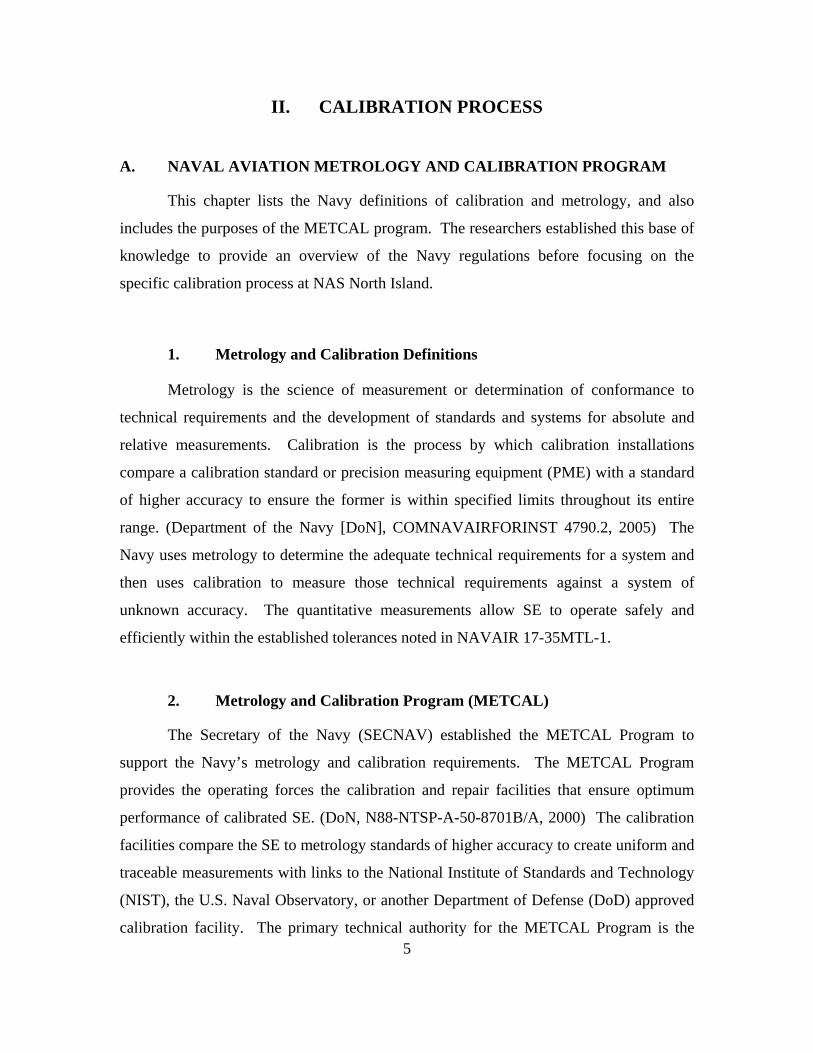
a. Sub-Custodian Calibration Process Responsibilities

The sub-custodian, as defined by the NAMP manual, is “…a MEASURE

participant supported by a customer activity that has physical custody of equipment,

regardless of actual ownership.” (DoN, COMNAVAIRFORINST 4790.2, 2005)

According to the calibration process at NAS North Island, HSM-41 and HSL-43 are sub-

custodians. The sub-custodian’s calibration responsibilities begin with the acceptance of

MEASURE format 802. (See Appendix B) According to the MEASURE users manual

(OPNAV OP43P6B), the sub-custodian retrieves the MEASURE recall format 802 from

9

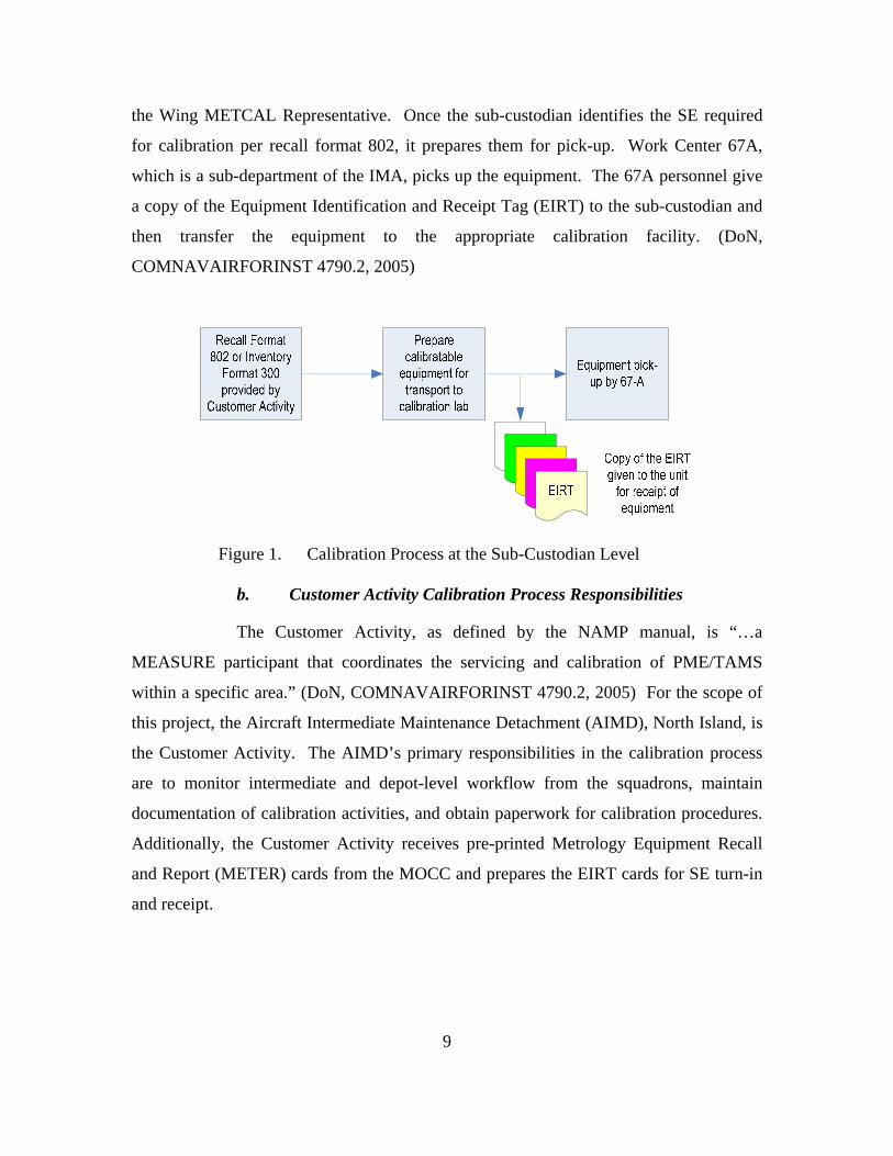
the Wing METCAL Representative. Once the sub-custodian identifies the SE required

for calibration per recall format 802, it prepares them for pick-up. Work Center 67A,

which is a sub-department of the IMA, picks up the equipment. The 67A personnel give

a copy of the Equipment Identification and Receipt Tag (EIRT) to the sub-custodian and

then transfer the equipment to the appropriate calibration facility. (DoN,

COMNAVAIRFORINST 4790.2, 2005)

Figure 1. Calibration Process at the Sub-Custodian Level

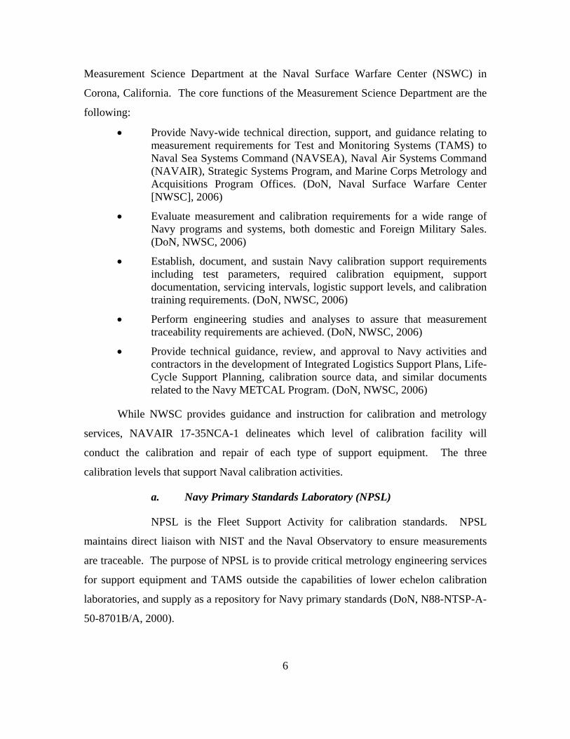
b. Customer Activity Calibration Process Responsibilities

The Customer Activity, as defined by the NAMP manual, is “…a

MEASURE participant that coordinates the servicing and calibration of PME/TAMS

within a specific area.” (DoN, COMNAVAIRFORINST 4790.2, 2005) For the scope of

this project, the Aircraft Intermediate Maintenance Detachment (AIMD), North Island, is

the Customer Activity. The AIMD’s primary responsibilities in the calibration process

are to monitor intermediate and depot-level workflow from the squadrons, maintain

documentation of calibration activities, and obtain paperwork for calibration procedures.

Additionally, the Customer Activity receives pre-printed Metrology Equipment Recall

and Report (METER) cards from the MOCC and prepares the EIRT cards for SE turn-in

and receipt.

10

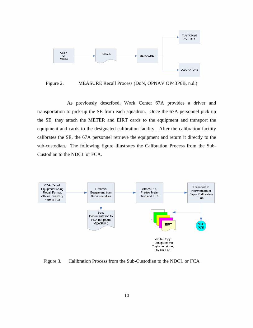
Figure 2. MEASURE Recall Process (DoN, OPNAV OP43P6B, n.d.)

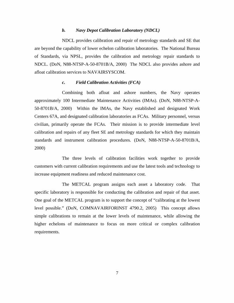
As previously described, Work Center 67A provides a driver and

transportation to pick-up the SE from each squadron. Once the 67A personnel pick up

the SE, they attach the METER and EIRT cards to the equipment and transport the

equipment and cards to the designated calibration facility. After the calibration facility

calibrates the SE, the 67A personnel retrieve the equipment and return it directly to the

sub-custodian. The following figure illustrates the Calibration Process from the Sub-

Custodian to the NDCL or FCA.

Figure 3. Calibration Process from the Sub-Custodian to the NDCL or FCA

11

c. Calibration Facility Responsibilities

The Calibration Facility, as defined by the NAMP manual, is “…an

installation under the control of military departments or any agency of DoD.” (DoN,

COMNAVAIRFORINST 4790.2, 2005) It provides calibration services for PME and

calibration standards used by activities engaged in the following activities:

• Research

• Development

• Test and Evaluation

• Production

• Quality Assurance

• Maintenance

• Supply

• The Operation of weapons system(s), equipment, and other DoD material. (DoN, COMNAVAIRFORINST 4790.2, 2005)

For this project, the researchers investigated the calibration services

provided by the FCA and the NDCL at NAS North Island. As previously mentioned, the

FCA is an intermediate-level calibration facility that provides calibration services to

MEASURE participants. NAS North Island’s FCA (listed as “NAS North Island” in

NAVAIR 12-35NCA-1) conducts calibration activities for the sub-custodians and

oversees the establishment of a PME/TAMS production control work center (67A).

Additionally, the facility controls the flow of calibration equipment from the sub-

custodians to the intermediate and depot-level calibration facilities. (DoN,

COMNAVAIRFORINST 4790.2, 2005) The NDCL is a depot-level calibration facility

that provides metrology and calibration services to MEASURE participants. For North

Island, the depot level calibration facility is Naval Air Rework Facility

(NAVAIREWORK), which conducts calibration and metrology services for units afloat

and ashore. According to NAVAIR 17-35NCA-1, the laboratory code for NAS North

Island is NIQ and the laboratory code for NAVAIREWORK is SDB.

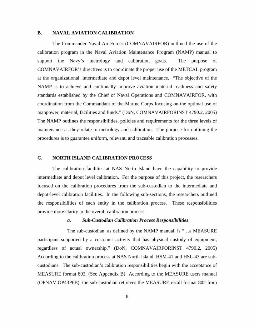
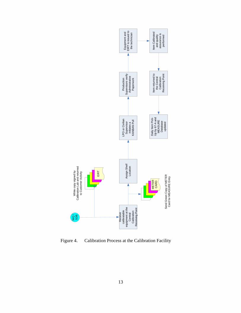
SDB and NIQ have similar roles in the calibration process at NAS North

Island. At this point, 67A brings the SE to the shipping and receiving area of NIQ or

12

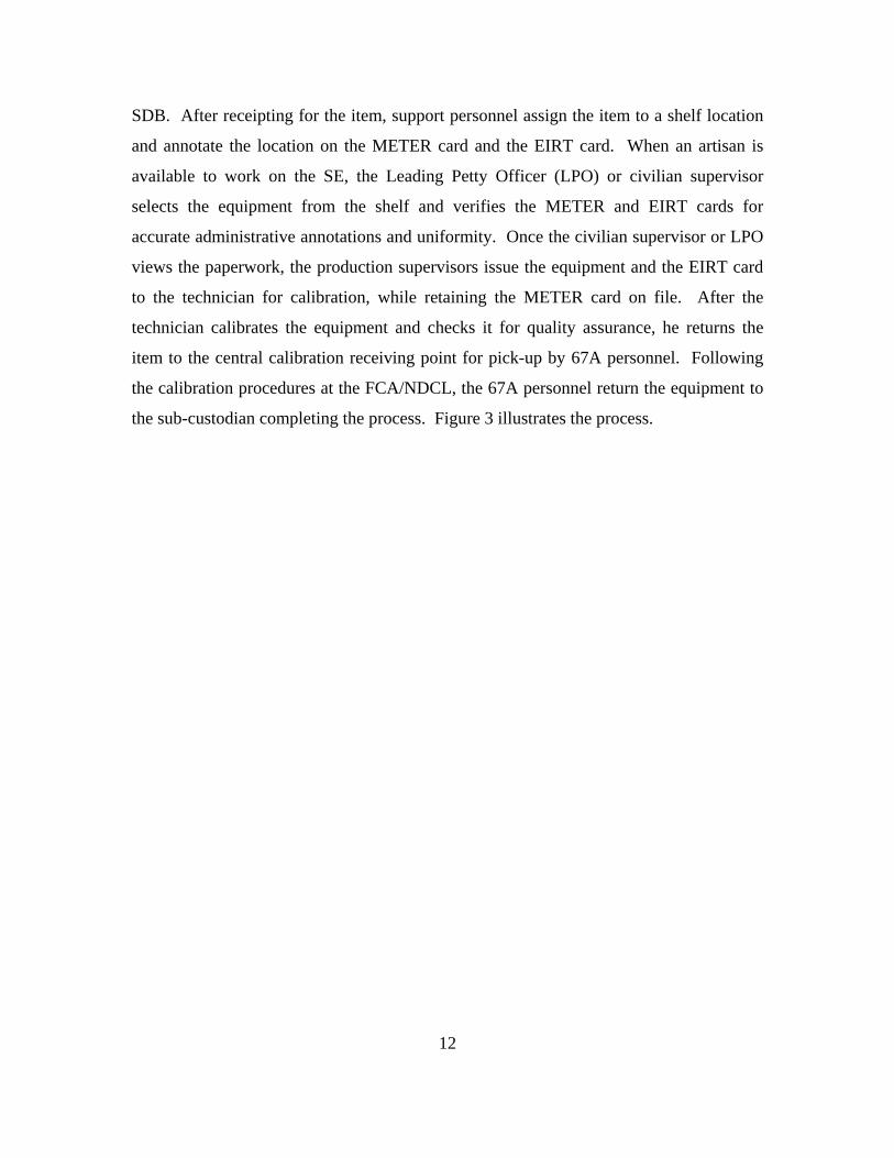
SDB. After receipting for the item, support personnel assign the item to a shelf location

and annotate the location on the METER card and the EIRT card. When an artisan is

available to work on the SE, the Leading Petty Officer (LPO) or civilian supervisor

selects the equipment from the shelf and verifies the METER and EIRT cards for

accurate administrative annotations and uniformity. Once the civilian supervisor or LPO

views the paperwork, the production supervisors issue the equipment and the EIRT card

to the technician for calibration, while retaining the METER card on file. After the

technician calibrates the equipment and checks it for quality assurance, he returns the

item to the central calibration receiving point for pick-up by 67A personnel. Following

the calibration procedures at the FCA/NDCL, the 67A personnel return the equipment to

the sub-custodian completing the process. Figure 3 illustrates the process.

13

Rec

eive

ca

libra

tabl

e eq

uipm

ent a

t the

C

entra

l C

alib

ratio

n R

ecei

ving

Poi

nt

Ass

ign

She

lf Lo

catio

n

LPO

or C

ivili

an

Sup

ervi

sor

initi

ates

a

KAN

BAN

Pul

l

Pro

duct

ion

Sup

ervi

sors

ver

ify

Adm

inis

trativ

e P

aper

wor

k

Equ

ipm

ent a

nd

EIR

T is

issu

ed to

th

e te

chni

cian

NIQ

/ SD

B

EIR

T

Whi

te c

opy

sign

ed b

y C

alib

ratio

n La

b an

d re

turn

ed

to C

usto

mer

Act

ivity

ME

TER

CA

RD

Sen

d G

reen

Cop

y of

ME

TER

C

ard

for M

EAS

UR

E E

ntry

Item

Cal

ibra

ted

and

qual

ity

assu

ranc

e is

pe

rform

ed

Item

retu

rned

to

the

Cen

tral

Cal

ibra

tion

Rec

eivi

ng P

oint

Dal

iy It

em P

ick-

Up

by 6

7-A

and

M

EAS

UR

E D

atab

ase

upda

ted

Figure 4. Calibration Process at the Calibration Facility

14


15

III. DATA SOURCING

A. DATA FROM MOCC

A representative from the MOCC NAS, North Island provided the researchers

with the MEASURE data from HSM-41 and HSL-43 in the form of an excel spreadsheet.

The data covered the period from March 1998 through May 2006. The researchers

sequentially narrowed the fields of data within the excel file to view only the datum

relevant to the SE calibration process. The researchers will discuss a detailed description

of MEASURE in Section D of this chapter.

B. DATA FROM THE SQUADRONS

HSM-41 and HSL-43 are SH-60/MH-60R Helicopter Squadrons located at NAS,

North Island. The researchers randomly selected both squadrons. The mission of HSM-

41 is “To train Naval aviators and Naval aircrew personnel to employ the SH-60B and

MH-60R aircraft in conducting offensive and defensive anti-submarine and surface

warfare operations in littoral regions and at sea, in a high-density, multi-threat

environment.” (Helicopter Maritime Strike Squadron Forty-One [HSM-41], 2006) The

mission of HSL-43 is to “Qualify, train, and deploy fully combat-ready detachments

onboard U.S. warships. (Helicopter Anti Submarine Squadron Light Forty-Three [HSL-

43], 2006) When ashore at North Island, both HSL-43 and HSM-41 follow the same

calibration asset turn-in/receipt process as described in Chapter II. Each squadron

utilizes the same type of Recall Schedule that the MOCC provides. The researchers

describe the Recall Schedule in Section F of this chapter.

Along with the MEASURE data the researchers received from the MOCC, HSM-

41 and HSL-43 each provided data illustrating the 10 most often broken SE as well as the

20 most often utilized SE. In Chapter IV, the researchers applied the results from various

operational availability analyses to this set of data to illustrate the specific impacts that

early and late turn-ins have on the operational availability of these equipments.

16

C. MOCC DESCRIPTION

The MOCC operates as a Government Owned Contractor Operated activity, and

provides several services to METCAL customers. First and foremost, MOCC personnel

operate the MEASURE program, which ultimately aides the sub-custodians in the

schedule and recall of their SE. The MOCC maintains current and accurate data and

process methodologies. By maintaining updated Information Technology, the MOCC

provides the sub-custodian an efficient and cost-effective means of reaching mission

objectives. MOCC personnel work hand-in-hand with the METCAL representatives to

manage and oversee the calibration process among the units stationed at NAS, North

Island. (MOCC, personal communication, October 4, 2006)

D. MOCC CALIBRATION PROCESS RESPONSIBILITIES

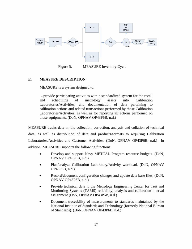
The initial process for a using unit to establish documentation into MEASURE

begins with the completion of inventory forms containing all calibration assets owned by

the Customer Activity that will enter the calibration process. The appropriate Metrology

Calibration Representative (METCALREP) verifies these forms and then forwards the

documents to the appropriate MOCC, or Central Database Facility (CDBF) if a MOCC is

not available, for documentation into MEASURE. The Customer Activity receives a

printed inventory along with the preprinted METER cards that accompany the calibration

asset during the turn-in phase of the calibration process. The METCALREP initiates the

last stage of the initial MEASURE Inventory Cycle by providing the Customer Activity

and Calibration Activity/Laboratory with a one month projected Recall Schedule of

calibration assets due in for calibration. Figure 2-1 illustrates this process. (DoN,

OPNAV OP43P6B, n.d.)

17

Figure 5. MEASURE Inventory Cycle

E. MEASURE DESCRIPTION

MEASURE is a system designed to:

…provide participating activities with a standardized system for the recall and scheduling of metrology assets into Calibration Laboratories/Activities, and documentation of data pertaining to calibration actions and related transactions performed by those Calibration Laboratories/Activities, as well as for reporting all actions performed on those equipments. (DoN, OPNAV OP43P6B, n.d.)

MEASURE tracks data on the collection, correction, analysis and collation of technical

data, as well as distribution of data and products/formats to requiring Calibration

Laboratories/Activities and Customer Activities. (DoN, OPNAV OP43P6B, n.d.) In

addition, MEASURE supports the following functions:

• Develop and support Navy METCAL Program resource budgets. (DoN, OPNAV OP43P6B, n.d.)

• Plan/analyze Calibration Laboratory/Activity workload. (DoN, OPNAV OP43P6B, n.d.)

• Record/document configuration changes and update data base files. (DoN, OPNAV OP43P6B, n.d.)

• Provide technical data to the Metrology Engineering Center for Test and Monitoring Systems (TAMS) reliability, analysis and calibration interval assignment (DoN, OPNAV OP43P6B, n.d.)

• Document traceability of measurements to standards maintained by the National Institute of Standards and Technology (formerly National Bureau of Standards). (DoN, OPNAV OP43P6B, n.d.)

18

Simply stated, the MEASURE system provides MEASURE participants with an

accurate picture of the SE calibration process as well as useful historical data for future

analysis.

19

IV. METHODOLOGY

A. OVERVIEW

Beyond the anecdotal stories, the researchers needed to find data that could clarify

whether or not the calibration process contained inefficient practices. Through the use of

the MEASURE data as well as the descriptions from the key parties involved, the

researchers created a simplified process flow chart illustrating the standard calibration

process at SDB or NIQ. Appendix C illustrates this simplified process.

B. KEY MEASURE ENTRIES

The following bullets list the key MEASURE time entries the researchers utilized

to track the calibration process. Appendix C illustrates where each time entry occurs in

the calibration process.

• DT_RCVD – This entry denotes the date the Calibration Laboratory/Activity received the SE from 67A personnel. (DoN, OPNAV OP43P6B, n.d.)

• DT_INDCT – This entry denotes the date the artisan at the Calibration Laboratory/Activity initiated work on the equipment and inducted it into the calibration maintenance cycle. (DoN, OPNAV OP43P6B, n.d.)

• DT_CMPL – This entry denotes the date the artisan at the Calibration Laboratory/Activity completed work on the equipment and returned it to the receiving area for out-processing. (DoN, OPNAV OP43P6B, n.d.)

• DT_PROC – This entry denotes the date 67A personnel retrieved the asset from the Calibration Laboratory/Activity. (MOCC, personal communication, October 16, 2006 )

• DT_NXTDUE – This is the date equipment is due to return to the facility for a subsequent calibration. MEASURE automatically enters this date based on the metrology cycle and the date the artisan completed working on the asset (DT_CMPL). (DoN, OPNAV OP43P6B, n.d.)

20

C. ESTABLISHING THE FIVE VARIBLES USED TO EXPRESS THE CALIBRATION PROCESS

After analyzing the standard calibration procedures, the researchers established

five variables to express different elements in calibration process. Appendix C illustrates

the order and duration of each variable in the process

1. The Variable X

The variable X represents the Metrology (METR) cycle for the SE. The METR

cycle is the number of days the end user may utilize the equipment after an approved

calibration laboratory/activity verifies the standard of calibration. In the researcher’s

data, the length of the METR cycles ranged from 3 to 60 months, with a mean of 15.7

months and a mode of 12 months.

2. The Variable Y

The variable Y represents the average value added calibration process time. It

begins when an artisan inducts the SE into the calibration process and ends when an

artisan finishes all work on the equipment and establishes a new METR cycle. In this

project, the researchers assumed that the duration an artisan works on SE is value added

time. In the researcher’s data, the length of the process times ranged from 0 to 253 days,

with a mean of 6.52 days and a mode of 0 days.

3. The Variable V

The variable V represents the delay that occurs after a using unit releases the SE

into the calibration cycle, but before an artisan inducts the equipment into maintenance.

In the researcher’s data, the length of these delays ranged from 1 to 161 days, with a

mean of 4.85 days and a mode of 1 day.

4. The Variable W

The variable W represents the delay that occurs from when the artisan completes

calibration on the SE (establishing a new METR cycle), to when the using unit regains

21

custody of the equipment. In the researcher’s data, the length of these delays ranged

from 1 to 111 days with a mean of 4.22 days and a mode of 2 days.

5. The Variable Z

The variable Z represents the number of days the using unit releases the

equipment from their custody either before or after the expiration of the METR cycle. In

the researchers’ data, the values of this variable ranged from 1,088 days early (or -1,088)

to 1,472 days late. While the average value of Z for the researcher’s data was -87 days,

or 87 days early, the average deviation from zero (the average absolute value of Z) was

107 days. The mode for this variable was -1, or 1 day early. Once again, Appendix C

provides a visual overview of the calibration cycle and also portrays the scope of each of

the previously described variables.

D. SCENARIOS DECREASING OPERATIONAL AVAILABILITY

The underlying problem in the calibration process is the variability in the turn in

of the SE. When the Navy first procured the equipment, it designed a standard

operational availability based on the prescribed metrology cycles for each type of SE.

Unfortunately, when equipment arrives early or late to the calibration facility, the

operational availability of that equipment decreases. Additionally, the availability

decreases for every delay that the equipment experiences in its return trip to the squadron.

These three types of inefficiencies amount to all of the possible ways a using unit can

reduce equipment operational availability. In the following sub-sections, the researchers

will use the five variables outlined in the previous section to express the three possible

reductions in operational availability.

1. Inherent Availability Scenario

The following equation represents the Inherent Availability (Ai) for the process.

The Ai equation includes the available useful equipment time and the value-added

22

maintenance functions and excludes administrative and logistics functions. (DoN,

OPNAVINST 3000.12A, 2003) As described earlier, X equals the METR cycle for the

SE, Y equals the average process time. Assuming V, W, and Z equal zero, the

operational availability is as follows:

XA X Yi = +

Equation 1. Inherent Availability

The following equation represents a numerical example of the Ai. Assuming a

base scenario of a 3-month or 90-day METR cycle (X) and a 10-day maintenance process

(Y), the Ai is as follows:

90 0.990 10

Ai = =+

Equation 2. Numerical Example of Ai

The resulting Ai is 90%.

2. Early Asset Turn-in

The squadrons turn in SE to the Calibration Laboratory/Activity early when they

suspect the equipment is out of calibration standards. The researchers identified three

general scenarios when the squadrons suspect the SE is out of standard and turn the

equipment in early for calibration. The first scenarios are due to “technicalities,”

like if the calibration sticker located on the SE becomes illegible or detaches before

the end of the METR cycle. The information on the calibration sticker is pertinent to

the accurate use of the SE, and if it becomes illegible, Navy regulations require the

using units to re-calibrate the equipment, even though the equipment’s current METR

23

cycle has not expired. These situations usually result over a long period of time, and

with SE that the using unit uses frequently.

The second scenarios result when the using unit physically shocks the equipment,

or compromises calibration seals. Once again, the Navy requires the using unit to re-

calibrate the equipment because such actions could easily affect the SE’s calibration

settings. These scenarios often occur when the using unit personnel accidentally drop the

equipment. Although the previous scenarios require the using units to turn in the

equipment early, these scenarios account for a small percentage of the early turn-ins.

Most early turn-ins arise from a third scenario.

The third scenarios arise when the using units turn-in the SE early on their own

volition. Examples of these scenarios include when using units want the equipment to

start a deployment cycle with a new calibration, or to renew the calibration on equipment

the using units infrequently use. (METCAL Rep, personal communication, November 6,

2006)

The following equation represents a scenario where a using unit turns in SE to the

Calibration Laboratory/Activity early, before the expiration of the METR cycle.

- --X Z WAo X Z Y V

=+ +

Equation 3. Early Turn-in Operational Availability

As before, X equals the METR cycle and Y equals the value added time at the

Calibration Laboratory/Activity. In this scenario, the variable V equals the delay

processing the SE to the Calibration Laboratory/Activity, the variable W equals delay

returning the SE to the using unit following calibration, and variable Z equals the number

of days the squadron turns the SE in early, before the expiration of the METR cycle. The

researchers subtract the value of Z from X in the numerator and the denominator because

the using unit looses these days from the METR cycle and the entire cycle as a whole.

The maintenance process days in “Y” remain the same in the equation. An example of

24

this scenario would be a unit re-establishing the METR cycle for tools prior to

deployment by turning the asset in “Z” days before the METR cycle expired.

Assume the same base scenario values from the previous numerical example,

where X is a 90-day METR cycle and Y is a 10-day maintenance cycle. For simplicity,

assume the variables W and V are zero. Assuming a Z value of 5 days, i.e., a scenario

where the squadron enters the SE into the cycle 5 days before the expiration of the METR

cycle, the resulting operational availability is as follows:

90 5 0 .89590 5 10 0

Ao− −

= =− + +

Equation 4. Numerical Example of Early Turn-in Operational Availability

The resulting Ao is 89.5% operational availability.

3. Late Asset Turn-in

The squadrons turn-in SE late for several reasons. The first scenarios result from

administrative oversight. Using unit personnel simply forget to turn in the equipment on

time. The operational tempo plays a factor in this situation. The next scenarios result

when using units turn in equipment late because they wait until after returning from

deployment. The using units could turn in the equipment aboard ship for calibration, but

choose to hold on to the equipment until the ship returns to home port. The next

scenarios are also related to deployments. Errors in tracking account for late turn-ins as

well. Currently, the MOCC sends calibration reports to deployed using units via physical

mail. These reports show dates the SE is due for calibration. Sometimes, the mail

process delays or losses these reports. The last scenarios arise from the transfer of

equipment between the homeguard squadrons and their deploying detachments.

Currently, the homeguard squadrons do not have visibility of the SE once they transfer it

to the deploying detachment. The loss of visibility could result in inefficient turn-in

processes.

25

The following equation represents late turn-in, or a scenario where a squadron

enters SE into the calibration process several days after the equipment’s METR cycle

expires. An example of this scenario would be if a mechanic neglected a tool in the shop

bench until the next time he needed it. At that time, he realized that the equipment

needed to be recalibrated and entered it into the calibration cycle. The resulting equation

would look like the following:

X WAo X Y V Z−

=+ + +

Equation 5. Late Turn-In Operational Availability

In this scenario, the using unit uses the tool for the full METR cycle, so the value of X

does not decrease as in the early turn-in example. Instead, the using unit adds additional

time onto the cycle by maintaining possession of the equipment following the expiration

of the METR cycle. Unlike the previous scenario (Early Turn-in), the numerator does not

change by the value of X like the denominator. The reason for this difference is as

follows: Although the using unit increases the overall process cycle by Z days when it

maintains possession beyond the METR cycle length, Navy regulations stipulate it cannot

use the asset beyond the expiration of the METR cycle. Assuming the base scenario

values for X and Y, V and W equal to zero, and a Z equal to a 5 day delay, the

operational availability equation would look like the following:

90 0 .85790 10 5 0

Ao−

= =+ + +

Equation 6. Numerical Example of Late Turn-In Operational Availability

The resulting Ao is 85.7% operational availability.

26

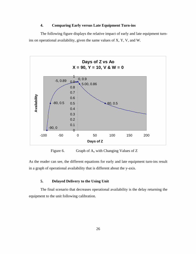
4. Comparing Early versus Late Equipment Turn-ins

The following figure displays the relative impact of early and late equipment turn-

ins on operational availability, given the same values of X, Y, V, and W.

Days of Z vs AoX = 90, Y = 10, V & W = 0

-5, 0.895.00, 0.86

0, 0.9

-90, 0

-80, 0.5 80, 0.5

00.10.20.30.40.50.60.70.80.9

1

-100 -50 0 50 100 150 200

Days of Z

Ava

ilabi

lity

Figure 6. Graph of Ao with Changing Values of Z

As the reader can see, the different equations for early and late equipment turn-ins result

in a graph of operational availability that is different about the y-axis.

5. Delayed Delivery to the Using Unit

The final scenario that decreases operational availability is the delay returning the

equipment to the unit following calibration.

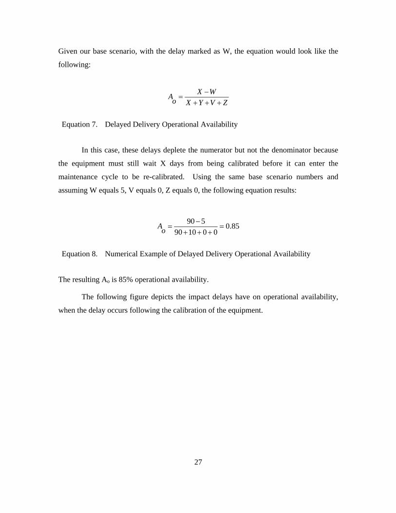
27

Given our base scenario, with the delay marked as W, the equation would look like the

following:

X WAo X Y V Z−

=+ + +

Equation 7. Delayed Delivery Operational Availability

In this case, these delays deplete the numerator but not the denominator because

the equipment must still wait X days from being calibrated before it can enter the

maintenance cycle to be re-calibrated. Using the same base scenario numbers and

assuming W equals 5, V equals 0, Z equals 0, the following equation results:

90 5 0.8590 10 0 0

Ao−

= =+ + +

Equation 8. Numerical Example of Delayed Delivery Operational Availability

The resulting Ao is 85% operational availability.

The following figure depicts the impact delays have on operational availability,

when the delay occurs following the calibration of the equipment.

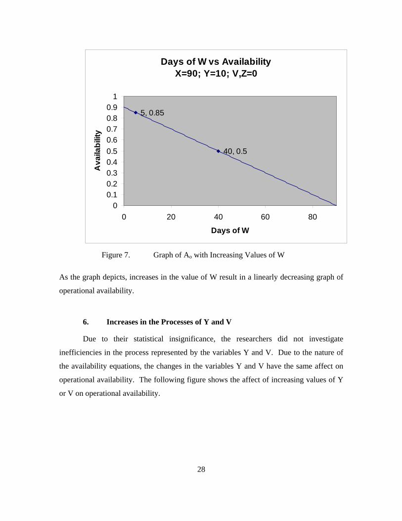
28

Days of W vs AvailabilityX=90; Y=10; V,Z=0

40, 0.5

5, 0.85

00.10.20.30.40.50.60.70.80.9

1

0 20 40 60 80

Days of W

Ava

ilabi

lity

Figure 7. Graph of Ao with Increasing Values of W

As the graph depicts, increases in the value of W result in a linearly decreasing graph of

operational availability.

6. Increases in the Processes of Y and V

Due to their statistical insignificance, the researchers did not investigate

inefficiencies in the process represented by the variables Y and V. Due to the nature of

the availability equations, the changes in the variables Y and V have the same affect on

operational availability. The following figure shows the affect of increasing values of Y

or V on operational availability.

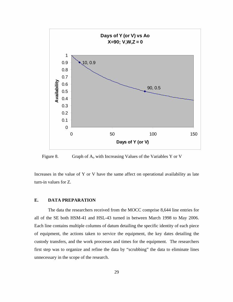
29

Days of Y (or V) vs AoX=90; V,W,Z = 0

90, 0.5

10, 0.9

00.10.20.30.40.50.60.70.80.9

1

0 50 100 150

Days of Y (or V)

Ava

ilabi

lity

Figure 8. Graph of Ao with Increasing Values of the Variables Y or V

Increases in the value of Y or V have the same affect on operational availability as late

turn-in values for Z.

E. DATA PREPARATION

The data the researchers received from the MOCC comprise 8,644 line entries for

all of the SE both HSM-41 and HSL-43 turned in between March 1998 to May 2006.

Each line contains multiple columns of datum detailing the specific identity of each piece

of equipment, the actions taken to service the equipment, the key dates detailing the

custody transfers, and the work processes and times for the equipment. The researchers

first step was to organize and refine the data by “scrubbing” the data to eliminate lines

unnecessary in the scope of the research.

30

1. Scrubbing and Sorting the MEASURE Data

As previously stated, the data comprised the 8,644 records input into the

MEASURE system for HSM-41 and HSL-43 from March 1998 to May 2006. The

researchers used the below processes to eliminate extraneous lines from the unrefined

data.

a. Eliminating Administrative Lines

As mentioned, the data contained administrative entries. These entries

reflected administrative changes in the MEASURE system, but represented no actual

work performance on equipment. An example of such an administrative entry might be

the change in the nomenclature of a tool. Such a change would result in an

administrative entry into MEASURE for every serial number of the affected tool in the

system. Through consulting with the MOCC personnel, the researchers identified these

cases when the calibrating facility spent no hours calibrating, repairing, or modifying the

equipment. The researchers identified 5,210 such lines of data and eliminated them from

the database. The net total lines of data decreased from 8,644 to 3,434.

b. Sorting the Data

The researchers sorted the 3,434 lines of data first by model (the specific

type of SE), then by equipment control number (ECN), which is specific to each serial

number of each model, and finally, in chronological order by the date the equipment

arrived (DT_RCVD) at the Calibration Laboratory/Activity.

2. Defining the Variables X, Y, V, W, and Z in the MEASURE Data

The researchers used a standard method to determine the values of X, Y, V, W,

and Z across all of the records of data. The following sub-sections outline how the

researchers calculated the values of these variables.

a. The Value of X

The researchers determined the value of X by subtracting the date the item

was due for calibration in the previous cycle from the date the artisan completed working

on the SE in the current cycle (DT_NXTDUE[of previous cycle] - DT_CMPL). The

31

researchers used this method of determining X because it provided a precise number of

days and thus greater accuracy versus multiplying the METR cycle value by 30 days.

Using this process, a 6-month METR cycle equals anywhere from 178 to 184 days long,

depending on which months the cycle spans. Additionally, some SE received a special

calibration that is longer or shorter than the METR cycle. This method correctly

calculates these non-typical METR lengths.

b. The Value of Y

The researchers determined the value of Y by subtracting the difference

between the date the artisan inducted the equipment into maintenance cycle and the date

an artisan competed calibration on the equipment (DT_CMPL - DT_INDUCT). The

result equaled the number of days an artisan worked on the SE, or more accurately, the

number of days the artisan had possession of the equipment. As a reminder, the

researchers assumed there was no wasted time between when an artisan inducted the SE

into maintenance and when he completed the maintenance. For example, if an artisan

inducted a tool on 4 March 2005 and completed working on the tool on 18 March 2005,

Y is 14 days of value added time.

c. The Value of V

The researchers determined the value of V by calculating the number of

days the calibration facility needed to induct the SE into maintenance following its arrival

at the facility, plus the estimated number of days 67A needed to transfer the SE from the

using unit to the facility. Once again, since there are no records tracking the amount of

time 67A requires to transfer a piece of equipment from the using unit to the Calibration

Laboratory/Activity, the researchers contacted 67A and obtained an estimated value of 1

day for this time. The researchers calculated the number of days the Calibration

Laboratory/Activity needed to induct the equipment into maintenance by subtracting the

difference between the date the Calibration Laboratory/Activity inducted the equipment

into MEASURE and the date the Calibration Laboratory/Activity received the equipment,

plus 1 day for transfer by 67A (DT_INDUCT - DT_RCVD + 1).

32

d. The Value of W

The researchers determined the value of W using the number of days the

equipment needed to exit the Calibration Laboratory/Activity following completion of all

work, and adding that value to the estimated number of days 67A needed to transfer the

equipment to the using unit. Once again, since there are no records tracking the amount

of time 67A needs to transfer SE from the Calibration Laboratory/Activity to the using

unit, the researchers contacted 67A and obtained an estimated value of 1 day for this

time. The researchers calculated the number of days equipment needed to leave the

Calibration Laboratory/Activity by subtracting the difference between the date the

Calibration Laboratory/Activity processed the equipment into MEASURE and the date

the artisan completed work on the equipment, plus 1 day for the transfer by 67A

(DT_PROCSD - DT_CMPL +1).

e. The Value of Z

The value of Z can be either the number of days SE departs the using unit

for the Calibration Laboratory/Activity before the expiration of the METR cycle or it can

be the number of days equipment departs the using unit after the expiration of the METR

cycle. In both cases, the researchers determined Z in the same manner. As previously

stated, the researchers organized the MEASURE entries first by part number, then by

ECN, and then chronologically by the date the Calibration Laboratory/Activity received

the asset (DT_RCVD). The researchers looked for repeating ECNs within a part number

and then calculated Z by subtracting the date of the end of the previous METR cycle, plus

one day for 67A transport, from the date the calibration facility received the asset

(DT_RCVD - (DT_NXT_DUE[of previous cycle] + 1)). The result was the value of Z

for that record, specifically, the value Z for that ECN in that specific calibration cycle. If

Z was zero, the researchers estimated that the using unit submitted the equipment into the

calibration cycle on-schedule. If Z was negative, the researchers estimated that the using

unit turned in the equipment “Z” days early. If Z was positive, the researchers estimated

the using unit turned in the equipment “Z” days late.

33

3. Filtering the Data

After the researchers organized the data and assigned formulas to calculate the

variables X, Y, Z, V, and W, the researcher’s determined the need to “filter” the data. In

this project, the term “filter” means the researchers left these records in the data series,

but they did not calculate the variable values for these records. The researchers retained

these records to maintain continuity in data and ensure they calculated the variables X

and Z correctly, since the formulas for X and Z refer to two sequential data records. As a

whole, the researchers filtered records that did not follow the typical calibration process,

or did not result in the return of equipment back to the using unit. The following sub-

sections describe the categories the researchers filtered.

a. Focusing on the North Island Calibration Laboratories/Activities (NIQ and SDB)

Multiple Calibration Laboratories/Activities performed work for HSM-41

and HSL-43 during the period of observation. The researchers focused solely the

Calibration Laboratories/Activities at NAS North Island. Examples of other facilities

include the calibration shops on-board deployed aircraft carriers or located at foreign base

facilities. The researchers filtered out all records where the facilities at North Island (in

MEASURE: NIQ or SDB) did not perform the calibration service.

b. Filtering the Equipment Condition Category

The researchers used the Equipment Condition category to determine the

condition of the equipment when it arrived at the Calibration Laboratory/Facility.

According to the MEASURE manual, the category includes the following four entries.

(1) “1” Entries. The MEASURE manual defines entries of “1”

in this category as SE that arrived to the Calibration Laboratory/Activity while still

performing within the calibration standards. (DoN, OPNAV OP43P6B, n.d.)


in this category as SE that the Calibration Laboratory/Activity serviced because, upon

arrival, the equipment did not perform within the standards of calibration. (DoN, OPNAV

OP43P6B, n.d.) In these records, the Calibration Laboratory/Activity serviced the

34

equipment and returned it to the using unit calibrated, with a new METR cycle. Initially,

the researchers debated whether or not to include these specific entries in the overall data.

The researchers used a 2-sample t-test to determine if these entries were a sub-sample of

the original dataset population. The resulting value was a 2.57% chance “Equipment

Condition 2” records came from the same population as the “Equipment Condition 1”

records. For this reason, the researchers determined not to include the “Equipment

Condition 2” records in the final data. The researchers theorized that the sub-custodians

recognized the malfunctions in the “Equipment Condition 2” records and did not treat

them the same as the “Equipment Condition 1” records. As a result, the researchers

filtered the “Equipment Condition 2” records.


in this category as SE that the Calibration Laboratory/Activity received in an inoperative

status. (DoN, OPNAV OP43P6B, n.d.) The researchers filtered these records because

they required non-routine maintenance and deviated from the standard calibration

process.


in this category as SE that the Calibration Laboratory/Activity received physically

damaged. (DoN, OPNAV OP43P6B, n.d.) The researchers filtered these items because

they required non-routine maintenance and deviated from the standard calibration

process.

c. Filtering the Service Label Category

The researchers used the MEASURE category “Service Label” to identify

typical calibrations from non-typical calibration service. The Service Label category

includes the following seven possible entries.

(1) Blank Entries. The MEASURE manual, OPNAV

OP43P6B, does not define the meaning of blank entries in the Service Label category.

The researchers left these records in for continuity in tracking individual serial numbers,

but the researchers filtered these records from the final variable values because the

purpose of these entries was indeterminate.

35


in the Service Label category as SE upon which the Calibration Activity/Laboratory

performed a standard calibration. (DoN, OPNAV OP43P6B, n.d.) The researchers

included these entries.


in the Service Label category as SE upon which the Calibration Activity/Laboratory

performed a special calibration. (DoN, OPNAV OP43P6B, n.d.) The researchers

included these entries.


in the Service Label category as SE that the Calibration Activity/Laboratory rejected back

to the using unit un-calibrated. (DoN, OPNAV OP43P6B, n.d.) The researchers filtered

the Service Label entry “3” records because these equipments deviated from the standard

calibration cycle for repairs.


in the Service Label category as SE that required no calibration action from the

Calibration Activity/Laboratory. (DoN, OPNAV OP43P6B, n.d.) The researchers filtered

the Service Label “4” records because the Calibration Activity/Laboratory did not assign

a value in the “date next due” category.


in the Service Label category as SE that the Calibration Activity/Laboratory placed in an

inactive status. (DoN, OPNAV OP43P6B, n.d.) The using unit can no longer use these

equipments until the facility performs a re-calibration on them. The researchers filtered

the Service Label “5” records because these equipments deviated from the standard

calibration cycle.


in the Service Label category as assets upon which the Calibration Activity/Laboratory

repaired the asset without performing calibration procedures. (DoN, OPNAV OP43P6B,

n.d.) These actions performed by the Calibration Activity/Laboratory do not alter any

36

existing cal dates or labels on the equipment. The researchers filtered the Service Label

“6” records because they had no affect on the current calibration cycle.

d. Filtering the Work Performed On-Site Category

The category “Work Performed On-Site” delineates whether or not the

Calibration Laboratory/Activity performed service on the SE at the using unit’s location,

or at the laboratory’s facility. Entries of “N” indicate work the laboratory completed at

their facility. Entries of “Y” indicate work the laboratory completed at the using unit.

The researchers filtered the Work Performed On-Site “Y” records because they had no

affect on the current calibration cycle.

e. Filtering of Equipment Status

The researchers used the MEASURE category “Equipment Status” to

identify how Calibration Activity/Laboratory returned the SE to the using unit. The

Label Service category includes the following three possible entries.

(1) “Blank” Entries. Blank entries in the Equipment Status

category represent SE that the Calibration Activity/Laboratory returned to the using unit

calibrated. The researchers included these entries.


in Equipment Status as SE upon which the Calibration Activity/Laboratory deemed too

expensive to repair. The researchers filtered the Equipment Status “1” records because

these equipments exited the standard calibration cycle.


in Equipment Status as SE that the Calibration Activity/Laboratory returned to the using

unit un-calibrated. The researchers filtered the Equipment Status “2” records because

these equipments exited the standard calibration cycle.

f. Filtering Calculated Values of the Metrology Cycle

The researchers filtered all records where the metrology cycle was less

than 61 days. This criterion excluded all records where the metrology cycle was a

37

negative number due to data entry errors in MEASURE. Additionally, the criterion

excluded records that were assigned a metrology cycle that was abnormally small and out

of the regular calibration cycle.

F. APPLYING THE SCENARIOS TO THE DATA

The researchers utilized two methods to analyze the data. In the first method, the

researcher’s analyzed the data as a whole. The researcher’s analysis of the entire data set

provided the overall process trends and average operational availability. First, the

researchers calculated the variable values (X, Y, Z, V, W) for each record. Next, the

researchers determined an average value of each variable for both early and late turn-ins.

Finally, the researchers calculated the Ai, the Operational Availability without Z and the

Operational Availability with Z. The results show the trends for the process

inefficiencies as a whole, but do not identify the impact on specific SE. In the second

method, the researchers identified the impact on specific SE. First, HSM-41 and HSL-43

identified their 20 most frequently utilized tools and their 10 tools that require the most

repeated repairs. The researchers used this information to focus their analysis on these

equipments to find the impact of process inefficiencies on operational availability.

The researchers listed the methods they used to calculate the availability

reductions in the following sub-sections.

1. Inefficiencies from Early Turn-ins

The researchers defined inefficiencies from early turn-ins as the reduced

availability due to the sub-custodian submitting the SE for calibration before the required

date next due. The researchers determined that early turn-ins have an affect on

operational availability, calibration manpower hours, and equipment value.

a. Reduced Operational Availability

The researchers defined reduced Operational Availability as the

percentage of time the tool is not available for use by the sub-custodian because of

process inefficiencies versus if those inefficiencies did not exist. To verify the reductions

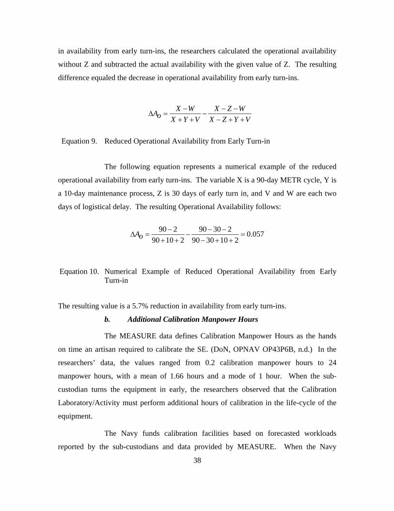
38

in availability from early turn-ins, the researchers calculated the operational availability

without Z and subtracted the actual availability with the given value of Z. The resulting

difference equaled the decrease in operational availability from early turn-ins.

X W X Z WAo X Y V X Z Y V− − −

∆ = −+ + − + +

Equation 9. Reduced Operational Availability from Early Turn-in

The following equation represents a numerical example of the reduced

operational availability from early turn-ins. The variable X is a 90-day METR cycle, Y is

a 10-day maintenance process, Z is 30 days of early turn in, and V and W are each two

days of logistical delay. The resulting Operational Availability follows:

90 2 90 30 2 0.057

90 10 2 90 30 10 2Ao

− − −∆ = − =

+ + − + +

Equation 10. Numerical Example of Reduced Operational Availability from Early Turn-in

The resulting value is a 5.7% reduction in availability from early turn-ins.

b. Additional Calibration Manpower Hours

The MEASURE data defines Calibration Manpower Hours as the hands

on time an artisan required to calibrate the SE. (DoN, OPNAV OP43P6B, n.d.) In the

researchers’ data, the values ranged from 0.2 calibration manpower hours to 24

manpower hours, with a mean of 1.66 hours and a mode of 1 hour. When the sub-

custodian turns the equipment in early, the researchers observed that the Calibration

Laboratory/Activity must perform additional hours of calibration in the life-cycle of the

equipment.

The Navy funds calibration facilities based on forecasted workloads

reported by the sub-custodians and data provided by MEASURE. When the Navy

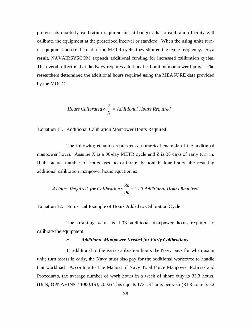
39

projects its quarterly calibration requirements, it budgets that a calibration facility will

calibrate the equipment at the prescribed interval or standard. When the using units turn-

in equipment before the end of the METR cycle, they shorten the cycle frequency. As a

result, NAVAIRSYSCOM expends additional funding for increased calibration cycles.

The overall effect is that the Navy requires additional calibration manpower hours. The

researchers determined the additional hours required using the MEASURE data provided

by the MOCC.

ZHours Calibrated× = Additional Hours RequiredX

Equation 11. Additional Calibration Manpower Hours Required

The following equation represents a numerical example of the additional

manpower hours. Assume X is a 90-day METR cycle and Z is 30 days of early turn in.

If the actual number of hours used to calibrate the tool is four hours, the resulting

additional calibration manpower hours equation is:

304 Hours Required for Calibration× = 1.33 Additional Hours Required90

Equation 12. Numerical Example of Hours Added to Calibration Cycle

The resulting value is 1.33 additional manpower hours required to

calibrate the equipment.

c. Additional Manpower Needed for Early Calibrations

In additional to the extra calibration hours the Navy pays for when using

units turn assets in early, the Navy must also pay for the additional workforce to handle

that workload. According to The Manual of Navy Total Force Manpower Policies and

Procedures, the average number of work hours in a week of shore duty is 33.3 hours.

(DoN, OPNAVINST 1000.16J, 2002) This equals 1731.6 hours per year (33.3 hours x 52

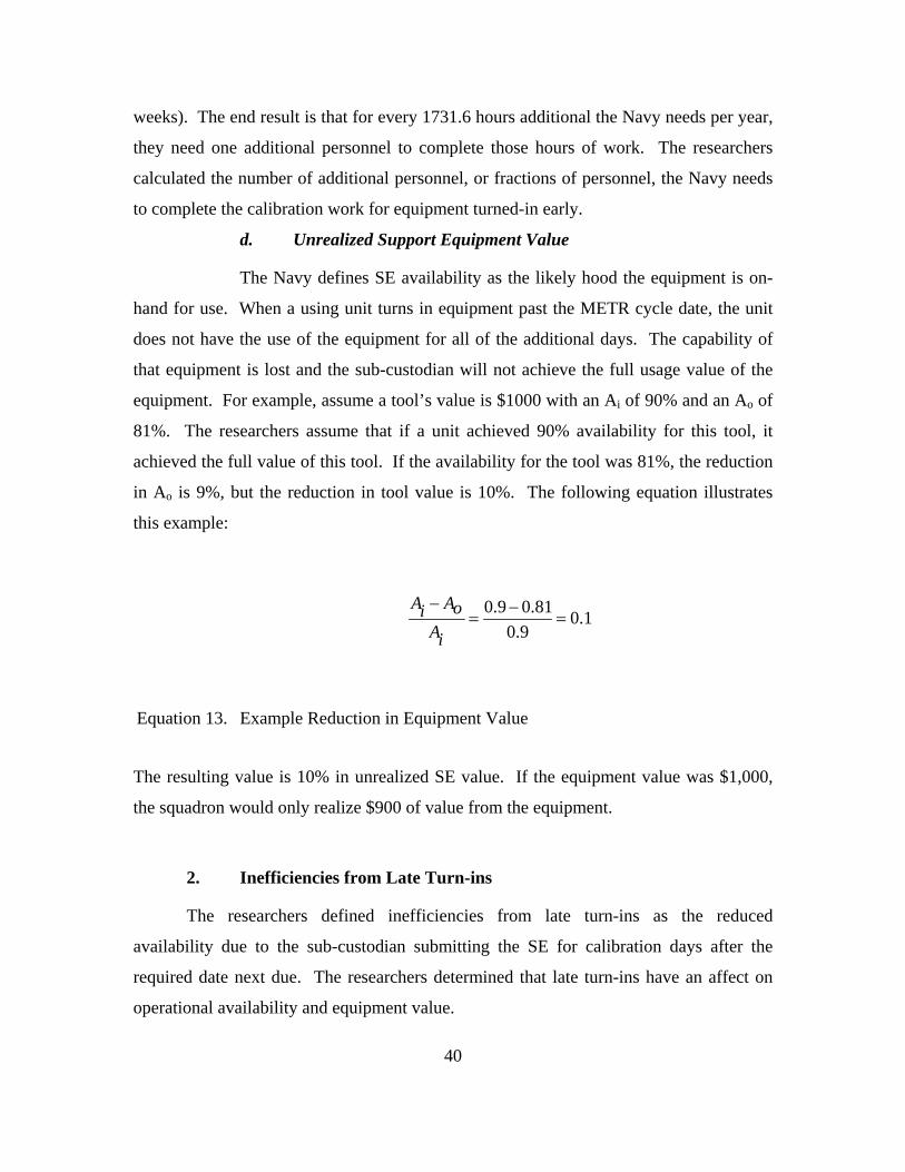
40

weeks). The end result is that for every 1731.6 hours additional the Navy needs per year,

they need one additional personnel to complete those hours of work. The researchers

calculated the number of additional personnel, or fractions of personnel, the Navy needs

to complete the calibration work for equipment turned-in early.

d. Unrealized Support Equipment Value

The Navy defines SE availability as the likely hood the equipment is on-

hand for use. When a using unit turns in equipment past the METR cycle date, the unit

does not have the use of the equipment for all of the additional days. The capability of

that equipment is lost and the sub-custodian will not achieve the full usage value of the

equipment. For example, assume a tool’s value is $1000 with an Ai of 90% and an Ao of

81%. The researchers assume that if a unit achieved 90% availability for this tool, it

achieved the full value of this tool. If the availability for the tool was 81%, the reduction

in Ao is 9%, but the reduction in tool value is 10%. The following equation illustrates

this example:

0.9 0.81 0.10.9

A AoiAi

− −= =

Equation 13. Example Reduction in Equipment Value

The resulting value is 10% in unrealized SE value. If the equipment value was $1,000,

the squadron would only realize $900 of value from the equipment.

2. Inefficiencies from Late Turn-ins

The researchers defined inefficiencies from late turn-ins as the reduced

availability due to the sub-custodian submitting the SE for calibration days after the

required date next due. The researchers determined that late turn-ins have an affect on

operational availability and equipment value.

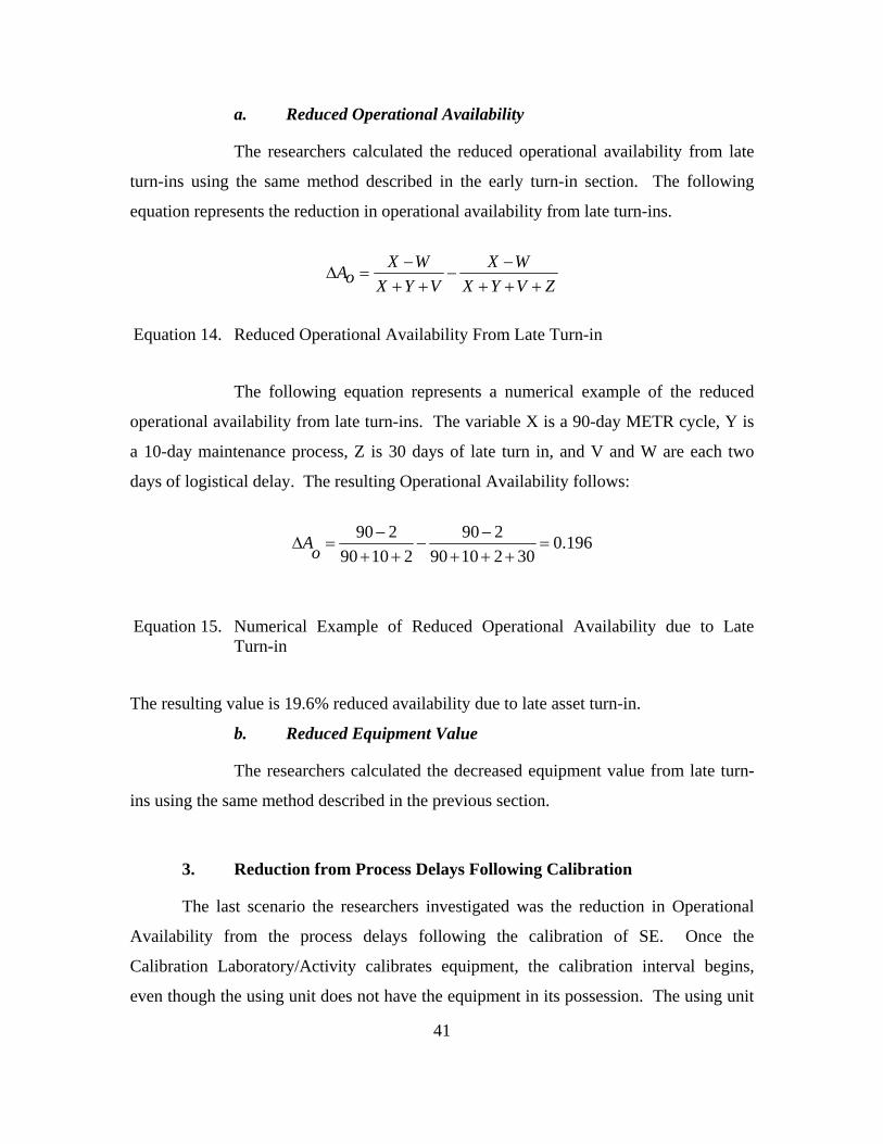
41

a. Reduced Operational Availability

The researchers calculated the reduced operational availability from late

turn-ins using the same method described in the early turn-in section. The following

equation represents the reduction in operational availability from late turn-ins.

X W X WAo X Y V X Y V Z− −

∆ = −+ + + + +

Equation 14. Reduced Operational Availability From Late Turn-in

The following equation represents a numerical example of the reduced

operational availability from late turn-ins. The variable X is a 90-day METR cycle, Y is

a 10-day maintenance process, Z is 30 days of late turn in, and V and W are each two

days of logistical delay. The resulting Operational Availability follows:

90 2 90 2 0.196

90 10 2 90 10 2 30Ao

− −∆ = − =

+ + + + +

Equation 15. Numerical Example of Reduced Operational Availability due to Late Turn-in

The resulting value is 19.6% reduced availability due to late asset turn-in.

b. Reduced Equipment Value

The researchers calculated the decreased equipment value from late turn-

ins using the same method described in the previous section.

3. Reduction from Process Delays Following Calibration

The last scenario the researchers investigated was the reduction in Operational

Availability from the process delays following the calibration of SE. Once the

Calibration Laboratory/Activity calibrates equipment, the calibration interval begins,

even though the using unit does not have the equipment in its possession. The using unit

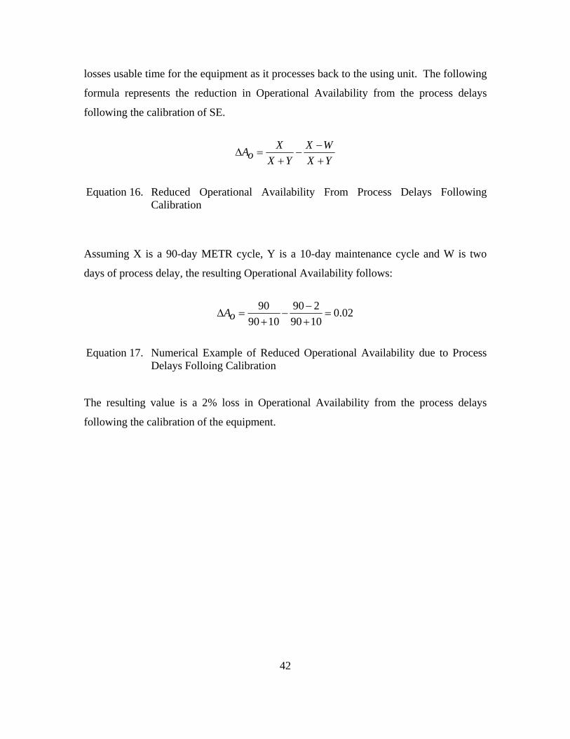
42

losses usable time for the equipment as it processes back to the using unit. The following

formula represents the reduction in Operational Availability from the process delays

following the calibration of SE.

X X WAo X Y X Y

−∆ = −

+ +

Equation 16. Reduced Operational Availability From Process Delays Following Calibration

Assuming X is a 90-day METR cycle, Y is a 10-day maintenance cycle and W is two

days of process delay, the resulting Operational Availability follows:

90 90 2 0.02

90 10 90 10Ao

−∆ = − =

+ +

Equation 17. Numerical Example of Reduced Operational Availability due to Process Delays Folloing Calibration

The resulting value is a 2% loss in Operational Availability from the process delays

following the calibration of the equipment.

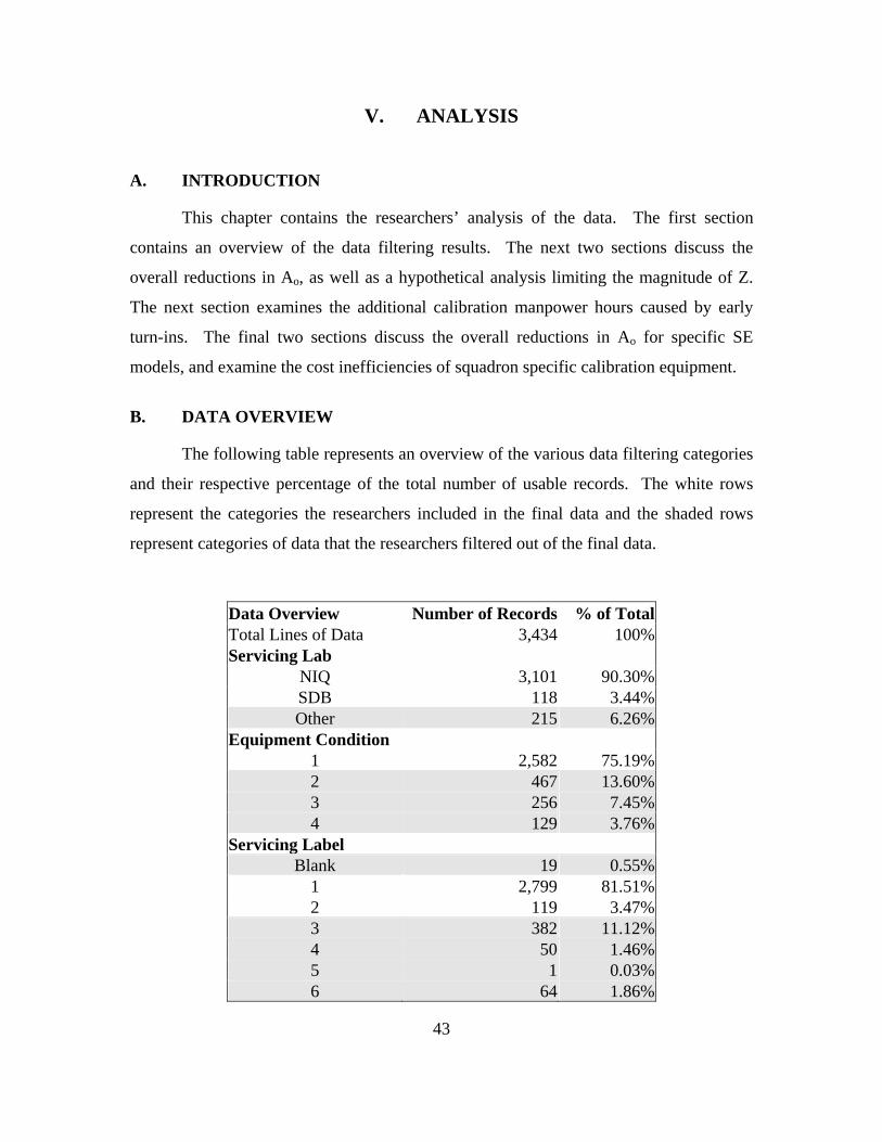
43

V. ANALYSIS

A. INTRODUCTION

This chapter contains the researchers’ analysis of the data. The first section

contains an overview of the data filtering results. The next two sections discuss the

overall reductions in Ao, as well as a hypothetical analysis limiting the magnitude of Z.

The next section examines the additional calibration manpower hours caused by early

turn-ins. The final two sections discuss the overall reductions in Ao for specific SE

models, and examine the cost inefficiencies of squadron specific calibration equipment.

B. DATA OVERVIEW

The following table represents an overview of the various data filtering categories

and their respective percentage of the total number of usable records. The white rows

represent the categories the researchers included in the final data and the shaded rows

represent categories of data that the researchers filtered out of the final data.

Data Overview Number of Records % of Total Total Lines of Data 3,434 100% Servicing Lab

NIQ 3,101 90.30% SDB 118 3.44% Other 215 6.26%

Equipment Condition 1 2,582 75.19% 2 467 13.60% 3 256 7.45% 4 129 3.76%

Servicing Label Blank 19 0.55%

1 2,799 81.51% 2 119 3.47% 3 382 11.12% 4 50 1.46% 5 1 0.03% 6 64 1.86%

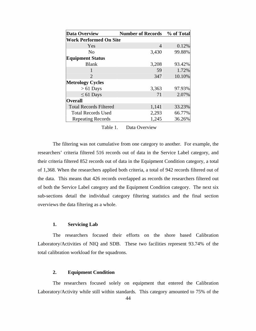
44

Data Overview Number of Records % of Total Work Performed On Site

Yes 4 0.12% No 3,430 99.88%

Equipment Status Blank 3,208 93.42%

1 59 1.72% 2 347 10.10%

Metrology Cycles > 61 Days 3,363 97.93% ≤ 61 Days 71 2.07%

Overall Total Records Filtered 1,141 33.23%

Total Records Used 2,293 66.77% Repeating Records 1,245 36.26%

Table 1. Data Overview

The filtering was not cumulative from one category to another. For example, the

researchers’ criteria filtered 516 records out of data in the Service Label category, and

their criteria filtered 852 records out of data in the Equipment Condition category, a total

of 1,368. When the researchers applied both criteria, a total of 942 records filtered out of

the data. This means that 426 records overlapped as records the researchers filtered out

of both the Service Label category and the Equipment Condition category. The next six

sub-sections detail the individual category filtering statistics and the final section

overviews the data filtering as a whole.

1. Servicing Lab

The researchers focused their efforts on the shore based Calibration

Laboratory/Activities of NIQ and SDB. These two facilities represent 93.74% of the

total calibration workload for the squadrons.

2. Equipment Condition

The researchers focused solely on equipment that entered the Calibration

Laboratory/Activity while still within standards. This category amounted to 75% of the

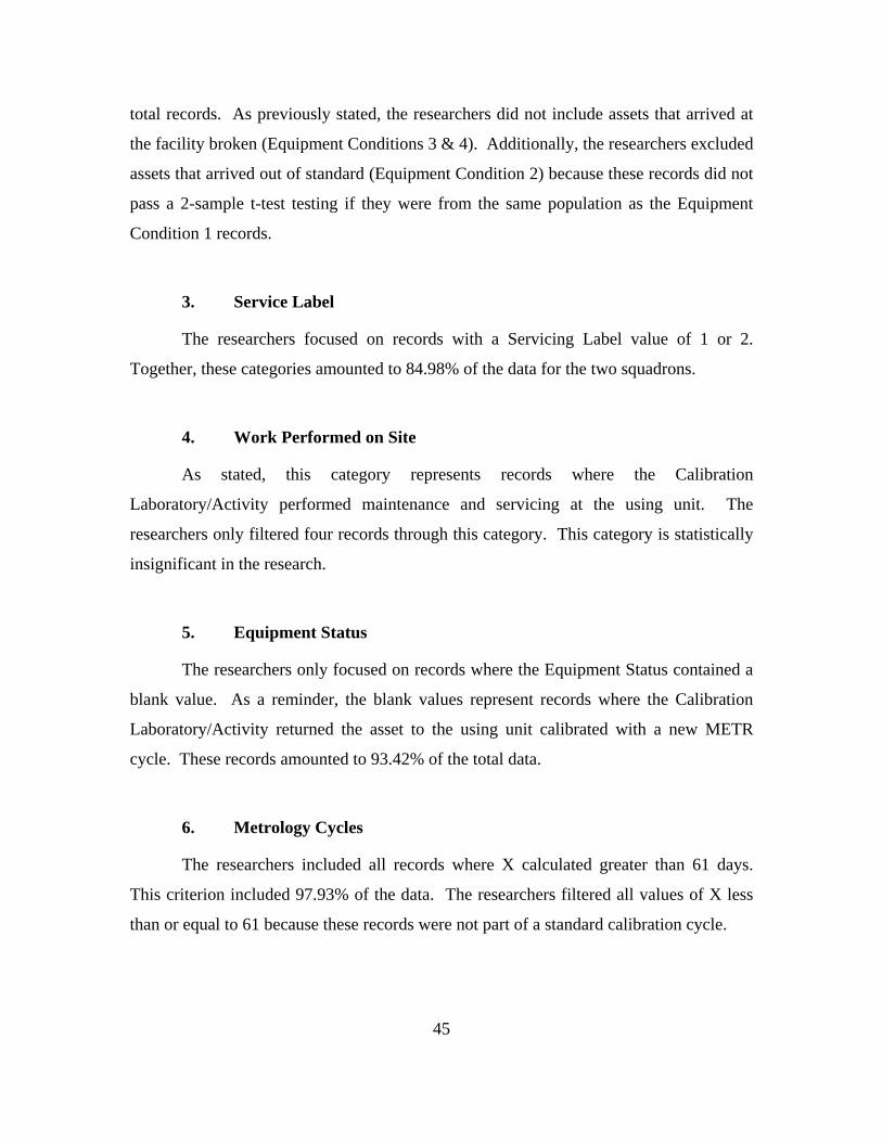
45

total records. As previously stated, the researchers did not include assets that arrived at

the facility broken (Equipment Conditions 3 & 4). Additionally, the researchers excluded

assets that arrived out of standard (Equipment Condition 2) because these records did not

pass a 2-sample t-test testing if they were from the same population as the Equipment

Condition 1 records.

3. Service Label

The researchers focused on records with a Servicing Label value of 1 or 2.

Together, these categories amounted to 84.98% of the data for the two squadrons.

4. Work Performed on Site

As stated, this category represents records where the Calibration

Laboratory/Activity performed maintenance and servicing at the using unit. The

researchers only filtered four records through this category. This category is statistically

insignificant in the research.

5. Equipment Status

The researchers only focused on records where the Equipment Status contained a

blank value. As a reminder, the blank values represent records where the Calibration

Laboratory/Activity returned the asset to the using unit calibrated with a new METR

cycle. These records amounted to 93.42% of the total data.

6. Metrology Cycles

The researchers included all records where X calculated greater than 61 days.

This criterion included 97.93% of the data. The researchers filtered all values of X less

than or equal to 61 because these records were not part of a standard calibration cycle.

46

7. Summary

Overall, the researchers filtered out 33% of the data. This means that their

analysis is pertinent to 66% of the total calibration activity for these squadrons. Of this

66%, slightly more than half of these records (36.26% of the total) were repeat entries for

the same serial numbers. The researchers were able to use these records to calculate the

values of X and Z and make their recommendations.

C. OVERALL REDUCTIONS IN OPERATIONAL AVAILABILITY

Table 2 illustrates the overall Operational Availability for both of the using units

during the entire scope of the data. The table has four columns. The first column

represents early turn-ins, the second column represents late turn-ins, the third column

represents on-schedule turn-ins, and the final column is an overall analysis taking in the

proportion of each of the previous three columns.

The first section of rows in the table outline the number or records of each type of

column and lists the average value of each variable (X, Y, Z, V, W). The second section

breaks down the Ai, the Ao without Z, and the Ao with Z. For the overall average

Operational Availability, the researchers used the proportional average of the first three

rows since there is no specific formula that accounts for both positive and negative values

of Z.

Overall Operational Availability Chart

Early Turn-ins

Late Turn-ins

On-Schedule Turn-ins

Overall

Number of Records (% of total) 793 (63.6%)

426 (34.2%)

28 (2.2%)

1,247

Avg of X in days 460.83 392.52 328.86 435.1

Avg of Y in days 6.52 7.63 4.93 6.86

Avg of Z in days -153.11 30.51 0 |107.39|

Avg of V in days 3.6 3.37 2.39 3.5

Avg of W in days 3.96 3.31 3.79 3.74

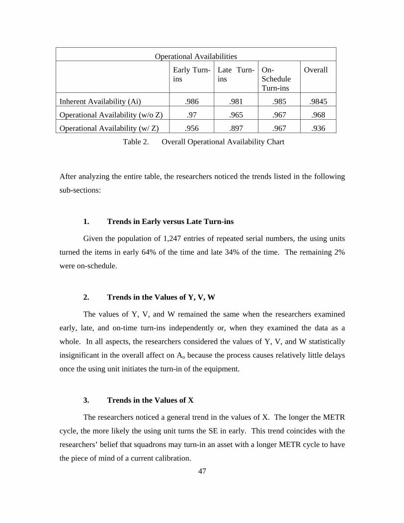
47

Operational Availabilities

Early Turn-ins

Late Turn-ins

On-Schedule Turn-ins

Overall

Inherent Availability (Ai) .986 .981 .985 .9845

Operational Availability (w/o Z) .97 .965 .967 .968

Operational Availability (w/ Z) .956 .897 .967 .936

Table 2. Overall Operational Availability Chart

After analyzing the entire table, the researchers noticed the trends listed in the following

sub-sections:

1. Trends in Early versus Late Turn-ins

Given the population of 1,247 entries of repeated serial numbers, the using units

turned the items in early 64% of the time and late 34% of the time. The remaining 2%

were on-schedule.

2. Trends in the Values of Y, V, W

The values of Y, V, and W remained the same when the researchers examined

early, late, and on-time turn-ins independently or, when they examined the data as a

whole. In all aspects, the researchers considered the values of Y, V, and W statistically

insignificant in the overall affect on Ao because the process causes relatively little delays

once the using unit initiates the turn-in of the equipment.

3. Trends in the Values of X

The researchers noticed a general trend in the values of X. The longer the METR

cycle, the more likely the using unit turns the SE in early. This trend coincides with the

researchers’ belief that squadrons may turn-in an asset with a longer METR cycle to have

the piece of mind of a current calibration.

48

4. Trends in the Values of Z

The researchers noticed a distinctive trend in the values of Z in that the magnitude

of Z in the early turn-ins is much greater than the magnitude in the late turn-ins.

5. Trends in Ai and Ao

To begin, the researchers calculated the Ai for early, late, and on-tine turn-ins.

They observed that all three scenarios had high availabilities due to the relative

magnitudes of X and Y. When the researchers calculated the Aos without Z, a slight,

uniform reduction occurred across all three scenarios. When the researchers included the

variable Z, they noted that the effects of Z on the late turn-ins were more substantial than

the effects on the early turn-ins. The researchers determined that the best way to increase

the Ao through process change was to limit the magnitude of Z.

D. HYPOTHETICAL ANALYSIS

The researchers recognized two facts after analyzing the data. First, the largest

source of inefficiency lays in the using units variable turn-in trends for SE. After the

units turn-in equipment, the process is relatively efficient. When compared to the

magnitudes of X or Z, the magnitudes of V, W, and Y are relatively small. The second

realization is that the Navy cannot expect every unit to turn in every asset on the day the

meter cycle expires. Instead, the Navy needs some sort of common sense approach to

reduce the variability in turn-in, but allow a reasonable window.

The researchers considered an approach by modeling three scenarios where Z is

of no greater magnitude than 7, 10, or 14 days. They recalculated the value of Z, by

limiting all values greater than 7, 10, or 14 days equal to their respective limits. The

researchers left values smaller than the limit unchanged. Appendix D lists the data for

each situation. The Ao changes little when the researchers limit the values of early turn-

ins as compared to the changes when the researchers limited the late turn-ins. The

researchers considered this fact in their final recommendations.

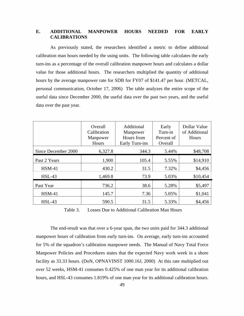
49

E. ADDITIONAL MANPOWER HOURS NEEDED FOR EARLY CALIBRATIONS

As previously stated, the researchers identified a metric to define additional

calibration man hours needed by the using units. The following table calculates the early

turn-ins as a percentage of the overall calibration manpower hours and calculates a dollar

value for those additional hours. The researchers multiplied the quantity of additional

hours by the average manpower rate for SDB for FY07 of $141.47 per hour. (METCAL,

personal communication, October 17, 2006) The table analyzes the entire scope of the

useful data since December 2000, the useful data over the past two years, and the useful

data over the past year.

Overall Calibration Manpower

Hours

Additional Manpower Hours from

Early Turn-ins

Early Turn-in

Percent of Overall

Dollar Value of Additional

Hours

Since December 2000 6,327.8 344.3 5.44% $48,708

Past 2 Years 1,900 105.4 5.55% $14,910

HSM-41 430.2 31.5 7.32% $4,456

HSL-43 1,469.8 73.9 5.03% $10,454

Past Year 736.2 38.6 5.28% $5,497

HSM-41 145.7 7.36 5.05% $1,041

HSL-43 590.5 31.5 5.33% $4,456

Table 3. Losses Due to Additional Calibration Man Hours

The end-result was that over a 6-year span, the two units paid for 344.3 additional

manpower hours of calibration from early turn-ins. On average, early turn-ins accounted

for 5% of the squadron’s calibration manpower needs. The Manual of Navy Total Force

Manpower Policies and Procedures states that the expected Navy work week in a shore

facility as 33.33 hours. (DoN, OPNAVINST 1000.16J, 2000) At this rate multiplied out

over 52 weeks, HSM-41 consumes 0.425% of one man year for its additional calibration

hours, and HSL-43 consumes 1.819% of one man year for its additional calibration hours.

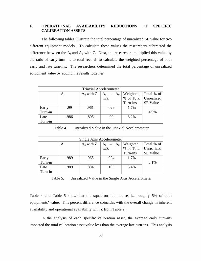
50

F. OPERATIONAL AVAILABILITY REDUCTIONS OF SPECIFIC CALIBRATION ASSETS

The following tables illustrate the total percentage of unrealized SE value for two

different equipment models. To calculate these values the researchers subtracted the

difference between the Ai and Ao with Z. Next, the researchers multiplied this value by

the ratio of early turn-ins to total records to calculate the weighted percentage of both

early and late turn-ins. The researchers determined the total percentage of unrealized

equipment value by adding the results together.

Triaxial Accelerometer Ai Ao with Z Ai – Ao

w/Z Weighted % of Total Turn-ins

Total % of Unrealized SE Value

Early Turn-in

.99 .961 .029 1.7%

Late Turn-in

.986 .895 .09 3.2%

4.9%

Table 4. Unrealized Value in the Triaxial Accelerometer

Single Axis Accelerometer

Ai Ao with Z Ai – Ao w/Z

Weighted % of Total Turn-ins

Total % of Unrealized SE Value

Early Turn-in

.989 .965 .024 1.7%

Late Turn-in

.989 .884 .105 3.4%

5.1%

Table 5. Unrealized Value in the Single Axis Accelerometer

Table 4 and Table 5 show that the squadrons do not realize roughly 5% of both

equipments’ value. This percent difference coincides with the overall change in inherent

availability and operational availability with Z from Table 2.

In the analysis of each specific calibration asset, the average early turn-ins

impacted the total calibration asset value less than the average late turn-ins. This analysis

51

supports the researchers’ previous findings. The resulting dollar values for the above

calculations show relatively insignificant amounts of calibration asset values wasted by

the squadrons. The researchers have shown, however, that when squadrons turn in

calibration assets late on average they lose a greater amount of the value of the

calibration asset.

52


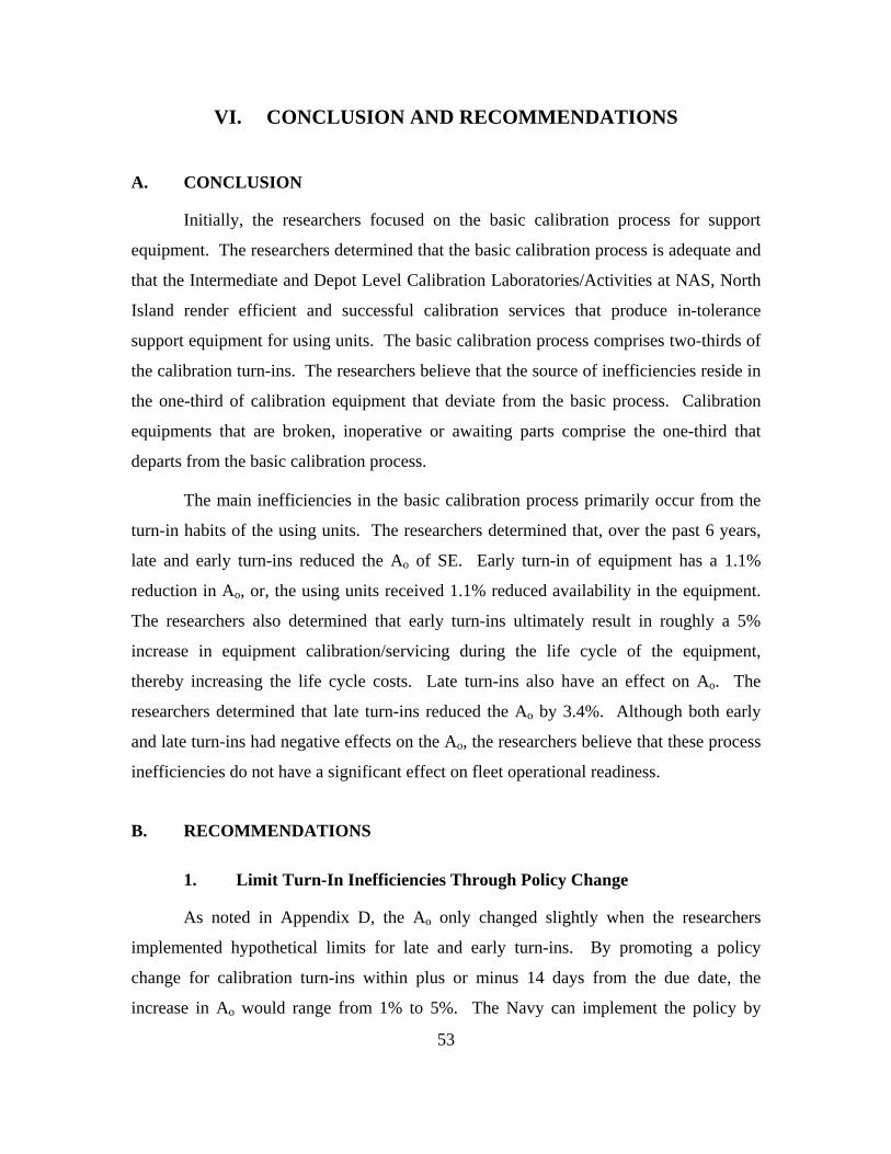
53

VI. CONCLUSION AND RECOMMENDATIONS

A. CONCLUSION

Initially, the researchers focused on the basic calibration process for support

equipment. The researchers determined that the basic calibration process is adequate and

that the Intermediate and Depot Level Calibration Laboratories/Activities at NAS, North

Island render efficient and successful calibration services that produce in-tolerance

support equipment for using units. The basic calibration process comprises two-thirds of

the calibration turn-ins. The researchers believe that the source of inefficiencies reside in

the one-third of calibration equipment that deviate from the basic process. Calibration

equipments that are broken, inoperative or awaiting parts comprise the one-third that

departs from the basic calibration process.

The main inefficiencies in the basic calibration process primarily occur from the

turn-in habits of the using units. The researchers determined that, over the past 6 years,

late and early turn-ins reduced the Ao of SE. Early turn-in of equipment has a 1.1%

reduction in Ao, or, the using units received 1.1% reduced availability in the equipment.

The researchers also determined that early turn-ins ultimately result in roughly a 5%

increase in equipment calibration/servicing during the life cycle of the equipment,

thereby increasing the life cycle costs. Late turn-ins also have an effect on Ao. The

researchers determined that late turn-ins reduced the Ao by 3.4%. Although both early

and late turn-ins had negative effects on the Ao, the researchers believe that these process

inefficiencies do not have a significant effect on fleet operational readiness.

B. RECOMMENDATIONS

1. Limit Turn-In Inefficiencies Through Policy Change

As noted in Appendix D, the Ao only changed slightly when the researchers

implemented hypothetical limits for late and early turn-ins. By promoting a policy

change for calibration turn-ins within plus or minus 14 days from the due date, the

increase in Ao would range from 1% to 5%. The Navy can implement the policy by

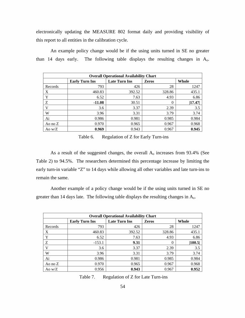
54

electronically updating the MEASURE 802 format daily and providing visibility of

this report to all entities in the calibration cycle.

An example policy change would be if the using units turned in SE no greater

than 14 days early. The following table displays the resulting changes in Ao.

Overall Operational Availability Chart Early Turn Ins Late Turn Ins Zeros Whole Records 793 426 28 1247 X 460.83 392.52 328.86 435.1 Y 6.52 7.63 4.93 6.86 Z -11.08 30.51 0 |17.47| V 3.6 3.37 2.39 3.5 W 3.96 3.31 3.79 3.74 Ai 0.986 0.981 0.985 0.984 Ao no Z 0.970 0.965 0.967 0.968 Ao w/Z 0.969 0.943 0.967 0.945

Table 6. Regulation of Z for Early Turn-ins

As a result of the suggested changes, the overall Ao increases from 93.4% (See

Table 2) to 94.5%. The researchers determined this percentage increase by limiting the

early turn-in variable “Z” to 14 days while allowing all other variables and late turn-ins to

remain the same.

Another example of a policy change would be if the using units turned in SE no

greater than 14 days late. The following table displays the resulting changes in Ao.


Table 7. Regulation of Z for Late Turn-ins

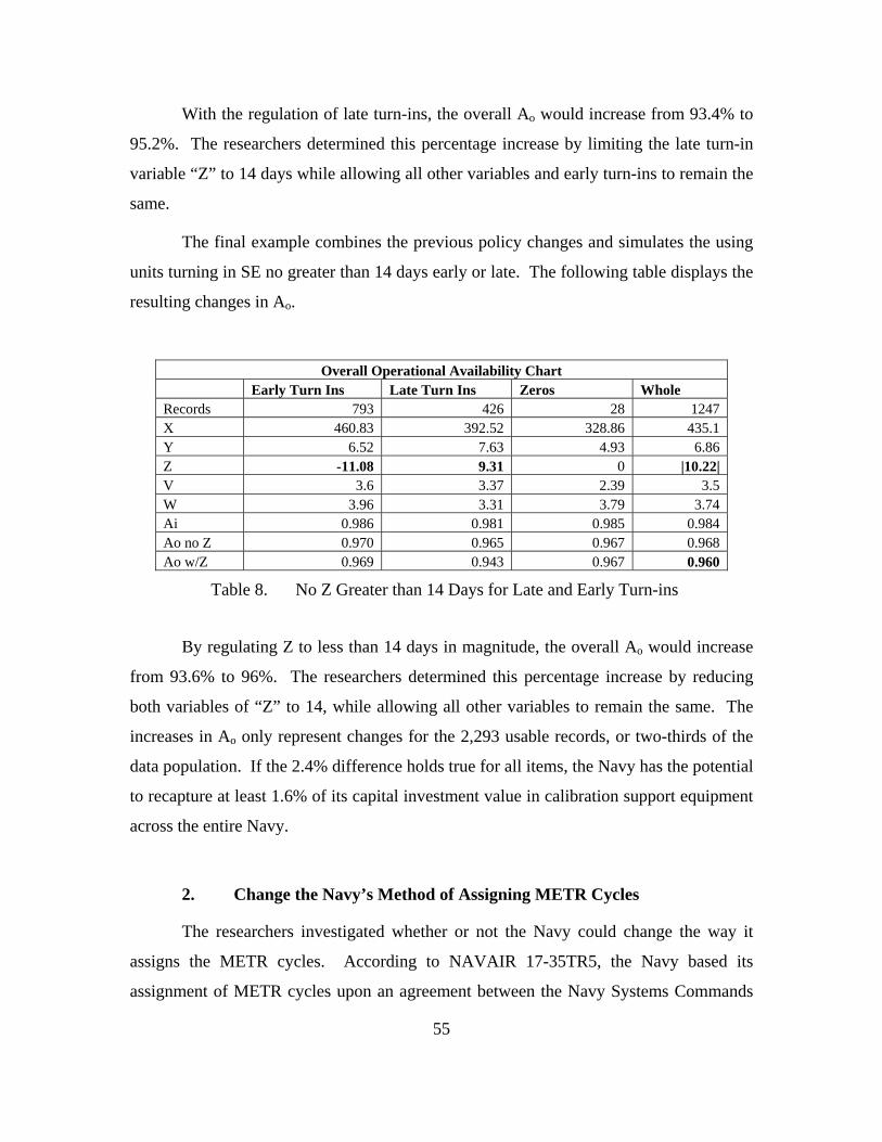
55

With the regulation of late turn-ins, the overall Ao would increase from 93.4% to

95.2%. The researchers determined this percentage increase by limiting the late turn-in

variable “Z” to 14 days while allowing all other variables and early turn-ins to remain the

same.

The final example combines the previous policy changes and simulates the using

units turning in SE no greater than 14 days early or late. The following table displays the

resulting changes in Ao.


Table 8. No Z Greater than 14 Days for Late and Early Turn-ins

By regulating Z to less than 14 days in magnitude, the overall Ao would increase

from 93.6% to 96%. The researchers determined this percentage increase by reducing

both variables of “Z” to 14, while allowing all other variables to remain the same. The

increases in Ao only represent changes for the 2,293 usable records, or two-thirds of the

data population. If the 2.4% difference holds true for all items, the Navy has the potential

to recapture at least 1.6% of its capital investment value in calibration support equipment

across the entire Navy.

2. Change the Navy’s Method of Assigning METR Cycles

The researchers investigated whether or not the Navy could change the way it

assigns the METR cycles. According to NAVAIR 17-35TR5, the Navy based its

assignment of METR cycles upon an agreement between the Navy Systems Commands

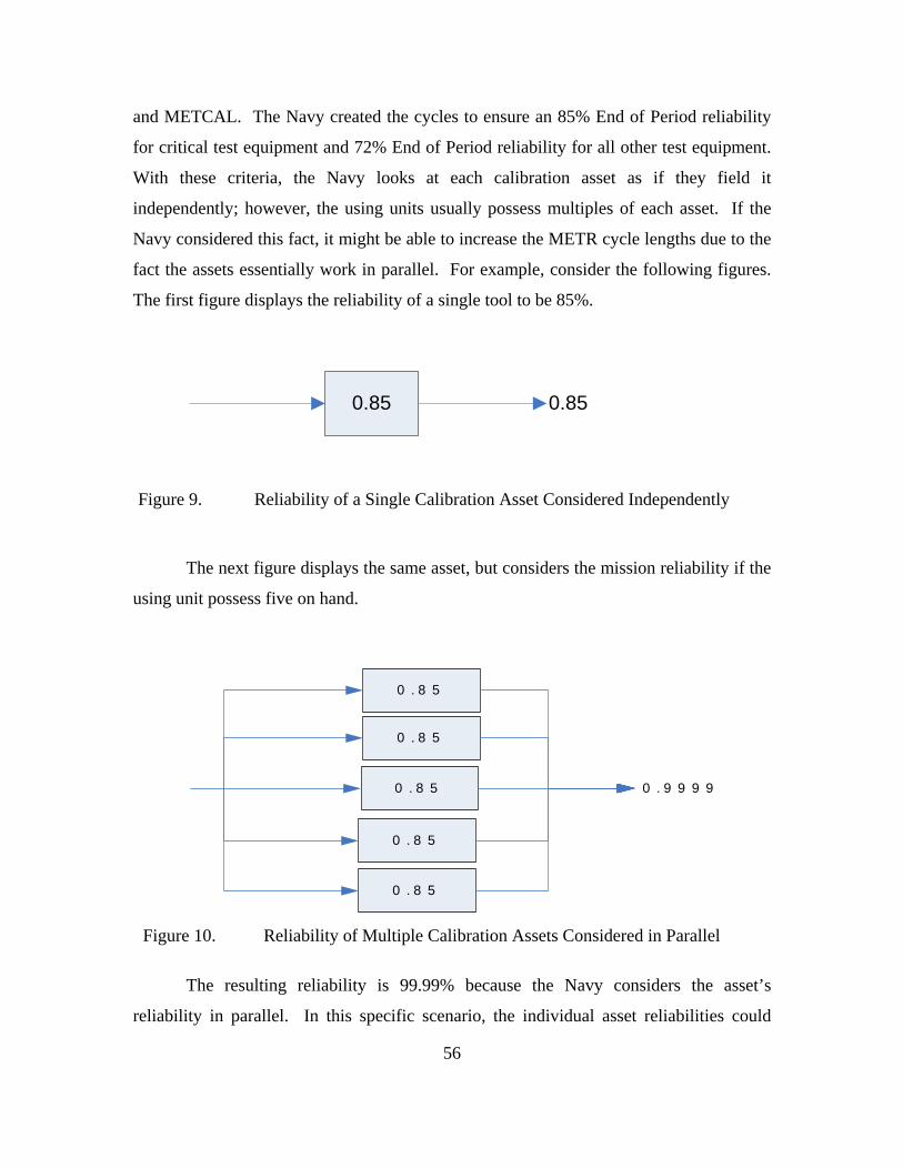
56

and METCAL. The Navy created the cycles to ensure an 85% End of Period reliability

for critical test equipment and 72% End of Period reliability for all other test equipment.

With these criteria, the Navy looks at each calibration asset as if they field it

independently; however, the using units usually possess multiples of each asset. If the

Navy considered this fact, it might be able to increase the METR cycle lengths due to the

fact the assets essentially work in parallel. For example, consider the following figures.

The first figure displays the reliability of a single tool to be 85%.

0.85 0.85

Figure 9. Reliability of a Single Calibration Asset Considered Independently

The next figure displays the same asset, but considers the mission reliability if the

using unit possess five on hand.

0 . 8 5 0 . 9 9 9 9

0 . 8 5

0 . 8 5

0 . 8 5

0 . 8 5

Figure 10. Reliability of Multiple Calibration Assets Considered in Parallel

The resulting reliability is 99.99% because the Navy considers the asset’s

reliability in parallel. In this specific scenario, the individual asset reliabilities could

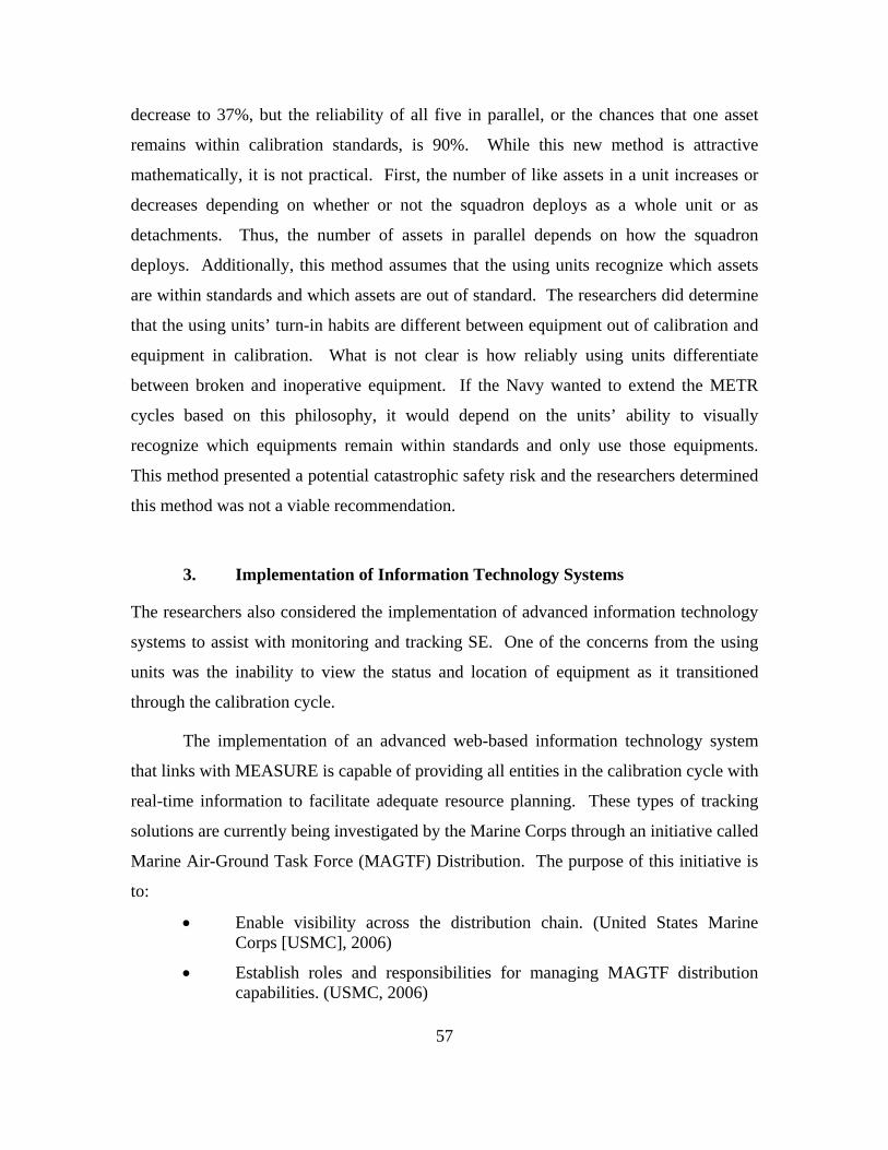
57

decrease to 37%, but the reliability of all five in parallel, or the chances that one asset

remains within calibration standards, is 90%. While this new method is attractive

mathematically, it is not practical. First, the number of like assets in a unit increases or

decreases depending on whether or not the squadron deploys as a whole unit or as

detachments. Thus, the number of assets in parallel depends on how the squadron

deploys. Additionally, this method assumes that the using units recognize which assets

are within standards and which assets are out of standard. The researchers did determine

that the using units’ turn-in habits are different between equipment out of calibration and

equipment in calibration. What is not clear is how reliably using units differentiate

between broken and inoperative equipment. If the Navy wanted to extend the METR

cycles based on this philosophy, it would depend on the units’ ability to visually

recognize which equipments remain within standards and only use those equipments.

This method presented a potential catastrophic safety risk and the researchers determined

this method was not a viable recommendation.

3. Implementation of Information Technology Systems

The researchers also considered the implementation of advanced information technology

systems to assist with monitoring and tracking SE. One of the concerns from the using

units was the inability to view the status and location of equipment as it transitioned

through the calibration cycle.

The implementation of an advanced web-based information technology system

that links with MEASURE is capable of providing all entities in the calibration cycle with

real-time information to facilitate adequate resource planning. These types of tracking

solutions are currently being investigated by the Marine Corps through an initiative called

Marine Air-Ground Task Force (MAGTF) Distribution. The purpose of this initiative is

to:

• Enable visibility across the distribution chain. (United States Marine Corps [USMC], 2006)

• Establish roles and responsibilities for managing MAGTF distribution capabilities. (USMC, 2006)

58

• Achieve centralized control of the MAGTF distribution chain. (USMC, 2006)

• Initiate and integrate people, processes, and technologies via new doctrine, organizations, training, and material solutions. (USMC, 2006)

The implementation and integration of this type of information technology system

for the calibration cycle would involve creating a new software package to capture the

data, training personnel on the new system and providing support personnel to maintain

the system. Although this option could provide total asset visibility and increased

information for planning purposes, the researchers decided that this option would be too

cost intensive to justify the returns.

C. FURTHER STUDY

Beyond the submission of recommendations, the researchers also determined that

the Navy could conduct further investigation of the following subjects to provide more

information on how to make the calibration process more efficient for increased unit

readiness.

1. Increase the Length of Metrology Intervals

OPNAV OP43P6B defines metrology intervals as the maximum interval, or

number of months, a specific item of equipment, may stay in service before it requires

calibration or servicing from a Calibration Laboratory/Activity. (DoN, OPNAV

OP43P6B, n.d.) NWSC creates and monitors these intervals with uniform and traceable

links to the NIST, U.S. Naval Observatory, or DoD approved calibration facilities. As

the researchers reviewed the MEASURE data, they noticed that out of the 3,434 lines of

data, 2,582 contained an Equipment Condition code of 1.

According to OPNAV OP43P6B, an Equipment Condition code of 1 means that

during calibration, the equipment performed to specifications without adjustments. (DoN,

OPNAV OP43P6B, n.d.) Further research on this topic would possibly save on funding

and man-power requirements, while also slightly increasing equipment Ao.

59

2. Work Center 67A

One of the difficult aspects of the research was determining the actual cycle time

of SE at Work Center 67A. As discussed in Chapter II, personnel from Work Center 67A

pick up the equipment and take it directly to the Calibration Laboratory/Activity. After

the laboratory calibrates the equipment, the 67A personnel pick up the equipment, sort it,

and return it to the using unit. Although work center managers claim the cycle time at the

facility is one day, some using unit personnel claim that some equipment remains in the

work center longer. Further research on this topic could lead to a reduction in turn-

around time and increased equipment Ao.

3. Monitor Support Equipment Throughout the Calibration Process

Currently, MEASURE tracks SE at the Calibration Laboratory/Activity. While

MEASURE is ideal for tracking equipment activity within the Calibration

Laboratory/Activity, it does not track equipment movement and activity outside of the

facility. If the Navy extended MEASURE to include all entities within the calibration

process, it could properly track turnaround time by maintaining accountability and asset

visibility.

4. Calibration Support Equipment Repair and Maintenance Process

When the researchers first interviewed using unit personnel at North Island, most

viewed the calibration process as inefficient and lengthy. Through an in-depth analysis

of the standard calibration process, the researchers determined the process to be efficient.

It is important to note that the scope of the research did not include broken or inoperable

equipment. Further research may determine that the frustrations of using units may lie in

the repair and maintenance aspects of the calibration processes, and the ages of the SE.

60


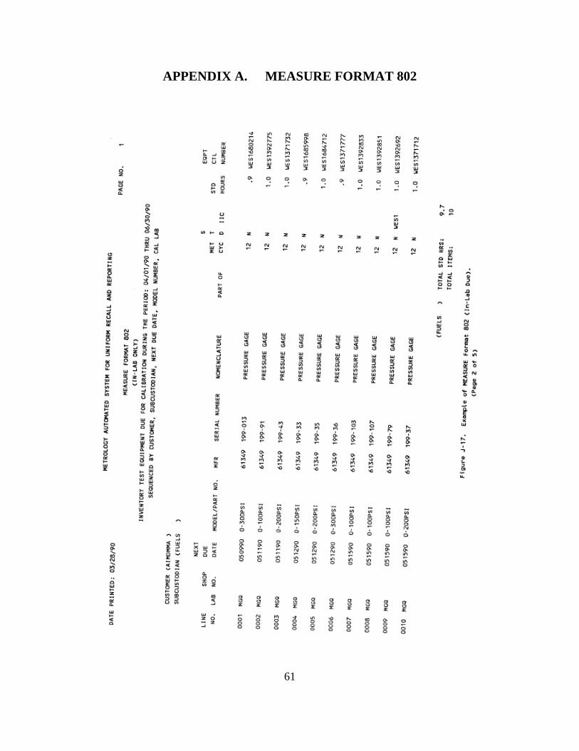
61

APPENDIX A. MEASURE FORMAT 802

62


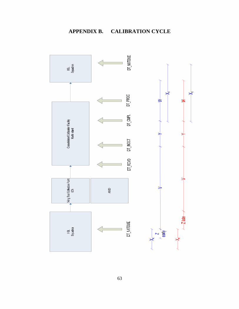
63

APPENDIX B. CALIBRATION CYCLE

64


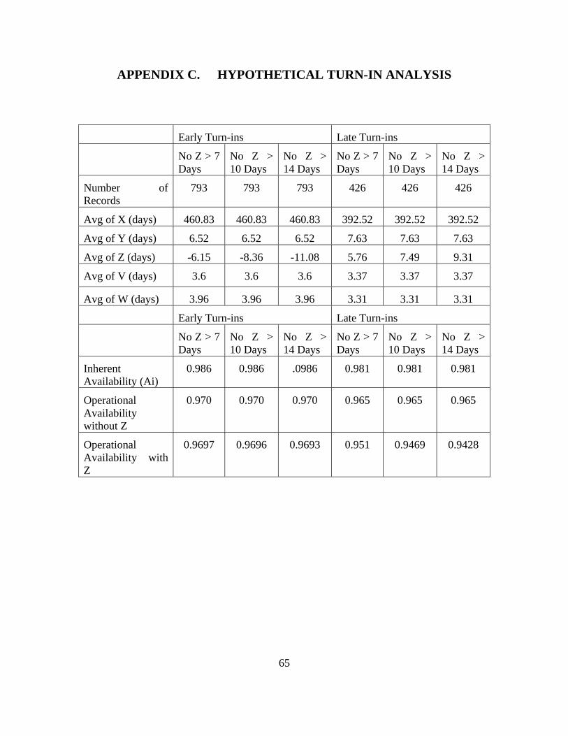
65

APPENDIX C. HYPOTHETICAL TURN-IN ANALYSIS

Early Turn-ins Late Turn-ins

No Z > 7 Days

No Z > 10 Days

No Z > 14 Days

No Z > 7 Days

No Z > 10 Days

No Z > 14 Days

Number of Records

793 793 793 426 426 426

Avg of X (days) 460.83 460.83 460.83 392.52 392.52 392.52

Avg of Y (days) 6.52 6.52 6.52 7.63 7.63 7.63

Avg of Z (days) -6.15 -8.36 -11.08 5.76 7.49 9.31

Avg of V (days) 3.6 3.6 3.6 3.37 3.37 3.37

Avg of W (days) 3.96 3.96 3.96 3.31 3.31 3.31

Early Turn-ins Late Turn-ins

No Z > 7 Days

No Z > 10 Days

No Z > 14 Days

No Z > 7 Days

No Z > 10 Days

No Z > 14 Days

Inherent Availability (Ai)

0.986 0.986 .0986 0.981 0.981 0.981

Operational Availability without Z

0.970 0.970 0.970 0.965 0.965 0.965

Operational Availability with Z

0.9697 0.9696 0.9693 0.951 0.9469 0.9428

66


67

LIST OF REFERENCES

Albright, Jon D. (1997). Reliability enhancement of the navy metrology and calibration program. (Master’s Thesis, Naval Postgraduate School, 1997).

Bonnett, Chris. (2005, August). Change solves navy's quality challenges. Quality 44, no. 8, 36.

Cox, Hill. (2005, January). Get calibration scheduled right. Quality 44, no. 1, 28.

Cox, Hill. (2005, April). Recalibrating intervals. Quality 44, no. 4, 18.

Defense Logistics Agency. (2006). Federal Logistics (FEDLOG) (Compact Disc). Retrieved September 15, 2006.

Department of the Navy. (n.d.). Promulgating metrology automated system for uniform recall and reporting (MEASURE) users manual (OPNAV Manual OP43P6B), Washington, D.C: Chief of Naval Operations.

Department of the Navy. (1986). Technical requirements for technical review of calibration intervals (NAVAIR 17-35TR-06), Patuxent River, M.D.: Commander, Naval Air Systems Command.

Department of the Navy. (1987). Navy calibration activity list (NCA) (NAVAIR 17-35NCA-1), Patuxent River, M.D.: Commander, Naval Air Systems Command.

Department of the Navy. (1990). Department of the navy policy and responsibility for test and measurement, monitoring, diagnostic equipment and systems, and metrology and calibration (METCAL) ( SECNAVINST 3960.6), Washington, D.C.: Secretary of the Navy.

Department of the Navy. (1992). Technical requirements for calibration interval establishment of test and monitoring system (TAMS) (NAVAIR 17-35TR-05), Patuxent River, M.D.: Commander, Naval Air Systems Command.

Department of the Navy, (1998). Manual of navy total force manpower policies and procedures (OPNAVINST 1000.16J), Washington, D.C: Chief of Naval Operations.

Department of the Navy. (2000). Metrology and calibration program operations process manual (NAVAIR 17-35POP-01), Patuxent River, M.D.: Commander, Naval Air Systems Command.

Department of the Navy. (2000). Navy training system plan for the navy metrology and calibration program Navy Training Systems Plan. N88-NTSP-A-50-8701B/A. Retrieved October 26, 2006, from http://www.globalsecurity.org/military/library/policy/navy/ntsp/metcal-A.htm

68

Department of the Navy. (2001). Metrology and calibration quality assurance program (NAVAIRINST 13640.3) Patuxent River, M.D.: Commander, Naval Air Systems Command.

Department of the Navy. (2003). Operational availability of equipments and weapons systems (OPNAVINST 3000.12A), Washington, D.C: Chief of Naval Operations.

Department of the Navy. (2005). Navy test, measurement, and diagnostic equipment (TMDE), automatic test systems (ATS), and metrology and calibration (METCAL) (OPNAVINST 3960.16A), Washington, D.C: Chief of Naval Operations.

Department of the Navy. (2005). Naval aviation maintenance program (NAMP)(COMNAVAIRFORINST 4790.2), San Diego, C.A.: Commander, Naval Air Forces.

Department of the Navy. Naval Aviation Systems Command (NAVAIR), NAVAIR AirSpeed Program. Retrieved October 26, 2006, from http://www.navair.navy.mil/navairairspeed.

Department of the Navy, Naval Surface Warfare Center (NSWC), Corona Division. Measurement and science department core functions. Retrieved October 26, 2006, from http://www.corona.navy.mil.

Helicopter Maritime Strike Squadron Forty-One (HSM-41). Mission Statement. Retrieved September 2006, from http://www.hsl41.navy.mil

Helicopter Anti Submarine Squadron Light Forty-Three (HSL-43). Mission Statement. Retrieved September 2006, from http:/www.hsl43.navy.mil

Landreth, C. J., Wilhelm II, R. H., & Corporon, L. L. (2005). Performance based logistics (PBL) for the FA-18. (MBA Professional Report, Naval Postgraduate School, 2005).

Mitchell, M. A., & Pasch, J. E. (1996). Calibration laboratories as a regional repair center: consolidate or collocate. (MBA Professional Report, Naval Postgraduate School, 1996).

Snowden, T. M., & Sullivan, D. R. (2005). Filling H-60 helicopter readiness shortfalls by streamlining and revising depot level maintenance procedures. (MBA Professional Report, Naval Postgraduate School, 2005).

Wickberg, E., & Twining, T. (2002, July). Improvements to pressure sensing instruments enable new practices. Control Engineering Europe. Retrieved July 24, 2006 from http://www.manufacturing.net/ctl/

Wickberg, E., Twining, T., & Kent, D. (2002, October). Instrument technology improvements spur predictive maintenance programmes. Control Engineering Europe. Retrieved July 24, 2006 from http://www.manufacturing.net/ctl/

69

United States Marine Corps. Logistics Modernization (LOGMod). Marine Air-Ground Task Force Distribution. Retrieved November 07, 2006, from https://logmod.hqmc.usmc.mil/Initiatives_MAGTF_Distro.htm.

70


71

INITIAL DISTRIBUTION LIST

1. Defense Technical Information Center Ft. Belvoir, Virginia

2. Dudley Knox Library Naval Postgraduate School Monterey, California

3. Marine Corps Representative Naval Post Graduate School Monterey, California

4. Director Training and Education, MCCDC, Code C46 Quantico, Virginia

5. Director, Marine Corps Research Center, MCCDC, Code C40RC Quantico, Virginia

6. Marine Corps Tactical Systems Support Activity (Attn: Operations Officer) Camp Pendleton, California

7. COMHELMARSTRIKEWINGPAC, Attn:, METCAL Representative San Diego, California

8. On-Site Operations Manager MOCC San Diego, California

9. NAVAIR METCAL DPM NAVAIRSYSCOM Patuxent River, Maryland

10. Professor Keebom Kang Naval Postgraduate School Monterey, California

11. Professor Uday Apte Naval Postgraduate School Monterey, California

12. Capt Robert Stonaker Naval Postgraduate School Monterey, California

72

13. Capt Kelly Johnson Naval Postgraduate School Monterey, California

14. Capt Kenneth Bevel Naval Postgraduate School Monterey, California

15. GySgt Amy Pearson

MCLO NSWC Corona Corona, California

Documents

NAVAL POSTGRADUATE · PDF fileA. NAVAL AVIATION METROLOGY AND CALIBRATION ... Metrology and Calibration Definitions ... Naval Postgraduate School