National Center for Atmospheric Research

P. O. Box 3000 Boulder, Colorado

80307-3000 www.ucar.edu

NCAR Technical Notes NCAR/TN-542+STR

Population Projections for US States under the Shared Socioeconomic Pathways Based on Global Gridded Population Projections

Leiwen Jiang Hamidreza Zoraghein Brian C. O’Neill

NCAR IS SPONSORED BY THE NSF

NCAR TECHNICAL NOTES http://library.ucar.edu/research/publish-technote

The Technical Notes series provides an outlet for a variety of NCAR Manuscripts that contribute in specialized ways to the body of scientific knowledge but that are not yet at a point of a formal journal, monograph or book publication. Reports in this series are issued by the NCAR scientific divisions, serviced by OpenSky and operated through the NCAR Library. Designation symbols for the series include:

EDD – Engineering, Design, or Development Reports Equipment descriptions, test results, instrumentation, and operating and maintenance manuals.

IA – Instructional Aids Instruction manuals, bibliographies, film supplements, and other research or instructional aids.

PPR – Program Progress Reports Field program reports, interim and working reports, survey reports, and plans for experiments.

PROC – Proceedings Documentation or symposia, colloquia, conferences, workshops, and lectures. (Distribution maybe limited to

attendees).

STR – Scientific and Technical Reports Data compilations, theoretical and numerical investigations, and experimental results.

The National Center for Atmospheric Research (NCAR) is operated by the nonprofit University Corporation for Atmospheric Research (UCAR) under the sponsorship of the National Science Foundation. Any opinions, findings, conclusions, or recommendations expressed in this publication are those of the author(s) and do not necessarily reflect the views of the National Science Foundation.

National Center for Atmospheric Research P. O. Box 3000

Boulder, Colorado 80307-3000

i

NCAR/TN-542+STR NCAR Technical Note

______________________________________________

January 2018

Population Projections for US States under the Shared Socioeconomic Pathways Based on Global Gridded

Population Projections

Leiwen Jiang Climate & Global Dynamics Lab, Integrated Assessment Modeling Group National Center for Atmospheric Research, Boulder, Colorado

Hamidreza Zoraghein Climate & Global Dynamics Lab, Integrated Assessment Modeling Group National Center for Atmospheric Research, Boulder, Colorado

Brian C. O’Neill Climate & Global Dynamics Lab, Integrated Assessment Modeling Group National Center for Atmospheric Research, Boulder, Colorado

Climate & Global Dynamics Laboratory

______________________________________________________ NATIONAL CENTER FOR ATMOSPHERIC RESEARCH

P. O. Box 3000 BOULDER, COLORADO 80307-3000

ISSN Print Edition 2153-2397 ISSN Electronic Edition 2153-2400

ii

Contents

List of Figures ..................................................................................... iv

Acknowledgments ................................................................................. v

1 Introduction ...................................................................................... 1

2 Data and Methods .............................................................................. 2

2.1 Data ..................................................................................... 2

2.2 Methods ................................................................................ 3

3 Evaluation of methods and base year spatial distribution ....................... 5

4 Evaluation of projections................................................................... 12

5 Discussions and Conclusions ............................................................. 21

References ........................................................................................ 23

Appendix .......................................................................................... 24

iii

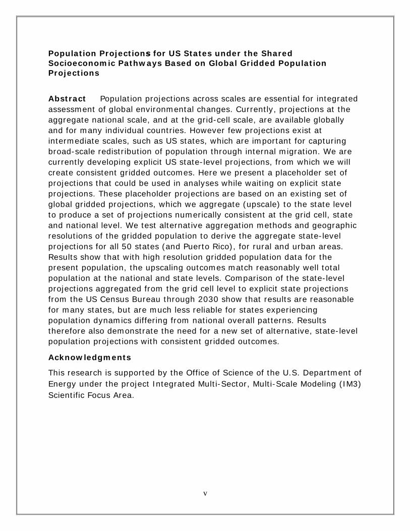
List of Figures Figure 1: Comparison of the US population numbers from different sources in 2000

Figure 2: Difference of US state population aggregated from the gridded data to the Census records, 2000

Figure 3: The spatial gridded population of Hawaii in 2000 at 1/8 degree resolution

Figure 4: The spatial gridded population within the buffered US administrative boundary

Figure 5: US population derived from the gridded population with/out applying buffered boundary

Figure 6: Projections of the US total, rural and urban population under SSP scenarios

Figure 7: US state population projections from the upscaling and the US Census Bureau

Figure 8: Percentage of changes in the share of US state population to the national total

Appendix 1: Aggregated SSPs state total population projections (in green) compared to the Census records (in black) and the Census Bureau projections (in red)

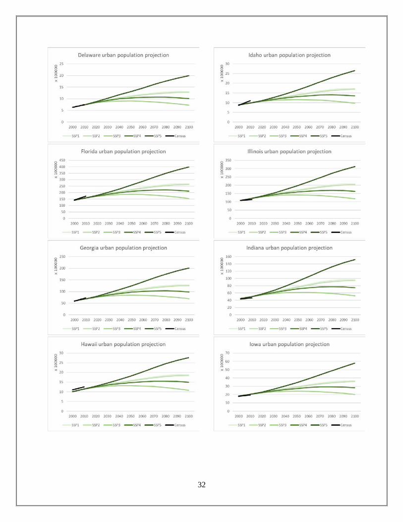
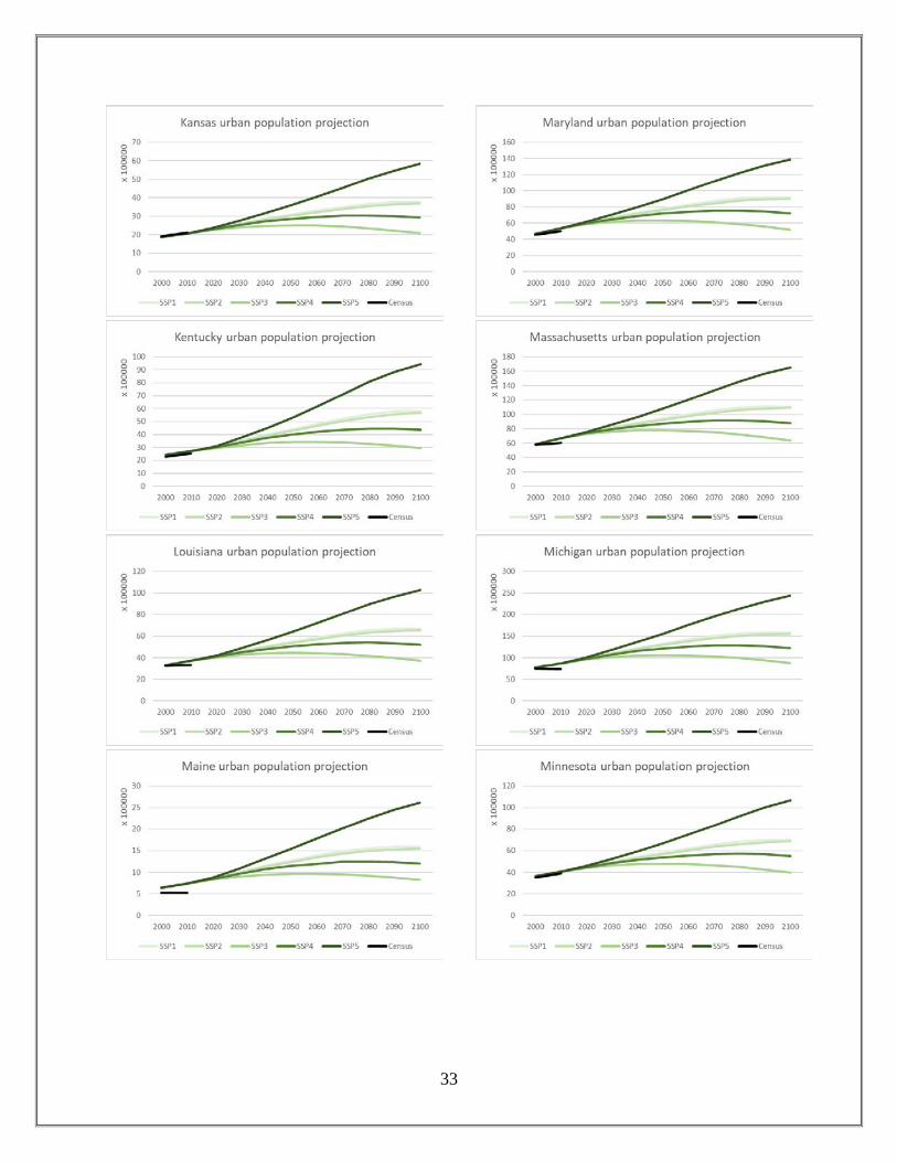
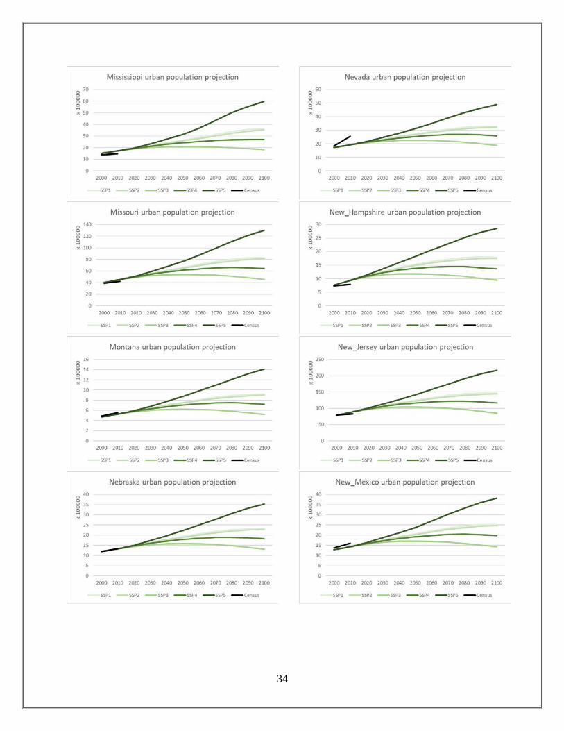
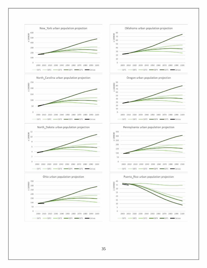
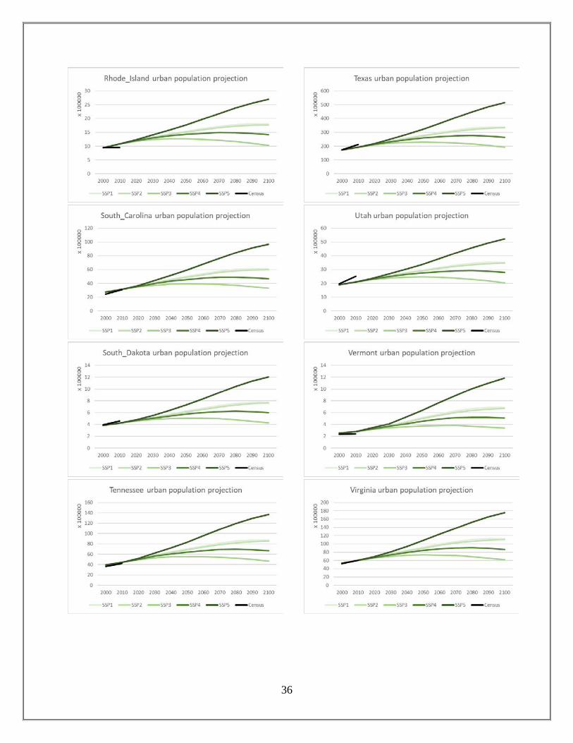
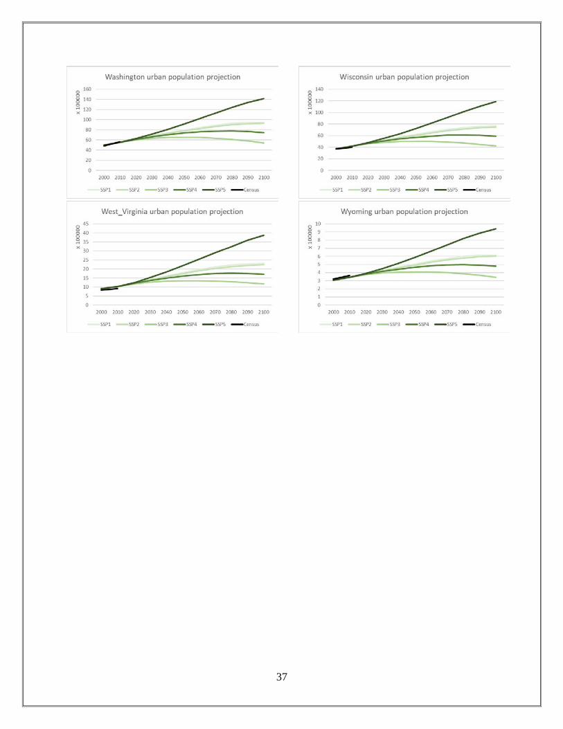
Appendix 2: Aggregated SSPs state urban population projections (in green) compared to the Census records (in black)

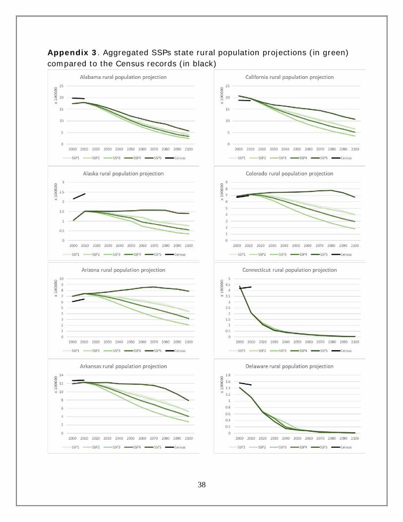
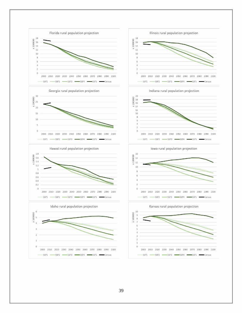
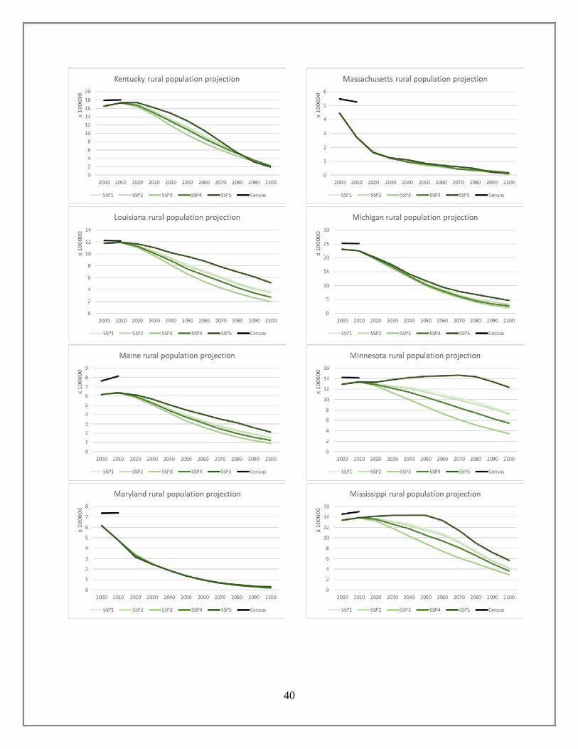
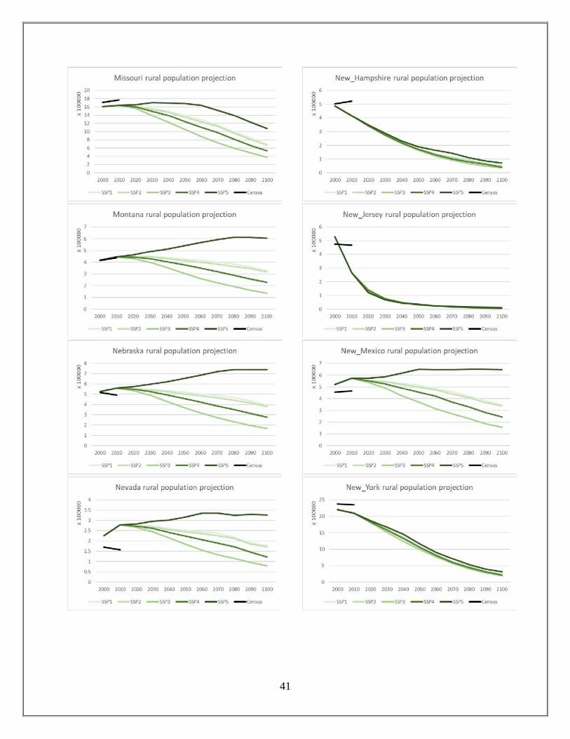
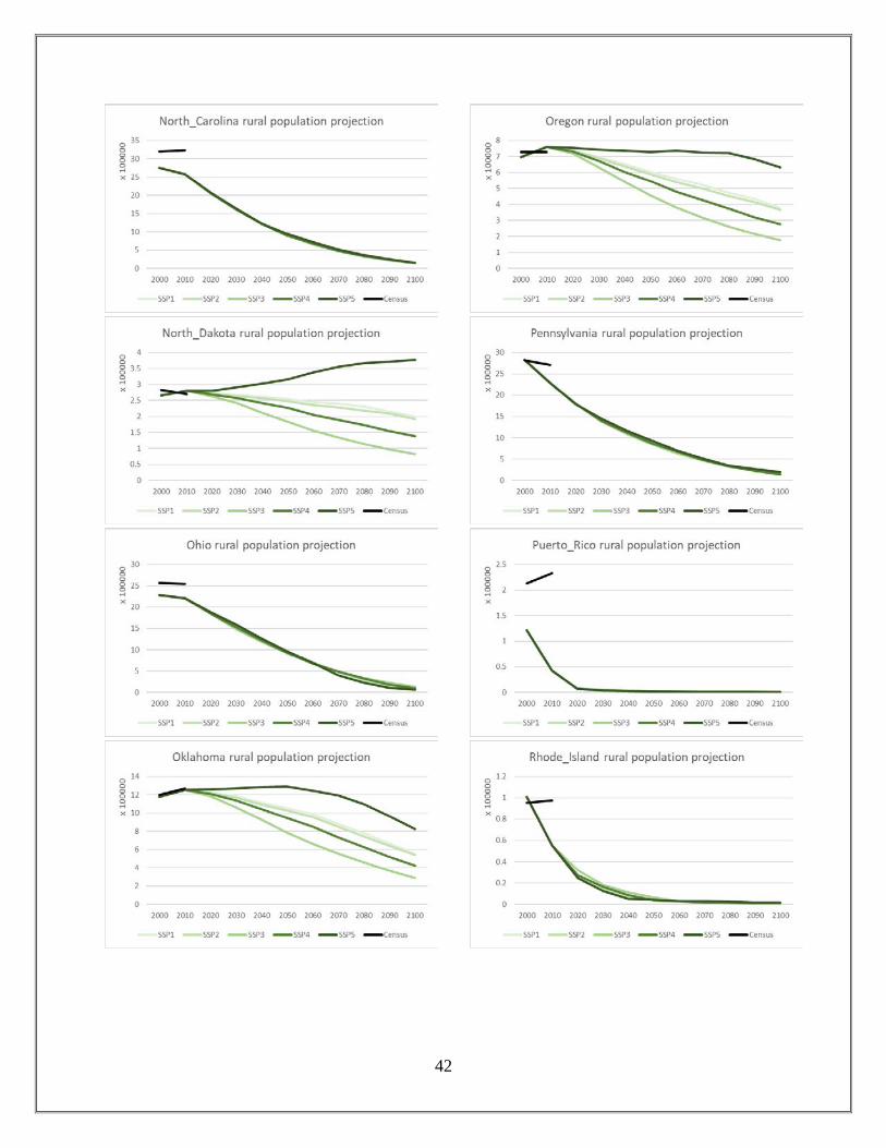
Appendix 3: Aggregated SSPs state rural population projections (in green) compared to the Census records (in black)

iv

Population Projections for US States under the Shared Socioeconomic Pathways Based on Global Gridded Population Projections

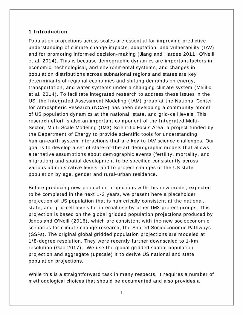
Abstract Population projections across scales are essential for integrated assessment of global environmental changes. Currently, projections at the aggregate national scale, and at the grid-cell scale, are available globally and for many individual countries. However few projections exist at intermediate scales, such as US states, which are important for capturing broad-scale redistribution of population through internal migration. We are currently developing explicit US state-level projections, from which we will create consistent gridded outcomes. Here we present a placeholder set of projections that could be used in analyses while waiting on explicit state projections. These placeholder projections are based on an existing set of global gridded projections, which we aggregate (upscale) to the state level to produce a set of projections numerically consistent at the grid cell, state and national level. We test alternative aggregation methods and geographic resolutions of the gridded population to derive the aggregate state-level projections for all 50 states (and Puerto Rico), for rural and urban areas. Results show that with high resolution gridded population data for the present population, the upscaling outcomes match reasonably well total population at the national and state levels. Comparison of the state-level projections aggregated from the grid cell level to explicit state projections from the US Census Bureau through 2030 show that results are reasonable for many states, but are much less reliable for states experiencing population dynamics differing from national overall patterns. Results therefore also demonstrate the need for a new set of alternative, state-level population projections with consistent gridded outcomes.

Acknowledgments

This research is supported by the Office of Science of the U.S. Department of Energy under the project Integrated Multi-Sector, Multi-Scale Modeling (IM3) Scientific Focus Area.

v

1 Introduction

Population projections across scales are essential for improving predictive understanding of climate change impacts, adaptation, and vulnerability (IAV) and for promoting informed decision-making (Jiang and Hardee 2011; O’Neill et al. 2014). This is because demographic dynamics are important factors in economic, technological, and environmental systems, and changes in population distributions across subnational regions and states are key determinants of regional economies and shifting demands on energy, transportation, and water systems under a changing climate system (Melillo et al. 2014). To facilitate integrated research to address these issues in the US, the Integrated Assessment Modeling (IAM) group at the National Center for Atmospheric Research (NCAR) has been developing a community model of US population dynamics at the national, state, and grid-cell levels. This research effort is also an important component of the Integrated Multi-Sector, Multi-Scale Modeling (IM3) Scientific Focus Area, a project funded by the Department of Energy to provide scientific tools for understanding human-earth system interactions that are key to IAV science challenges. Our goal is to develop a set of state-of-the-art demographic models that allows alternative assumptions about demographic events (fertility, mortality, and migration) and spatial development to be specified consistently across various administrative levels, and to project changes of the US state population by age, gender and rural-urban residence.

Before producing new population projections with this new model, expected to be completed in the next 1-2 years, we present here a placeholder projection of US population that is numerically consistent at the national, state, and grid-cell levels for internal use by other IM3 project groups. This projection is based on the global gridded population projections produced by Jones and O’Neill (2016), which are consistent with the new socioeconomic scenarios for climate change research, the Shared Socioeconomic Pathways (SSPs). The original global gridded population projections are modeled at 1/8-degree resolution. They were recently further downscaled to 1-km resolution (Gao 2017). We use the global gridded spatial population projection and aggregate (upscale) it to derive US national and state population projections.

While this is a straightforward task in many respects, it requires a number of methodological choices that should be documented and also provides a

1

useful illustration of the shortcomings of current spatial projections for large countries, which could be improved through sub-national projections such as those planned within the IM3 project for the US. This Technical Note therefore documents the data and methods used for deriving the US national and state projections for urban and rural populations from the global gridded population projections under the SSP scenarios. The upscaled national and state populations from the spatial gridded data at both 1/8 degree and 1-km resolutions are compared to the US census data in the base year 2000, and the projected state total populations are compared to census data for the period 2000-2010 and to short-term state population projections (up to 2030) produced by the US Census Bureau (2005). The analysis of differences between the upscaled state population projections and the census data and projections suggests shortcomings of the upscaling approach and provides caveats for the use of the current projection results. We finally discuss needs for deriving better projection outcomes through conducting explicit state population projections.

2 Data and Methods

2.1. Data

We use the global gridded spatial population projections under the SSP scenarios to derive future rural and urban population for the US as a whole and its 50 states (as well as Puerto Rico). The global gridded population projections are produced using a spatial population downscaling model (Jones and O’Neill 2016), based on the combined outputs of national population projections (KC and Lutz 2015) and urbanization projections (Jiang and O’Neill 2015) for all countries under the SSP scenarios.

In the global gridded population projections, Jones and O’Neill (2016) use an extended population gravity model to allocate changes in the national total rural and urban population to grid cells at 1/8 degree (or approximately 12-km) resolution according to an index of their potential attractiveness. The population potential surfaces for both rural and urban population are modeled based on the spatial population distribution in a given year and gravity model parameters estimated from historical population changes and geographic conditions.

Jones and O’Neill (2016) produce their own spatial urban and rural population distributions for the base year (2000) and for 1990 based on data from the Gridded Population of the World (version 3, CIESIN et al. 2005). The GPW population data are at the resolution of 2.5 arc-minutes and are

2

generally based on national Census data where available. However, the data do not distinguish urban from rural populations. To add this feature, Jones and O’Neill draw on urban extent grids that distinguish urban and rural land areas from the Global Rural-Urban Mapping Project (GRUMP, Balk 2006). They first assign all GPW population in grid cells within GRUMP urban land areas to be urban. Next, they add or subtract grid cells to or from the urban category until the aggregate GPW population over those grid cells matches an exogenously-defined urban total.1 They assign population in the remaining grid cells to be rural. Finally, they add up the rural and urban populations within each 1/8 degree grid cell used in the projection. The resulting 1/8 degree urban and rural population map for the year 2000 serves as the starting point for global spatial projections.

Taking the global gridded spatial population projections at 1/8 degree resolution as a starting point, Gao (2017) recently produced a set of new results with higher geographic resolution in which the population of each 1/8 degree grid at each time step in the projection is further downscaled to 1-km resolution. This downscaling was carried out by assuming that the proportion of population in each 1/8 grid cell located in each 1-km sub-grid cell remained fixed at the pattern observed in the GRUMP data in the year 2000. Here we use both sets of gridded population projections (1/8 degree and 1-km resolutions) to derive aggregate urban and rural population projections for the US as a whole and its 50 states.

2.2 Method

We use the 1/8-degree and 1-km gridded population projections, overlay them with US state administrative boundaries, and add populations within grid cells up to the state and national levels. We first upscale rural and urban populations separately, and add them together to derive the state total population.

The key methodological choice to make is how to deal with population in grid cells that straddle borders – between states, between countries, and on coast lines, with some grid cells straddling more than one type of border. We test two spatial aggregation methods – the centroid method and proportional method – for the upscaling process. In the former, all the population of a grid cell is allocated to the single state within which the geographic centroid of the grid cell falls. In the latter, the population of a grid cell is proportionately allocated to the intersecting state(s) (and countries and

1 The exogenously defined total rural and urban populations for each country are taken from Jiang and O’Neill (2015), which is based on the data from the UN World Population Prospects 2012 Revision (United National 2013) and UN World Urbanization Prospects 2011 Revision (United Nations 2012).

3

water bodies, if relevant) according to the area of that grid cell that overlaps with the state or other region. These methods can be thought of as making two contrasting assumptions about the (unknown) sub-grid cell distribution of population: the proportional method assumes population is distributed uniformly over space, while the centroid method assumes all population is located at the centroid.

The relative accuracy of the two methods is difficult to predict ahead of time without having some expectations of the true sub-grid cell population distribution. The centroid method will be more accurate in situations in which population distribution happens to be more concentrated and skewed toward the state in which the centroid falls. But it will be less accurate when population distribution is skewed outside of that state, or when the distribution is relatively even. A special case of this general rule occurs at coast lines, where the true population distribution is completely skewed toward the land area. If the centroid falls on land, it will accurately assign all population to the state; if it does not, it will make a larger error than the proportional method would in assigning population to the water body.

In either method, it can be expected that the higher resolution (1 km) projection will more accurately reflect state and national totals, because relative to the coarser projection it benefits from information on the population distribution within the 1/8 degree grid cell.

Note that there are two reasons that either method, with either resolution, could produce national population totals that do not match the total US population that was assumed in the global spatial projections from Jones and O’Neill. The global projection results are in the form of urban and rural population totals for each grid cell, globally. Grid cells that fall on national borders do not include information on the proportion of population within the grid cell that belongs to each country. The upscaling method makes its own estimate of what those proportions are (either 0/1, in the centroid method, or a proportion based on geographic area), and these will not generally be completely accurate. In addition, the upscaling method as applied here can inaccurately assign population in grid cells on coast lines to water bodies, rather than to the country to which they belong. The method could be modified to assign all population to a state if a cell is shared with a water body. However, this would substantially increase computing time, especially for the 1 km projections, and so is not pursued here.

4

3 Evaluation of methods and base year spatial distribution

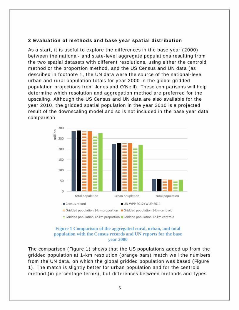
As a start, it is useful to explore the differences in the base year (2000) between the national- and state-level aggregate populations resulting from the two spatial datasets with different resolutions, using either the centroid method or the proportion method, and the US Census and UN data (as described in footnote 1, the UN data were the source of the national-level urban and rural population totals for year 2000 in the global gridded population projections from Jones and O’Neill). These comparisons will help determine which resolution and aggregation method are preferred for the upscaling. Although the US Census and UN data are also available for the year 2010, the gridded spatial population in the year 2010 is a projected result of the downscaling model and so is not included in the base year data comparison.

Figure 1 Comparison of the aggregated rural, urban, and total population with the Census records and UN reports for the base

year 2000

The comparison (Figure 1) shows that the US populations added up from the gridded population at 1-km resolution (orange bars) match well the numbers from the UN data, on which the global gridded population was based (Figure 1). The match is slightly better for urban population and for the centroid method (in percentage terms), but differences between methods and types

0

50

100

150

200

250

300

total population urban pouplation rural population

mill

ion

Census record UN WPP 2012+WUP 2011

Gridded population 1-km proportion Gridded population 1-km centroid

Gridded population 12-km proportion Gridded population 12-km centroid

5

of population are not large. Note that, as discussed in section 2.2., inaccuracies in upscaling to national totals can occur due to misallocation of population in grid cells falling on coastlines or national borders.

The match to the UN data is not as good for the populations aggregated from the 1/8 degree spatial distribution (green bars). When comparing results based on either the 1/8 degree or 1-km data, the 1 km results are more accurate in urban areas, while results are similar in rural areas when using either aggregation method, i.e., both estimates are slightly lower than the UN report.

Thus at the national level, base year aggregate populations can be successfully produced from the spatial data. Totals are reproduced significantly better by the 1 km spatial distribution, particularly for urban population. Also, the centroid method slightly outperforms the proportional method, and significantly so for urban population in the 1/8 degree dataset.

To examine the upscaled results at the state level, we compare aggregate state populations to the US 2000 Census records, since the UN World Population Prospects and Urbanization Prospects datasets do not have subnational statistics. It should be noted that the US 2000 Census data does not exactly equal the UN report in terms of total population; it estimates a slightly smaller total population size for the US (Figure 1). Compared to the US census records, the state-level total population values aggregated from the gridded population at 1-km resolution are very similar for most states; the absolute differences are less than 1% of the actual state totals (Figure 2a). There are only a few states with differences larger than 1%, and they are mostly island or coastal states (e.g., Florida, Alaska, Hawaii, Rhode Island, Maine, and Delaware). Using the centroid aggregation method reaches similar or even better results for some states than using the proportional method.

6

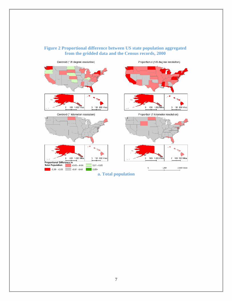
Figure 2 Proportional difference between US state population aggregated from the gridded data and the Census records, 2000

a. Total population

7

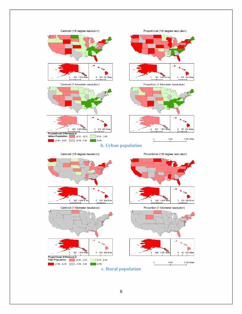
b. Urban population

c. Rural population

8

In contrast, state total populations added up from the coarse 1/8th degree resolution dataset deviate significantly more from the census records. Using the proportional method, the populations aggregated from the 1/8th resolution dataset are systematically lower than the census records in a majority of states, while the aggregated populations using the centroid method indicate both under- and over-estimates across different states.

Errors in state totals of urban and rural population (Figure 2b and 2c) are significantly larger than for the two populations combined (Figure 2a). This is true for results derived from both spatial data resolutions, although results from the 1-km resolution dataset are somewhat better than those from the 1/8 degree dataset. The errors are similar when using either the centroid or the proportion method. The larger errors in urban and rural totals, and relative lack of dependence on the spatial data resolution and aggregation method, suggest that the reason for this inaccuracy is in the methodology used by Jones and O’Neill (2016) in producing the spatial distribution of urban and rural population. As discussed in Section 2, the approach used the GRUMP urban extent data to assign population to the urban category. This likely resulted in some strong differences with the census-based definition of where urban population is located in the base year.

Thus as was the case for the national level, state-level total population can be successfully derived in the base year by aggregating the spatial population distribution, with significantly better results when using the 1 km distribution. State-level total rural and urban populations are significantly less well reproduced, most likely due to errors in the spatial distributions rather than in the aggregation methods.

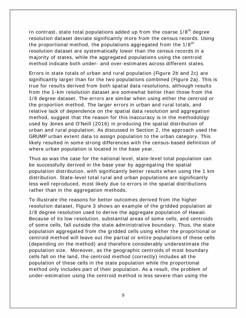
To illustrate the reasons for better outcomes derived from the higher resolution dataset, Figure 3 shows an example of the gridded population at 1/8 degree resolution used to derive the aggregate population of Hawaii. Because of its low resolution, substantial areas of some cells, and centroids of some cells, fall outside the state administrative boundary. Thus, the state population aggregated from the gridded cells using either the proportional or centroid method will leave out the partial or entire populations of these cells (depending on the method) and therefore considerably underestimate the population size. Moreover, as the geographic centroids of most boundary cells fall on the land, the centroid method (correctly) includes all the population of these cells in the state population while the proportional method only includes part of their population. As a result, the problem of under-estimation using the centroid method is less severe than using the

9

proportional method, which allocates part of the population of the boundary cells to the ocean.

Compared to the original 1/8 degree resolution dataset, the gridded population at 1-km resolution substantially improves the spatial distribution of population and greatly diminishes the allocation of population to the ocean or other water bodies. When downscaling population from 1/8 degree to 1 km, zero weight is assigned to 1 km grid cells not located over land, greatly reducing the population that could be incorrectly assigned to the ocean rather than to the land during the upscaling process. This in turn results in rather similar aggregated state-level populations using either the proportion or the centroid method.

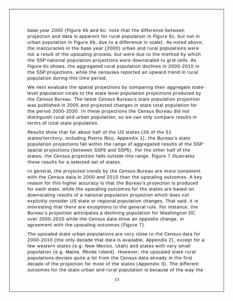
To avoid missing population in coastal areas, one could consider placing a buffer around the coastlines. For example, using a buffered boundary, the population cells of the small islands of Hawaii are successfully contained and accounted for while aggregating them to the state boundary (Figure 3b). However, the buffered boundary could also contribute to over-estimated population values near national borders by wrongly including population from neighboring countries, e.g., some portion of the Canadian population adjacent to the boundaries of northeast Vermont and northwest Washington are erroneously assigned to these states (Figure 4). Figure 5 shows that after applying the buffered boundary, the national populations aggregated from both the 1/8 degree resolution and 1-km resolution datasets become quite similar but are all larger than the census records. While one might reduce the error by adopting more complicated methods and placing buffers only around coastlines, the buffered boundary is problematic in some cases because it creates artificial overlapping areas in coastal states, making them no longer mutually exclusive. This jeopardizes achieving consistent outcomes in those states.

Based on our analysis of the base year population, we adopt the global gridded population projections at 1-km resolution and use the centroid aggregation method to derive the total, rural and urban population projections for the US as a whole and for its individual states (also including Puerto Rico).

10

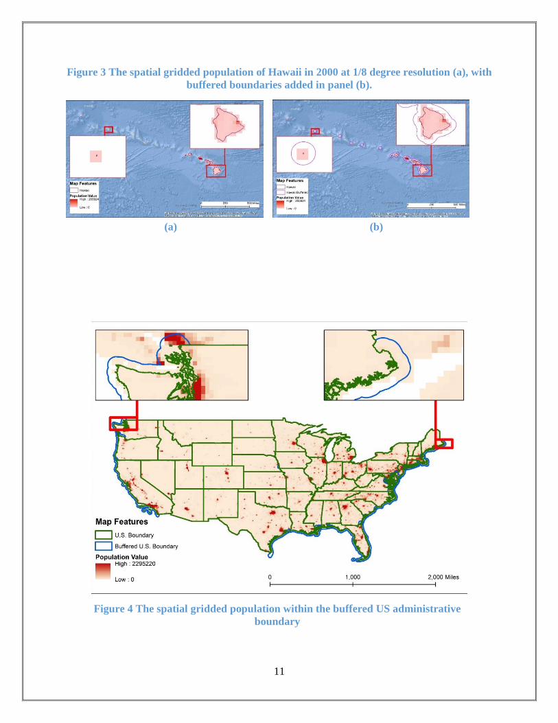
Figure 3 The spatial gridded population of Hawaii in 2000 at 1/8 degree resolution (a), with buffered boundaries added in panel (b).

(a) (b)

Figure 4 The spatial gridded population within the buffered US administrative boundary

11

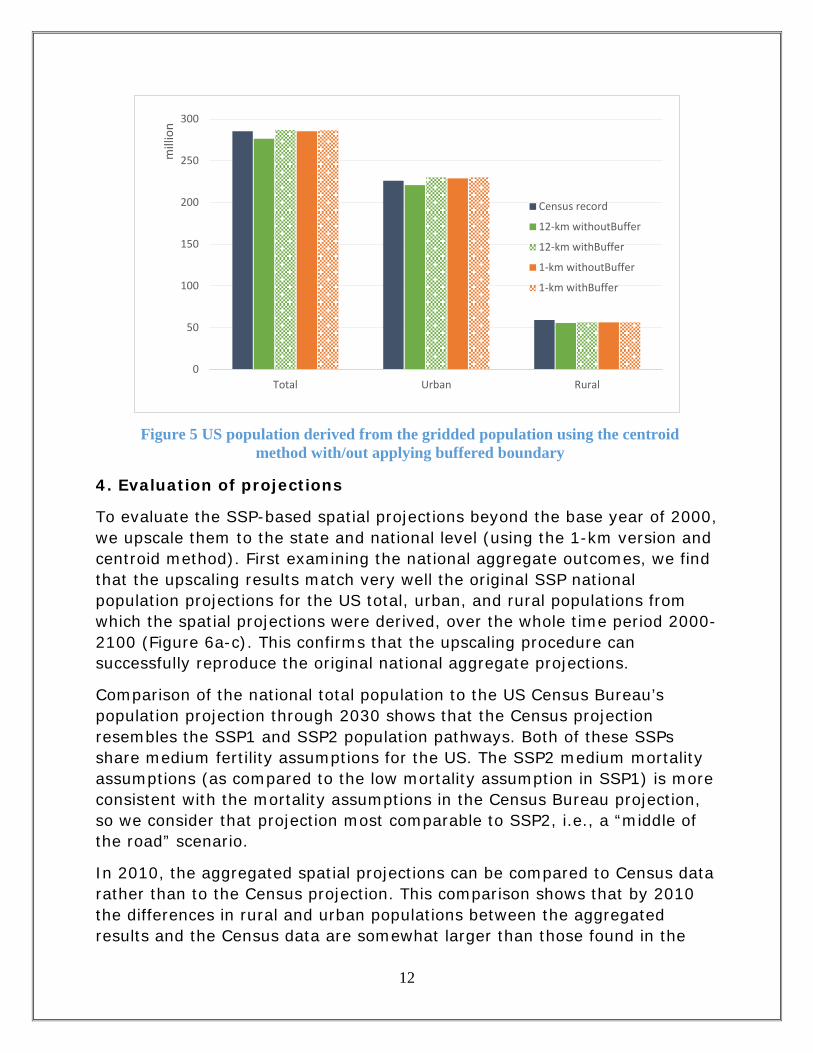
Figure 5 US population derived from the gridded population using the centroid method with/out applying buffered boundary

4. Evaluation of projections

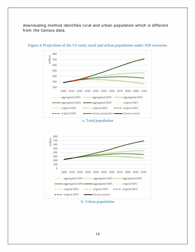
To evaluate the SSP-based spatial projections beyond the base year of 2000, we upscale them to the state and national level (using the 1-km version and centroid method). First examining the national aggregate outcomes, we find that the upscaling results match very well the original SSP national population projections for the US total, urban, and rural populations from which the spatial projections were derived, over the whole time period 2000-2100 (Figure 6a-c). This confirms that the upscaling procedure can successfully reproduce the original national aggregate projections.

Comparison of the national total population to the US Census Bureau’s population projection through 2030 shows that the Census projection resembles the SSP1 and SSP2 population pathways. Both of these SSPs share medium fertility assumptions for the US. The SSP2 medium mortality assumptions (as compared to the low mortality assumption in SSP1) is more consistent with the mortality assumptions in the Census Bureau projection, so we consider that projection most comparable to SSP2, i.e., a “middle of the road” scenario.

In 2010, the aggregated spatial projections can be compared to Census data rather than to the Census projection. This comparison shows that by 2010 the differences in rural and urban populations between the aggregated results and the Census data are somewhat larger than those found in the

0

50

100

150

200

250

300

Total Urban Rural

mill

ion

Census record

12-km withoutBuffer

12-km withBuffer

1-km withoutBuffer

1-km withBuffer

12

base year 2000 (Figure 6b and 6c; note that the difference between projection and data is apparent for rural population in Figure 6c, but not in urban population in Figure 6b, due to a difference in scale). As noted above, the inaccuracies in the base year (2000) urban and rural populations were not a result of the upscaling process, but were due to the method by which the SSP national population projections were downscaled to grid cells. As Figure 6c shows, the aggregated rural population declines in 2000-2010 in the SSP projections, while the censuses reported an upward trend in rural population during this time period.

We next evaluate the spatial projections by comparing their aggregate state-level population totals to the state level population projections produced by the Census Bureau. The latest Census Bureau’s state population projection was published in 2005 and projected changes in state total population for the period 2000-2030. In these projections the Census Bureau did not distinguish rural and urban population, so we can only compare results in terms of total state population.

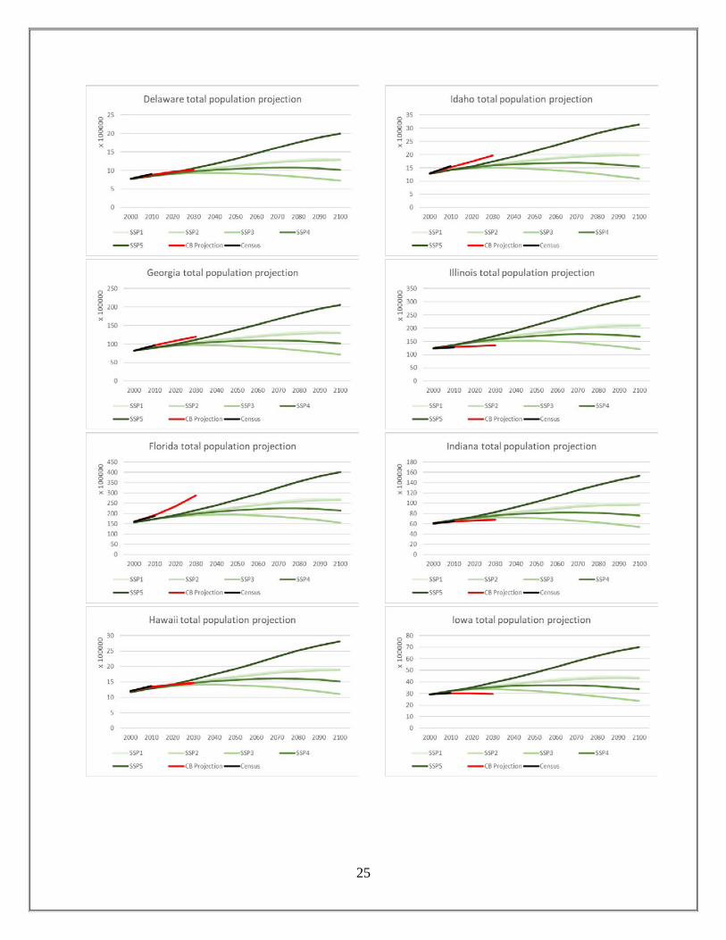
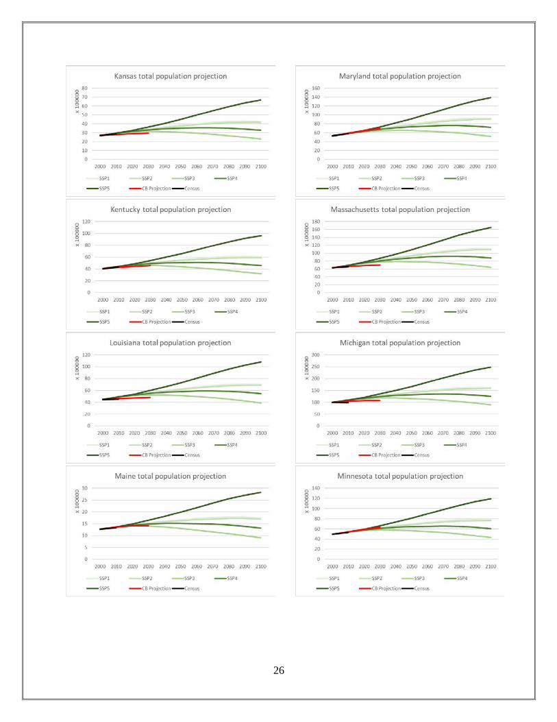
Results show that for about half of the US states (26 of the 51 states/territory, including Puerto Rico, Appendix 1), the Bureau’s state population projections fall within the range of aggregated results of the SSP spatial projections (between SSP3 and SSP5). For the other half of the states, the Census projection falls outside this range. Figure 7 illustrates these results for a selected set of states.

In general, the projected trends by the Census Bureau are more consistent with the Census data in 2000 and 2010 than the upscaling outcomes. A key reason for this higher accuracy is that the Bureau’s projection is produced for each state, while the upscaling outcomes for the states are based on downscaling results of a national population projection which does not explicitly consider US state or regional population changes. That said, it is interesting that there are exceptions to the general rule. For instance, the Bureau’s projection anticipates a declining population for Washington DC over 2000-2010 while the Census data show an opposite change, in agreement with the upscaling outcomes (Figure 7).

The upscaled state urban populations are very close to the Census data for 2000-2010 (the only decade that data is available, Appendix 2), except for a few western states (e.g. New Mexico, Utah) and states with very small population (e.g. Maine, Rhode Island). However, the upscaled state rural populations deviate quite a lot from the Census data already in the first decade of the projection for most of the states (Appendix 3). The different outcomes for the state urban and rural population is because of the way the

13

downscaling method identifies rural and urban population which is different from the Census data.

Figure 6 Projections of the US total, rural and urban population under SSP scenarios

a. Total population

b. Urban population

200

300

400

500

600

700

800

2000 2010 2020 2030 2040 2050 2060 2070 2080 2090 2100

mill

ion

aggregated SSP1 aggregated SSP2 aggregated SSP3

aggregated SSP4 aggregated SSP5 original SSP1

original SSP2 original SSP3 original SSP4

original SSP5 Census projection Census record

0100200300400500600700800

2000 2010 2020 2030 2040 2050 2060 2070 2080 2090 2100

mill

ion

aggregated SSP1 aggregated SSP2 aggregated SSP3

aggregated SSP4 aggregated SSP5 original SSP1

original SSP2 original SSP3 original SSP4

original SSP5 Census record

14

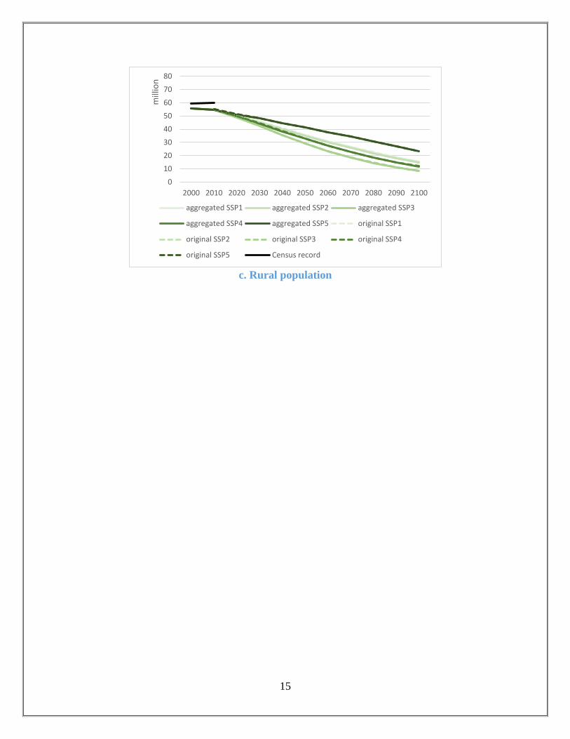
c. Rural population

01020304050607080

2000 2010 2020 2030 2040 2050 2060 2070 2080 2090 2100

mill

ion

aggregated SSP1 aggregated SSP2 aggregated SSP3

aggregated SSP4 aggregated SSP5 original SSP1

original SSP2 original SSP3 original SSP4

original SSP5 Census record

15

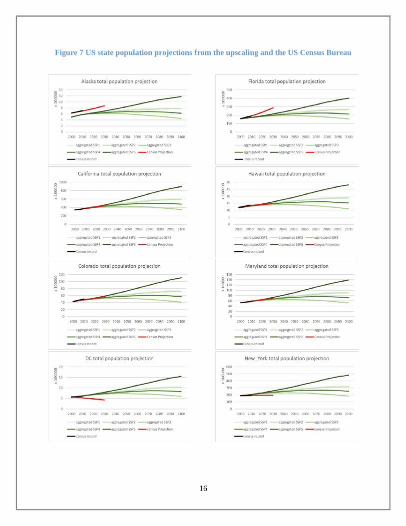
Figure 7 US state population projections from the upscaling and the US Census Bureau

16

To evaluate the effect of the spatial population projection on the broad distribution of population within the US, we compare changes in the percentage of US population residing in each state in the aggregated SSP spatial projections versus the Census Bureau state projections over the period 2000-2030. Results show that the percentages of US population residing in each state change very little change (< 0.1%, where 0.1% is the difference in percentages in the two years, measured in percentage points) by 2030 across the SSPs, except in California and Texas under all SSPs, and New York and Florida under SSP3 (Figure 8a). This indicates that population growth in most states generally follows the national growth rate. This is not unexpected, because the downscaling of national total population for each SSP does not explicitly consider variations across states. In contrast, the state population projections from the Census Bureau anticipate substantial changes in the percentage of population living in many states, most notably a decrease in many northcentral, northeastern, and southcentral states of up to 1% (New York), and an increase in southern and western states of up to 1.7% (Florida). This occurs because the Census Bureau’s projection explicitly considers the population dynamics of individual states, especially changes caused by internal migration flows.

While the percentages of population living in specific states based on the upscaling results do not change much in the short-term, there are somewhat larger population shifts across states in the long-run – by 2100 (Figure 8b-d). The state percentage of total population increases mainly in the Western states (California, Arizona, and Texas), and also Florida in the Southeast, and New Yok in the Northeast; the share decreases mainly in the Central North and Southeast (Figure 8b). The regional population changes across states are most distinct under SSP3 (low population growth and slow urbanization scenario for the US) and the least substantial under SSP5 (high population growth and fast urbanization scenario for the US).

Compared to the changes of total population distribution, changes in rural and urban population distribution across states are very different. State urban population shares of the national urban population grow in most of the states in the east, but decline in the states with big metropolitan areas (California, New York, Illinois, and Florida); the changes are moderate under SSP3, but most significant under SSP5 (Figure 8c). In contrast, rural population shares increase in almost all the states in the west, but decrease in the majority of the states in the east. Similar to urban areas, the changes are the most distinct under SSP5 and less significant under SSP3 (Figure

17

8d). In general, the changes in the share of urban population are quite small (up to -1,5%, with changes in most of the states within 0.1%), because most states are already highly urbanized (above 80% urban) and the room for changes to the large base urban population is limited. In contrast, the changes in state percentages of the total rural population range from -4.3% to +3.2%.

These results reflecting shifts in the distribution of the population in the spatial projections are a consequence of the gravity model used to downscale the projected aggregate population to grid cells. Depending on parameter values, the model preferentially allocates population to areas with existing concentrations of population, which leads to a shift in the spatial distribution of the total population away from the Midwest and towards the West and South. It is also the reason for the differences in the allocation of urban and rural populations, i.e. it reflects differences in the initial distribution of the urban and rural populations in the base year – more urban population in the east and more rural population in the west.

18

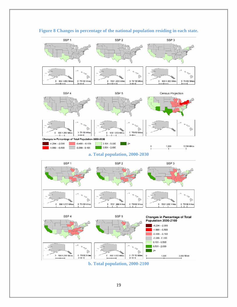
Figure 8 Changes in percentage of the national population residing in each state.

a. Total population, 2000-2030

b. Total population, 2000-2100

19

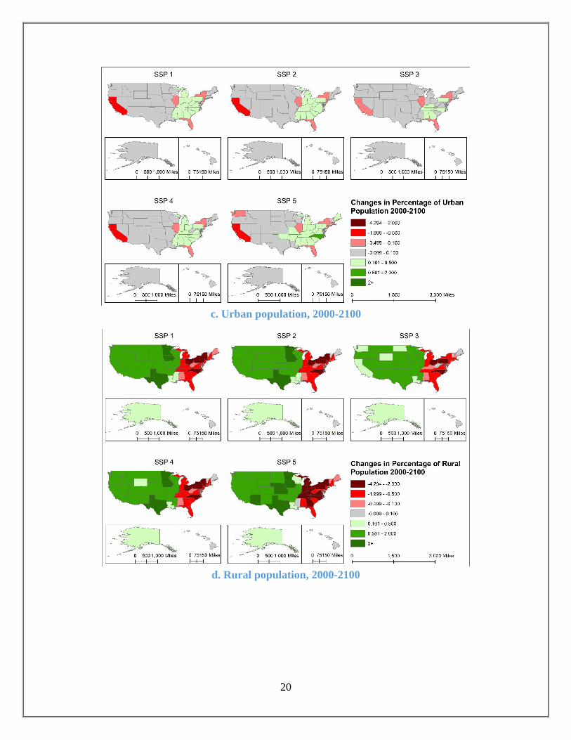
c. Urban population, 2000-2100

d. Rural population, 2000-2100

20

5. Conclusion and Discussion

Consistent projections of US population changes at the national, state, and grid-cell levels are useful for assessing climate change impacts and responses across spatial scales. Within the IM3 project, we are producing a set of national projections carried out at the state level that will ultimately be downscaled to grid cells, providing just such a set of numerically consistent projections across scales. For interim use, we have produced and tested a set of projections that begin with existing spatial population projections based on the Shared Socioeconomic Pathways (SSPs) and upscale them to the state and national level. We tested alternative upscaling methods and resolutions of the SSP spatial projections for their ability to accurately reproduce state and national population totals in the base year, and projected national totals consistent with the SSPs. We also addressed a larger methodological issue: can spatial projections downscaled from the national level directly to grid cells, as was the case for the SSP projections, produce sensible redistributions of population across states?

Our analysis showed that aggregation methods applied to the spatial SSP projections reproduce well data on the total population at the national and state level in the base year (2000), at least when a higher resolution (1 km) version of the spatial projections is used. However, the aggregation of urban and rural populations to the state level is much less accurate (compared to Census data), due not to the aggregation method but to the nature of the underlying spatial population distribution, which was produced as part of the SSP-based spatial projections in a way that defined urban and rural populations differently than in the Census data.

Evaluation of the spatial projections beyond the 2000 base year showed the aggregation of these results reproduces well the original national projections from which they were produced, and that the Census Bureau projection is similar to the SSP2 projection at the national level, through the Census Bureau time horizon of 2030. At the state level, the upscaled outcomes are less consistent with the Census Bureau projections. The Census Bureau projections are generally more consistent with data for actual state population outcomes in 2010, and through 2030 more than half of the Census Bureau state projections fall outside the range of the upscaled SSP-based projections. Moreover, the upscaling outcomes of projected populations by demographic characteristics (urban and rural residence in this study) can be less reliable than the projections of state total populations. This is also due to the fact that the original downscaling method does not

21

explicitly consider the regional variations in future migration flows and urbanization processes.

In general, we conclude that the aggregated state projections of total populations are acceptable for use on an interim basis, based on the comparison to Census data for the years 2000 and 2010 and to the Census Bureau’s state population projections up to the year 2030. However, the results must be used with caution, because the comparison to the state level population projections from the Census Bureau shows that in many states, the spatial projections miss important demographic dynamics, most likely driven by internal migration. Furthermore, the upscaling results for state-level rural and urban population projections are less reliable, especially for the rural population. There is a clear need for explicit state-level projections that can better reflect the consequences of internal migration for sub-national redistribution of the population, and that can reflect urbanization processes consistent with current Census data on the distribution of urban and rural population.

22

References O’Neill, B.C., Kriegler, E., Riahi, K. et al. 2014. A new scenario framework for

climate change research: the concept of shared socioeconomic pathway. Climatic Change 122 (3): 387-400.

Melillo, Jerry M., Terese (T.C.) Richmond, and Gary W. Yohe, Eds., 2014:

Climate Change Impacts in the United States: The Third National Climate Assessment. U.S. Global Change Research Program, 841 pp. doi:10.7930/J0Z31WJ2

Gao, Jing, 2017. Downscaling global spatial population projections from 1/8-

degree to 1-km grid cell. NCAR Technote (forthcoming). Jiang, L. and O’Neill, B.C., 2015. Global urbanization projections for the

Shared Socioeconomic Pathways. Global Environmental Change. Jones, B. and O’Neill, B.C., 2016. Spatially explicit global population

scenarios consistent with the Shared Socioeconomic Pathways. Environmental Research Letters, 11(8), p.084003.

Balk, D.L., U. Deichmann, G. Yetman, F. Pozzi, S. I. Hay, and A. Nelson.

2006. Determining Global Population Distribution: Methods, Applications and Data. Advances in Parasitology 62:119-156.

Perry, M.J. and P.J. Mackun, 2001: Population Change and Distribution –

Census 2000 Brief. US Census Bureau. US Census Bureau, 2005: Interim population projections for states, by age

and sex: 2004 to 2030. Washington DC. Center for International Earth Science Information Network (CIESIN)

Columbia University, United Nations Food and Agriculture Programme (FAO) and Centro Internacional de Agricultura Tropical (CIAT) 2005: Gridded Population of theWorld, Version 3 (GPWv3): Population Count Grid (Palisades, NY: NASA Socioeconomic Data and Applications Center).

23

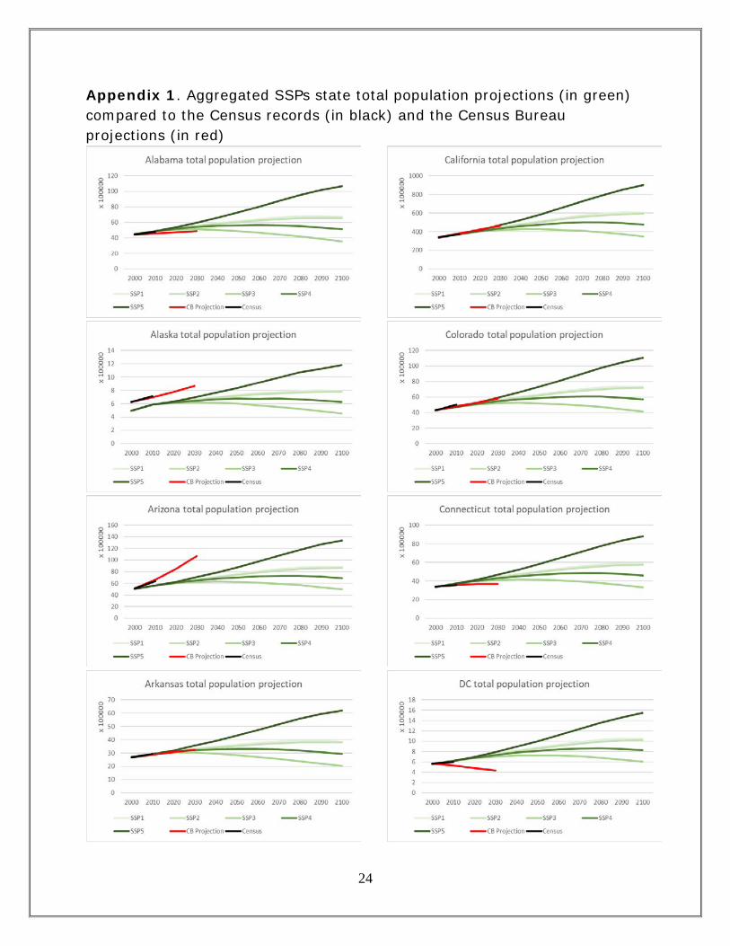
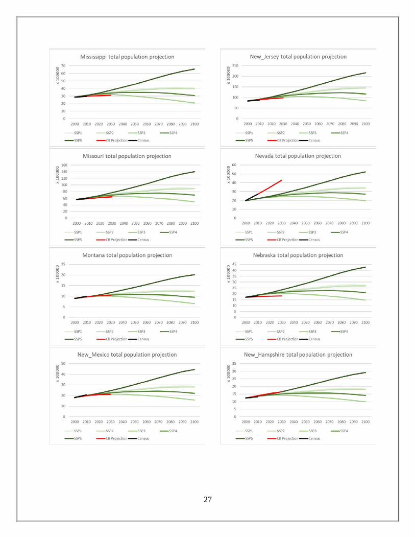
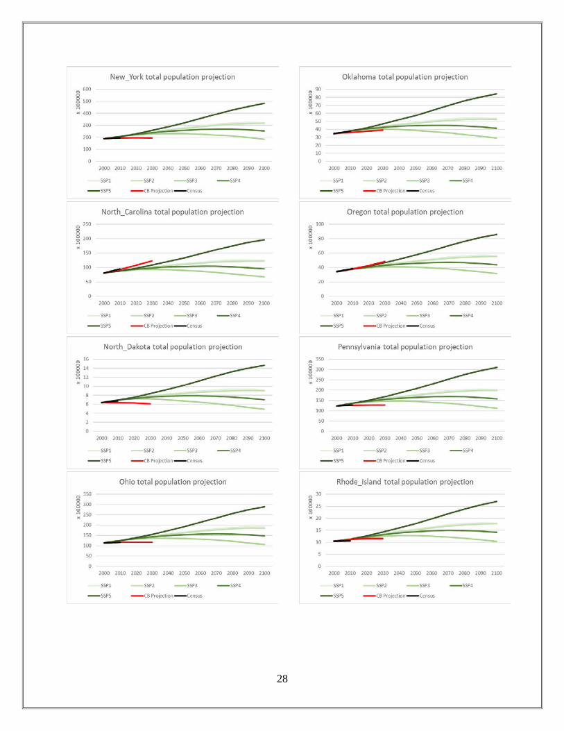
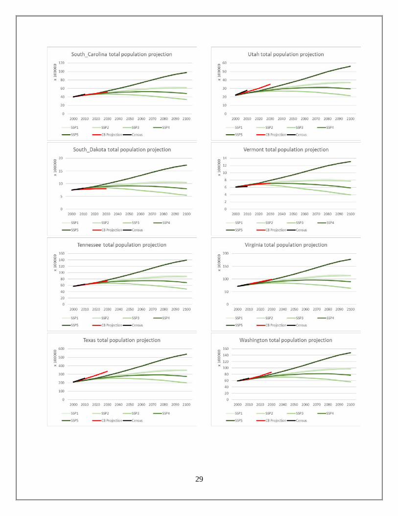
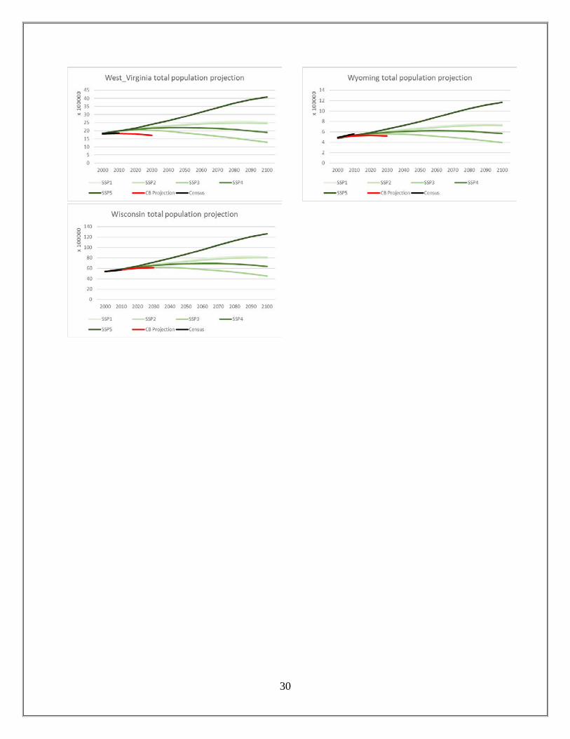
Appendix 1. Aggregated SSPs state total population projections (in green) compared to the Census records (in black) and the Census Bureau projections (in red)

24

25

26

27

28

29

30

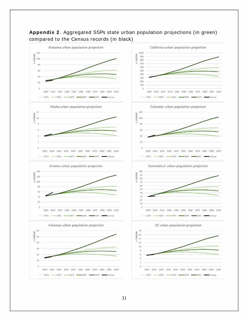
Appendix 2. Aggregated SSPs state urban population projections (in green) compared to the Census records (in black)

31

32

33

34

35

36

37

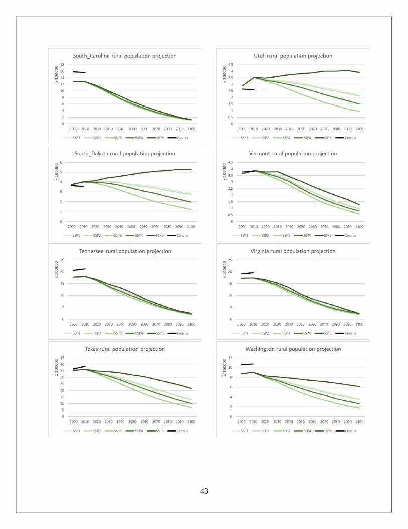
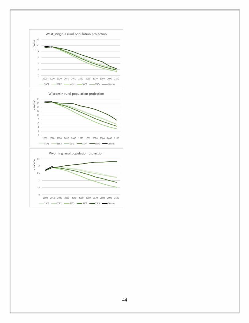
Appendix 3. Aggregated SSPs state rural population projections (in green) compared to the Census records (in black)

38

39

40

41

42

43

44