NCAR/TN- 477+STR

NCAR TECHNICAL NOTE ________________________________________________________________________

February 2010

Scientific Documentation for the NMM Solver

Zavisa Janjic Robert Gall Matthew E. Pyle

Research Applications Laboratory Joint Numerical Testbed

Developmental Testbed Center ________________________________________________________________________

NATIONAL CENTER FOR ATMOSPHERIC RESEARCH P. O. Box 3000

BOULDER, COLORADO 80307-3000 ISSN Print Edition 2153-2397

ISSN Electronic Edition 2153-2400

2

NCAR TECHNICAL NOTES http://www.ucar.edu/library/collections/technotes/technotes.jsp

The Technical Notes series provides an outlet for a variety of NCAR Manuscripts that contribute in specialized ways to the body of scientific knowledge but that are not suitable for journal, monograph, or book publication. Reports in this series are issued by the NCAR scientific divisions. Designation symbols for the series include:

EDD – Engineering, Design, or Development Reports Equipment descriptions, test results, instrumentation, and operating and maintenance manuals. IA – Instructional Aids Instruction manuals, bibliographies, film supplements, and other research or instructional aids. PPR – Program Progress Reports Field program reports, interim and working reports, survey reports, and plans for experiments. PROC – Proceedings Documentation or symposia, colloquia, conferences, workshops, and lectures. (Distribution may be limited to attendees). STR – Scientific and Technical Reports Data compilations, theoretical and numerical investigations, and experimental results.

The National Center for Atmospheric Research (NCAR) is operated by the nonprofit University Corporation for Atmospheric Research (UCAR) under the sponsorship of the National Science Foundation. Any opinions, findings, conclusions, or recommendations expressed in this publication are those of the author(s) and do not necessarily reflect the views of the National Science Foundation.

3

NCAR/TN- 477+STR NCAR TECHNICAL NOTE

________________________________________________________________________

Scientific Documentation for NMM Solver Zavisa Janjic Environmental Modeling Center, National Centers for Environmental Prediction, Camp Springs, MD Robert Gall Development Manager, Hurricane Forecast Improvement Program, NOAA/OST, Silver Spring, MD Matthew E. Pyle Environmental Modeling Center, National Centers for Environmental Prediction, Camp Springs, MD The Developmental Testbed Center (DTC) supported the preparation of this Technical Note. Dr. Robert Gall was the National Director of the DTC and the Director of the Joint Numerical Testbed in NCAR’s Research Applications Laboratory at the time preparations for this document were undertaken.

________________________________________________________________________ NATIONAL CENTER FOR ATMOSPHERIC RESEARCH

P. O. Box 3000 BOULDER, COLORADO 80307-3000

4

TABLE OF CONTENTS

LIST OF FIGURES ........................................................................................................... 6 ACKNOWLEDGMENTS .................................................................................................... 7

1.0 INTRODUCTION ........................................................................................................ 8

1.1 Non-Hydrostatic Mesoscale Model System (NMM) ........................................... 9

1.2 Major features of the NMM system ................................................................. 10

2.0 MODEL EQUATIONS ................................................................................................ 12

2.1 Basic model equations .................................................................................... 12

2.2 The Non-hydrostatic solver ............................................................................ 15

3.0 TEMPORAL DISCRETIZATION ............................................................................... 20

3.1 General philosophy ......................................................................................... 20 3.1.1 Adams-Bashforth time differencing ............................................................20 3.1.2 The Crank-Nicholson differencing scheme ...................................................22 3.1.3 Time integration of the fast adjustment process ..........................................23 3.1.4 Time integration of vertically propagating sound waves ...............................23 3.1.5 Advection of other variables ........................................................................23

3.2 The time discrete equations ........................................................................... 24

3.3 Solution of the coupled equations .................................................................. 27

3.4 Time stepping .................................................................................................. 29

3.5 Computer timing considerations .................................................................... 30

4.0 HORIZONTAL COORDINATE SYSTEM .................................................................. 30

5.0 HORIZONTAL GRID ................................................................................................ 32

5.1 The E-grid ..................................................................................................... 32

5.2 Comments on the choice of the E-grid .......................................................... 34

6.0 HORIZONTAL DISCRETE EQUATIONS ................................................................. 38

6.1 Horizontal advection ........................................................................................ 39

5

6.2 Pressure gradient force .................................................................................. 40

6.3 General comments on conservations properties in the NMM ........................ 42

7.0 VERTICAL COORDINATE AND VERTICAL STAGGERING .................................. 44

8.0 BOUNDARY CONDITIONS ....................................................................................... 47

8.1 Lateral boundary conditions ........................................................................... 47

8.2 Vertical boundary conditions ......................................................................... 47

9.0 TURBULENT MIXING AND MODEL FILTERS ........................................................ 48

9.1 Explicit Lateral Diffusion ................................................................................. 48

9.2 Divergence damping ...................................................................................... 49

10.0 REFERENCES ........................................................................................................ 52

6

List of Figures 1.1 The WRF System. ............................................................................................................ 7 2.1 Parameters of the sigma coordinate system. ............................................................... 111 3.1 Amplification factors for the computational mode (red) and the meteorological mode in

the Adams-Bashforth time differencing scheme. Wave number is shown along the abscissa with the 4 ∆ x wave in the center, the 2 ∆ x wave to the right and infinite wave number on the left. ........................................................................................................ 19

3.2 Same as Figure 3.1 except the amplification factor scale near 1 is amplified. Here the green line shows the amplification factor for the modified Adams-Bashforth scheme, (3.1.1.2). ........................................................................................................................ 20 3.3 Time stepping process in the NMM. The fundamental time step dt=t2-t1 is the time step

for the dynamical process (shown by the red arrows). The time step for passive substance advection is 2 dt as illustrated by the blue arrows. ....................................... 27

4.1 The left hand figure shows a typical domain centered at 38N, 92W plotted on a regular latitude longitude map background. The right hand figure shows the same domain projected on a rotated latitude longitude map background. .......................................... 30

5.1 E-Grid lattice. ................................................................................................................ 31 5.2 Illustration of dx and dy on the E-grid. Conventional grid spacing is the diagonal

distance “d” or the shortest distance between two adjacent grid points where like variables are stored, which in the case of the E-grid is along a diagonal. The grid spacings specified in the model are the dx and dy values. ........................................... 31

5.3 The staggered C-grid and the semi-staggered B-, E- and Z-grids. ................................ 33 5.4 The difference between the Charney-Phillips and the Lorenz vertical staggering. ...... 35 5.5 The ratio νC/f as a function of X and Y. ....................................................................... 36 6.1 An illustration of the E-grid used to define quantities used in Section 6.1.1. ............... 37 6.2 The Z- grid equivalent of the E-grid. Orientations of the coordinate axes x, y and 'x , 'y are indicated. ................................................................................................................. 42 7.1 The hybrid vertical coordinate used in the NMM. ........................................................ 44 8.1 Lateral boundary conditions. H denotes mass variables and V the velocity vector. .... 45 9.1 Stencil of grid points used to compute mass divergence. ............................................. 48

7

Acknowledgments The authors want to thank all who helped prepare the final manuscript. Tom Black, Tom Warner and Yubao Liu carefully reviewed the draft manuscript and provided many comments and suggestions. Ligia Bernardet also reviewed the manuscript and suggested many edits. Carol Makowski provided a final edit of the manuscript and addressed a number of formatting issues. Louisa Nance proofed the revised manuscript and provided some final edits. She handled overseeing the process of submitting document as an NCAR Technical Note.

8

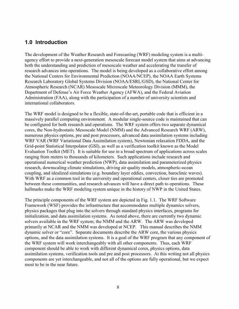
1.0 Introduction The development of the Weather Research and Forecasting (WRF) modeling system is a multi-agency effort to provide a next-generation mesoscale forecast model system that aims at advancing both the understanding and prediction of mesoscale weather and accelerating the transfer of research advances into operations. The model is being developed as a collaborative effort among the National Centers for Environmental Prediction (NOAA/NCEP), the NOAA Earth Systems Research Laboratory Global Systems Division (NOAA/ESRL/GSD), the National Center for Atmospheric Research (NCAR) Mesoscale Microscale Meteorology Division (MMM), the Department of Defense’s Air Force Weather Agency (AFWA), and the Federal Aviation Administration (FAA), along with the participation of a number of university scientists and international collaborators. The WRF model is designed to be a flexible, state-of-the-art, portable code that is efficient in a massively parallel computing environment. A modular single-source code is maintained that can be configured for both research and operations. The WRF system offers two separate dynamical cores, the Non-hydrostatic Mesoscale Model (NMM) and the Advanced Research WRF (ARW), numerous physics options, pre and post processors, advanced data assimilation systems including WRF VAR (WRF Variational Data Assimilation system), Newtonian relaxation FDDA, and the Grid-point Statistical Interpolator (GSI), as well as a verification toolkit known as the Model Evaluation Toolkit (MET). It is suitable for use in a broad spectrum of applications across scales ranging from meters to thousands of kilometers. Such applications include research and operational numerical weather prediction (NWP), data assimilation and parameterized physics research, downscaling climate simulations, driving air quality models, atmospheric-ocean coupling, and idealized simulations (e.g. boundary layer eddies, convection, baroclinic waves). With WRF as a common tool in the university and operational centers, closer ties are promoted between these communities, and research advances will have a direct path to operations. These hallmarks make the WRF modeling system unique in the history of NWP in the United States. The principle components of the WRF system are depicted in Fig. 1.1. The WRF Software Framework (WSF) provides the infrastructure that accommodates multiple dynamics solvers, physics packages that plug into the solvers through standard physics interfaces, programs for initialization, and data assimilation systems. As noted above, there are currently two dynamic solvers available in the WRF system; the NMM and the ARW. The ARW was developed primarily at NCAR and the NMM was developed at NCEP. This manual describes the NMM dynamic solver or “core”. Separate documents describe the ARW core, the various physics options, and the data assimilation systems. It is a goal of the WRF program that any component of the WRF system will work interchangeably with all other components. Thus, each WRF component should be able to work with different dynamical cores, physics options, data assimilation systems, verification tools and pre and post processors. At this writing not all physics components are yet interchangeable, and not all of the options are fully operational, but we expect most to be in the near future.

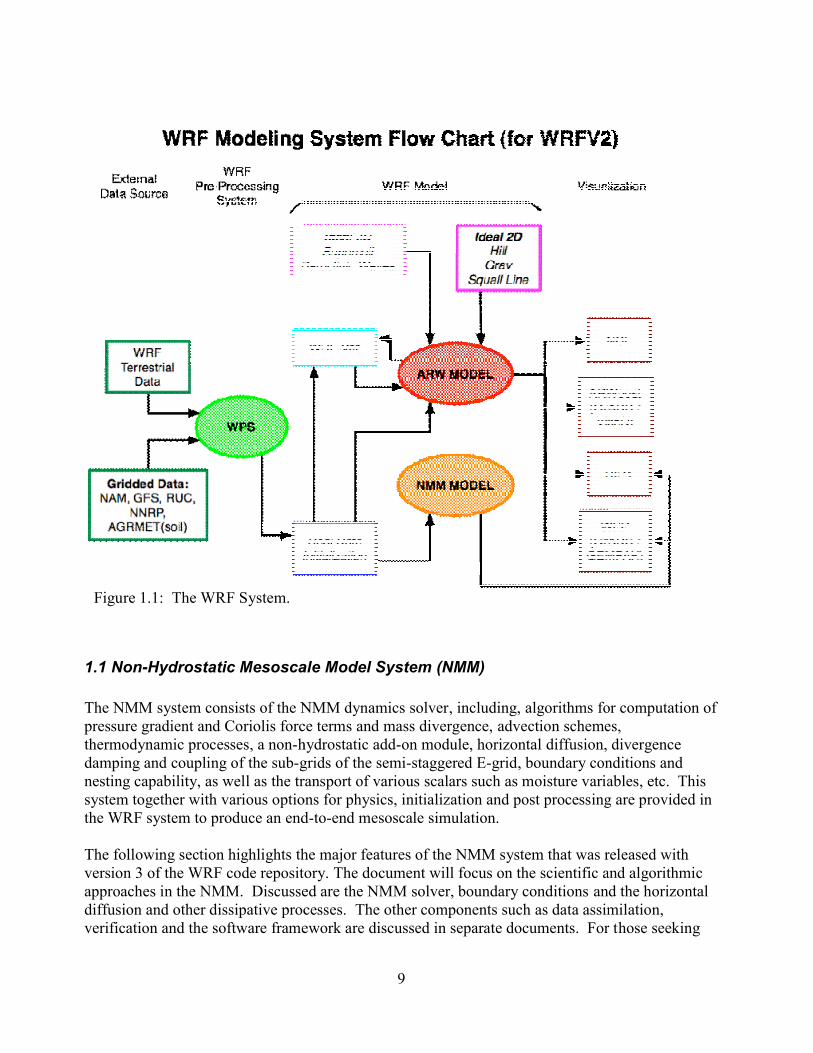
Figure 1. The WRF System

1.1 Non-Hydrostatic Mesoscale Model System (NMM) The NMM system consists of the NMM dynamics solverpressure gradient and Coriolis force terms and mass divergence,thermodynamic processes, a non-hydrostaticdamping and coupling of the sub-grnesting capability, as well as the transport of various system together with various options for physics, initialization and post processing are provided in the WRF system to produce an end The following section highlights the major features of the NMM system that was released with version 3 of the WRF code repository.approaches in the NMM. Discussed are the NMM solver, boundary conditionsdiffusion and other dissipative processes.verification and the software framework are discussed in separate documents. For t

Figure 1.1: The WRF System.

9

Hydrostatic Mesoscale Model System (NMM)

The NMM system consists of the NMM dynamics solver, including, algorithms for computation of pressure gradient and Coriolis force terms and mass divergence, advection schemes

hydrostatic add-on module, horizontal diffusion, divergence grids of the semi-staggered E-grid, boundary conditions and

the transport of various scalars such as moisture variablessystem together with various options for physics, initialization and post processing are provided in

tem to produce an end-to-end mesoscale simulation.

The following section highlights the major features of the NMM system that was released with of the WRF code repository. The document will focus on the scientific and algorithmic

n the NMM. Discussed are the NMM solver, boundary conditions and the horizontal diffusion and other dissipative processes. The other components such as data assimilation, verification and the software framework are discussed in separate documents. For t

algorithms for computation of schemes,

diffusion, divergence , boundary conditions and

such as moisture variables, etc. This system together with various options for physics, initialization and post processing are provided in

The following section highlights the major features of the NMM system that was released with will focus on the scientific and algorithmic

and the horizontal The other components such as data assimilation,

verification and the software framework are discussed in separate documents. For those seeking

10

information on running the NMM modeling system, please refer to the NMM user’s guide (http://www.dtcenter.org/wrf-nmm/users/docs/user_guide/V3/index.pdf).

1.2 Major features of the NMM system A general philosophy was adopted in constructing the NMM core. The NMM:

• Uses modeling principles proven in NWP and regional climate applications.

• Uses numerical methods that control the nonlinear energy cascade and minimize generation of small-scale computational noise.

• Uses full compressible equations split into hydrostatic and non-hydrostatic contributions.

o Easy comparison of hydrostatic and non-hydrostatic solutions. o Reduced computational effort at lower resolutions.

• Robustness and computational efficiency.

With these principles in mind, the characteristics of the NMM solver include: • Equations: Fully compressible, Euler non-hydrostatic with a hydrostatic option.

• Prognostic variables: Horizontal wind components, temperature, non-hydrostatic pressure and

hydrostatic surface pressure, and scalars such as water vapor mixing ratio, rain/snow mixing ratio and cloud water/ice mixing ratio.

• Vertical coordinate: Terrain-following hydrostatic-pressure based sigma coordinate up to a specified pressure surface usually below the tropopause, and hydrostatic pressure coordinate above. Top of the model is a constant pressure surface.

• Horizontal coordinate: Rotated latitude-longitude.

• Vertical grid: Lorenz staggering. • Horizontal grid: Arakawa E-grid staggering.

• Time integration: Forward-backward for fast waves, implicit for vertically propagating sound

waves, Adams-Bashforth for horizontal advection and Coriolis terms, Crank-Nicholson for vertical advection, and Lagrangian upstream passive substance advection with forced conservation, positive definiteness and monotonization (an option for tracer advection).

• Spatial discretization: Conserves mass, momentum, energy, enstrophy (for nondivergent flow) and a number of other quadratic quantities.

11

• Lateral turbulent mixing and model filters: Smagorinsky nonlinear lateral diffusion,

divergence damping and coupling of the sub grids of the semi-staggered E-grid by modifying the divergence term in the mass continuity equation (see 5.2).

• Initial conditions: Can be derived from a variety of sources including interpolation from existing grids, and various data assimilation systems.

• Lateral boundary conditions: Specified from a larger domain model.

• Top boundary conditions: Vertical velocity in the pressure coordinate system at the top boundary (a constant pressure level) is zero; non-hydrostatic pressure is equal to hydrostatic pressure. No special filtering is applied near the top boundary.

• Bottom boundary conditions: Vertical velocity in the sigma coordinate is set to zero, vertical derivative of the difference between the non-hydrostatic and hydrostatic pressures is zero. Boundary conditions for model’s physics are specified by land surface and surface layer schemes.

• Earth’s rotation: Coriolis terms included.

The following physics parameterizations are available: • Microphysics: Bulk schemes ranging from simplified physics suitable for mesoscale

modeling to sophisticated mixed-phase physics for cloud resolving models.

• Cumulus Parameterizations: Adjustment and mass-flux schemes. • Surface physics: Multi-layer surface models ranging from a simple thermal model to full

vegetation and soil moisture models, including snow cover and sea ice.

• Planetary boundary layer and free atmosphere turbulence physics: Similarity theory surface layer schemes, turbulent kinetic energy prediction and non-local schemes.

• Atmospheric radiation: Longwave and shortwave schemes with multiple spectral bands and

a simple shortwave scheme. Cloud effects and surface fluxes are included. The NMM may be initialized from:

• WRF VAR (http://www.mmm.ucar.edu/wrf/users/wrfda/index.html) • GSI (http:/www.dtcenter.org/com-GSI/users).

• WRF Pre-processing System (WPS)

12

2.0 Model equations Considerable experience has been accumulated in the formulation and application of non-hydrostatic models on cloud or single storm scales. However, NWP deals with motions on a much wider range of temporal and spatial scales. Difficulties that may not be significant, or may go unnoticed on the mesoscale, could spoil a forecast on the synoptic scale. For example, an erratic gain or loss of mass would be hard to tolerate in an operational environment where the absence of such errors with highly evolved NWP models is taken for granted. Another problem may arise regarding the control of spurious motions generated in upper levels by the non-hydrostatic dynamics and numerics. Forcing the variables at the top model layers toward a constant basic state in time appears to be inadequate in NWP applications. On the other hand, time-dependent computational top boundary conditions could limit the ability of a regional non-hydrostatic model to produce synoptic scale forecasts more accurate than the parent hydrostatic model. Finally, there is insufficient experience concerning the benefits of non-hydrostatic models that can be expected in NWP. For these reasons, a non-hydrostatic NWP model must be fully competitive with mature hydrostatic models in the range of validity of the hydrostatic approximation. Of course, the model should be able to reproduce non-hydrostatic motions at very high resolutions in order to demonstrate the soundness of the formulation. Another obvious requirement is that the extra computational effort due to the more complex non-hydrostatic dynamics be modest. Having in mind these criteria, a new approach has been proposed (Janjic et al. 2001, Janjic 2003) as an alternative to the usual methods of extending mesoscale non-hydrostatic modeling concepts to the synoptic scales. This approach is based on relaxing the hydrostatic approximation in a hydrostatic model using a vertical coordinate based on hydrostatic pressure, and thus extending the applicability of the model to non-hydrostatic motions. The system of non-hydrostatic equations was split into two parts: (a) the part that corresponds to the hydrostatic system, and (b) corrections to the hydrostatic system due to the vertical acceleration. The separation of the non-hydrostatic contributions shows in a transparent way how the hydrostatic approximation affects the equations. This procedure does not require any linearization or additional approximation. At the same time, the favorable features of the hydrostatic model are preserved within the range of validity of the hydrostatic approximation. The non-hydrostatic dynamics has been introduced through an add-on module in the NCEP NMM model (Janjic et al. 2001). The non-hydrostatic module can be turned on and off depending on resolution. This allows easy comparison of hydrostatic and non-hydrostatic solutions obtained using otherwise identical models. The basic philosophy behind the discretization methods applied in the model is reviewed in the next section.

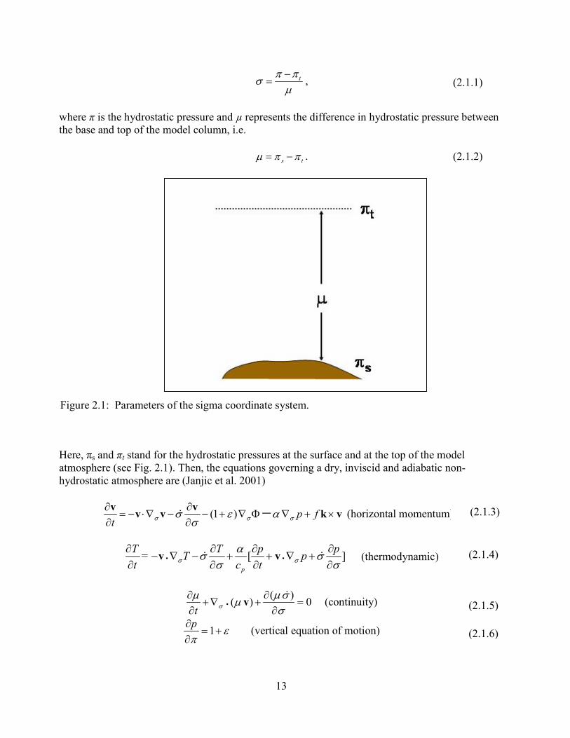
2.1 Basic model equations For simplicity, consider the sigma vertical coordinate as the simplest and most popular representative of terrain following coordinates (Fig. 2.1)

13

tπ πσµ−

= ,

where π is the hydrostatic pressure and µ represents the difference in hydrostatic pressure between the base and top of the model column, i.e.

s tµ π π= − .

Here, πs and πt stand for the hydrostatic pressures at the surface and at the top of the model atmosphere (see Fig. 2.1). Then, the equations governing a dry, inviscid and adiabatic non-hydrostatic atmosphere are (Janjic et al. 2001)

(1 ) p ft σ σ σσ ε α

σ∂ ∂

= − ⋅∇ − − + ∇ Φ ∇ + ×∂ ∂

−v vv v k v (horizontal momentum) )

[ ]p

T T p p= T pt c tσ σ

ασ σσ σ

• •∂ ∂ ∂ ∂

− ∇ − + + ∇ +∂ ∂ ∂ ∂

v v

(thermodynamic)

( )( ) 0

t σµ µσµ

σ•

∂ ∂+∇ + =

∂ ∂v

(continuity)

1p επ∂

= +∂

(vertical equation of motion)

Figure 2.1: Parameters of the sigma coordinate system.

(2.1.1)

(2.1.1)

(2.1.2)

(2.1.3)

(2.1.4)

(2.1.5)

(2.1.6)

(2.1.3)

(2.1.4)

(2.1.5) (2.1.5) (2.1.5)

(2.1.6)

14

RTp

µσ∂Φ

= −∂

(hypsometric)

1 1 ( )σ

dw σg dt g t σ

•Φ ∂Φ ∂Φ

= = + ∇ Φ+∂ ∂

v (non-hydrostatic continuity)

RT pα = (equation of state)

1 dwg dt

ε ≡ (definition of ε)

Here, in the order of appearance, v is the horizontal wind vector, p is the non-hydrostatic pressure, R is the gas constant for dry air, T is temperature, and Φ is geopotential. The other symbols used have either their usual meaning, or their meaning is self-evident. Note that the non-hydrostatic continuity equation (2.1.8) and the definition of ε (2.1.10) are not independent equations. The parameter ε is the central point of the extended, non-hydrostatic dynamics. As can be readily verified, if ε is zero, (2.1.3)–(2.1.7) reduce to the familiar, hydrostatic equations. The additional equations (2.1.6), (2.1.8) and (2.1.10) are needed in order to compute the corrections due to nonzero ε. The presence of nonzero ε demonstrates in a very transparent way where, how, and to what extent relaxing the hydrostatic approximation affects the familiar hydrostatic equations. Note that the system of equations developed above bears a close relation to the system discussed by Laprise (1992). Note:

• Φ , w, ε are not independent and there is no independent prognostic equation for w! Instead, w is computed diagnostically from the non-hydrostatic continuity equation.

• ε <<1 in meso and large scale atmospheric flows.

• The impact of non-hydrostatic dynamics becomes detectable at scales < 10 km, and

important at 1 km.

The NMM predicted variables are:

o Mass variables: PD – Time and space varying component of the hydrostatic surface

pressure (Pa) PINT – non-hydrostatic pressure (Pa) T – sensible temperature (K) Q – specific humidity (kg/kg) CWM – total cloud water condensate (kg/kg). Higher order microphysics

schemes will have more moisture variables. q2 – 2 * turbulent kinetic energy (m2 s-2)

(2.1.7)

(2.1.8)

(2.1.9)

(2.1.10)

(2.1.7)

(2.1.8)

(2.1.9)

(2.1.10)

15

o Wind variables: u,v – wind components (m s-1)

Note: q2 is calculated using the Mellor, Yamada, Janjic scheme (Janjic 2001) as part of the NMM physics package. It is used in the calculation of the horizontal mixing. Physics package components are not discussed in this technical note.

2.2 The Non-hydrostatic solver The method of solving the system of non-hydrostatic equations (2.1.3)–(2.1.10) is presented in detail in the paper by Janjic et al (2001). Assume that a box with cross section S contains a mass of air M with the density ρ. Then,

Mg S g S zµ σ ρ= ∆ = ∆ ,

where g is gravity and z∆ is the height of the box. The hypsometric equation that relates the geopotential Φ to the hydrostatic pressure,

α µσ∂Φ

= −∂

,

is readily obtained from (2.2.1). In (2.2.2), α is the non-hydrostatic specific volume. Using the definitions of σ and μ , (2.2.2) may be rewritten as

απ∂Φ

= −∂

.

Assuming that the atmosphere is dry, the specific volume is related to the temperature T and pressure p by the ideal gas law, pRT=α . Note that the ideal gas law does not involve the hydrostatic pressure but rather the actual pressure. Using the ideal gas law, from (2.2.2)

RTp

µσ∂Φ

= −∂

.

Upon integration of (2.2.4) from the surface, where the surface geopotential is denoted by sΦ , to an arbitrary level σ ,

1

sσ

RTΦ Φ μ dσp

= + ∫ .

Using (2.2.3), the third equation of motion may be written as

(2.2.1)

(2.2.2)

(2.2.3)

(2.2.4)

(2.2.5)

16

1( )dw pgdt π

∂= −

∂.

Defining the ratio of the vertical acceleration and gravity as,

1 dwg dt

ε ≡ ,

(2.2.6) may be rewritten as

1p επ∂

= +∂

,

which defines the relationship between the hydrostatic and the non-hydrostatic pressures. Integrating (2.2.8) with respect to π, one obtains the non-hydrostatic pressure at an arbitrary hydrostatic pressure or σ level, i.e,

0

(1 )t

pp d dπ σ

π

π ε µ σπ∂ ′ ′= = +′∂∫ ∫ .

As can be seen from (2.2.8) and (2.2.9), should ε vanish, the pressure and the hydrostatic pressure become equivalent. In the hydrostatic σ coordinate system, the time derivative of a fluid property q following the motion of an air parcel may be written as

σqσq

tq

dtdq

σ ∂∂

+∇+∂∂

= • v ,

where σ is the vertical velocity. The conservation of mass may be expressed by

1 ( )σw σg t σ

•∂Φ ∂Φ

= + ∇ Φ +∂ ∂

v ,

and, if μ is substituted for σπ ∂∂ , then

0σdμ σμdt σ

•∂ + ∇ + = ∂

v .

(2.2.6)

(2.2.9)

(2.2.10)

(2.2.11)

(2.2.7)

(2.2.8)

(2.2.12)

17

Equation (2.2.11) may be regarded as a definition of w, the time rate of change of geopotential height following the motion of a fluid parcel. Equation (2.2.12) is the mass continuity equation in the form used in hydrostatic models. Using the material surface boundary conditions 0=≡ dtdσσ at 0=σ and 1=σ , one may obtain two equations from (2.2.12). The first one gives the tendency of the hydrostatic surface pressure

1

0

( ) dt σµ µ σ•∂ ′= − ∇∂ ∫ v ,

and the second one is used to calculate the vertical velocity in the σ coordinate system

0

( ) dt

σ

σµµσ σ µ σ•∂ ′= − − ∇∂ ∫ v .

Using the relations (2.2.3) and (2.2.8), in the case of a non-hydrostatic atmosphere one obtains

1 (1 )z p pσ σε αρ

− ∇ − + ∇ Φ ∇≡ − .

Here the subscripts indicate the variable that is kept constant while the differentiation is performed. Using (2.2.15), the inviscid non-hydrostatic equation for the horizontal part of the wind takes the form

(1 )d p fdt σ σε α= − + ∇ Φ ∇ + ×−v k v .

Again, for vanishing ε , (2.2.16) reduces to the form used in hydrostatic models. The first law of thermodynamics for adiabatic processes has the form

pdpdTc dt dt

α=

in which pc is the specific heat at constant pressure. In hydrostatic models, the derivative dtdp

is replaced by the derivative of hydrostatic pressure dtdπ , often denoted by the Greek letter omega ���. For this reason, the right hand side of the equation is frequently referred to as the “omega–alpha” term. The derivative of pressure can be separated into a component 1ω , which

reduces to the hydrostatic expression when ε vanishes, and a component 2ω , which vanishes with vanishing ε . Note that, generally )t,,y,x(pp π= . Then

(2.2.13)

(2.2.14)

(2.2.15)

(2.2.16)

(2.2.17)

18

(1 )t

p p p pt t t t tπ π

π πεπ

∂ ∂ ∂ ∂ ∂ ∂= + = + +

∂ ∂ ∂ ∂ ∂ ∂,

where the subscripts indicate the variable that is kept constant while the differentiation is performed. In addition to that, as can be seen from (2.2.8),

(1 )p πσ ε σσ σ∂ ∂

= +∂ ∂

.

Thus, dtdp is written in the form

1 2dpdt

ω ω= + ,

where

1 (1 ) (1 )pt σπ πω ε ε σ

σ•

∂ ∂≡ + + ∇ + +

∂ ∂v ,

or taking into account (2.2.14) and the fact that σπμ ∂∂= ,

10

(1 ) ( )p dσ

σ σω ε µ σ• • ′= ∇ − + ∇∫v v .

Note that the contribution of the second term of the pressure gradient force (2.2.15) to the kinetic energy generation is compensated by the contribution of the horizontal advection of pressure in (2.2.21). The second part of ω is defined by

2 (1 )pt t

πω ε∂ ∂≡ − +∂ ∂

.

Starting from (2.2.12), it can be shown that

σ ε σ µ σ µ εω δσ

τ σ τ σ2

0

′ ′∂ ∂( ) ∂( ) ∂ ′= −∫ ′ ′∂ ∂ ∂ ∂[ ] .

Note that the term (2.2.23) vanishes for vanishing ε . In view of the separation of omega into two parts, the thermodynamic equation is separated into two parts as well;

(2.2.18)

(2.2.19)

(2.2.20)

(2.2.21)

(2.2.22)

(2.2.23)

(2.2.24)

19

11 ( )1( )

p

T T= Tt cσ σ αω

σ•

∂ ∂− ∇ − +

∂ ∂v

and

21 ( )2( )

p

T =t c

αω∂∂

.

Note that with the aid of (2.2.22), (2.2.25) may be rewritten as

0

[ (1 ) ( ) ]1( )p

T T= T p dt c

σ

σ σ σασ ε µ σ

σ• • •

∂ ∂ ′− ∇ − + ∇ − + ∇∂ ∂ ∫v v v .

Again, when ε vanishes, (2.2.25) and (2.2.27) take the form used in hydrostatic models, and the equation for the second part (2.2.26) takes the trivial form 02 =∂∂ )tT( . The non-hydrostatic system of equations is closed by applying the operator (2.2.10) to the continuity equation (2.2.11) in order to obtain the vertical acceleration dtdw . Then, from (2.2.7),

1 1 ( )σdw w ww σ

g dt g t σε •

∂ ∂= = + ∇ +

∂ ∂v .

On the synoptic scales, ε is very small and approaches the computer round–off error. However, in case of vigorous convective storms, or strong vertical accelerations in the flows over steep obstacles, the vertical velocity can reach the order of 10 m s-1 over a period of the order of 1000 s. This yields an estimate of the vertical acceleration of the order of 2 210 m s− − , and consequently, ε

of the order of 310− . As can be seen from (2.2.8), for this value of ε the non-hydrostatic deviations of pressure can reach 100 Pa. Bearing in mind that the typical synoptic scale horizontal pressure gradient is of the order of 100 Pa over 100 km, this suggests that significant local non-hydrostatic pressure gradients and associated circulations may develop on small scales. Nevertheless ε remains much smaller than 1 in atmospheric flows, and therefore, the non-hydrostatic effects in (2.1.3)–(2.1.10) are of a higher-order magnitude. An important consequence of this situation for the discretization is that high accuracy of computation of ε does not appear to be of paramount importance, since the computational errors are of even higher order than ε itself.

(2.2.25-) (2.2.25)

(2.2.26)

(2.2.27)

(2.2.28)

20

3.0 Temporal discretization

3.1 General philosophy The general philosophy for the time integration in the NMM is:

• Explicit where possible for accuracy, computational efficiency and coding transparency:

horizontal advection of u, v, and T. advection of various other variables such as water vapor mixing ratio (q), cloud

water, and turbulent kinetic energy (TKE). adjustment terms

• Implicit for very fast processes that would require a restrictively short time step for

numerical stability with explicit differencing:

vertical advection and vertically propagating sound waves. For the basic dynamic variables, the NMM uses four types of time integration: (i) modified Adams-Bashforth, for horizontal advection of u,v, and T, and Coriolis terms, (ii) Crank Nicholson for vertical advection of u,v, and T, (iii) forward-backward scheme for adjustment terms and (iv) an implicit scheme for vertically propagating sound waves.

3.1.1 Adams-Bashforth time differencing The Adams-Bashforth scheme can be represented as:

113 1( ) ( )

Δ 2 2y y f y f y

t

τ ττ τ

+−−

= − .

Note that this method has a slight linear instability, which can be tolerated in practice or stabilized by slight off-centering as is done in the WRF-NMM:

111.533 ( ) 0.533 ( )

Δy y f y f y

t

τ ττ τ

+−−

= − .

Figure 3.1 shows the amplification of the meteorological mode (green) and the computational mode (red) for 3.1.1.1. The plot is for linear one-dimensional centered second order advection with constant advection speed of 110 m s-1 and a time step equal to one third of the maximum allowed time step by the Courant–Friedrichs–Lewy (CFL) criterion. Here wave number is plotted on the x

(3.1.1.2)

(3.1.1.1)

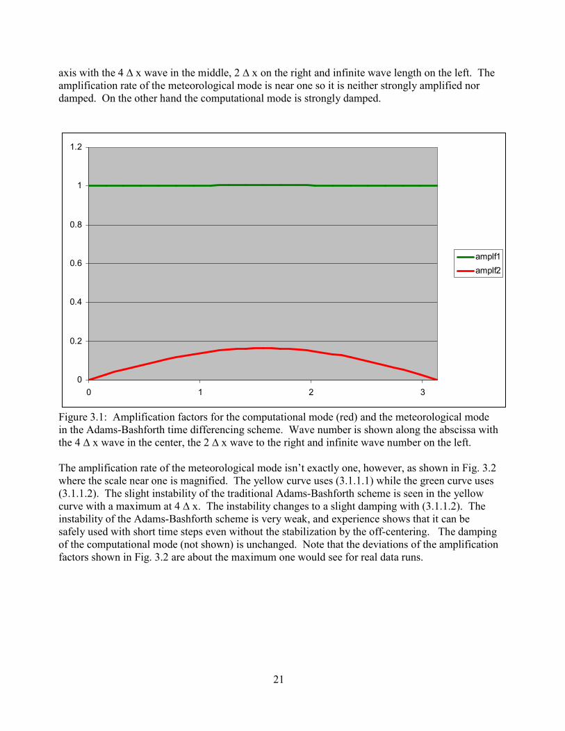
21

axis with the 4 ∆ x wave in the middle, 2 ∆ x on the right and infinite wave length on the left. The amplification rate of the meteorological mode is near one so it is neither strongly amplified nor damped. On the other hand the computational mode is strongly damped.

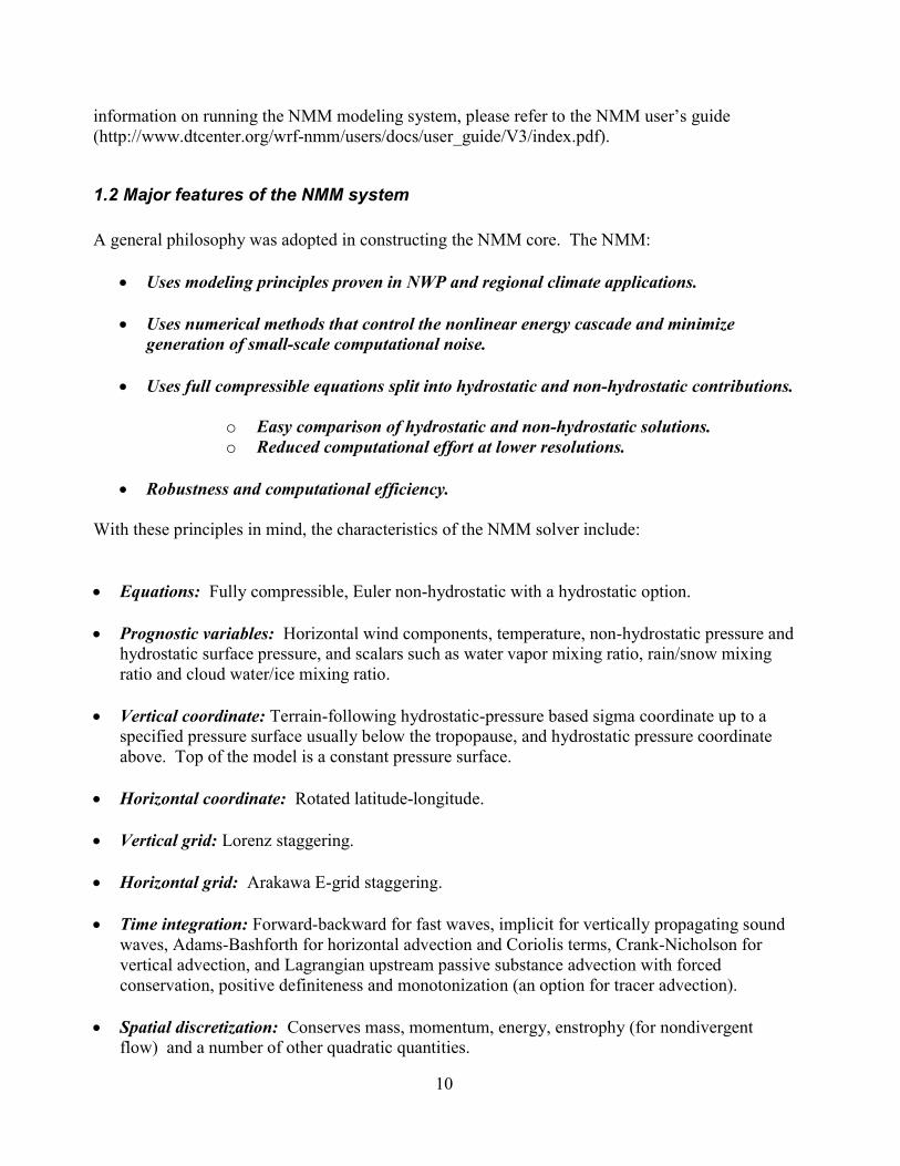
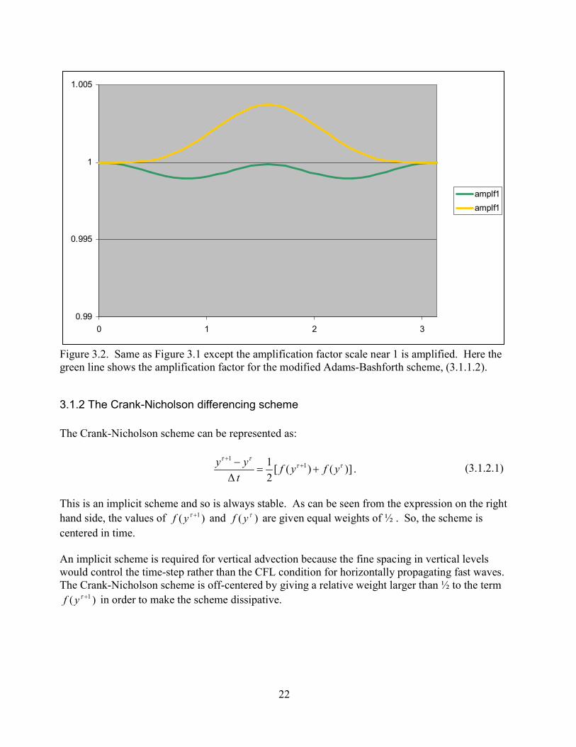
Figure 3.1: Amplification factors for the computational mode (red) and the meteorological mode in the Adams-Bashforth time differencing scheme. Wave number is shown along the abscissa with the 4 ∆ x wave in the center, the 2 ∆ x wave to the right and infinite wave number on the left. The amplification rate of the meteorological mode isn’t exactly one, however, as shown in Fig. 3.2 where the scale near one is magnified. The yellow curve uses (3.1.1.1) while the green curve uses (3.1.1.2). The slight instability of the traditional Adams-Bashforth scheme is seen in the yellow curve with a maximum at 4 ∆ x. The instability changes to a slight damping with (3.1.1.2). The instability of the Adams-Bashforth scheme is very weak, and experience shows that it can be safely used with short time steps even without the stabilization by the off-centering. The damping of the computational mode (not shown) is unchanged. Note that the deviations of the amplification factors shown in Fig. 3.2 are about the maximum one would see for real data runs.

0

0.2

0.4

0.6

0.8

1

1.2

0 1 2 3

amplf1amplf2

22

Figure 3.2. Same as Figure 3.1 except the amplification factor scale near 1 is amplified. Here the green line shows the amplification factor for the modified Adams-Bashforth scheme, (3.1.1.2).

3.1.2 The Crank-Nicholson differencing scheme The Crank-Nicholson scheme can be represented as:

111 [ ( ) ( )]

Δ 2y y f y f y

t

τ ττ τ

++−

= + .

This is an implicit scheme and so is always stable. As can be seen from the expression on the right hand side, the values of )( 1+τyf and )( τyf are given equal weights of ½ . So, the scheme is centered in time. An implicit scheme is required for vertical advection because the fine spacing in vertical levels would control the time-step rather than the CFL condition for horizontally propagating fast waves. The Crank-Nicholson scheme is off-centered by giving a relative weight larger than ½ to the term

)( 1+τyf in order to make the scheme dissipative.

0.99

0.995

1

1.005

0 1 2 3

amplf1amplf1

(3.1.2.1)

23

3.1.3 Time integration of the fast adjustment process Time integration of terms involving the propagation of gravity waves is handled by a forward-backward process (Ames 1969; Gadd 1974; Janjic and Wiin-Nielsen 1977; Janjic 1979; Mesinger 1977). Using the shallow water equations to illustrate the process:

. The mass tendency equation is advanced by a forward step:

. The velocity equations are then advanced with a backward step:

.

3.1.4 Time integration of vertically propagating sound waves The time integration of vertically propagating sound waves is hidden inside the implicit algorithm used to solve the full model equations. Details of this calculation are found in section 3.3. However, if the model equations were linearized, the following wave equation can be derived for non-hydrostatic pressure (Janjic et al. 2001) where � ' represents a perturbation pressure. This equation is given here only as an illustration. It is not used in the model.

3.1.5 Advection of other variables The scheme for advecting any other variable such as water vapor and liquid water uses the very basic upstream Lagrangian forward time differencing, which can be represented in one dimension by:

1*1 , 0j j j jy y y y

u ut x

τ τ τ τ+−− −

= − >∆ ∆

.

This is followed by a negative diffusion step to reduce smoothing:

,u h h u

g Ht x t x

∂ ∂ ∂ ∂= − = −

∂ ∂ ∂ ∂

1 Δu

h h t Hx

ττ τ ∂+ = −

∂

11 Δ .h

u u t gx

ττ τ

++ ∂= −

∂

2 1 1 2 1

02 2 20

' ' ' '2n n n np

v

cp p p p pRTt t c z

+ − +′∂ − + ∂= =

∂ ∆ ∂

(3.1.3.1)

(3.1.3.2)

(3.1.3.3)

(3.1.4.1)

(3.1.5.1)

24

1 1* 1* 1* 1*1 1

2

2( ) , ( ) 0j j j j jy y y y yu t u tf f

t x x x

τ τ τ τ τ+ + + + +− +− − +∆ ∆

= − >∆ ∆ ∆ ∆

.

The function f is chosen to minimize computational dispersion in sheared flows. Finally, for all passive quantities conservation is enforced after each anti-diffusion step to maintain the global sum of the quantity, and prevent generation of new extrema. Conservation is achieved by requiring that the sums of positive and negative contributions of the negative diffusion be equal in absolute value. Due to open boundary conditions, the total mass of tracers cannot be conserved by this method.

3.2 The time discrete equations This section provides considerable detail of the time discrete equations that have been outlined in section 3.1. It is intended for readers who wish to work through the actual equations solved by the NMM core. The basics are outlined above so readers not wishing this much detail can skip to the next section. The numerical model described here uses the equations discussed in Section 2.0 cast into finite difference form. Note that, as before, for simplicity, the sigma coordinate is used as a representative of mass based vertical coordinates. The modifications needed for the vertical coordinate actually used in the model are straightforward. By using numerical methods that have been successful in hydrostatic models, it is expected that the model will behave well in the hydrostatic limit, i.e., when applied with resolutions that do not support significant vertical accelerations. For vanishing ε , the prognostic equations of the quasi–hydrostatic system of equations, i.e., (2.2.3), (2.2.12), (2.2.16) and (2.2.27), together with the ideal gas law, can be conveniently split into two energy conserving subsystems of prognostic equations, i.e.,

( ) fit σ σα π∂= −∇ Φ ∇ + ×

∂−v k v

0

[ ( ) ]( )p

T = dit c

σ

σ σα π µ σ• •

∂ ′∇ − ∇∂ ∫v v

( )( ) 0σ

μ σt σ

µµ•∂ ∂

+∇ + =∂ ∂

v

( ) =iit σ σσ

•∂ ∂

− ∇ −∂ ∂v vv v

( )T T= Tiit σ σσ

•∂ ∂

− ∇ −∂ ∂

v

(3.2.1)

(3.2.2)

(3.2.3)

(3.2.4)

(3.2.5)

25

The time derivatives of the two subsystems are denoted by subscripts i and ii, respectively. As can be readily verified, the system (3.2.1)–(3.2.2), together with the continuity equation (2.2.12) rewritten here in somewhat different form (3.2.3), conserves energy. The same applies to the system (3.2.4)–(3.2.5) combined with the continuity equation that links the two subsystems. Note that large ratios between the advection time step, and the time step used for the remaining terms of the equations can not be used in NWP applications. Namely, since the wind speed can exceed 100

1m s− , this ratio is restricted to 2 or 3, at most. The time differencing schemes are applied to the system (2.2.12), (2.2.16) and (2.2.27). The superscripts n and n+1 will be used to denote the time levels for all variables with the exception of the vertical velocity w, which is defined at the intermediate time levels indicated by superscripts n+1/2 or n-1/2. The superscript n+1/2 will be used also in the advection terms in order to indicate the terms extrapolated in time in the Adams–Bashforth procedure. Because the non-hydrostatic equations have been separated into two components, the subscript 1 will be used to indicate that a variable has been advanced in time only by the first component equation. For example, the solution of (2.2.27) starting from the time level n will be denoted by the subscript 1, since (2.2.26) remains to be solved before reaching the time–level n+1. As usual, the vertical velocity in the hydrostatic sigma coordinate is computed from

1

0 0

( ) ( )n n n n

nn

d dσ

σ σσ µ σ µ σσ

µ

• •′ ′∇ − ∇=∫ ∫v v

,

and the surface pressure tendency equation is

11

0

( )n n n nt dσµ µ µ σ•+ ′= − ∆ ∇∫ v .

From the solution for μ 1+n , one readily obtains

11 (1 )( )n n n np p σ ε µ µ+= + + − ,

and

10

(1 ) ( )n n n n np dσ

σ σω ε µ σ• • ′= ∇ − + ∇∫v v .

After adding the Crank-Nicholson vertical, and Adams–Bashforth horizontal advection, one obtains

(3.2.6)

(3.2.7)

(3.2.8)

(3.2.9)

26

)(21

21*1 σ

σ∆ σ ∂∂

+∇−=+

+•

nnnnn T

TtTT v ,

and finally

1*

11 ω∆n

n

p pRT

ctTT += .

The superscript n+1/2 in the advection terms indicates symbolically the extrapolation in time for slightly more than half the time step, 0.533 (see section 3.1.1) involved in the Adams–Bashforth procedure, or averaging in time in the Crank-Nicholson algorithm. The second component of the thermodynamic equation is

)pp(p

RTc

TT n

p

n1

1

1

11

1 1−=− ++ .

The hypsometric equation yields the geopotential associated with the first component solutions for temperature and pressure,

11 1

11

'ns

RT dpσ

µ σ+Φ = Φ + ∫

and the second component equation yields

1 11 1

1 'n

n ns n

RT dpσ

µ σ+

+ ++Φ = Φ + ∫ .

The value of vertical velocity w associated with the first component solutions is obtained from

1 11 1

nn ng w

t σ σσ

•Φ −Φ ∂Φ

= + ∇ Φ +∆ ∂

v .

Note that 1Φ is an intermediate value of geopotential between nΦ and 1+nΦ , i.e.,

11 ( )n O t+Φ −Φ ≤ ∆ .

Therefore, using 1Φ in the advection terms of (3.2.15) in order to compute w is a consistent numerical approximation. On the other hand, neglecting the contribution 1

1( )n t+Φ −Φ ∆ would be wrong in view of (3.2.16). Thus,

(3.2.10)

(3.2.13)

(3.2.14)

(3.2.15)

(3.2.16)

(3.2.11)

(3.2.12)

27

11 2 1

1

nnw w

g t

++ Φ −Φ

− =∆

,

which must also satisfy the vertical equation of motion,

11 2

1 11 (1 )n

nn

g t pw w g t εµ σ

++

+

∆ ∂− = − ∆ +

∂.

The value of ε associated with the first component solutions is gotten from

1 11 1

nn nw w wg w

t σε σσ

•− ∂

= + ∇ +∆ ∂

v ,

and the second component from

11

1

1 1n

nn

pεµ σ

++

+

∂= −

∂.

Upon solution of the preceding equations for thermodynamic variables, the pressure gradient force at the time level n+1 can be computed, and the horizontal equation of motion can be used to advance the wind components in time. The Crank-Nicholson scheme is used for the vertical advection terms, while the modified Adams–Bashforth scheme is used to compute the contribution of the Coriolis force terms and the horizontal advection terms

])([ 2121

21*1 ++

++ ×+∂

∂+∇∆−= •

nn

nnnnn ft vkvvvvvσ

σσ .

Then the backward scheme for the pressure gradient force term is used to complete the step

])1[( 1111*11 ++++++ ∇∇+−= − nnnnnn pt σσ αΦε∆vv . Here, the specific volume 1+nα is

1

11

+

++ = n

nn

pRTα .

3.3 Solution of the coupled equations Eqs. (3.2.12), (3.2.14), (3.2.17) and (3.2.18) are coupled equations. Their solution will be sought by eliminating all unknowns except 1+np , solving the resulting equation, and then back–

(3.2.17)

(3.2.19)

(3.2.21)

(3.2.22)

(3.2.23)

(3.2.18)

(3.2.20)

28

substituting to obtain 1+nT , 1+nΦ , 21+nw and 1+nε . Namely, (3.2.13) and (3.2.14), together with (3.2.17) and (3.2.18), can be combined to give

1 1 11 21

11 11

1( ) [ (1 )]( )n n

nn n

TT pR d g tp pσ

µ σ εµ σ

+ ++

+ +

∂′− = ∆ − +∂∫ .

Using (3.2.12) to eliminate 1+nT , (3.3.1) may be rewritten as

1 11 2

1 11 11

1 1 1(1 ) ( ) [ (1 )]( )n

nn n

pR T d g tp pσ

κ µ σ εµ σ

++

+ +

∂′− − = ∆ − +∂∫

where pcR≡κ . Define a pressure *p that satisfies the equation

*1

1(1 )np µ εσ

+∂≡ +

∂

subject to the boundary condition tp π=* at .0=σ Upon inserting (3.3.3) into (3.3.2), one obtains

1 *

1 1 1 1 12

12 11

(1 )( )

( )n

n n n n

n

p pR T d t

g p pσ

κ µ µ µ µσσ

+

+ + + +

+

∂ −− ′− = ∆

∂∫ .

Note that

1 *

1 1 ( )n

n n

p p O tµ µ

+

+ +− ≤ ∆ ,

so that, from (3.3.4),

1 1 13

12 11

(1 ) ( )( )n n

n

R T d O tg p pσ

κ µ µ σ+ +

+

− ′− ≤ ∆∫ ,

which illustrates how subtle the difference is between 1p and 1+np . Differentiating (3.3.4) with respect to σ , introducing the definitions

1

1

n

n

pψµ

+

+≡ , *

*1n

pψµ +≡ , 1

1 1n

pψµ +≡ , 1

2(1 )( )

RTg t

κΓ ≡ −∆

and rearranging the resulting equation, one obtains

(3.3.1)

(3.3.2)

(3.3.3)

(3.3.4)

(3.3.5)

(3.3.6)

(3.3.7)

29

*2 *

12

1

( ) 0ψ ψψ ψσ ψ ψ

−∂ −+ Γ =

∂.

Finally, define

*χ ψ ψ≡ − , *1D ψ ψ≡ − and

11 1( ) ( ) [ ( ) ( )]d dψψ σ ψ σ κ ψ σ σ σ ψ σ

σ∂

≡ + − + −∂

.

The product ψψ1 that appears in the denominator of the undifferentiated term in (3.3.8) may be

approximated by 2ψ . Letting 2 2γ ψ≡ Γ , (3.3.8) can then be rewritten as

22 2

2 Dχ γ χ γσ∂

− = −∂

.

The variable χ is set to zero at 0=σ , and 0=∂∂ σχ at 1=σ . Such an upper boundary condition is perfectly justified for vanishing pressure at the top of the atmosphere of the model. As a tridiagonal system, (3.3.10) is solved directly.

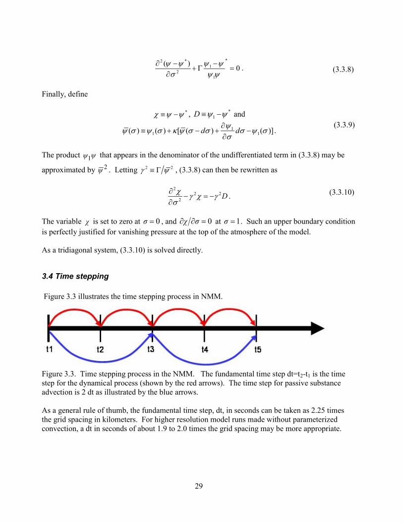
3.4 Time stepping Figure 3.3 illustrates the time stepping process in NMM.

Figure 3.3. Time stepping process in the NMM. The fundamental time step dt=t2-t1 is the time step for the dynamical process (shown by the red arrows). The time step for passive substance advection is 2 dt as illustrated by the blue arrows. As a general rule of thumb, the fundamental time step, dt, in seconds can be taken as 2.25 times the grid spacing in kilometers. For higher resolution model runs made without parameterized convection, a dt in seconds of about 1.9 to 2.0 times the grid spacing may be more appropriate.

(3.3.8)

(3.3.10)

(3.3.9)

30

3.5 Computer timing considerations The list below shows the main subroutines in the time stepping loop of the NMM core. The numbers in parentheses indicate the total approximate time spent in each of these routines in terms of the total amount of time spent in the time stepping loop. The calculations in some of these routines are described in later sections.

• (0.6%) PDTE – integrates mass flux divergence, computes vertical velocity and updated pressure field.

• (26.4%) ADVE – horizontal and vertical advection of T, u, v, Coriolis and curvature terms applied.

• (1.2%) VTOA – updates non-hydrostatic pressure, applies omega alpha term to thermodynamic equation.

• (8.6%) VADZ/HADZ – vertical/horizontal advection of height. w=dz/dt updated.

• (10.6%) EPS – vertical and horizontal advection of dz/dt, vertical sound wave treatment.

• (19.5%) VAD2/HAD2 (every other step) – vertical/horizontal advection of q, CWM,

TKE.

• (11.8%) HDIFF – horizontal diffusion.

• (1.2%) BOCOH – boundary update at mass points.

• (17.5%) PFDHT – calculates pressure gradient force (PGF), updates winds due to PGF, and computes divergence.

• (2.3%) DDAMP – divergence damping.

• (0.3%) BOCOV – boundary update at wind points.

4.0 Horizontal coordinate system In order to achieve higher computational efficiency of the model code, a transformed latitude-longitude coordinate system has been used. This system is obtained by rotation of the natural, geodesic latitude-longitude in such a way that the intersection of the equator and zero meridian of the transformed system ( 0 0,λ ϕ ) coincides with the center of the model domain. The transformed system provides a more uniform horizontal grid spacing by reducing to a large extent the meridian convergence, and accordingly, allowing the use of a larger time step for the model time

31

integration. The transformation and inverse transformation equations between the rotated and the natural latitude-longitude system ( ,λ ϕ ) are as follows:

( )( ) ϕϕλλϕϕ

λλϕsinsincoscoscos

sincosarctan

000

0

+−−

=Λ

( )( )Φ = − −arcsin cos sin sin cos cosϕ ϕ ϕ ϕ λ λ0 0 0 and

( )ϕ ϕ ϕ= +arcsin sin cos cos cos sin0 0Φ Λ Φ

λ λϕ

= +

0

0

arcsin sin coscosΛ Φ

.

The horizontal wind in the rotated system ( )V = U,V expressed in terms of the wind in the natural latitude/longitude system ( )v = u,v is defined as:

( )[ ] ( )( )[ ]

Uu v

=+ − − −

− − −

cos cos sin sin cos sin sin

cos sin sin cos cos

ϕ ϕ ϕ ϕ λ λ ϕ λ λ

ϕ ϕ ϕ ϕ λ λ

0 0 0 0 0

0 0 02

1

and

( ) ( )[ ]( )[ ]

Vu v

=− + + −

− − −

sin sin cos cos sin sin cos

cos sin sin cos cos

ϕ λ λ ϕ ϕ ϕ ϕ λ λ

ϕ ϕ ϕ ϕ λ λ

0 0 0 0 0

0 0 02

1 .

The inverse wind transformation is given by:

( )( )

uU V

=− +

− +

cos cos sin sin cos sin sin

cos sin sin cos cos

ϕ ϕ ϕ

ϕ ϕ

0 0 0

0 021

Φ Φ Λ Λ

Φ Λ Φ

( )

( )v

U V=− + −

− +

sin sin cos cos sin sin cos

cos sin sin cos cos

ϕ ϕ ϕ

ϕ ϕ

0 0 0

0 021

Λ Φ Φ Λ

Φ Λ Φ.

(4.1)

(4.2)

(4.3)

(4.4)

(4.5)

(4.6)

(4.7)

(4.8)

32

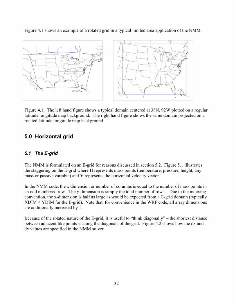
Figure 4.1 shows an example of a rotated grid in a typical limited area application of the NMM.

Figure 4.1. The left hand figure shows a typical domain centered at 38N, 92W plotted on a regular latitude longitude map background. The right hand figure shows the same domain projected on a rotated latitude longitude map background.

5.0 Horizontal grid

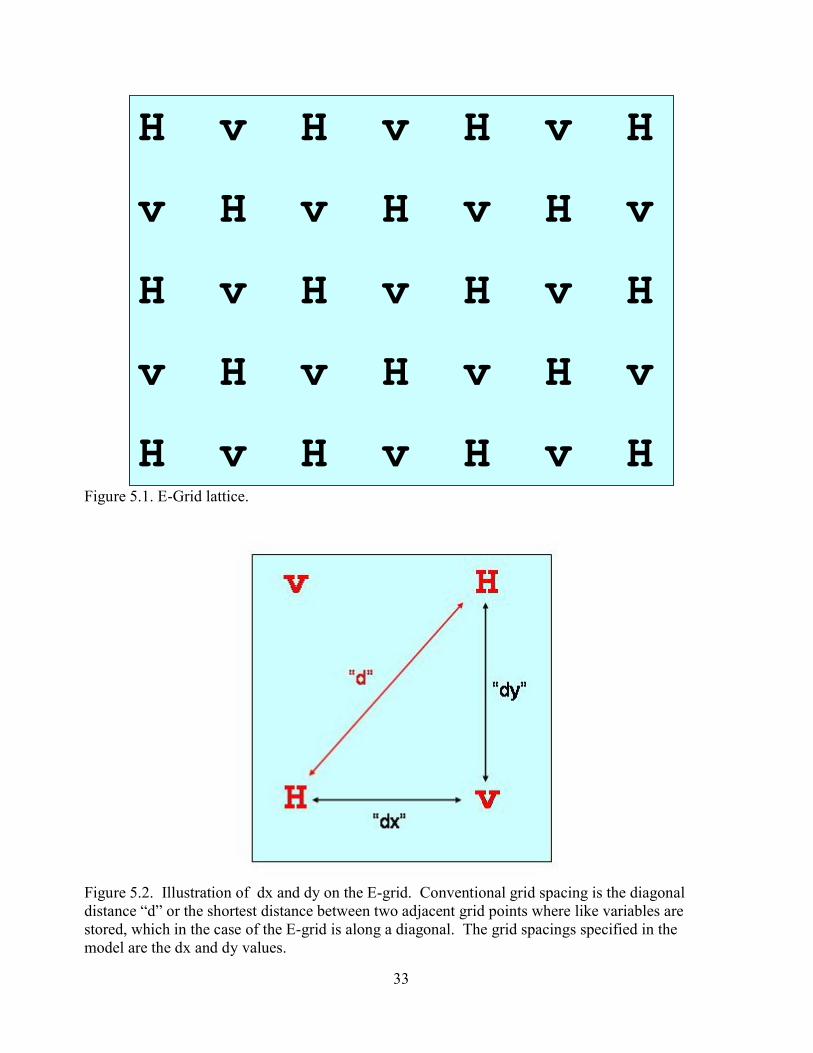
5.1 The E-grid The NMM is formulated on an E-grid for reasons discussed in section 5.2. Figure 5.1 illustrates the staggering on the E-grid where H represents mass points (temperature, pressure, height, any mass or passive variable) and V represents the horizontal velocity vector. In the NMM code, the x dimension or number of columns is equal to the number of mass points in an odd numbered row. The y-dimension is simply the total number of rows. Due to the indexing convention, the x-dimension is half as large as would be expected from a C-grid domain (typically XDIM < YDIM for the E-grid). Note that, for convenience in the WRF code, all array dimensions are additionally increased by 1. Because of the rotated nature of the E-grid, it is useful to “think diagonally” – the shortest distance between adjacent like points is along the diagonals of the grid. Figure 5.2 shows how the dx and dy values are specified in the NMM solver.

33

Figure 5.1. E-Grid lattice.

Figure 5.2. Illustration of dx and dy on the E-grid. Conventional grid spacing is the diagonal distance “d” or the shortest distance between two adjacent grid points where like variables are stored, which in the case of the E-grid is along a diagonal. The grid spacings specified in the model are the dx and dy values.

H v H v H v H

v H v H v H v

H v H v H v H

v H v H v H v

H v H v H v H

34

5.2 Comments on the choice of the E-grid

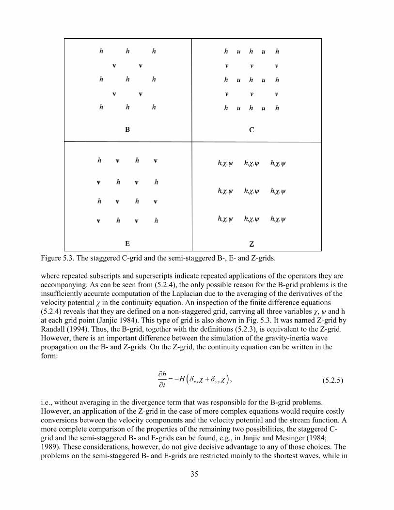
Winninghoff (1968), and Arakawa and Lamb (1977) examined the frequencies of gravity-inertia waves obtained using second-order centered differences on various types of rectangular horizontal grids. According to these studies, compared to other grids considered, generally better agreements with the exact frequencies were obtained on the staggered C-grid, and on the semi-staggered B-grid (or E) shown in Fig. 5.3. The symbol h in the figure denotes the mass point variables, while the horizontal velocity vector and the velocity components are denoted, respectively, by v, u and v. However, the staggered grid and the semi-staggered grids are not without problems, either. The problems on the staggered grid arise due to the averaging of the velocity components in the Coriolis force terms. In order to illustrate the problems on the semi-staggered grids, consider the shallow water equations

, , .u h v h h u vg fv g fu Ht x t y t x y

∂ ∂ ∂ ∂ ∂ ∂ ∂= − + = − − = − + ∂ ∂ ∂ ∂ ∂ ∂ ∂

Here, u and v are the velocity components, h is the height of the free surface, g is gravity, f is the Coriolis parameter assumed to be constant, and H is the mean depth of the fluid. The other symbols used have their usual meaning. The system (5.2.1) discretized in the most straightforward way, e.g., on the B-grid, has the form:

( ), ,y x y x

x y x yu v hg h fv g h fu H u vt t t

δ δ δ δ∂ ∂ ∂= − + = − − = − +

∂ ∂ ∂.

In Eq. (5.2.2), the symbol δ and the over bar, respectively, represent the simplest two-point centered differencing and averaging operators applied in the direction indicated by the accompanying subscript or superscript. Following Janjic (1984), the velocity components on the B-grid may be written in terms of the velocity potential χ and the stream function ψ in the form:

,y x x y

x y y xu vδ χ δ ψ δ χ δ ψ= − = + . Then, after substituting the expressions (5.2.3) into the system (5.2.2), and rearranging, one obtains

( ), ,y y x x

x x y yhgh f f H

t t tχ ψψ χ δ χ δ χ∂ ∂ ∂= − + = − = − +

∂ ∂ ∂

(5.2.1)

(5.2.2)

(5.2.3)

(5.2.4)

35

Figure 5.3. The staggered C-grid and the semi-staggered B-, E- and Z-grids. where repeated subscripts and superscripts indicate repeated applications of the operators they are accompanying. As can be seen from (5.2.4), the only possible reason for the B-grid problems is the insufficiently accurate computation of the Laplacian due to the averaging of the derivatives of the velocity potential χ in the continuity equation. An inspection of the finite difference equations (5.2.4) reveals that they are defined on a non-staggered grid, carrying all three variables χ, ψ and h at each grid point (Janjic 1984). This type of grid is also shown in Fig. 5.3. It was named Z-grid by Randall (1994). Thus, the B-grid, together with the definitions (5.2.3), is equivalent to the Z-grid. However, there is an important difference between the simulation of the gravity-inertia wave propagation on the B- and Z-grids. On the Z-grid, the continuity equation can be written in the form:

( )x x y yh Ht

δ χ δ χ∂= − +

∂,

i.e., without averaging in the divergence term that was responsible for the B-grid problems. However, an application of the Z-grid in the case of more complex equations would require costly conversions between the velocity components and the velocity potential and the stream function. A more complete comparison of the properties of the remaining two possibilities, the staggered C-grid and the semi-staggered B- and E-grids can be found, e.g., in Janjic and Mesinger (1984; 1989). These considerations, however, do not give decisive advantage to any of those choices. The problems on the semi-staggered B- and E-grids are restricted mainly to the shortest waves, while in

(5.2.5)

36

the case of the slow internal modes, and/or weak stability, the C-grid may develop problems in the entire range of the admissible wave numbers (cf. Arakawa and Lamb, 1977). In addition, there is an effective technique for filtering the low frequency, short-wave noise resulting from the inaccurate computation of the divergence term on the semi-staggered grids (Janjic 1979). More sophisticated, non-dissipative methods (‘‘deaveraging’’ and ‘‘isotropisation’’) for dealing with the problem also have been proposed (Janjic et al. 1998), leading to dramatic improvements of the finite difference frequencies of the short gravity-inertia waves on the semi-staggered grids. These techniques are not implemented in the WRF NMM because the improvement in the finite difference frequencies would require significant reduction of the time step allowed for linear stability, and thus the computational efficiency of the model would be reduced. On the other hand, in practice, the B/E grid problem is hardly visible in high resolution runs, so that the sacrifice of the computational efficiency would not be warranted by noticeable forecast improvements. The results discussed so far are relevant for classical synoptic scale model design. In order to address the question of the choice of the horizontal grid as the mesoscales are approached, consider the linearized anelastic non-hydrostatic system

2

, ,

, 0

u P v P w Pfv fut x t y t z

u v wN wt x y z

θ

θ

∂ ∂ ∂ ∂ ∂ ∂= − + = − − = − +

∂ ∂ ∂ ∂ ∂ ∂∂ ∂ ∂ ∂

= − + + =∂ ∂ ∂ ∂

Here, ( )' '

0 0 0, ,pP c gθ π θ θ θ θ= = is the basic state potential temperature, π′ is the Exner function perturbation, θ′ is the potential temperature perturbation and N is the Brunt-Vaisala frequency. Assuming, as usual, the solutions of the form

( )0

i kx ly mzA A e + += ,

where A stands for any dependent variable appearing in (5.2.6), k, l, and m are the wave numbers in the directions of the coordinate axes x, y and z, and ν is the frequency, the frequency equation may be written in the form

( )2

2 2 22

2 2 2

N k l mf

f k l mν

+ + = + +

.

Defining for brevity X=kd, Y=ld, Z=mΔz, where d is the horizontal distance between two nearest points carrying the same variable, and Δz is the vertical grid size, (5.2.8) can be rewritten as

(5.2.7)

(5.2.8)

(5.2.6)

37

( )2

2 2 22

22 2 2

N dX Y Zf z

f dX Y Zz

ν + + ∆ =

+ + ∆

.

The normalized frequencies on the B– and C-grids, respectively, are (communicated by Klemp)

2 22 2 2 2 2 2

2

2 2 22 2 2 2 2

cos cos sin cos sin sin2 2 2 2 2 2

cos sin cos sin sin2 2 2 2 2

B

N Z Y X X Y d zf z

f Y X X Y d Zz

ν+ +

∆=

+ +∆

,

and

2 22 2 2 2 2 2

2

2 22 2 2

cos sin sin cos cos sin2 2 2 2 2 2

sin sin sin2 2

C

N Z X Y d X Y Zf z

f X Y d Zd z

ν+ +

∆=

+ +∆

.

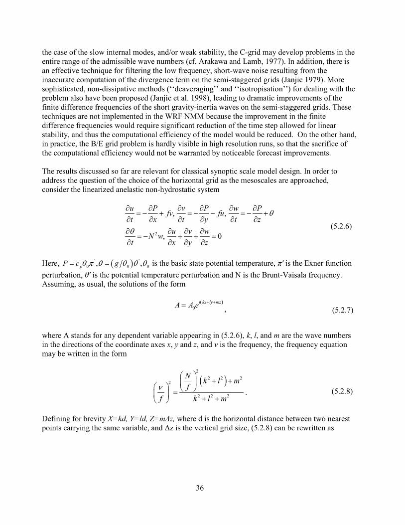
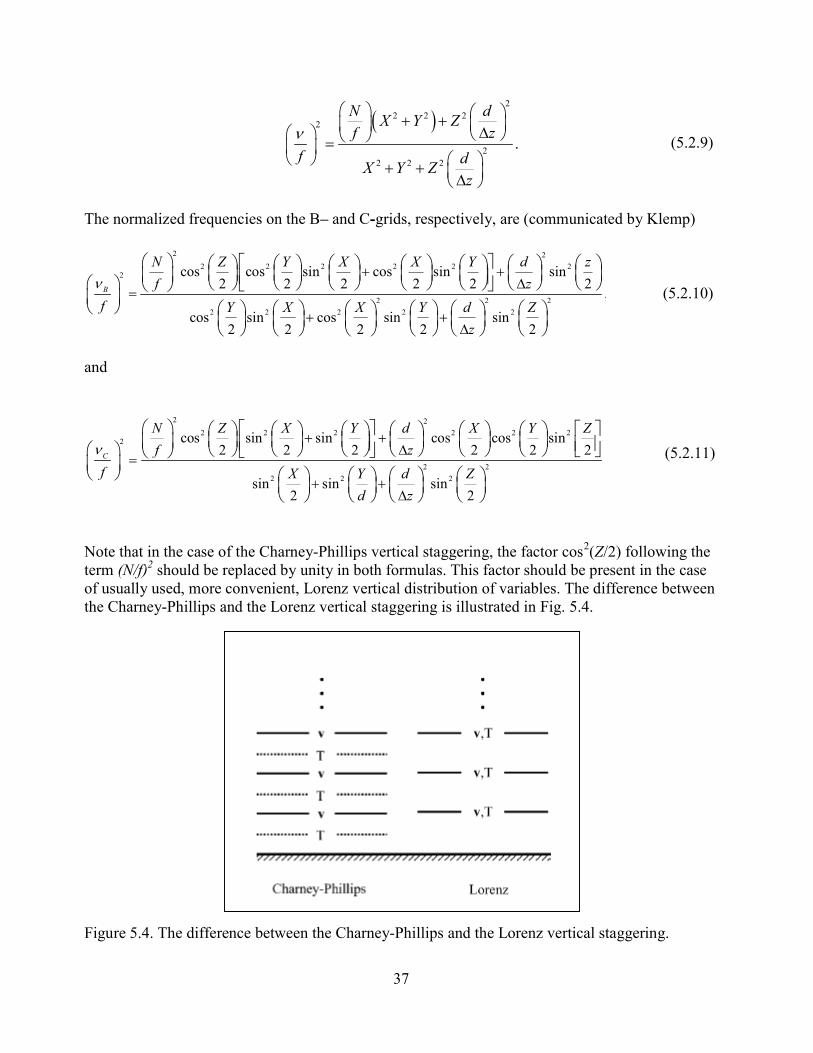
Note that in the case of the Charney-Phillips vertical staggering, the factor cos2(Z/2) following the term (N/f)2 should be replaced by unity in both formulas. This factor should be present in the case of usually used, more convenient, Lorenz vertical distribution of variables. The difference between the Charney-Phillips and the Lorenz vertical staggering is illustrated in Fig. 5.4.

Figure 5.4. The difference between the Charney-Phillips and the Lorenz vertical staggering.

(5.2.10)

(5.2.11)

(5.2.9)

38

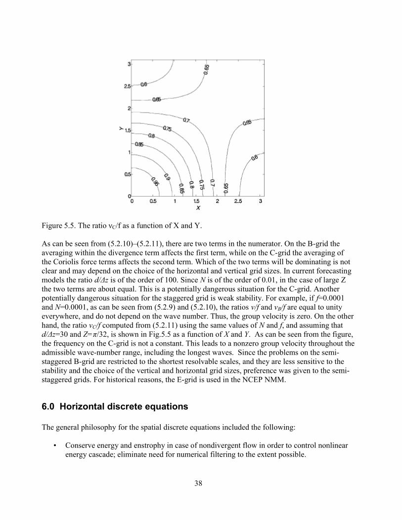
Figure 5.5. The ratio νC/f as a function of X and Y. As can be seen from (5.2.10)–(5.2.11), there are two terms in the numerator. On the B-grid the averaging within the divergence term affects the first term, while on the C-grid the averaging of the Coriolis force terms affects the second term. Which of the two terms will be dominating is not clear and may depend on the choice of the horizontal and vertical grid sizes. In current forecasting models the ratio d/Δz is of the order of 100. Since N is of the order of 0.01, in the case of large Z the two terms are about equal. This is a potentially dangerous situation for the C-grid. Another potentially dangerous situation for the staggered grid is weak stability. For example, if f=0.0001 and N=0.0001, as can be seen from (5.2.9) and (5.2.10), the ratios ν/f and νB/f are equal to unity everywhere, and do not depend on the wave number. Thus, the group velocity is zero. On the other hand, the ratio νC/f computed from (5.2.11) using the same values of N and f, and assuming that d/Δz=30 and Z=π/32, is shown in Fig.5.5 as a function of X and Y. As can be seen from the figure, the frequency on the C-grid is not a constant. This leads to a nonzero group velocity throughout the admissible wave-number range, including the longest waves. Since the problems on the semi-staggered B-grid are restricted to the shortest resolvable scales, and they are less sensitive to the stability and the choice of the vertical and horizontal grid sizes, preference was given to the semi-staggered grids. For historical reasons, the E-grid is used in the NCEP NMM.

6.0 Horizontal discrete equations The general philosophy for the spatial discrete equations included the following:

• Conserve energy and enstrophy in case of nondivergent flow in order to control nonlinear energy cascade; eliminate need for numerical filtering to the extent possible.

39

• Use consistent formulations and order of accuracy for advection and divergence operators. • Energy conserving form of the omega-alpha term; consistent transformations between

kinetic energy (KE) and potential energy (PE). • Conserve a number of first order and quadratic quantities, such as momentum and advected

quantities.

• Reproduce in finite-difference operators certain properties of differential operators.

• Minimize the errors due to presence of topography.

ϕ

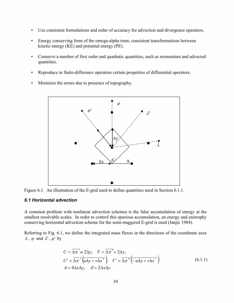
Figure 6.1. An illustration of the E-grid used to define quantities used in Section 6.1.1.

6.1 Horizontal advection A common problem with nonlinear advection schemes is the false accumulation of energy at the smallest resolvable scales. In order to control this spurious accumulation, an energy and enstrophy conserving horizontal advection scheme for the semi-staggered E-grid is used (Janjic 1984). Referring to Fig. 6.1, we define the integrated mass fluxes in the directions of the coordinate axes λ , ϕ and 'λ , 'ϕ by

( ) ( )yxAyxA

xvyuVxvyuU

xvVyuU

∆∆=∆∆=∆+∆−∆=′∆+∆∆=′

∆∆=∆∆=

2',4,

,2,2'''' λϕϕλ

ϕλ

ππ

ππ

'ϕ

λ

∆x A A’

∆y

'λ

(6.1.1)

40

where π∆ is the thickness of the layer in hydrostatic pressure and

ϕ∆∆λ∆ϕ∆ ayax == ,)cos( . Then we can write for the horizontal advection of T, u and v:

( ) ( )' '

' '1 1 1 2 1 ' ' ...

3 3 'T U T V T U T V Tt A A

λ ϕ λ ϕ

λ ϕ λ ϕ∂∂ π

= − ∆ + ∆ + ∆ + ∆ + ∆

...'

1321

311 '

'

'

' +

′+′+

+−=

ϕ

ϕλλ

λλϕ

ϕλλ

λλ

λ ∆∆∆∆π∆∂

∂ uVuUA

uVuUAt

u

...'

1321

311 '

'

'

' +

′+′+

+−=

ϕ

ϕϕλ

λϕϕ

ϕϕλ

λϕ

ϕ ∆∆∆∆π∆∂

∂ vVvUA

vVvUAt

v

6.2 Pressure gradient force Using the definitions in section 6.1, the mass (hydrostatic) continuity equation can be written as follows: For the sigma range:

( ) ( ) ( )σµ∆∆∆∆∆∂π∆∂

σϕλϕλ −

′+′++−= VU

AVU

At '''1

321

31

.

For the pressure range:

( ) ( ) ω∆∆∆∆∆ πϕλϕλ −

′+′++−= VU

AVU

A '''1

321

310 ,

and for the interface between the sigma and pressure ranges

( ) II ωσµ = . The pressure gradient force components are:

Φ∆ε λλ

λ ''

' )1( +=P ,

(6.1.2)

(6.1.3)

(6.1.4)

(6.2.1)

(6.2.3)

(6.2.4)

(6.2.2)

(6.2.3)

(6.2.4)

41

Φ∆επ∆ λλλ

λ '''

' )1( +=PP ,

σλ

λ

σλ ∆ pp

cqRTC '

'

')1608.0(

+−= ,

σλ

λ

σλ

λ ∆π∆ pp

cqRTPC '

''

')1608.0(

+−= ,

Φ∆ε ϕϕ

ϕ ''

' )1( +=P ,

Φ∆επ∆ ϕϕϕ

ϕ '''

' )1( +=PP ,

σϕ

ϕ

σϕ ∆ pp

cqRTC '

'

')1608.0(

+−= ,

σϕ

ϕ

σϕ

ϕ ∆π∆ pp

cqRTPC '

''

')1608.0(

+−= ,

−=

''

''2

1 λϕ

φλλ PPP ,

−=

''

''2

1 λϕ

φλλ PPPPPP ,

−=

''

''2

1 λϕ

φλλ CCC ,

−=

''

''2

1 λϕ

φλλ PCPCPC ,

+=

''

''2

1 λϕ

φλϕ PPP ,

+=

''

''2

1 λϕ

φλϕ PPPPPP ,

+=

''

''2

1 λϕ

φλϕ CCC ,

+=

''

''2

1 λϕ

φλϕ PCPCPC .

(6.2.6)

(6.2.7)

(6.2.8)

(6.2.9)

(6.2.10)

(6.2.11)

(6.2.12)

(6.2.13)

(6.2.16)

(6.2.17)

(6.2.18)

(6.2.19)

(6.2.5)

(6.2.14)

(6.2.15)

(6.2.16)

(6.2.18)

(6.2.19)

(6.2.9)

(6.2.10)

(6.2.12)

42

The pressure gradient force is given by:

...)(132)(

31

21

+

+++−=

∂∂

λλλλλπ∆∆

PCPPCPxt

u ,

and

...)(132)(

31

21

+

+++−=

∂∂

ϕϕϕϕϕπ∆∆

PCPPCPyt

v .

The horizontal advection part of the omega-alpha term is:

( )' '

' '

' '

1 1 2 231 1 ...

2 1 ( ) ( )3 '

py

u yPC v yPCAT

t c u y v x PC u v x PCA

λ φ

λ φ

λ φφ λ

λ φ

∂∂ π

∆ + ∆ = − + ∆ + ∆ + ∆ + − ∆ + ∆

6.3 General comments on conservations properties in the NMM

The conservation of major integral properties such as energy and enstrophy has been the basic philosophy of the discretization that can be traced back to the paper by Janjic (1977). Since then, however, the numerical schemes used in the model have been further refined. Perhaps the most significant upgrade was the introduction of the new schemes for calculating the contribution of the nonlinear advection terms and the horizontal divergence operators (Janjic 1984). Some properties of the momentum advection scheme were discussed in Gavrilov and Janjic (1989). In the current model formulation, all divergence operators are computed using the fluxes between each point and its eight nearest neighbors. This, ‘‘isotropic’’, divergence operator is used in the Arakawa Jacobians, but also, e.g., in the hydrostatic continuity equation in order to compute the divergence of mass. In the case of rotational flow and cyclic boundary conditions, the scheme for horizontal advection of momentum on the E-grid conserves the following properties: -- Enstrophy as defined on the staggered C-grid (i.e., using the most accurate second-order approximation of the Laplacian),

( )' ' ' '

2

,x x y y

i jAδ ψ δ ψ+ ∆∑ .

-- Rotational kinetic energy as defined on the staggered C-grid, i.e.,

( ) ( )' '

22

, ,

1 12 2y x

i j i jA Aδ ψ δ ψ∆ + ∆∑ ∑ .

(6.3.1)

(6.3.2)

(6.2.20)

(6.2.21)

(6.2.22)

43

-- Rotational momentum as defined on the staggered C-grid --Rotational kinetic energy as defined on the semi-staggered E-grid, i.e.,

2 2

,

12 y x

i jAδ ψ δ ψ + ∆ ∑ .

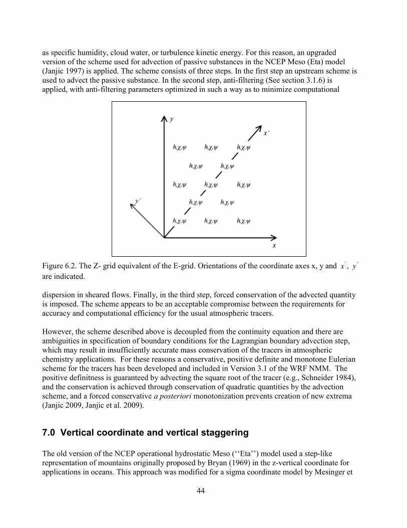
--Rotational momentum as defined on the semi staggered E-grid. The Z-grid equivalent of the E-grid (Janjic 1984) used to define the quantities (6.3.1)–(6.3.4) is shown in Fig. 6.2 together with the orientation of the coordinate axes x, y and x′, y′ appearing in (6.3.1)–(6.3.4). As before, χ and ψ are the velocity potential and the stream function, respectively, and h stands for mass point variables. The symbol ΔA denotes the area of the grid boxes, and the summation sign with the subscripts i, j represents the summation in the horizontal. In case of general flow, the scheme conserves: -- Kinetic energy as defined on the semi-staggered E-grid

( ) ( )2 212 x y y x Vδ ϕ δ ψ δ ϕ δ ψ − + + ∆ ∑ .

-- Momentum as defined on the semi-staggered E-grid.

In (6.3.4), the summation sign indicates the summation over all grid points, and the symbol ΔV denotes the grid box volume in hydrostatic vertical coordinates. The scheme for horizontal advection of temperature also conserves the first and the second moments of temperature. Finally, in the hydrostatic limit, i.e., when dw/dt tends to zero, the exact cancellation is achieved between the contributions of the pressure gradient force to the kinetic energy generation, and the ωα term of the continuity equation, which guarantees consistent transformations between the kinetic and the potential energy, and the conservation of total energy. The relevant finite-difference schemes were presented in Janjic (1977), and their generalizations for the ‘‘isotropic’’, 8-flux divergence operators were discussed in Janjic (1984) and further documented, e.g., in Mesinger et al (1988). The exact energy conservation is not currently required in the case of the fully non-hydrostatic equations. In this case the terms involving ε = (dw/dt)/g are of the order higher than quadratic, and ε=(dw/dt)/g is small compared to unity in weakly non-hydrostatic flows that can be expected in NWP applications. On the other hand, on the scales and in the flow regimes where the contribution of ε=(dw/dt)/g becomes significant, the dissipation starts to play a prominent role creating strong energy sinks. The centered conservative schemes used for advection of the basic dynamic variables develop well known problems in case of advection of positive definite scalars with large spatial variation, such

(6.3.3)

(6.3.4)

44

as specific humidity, cloud water, or turbulence kinetic energy. For this reason, an upgraded version of the scheme used for advection of passive substances in the NCEP Meso (Eta) model (Janjic 1997) is applied. The scheme consists of three steps. In the first step an upstream scheme is used to advect the passive substance. In the second step, anti-filtering (See section 3.1.6) is applied, with anti-filtering parameters optimized in such a way as to minimize computational

Figure 6.2. The Z- grid equivalent of the E-grid. Orientations of the coordinate axes x, y and 'x , 'yare indicated. dispersion in sheared flows. Finally, in the third step, forced conservation of the advected quantity is imposed. The scheme appears to be an acceptable compromise between the requirements for accuracy and computational efficiency for the usual atmospheric tracers. However, the scheme described above is decoupled from the continuity equation and there are ambiguities in specification of boundary conditions for the Lagrangian boundary advection step, which may result in insufficiently accurate mass conservation of the tracers in atmospheric chemistry applications. For these reasons a conservative, positive definite and monotone Eulerian scheme for the tracers has been developed and included in Version 3.1 of the WRF NMM. The positive definitness is guaranteed by advecting the square root of the tracer (e.g., Schneider 1984), and the conservation is achieved through conservation of quadratic quantities by the advection scheme, and a forced conservative a posteriori monotonization prevents creation of new extrema (Janjic 2009, Janjic et al. 2009).

7.0 Vertical coordinate and vertical staggering The old version of the NCEP operational hydrostatic Meso (‘‘Eta’’) model used a step-like representation of mountains originally proposed by Bryan (1969) in the z-vertical coordinate for applications in oceans. This approach was modified for a sigma coordinate model by Mesinger et

45

al. (1988). The advantage of the step-like mountain representation is that the coordinate surfaces are quasi-horizontal. This, however, is not without consequences. For example, internal discontinuities are introduced at the vertical sides of the steps that replace the mountain slopes, and lateral boundary conditions are required at these discontinuities. The formal accuracy of the finite differences at the points next to the internal boundaries is reduced to the first order. In addition to that, if the no slip boundary conditions are used in order to preserve in a simple way the major favorable features of the finite-differencing schemes (cf. Janjic 1977, 1979, 1984), a nonphysical sink of momentum is introduced. Yet another problem is the representation of the physical processes in the surface layer and the planetary boundary layer (PBL). If one wants to represent these processes in a reasonably uniform way throughout the integration domain, including both low-lying and elevated terrain, an approximately equidistant spacing of the vertical levels is required in the lower few kilometers of the atmosphere. However, the vertical resolution needed in order to achieve this goal is still too high. This was indeed one of the major problems in the process of developing the physical package for the Meso (‘‘Eta’’) model (Janjic 1990, 1994). The problem has been greatly alleviated by increasing the vertical resolution over time, which eventually allowed meaningful application of the similarity theory over large parts of the integration domain (Lobocki 1993; Janjic 1996). However, the vertical resolution is still far from satisfactory over elevated areas. This can impair the model’s ability to forecast the diurnal variation of near-surface parameters and local thermally driven circulations in these areas. The hydrostatic Meso model with the step-mountains (‘‘eta coordinate’’) has been producing reasonably good synoptic scale conventional meteorological guidance. Apparently, the blocking by the step-mountains has been able to depict reasonably well the synoptic scale flow around the obstacles. However, with the increasing computing power and model resolutions, as well as the increasing expectations of the users, several problems that could be associated with the step-mountain representation of topography started to surface, particularly at smaller scales, and in mountainous areas. The difficulties appear to be associated with the flow over the obstacles. For example, the model using the step-mountain representation failed to reproduce a catabatic windstorm in the Rockies, while the forecast using the conventional sigma coordinate was quite successful in this respect (Janjic and DiMego 2001). In addition, several recent studies (Adcroft et al. 1997, Gallus 2000, Gallus and Klemp 2000, Janjic and DiMego 2001) indicate that more problems should be expected at higher resolutions. Another problem possibly related to the mountain representation is that the NCEP Meso model using the step-mountains was producing precipitation too far down on the slopes of major orographic obstacles (Staudenmeier and Mittelstadt 1998, Janjic 1998). A similar problem was noticed independently in the operational high resolution runs in the Alpine region made at the Regional Weather Service of Emilia-Romagna, Italy (communicated by Pacagnella). In response to the problem, the Italian meteorologists replaced the step-mountains by the conventional sigma coordinate. In response to the step-mountain problems the hybrid pressure-sigma vertical coordinate option (Arakawa and Lamb 1977) has been introduced into the NMM. With the hybrid coordinate, the coordinate surfaces are flat above and away from the mountains. In the vicinity of the mountains, the hybrid coordinate has increased vertical resolution, and the equations are continuous, without the computational internal boundary conditions that have to be specified with the step-mountains.

46

The sloping coordinate surfaces in the vicinity of the mountains, and the related inaccuracies, are the price to pay for these benefits. Since the hydrostatic pressure is currently used as the vertical coordinate above 400 hPa, the possible inaccuracies due to the sloping coordinate surfaces are restricted only to about the lower half of the mass of the atmosphere. Note that, generally, largest errors in the σ-coordinate occur in the stratosphere. Thus, with the hybrid coordinate, the most serious problems associated with the sloping σ-surfaces are eliminated. In addition, the increased resolution presumably acts in the direction of reducing the computational inaccuracies, and improves the representation of the vertical structure of the PBL over elevated terrain. Figure 7.1 illustrates the distribution of vertical levels in the NNM.

Figure 7.1. The hybrid vertical coordinate used in the NMM. The usual Lorenz staggering of the variables is used in the vertical (Fig. 5.4). The geopotential and the non-hydrostatic pressure are defined at the interfaces of the layers, while all three velocity components and temperature are carried in the middle of the model layers. The vertical velocity is defined at the E-grid mass points.

47

8.0 Boundary Conditions

8.1 Lateral boundary conditions Figure 8.1 illustrates the lateral boundary conditions used in the NMM. The values of velocity and the mass variables are specified only on the outermost rows and columns. On the first row or column in from the outer boundaries, each variable is replaced by a four point average from its surrounding points (Mesinger and Janjic 1974, Mesinger 1977). Inside the domain, the initial values before the averaging are defined by the tendency equations with the advection terms computed using upstream differences on the three rows next to the internal boundary where the four point averaging is applied. In this way, the boundary conditions for advection are well posed.

Figure 8.1. Lateral boundary conditions. H denotes mass variables and V the velocity vector. Enhanced divergence damping (see Section 10.2) is generally applied close to the boundaries. The extent of this damping is user specified.

8.2 Vertical boundary conditions The vertical boundary conditions are:

0σ = and 0p π− = at 0σ = and

0σ = and ( ) 0p πσ

∂ −=

∂ at 1σ = .

Note that the second part of (8.2.1) and (8.2.2) are required for the non-hydrostatic calculations.

(8.2.1)

(8.2.2)

48

9.0 Turbulent mixing and model filters The model has two types of parameterized dissipative processes (that is filters that are not part of the numerical scheme): explicit lateral diffusion (often called horizontal diffusion) and a process called horizontal divergence damping. These components are simply added to the tendencies whose calculations are described earlier.

9.1 Explicit Lateral Diffusion For the horizontal diffusion, the NMM uses a 2nd order, nonlinear Smagorinsky-type parameterization (Janjic 1990). The diffusion has the form:

( )mV K Vt

∂= ∇ ⋅ ∇

∂, ( )h

H K Ht

∂= ∇⋅ ∇

∂.

Here V and H stand for any v point or h point variable, respectively. In the NMM, the exchange coefficient K is flow dependant:

minmK Cd= ∆ , where C is a constant, mind is the minimum grid distance and ∆ is proportional to the horizontal deformation, which in the NMM is modified by the presence of turbulent kinetic energy (Janjic 1990):

( ) ( ) ( ) ( )1/222 2 22 ''2 2 2 2 2

2x y y x x yqu v u v w w C

∆ = ∆ −∆ + ∆ + ∆ + ∆ + ∆ +

.

As before, the operator ∆ followed by a subscript denotes the difference between two neighboring values along the coordinate axis indicated by the subscript. Here 'C is an empirical constant and a constraint is imposed on ∆ such that

maxmin∆≤∆≤∆

where the lower and upper bounds are empirically determined by the need for residual computational damping and the stability criterion, respectively. The default values of the bounds are 0 and infinity, respectively. The q2 (twice the turbulent kinetic energy) term is included to account for the effects of horizontal mixing due to dry convective entrainment and detrainment. The default value of C’ is 50. The relationship between the exchange coefficient for momentum,

mK , and that for heat and moisture, hK is:

h mK K=

(9.1.1)

(9.1.2)

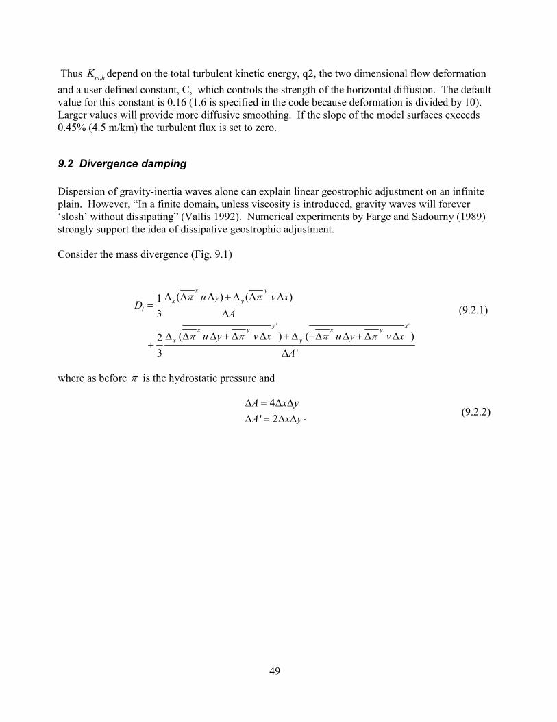
49

Thus ,m hK depend on the total turbulent kinetic energy, q2, the two dimensional flow deformation and a user defined constant, C, which controls the strength of the horizontal diffusion. The default value for this constant is 0.16 (1.6 is specified in the code because deformation is divided by 10). Larger values will provide more diffusive smoothing. If the slope of the model surfaces exceeds 0.45% (4.5 m/km) the turbulent flux is set to zero.

9.2 Divergence damping Dispersion of gravity-inertia waves alone can explain linear geostrophic adjustment on an infinite plain. However, “In a finite domain, unless viscosity is introduced, gravity waves will forever ‘slosh’ without dissipating” (Vallis 1992). Numerical experiments by Farge and Sadourny (1989) strongly support the idea of dissipative geostrophic adjustment. Consider the mass divergence (Fig. 9.1)

' '

' '

( ) ( )13

( ) ( )23 '

x y

x yl

y xx y x y

x y

u y v xD

A

u y v x u y v xA

π π

π π π π

∆ ∆ ∆ + ∆ ∆ ∆=

∆

∆ ∆ ∆ + ∆ ∆ + ∆ −∆ ∆ + ∆ ∆+

∆

where as before π is the hydrostatic pressure and

4

' 2A x yA x y

∆ = ∆ ∆∆ = ∆ ∆ .

(9.2.1)

(9.2.2)

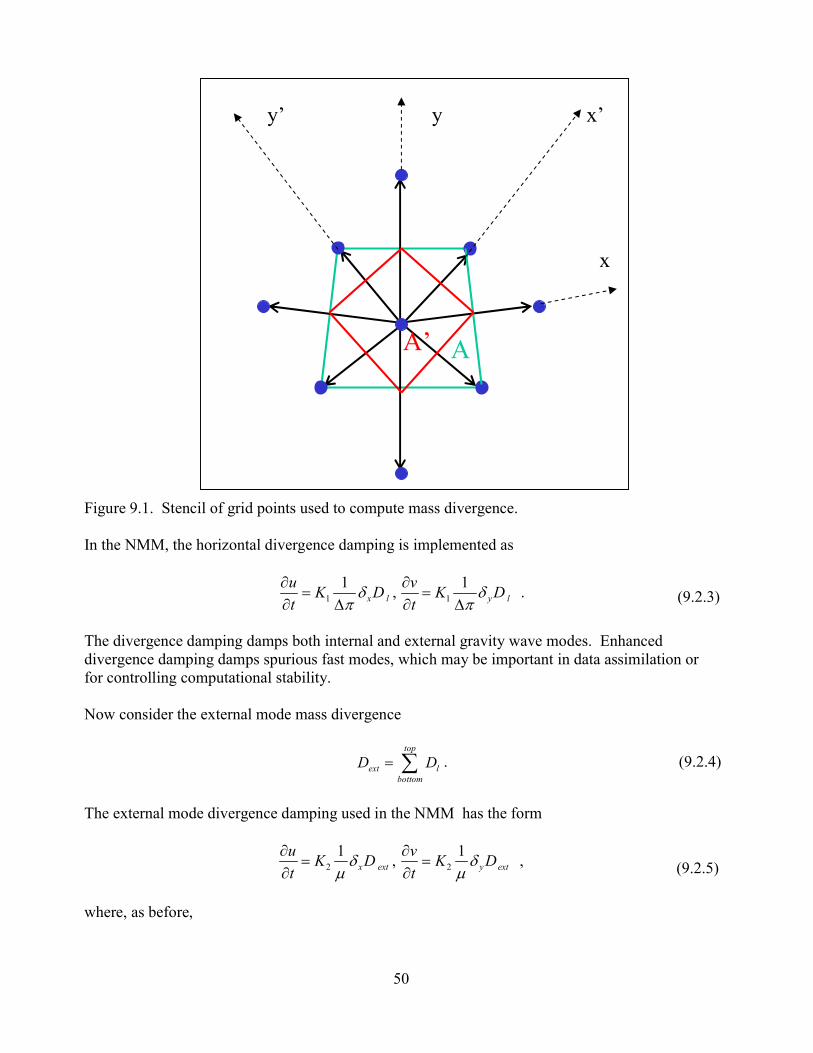
50

Figure 9.1. Stencil of grid points used to compute mass divergence. In the NMM, the horizontal divergence damping is implemented as

1 11 1,x l y l

u vK D K Dt t

δ δπ π

∂ ∂= =

∂ ∆ ∂ ∆ .

The divergence damping damps both internal and external gravity wave modes. Enhanced divergence damping damps spurious fast modes, which may be important in data assimilation or for controlling computational stability. Now consider the external mode mass divergence

top

ext lbottom

D D= ∑ .

The external mode divergence damping used in the NMM has the form

2 21 1, ,x ext y ext

u vK D K Dt t

δ δµ µ

∂ ∂= =

∂ ∂

where, as before,

x’ y’

A A’

x

y

(9.2.3)

(9.2.4)

(9.2.5)

51

bottom topµ π π= − . Integrating formulas (9.2.5) with respect to mass from the bottom to the top of a grid column, one obtains

2

2

1

1

top top

x extbottom bottom

top top

y extbottom bottom

u K Dt

v K Dt

π δ πµ

π δ πµ

∂∆ = ∆

∂

∂∆ = ∆

∂

∑ ∑

∑ ∑

and finally,

2

2 .

top

x extbottom

top

y extbottom

u K Dt

v K Dt

π δ

π δ

∂∆ =

∂

∂∆ =

∂

∑

∑

Thus, only the external mode is affected. The combination of the horizontal and external mode divergence damping also can be used in the NMM and has the form

1 2

1 2

1 1

1 1 .

x l x ext

y l y ext

u K D K Dt

v K D K Dt

δ δπ µ

δ δπ µ

∂= +

∂ ∆

∂= +

∂ ∆

The divergence damping is applied in additive split mode after adding the contributions on the right hand sides of (3.2.21) and (3.2.22). In the code, the constant controlling the strength of the damping is CODD. The default value is 6.4, which corresponds to weak divergence damping.

,

(9.2.6)

(9.2.8)

(9.2.9)

(9.2.7)

52

10.0 References Adcroft, A., C. Hill and J. Marshall 1997: Representation of topography by shaved cells in a

height coordinate ocean model. Mon. Wea. Rev, 125, 2293–2315.

Ames, W. F., 1969: Numerical methods for partial differential equations. London: Nelson, 291 pp.

Arakawa, A. and Lamb, V.R. 1977: Computational design of the basic dynamical processes of the UCLA general circulation model. Meth. Comp. Phys., 17, 173–265.

Bryan, K., 1969: A numerical method for the study of the circulation of the World Ocean. J Comp Phys., 135(2), 347–376.

Farge, M. and R. Sadourny, 1989: Wave-vortex dynamics in rotating shallow water. J. Fluid Mech., 206, 433-462.

Gadd A. J., 1974: An economical explicit integration scheme. Meteorological Office Tech. Note, 44, 7 pp. [London Road, Bracknell, Berks. RG12 2SZ, U.K.]

Gallus, W.A. Jr., 2000: The impact of step orography on flow in the Eta model: Two contrasting examples. Wea. and Forecasting, 15, 630–639.

Gallus, W. A. Jr. and J. B. Klemp 2000: Behavior of flow over step orography. Mon. Wea. Rev., 128, 1153–1164.

Gavrilov, M. B. and Z. I. Janjic, 1989: Computed rotational energy spectra of two energy and enstrophy conserving schemes on semi-staggered grids. Meteo. and Atmos. Phys., 41, 1-4.

Janjic, Z., 2009: Further development of a model for a broad range of spatial and temporal scales. Preprints, 23d Conference on Weather Analysis and Forecasting/19th Conference on Numerical Weather Prediction, American Meteorological Society, May 31-June 5 2009, Omaha, Nebraska.

Janjic, Z., H. Huang and S. Lu, 2009: A unified atmospheric model suitable for studying transport of mineral aerosols from meso to global scales. IOP/Electronic Journals, Conf.Series: Earth and Environmental Science (collection of papers from WMO/GEO Expert Meeting on an International Sand and Dust Storm Warning System Meeting, 7-9 November, Barcelona, Spain), Vol. 9, 6pp. http://www.iop.org/EJ/toc/1755-1315/7/1

Janjic, Z. I., 2003: A Nonhydrostatic Model Based on a New Approach. Meteo. and Atmos. Phys., 82, 271-285. http://dx.doi.org/10.1007/s00703-001-0587-6

Janjic, Z. I., 2001: Nonsingular Implementation of the Mellor-Yamada Level 2.5 Scheme in the NCEP Meso model. National Centers for Environmental Prediction Office. Note #437.

Janjic, Z. I., 1998: Capabilities of limited area numerical models in predicting heavy precipitation events and possibilities for further improvement. In: Meeting of the World Federation of Scientists, Working Group on Defense Against Floods and Unexpected Meteorological Events, Geneva, 19-20 Nov. (invited introductory lecture).

53

Janjic, Z. I., 1997: Advection scheme for passive substances in the NCEP Eta model. Research Activities in Atmospheric and Oceanic Modeling, WMO, Geneva, CAS/JSC WGNE, 3.14.

Janjic, Z. I., 1996: The surface layer parameterization in the NCEP Eta Model. Research Activities in Atmospheric and Oceanic Modeling, WMO, Geneva, CAS/JSC WGNE, 4.16-4.17.

Janjic, Z. I., 1994: The step-mountain eta coordinate model: further developments of the convection, viscous sub layer and turbulence closure schemes. Mon. Wea. Rev., 122, 927-945.

Janjic, Z. I., 1990: The step-mountain co-ordinate: physical package. Mon. Wea. Rev., 118, 1429-1443.

Janjic, Z. I., 1984: Non-linear advection schemes and energy cascade on semi-staggered grids. Mon. Wea. Rev., 112, 1234-1245.

Janjic, Z. I., 1979: Forward-backward scheme modified to prevent two-grid-interval noise and its application in sigma coordinate models. Contributions to Atmos. Phys., 52, 69-84.

Janjic, Z. I., 1977: Pressure gradient force and advection scheme used for forecasting with steep and small scale topography. Contributions to Atmos. Phys., 50, 186-199.

Janjic, Z. I., 1977: Contributions to the enhancement of accuracy of vertical differencing in numerical models of the atmosphere in the areas with steep orography. Limited Area Forecasting Model with Primitive Equations, Research Project ``Weather Forecasting in Yugoslavia'', Volume No. 4, FHMI, Belgrade, 1978, 112 pp., in Serbian Federal Hydro meteorological Institute, P.O.B. 604, YU-11001 Belgrade, Yugoslavia.

Janjic, Z. I., T. L. Black and G. DiMego, 1998: Recent NCEP contributions toward development of a mesoscale model. Research Activities in Atmospheric and Oceanic Modeling. WMO, Geneva, CAS/JSC WGNE.

Janjic, Z. I., and G. DiMego, 2001: Effects of mountain representation and non-hydrostatic dynamics in a case of orographic precipitation. Preprints, Symposium on Precipitation Extremes: Prediction, Impacts and Responses. 81st Annual Meeting of the Amer. Meteor. Soc., Albuquerque, NM, 14-18 January 14-18. Amer. Meteor. Soc., Boston, 24-28.

Janjic, Z. I., J. P. Gerrity, Jr. and S. Nickovic, 2001: An alternative Approach to Non-hydrostatic Modeling. Mon. Wea. Rev., 129, 1164-1178.

Janjic, Z. I. and F. Mesinger, 1989: Response to small-scale forcing on two staggered grids used in finite-difference models of the atmosphere. Quart. J. Royal Meteor. Soc., 115, 1167-1176.

Janjic, Z. I. and F. Mesinger, 1984: Finite-difference methods for the shallow water equations on various horizontal grids. Numerical Methods for Weather Prediction, Vol. 1, Seminar, ECMWF, 1983, Reading, U.K., 29-101, Shinfield Park, Reading, Berkshire RG2 9AX, U.K.

Janjic, Z. I. and A. Wiin-Nielsen, 1977: On geostrophic adjustment and numerical procedures in a rotating fluid. J. Atmos. Sci., 34, 297-310.

54

Laprise, R., 1992: The Euler equation of motion with hydrostatic pressure as independent coordinate. Mon. Wea. Rev., 120 (1), 197-207.

Lobocki L 1993: A procedure for the derivation of surface layer bulk relationships from simplified second-order closure models. J Appl Meteor., 32: 126–138.

Mesinger, F., 1977: Forward-backward scheme, and its use in a limited area model. Contrib. Atmos. Phys., 50, 200-210.

Mesinger, F. and Z. I. Janjic, 1974: Noise due to time-dependent boundary conditions in limited area models. Research Activities in Atmospheric and Oceanic Modelling, The GARP Programme on Numerical Experimentation, Rept. No. 4, 31-32.

Mesinger, F., Z. I. Janjic, S. Nickovic, D. Gavrilov and D. G. Deaven, 1988: The step-mountain coordinate: model description and performance for cases of Alpine lee cyclogenesis and for a case of an Appalachian redevelopment. Mon. Wea. Rev., 116, 1493-1518.

Randall, D. A., 1994: Geostrophic adjustment and the finite difference shallow-water equations. Mon. Wea. Rev., 122, 1371–1380.

Schneider, H. R., 1984: A Numerical Transport Scheme which Avoids Negative Mixing Ratios. Mon. Wea. Rev., 112, 1206–1217.

Staudenmeier, M. J. and J. Mittelstadt, 1998: Results of the western region evaluation of the Eta-10 model. Preprints,12th Conf. on Numerical Weather Prediction, Phoenix, AZ, 11–16 January. Amer. Meteor. Soc., Boston, 131–134.

Vallis, G., 1992: Mechanisms and parameterizations of geostrophic adjustment and a variational approach to balanced Ffow. J. Atmos. Sci., 49(13), 1144–1160.

Winninghoff, F. J., 1968: On the adjustment toward a geostrophic balance in a simple primitive equation model with application to the problems of initialization and objective analysis. Ph.D. Thesis, Dept. Meteor. Univ. California, Los Angeles, CA