Near-bottom seismic profiling: High lateral variability

University of New Hampshire University of New Hampshire

University of New Hampshire Scholars' Repository University of New Hampshire Scholars' Repository

Affiliate Scholarship Center for Coastal and Ocean Mapping

11-1980

Near-bottom seismic profiling: High lateral variability, anomalous Near-bottom seismic profiling: High lateral variability, anomalous

amplitudes, and estimates of attenuation amplitudes, and estimates of attenuation

R. C. Tyce University of California - San Diego

Larry A. Mayer University of New Hampshire, [email protected]

F. N. Spiess University of California - San Diego

Follow this and additional works at: https://scholars.unh.edu/ccom_affil

Part of the Geophysics and Seismology Commons, and the Oceanography and Atmospheric Sciences

and Meteorology Commons

Recommended Citation Recommended Citation Tyce, R. C., Mayer, L.A., and Spiess, F. N., 1980. Near-bottom seismic profiling: High lateral variability, anomalous amplitudes, and estimates of attenuation, Jour. Acoustical Society of America, vol. 68, no. 5, pp. 1391-1402. http://dx.doi.org/10.1121/1.385106

This Article is brought to you for free and open access by the Center for Coastal and Ocean Mapping at University of New Hampshire Scholars' Repository. It has been accepted for inclusion in Affiliate Scholarship by an authorized administrator of University of New Hampshire Scholars' Repository. For more information, please contact [email protected].

https://scholars.unh.edu/

https://scholars.unh.edu/ccom_affil

https://scholars.unh.edu/ccom_home

https://scholars.unh.edu/ccom_affil?utm_source=scholars.unh.edu%2Fccom_affil%2F69&utm_medium=PDF&utm_campaign=PDFCoverPages

http://network.bepress.com/hgg/discipline/158?utm_source=scholars.unh.edu%2Fccom_affil%2F69&utm_medium=PDF&utm_campaign=PDFCoverPages



mailto:[email protected]

Near-bottom seismic profiling: High lateral variability, anomalous amplitudes, and estimates of attenuation

R. C. Tyce, L. A. Mayer, a) and F. N. Spiess University of California, San Diego, Marine Physical Laboratory, Scripps Institution of Oceanography, San Deigo, California 92152 (Received 13 February 1980; accepted for publication 13 August 1980)

For almost a decade !the Marine Physical Laboratory of Scripps Institution of Oceanography has been conducting near-bottom geophysical surveys involving quantitative seismic profiling. Operating initially at 4 kHz and more recently at 6 kHz, this system has provided a wealth of fine scale quantitative data on the acoustic properties of ocean sediments. Over lateral distances of a few meters, 7-dB changes in overall reflected energy as well as 10-dB changes from individual reflectors have been observed. Anomalously high amplitudes from deep reflectors have been commonly observed, suggesting that multilayer interference is prevalent in records from such pulsed ½w profilers. This conclusion is supported by results from sediment core physical property work and related convolution modeling, as well as by the significant differences observed between 4- and 6-kHz profiles. In general, however, lateral consistency has been adequate in most areas surveyed to permit good estimates of acoustic attenuation from returns from dipping reflectors and sediment wedges.

PACS numbers: 43.30.Bp, 43.30.Dr, 92.10.Vz, 43.40.Ph _

INTRODUCTION

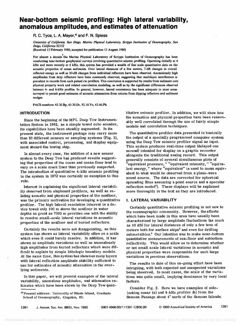
Since the beginning of the MPL Deep Tow Instrumen- tation System in 1962. as a simple towed echo sounder, its capabilities have been steadily augmented. In its present state, the instrument package may carry more than 20 different sensors or sampling systems (Fig. 1), with associated control, processing, and display equipment aboard the towing ship.

In almost every case, the addition of a new sensor system to the Deep Tow has produced results suggesting that properties of the ocean and ocean floor tend to vary on a scale much finer than previously suspected. The introduction of quantitative 4-kHz seismic profiling to the system in 1972 was certainly no exception to this rule.

Interest in explaining the significant lateral variability observed from shipboard profilers, as wel• as re- lating acoustic and physical properties of the seafloor, was the primary motivation for developing a quantitative profiler. The high lateral resolution inherent in a de- vice towed only 100 m above the seafloor in water depths as great as 7000 m provides one with the ability to resolve small-scale lateral variations in acoustic

properties of the seafloor and of buried reflectors.

Certainly the results were not disappointing, as this system has shown us lateral variability often on a scale which even it could barely resolve. In addition, it has shown us amplitude variations as well as anomalously high amplitudes from buried reflectors which were dif- ficult to explain by simple lithologic boundary models. At the same time, this system has shown us many layers with lateral reflection amplitude stability stffficient to use for estimates of acoustic attenuation in the over-

lying sediments.

In this paper, we will present examples of the lateral variability, anomalous amplitudes, and attenuation estimates which have been shown by the Deep Tow quan-

a•Present address' University of Rhode Island, Graduate School of Oceanography, Kingston, RI.

titative seismic profiler. In addition, we will show how the acoustics and physical properties have been reasonably well correlated through the use of fairly simple models and convolution techniques.

The quantitative profiler data presented is basically the output of a specially programmed computer system using the Deep Tow seismic profiler signal as input. This system produces real-time output (delayed one second) intended for display on a graphic recorder alongside the traditional analog record. This output generally consists of several simultaneous plots of "equivalent pressure, "equivalent intensity," equivalent energy," where "equivalent" is used to mean equivalent to what would be observed from a plane-wave sound source. The data are corrected for spherical spreading (thus assuming a point source and a specular reflection model•'). These displays will be explained more thoroughly in the text as they are introduced.

I. LATERAL VARIABILITY

Certainly quantitative seismic profiling is not new to the oceanographic community. However, the efforts which have been made in this area have usually been characterized by large amplitude fluctuations (as much as 10 dB) for lateral distances of only a few tens of meters both for surface ships 3 and even for drifting submersibles. 4 Our intention was to make near-bottom

quantitative measurements of sea-floor and subbottom reflectivity. This would allow us to determine whether or not small scale lateral variations in acoustic and

physical properties were responsible for such large variations in previous observations.

The results to date of this on-going effort have been intriguing, with both expected and unexpected variations being observed. In most cases, the scale of the variations was quite small, implying dominance by very local factors.

Consider Fig. 2. Here we have examples of side- looking sonar (a) and 4-kHz profiler (b) from the Samoan Passage about 4 ø north of the Samoan Islands.

1391 J. Acoust. Soc. Am. 68(5), Nov. 1980 0001-4966/80/111391-12500.80 ¸ 1980 Acoustical Society of America 1391

Redistribution subject to ASA license or copyright; see http://acousticalsociety.org/content/terms. Download to IP: 132.177.229.80 On: Wed, 07 Oct 2015 13:49:32

EMERGENCY '• -• ¾œL•i'•ETER) TR;"NS:'•'c•NoER HYDROPHONE '• X :"i•[' /

'' : TV • U•AR'D-:LO'OKING [• •.' / • SONAR ' / (SUSPENDED

TRANSPONDER • ' : ........ t'::::'•:•:•' .... / I • •HOTO • / PARTICLE FtLTER)

• *•: •?•:" ';:• ..... ' ....................... •"••••••:..- ••••'• ' ':•;•{'"•?.'• ." :'•:•/'•:':: ..... '•-'?:::':" '•'"'""•';•••':•::'::.':•:':"•. ...... ::•"•"•::•?'"{?': / OBSTACLE • -• •;.. ;•:"•'""•'•':•'::.::::•'•:•::;•.':•:;•.".': :: .. •:...;•?•:;•:.•-•;'-•J•'•'w' :• •:..?:'•'"' ...... '•'•;•"•'i• ?-:{?':'""•'-' • AVOIOANCE SONAR :•:•.•. • .• .... , . ., . ß • • •-. 1.:-,.:•::.::•;..• • •- , ß • .... .•..-.•r• :.....•...• ..... •r ..... .• :--.'..-:'•:".-:..:-: •:'...• . •-.• ':•/-: . ß .

..• •:. .•/•.-:, .:::. ?•:•:.. ....... '•..•.•••.••• '• ....... - .... . •:.:-..; ..... '. • . •f :•-? •::.•..:....:•.•.• .• ..• •:; " ':'•q •:; ' "'?:: ...... ::":" "• :: "" '""•:•" ............... ' ........ ":::::'"'"'::'""•' • .... • •:: ' •' ::"•:.'"'•'

4 kHz T:RA;NSD-UCER ' ;r :.•'7%•' '" ' .......... ' ........... ' ...... :" •"'• '..' ... •"•?•*"'•• - .... :::... '• . :. • •.. • ..... .:..-.• ' • / :• ...................... ::•.:: ......... ..:..::•;:• ....................... •:: ......................... :• ...... ,•..L-•:.:Lj_•••""

• " •" • LOOKING SONAR , • / • .... ' ' ' '" : '•' •R'E ......... ..... ' ..... '•'•"- •;'•i •J' •

•Sr•:A'•'O'•'A)' :?½ .../..-• ' ... .•••" . '••-:::•' :•.•':•:&:•;] .•:NETOM:ETER • L ............ '••••••••-: .......... • • S•:M'•:U#•'

KEY

TOWING CABLE =' STANDARD EQUt:PMENT

[NEPHE•OMETœR) =. OPTIONAL EQUIPMENT

FIG. 1. Schematic of deep tow instrumentation system.

'• ' .... •'x ' ß ................... :.it'.;...:::'....-"::-'--" '" • '"' ' i ..... .'. ......... .;:i"::::,?,:::•i',i',:':i•11i:::,;,:..: '-" ".:::.:.:.-.---.,.,'::::,--::::'i.,:...:::::.:.:i.,:-*.:; .:.--...•:-. '...• •;. ' •:'•'::•/• .- ..' .- ..,• . . ...• ..... '•' ..... ...: .::.?. :::.::.... ':•....: :::::::?:::::::::: :::::•. .•::: :•...:.:::.:.:.:•...: :•::•::{..: .• :: .fWA'TER SAMPLERS) r, r," /

-.... .• ..... ß •, ..- • • •' ,•,•::•':-•.::.?•?:'....:..; ....... .

....... ...... .....

The side-looking sonar records shows little of note (or_her than the beam pattern stripes), suggesting that the bottom is relatively smooth. The profiler record shows a well lineated pond of sediments over a rough

(b)

...:.,...•.._•.-.,•/:.•:":T'. ...................... ::i• • ...... !' ......... ....... •........•... ....... •.:.. ; ....... -.•,;. ....... • •;.-----,• .... . ........ .•••.•.

......................... .: :.-•.•;:-:-.::;ii-/:•i-:-..i;:;.;..,il ---•----- -•-..-.-• ..., ..•/......•••:;•i:•::•:•qiii:;•.;•:•:•;:•.;.i•"4`?.::..:i4•.•.•;•!<:•.•;/•i•;::•.i•i•i•; • ::•::,?:--:'•'-•:::!i'.'.?;:•-;•?:,:•.½•:'i:•-?•:.:i,?-'• i ...... •:• .!-'..•.'-• ':'•-•:.- .•--•. :•-'•::-•.:'•:---.••-•i•.•-,;i•!!--..;.. ::.:i•-•--:% :•-:-:•:•i•- =============================/-::--..•:,:•.•i,:.:,.:,:•;::•,..-:-.:::.i.., ':•':- ::-:-:. -:'•::•": ........... '" ' ...... ' ......... ::'"- -' -"•:'""':'•'-": ::' "" '"" :':'•";'•'::'• ' '?'•' i':•::'; ':' ":•:-: !'--•'•:•":'- ....... ' -.-.'"'"?•'::-:':" •':::': •- •";/"':' '" '•' ':' '•"• ........ :'•:"•" '::':•-'?:•?-•:'•;:.;•'::'?•;i:•: •-' ß :.:..:.--.-..,..• .............. -•:?.•,:•...-:..•.-':::.:•.•.•. •,•:.•. • - ....... . .... :!•!•:-.•.-.';•:.-,..•.•;.:.•:. •.• ...... • .-•:---•:-• ...•... ::.:.•:.•..- ..... ...:;•:..:•.:::.•:..:•.•:•....•..,,...;•:.•..:.:..,.....:•:•.......

...... ' ........ t --'i I I

?5ore

•TG. 9.. :Near-bottom ski. e-looking so•ar (a) and •-•:[-]:•. seismic profiler (b) records from an area of the Samoan Passage North of Somoa.

acoustic basement. Some variability in reflectivity is suggested in this record, but the limited dynamic range of the recorder (about 10 dB) tends to obscure such variations. This is generally the case for most variable density recorders.

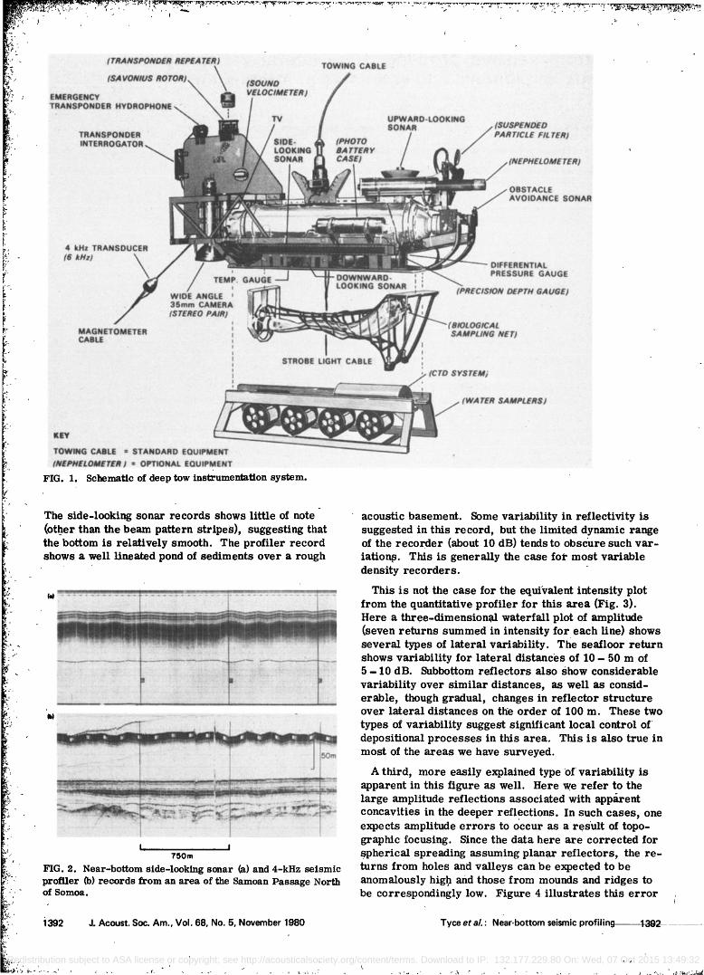
This is not the case for the equivalent intensity plot from the quantitative profiler for this area (Fig. 3). Here a three-dimensional waterfall plot of amplitude (seven returns summed in intensity for each line) shows several types of lateral variability. The seafloor return shows variability for lateral distances of 10- 50 m of 5- 10 dB. Subbottom reflectors also show considerable

variability over similar distances, as well as considerable, though gradual, changes in reflector structure over lateral distances on the order of 100 rn. These two

types of variability suggest significant local control of depositional processes in this area. This is also true in most of the areas we have surveyed.

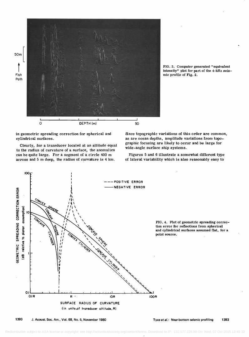
A third, more easily explained type of variability is apparent in this figure as well. Here we refer to the large amplitude reflections associated with apparent concavities in the deeper reflections. In such cases, one expects amplitude errors to occur as a result of topographic focusing. Since the data here are corrected for spherical spreading assuming planar reflectors, the returns from holes and valleys can be expected to be anornalously high and those from mounds and ridges to be correspondingly low. Figure 4 illustrates this error

1392 J. Acoust. Soc. Am., Vol. 68, No. 5, November 1980 Tyce etaL' Near-bottom seismic profiling- 1392


5Om

t Fish

Path

FIG. 3. Compute• generated "equivalent intensity" plot for part of the 4-kHz seismic profile of Fig. 2.

i I I

O DEPTH (m)

in geometric spreading correction for spherical and cylindrical surfaces.

Clearly, for a transducer located at an altitude equal to the radius of curvature of a surface, the anomalies can be quite large. For a segment of a circle 400 m across and 5 m deep, the radius of curvature is 4 km.

Since topographic variations of this order are common, as are ocean depths, amplitude variations from topographic focusing are likely to occur and be large for wide.angle surface ship systems.

Figures 5 and 6 illustrate a somewhat different type of lateral variability which is also reasonably easy to

100

o

o

n. •. 10

i.u I

O.I

OIR

i I i I ii

Ii II

i

I

i

I i

I

I

I1•

II1\ I1•\

I

\

\

POSITIVE ERROR

• NEGATIVE ERROR

R - IOR

SURFACE RADIUS OF CURVATURE

(in units•f transducer altitude,R)

IOOR

FIG. 4. Plot of geometric spreading correction error for reflections from spherical and cylindrical surfaces assumed fiat, for a point source.

1393 J. Acoust. Soc. Am., Vol. 68, No. 5, November 1980 Tyce et al ß Near-bottom seismic profiling 1393


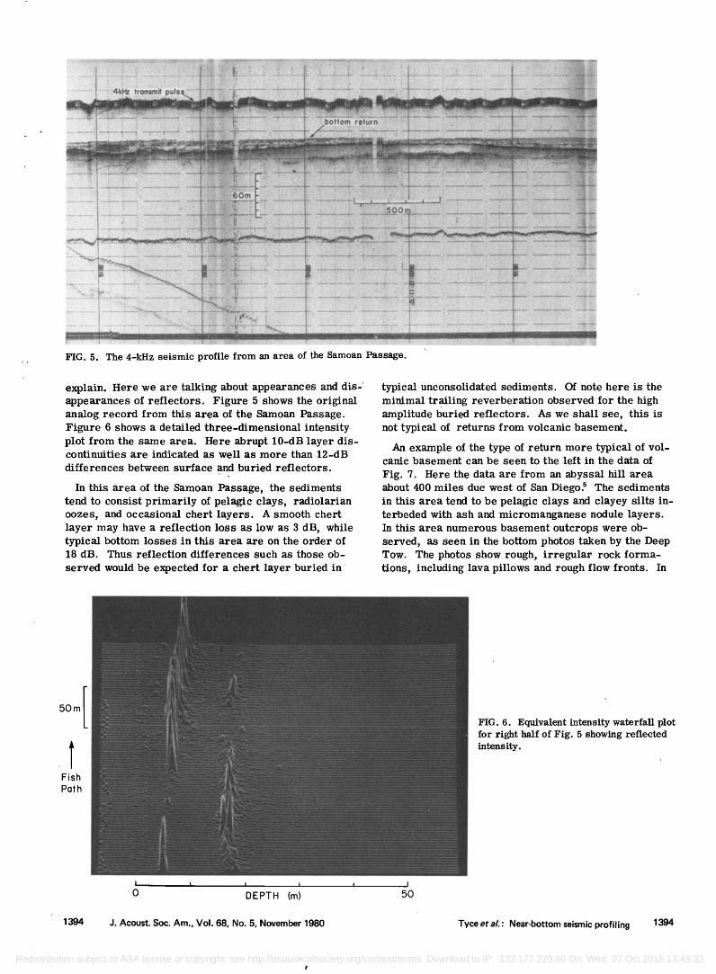
FIG. 5. The 4-kHz seismic profile from an area of the Samoan Passage.

explain. Here we are talking about appearances and dis- appearances of reflectors. Figure 5 shows the original analog record from this area of the Samoan Passage. Figure 6 shows a detailed three-dimensional intensity plot from the same area. Here abrupt 10-dB layer dis- continuities are indi,cated as well as more than 12-dB

differences between surface and buried reflectors.

In this area of the Samoan Passage, the sediments tend to consist primarily of pelagic clays, radiolarian oozes, and occasional chert layers. A smooth chert layer may have a reflection loss as low as 3 dB, while typical bottom losses in this area are on the order of 18 dB. Thus reflection differences such as those ob-

served would be expected for a chert layer buried in

typical unconsolidated sediments. Of note here is the minimal trailing reverberation observed for the high amplitude buried reflectors. As we shall see, this is not typical of returns from volcanic basement.

An example of the type of return more typical of volcanic basement can be seen to the left in the data of

Fig. 7. Here the data are from an abyssal hill area about 400 miles due west of San Diego? The sediments in this area tend to be pelagic clays and clayey silts in- terbeded with ash and micromanganese nodule layers. In this area numerous basement outcrops were observed, as seen in the bottom photos taken by the Deep Tow. The photos show rough, irregular rock forma- tions, including lava pillows and rough flow fronts. In

50m

Fish

Path

FIG. 6. Equivalent intensity waterfall plot for right half of Fig. 5 showing reflected intensity.

I I I I

DEPTH (m)

1394 J. Acoust. Soc. Am., Vol. 68, No. 5, November 1980 Tyce et aL' Near-bottom seismic profiling 1394


ß ' .... :" ..... '•': ............... :. •'"•::::.:::: !'" , [ Transmit Pulse

"' ................................ "!" .. ...... ........ :-' .......... ' . I00 m• • ' ....... :"" :71:':' .................. ..'•i..?.• 4 kHz bott'om profile

500 m

:.:::•: .-• .,:: ,:•. ?' •; :";;•',' , :• •;:•' • .... •.•"•.•¾.." •.'-•.-• .-•..:.-•:- ::•,,.'.,•.•..::. ..... .•.•::.• •.:,. ,.•-•:--'---•:j• :• ½:' .. •.,:• .:::• ......... ":•:-'-•';•'; '--•: .... '•;•%•:'• -•?:- -:•-• :•"•-:-•'•.---•.•:•"•:': , ,-- ?•"'" • .... •:• '-'-':• 'o,•'• " :?• :-•.•'...•:::-'-•'-•?:? .... . ................ .•.•::'.•;:•::•:-•.•':•'"'- ,,•...•...•:.•.•.-.- -:...•;:-;;• :•.•-•:•,. .••,. .••.••..•:.' •: .•:• ..... ..•:..... ..... •::. "'•:;.:-::'•:• :•:'•:. ............... ::;•,:::.•L-•:.:.•.'•---•7;•',.•" '""•"•.-_:•-'•'--• ' -;•: '•' --:'• ':•.' ..•'-." ". •. ".'••,:•:• ....... :•'-.'•'•.. -•: '••••:•.•:::...::.::- . .:..•;•'•.::...::.: ...... ..... •, .• ........ • • .......... '.,.:,.',.: ................ .,...,.:.'..;.::.';;: ""--•-:.-:;..-.:;.::;--;.;.:.'.-..-: ..... -:--•-.--t -'•- -••:-: .::. •;... -: .................................... • ................................ ,• .:• •,.• •:•:-•::.•':-.-•-•:Z•:• •

•-•:•%•-.•-• • •,•.½-.•-• •.-•;•;•-•.,•:•?• •:•:•;•:.•?: •:•,-•,:•:•.•:•::'•;•:-•:•:::.•::::•,r•..-•::•:::•:• •:.-•::. .......... :: •:.• .............................. ,, ..:•'•-•:...•........•....? ........................... •::•.: ..................... . .............. . ................. . ................. . ......................... ...:.•;'•.•.,•..:.:..•;,:+ :-.:.:.,•.:.,- ......... . ............ . .......................... ::•;•:•:+,.:.•:::.';;;:.:•.:;; .................... ..... . '• .;.:•.• . •.-,',•-.•. ,.-,'..-,..:..,.,. .......... ....½:.-....+.-.-.,• -.• •,,.. ......... .,.•:. ,• .......... /, •-..-::,•,....• .... ..•..,- ......... ;..,,..:...• ....................

'•':"• ...... ' - ..•. ß ;...•..t .... ,,..::;;:.; ..... ...:•..•..• ••... -. .... -•..•.•..•.. '""• .... :... •.......:; ..... ;.•. .;/ ' ::.: ?.:•:.•:.,•:•:,: •.-.

•:•. •: ,., ,:.--....: .•::. •. ,.. •, • .:.•,..•::.:. ........... -•:.:• .....•.. •......• ...,: •...•.........,:.. ........ , . • ...•/--,., ..; •. ,.. ::.- ...... .,, ,:....• :•: ..... ; ,; •,.•--•:•.•.•?--'•;?•.'-•-.•.•.•'•:: .. -:::: - .... ., -. ... ......... . . , .......... "•'•'.•"•'t:--•: '•½.. '-•:•';.'•- :.::-•;•;'--,:•:;,.::.' :-: '. -, ....•.. - ...... - -. ..... - ...... ':-' ....

........... •: ,.•.: :. : •:...•;.::..:..::.• .•-•,., • . . ....... : ,...... ...... . ...... -....:..:•:

..... . --• • .•:...... ...... -• .... •.•?:..•: •:,. •'•'-'•.•-:,•;'•..:..-'-' ,:..•:...•-•.• ......... .;:.;• •::• .... •::....•:.::. . , , • .::: •q•i•, •r•ss•r•-..:•; •.. •...,•.. .... •:.- --•-,.: • ,:: .• ...... ,:-:,.• ........ •

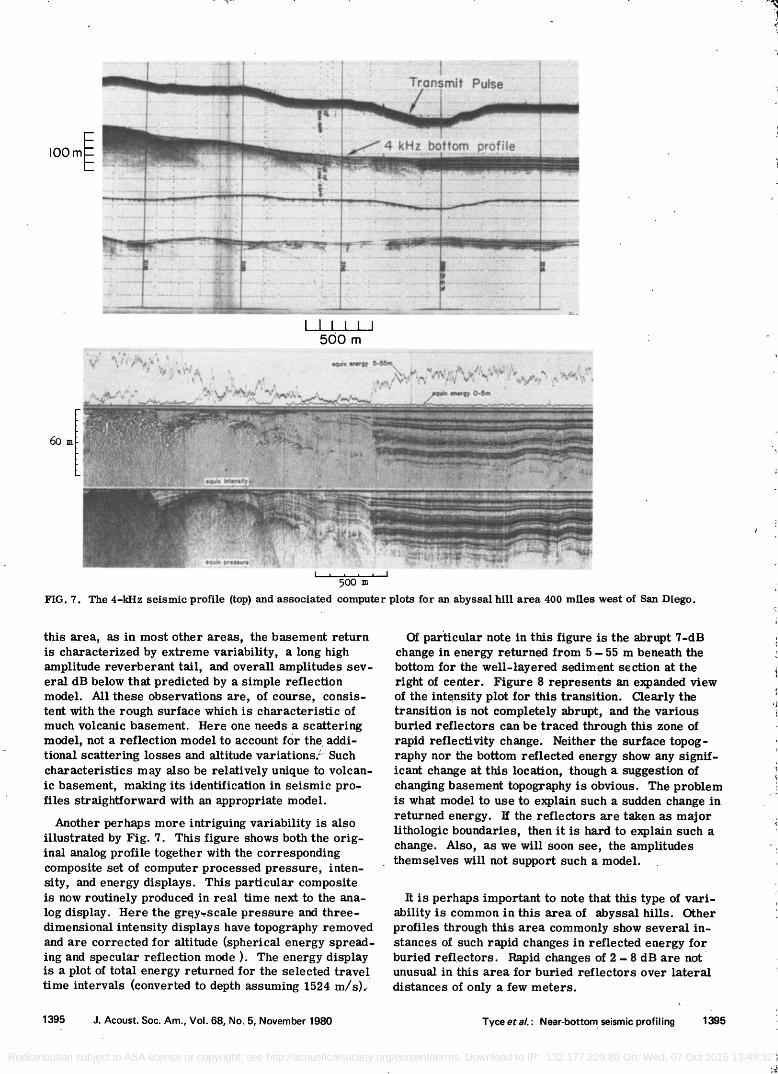
• •00 • FIG. 7. The 4-kHz seismic profile (top) and associated computer plots for an abyssal hill area 400 miles west of San Diego.

this area, as in most other areas, the basement return is characterized by extreme variability, a long high amplitude reverberant tail, and overall amplitudes several dB below that predicted by a simple reflection model. All these observations are, of course, consistent with the rough surface which is characteristic of much volcanic basement. Here one needs a scattering model, not a reflection model to account fc;r the additional scattering losses and altitude variations. Such characteristics may also be relatively unique to volcanic basement, making its identification in seismic profiles straightforward with an appropriate model.

Another perhaps more intriguing variability is also illustrated by Fig. 7. This figure shows both the original analog profile together with the corresponding composite set of computer processed pressure, intensity, and energy displays. This particular composite is now routinely produced in real time next to the analog display Here the grqy-scale pressure and three- dimensional intensity displays have topography removed and are corrected for altitude (spherical energy spreading and specular reflection mode ). The energy display is a plot of total energy returned for the selected travel time intervals (converted to depth assuming 1524 m/s).

Of particular note in this figure is the abrupt 7-dB change in energy returned from 5- 55 m beneath the bottom for the well-layered sediment section at the right of center. Figure 8 represents an expanded view of the intensity plot for this transition. Clearly the transition is not completely abrupt, and the various buried reflectors can be traced through this zone of rapid reflectivity change. Neither the surface topography nor the bottom reflected energy show any significant change at this location, though a suggestion of changing basement topography is obvious. The problem is what model to use to explain such a sudden change in returned energy. If the reflectors are taken as major lithologic boundaries, then it is hard to explain such a change. Also, as we will soon see, the amplitudes themselves will not support such a model.

It is perhaps important to note that this type of variability is common in this area of abyssal hills. Other profiles through this area commonly show several in- stances of such rapid changes in reflected energy for buried reflectors. Rapid changes of 2- 8 dB are not unusual in this area for buried reflectors over lateral

distances of only a few meters.

1395 J. Acoust. Soc. Am., Vol. 68, No. 5, November 1980 Tyce etaL: Near-bottom seismic profiling 1395


5Om

Fish

Path

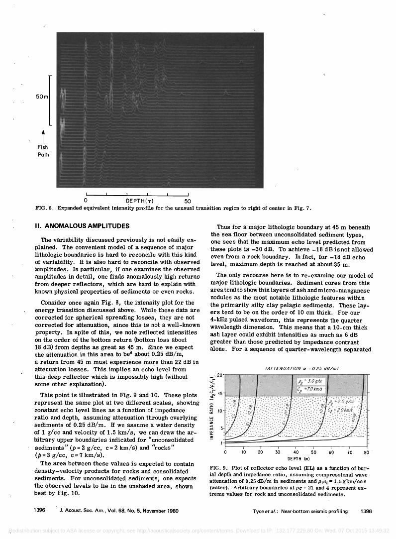
O DEPTH(m) 50 FIG. 8. Expanded equivalent intensity profile for the unusual tran}ition region to right of center in Fig. 7.

II. ANOMALOUS AMPLITUDES

The variability discussed previously is not easily explained. The convenient model of a sequence of major lithologic boundaries is hard to reconcile with this kind of variability. It is also hard to reconcile with observed amplitudes. In particular, if one examines the observed amplitudes in detail, one finds anomalously high returns from deeper reflectors, which are hard to explain with known physical properties of sediments or even rocks.

Consider once again Fig. 8, the intensity plot for the energy transition discussed above. While these data are corrected for spherical spreading losses, they are not corrected for attenuation, since this is not a well-known property. In spite of this, we note reflected intensities on the order of the bottom return (bottom loss about 18 dB) from depths as great as 45 m. Since we expect the attenuation in this area to be 6 about 0.25 dB/m, a return from 45 m must experience more than 22 dB in attenuation losses. This implies an echo level from this deep reflector which is impossibly high (without some other explanation).

This point is illustrated in Fig. 9 and 10. These plots represent the same plot at two different scales, showing constant echo level lines as a function of impedance ratio and depth, assuming attenuation through overlying sediments of 0.25 dB/m. If we assume a water density of l g/cc and velocity of 1.5 kin/s, we can draw the arbitrary upper boundaries indicated for "unconsolidated sediments" (p = 2 g/cc, c = 2 kin/s) and "rocks" (p=3 g/cc, c=7km/s).

The area between these values is expected to contain density-velocity products for rocks and consolidated sediments. For unconsolidated sediments, one expects the observed levels to lie in the unshaded area, shown best by Fig. 10.

Thus for a major lithologic boundary at 45 m beneath the sea floor between unconsolidated sediment types, one sees that the maximum echo level predicted from these plots is -30 dB. To achieve -18 dB isnot allowed even from a rock boundary. In fact, for -18 dB echo level, maximum depth is reached at about 35 m.

The only recourse here is to re-examine our model of major lithologic boundaries. Sediment cores from this area tend to show thin layers of ash and micro-manganese nodules as the most notable lithologic features within the primarily silty clay pelagic sediments. These layers tend to be on the order of 10 cm thick. For our

4-kHz pulsed waveform, this represents the quarter wavelength dimension. This means that a 10-cm thick ash layer could exhibit intensities as much as 6 dB greater than those predicted by impedance contrast alone. For a sequence of quarter-wavelength separated

(ATTEIVUA TIOIV a = 025 dB/m)

,,,,.,,-,¾., ,,,.,,,-:,,..,.,,:,,:,• .,?•,,,,,,,,,,,.,,,•,- •. .... ' ::.,•" ,',.,.-'2•',,.,,.,;..,•:,•.; :::,..,,;,•..1,,:,-,,,.• .... ,-:;.-,,,.:,.•.;,., ::

, ,7',,".,t4 ,,'-,,.;'-½:,,."-,'•,'k•..,; :,:,.,,"-,",,-',-•;• Z,,,,,, i...,,',,.,,',. ,,,,- ' ,•", %' ,""','""'•,""'-"" ,-.,',,';' "•.Z-]'" '" -,,,,', "-'".," ,",,'•.•,, . • ':

i i i i i i i

0 •10 20 50 40 50 60 70 80

D E PT H (m)

FIG. 9. Plot of reflector echo level (EL) as a function of burial depth and impedance ratio, assuming compressional wave attenuation of 0.25 dB/m in sediments and PlCl = 1.5 gkm/cc s (water). Arbitrary boundaries .at pc = 21 and 4 represent extreme values fo/• rock and unconsolidated sediments.

1396 J. Acoust. Soc. Am., Vol. 68, No. 5, November 1980 TyceetaL' Near-bottom seismic profiling 1396


(• T TEIVUA TIO IV• a • • 0.2• dB/m)

z

DEPTH (m)

ra•ios appropriate •o pelagic sediments, bo• (upper re•io•) a•d "•co•sotida•ed" ½o•er re•io•),

layers, constructive interference could produce intensities more than 12 dB greater for a 1 ms source pulse such as ours. Referring to our impedance ratio plots (Figs. 9 and 10), we see that a simple 6-dB echo level enhancement from an ash layer would permit -18-dB echo levels from 45-m depths.

Thus simple constructive interference provides us with a possible explanation for our anomalous amplitudes. Also if thin layer dimensions are controlling intensities, then only slight changes in dimensions are required to produce large intensity variations, such as those observed in this area of abyssal hills. The implication here is that the majority of subbottom reflections are contaminated by interference effects in this area, since nearly all exhibit small-scale lateral variability.

Another implication of the interference hypothesis is that profilers of different frequencies should show different prominent reflectors, since the waveform is es- sentially selecting thin layers of appropriate dimensions. To test this possiblity, we added a 6-kHz capa- bility to our 4-kHz system in 1977. Figure 11 shows the results from alternate 4- and 6-kHz operation of this profiler in the equatorial Pacific. Clearly, the promi-

INTENSITY EQUIV. PLANE WAVE PRESSURE o io 20

6 kHz h,,,I,,,,h,,,I,,,,I WAVE LENGTHS O IO 20

4kHz J .... I .... I .... I .... I

............................ ,. ...............

• • :;";• ............................... •..._.•••...•_•..•••_•.•••••

o :'•- :•'•';:m'::':"'•':'•: '"""' "•'•, 0 I0 20 0 10 20

DEPTH (m)

FIG. 11. Computer processed intensity and pressure profiles for alternate 4,- and 6-kHz profiling. Note reflector changes with frequency.

nent subbottom reflectors are quite different at the two different frequencies. This tends to support the concept of multilayer interference predominating in many seismic profiles.

III. CORRELATION OF ACOUSTIC AND PHYSICAL PROPERTIES

Of course the question we really wanted to answer all along was how to relate the acoustic data to the physical properties. Armed with the notion that interference might be the dominant effect, it was obvious that an effort to accomplish this correlation would require more detailed analyses than usual. Our first opportunity to accomplish this came as part of a research project to understand the fine-scale acoustic stratigraphy of equatorial carbonates, as a potential clue to understanding the chronology of global glaciation. ?

Figure 12 shows analog and computer profilers records obtained in the equatorial l•acific carbonate area studied. Using bottom-moored transponders for navi- gation, two piston cores, numbered 130 and 131, were taken within 10 m of this track, in the positions indicated. l•hysical property measurements, including

2m

lorn

20m

30m

FIG. 12. The 4-kHz •eismic profile of equatorial Pacific carbonate area (a) together with computer generated plots of intensity (b), pressure (c), and energy (d) (0-5 and 5-55 m) for the same profile. Two piston cores (130,131) taken with 10m of this profile are indicated.

1397 J. Acoust. Soc. Am., Vol. 68, No. 5, November 1980 Tyce etal.' Near-bottom seismic profiling 1397


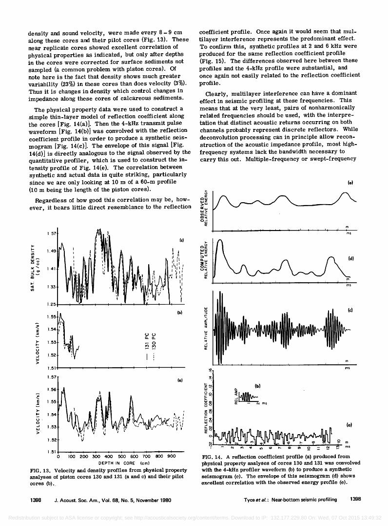
density and sound velocity, were made every 8-9 cm along these cores and their pilot cores (Fig. 13). These near replicate cores showed excellent correlation of physical properties as indicated, but only after depths in the cores were corrected for surface sediments not sampled (a common problem with piston cores). Of note here is the fact that density shows much greater variability (23%) in these cores than does velocity (3%). Thus it is changes in density which control changes in impedance along these cores of calcareous sediments.

The physical property data were used to construct a simple thin-layer model of reflection coefficient along the cores [Fig. 14(a)]. Then the 4-kHz transmit pulse waveform [Fig. 14(b)] was convolved with the reflection coefficient profile in order to produce a synthetic seis- toogram [Fig. 14(c)]. The envelope of this signal [Fig. 14(d)] is directly analogous to the signal observed by the quantitative profiler, which is used to construct the intensity profile of Fig. 14(e). The correlation between synthetic and actual data is quite striking, particularly since we are only looking at 10 m of a 60-m profile (10 m being the length of the piston cores).

Regardless of how good this correlation may be, however, it bears little direct resemblance to the reflection

.49

141

1 33

1251

1.55

'•' 1.54 E

>' 1.53

0 j 1.52

1.51

1'57 l 1.56'

E 1 .55

•- 1.54

0

-'l 1.53,

1.52'

1.51 0 t I I I I I I I I

100 200 300 400 500 600 700 800 900

DEPTH IN CORE (cm)

FIG. 13. Velocity and density profiles from physical property analyses of piston cores 130 and 131 (a and c) and their pilot cores (b).

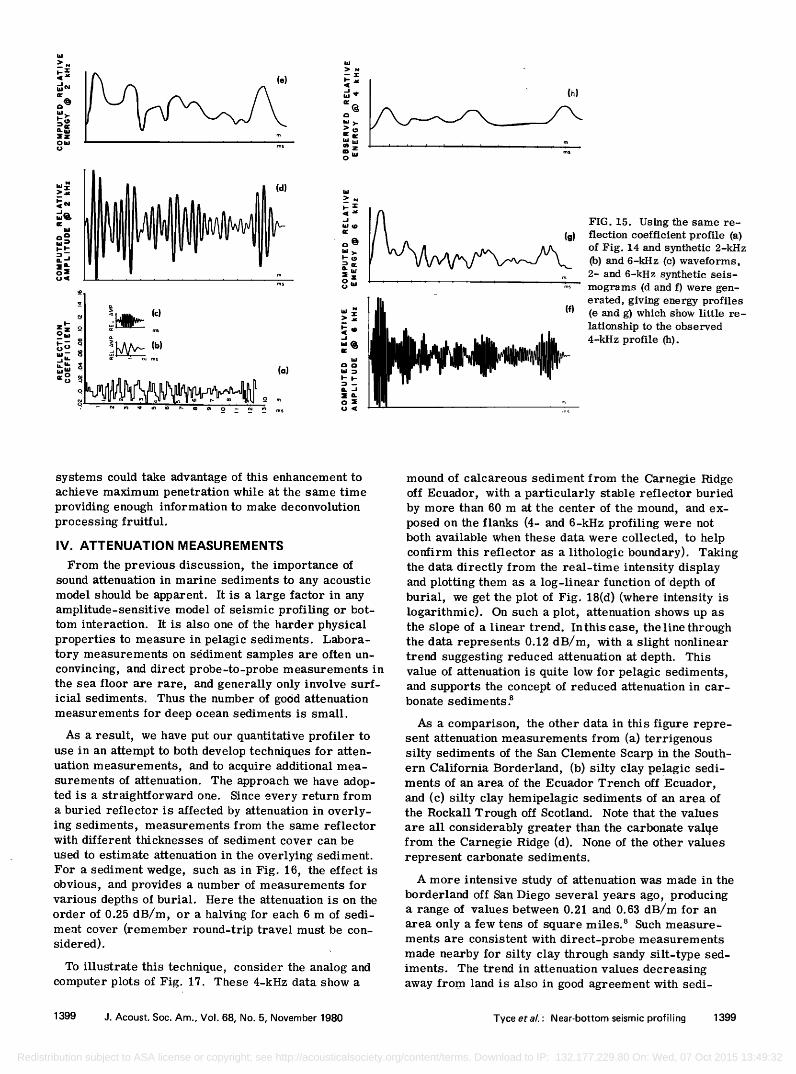
coefficient profile. Once again it would seem that multilayer interference represents the predominant effect. To confirm this, synthetic profiles at 2 and 6 kHz were produced for the same reflection coefficient profile (Fig. 15). The differences observed here between these profiles and the 4-kHz profile were substantial, and once again not easily related to the reflection coefficient profile.

Clearly, multilayer interference can have a dominant effect in seismic profiling at these frequencies. This means that at the very least, pairs of nonharmonically related frequencies should be used, with the interpre- tation that distinct acoustic returns occurring on both

channels probably represent discrete reflectors. While deconvolution processing can in principle allow recon- struction of the acoustic impedance profile, most high- frequency systems lack the bandwidth necessary to carry this out. Multiple-frequency or swept-frequency

(e)

bjz

o•

i-z

:•> O•

ms

z _•

L,I.J _

O• n,- • ed ms c) ß

z8 0 ß

• •' (a) _j

•0

.'T- m

FIG. 14. A reflection coefficient profile (a) produced from physical property analyses of cores 130 and 131 was convolved with the 4-kHz profiler waveform (b) to produce a synthetic seismogram (c). The envelope of this seismogram (d) shows excellent correlation with the observed energy profile (e).

1398 J. Acoust. Soc. Am., Vol. 68, No. 5, November 1980 Tyce et aL' Near-bottom seismic profiling 1398


•z• (d)

ms

I•- w

•,• (a) o

, _ _

UJUJ m (/) Z ' - ! - '- :' ' : ' : I, I , ell UJ ms o

a• )

0 w •

. (fi

FIG. 15. Using the same re- fleetion coefficient profile (a) of Fig. 14 and synthetic 2-kHz (b) and 6-kHz (c) waveforms, 2- and 6-kHz synthetic seis- mograms (d and f) were generated, giving energy profiles (e and g) which show little re- lationship to the observed 4-kHz profile (h).

systems could take advantage of this enhancement to achieve maximum penetration while at the same time providing enough information to make deconvolution processing fruitful.

IV. ATTENUATION MEASUREMENTS

From the previous discussion, the importance of sound attenuation in marine sediments to any acoustic model should be apparent. It is a large factor in any amplitude-sensitive model of seismic profiling or bottom interaction. It is also one of the harder physical properties to measure in pelagic sediments. Labora- tory measurements on s•diment samples are often un- convincing, and direct probe-to-probe measurements in the sea floor are rare, and generally only involve surf- icial sediments. Thus the number of good attenuation measurements for deep ocean sediments is small.

As a result, we have put our quantitative profiler to use in an attempt to both develop techniques for attenuation measurements, and to acquire additional measurements of attenuation. The approach we have adop- ted is a straightforward one. Since every return from a buried reflector is affected by attenuation in overlying sediments, measurements from the same reflector with different thicknesses of sediment cover can be

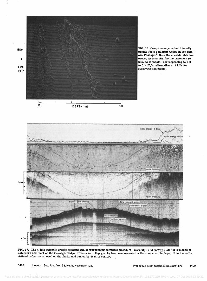
used to estimate attenuation in the overlying sediment. For a sediment wedge, such as in Fig. 16, the effect is obvious, and provides a number of measurements for various depths of burial. Here the attenuation is on the order of 0.25 dB/m, or a halving for each 6 m of sediment cover (remember round-trip travel must be con- sidered).

To illustrate this technique, consider the analog and computer plots of Fig. 17. These 4-kHz data show a

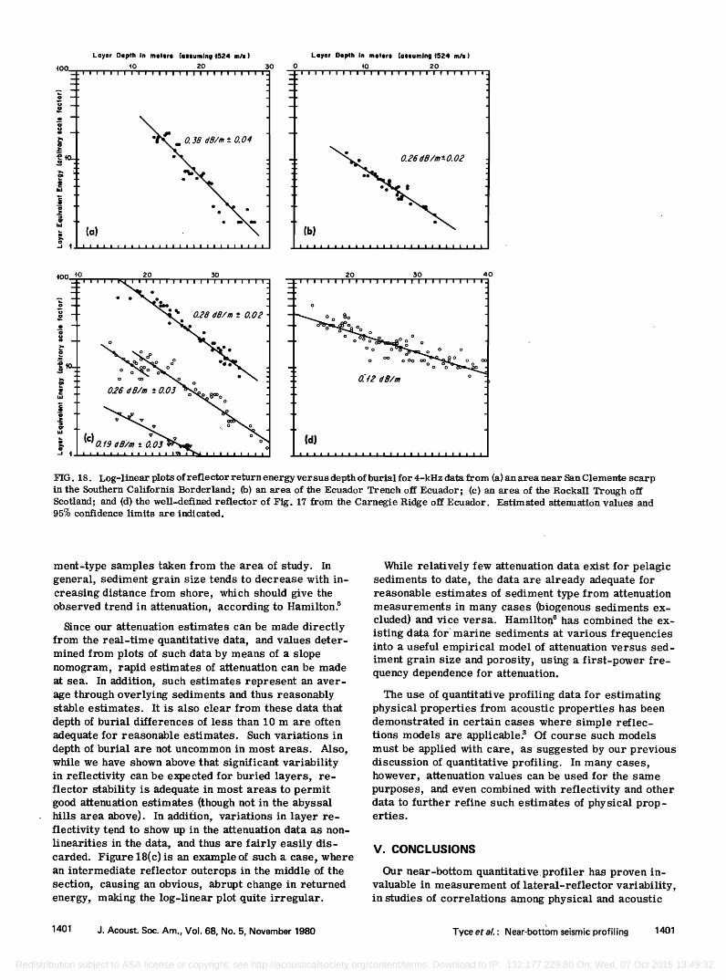
mound of calcareous sediment from the Carnegie Ridge off Ecuador, with a particularly stable reflector buried by more than 60 m at the center of the mound, and ex- posed on the flanks (4- and 6-kHz profiling were not both available when these data were collected, to help confirm this reflector as a lithologic boundary). Taking the data directly from the real-time intensity display and plotting them as a log-linear function of depth of burial, we get the plot of Fig. 18(d) (where intensity is logarithmic). On such a plot, attenuation shows up as the slope of a linear trend. Inthiscase, the line through the data represents 0.12 dB/m, with a slight nonlinear trend suggesting reduced attenuation at depth. This value of attenuation is quite low for pelagic sediments, and supports the concept of reduced attenuation in carbonate sediments. s

As a comparison, the other data in this figure represent attenuation measurements from (a) terrigenous silty sediments of the San Clem ente Scarp in the South- ern California Borderland, (b) silty clay pelagic sediments of an area of the Ecuador Trench off Ecuador, and (c) silty clay hemipelagic sediments of an area of the Rockall Trough off Scotland. Note that the values are all considerably greater than the carbonate val•e from the Carnegie Ridge (d). None of the other values represent carbonate sediments.

A more intensive study of attenuation was made in the borderland off San Diego several years ago, producing a range of values between 0.21 and 0.63 dB/m for an area only a few tens of square miles. 8 Such measurements are consistent with direct-probe measurements made nearby for silty clay through sandy silt-type sediments. The trend in attenuation values decreasing away from land is also in good agreement with sedi-

1399 J. Acoust. Soc. Am., Vol. 68, No. 5, November 1980 Tyce etaL' Near-bottom seismic profiling 1399


Fish

Path

FIG. 16. Computer-equivalent intensity profile for a sediment wedge in the Sam- oan Passage? Note the considerable in- crease in intensity for the basement return as it shoals, corresponding to 0.2 to 0.3 dB/m attenuation at 4 kHz for overlying sediments.

i I i ' • • o DEPTH (m) 50

• ?J .eqUiv. energy O-Sin

-.• ::• ..... • • . ...... . ... • ................ .....• :•.•.-:•':• .•' • ...... •.•.:• •:? .•::• - .................. •:•.•.::... •. • - •.•: .•-•.•--,•,- •,. ,.. -.•:, •,, • . -:..- x ..:•.• - ,:. ,• •, :• t, • • , -, • , • .....

•.- ...• ,::;• .......... •:'-• .•.:::.•:• •.•-•:• •.• ...........

• .................................... •.• .... • ........ • .......... . ...... • ':•::..•¾ ::-•"• :•:- •-• ...... -•.•-: •- .• .... •-•': ........ ...• .- .... •::•--.•::.' • ......... • :• ......... •,-•:• ;-..• • ,"•-"JL"• •'• •:'-•:'• ...... • ......... :•.•.?.• ,• .:•:•:•"•::"'.• ...... ::-'.'•::: " ':•::::•'• -?:• ......... :• • •z:-,•. ' ....... • .... '.•:•,•:'•:• •"•

•.,-," -.':?'•;--...?•:•t:•:?•:?-.•::, % ......... :-.•.:?:-::•.•--:-:• ...... ::;:?"'• .......... :-:?'::'-...-•.-• ..• :,-'?:'2':':"•"•:'; .... -...:• -•. -•: ?:• • :., •:: .: .... .: :•-:•'•'-?•::---.:--.-..• •-:"• .......... L- -: ............ •::.:.:•.. •.•-•.-:'.-.;. ' •-•'• ;-:.•:.:" , ............ : --•- .•..... • •:•: ::..--•.•;"•.•-•:: ...... • .•--•.•:•. •.•: •-•,•-:•"•..•ff.:.:.•::::::•½•:..•....,•.• ::•-::.:•-::•,•.•:•,..• ....•..½• .......... ß •-• • •:•-. •:: :- • ......... .•-. . .•: .- :..,....• . • , .....: .• ...• ß •....-. ,• •.•.•--- •. - ., • -•. : ,•.•:.• .... • .......... •.:..• ............ •. •:•:-.•:.•-..:-.• • ' . •:, ..

...•-.•.... •.•.•-.: - .:.• . .•...•:. %-. -.. , : "• . ........ • •. -• •:5 •: . -•: ..... ;•:.•g• •:. :• .-,•:? .•, .•.:. '• ..::...- .•.. . •.- . •.: • .. -• •..

•o• :•? :':'•. • ':.' :•'"• ..... ' -'• t:- ' I ....... •:i •" ,'• ........ :- .... l ................ ;'• .• :: • . :•-- -• ,½•... - • . - .., -• ..... :•; ;"..• . ::•-i• :•'•:•.- •'. •.•. . .... '•' :'. ;;' :'.: :'-' . ,,.[• '•"' -

..... , .............. .::, ..... . ..................... ...... -• ., w ..... •-' .::.t •::•1•" -•.-: ,. .:•:"' "i •'" ;: :::• .............. ". ....... .•.:.-...:. ....... :•.•:.:

........ : ."...:.:.:.:.:L:.:.::'::.'.':: :::::::::::::::::::::::::: ...... • ........................ .• '•-•:'•i:;.•:'"•:'•::•'•'•"•'•':•"•'•:•k•:...'":::'"' :--:? ' •"-' •' • ..... •--• '•:.: •... •.•'•:?• ....... ':-•'-.•.•?,..: .......... •..•-•: .... ' ..... •:'• -L• .• •:?::•::: .... '"'•:::..• ::'['• ...:: ::.-•:.•. i•.. ....... ::•-:•... :•:•?.• :•:-'.• •.:•ti•'•tio• •gnei:; •:•J• : -• ..• :.

..... .......... ................ ............. •:•::•,... ...: :... ß .•:•..: :..:..-•:•,.?.:::•.:-.:..,• .., •: ..•?.:..:..,.....• •.•,• ' . •.: ..• .......... -•':•:':•' ::'":•:- ......... •'-"•':--.'i'.•. .... -'- "' •. :• •:•-• .... ß ...... •.•-•--.::• .......... . ß •.... " ':'•""::::'• :::.:...:•?)•::'•:•?::•:•:":.' ...... •:.•:': :•':.:• '%-. •'•::.•-.-'-:: •... :•:.•::•:: •..:.:-'" : • •'•:.•:...::%'..•.. •.•. :• ..... - .... •,'"-: " •..•.•::"•,• ....... "•'•:..'t .:-:'•::.•;'•:::-• .... )•':-:•: :•:". .... -•:•:•:.ff:•.•:.-.'•.•:•-:; . ß .......... •,-• •:•-•--:::•.• .... -•:• ......... • -•'••.•-'•.,..•.•, .............................. :.::•:::..•..,•:.•. ............... •..•:•.•:•:•:...•.,..,•:• •;•-. .... •" .• ...... • -"•-•:.• -:-:':"•:•" ::•"•::" ;•::•-:•:•:-'" •:•:;'•' :• '•:;•:• '•: ':•-.•o•t'o.• retura •. ............ ' ...... '• .............. ..•:';' .:. :• ..... ?•-• ...:•;?•'.:• '?•. ...-: ..... :•:.. • •-•::•:•:.. .:-.:c•.::•: ::::; ............. •:.? :•,:z...•,:::•.•-::.::• ..... .... .•. :. ........ •:.:•..:..,•. •,:.•.':•. '.....-.•:-:•::•....•.:•'. ........ •:'• ..:•-•::...:•:• '•:.:. ........................... .. •'•,........ .?:•.:': ..- .................... .•.::•:::-•:--•:... ;•:,•: •:.;:•.•. ..

..,

FIG. 17, •e 4-•z seismic profile •ottom) and corres•nd•g computer pressure, intensity, and energy plots for a mo•d of calcerous sediment on the Ca•egie Ridge off Ecuador. Topography has been removed • the computer displays. Note the well- defied reflector e•osed on the Q•ks and buried by 60 m • center.

1400 J. Acoust. Soc. Am.• Vol. 68, No. 5, November 1980 Tyce et aL' Near-bottom seismic profiling 14OO


400

.• - o -

c

c

Layer Depfh In meters (assuming i$24 m/s) •0 20

I I I I I I I I I I I I I I I I I I I I I I I I I I I

(a) Illalllllllllllllill•11111l

Layer Depth In meters (assuming t524 •o 20

IIIIIIIIIIIIIIIIIlillllllil

•o O. 26 dB/m + O. 02

ltttttilittiilitlltllllllll

4O

FIG. 18. Log-linear plots of reflector return energy versus depth of burial for 4-kHz data from (a) an area near San Clemente scarp in the Southern California Borderland; (b) an area of the Ecuador Trench off Ecuador; (c) an area of the Rockall Trough off Scotland; and (d) the well-defined reflector of Fig. 17 from the Carnegie Ridge off Ecuador. Estimated attenuation values and 95% confidence limits are indicated.

ment-type samples taken from the area of study. In general, sediment grain size tends to decrease w•- .,- creasing distance from shore, which should give the observed trend in attenuation, according to Hamilton. •

Since our attenuation estimates can be made directly from the real-time quantitative data, and values deter- mined from plots of such data by means of a slope homogram, rapid estimates of attenuation can be made at sea. In addition, such estimates represent an aver- •e through overlying sediments and thus reasonably stable estimates. It is also clear from these data that

depth of burial differences of less than 10 m are often •equate for reasonable estimates. Such variations in depth of burial are not uncommon in most areas. Also, while we have shown above that significant variability in reflectivity can be e•ected for buried layers, re- fiector stability is adequate in most areas to permit good affenuation estimates (though not in the abyssal Mlls area above). In addition, variations in layer re- fiectivity tend to show up in the attenuation data as non- linearfries in the data, and thus are fairly easily dis- carded. Fibre 18(c)is an ex•ple of such a case, where an intermediate reflector outcrops in the middle of the section, causing an obvious, abrupt change in returned energy, m•ng the log-linear plot quite irregular.

While relatively few attenuation data exist for pelagic o•,•,,c,• •v date, •,l• u,•a are alrea adequate for reasonable estimates of sediment type from attenuation measurements in many cases (biogenous sediments ex- cluded} and vice versa. Hamilton • has combined the ex- isting data for'marine sediments at various frequencies into a useful empirical model of attenuation versus sediment grain size and porosity, using a first-power frequency dependence for attenuation.

The use of quantitative profiling data for estimating physical properties from acoustic properties has been demonstrated in certain cases where simple reflections models are applicable. • Of course such models must be applied with care, as suggested by our previous discussion of quantitative profiling. In many cases, however, attenuation values can be used for the same purposes, and even combined with reflectivity and other data to further refine such estimates of physical properties.

V. CONCLUSIONS

Our near-bottom quantitative profiler has proven in- valuable in measurement of lateral-reflector variability, in studies of correlations among physical and acoustic

Tyce etaL' Near-bottom seismic profiling 1401 J. Acoust. Soc. Am., Vol. 68, No. 5, November 1980 1401


properties of seafloor sediments, and in efforts to estimate attenuation in different marine sediments.

Near-bottom quantitative profiling has revealed a somewhat unexpected scale of variability in reflectivity of the seafloor and of buried reflectors. The fact that

reflective properties of the seafloor can vary by as much as 10 dB in a few meters laterally implies that local processes have a profound effect on relevant physical properties of the seafloor. The fact that even kilohertz profiler returns are complicated convolutions of transmit waveform and fine-scale vertical layering implies that care must be taken to properly interpret such data, and that multiple-or swept-frequency systems together with deconvolution processing may be required.

However, the fact that attenuation estimates can be made as a valuable by-product of quantitative profiling suggests that lateral variability is not as bad as it may seem. Whenever a stable reflector canbe found beneath

a sediment mound, wedge, or eroded section, attenuation estimates are possibleø Such circumstances appear ,to be relatively common in many parts of the world' s oceans.

Such estimates are already useful for remote predic- tion of general sediment type for nonbiogenous sediments. But the data base for such predictions is very limited. Attenuation values together with physical property measurements are badly needed for most seafloor sediment types, and for biogenous sediments in particular. More routine quantitative profiling, particularly from surface ships, together with sediment sampling is needed to accumulate such data.

ACKNOWLEDGMENTS

This work represents the efforts of a great number of people at the Scripps Institution of Oceanography, and the Marine Physical Laboratory in particular, over the past few years. The Deep Tow engineering group under D. E. Boegeman was essential to the success of these endeavors. Support was provided by the Office of Naval Research, Codes 480 and 220.

iF. N. Spiess and R. C. Tyce, "Marine Physical Laboratory Deep Tow Instrumentation System," Scripps Institution of Oceanography Reference 73-4 (1973).

2R. C. Tyce, "Toward a Quantitative Near-Bottom Seismic Profiler," Oceanogr. Eng. 4, 113-140 (1977).

3L. R. Breslau, "The Normally Incident Reflectivity of the Seafloor at 12 KC and its Correlation with Physical and Geo- logical Properties of Naturally Occurhug Sediments," Woods Hole Oceanographic Institution Reference 67-16 (1967).

4L. C. Breaker, and R. S. Winokur, "The Variability of Bot- tom Reflected Signals Using the Deep Research Vessel AL- VIN," U.S. Naval Oceanographic Internal Office Internal Ref- erence No. 67-92 (1967).

5R. C. Tyce, "Near-Bottom Observations of 4kHz Acoustic Reflectivity and Attenuation," Geophysics 41, 673-699 (1976).

•E. L. Hamilton, "Compressional-Wave Attenuation in Marhue Sediments," Geophysics 37, 620-646 (1972).

?L. Mayer, "Deep Sea Carbonates: Acoustic, Physicalsand Stratigraphic Properties," J. Sediment. Petrol. 49, 819-836 (1979).

8R. C. Tyce, "Estimating Acoustic Attenuation from a Quanti- tative Seismic Profiler," Geophysics (in press).

1402 J. Acoust. Soc. Am., Vol. 68, No. 5, November 1980 Tyceetal.: Near-bottom seismic profiling 1402


Documents

Near-bottom seismic profiling: High lateral variability