NET-VISA: Network Processing Vertically …russell/papers/bssa-netvisa.pdfNET-VISA: Network Processing Vertically Integrated Seismic Analysis ... A Bayesian seismic monitoring system,

NET-VISA: Network Processing Vertically Integrated Seismic Analysis

by Nimar S. Arora, Stuart Russell,* and Erik Sudderth

Abstract The automated processing of multiple seismic signals to detect and local-ize seismic events is a central tool in both geophysics and nuclear treaty verification.This paper reports on a project begun in 2009 to reformulate this problem in a Bayesianframework. A Bayesian seismic monitoring system, NET-VISA, has been built com-prising a spatial event prior and generative models of event transmission and detection,aswell as an inference algorithm. The probabilisticmodel allows for seamless integrationof various disparate sources of information. Applied in the context of the InternationalMonitoring System (IMS), a global sensor network developed for the ComprehensiveNuclear Test Ban Treaty (CTBT), NET-VISA achieves a reduction of around 60% inthe number of missed events compared with the currently deployed system. It also findsevents that are missed by the human analysts who postprocess the IMS output.

Introduction

The Comprehensive Nuclear Test Ban Treaty (CTBT),which bans all nuclear explosions on Earth, is gaining re-newed attention in light of growing worldwide interest inmitigating the risks of nuclear weapons proliferation andtesting. To monitor compliance with the treaty, the Prepara-tory Commission for the Comprehensive Nuclear Test BanTreaty Organization (CTBTO) has installed a suite of sensorsknown as the International Monitoring System (IMS). TheIMS includes waveform sensor stations (seismic, hydroa-coustic, and infrasound) connected by a worldwide commu-nications network to a centralized processing system in theInternational Data Center (IDC) in Vienna. The IDC operatescontinuously and in real time, performing station processing(analysis and reduction of raw seismic sensor data to detectand classify signal arrivals at each station) and networkprocessing (association of signals from different stations thathave presumably come from the same event). Perfect perfor-mance remains well beyond the reach of current technology:the IDC’s automated system, a highly complex and well-tuned piece of software, misses nearly one-third of all seis-mic events in the magnitude range of interest, and about halfof the reported events are spurious. A large team of expertanalysts postprocesses the automatic bulletins to improvetheir accuracy to acceptable levels.

The IDC results indicate that the network processingproblem is far from trivial. There are three primary sourcesof difficulty: (1) the travel time between any two points onEarth and the attenuation of various frequencies and wavetypes are not known accurately; (2) each detector is subjectto local noise that may mask true signals and cause false

detections (as much as 90% of all detections are false); and(3) many thousands of detections are recorded per day, so theproblem of proposing and comparing possible events (sub-sets of detections) is daunting. These considerations suggestthat an approach based on probabilistic inference and com-bination of evidence might be effective, and this paper dem-onstrates that this is in fact the case. For example, such anapproach automatically takes into account nondetections asnegative evidence for a hypothesized event, something thatclassical methods typically do not do.

The existing network processing algorithm in use at theIDC, known as global association (GA) (Le Bras et al., 1994),uses various heuristics to cluster arrivals, and then deter-mines the location of the event in each cluster. The eventlocation algorithm is based on the original iterative linearleast squares method of Geiger (1910, 1912). Of course, thealgorithm has been enhanced considerably over the years, forexample, by the use of singular value decomposition to solvethe resulting matrix equations (Menke, 1989; Lay and Wal-lace, 1995) and by the use of azimuth and slowness to con-strain the solution (Magotra et al., 1987; Roberts et al., 1989).However, in the words of Myers et al. (2007) (p. 1049), “Seis-mic event location is—at its core—a minimization of the dif-ference between observed and predicted arrival times.”Further, all of these classical methods rely only on the asso-ciated arrivals to locate an event. Even the multiple-eventlocation algorithms, such as those due to Waldhauser andEllsworth (2000) and Myers et al. (2007), ignore data fromstations that fail to detect an event.

In this paper, we present a probabilistic model of seismicevent occurrence, Pθ (see Table 1 for a list of all mathemati-cal notations), and another probabilistic model of seismicdetections triggered by events (or noise), Pϕ. We also de-scribe how the model parameters θ and ϕ are estimated from

*Also at Bayesian Logic, Inc., 32432 Lighthouse Way, Union City,California 94587.

1

Bulletin of the Seismological Society of America, Vol. 103, No. 2a, pp. –, , doi: 10.1785/0120120107

historical data and present an algorithm that infers the set ofseismic events given the observed detections. In simple terms,let X be a random variable ranging over all possible collec-tions of seismic events, with each event defined by time, lo-cation, depth, and magnitude. Let Y range over all possiblesignal observations at all seismic stations. Then Pθ�X� de-scribes a parameterized generative prior over events, andPϕ�YjX� describes how the signal is propagated and measured(including travel time, selective absorption and scattering,noise, artifacts, sensor bias, sensor failures, etc.). Given ob-servations Y � y, we are interested in the posterior distribu-tion over events, P�XjY � y�, which is given by Bayes rule:

EQ-TARGET;temp:intralink-;;55;124 P�XjY � y� ∝ Pθ�X�Pϕ�Y � yjX�:For the CTBT monitoring application, we are interested in thevalue x� that maximizes this expression, that is, the mostlikely explanation for all the sensor readings:

EQ-TARGET;temp:intralink-;;313;468 x� � argmaxx

Pθ�X � x�Pϕ�Y � yjX � x�:

Assuming that an algorithm can be devised to solve thisoptimization problem, which turns out to be nontrivial, thekey determinant of the success of the Bayesian approach isthe accuracy of the probability models Pθ and Pϕ. Thesemodels embody, in explicit form, elementary knowledge ofseismology and seismometry, as well as the residual uncer-tainty inherent in that knowledge. Adding to and refining theknowledge embodied in the models reduces residual uncer-tainty and improves system performance.

Many other researchers have previously applied Baye-sian techniques to geophysical problems (see Duijndam,1988a,b for examples). Most of these applications involve in-ference over a fixed set of continuous-valued parameters; theevent localization problem in particular is addressed byMyerset al. (2007). The full monitoring problem involves inferenceover a combinatorial discrete space (the number of events andthe association between events and observations), as well as acontinuous parameter space for each event. In this respect, itresembles the data association problems arising in multitargettracking (Bar-Shalom and Fortmann, 1988).

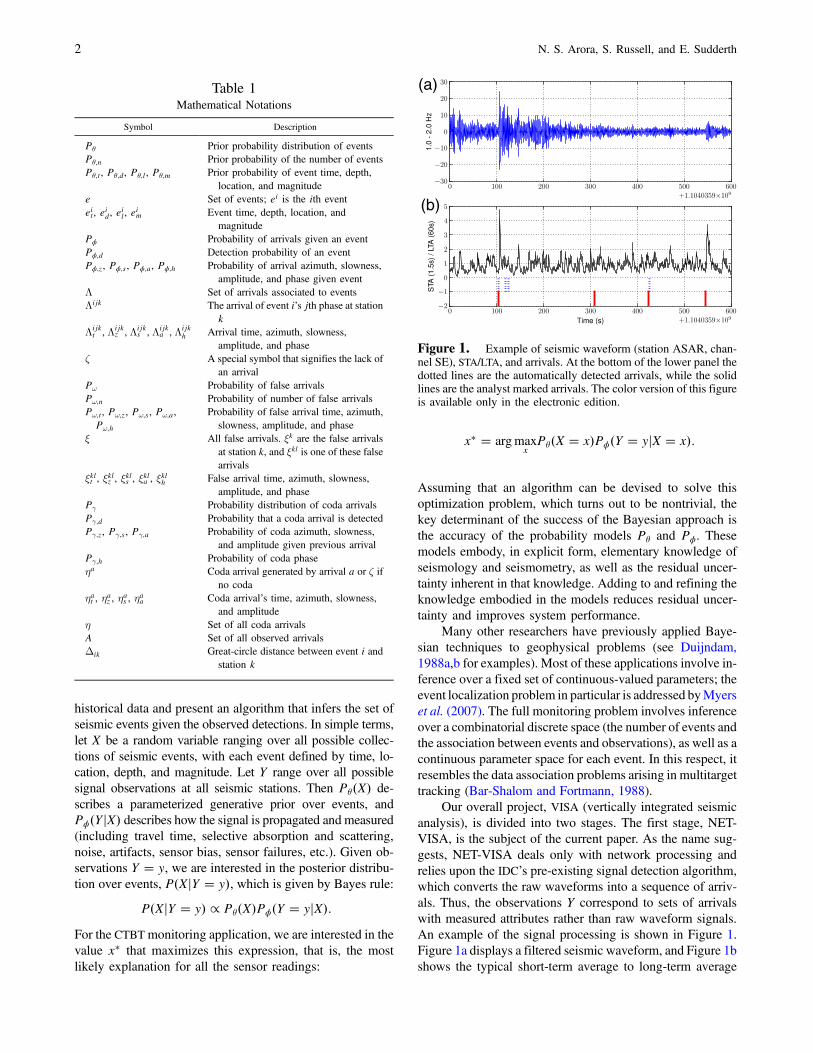
Our overall project, VISA (vertically integrated seismicanalysis), is divided into two stages. The first stage, NET-VISA, is the subject of the current paper. As the name sug-gests, NET-VISA deals only with network processing andrelies upon the IDC’s pre-existing signal detection algorithm,which converts the raw waveforms into a sequence of arriv-als. Thus, the observations Y correspond to sets of arrivalswith measured attributes rather than raw waveform signals.An example of the signal processing is shown in Figure 1.Figure 1a displays a filtered seismic waveform, and Figure 1bshows the typical short-term average to long-term average

Table 1Mathematical Notations

Symbol Description

Pθ Prior probability distribution of eventsPθ;n Prior probability of the number of eventsPθ;t, Pθ;d, Pθ;l, Pθ;m Prior probability of event time, depth,

location, and magnitudee Set of events; ei is the ith eventeit, eid, e

il, e

im Event time, depth, location, and

magnitudePϕ Probability of arrivals given an eventPϕ;d Detection probability of an eventPϕ;z, Pϕ;s, Pϕ;a, Pϕ;h Probability of arrival azimuth, slowness,

amplitude, and phase given eventΛ Set of arrivals associated to eventsΛijk The arrival of event i’s jth phase at station

kΛijkt , Λijk

z , Λijks , Λijk

a , Λijkh Arrival time, azimuth, slowness,

amplitude, and phaseζ A special symbol that signifies the lack of

an arrivalPω Probability of false arrivalsPω;n Probability of number of false arrivalsPω;t, Pω;z, Pω;s, Pω;a,Pω;h

Probability of false arrival time, azimuth,slowness, amplitude, and phase

ξ All false arrivals. ξk are the false arrivalsat station k, and ξkl is one of these falsearrivals

ξklt , ξklz , ξkls , ξkla , ξklh False arrival time, azimuth, slowness,amplitude, and phase

Pγ Probability distribution of coda arrivalsPγ;d Probability that a coda arrival is detectedPγ;z, Pγ;s, Pγ;a Probability of coda azimuth, slowness,

and amplitude given previous arrivalPγ;h Probability of coda phaseηa Coda arrival generated by arrival a or ζ if

no codaηat , ηaz , ηas , ηaa Coda arrival’s time, azimuth, slowness,

and amplitudeη Set of all coda arrivalsA Set of all observed arrivalsΔik Great-circle distance between event i and

station k

(a)

(b)

Figure 1. Example of seismic waveform (station ASAR, chan-nel SE), STA/LTA, and arrivals. At the bottom of the lower panel thedotted lines are the automatically detected arrivals, while the solidlines are the analyst marked arrivals. The color version of this figureis available only in the electronic edition.

2 N. S. Arora, S. Russell, and E. Sudderth

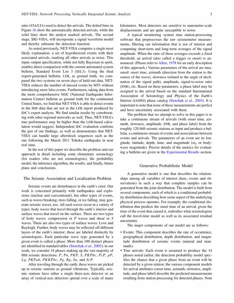
ratio (STA/LTA) used to detect the arrivals. The dotted lines inFigure 1b show the automatically detected arrivals, while thesolid lines show the analyst marked arrivals. The secondstage, SIG-VISA, will incorporate a signal waveform modeland thereby subsume the detection function.

As noted previously, NET-VISA computes a single mostlikely explanation: a set of hypothesized events with theirassociated arrivals, marking all other arrivals as noise. Thisinput–output specification, while not fully Bayesian in spirit,enables direct comparison with the current automated systembulletin, Standard Event List 3 (SEL3). Using the finalexpert-generated bulletin, LEB, as ground truth, we com-pared the two systems on seven days of held-out data. NET-VISA reduces the number of missed events by 60% withoutintroducing more false events. Furthermore, taking data fromthe more comprehensive NEIC (National Earthquake Infor-mation Center) bulletin as ground truth for the continentalUnited States, we find that NET-VISA is able to detect eventsin the IMS data that are not in the LEB report produced byIDC’s expert analysts. We find similar results by corroborat-ing with other regional networks as well. Thus, NET-VISA’strue performance may be higher than the LEB-based calcu-lation would suggest. Independent IDC evaluation confirmsthe gist of our findings, as well as demonstrates that NET-VISA can handle large aftershock sequences such as theone following the March 2011 Tohoku earthquake in nearreal time.

In the rest of this paper we describe the problem and ourapproach in detail including some elementary seismology(for readers who are not seismologists), the probabilitymodel, the inference algorithm, the results, and finally, futureplans and conclusions.

The Seismic Association and Localization Problem

Seismic events are disturbances in the earth’s crust. Ourwork is concerned primarily with earthquakes and explo-sions (nuclear and conventional), but other types of events,such as waves breaking, trees falling, or ice falling, may gen-erate seismic waves, too. All such waves occur in a variety oftypes: body waves that travel through the earth’s interior andsurface waves that travel on the surface. There are two typesof body waves: compression or P waves and shear or Swaves. There are also two types of surface waves: Love andRayleigh. Further, body waves may be reflected off differentlayers of the earth’s interior; these are labeled distinctly byseismologists. Each particular wave type generated by agiven event is called a phase. More than 100 distinct phasesare identified in standard tables (Storchak et al., 2003); in ourwork, we consider 14 phases making up the vast majority ofIMS seismic detections: P, Pn, PKP, S, PKPbc, PcP, pP,Lg, PKPab, PKKPbc, Pg, Rg, Sn, and ScP.

After traveling through the earth, these waves are pickedup in seismic stations as ground vibrations. Typically, seis-mic stations have either a single three-axis detector or anarray of vertical-axis detectors spread over a scale of many

kilometers. Most detectors are sensitive to nanometer-scaledisplacements and are quite susceptible to noise.

A typical monitoring system runs station-processingsoftware that preprocesses the raw seismometer measure-ments, filtering out information that is not of interest andcomputing short-term and long-term averages of the signalamplitude. When the ratio of these averages exceeds a fixedthreshold, an arrival (also called a trigger or onset) is an-nounced. (Please refer to Allen, 1978 for an early descriptionof this approach.) Various parameters of the arrival are mea-sured: onset time, azimuth (direction from the station to thesource of the wave), slowness (related to the angle of decli-nation of the signal path), amplitude, signal-to-noise ratio(SNR), etc. Based on these parameters, a phase label may beassigned to the arrival based on the standard InternationalAssociation of Seismology and Physics of the Earth’sInterior (IASPEI) phase catalog (Storchak et al., 2003). It isimportant to note that none of these measurements are perfectand have uncertainty associated with them.

The problem that we attempt to solve in this paper is totake a continuous stream of arrivals (with onset time, azi-muth, slowness, amplitude, SNR, and phase label) from theroughly 120 IMS seismic stations as input and produce a bul-letin, a continuous stream of events and associations betweenevents and arrivals. The parameters of an event are its lon-gitude, latitude, depth, time, and magnitude (mb or body-wave magnitude). Precise details of the metrics for evaluat-ing a bulletin are given in the Experimental Results section.

Generative Probabilistic Model

A generative model is one that describes the relation-ships among all variables of interest (here, events and ob-servations) in such a way that complete samples can begenerated from the joint distribution. The model is built fromseveral components, each of which is a conditional probabil-ity distribution describing how some aspect of the underlyingphysical process operates. For example, the conditional dis-tribution that predicts the onset time of an arrival, given thetime of the event that caused it, embodies what seismologistscall the travel-time model as well as its associated residualuncertainty.

The major components of our model are as follows:

• Events: This component describes the rate of occurrence,geographical distribution, depth distribution, and magni-tude distribution of seismic events (natural and man-made).

• True arrivals: Each event is assumed to produce the 14phases noted earlier; the detection probability model spec-ifies the chance that a given phase from an event will bedetected by a given station; the various component modelsfor arrival attributes (onset time, azimuth, slowness, ampli-tude, and phase label) describe the predicted measurementsresulting from station processing for detected phases. Note

NET-VISA: Network Processing Vertically Integrated Seismic Analysis 3

that measurements may include errors; for example, thephase label may not match the actual phase.

• False arrivals: The model describes the rate of false (noise-generated) arrivals at each station and their attribute distri-butions.

• Coda arrivals: Any arrival may trigger further spuriousarrivals detected by the station-processing algorithms inthe coda or tail of the waveform, due to additional peaksin the arriving amplitude. Attributes of coda arrivals areusually correlated with those of the triggering arrival.

The following sections describe these components in de-tail, giving their mathematical forms and methods of param-eter estimation.

Events

In the following, we only consider events with body-wave magnitude mb 2 or higher. All other events are consid-ered noise, because they are too small to be relevant for treatymonitoring purposes.

Event Rate and Time. Events are assumed to be generatedby a time-homogeneous Poisson process with a rate param-eter, λe. If e is a set of events (of size jej), and T is the timeperiod under consideration (in seconds), the prior probabilityof the number of events, Pθ;n�·�, is given by

EQ-TARGET;temp:intralink-;df1;313;673Pθ;n�jej� ��λeT�jej exp�−λeT�

jej! : (1)

For each event, ei, the event time, eit, is uniformly distributedbetween 0 and T; in other words, the prior probability densityof the event time, Pθ;t�·�, is given by

EQ-TARGET;temp:intralink-;df2;313;600Pθ;t�eit� �1

T: (2)

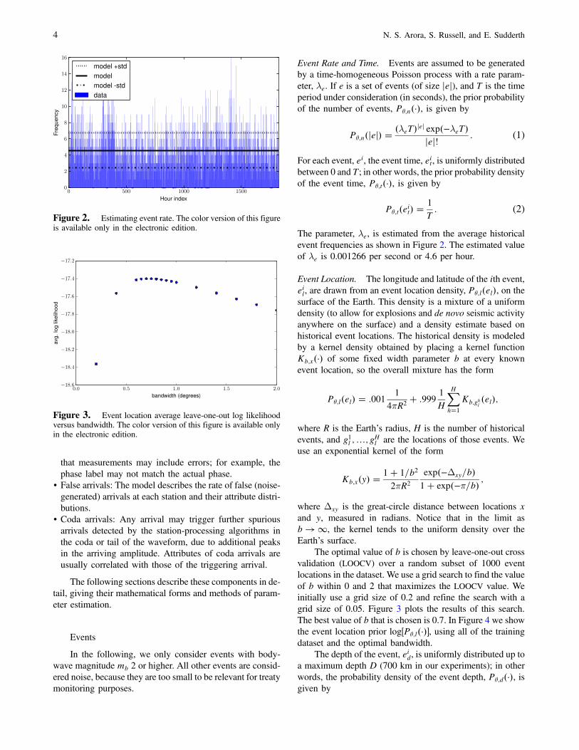
The parameter, λe, is estimated from the average historicalevent frequencies as shown in Figure 2. The estimated valueof λe is 0.001266 per second or 4.6 per hour.

Event Location. The longitude and latitude of the ith event,eil, are drawn from an event location density, Pθ;l�el�, on thesurface of the Earth. This density is a mixture of a uniformdensity (to allow for explosions and de novo seismic activityanywhere on the surface) and a density estimate based onhistorical event locations. The historical density is modeledby a kernel density obtained by placing a kernel functionKb;x�·� of some fixed width parameter b at every knownevent location, so the overall mixture has the form

EQ-TARGET;temp:intralink-;;313;409 Pθ;l�el� � :0011

4πR2� :999

1

H

XHh�1

Kb;ghl�el�;

where R is the Earth’s radius, H is the number of historicalevents, and g1l ;…; gHl are the locations of those events. Weuse an exponential kernel of the form

EQ-TARGET;temp:intralink-;;313;329 Kb;x�y� �1� 1=b2

2πR2

exp�−Δxy=b�1� exp�−π=b� ;

where Δxy is the great-circle distance between locations xand y, measured in radians. Notice that in the limit asb → ∞, the kernel tends to the uniform density over theEarth’s surface.

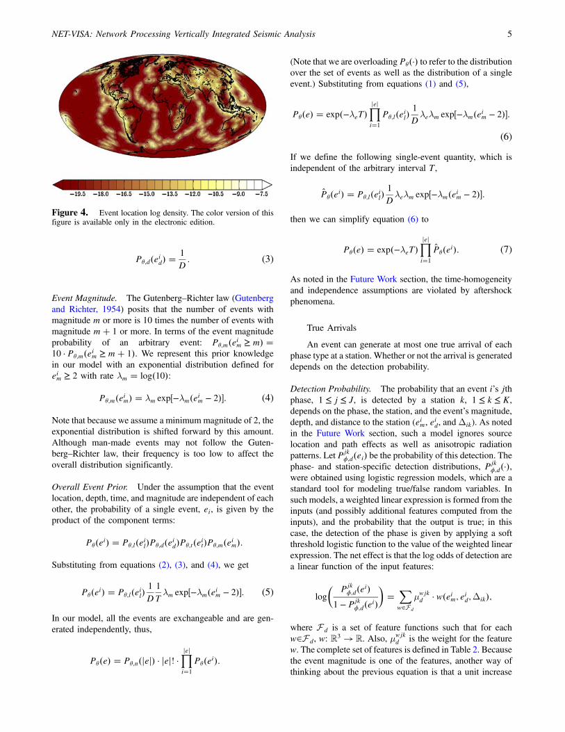
The optimal value of b is chosen by leave-one-out crossvalidation (LOOCV) over a random subset of 1000 eventlocations in the dataset. We use a grid search to find the valueof b within 0 and 2 that maximizes the LOOCV value. Weinitially use a grid size of 0.2 and refine the search with agrid size of 0.05. Figure 3 plots the results of this search.The best value of b that is chosen is 0.7. In Figure 4 we showthe event location prior log�Pθ;l�·��, using all of the trainingdataset and the optimal bandwidth.

The depth of the event, eid, is uniformly distributed up toa maximum depth D (700 km in our experiments); in otherwords, the probability density of the event depth, Pθ;d�·�, isgiven by

Figure 2. Estimating event rate. The color version of this figureis available only in the electronic edition.

Figure 3. Event location average leave-one-out log likelihoodversus bandwidth. The color version of this figure is available onlyin the electronic edition.


EQ-TARGET;temp:intralink-;df3;55;524Pθ;d�eid� �1

D: (3)

Event Magnitude. The Gutenberg–Richter law (Gutenbergand Richter, 1954) posits that the number of events withmagnitude m or more is 10 times the number of events withmagnitude m� 1 or more. In terms of the event magnitudeprobability of an arbitrary event: Pθ;m�eim ≥ m� �10 · Pθ;m�eim ≥ m� 1�. We represent this prior knowledgein our model with an exponential distribution defined foreim ≥ 2 with rate λm � log�10�:

EQ-TARGET;temp:intralink-;df4;55;383Pθ;m�eim� � λm exp�−λm�eim − 2��: (4)

Note that because we assume a minimummagnitude of 2, theexponential distribution is shifted forward by this amount.Although man-made events may not follow the Guten-berg–Richter law, their frequency is too low to affect theoverall distribution significantly.

Overall Event Prior. Under the assumption that the eventlocation, depth, time, and magnitude are independent of eachother, the probability of a single event, ei, is given by theproduct of the component terms:

EQ-TARGET;temp:intralink-;;55;229 Pθ�ei� � Pθ;l�eil�Pθ;d�eid�Pθ;t�eit�Pθ;m�eim�:

Substituting from equations (2), (3), and (4), we get

EQ-TARGET;temp:intralink-;df5;55;183Pθ�ei� � Pθ;l�eil�1

D1

Tλm exp�−λm�eim − 2��: (5)

In our model, all the events are exchangeable and are gen-erated independently, thus,

EQ-TARGET;temp:intralink-;;55;116 Pθ�e� � Pθ;n�jej� · jej! ·Yjeji�1

Pθ�ei�:

(Note that we are overloading Pθ�·� to refer to the distributionover the set of events as well as the distribution of a singleevent.) Substituting from equations (1) and (5),

EQ-TARGET;temp:intralink-;df6;313;697Pθ�e� � exp�−λeT�Yjeji�1

Pθ;l�eil�1

Dλeλm exp�−λm�eim − 2��:

(6)

If we define the following single-event quantity, which isindependent of the arbitrary interval T,

EQ-TARGET;temp:intralink-;;313;606 P̂θ�ei� � Pθ;l�eil�1

Dλeλm exp�−λm�eim − 2��:

then we can simplify equation (6) to

EQ-TARGET;temp:intralink-;df7;313;551Pθ�e� � exp�−λeT�Yjeji�1

P̂θ�ei�: (7)

As noted in the Future Work section, the time-homogeneityand independence assumptions are violated by aftershockphenomena.

True Arrivals

An event can generate at most one true arrival of eachphase type at a station. Whether or not the arrival is generateddepends on the detection probability.

Detection Probability. The probability that an event i’s jthphase, 1 ≤ j ≤ J, is detected by a station k, 1 ≤ k ≤ K,depends on the phase, the station, and the event’s magnitude,depth, and distance to the station (eim, eid, andΔik). As notedin the Future Work section, such a model ignores sourcelocation and path effects as well as anisotropic radiationpatterns. Let Pjk

ϕ;d�ei� be the probability of this detection. Thephase- and station-specific detection distributions, Pjk

ϕ;d�·�,were obtained using logistic regression models, which are astandard tool for modeling true/false random variables. Insuch models, a weighted linear expression is formed from theinputs (and possibly additional features computed from theinputs), and the probability that the output is true; in thiscase, the detection of the phase is given by applying a softthreshold logistic function to the value of the weighted linearexpression. The net effect is that the log odds of detection area linear function of the input features:

EQ-TARGET;temp:intralink-;;313;180 log�

Pjkϕ;d�ei�

1 − Pjkϕ;d�ei�

��

Xw∈F d

μwjkd · w�eim; eid;Δik�;

where F d is a set of feature functions such that for eachw∈F d, w: R3 → R. Also, μwjk

d is the weight for the featurew. The complete set of features is defined in Table 2. Becausethe event magnitude is one of the features, another way ofthinking about the previous equation is that a unit increase

Figure 4. Event location log density. The color version of thisfigure is available only in the electronic edition.


in the event magnitude would result in the odds of detectionincreasing by a multiplicative constant. The exact constant isthe exponentiation of the corresponding weight of the mag-nitude feature, and this is station dependent. In fact, if theweight was negative then the detections odds would de-crease; this is, in fact, the case for the travel-time feature.

Directly estimating the feature weights μwjkd is not

always possible because many of the station–phase combi-nations have very little data. To deal with this data sparsitywe used a hierarchical Bayesian procedure (Gelman et al.,2004), which posits that the weight for a station–phase isdrawn from a global prior for that phase. This global prioris, in turn, drawn from a weakly informative prior, as follows:

EQ-TARGET;temp:intralink-;;55;306 μwjkd ∼N �μwj

d ; σwjd � μwj

d ∼N �0; 100��σwj

d �−2 ∼ Γ�0:01; 100�;

where N and Γ are the Gaussian and the gamma distribu-tions parameterized by their mean and standard deviation,and shape and scale, respectively. Estimation of parametersfollows a coordinate ascent procedure. For each phase j, weinitialize μwj

d � 0 and σwjd � 1, and then alternately optimize

μwjkd :∀w, k, μwj

d :∀w, and σwjd :∀w until convergence. In each

maximization step, the optimal value of μwjkd is computed by

second-order optimization, while the remaining values havea closed-form solution.

For each phase, the previously described procedureensures that if a station has a lot of data (both detectionsand nondetections), then its feature weights will be deter-mined almost entirely by its own data, whereas featureweights for data-poor stations tend toward a global averageobtained from all stations. Thus, if most data-rich stations

have a positive weight for event magnitude for the P phase,then a station with very little data will also have a positiveweight for this feature.

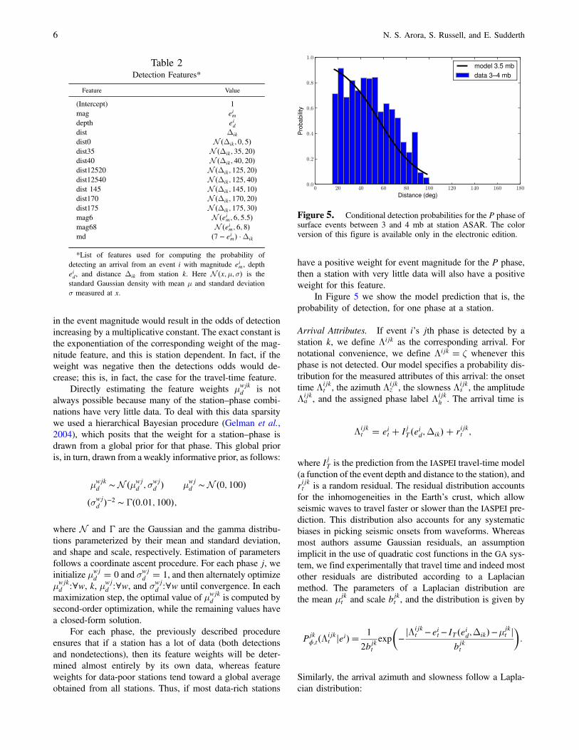
In Figure 5 we show the model prediction that is, theprobability of detection, for one phase at a station.

Arrival Attributes. If event i’s jth phase is detected by astation k, we define Λijk as the corresponding arrival. Fornotational convenience, we define Λijk � ζ whenever thisphase is not detected. Our model specifies a probability dis-tribution for the measured attributes of this arrival: the onsettime Λijk

t , the azimuth Λijkz , the slowness Λijk

s , the amplitudeΛijka , and the assigned phase label Λijk

h . The arrival time is

EQ-TARGET;temp:intralink-;;313;367 Λijkt � eit � IjT�eid;Δik� � rijkt ;

where IjT is the prediction from the IASPEI travel-time model(a function of the event depth and distance to the station), andrijkt is a random residual. The residual distribution accountsfor the inhomogeneities in the Earth’s crust, which allowseismic waves to travel faster or slower than the IASPEI pre-diction. This distribution also accounts for any systematicbiases in picking seismic onsets from waveforms. Whereasmost authors assume Gaussian residuals, an assumptionimplicit in the use of quadratic cost functions in the GA sys-tem, we find experimentally that travel time and indeed mostother residuals are distributed according to a Laplacianmethod. The parameters of a Laplacian distribution arethe mean μjk

t and scale bjkt , and the distribution is given by

EQ-TARGET;temp:intralink-;;313;176 Pjkϕ;t�Λijk

t jei�� 1

2bjktexp

�−jΛijk

t −eit− IT�eid;Δik�−μjkt j

bjkt

�:

Similarly, the arrival azimuth and slowness follow a Lapla-cian distribution:

Table 2Detection Features*

Feature Value

(Intercept) 1mag eimdepth eiddist Δik

dist0 N �Δik; 0; 5�dist35 N �Δik; 35; 20�dist40 N �Δik; 40; 20�dist12520 N �Δik; 125; 20�dist12540 N �Δik; 125; 40�dist 145 N �Δik; 145; 10�dist170 N �Δik; 170; 20�dist175 N �Δik; 175; 30�mag6 N �eim; 6; 5:5�mag68 N �eim; 6; 8�md �7 − eim� ·Δik

*List of features used for computing the probability ofdetecting an arrival from an event i with magnitude eim, deptheid, and distance Δik from station k. Here N �x;μ;σ� is thestandard Gaussian density with mean μ and standard deviationσ measured at x.

Figure 5. Conditional detection probabilities for the P phase ofsurface events between 3 and 4 mb at station ASAR. The colorversion of this figure is available only in the electronic edition.


EQ-TARGET;temp:intralink-;;313;733 Pjkϕ;z�Λijk

z jei� � 1

2bjkzexp

�−jψ�Λijk

z ; Gz�skl ; eil�� − μjkz j

bjkz

�;

Pjkϕ;s�Λijk

s jei� � 1

2bjksexp

�−jΛijk

s − Ijs�eid;Δik� − μjks j

bjks

�:

Here the function ψ computes the difference in the observedangle Λijk

z and the angle computed from the geographicalfunction Gz, which depends on the station location, skl , andthe event location, eil. Also, I

js is the slowness value com-

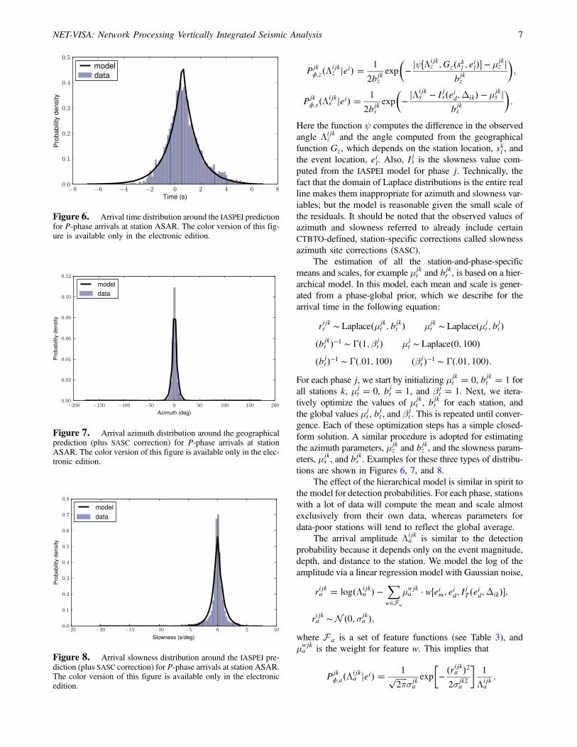
puted from the IASPEI model for phase j. Technically, thefact that the domain of Laplace distributions is the entire realline makes them inappropriate for azimuth and slowness var-iables; but the model is reasonable given the small scale ofthe residuals. It should be noted that the observed values ofazimuth and slowness referred to already include certainCTBTO-defined, station-specific corrections called slownessazimuth site corrections (SASC).

The estimation of all the station-and-phase-specificmeans and scales, for example μjk

t and bjkt , is based on a hier-archical model. In this model, each mean and scale is gener-ated from a phase-global prior, which we describe for thearrival time in the following equation:

EQ-TARGET;temp:intralink-;;313;465 rijkt ∼ Laplace�μjkt ; b

jkt � μjk

t ∼ Laplace�μjt ; b

jt �

�bjkt �−1 ∼ Γ�1; βjt � μj

t ∼ Laplace�0; 100��bjt �−1 ∼ Γ�:01; 100� �βj

t �−1 ∼ Γ�:01; 100�:For each phase j, we start by initializing μjk

t � 0, bjkt � 1 forall stations k, μj

t � 0, bjt � 1, and βjt � 1. Next, we itera-

tively optimize the values of μjkt , b

jkt for each station, and

the global values μjt , b

jt , and β

jt . This is repeated until conver-

gence. Each of these optimization steps has a simple closed-form solution. A similar procedure is adopted for estimatingthe azimuth parameters, μjk

z and bjkz , and the slowness param-eters, μjk

s , and bjks . Examples for these three types of distribu-

tions are shown in Figures 6, 7, and 8.The effect of the hierarchical model is similar in spirit to

the model for detection probabilities. For each phase, stationswith a lot of data will compute the mean and scale almostexclusively from their own data, whereas parameters fordata-poor stations will tend to reflect the global average.

The arrival amplitude Λijka is similar to the detection

probability because it depends only on the event magnitude,depth, and distance to the station. We model the log of theamplitude via a linear regression model with Gaussian noise,

EQ-TARGET;temp:intralink-;;313;188 rijka � log�Λijka � −

Xw∈F a

μwjka · w�eim; eid; IjT�eid;Δik��;

rijka ∼N �0; σjka �;

where F a is a set of feature functions (see Table 3), andμwjka is the weight for feature w. This implies that

EQ-TARGET;temp:intralink-;;313;111 Pjkϕ;a�Λijk

a jei� � 1��2π

pσjkaexp

�−�rijka �22σjk2

a

�1

Λijka

:

Figure 6. Arrival time distribution around the IASPEI predictionfor P-phase arrivals at station ASAR. The color version of this fig-ure is available only in the electronic edition.

Figure 7. Arrival azimuth distribution around the geographicalprediction (plus SASC correction) for P-phase arrivals at stationASAR. The color version of this figure is available only in the elec-tronic edition.

Figure 8. Arrival slowness distribution around the IASPEI pre-diction (plus SASC correction) for P-phase arrivals at station ASAR.The color version of this figure is available only in the electronicedition.


In order to estimate the feature weights, we use a hierarchicalmodel, as before, which assumes that for each phase the fea-ture weights at a station are drawn from a global prior:

EQ-TARGET;temp:intralink-;;55;562 μwjka ∼N �μwj

a ; σwja � �σjk

a �−2 ∼ Γ�100; βja�

μwja ∼N �0; 100� �σwj

a �−2 ∼ Γ�:01; 100��βj

a�−1 ∼ Γ�:01; 100�:

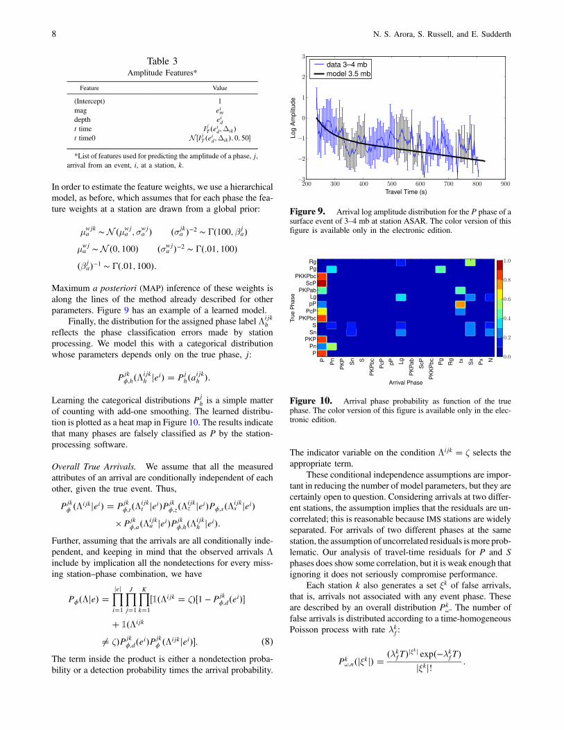
Maximum a posteriori (MAP) inference of these weights isalong the lines of the method already described for otherparameters. Figure 9 has an example of a learned model.

Finally, the distribution for the assigned phase label Λijkh

reflects the phase classification errors made by stationprocessing. We model this with a categorical distributionwhose parameters depends only on the true phase, j:

EQ-TARGET;temp:intralink-;;55;404 Pjkϕ;h�Λijk

h jei� � Pjh�aijkh �:

Learning the categorical distributions Pjh is a simple matter

of counting with add-one smoothing. The learned distribu-tion is plotted as a heat map in Figure 10. The results indicatethat many phases are falsely classified as P by the station-processing software.

Overall True Arrivals. We assume that all the measuredattributes of an arrival are conditionally independent of eachother, given the true event. Thus,EQ-TARGET;temp:intralink-;;55;260

Pjkϕ �Λijkjei� � Pjk

ϕ;t�Λijkt jei�Pjk

ϕ;z�Λijkz jei�Pϕ;s�Λijk

s jei�× Pjk

ϕ;a�Λijka jei�Pjk

ϕ;h�Λijkh jei�:

Further, assuming that the arrivals are all conditionally inde-pendent, and keeping in mind that the observed arrivals Λinclude by implication all the nondetections for every miss-ing station–phase combination, we have

EQ-TARGET;temp:intralink-;df8;55;168Pϕ�Λje� �Yjeji�1

YJj�1

YKk�1

�1�Λijk � ζ��1 − Pjkϕ;d�ei��

� 1�Λijk

≠ ζ�Pjkϕ;d�ei�Pjk

ϕ �Λijkjei��: (8)

The term inside the product is either a nondetection proba-bility or a detection probability times the arrival probability.

The indicator variable on the condition Λijk � ζ selects theappropriate term.

These conditional independence assumptions are impor-tant in reducing the number of model parameters, but they arecertainly open to question. Considering arrivals at two differ-ent stations, the assumption implies that the residuals are un-correlated; this is reasonable because IMS stations are widelyseparated. For arrivals of two different phases at the samestation, the assumption of uncorrelated residuals ismore prob-lematic. Our analysis of travel-time residuals for P and Sphases does show some correlation, but it is weak enough thatignoring it does not seriously compromise performance.

Each station k also generates a set ξk of false arrivals,that is, arrivals not associated with any event phase. Theseare described by an overall distribution Pk

ω. The number offalse arrivals is distributed according to a time-homogeneousPoisson process with rate λkf:

EQ-TARGET;temp:intralink-;;313;105 Pkω;n�jξkj� �

�λkfT�jξ

kj exp�−λkfT�jξkj! :

Table 3Amplitude Features*

Feature Value

(Intercept) 1mag eimdepth eidt time IjT�eid;Δik�t time0 N �IjT�eid;Δik�; 0; 50�

*List of features used for predicting the amplitude of a phase, j,arrival from an event, i, at a station, k.

Figure 9. Arrival log amplitude distribution for the P phase of asurface event of 3–4 mb at station ASAR. The color version of thisfigure is available only in the electronic edition.

Figure 10. Arrival phase probability as function of the truephase. The color version of this figure is available only in the elec-tronic edition.


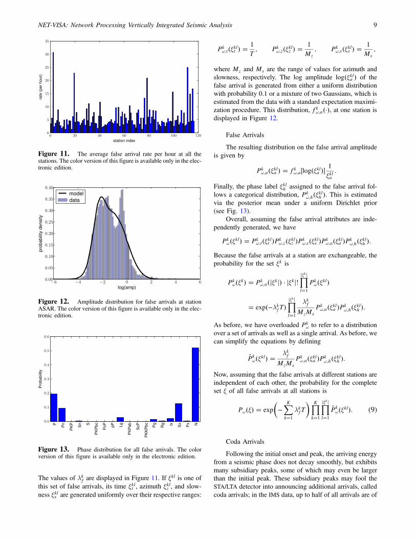
The values of λkf are displayed in Figure 11. If ξkl is one ofthis set of false arrivals, its time ξklt , azimuth ξklz , and slow-ness ξkls are generated uniformly over their respective ranges:

EQ-TARGET;temp:intralink-;;313;733 Pkω;t�ξklt � �

1

T; Pk

ω;z�ξklz � �1

Mz; Pk

ω;s�ξkls � �1

Ms;

where Mz and Ms are the range of values for azimuth andslowness, respectively. The log amplitude log�ξkla � of thefalse arrival is generated from either a uniform distributionwith probability 0.1 or a mixture of two Gaussians, which isestimated from the data with a standard expectation maximi-zation procedure. This distribution, fkω;a�·�, at one station isdisplayed in Figure 12.

False Arrivals

The resulting distribution on the false arrival amplitudeis given by

EQ-TARGET;temp:intralink-;;313;561 Pkω;a�ξkla � � fkω;a�log�ξkla ��

1

ξkla:

Finally, the phase label ξklh assigned to the false arrival fol-lows a categorical distribution, Pk

ω;h�ξklh �. This is estimatedvia the posterior mean under a uniform Dirichlet prior(see Fig. 13).

Overall, assuming the false arrival attributes are inde-pendently generated, we have

EQ-TARGET;temp:intralink-;;313;455 Pkω�ξkl� � Pk

ω;t�ξklt �Pkω;z�ξklz �Pk

ω;s�ξkls �Pkω;a�ξkla �Pk

ω;h�ξklh �:Because the false arrivals at a station are exchangeable, theprobability for the set ξk is

EQ-TARGET;temp:intralink-;;313;402 Pkω�ξk� � Pk

ω;n�jξkj� · jξkj!Yjξkjl�1

Pkω�ξkl�

� exp�−λkfT�Yjξkjl�1

λkfMzMs

Pkω;a�ξkla �Pk

ω;h�ξklh �:

As before, we have overloaded Pkω to refer to a distribution

over a set of arrivals as well as a single arrival. As before, wecan simplify the equations by defining

EQ-TARGET;temp:intralink-;;313;288 P̂kω�ξkl� �

λkfMzMs

Pkω;a�ξkla �Pk

ω;h�ξklh �:

Now, assuming that the false arrivals at different stations areindependent of each other, the probability for the completeset ξ of all false arrivals at all stations is

EQ-TARGET;temp:intralink-;df9;313;215Pω�ξ� � exp�−XKk�1

λkfT�YK

k�1

Yjξkjl�1

P̂kω�ξkl�: (9)

Coda Arrivals

Following the initial onset and peak, the arriving energyfrom a seismic phase does not decay smoothly, but exhibitsmany subsidiary peaks, some of which may even be largerthan the initial peak. These subsidiary peaks may fool theSTA/LTA detector into announcing additional arrivals, calledcoda arrivals; in the IMS data, up to half of all arrivals are of

Figure 11. The average false arrival rate per hour at all thestations. The color version of this figure is available only in the elec-tronic edition.

Figure 12. Amplitude distribution for false arrivals at stationASAR. The color version of this figure is available only in the elec-tronic edition.

Figure 13. Phase distribution for all false arrivals. The colorversion of this figure is available only in the electronic edition.


this type. An example of coda arrivals can be seen in Figure 1around 20 s after the main arrival, which is at offset 100 s.One might imagine that coda arrivals can be lumped in withfalse arrivals, but it turns out that the attributes of coda arriv-als are strongly correlated with those of the triggering arrival.If the coda arrivals are not modeled explicitly, then our in-ference will end up hypothesizing additional spurious eventsas the most likely explanation for many of the coda arrivals.

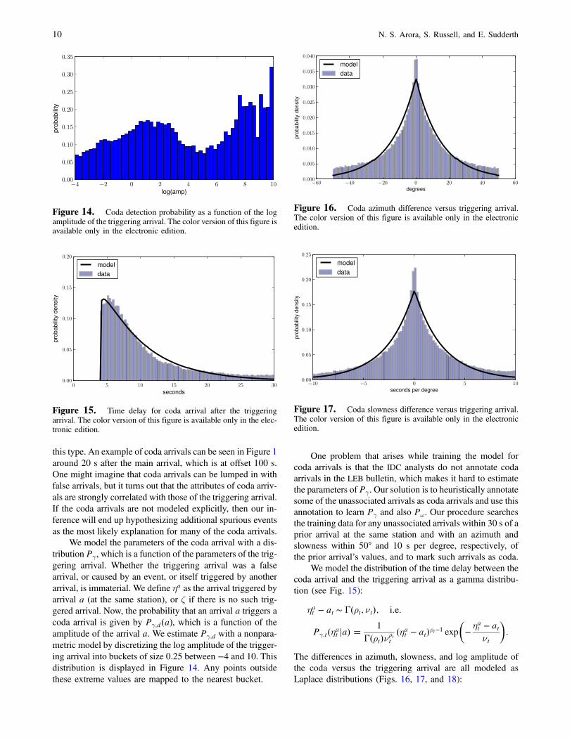
We model the parameters of the coda arrival with a dis-tribution Pγ , which is a function of the parameters of the trig-gering arrival. Whether the triggering arrival was a falsearrival, or caused by an event, or itself triggered by anotherarrival, is immaterial. We define ηa as the arrival triggered byarrival a (at the same station), or ζ if there is no such trig-gered arrival. Now, the probability that an arrival a triggers acoda arrival is given by Pγ;d�a�, which is a function of theamplitude of the arrival a. We estimate Pγ;d with a nonpara-metric model by discretizing the log amplitude of the trigger-ing arrival into buckets of size 0.25 between −4 and 10. Thisdistribution is displayed in Figure 14. Any points outsidethese extreme values are mapped to the nearest bucket.

One problem that arises while training the model forcoda arrivals is that the IDC analysts do not annotate codaarrivals in the LEB bulletin, which makes it hard to estimatethe parameters of Pγ . Our solution is to heuristically annotatesome of the unassociated arrivals as coda arrivals and use thisannotation to learn Pγ and also Pω. Our procedure searchesthe training data for any unassociated arrivals within 30 s of aprior arrival at the same station and with an azimuth andslowness within 50° and 10 s per degree, respectively, ofthe prior arrival’s values, and to mark such arrivals as coda.

We model the distribution of the time delay between thecoda arrival and the triggering arrival as a gamma distribu-tion (see Fig. 15):

EQ-TARGET;temp:intralink-;;313;156 ηat − at ∼ Γ�ρt; νt�; i:e:

Pγ;t�ηat ja� �1

Γ�ρt�νρtt�ηat − at�ρt−1 exp

�−ηat − at

νt

�:

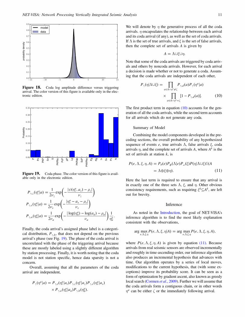
The differences in azimuth, slowness, and log amplitude ofthe coda versus the triggering arrival are all modeled asLaplace distributions (Figs. 16, 17, and 18):

Figure 14. Coda detection probability as a function of the logamplitude of the triggering arrival. The color version of this figure isavailable only in the electronic edition.

Figure 15. Time delay for coda arrival after the triggeringarrival. The color version of this figure is available only in the elec-tronic edition.

Figure 17. Coda slowness difference versus triggering arrival.The color version of this figure is available only in the electronicedition.

Figure 16. Coda azimuth difference versus triggering arrival.The color version of this figure is available only in the electronicedition.


EQ-TARGET;temp:intralink-;;55;326 Pγ;z�ηaz ja� �1

2νzexp

�−jψ�ηaz ; az� − ρzj

νz

�

Pγ;s�ηas ja� �1

2νsexp

�−jηas − as − ρsj

νs

�

Pγ;a�ηaaja� �1

2νaexp

�−j log�ηaa� − log�aa� − ρaj

νa

�1

ηaa:

Finally, the coda arrival’s assigned phase label is a categori-cal distribution, Pγ;h, that does not depend on the previousarrival’s phase (see Fig. 19). The phase of the coda arrival isuncorrelated with the phase of the triggering arrival becausethese are mostly labeled using a slightly different algorithmby station processing. Finally, it is worth noting that the codamodel is not station specific, hence data sparsity is not aconcern.

Overall, assuming that all the parameters of the codaarrival are independent,

EQ-TARGET;temp:intralink-;;55;112

Pγ�ηaja� � Pγ;t�ηat jat�Pγ;z�ηat jaz�Pγ;s�ηas jas�× Pγ;a�ηaajaa�Pγ;h�ηah�:

We will denote by η the generative process of all the codaarrivals. η encapsulates the relationship between each arrivaland its coda arrival (if any), as well as the set of coda arrivals.If Λ is the set of true arrivals, and ξ is the set of false arrivals,then the complete set of arrivals A is given by

EQ-TARGET;temp:intralink-;;313;673 A � Λ∪ξ∪η:Note that some of the coda arrivals are triggered by coda arriv-als and others by noncoda arrivals. However, for each arrivala decision is made whether or not to generate a coda. Assum-ing that the coda arrivals are independent of each other,EQ-TARGET;temp:intralink-;df10;313;598

Pγ�ηjΛ∪ξ� �Y

a∈A∧ηa≠ζPγ;d�a�Pγ�ηaja�

×Y

a∈A∧ηa�ζ�1 − Pγ;d�a��: (10)

The first product term in equation (10) accounts for the gen-eration of all the coda arrivals, while the second term accountsfor all arrivals which do not generate any coda.

Summary of Model

Combining the model components developed in the pre-ceding sections, the overall probability of any hypothesizedsequence of events e, true arrivals Λ, false arrivals ξ, codaarrivals η, and the complete set of arrivals A, where Ak is theset of arrivals at station k, is

EQ-TARGET;temp:intralink-;df11;313;405P�e;Λ; ξ; η; A� � Pθ�e�Pϕ�Λje�Pω�ξ�P�ηjΛ∪ξ�1�A� Λ⊕ξ⊕η�: (11)

Here the last term is required to ensure that any arrival isin exactly one of the three sets Λ, ξ, and η. Other obviousconsistency requirements, such as requiring ξk⊆Ak, are leftout for brevity.

Inference

As noted in the Introduction, the goal of NET-VISA’sinference algorithm is to find the most likely explanationconsistent with the observations,

EQ-TARGET;temp:intralink-;;313;236 arg maxe;Λ;ξ;η

P�e;Λ; ξ; ηjA� � arg maxe;Λ;ξ;η

P�e;Λ; ξ; η; A�;

where P�e;Λ; ξ; η; A� is given by equation (11). Becausearrivals from real seismic sensors are observed incrementallyand roughly in time-ascending order, our inference algorithmalso produces an incremental hypothesis that advances withtime. Our algorithm operates by a series of local moves,modifications to the current hypothesis, that (with some ex-ceptions) improve its probability score. It can be seen as aform of optimization by gradient ascent, also known as greedylocal search (Cormen et al., 2009). Further wewill assume thatthe coda arrivals form a contiguous chain, or in other wordsηa can be either ζ or the immediately following arrival.

Figure 18. Coda log amplitude difference versus triggeringarrival. The color version of this figure is available only in the elec-tronic edition.

Figure 19. Coda phase. The color version of this figure is avail-able only in the electronic edition.


Let MT denote the maximum travel time for any phase.Initially, we start with an event window of size W from t0 �0 to t1 � W, and an arrival window of size W �MT fromt0 � 0 to t2 � W �MT . Then we perform a series of localmoves that add or update events in the event window, deleteexisting events, or classify (as true arrival, false arrival, orcoda arrival) the arrivals in the arrival window. Next, the win-dows are moved forward by a step size, S. At this point,events older than t0 −MT become stable: none of the movesmodify either the events or arrivals associated with them.These events are then output. While in theory this algorithmnever needs to terminate, our experiments continue until thetest dataset is fully consumed.

The algorithm’s initial hypothesis is that all new arrivalsadded to the arrival window are false arrivals. This is refinedby classifying any arrival a (at station k), with the immedi-ately preceding arrival a−, as a coda arrival if

EQ-TARGET;temp:intralink-;;55;529 Pγ;d�a−�Pγ�aja−� > �1 − Pγ;d�a−��Pkω�a�:

In simple terms, the condition expressed in the previousequation states that it is more likely that the arrival a− gen-erated a coda and this coda was a than that a− did not generatea coda and a was a false arrival. This default classification foran arrival is retained whenever it is no longer associated withan event. For convenience we define

EQ-TARGET;temp:intralink-;df12;55;435Υk�a� � maxfPγ;d�a−�Pγ�aja−�;�1 − Pγ;d�a−��Pk

ω�a�g:(12)

Next, the birth move generates new events in the event win-dow. These events are added to the hypothesis with Λijk � ζfor each new event i. Subsequently, we repeat the following Ntimes: one improve-arrival move for each arrival in the arrivalwindow, and one improve-event move for each event in theevent window. Finally, the death move kills some of the events,and we repeat one round of improve-arrival and improve-eventmoves. We describe these steps algorithmically next. The indi-vidual moves will be described in more detail later.

1. t0 � 0; t1 � W; t2 � W �MT .2. Repeat while t0 < max time.

a. Give a default classification to arrivals in t0 to t2.b. Add events from birth move (t0, t1, fa:t0 ≤ at ≤ t2g).c. Repeat N times.

i. For each arrival a, such that t0 ≤ at ≤ t2, improve-arrival (a).

ii. For each event ei, such that t0 ≤ eit ≤ t1, improve-event (ei).

d. For all events ei, death move (ei).e. For each arrival a, such that t0 ≤ at ≤ t2, improve-

arrival (a).f. For each event ei, such that t0 ≤ eit ≤ t1, improve-

event (ei).g. t0� � S, t1� � S, t2� � S.h. Output ei, Λijk for all ei such that eit < t0 −MT .

3. Output any remaining ei.

In order to simplify the computations needed to comparealternate hypotheses, we decompose the overall probabilityof equation (11) into the contribution from each event. Wedefine the score Se of an event as the probability ratio of twohypotheses: one in which the event exists, and another inwhich the event does not exist and all of its associated arriv-als have the default classification (false or coda). If an eventhas score less than 1, an alternative hypothesis in which theevent is deleted clearly has higher probability. Critically, thisevent score is unaffected by other events in the current hy-pothesis. From equations (7), (8), (9), (10), and (12) we have

EQ-TARGET;temp:intralink-;;313;601 Se�ei� � Pθ�ei�YJj�1

YKk�1

�1�Λijk � ζ��1 − Pjk

ϕ;d�ei��

� 1�Λijk ≠ ζ�Pjkϕ;d�ei�Pjk

ϕ �Λijkjei�Υk�Λijk�

�:

Note that the final fraction in the previous equation is a like-lihood ratio comparing interpretations of the same arrival aseither the arrival of event i’s jth phase at station k, or as afalse arrival or a coda arrival. We can further decompose thescore into scores Sd for each arrival. The score of Λijk,defined when Λijk ≠ ζ, is the ratio of the probabilities ofthe hypothesis, where the arrival is associated with phasej of event i at station k versus the default classification.

EQ-TARGET;temp:intralink-;;313;431 Sjkd �Λijkjei� � Pjkϕ;d�ei�

1 − Pjkϕ;d�ei�

Pjkϕ �Λijkjei�Υk�Λijk� :

By definition, any arrival with a score less than 1 is morelikely to be a false or coda arrival. Also, the score of an indi-vidual arrival is independent of other arrivals and events inthe hypothesis. These scores play a key role in the followinglocal search moves.

Birth Move

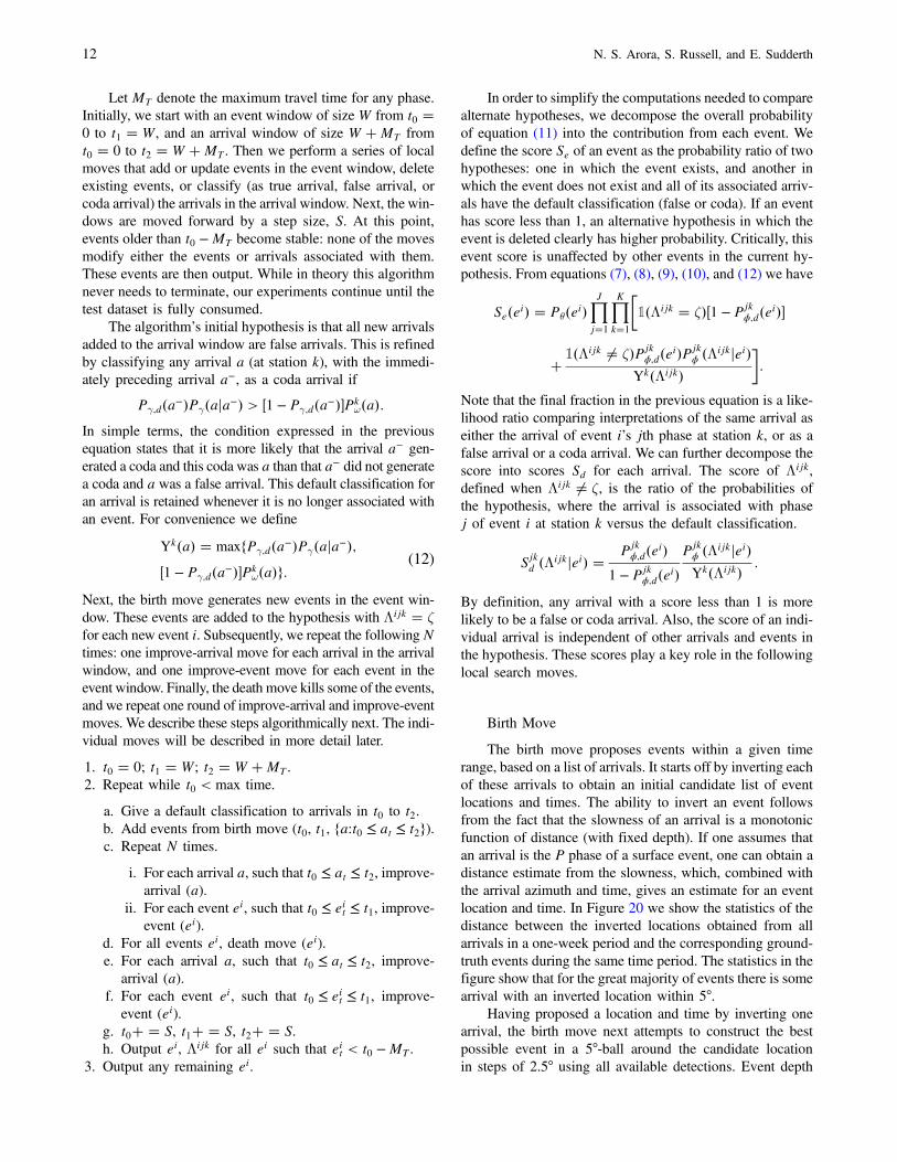
The birth move proposes events within a given timerange, based on a list of arrivals. It starts off by inverting eachof these arrivals to obtain an initial candidate list of eventlocations and times. The ability to invert an event followsfrom the fact that the slowness of an arrival is a monotonicfunction of distance (with fixed depth). If one assumes thatan arrival is the P phase of a surface event, one can obtain adistance estimate from the slowness, which, combined withthe arrival azimuth and time, gives an estimate for an eventlocation and time. In Figure 20 we show the statistics of thedistance between the inverted locations obtained from allarrivals in a one-week period and the corresponding ground-truth events during the same time period. The statistics in thefigure show that for the great majority of events there is somearrival with an inverted location within 5°.

Having proposed a location and time by inverting onearrival, the birth move next attempts to construct the bestpossible event in a 5°-ball around the candidate locationin steps of 2.5° using all available detections. Event depth


is fixed to the surface, and two possible magnitude values areused (3 and 4). The event time is computed from the IASPEImodel using the current event location and the arrival time.The best such event is further optimized using the improve-arrival and improve-event moves and then set aside. Thisprocess is repeated as long as the best event has a scoregreater than 1. An event is not allowed to use arrivals asso-ciated with events found earlier in this process. Finally, allthe events generated in this process are returned (withouttheir associated arrivals). In algorithmic form, the processis as follows:

1. Given t0, t1, and arrivals A.2. Repeat for each a in A.

a. Invert a to obtain a candidate location ιa.b. Repeat for each location e in a ball around ιa.

i. Initialize Λe.ii. Repeat for each arrival a in A (let k be a’s station).

A. Determine the phase j with the maximumscore Sjkd �aje�.

B. If Sjkd �aje� > Sjkd �Λjkje� or if Λjk � ζ andSjkd �aje� > 1, then set Λjk � a.

3. Let e be the event with the maximum score Se�e� instep 2.

4. Repeat 100 times.

a. Invoke improve-event �e�.b. Invoke improve-arrival (a) for all a in A with e as the

only potential event.5. If Se�e� > 1, then set aside event e, and remove arrivals

in Λejk from A, then go to step 2.6. Return set-aside events.

Note that the design of the birth move allows for easyparallelization using threads. On a machine with multipleCPU cores, a simple variant of the previously described birth

move is employed. In step 2, the arrivals are divided equallyamong the threads. Each thread uses its arrivals to compute itscandidate events that are then evaluated against all the arrivalsto compute the best event. Finally, in step 3 the overall bestevent from among all the threads is computed in serial.

Improve-Arrival Move

For each arrival in the arrival window, we consider allpossible phases j of all events i up to MT seconds earlier.We then associate the best event–phase pair for this arrivalthat is not already assigned to an arrival with higher scoreat the same station k. If this best event–phase pair has scoreSjkd �Λijkjei� < 1, the arrival is changed to its default status(one of false or coda). In more precise terms:

1. Given arrival a at station k.2. Repeat for each event e.

a. Determine the phase j with the maximum scoreSjkd �Λejkje�.

3. Let e be the event with the maximum score Sjkd �Λejkje�.4. If Sjkd �aje� > Sjkd �Λejkje� or if Λejk � ζ and Sjkd �aje� >

1, then set Λejk � a.

Improve-Event Move

For each event ei, we consider 100 points chosen uni-formly at random in a small ball around the event (2° in lon-gitude and latitude, 100 km in depth, 5 s in time, and 2 unitsof magnitude), and choose those attributes with the highestscore Se�ei�.

Death Move

Any event ei with score Se�ei� < 1 is deleted, and all ofits currently associated arrivals are marked as false alarms.

(a) (b)

Figure 20. Distance between events and inverted locations within 10° and 100 s. (a) The figure shows the distance from a true event andthe nearest inverted location. (b) The figure shows the converse, that is, the distance from an inverted location to the nearest true event. Thecolor version of this figure is available only in the electronic edition.


Note that the birth move is not a greedy move: the pro-posed event will almost always have a score Se�ei� < 1 untilsome number of arrivals are assigned in subsequent moves.The overall structure of these moves could be easily con-verted to a Markov chain Monte-Carlo (MCMC) method or

simulated annealing algorithm. However, in our experimentsthis search outperformed simple MCMC methods in terms ofspeed and accuracy.

Experimental Results

Metrics

We compute the accuracy of an event history hypothesisby comparison to a chosen ground-truth history. A bipartitegraph is created between predicted and true events. An edgeis added between a predicted and a true event that is at most5° in distance and 50 s in time apart. The weight of the edge isthe distance between the two events. Finally, a minimumweight–maximum cardinality matching is computed on thegraph. We report three quantities from this matching, preci-sion (percentage of predicted events that are matched), recall(percentage of true events that are matched), and average er-ror (average distance in kilometers between matched events).

Summary of Results

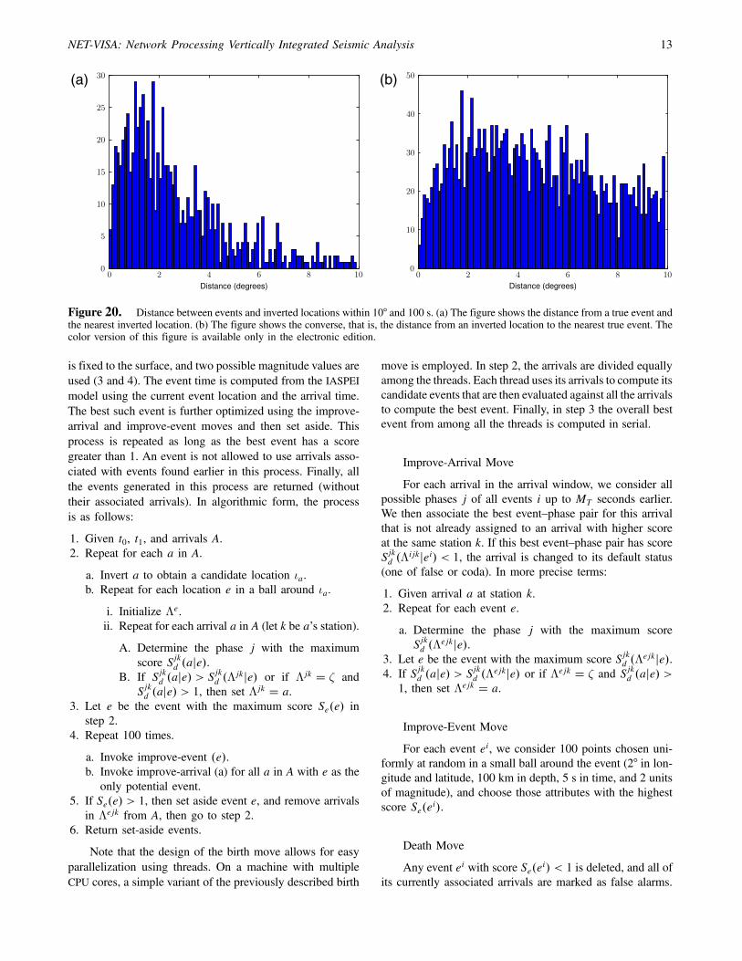
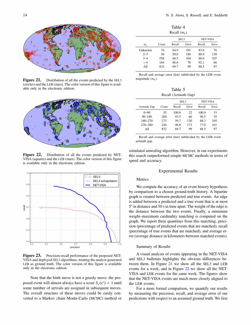
A visual analysis of events appearing in the NET-VISAand SEL3 bulletins highlights the obvious differences be-tween them. In Figure 21 we show all the SEL3 and LEBevents for a week, and in Figure 22 we show all the NET-VISA and LEB events for the same week. The figures showthat the NET-VISA events are much more closely aligned tothe LEB events.

For a more formal comparison, we quantify our resultsby measuring the precision, recall, and average error of ourpredictions with respect to an assumed ground truth. We first

Figure 21. Distribution of all the events predicted by the SEL3(circles) and the LEB (stars). The color version of this figure is avail-able only in the electronic edition.

Figure 22. Distribution of all the events predicted by NET-VISA (squares) and the LEB (stars). The color version of this figureis available only in the electronic edition.

Figure 23. Precision-recall performance of the proposed NET-VISA and deployed SEL3 algorithms, treating the analyst-generatedLEB as ground truth. The color version of this figure is availableonly in the electronic edition.

Table 4Recall (mb)

SEL3 NET-VISA

mb Count Recall Error Recall Error

Unknown 74 64.9 101 83.8 762–3 36 50.0 186 88.9 1303–4 558 66.5 104 88.0 107>4 164 86.6 70 92.1 66All 832 69.7 99 88.5 97

Recall and average error (km) subdivided by the LEB eventmagnitude (mb).

Table 5Recall (Azimuth Gap)

SEL3 NET-VISA

Azimuth Gap Count Recall Error Recall Error

0–90 55 100.0 22 100.0 3390–180 260 93.5 66 96.5 55180–270 273 59.7 120 88.3 105270–360 244 48.8 173 77.0 161

All 832 69.7 99 88.5 97

Recall and average error (km) subdivided by the LEB eventazimuth gap.


treat the IDC analyst-generated LEB as the ground truth, andcompare the performance of our NET-VISA algorithm to thecurrently deployed GA system and the SEL3 bulletin it pro-duces. Because there is a natural trade-off between precisionand recall, for example, perfect recall can be achieved at theexpense of precision by reporting events in all locations at alltimes, it is common in statistics and machine learning tocompute a precision–recall curve showing the best recall thatcan be achieved for each possible level of precision (or viceversa). In NET-VISA, the curve is generated by adjusting thescore threshold for including events in the bulletin: a higherthreshold increases precision but lowers recall (see Fig. 23).Because we are not able to adjust the GA software, we havemarked SEL3 on the graph as a single point. NET-VISA hasat least 18% more recall at the same precision as the SEL3,and at least 38% more precision at the same recall as theSEL3. Put another way, NET-VISA reduces the number ofmissed events by about 60%.

Also in this figure, we show an extrapolated precision–recall curve for the SEL3 using scores from a Support VectorMachine trained to classify true and false SEL3 events fromthe work of Mackey et al. (2009). Next, we discuss furtherthe right (high-precision) end of this curve.

For completeness, we note the following run-time statis-tics: The NET-VISA inference algorithm used a window size,W, of 30minutes; a step size, S, of 15 minutes; andN � 1000

iterations. The inference for 1weekof data took about 4.5 dayson a single CPU core running at 2.5 GHz. Estimating modelparameters from2.5months of training data took about 1 hour.

The arrivals include those from both the primary andauxiliary stations in the IMS network. Although both theNET-VISA bulletin and the SEL3 were produced using thesame set of arrivals, the GA algorithm treats arrivals fromauxiliary IMS stations differently. These arrivals are not al-

lowed to drive event formation. NET-VISA makes no suchdistinction, and thus enjoys a slight advantage.

Underconstrained Events

To further understand why NET-VISA is able to findevents missed by the SEL3, we subdivide the NET-VISA andthe SEL3 recall and average error by two different criteria. InTable 4 we subdivide by the LEB event magnitude. For mag-nitudes up to 4, NET-VISA has nearly 20% higher recall withsimilar error. In Table 5 we subdivide by the LEB eventazimuth gap. The azimuth gap of an event is the largest differ-ence between successive event-to-station azimuths for sta-tions where the automated processing detected an arrival forthe event. Large gaps indicate that the event location is under-constrained. For example, if all stations are to the southwest ofan event, the gap is greater than 270°, and the event will bepoorly localized along a line running from southwest to north-east. The results in these two tables highlight a commontheme: NET-VISA performs significantly better than the SEL3whenever there are less data available. Under these circum-stances the additional information in the NET-VISA model,location prior, amplitude, nondetections, etc., plays a criticalrole in determining a better location for the events.

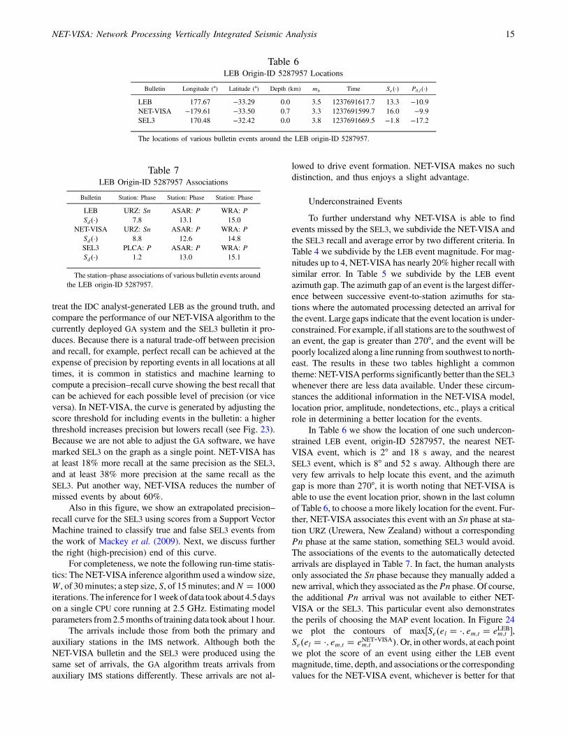
In Table 6 we show the location of one such undercon-strained LEB event, origin-ID 5287957, the nearest NET-VISA event, which is 2° and 18 s away, and the nearestSEL3 event, which is 8° and 52 s away. Although there arevery few arrivals to help locate this event, and the azimuthgap is more than 270°, it is worth noting that NET-VISA isable to use the event location prior, shown in the last columnof Table 6, to choose a more likely location for the event. Fur-ther, NET-VISA associates this event with an Sn phase at sta-tion URZ (Urewera, New Zealand) without a correspondingPn phase at the same station, something SEL3 would avoid.The associations of the events to the automatically detectedarrivals are displayed in Table 7. In fact, the human analystsonly associated the Sn phase because they manually added anew arrival, which they associated as thePn phase. Of course,the additional Pn arrival was not available to either NET-VISA or the SEL3. This particular event also demonstratesthe perils of choosing the MAP event location. In Figure 24we plot the contours of max�Se�el � ·; em;t � eLEBm;t �,Se�el � ·; em;t � eNET-VISAm;t �. Or, in other words, at each pointwe plot the score of an event using either the LEB eventmagnitude, time, depth, and associations or the correspondingvalues for the NET-VISA event, whichever is better for that

Table 6LEB Origin-ID 5287957 Locations

Bulletin Longitude (°) Latitude (°) Depth (km) mb Time Se�·� Pθ;l�·�LEB 177.67 −33.29 0.0 3.5 1237691617.7 13.3 −10.9NET-VISA −179:61 −33.50 0.7 3.3 1237691599.7 16.0 −9.9SEL3 170.48 −32.42 0.0 3.8 1237691669.5 −1:8 −17.2

The locations of various bulletin events around the LEB origin-ID 5287957.

Table 7LEB Origin-ID 5287957 Associations

Bulletin Station: Phase Station: Phase Station: Phase

LEB URZ: Sn ASAR: P WRA: PSd�·� 7.8 13.1 15.0

NET-VISA URZ: Sn ASAR: P WRA: PSd�·� 8.8 12.6 14.8SEL3 PLCA: P ASAR: P WRA: PSd�·� 1.2 13.0 15.1

The station–phase associations of various bulletin events aroundthe LEB origin-ID 5287957.


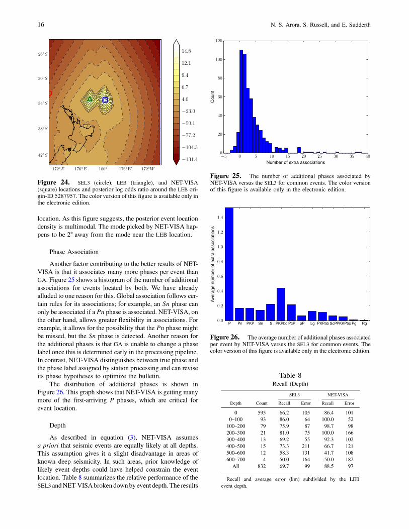
location. As this figure suggests, the posterior event locationdensity is multimodal. The mode picked by NET-VISA hap-pens to be 2° away from the mode near the LEB location.

Phase Association

Another factor contributing to the better results of NET-VISA is that it associates many more phases per event thanGA. Figure 25 shows a histogram of the number of additionalassociations for events located by both. We have alreadyalluded to one reason for this. Global association follows cer-tain rules for its associations; for example, an Sn phase canonly be associated if a Pn phase is associated. NET-VISA, onthe other hand, allows greater flexibility in associations. Forexample, it allows for the possibility that the Pn phase mightbe missed, but the Sn phase is detected. Another reason forthe additional phases is that GA is unable to change a phaselabel once this is determined early in the processing pipeline.In contrast, NET-VISA distinguishes between true phase andthe phase label assigned by station processing and can reviseits phase hypotheses to optimize the bulletin.

The distribution of additional phases is shown inFigure 26. This graph shows that NET-VISA is getting manymore of the first-arriving P phases, which are critical forevent location.

Depth

As described in equation (3), NET-VISA assumesa priori that seismic events are equally likely at all depths.This assumption gives it a slight disadvantage in areas ofknown deep seismicity. In such areas, prior knowledge oflikely event depths could have helped constrain the eventlocation. Table 8 summarizes the relative performance of theSEL3 andNET-VISAbroken downby event depth. The results

Figure 24. SEL3 (circle), LEB (triangle), and NET-VISA(square) locations and posterior log odds ratio around the LEB ori-gin-ID 5287957. The color version of this figure is available only inthe electronic edition.

Figure 25. The number of additional phases associated byNET-VISA versus the SEL3 for common events. The color versionof this figure is available only in the electronic edition.

Figure 26. The average number of additional phases associatedper event by NET-VISA versus the SEL3 for common events. Thecolor version of this figure is available only in the electronic edition.

Table 8Recall (Depth)

SEL3 NET-VISA

Depth Count Recall Error Recall Error

0 595 66.2 105 86.4 1010–100 93 86.0 64 100.0 52100–200 79 75.9 87 98.7 98200–300 21 81.0 75 100.0 166300–400 13 69.2 55 92.3 102400–500 15 73.3 211 66.7 121500–600 12 58.3 131 41.7 108600–700 4 50.0 164 50.0 182

All 832 69.7 99 88.5 97

Recall and average error (km) subdivided by the LEBevent depth.


in the table suggest that NET-VISA has slightly poorer resultsfor events at depth more than 400 km, although there are toofew deep events in this dataset to support a definite finding.

Comparison with Regional Bulletins

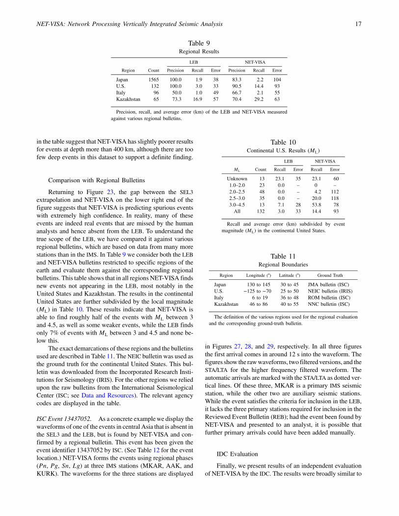
Returning to Figure 23, the gap between the SEL3extrapolation and NET-VISA on the lower right end of thefigure suggests that NET-VISA is predicting spurious eventswith extremely high confidence. In reality, many of theseevents are indeed real events that are missed by the humananalysts and hence absent from the LEB. To understand thetrue scope of the LEB, we have compared it against variousregional bulletins, which are based on data from many morestations than in the IMS. In Table 9 we consider both the LEBand NET-VISA bulletins restricted to specific regions of theearth and evaluate them against the corresponding regionalbulletins. This table shows that in all regions NET-VISA findsnew events not appearing in the LEB, most notably in theUnited States and Kazakhstan. The results in the continentalUnited States are further subdivided by the local magnitude(ML) in Table 10. These results indicate that NET-VISA isable to find roughly half of the events with ML between 3and 4.5, as well as some weaker events, while the LEB findsonly 7% of events with ML between 3 and 4.5 and none be-low this.

The exact demarcations of these regions and the bulletinsused are described in Table 11. The NEIC bulletin was used asthe ground truth for the continental United States. This bul-letin was downloaded from the Incorporated Research Insti-tutions for Seismology (IRIS). For the other regions we reliedupon the raw bulletins from the International SeismologicalCenter (ISC; see Data and Resources). The relevant agencycodes are displayed in the table.

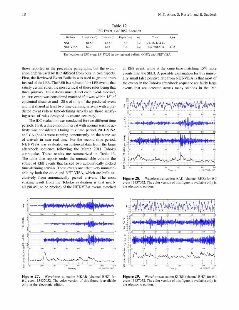
ISC Event 13437052. As a concrete examplewe display thewaveforms of one of the events in central Asia that is absent inthe SEL3 and the LEB, but is found by NET-VISA and con-firmed by a regional bulletin. This event has been given theevent identifier 13437052 by ISC. (See Table 12 for the eventlocation.) NET-VISA forms the events using regional phases(Pn, Pg, Sn, Lg) at three IMS stations (MKAR, AAK, andKURK). The waveforms for the three stations are displayed

in Figures 27, 28, and 29, respectively. In all three figuresthe first arrival comes in around 12 s into the waveform. Thefigures show the rawwaveforms, two filtered versions, and theSTA/LTA for the higher frequency filtered waveform. Theautomatic arrivals are marked with the STA/LTA as dotted ver-tical lines. Of these three, MKAR is a primary IMS seismicstation, while the other two are auxiliary seismic stations.While the event satisfies the criteria for inclusion in the LEB,it lacks the three primary stations required for inclusion in theReviewed Event Bulletin (REB); had the event been found byNET-VISA and presented to an analyst, it is possible thatfurther primary arrivals could have been added manually.

IDC Evaluation

Finally, we present results of an independent evaluationof NET-VISA by the IDC. The results were broadly similar to

Table 9Regional Results

LEB NET-VISA

Region Count Precision Recall Error Precision Recall Error

Japan 1565 100.0 1.9 38 83.3 2.2 104U.S. 132 100.0 3.0 33 90.5 14.4 93Italy 96 50.0 1.0 49 66.7 2.1 55Kazakhstan 65 73.3 16.9 57 70.4 29.2 63

Precision, recall, and average error (km) of the LEB and NET-VISA measuredagainst various regional bulletins.

Table 10Continental U.S. Results (ML)

LEB NET-VISA

ML Count Recall Error Recall Error

Unknown 13 23.1 35 23.1 601.0–2.0 23 0.0 – 0 –2.0–2.5 48 0.0 – 4.2 1122.5–3.0 35 0.0 – 20.0 1183.0–4.5 13 7.1 28 53.8 78All 132 3.0 33 14.4 93

Recall and average error (km) subdivided by eventmagnitude (ML) in the continental United States.

Table 11Regional Boundaries

Region Longitude (°) Latitude (°) Ground Truth

Japan 130 to 145 30 to 45 JMA bulletin (ISC)U.S. −125 to −70 25 to 50 NEIC bulletin (IRIS)Italy 6 to 19 36 to 48 ROM bulletin (ISC)Kazakhstan 46 to 86 40 to 55 NNC bulletin (ISC)

The definition of the various regions used for the regional evaluationand the corresponding ground-truth bulletin.


those reported in the preceding paragraphs, but the evalu-ation criteria used by IDC differed from ours in two aspects.First, the Reviewed Event Bulletin was used as ground truthinstead of the LEB. The REB is a subset of the LEB events thatsatisfy certain rules, the most critical of these rules being thatthree primary IMS stations must detect each event. Second,an REB event was considered matched if it was within 18° ofepicentral distance and 120 s of time of the predicted eventand if it shared at least two time-defining arrivals with a pre-dicted event (where time-defining arrivals are those satisfy-ing a set of rules designed to ensure accuracy).

The IDC evaluation was conducted for two different timeperiods. First, a three-month interval with normal seismic ac-tivity was considered. During this time period, NET-VISAand GA (SEL3) were running concurrently on the same setof arrivals in near real time. For the second time period,NET-VISA was evaluated on historical data from the largeaftershock sequence following the March 2011 Tohokuearthquake. These results are summarized in Table 13.The table also reports under the unmatchable column thesubset of REB events that lacked two automatically pickedtime-defining arrivals. These events are effectively unmatch-able by both the SEL3 and NET-VISA, which are built ex-clusively from automatically picked arrivals. The moststriking result from the Tohoku evaluation is that nearlyall (98.4%, to be precise) of the NET-VISA events matched

an REB event, while at the same time matching 15% moreevents than the SEL3. A possible explanation for this unusu-ally small false positive rate from NET-VISA is that most ofthe events in the Tohoku aftershock sequence are fairly largeevents that are detected across many stations in the IMS

Table 12ISC Event 13437052 Location

Bulletin Longitude (°) Latitude (°) Depth (km) mb Time Se�·�NNC 81.53 42.37 3.9 3.2 1237760634.43NET-VISA 82.7 42.5 0.4 2.2 1237760637.8 47.2

The location of ISC event 13437052 in the regional bulletin (NNC) and NET-VISA.

Figure 27. Waveforms at station MKAR (channel BHZ) forISC event 13437052. The color version of this figure is availableonly in the electronic edition.

Figure 28. Waveforms at station AAK (channel BHZ) for ISCevent 13437052. The color version of this figure is available only inthe electronic edition.

Figure 29. Waveforms at station KURK (channel BHZ) for ISCevent 13437052. The color version of this figure is available only inthe electronic edition.


network, and in particular many primary stations, thussatisfying the criteria for REB inclusion.

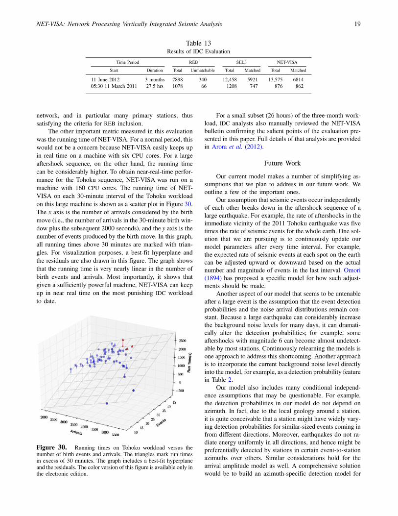
The other important metric measured in this evaluationwas the running time of NET-VISA. For a normal period, thiswould not be a concern because NET-VISA easily keeps upin real time on a machine with six CPU cores. For a largeaftershock sequence, on the other hand, the running timecan be considerably higher. To obtain near-real-time perfor-mance for the Tohoku sequence, NET-VISA was run on amachine with 160 CPU cores. The running time of NET-VISA on each 30-minute interval of the Tohoku workloadon this large machine is shown as a scatter plot in Figure 30.The x axis is the number of arrivals considered by the birthmove (i.e., the number of arrivals in the 30-minute birth win-dow plus the subsequent 2000 seconds), and the y axis is thenumber of events produced by the birth move. In this graph,all running times above 30 minutes are marked with trian-gles. For visualization purposes, a best-fit hyperplane andthe residuals are also drawn in this figure. The graph showsthat the running time is very nearly linear in the number ofbirth events and arrivals. Most importantly, it shows thatgiven a sufficiently powerful machine, NET-VISA can keepup in near real time on the most punishing IDC workloadto date.

For a small subset (26 hours) of the three-month work-load, IDC analysts also manually reviewed the NET-VISAbulletin confirming the salient points of the evaluation pre-sented in this paper. Full details of that analysis are providedin Arora et al. (2012).

Future Work

Our current model makes a number of simplifying as-sumptions that we plan to address in our future work. Weoutline a few of the important ones.

Our assumption that seismic events occur independentlyof each other breaks down in the aftershock sequence of alarge earthquake. For example, the rate of aftershocks in theimmediate vicinity of the 2011 Tohoku earthquake was fivetimes the rate of seismic events for the whole earth. One sol-ution that we are pursuing is to continuously update ourmodel parameters after every time interval. For example,the expected rate of seismic events at each spot on the earthcan be adjusted upward or downward based on the actualnumber and magnitude of events in the last interval. Omori(1894) has proposed a specific model for how such adjust-ments should be made.

Another aspect of our model that seems to be untenableafter a large event is the assumption that the event detectionprobabilities and the noise arrival distributions remain con-stant. Because a large earthquake can considerably increasethe background noise levels for many days, it can dramati-cally alter the detection probabilities; for example, someaftershocks with magnitude 6 can become almost undetect-able by most stations. Continuously relearning the models isone approach to address this shortcoming. Another approachis to incorporate the current background noise level directlyinto the model, for example, as a detection probability featurein Table 2.

Our model also includes many conditional independ-ence assumptions that may be questionable. For example,the detection probabilities in our model do not depend onazimuth. In fact, due to the local geology around a station,it is quite conceivable that a station might have widely vary-ing detection probabilities for similar-sized events coming infrom different directions. Moreover, earthquakes do not ra-diate energy uniformly in all directions, and hence might bepreferentially detected by stations in certain event-to-stationazimuths over others. Similar considerations hold for thearrival amplitude model as well. A comprehensive solutionwould be to build an azimuth-specific detection model for

Table 13Results of IDC Evaluation

Time Period REB SEL3 NET-VISA

Start Duration Total Unmatchable Total Matched Total Matched

11 June 2012 3 months 7898 340 12,458 5921 13,575 681405:30 11 March 2011 27.5 hrs 1078 66 1208 747 876 862

Figure 30. Running times on Tohoku workload versus thenumber of birth events and arrivals. The triangles mark run timesin excess of 30 minutes. The graph includes a best-fit hyperplaneand the residuals. The color version of this figure is available only inthe electronic edition.


each station and to add the moment tensor as an event attrib-ute in the model. The energy radiation pattern for a seismicevent is clearly very important for the CTBTO because itcould be used as a discriminant for explosions and earth-quakes. The radiation pattern can also account for the corre-lations between the detection probabilities of nearby stations,as well as the correlations between different phases at thesame station.

Elaborating the model by adding dependencies and newhidden variables (such as the moment tensor) is certainlyfeasible, but may require additional historical data to estimatethe necessary parameters. Whether such steps improve mon-itoring performance remains to be seen. As noted in theIntroduction, we are also extending the generative modeldownward to include waveform characteristics. In this way,detection becomes part of a globally integrated inferenceprocess and hence susceptible to top-down influences, ratherthan being a purely local, bottom-up, hard-threshold decision.

Conclusions

Our results demonstrate that a Bayesian approach to seis-mic monitoring can improve significantly on the performanceof classical systems. The NET-VISA system cannot onlyreduce the human analyst effort required to achieve a givenlevel of accuracy, but it can also lower the magnitude thresh-old for reliable detection. Given that the difficulty of seismicmonitoring was cited as one of the principal reasons for non-ratification of the CTBT by the United States Senate in 1999,one hopes that improvements in monitoring may increase thechances of final ratification and entry into force.

Putting monitoring onto a sound probabilistic footingalso facilitates further improvements such as continuous es-timation of local noise conditions, travel time, and attenuationmodels without the need for ground-truth calibration experi-ments (controlled explosions). Moreover, it facilitates anopen-source approach, whereby various expert groups can de-vise and test more refined and accurate model componentsand contribute them as modules in an open probabilisticarchitecture.

Data and Resources

A three-month dataset of IMS arrivals, covering theperiod 22 March to 20 June 2009, was made available bythe CTBTO through the Virtual Data Exploitation Center,or vDEC (Vaidya et al., 2009). All of the results described hereexcept for the IDC evaluation were produced using seven daysof data from the validation set (22 March to 29March). Therewere a total of 832 LEB events during this period and roughly120,000 arrivals. The training set was 2.5 months (5 April to20 June), including 8313 LEB events and 1,163,848 arrivals.

Additional data were obtained for regional bulletin com-parisons from IRIS at http://www.iris.edu/SeismiQuery/sq‑events.htm (last accessed January 2012) and from ISC athttp://www.isc.ac.uk/iscbulletin/search/catalogue/ (last ac-

cessed July 2011). International Seismological Center isavailable at http://www.isc.ac.uk (last accessed July 2011).

Acknowledgments

We would like to thank the many seismologists who patientlyexplained to us the intricacies of their field, among them Ronan LeBras,Robert Engdahl, David Bowers, Bob Pearce, Stephen Myers, DmitryStorchak, Istvan Bondar, and Barbara Romanowicz. Paul Kidwell of theLawrence Livermore National Laboratory designed the features for the eventdetection probability and wrote the initial parameter estimation code for thecorresponding weights. We also received assistance from several Berkeleyundergraduates, including Matthew Cann, Hong Hu, Christopher Lin,Andrew Lee, Tony Dear, and Ron Sun.

We are grateful to Alexander Poplavskiy for providing the results ofthe IDC evaluation. The specific evaluation criteria was devised by DmitryBobrov.

All the results in this paper except for the IDC evaluation were obtainedon the Amazon EC2 cluster, which was made possible by an AWS in Edu-cation grant award.

The facilities of the IRIS Data Management System, and specificallythe IRIS Data Management Center, were used for access to waveform andmetadata required in this study. The IRIS DMS is funded through the NationalScience Foundation and specifically the GEO Directorate through the Instru-mentation and Facilities Program of the National Science Foundation underCooperative Agreement EAR-0552316.

All the authors were partially supported by the Preparatory Commis-sion for the CTBT.

References

Allen, R. (1978). Automatic earthquake recognition and timing from singletraces, Bull. Seismol. Soc. Am. 68, 1521–1532.

Arora, N. S., J. Given, E. Tomuta, S. Russell, and S. Spiliopoulos (2012).Analyst evaluation of model-based Bayesian seismic monitoring atthe CTBTO, in The 34th Monitoring Research Review: Ground-BasedNuclear Explosion Monitoring Technologies, Albuquerque, NewMexico.

Bar-Shalom, Y., and T. Fortmann (1988). Tracking and Data Association,Academic Press, Orlando, Florida.

Cormen, T. H., C. E. Leiserson, R. L. Rivest, and C. Stein (2009). Introduc-tion to Algorithms, Third Ed., MIT Press and McGraw-Hill, Cam-bridge, Massachusetts.

Duijndam, A. J. W. (1988a). Bayesian-estimation in seismic inversion. Part2. Uncertainty Analysis, Geophys. Prospect. 36, no. 8, 899.

Duijndam, A. J. W. (1988b). Bayesian estimation in seismic inversion. Part I:Principles, Geophys. Prospect. 36, no. 8, 878–898.

Geiger, L. (1910). Herdbestimmung bei erdbeden ans den ankunftzeiten,K. Gessel. Wiss. Goett. 4, 331–349 (in German).

Geiger, L. (1912). Probability method for the determination ofearthquake epicenters from the arrival time only, Bull. St. Louis Univ.8, 60–71.

Gelman, A., J. B. Carlin, H. S. Stern, and D. B. Rubin (2004). Bayesian DataAnalysis, Chapman & Hall, Boca Raton, Florida.

Gutenberg, B., and C. Richter (1954). Seismicity of the Earth and AssociatedPhenomena, Second Ed., Princeton University Press, Princeton,New Jersey.

Lay, T., and T. C. Wallace (1995). Modern Global Seismology, AcademicPress, San Diego, California.

Le Bras, R., H. Swanger, T. Sereno, G. Beall, and R. Jenkins (1994). Globalassociation, Science Applications International Corp. Tech. Rept.ADA304805, San Diego, California.

Mackey, L., A. Kleiner, and M. I. Jordan (2009). Improved automatedseismic event extraction using machine learning (abstract S31B-1714), Eos Trans. AGU 90, no. 52, Fall Meet. Suppl.


http://www.iris.edu/SeismiQuery/sq-events.htm





http://www.isc.ac.uk/iscbulletin/search/catalogue/

http://www.isc.ac.uk

Magotra, N., N. Ahmed, and E. Chael (1987). Seismic event detectionand source location using single-station (three-component) data, Bull.Seismol. Soc. Am. 77, 958–971.

Menke, W. (1989). Geophysical Data Analysis: Discrete Inverse Theory,Academic Press, San Diego, California.

Myers, S. C., G. Johannesson, and W. Hanley (2007). A Bayesian hierar-chical method for multiple-event seismic location, Geophys. J. Int.171, 1049–1063.

Omori, F. (1894). On the aftershocks of earthquakes, Journal of the Collegeof Science, Imperial University of Tokyo 7, 111–200.

Roberts, R. G., A. Christoffersson, and F. Cassidy (1989). Real-timeevent detection, phase identification and source location estimationusing single station three-component seismic data, Geophys. J. 97,471–480.

Storchak, D. A., J. Schweitzer, and P. Bormann (2003). The IASPEIstandard seismic phase list, Seismol. Res. Lett. 74, no. 6, 761–772.

Vaidya, S., R. Engdahl, R. Le Bras, K. Koch, and O. Dahlman (2009).Strategic initiative in support of CTBT data processing: vDEC (virtualData Exploitation Centre) (abstract DM-01/A), in CTBTOInternational Scientific Studies, Hofburg, Vienna, Austria, 10–12 June2009.

Waldhauser, F., and W. L. Ellsworth (2000). A double-difference earthquakelocation algorithm: Method and application to the northern Haywardfault, California, Bull. Seismol. Soc. Am. 90, 1353–1368.

Bayesian Logic, Inc.32432 Lighthouse WayUnion City, California [email protected]

(N.S.A.)

Computer Science Division,387 Soda HallUniversity of CaliforniaBerkeley, California [email protected]

(S.R.)

Department of Computer ScienceBrown University115 Waterman Street, Box 1910Providence, Rhode Island [email protected]

(E.S.)

Manuscript received 26 March 2012


Documents

NET-VISA: Network Processing Vertically …russell/papers/bssa-netvisa.pdfNET-VISA: Network Processing Vertically Integrated Seismic Analysis ... A Bayesian seismic monitoring system,