Embed Size (px)
Citation preview
Neural Networks:Optimization & Regularization
Shan-Hung [email protected]
Department of Computer Science,National Tsing Hua University, Taiwan
Machine Learning
Shan-Hung Wu (CS, NTHU) NN Opt & Reg Machine Learning 1 / 60
Outline
1 OptimizationMomentum & Nesterov MomentumAdaGrad & RMSPropBatch NormalizationContinuation Methods & Curriculum Learning
2 RegularizationWeight DecayData AugmentationDropoutManifold RegularizationDomain-Specific Model Design
Shan-Hung Wu (CS, NTHU) NN Opt & Reg Machine Learning 2 / 60
Outline
1 OptimizationMomentum & Nesterov MomentumAdaGrad & RMSPropBatch NormalizationContinuation Methods & Curriculum Learning
2 RegularizationWeight DecayData AugmentationDropoutManifold RegularizationDomain-Specific Model Design
Shan-Hung Wu (CS, NTHU) NN Opt & Reg Machine Learning 3 / 60
Challenges
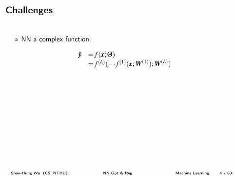
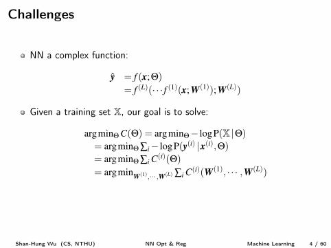
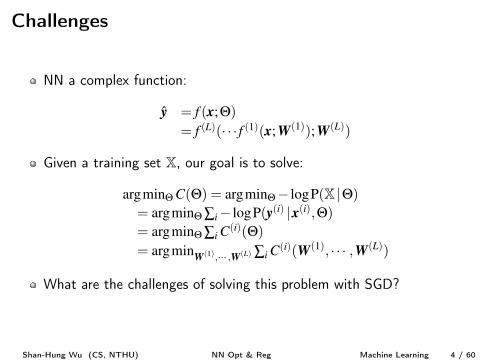
NN a complex function:
ˆy = f (x;Q)= f
(L)(· · · f (1)(x;W
(1));W
(L))
Given a training set X, our goal is to solve:
argminQ C(Q) = argminQ� logP(X |Q)= argminQ Â
i
� logP(y(i) |x(i),Q)= argminQ Â
i
C
(i)(Q)= argmin
W
(1),··· ,W(L) Âi
C
(i)(W(1), · · · ,W(L))
What are the challenges of solving this problem with SGD?
Shan-Hung Wu (CS, NTHU) NN Opt & Reg Machine Learning 4 / 60
Challenges
NN a complex function:
ˆy = f (x;Q)= f
(L)(· · · f (1)(x;W
(1));W
(L))
Given a training set X, our goal is to solve:
argminQ C(Q) = argminQ� logP(X |Q)= argminQ Â
i
� logP(y(i) |x(i),Q)= argminQ Â
i
C
(i)(Q)= argmin
W
(1),··· ,W(L) Âi
C
(i)(W(1), · · · ,W(L))
What are the challenges of solving this problem with SGD?
Shan-Hung Wu (CS, NTHU) NN Opt & Reg Machine Learning 4 / 60
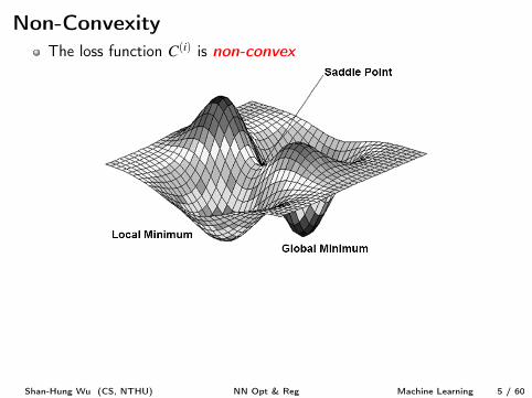
Non-ConvexityThe loss function C
(i) is non-convex
SGD stops at local minima or saddle pointsPrior to the success of SGD (in roughly 2012), NN cost functionsurfaces were generally believed to have many non-convex structureHowever, studies [2, 4] show SGD seldom encounters critical pointswhen training a large NN
Shan-Hung Wu (CS, NTHU) NN Opt & Reg Machine Learning 5 / 60
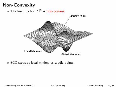
Non-ConvexityThe loss function C
(i) is non-convex
SGD stops at local minima or saddle points
Prior to the success of SGD (in roughly 2012), NN cost functionsurfaces were generally believed to have many non-convex structureHowever, studies [2, 4] show SGD seldom encounters critical pointswhen training a large NN
Shan-Hung Wu (CS, NTHU) NN Opt & Reg Machine Learning 5 / 60
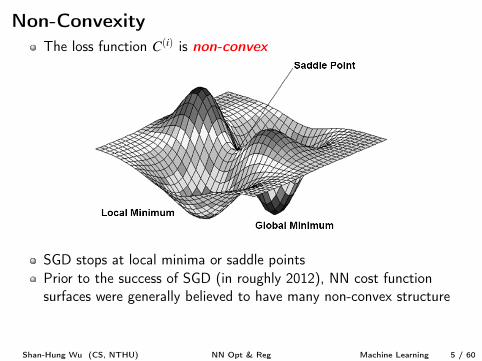
Non-ConvexityThe loss function C
(i) is non-convex
SGD stops at local minima or saddle pointsPrior to the success of SGD (in roughly 2012), NN cost functionsurfaces were generally believed to have many non-convex structure
However, studies [2, 4] show SGD seldom encounters critical pointswhen training a large NN
Shan-Hung Wu (CS, NTHU) NN Opt & Reg Machine Learning 5 / 60
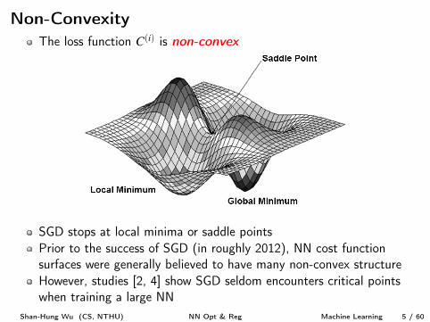
Non-ConvexityThe loss function C
(i) is non-convex
SGD stops at local minima or saddle pointsPrior to the success of SGD (in roughly 2012), NN cost functionsurfaces were generally believed to have many non-convex structureHowever, studies [2, 4] show SGD seldom encounters critical pointswhen training a large NN
Shan-Hung Wu (CS, NTHU) NN Opt & Reg Machine Learning 5 / 60
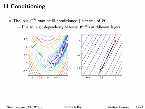
Ill-Conditioning
The loss C
(i) may be ill-conditioned (in terms of Q)Due to, e.g., dependency between W
(k)’s at different layers
SGD has slow progress at valleys or plateaus
Shan-Hung Wu (CS, NTHU) NN Opt & Reg Machine Learning 6 / 60
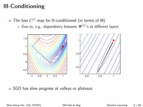
Ill-Conditioning
The loss C
(i) may be ill-conditioned (in terms of Q)Due to, e.g., dependency between W
(k)’s at different layers
SGD has slow progress at valleys or plateaus
Shan-Hung Wu (CS, NTHU) NN Opt & Reg Machine Learning 6 / 60
Lacks Global Minima
The loss C
(i) may lack a global minimum point
E.g., for multiclass classificationP(y |x,Q) provided by a softmax functionC
(i)(Q) =� logP(y(i) |x(i),Q) can become arbitrarily close to zero (ifclassifying example i correctly)But not actually reaching zero
SGD may proceed along adirection foreverInitialization is important
Shan-Hung Wu (CS, NTHU) NN Opt & Reg Machine Learning 7 / 60
Lacks Global Minima
The loss C
(i) may lack a global minimum pointE.g., for multiclass classification
P(y |x,Q) provided by a softmax function
C
(i)(Q) =� logP(y(i) |x(i),Q) can become arbitrarily close to zero (ifclassifying example i correctly)But not actually reaching zero
SGD may proceed along adirection foreverInitialization is important
Shan-Hung Wu (CS, NTHU) NN Opt & Reg Machine Learning 7 / 60
Lacks Global Minima
The loss C
(i) may lack a global minimum pointE.g., for multiclass classification
P(y |x,Q) provided by a softmax functionC
(i)(Q) =� logP(y(i) |x(i),Q) can become arbitrarily close to zero (ifclassifying example i correctly)
But not actually reaching zero
SGD may proceed along adirection foreverInitialization is important
Shan-Hung Wu (CS, NTHU) NN Opt & Reg Machine Learning 7 / 60
Lacks Global Minima
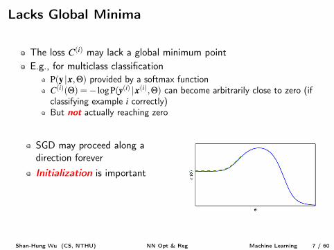
The loss C
(i) may lack a global minimum pointE.g., for multiclass classification
P(y |x,Q) provided by a softmax functionC
(i)(Q) =� logP(y(i) |x(i),Q) can become arbitrarily close to zero (ifclassifying example i correctly)But not actually reaching zero
SGD may proceed along adirection foreverInitialization is important
Shan-Hung Wu (CS, NTHU) NN Opt & Reg Machine Learning 7 / 60
Lacks Global Minima
The loss C
(i) may lack a global minimum pointE.g., for multiclass classification
P(y |x,Q) provided by a softmax functionC
(i)(Q) =� logP(y(i) |x(i),Q) can become arbitrarily close to zero (ifclassifying example i correctly)But not actually reaching zero
SGD may proceed along adirection foreverInitialization is important
Shan-Hung Wu (CS, NTHU) NN Opt & Reg Machine Learning 7 / 60
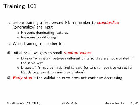
Training 101
Before training a feedforward NN, remember to standardize
(z-normalize) the input
Prevents dominating featuresImproves conditioning
When training, remember to:
1 Initialize all weights to small random values
Breaks “symmetry” between different units so they are not updated inthe same wayBiases b
(k)’s may be initialized to zero (or to small positive values forReLUs to prevent too much saturation)
2Early stop if the validation error does not continue decreasing
Prevents overfitting
Shan-Hung Wu (CS, NTHU) NN Opt & Reg Machine Learning 8 / 60
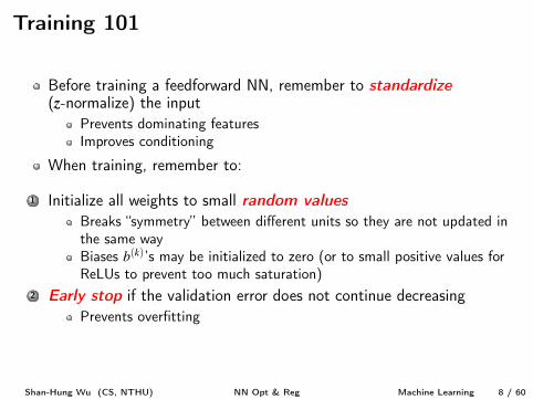
Training 101
Before training a feedforward NN, remember to standardize
(z-normalize) the inputPrevents dominating featuresImproves conditioning
When training, remember to:
1 Initialize all weights to small random values
Breaks “symmetry” between different units so they are not updated inthe same wayBiases b
(k)’s may be initialized to zero (or to small positive values forReLUs to prevent too much saturation)
2Early stop if the validation error does not continue decreasing
Prevents overfitting
Shan-Hung Wu (CS, NTHU) NN Opt & Reg Machine Learning 8 / 60
Training 101
Before training a feedforward NN, remember to standardize
(z-normalize) the inputPrevents dominating featuresImproves conditioning
When training, remember to:
1 Initialize all weights to small random values
Breaks “symmetry” between different units so they are not updated inthe same way
Biases b
(k)’s may be initialized to zero (or to small positive values forReLUs to prevent too much saturation)
2Early stop if the validation error does not continue decreasing
Prevents overfitting
Shan-Hung Wu (CS, NTHU) NN Opt & Reg Machine Learning 8 / 60
Training 101
Before training a feedforward NN, remember to standardize
(z-normalize) the inputPrevents dominating featuresImproves conditioning
When training, remember to:
1 Initialize all weights to small random values
Breaks “symmetry” between different units so they are not updated inthe same wayBiases b
(k)’s may be initialized to zero
(or to small positive values forReLUs to prevent too much saturation)
2Early stop if the validation error does not continue decreasing
Prevents overfitting
Shan-Hung Wu (CS, NTHU) NN Opt & Reg Machine Learning 8 / 60
Training 101
Before training a feedforward NN, remember to standardize
(z-normalize) the inputPrevents dominating featuresImproves conditioning
When training, remember to:
1 Initialize all weights to small random values
Breaks “symmetry” between different units so they are not updated inthe same wayBiases b
(k)’s may be initialized to zero (or to small positive values forReLUs to prevent too much saturation)
2Early stop if the validation error does not continue decreasing
Prevents overfitting
Shan-Hung Wu (CS, NTHU) NN Opt & Reg Machine Learning 8 / 60
Training 101
Before training a feedforward NN, remember to standardize
(z-normalize) the inputPrevents dominating featuresImproves conditioning
When training, remember to:
1 Initialize all weights to small random values
Breaks “symmetry” between different units so they are not updated inthe same wayBiases b
(k)’s may be initialized to zero (or to small positive values forReLUs to prevent too much saturation)
2Early stop if the validation error does not continue decreasing
Prevents overfitting
Shan-Hung Wu (CS, NTHU) NN Opt & Reg Machine Learning 8 / 60
Outline
1 OptimizationMomentum & Nesterov MomentumAdaGrad & RMSPropBatch NormalizationContinuation Methods & Curriculum Learning
2 RegularizationWeight DecayData AugmentationDropoutManifold RegularizationDomain-Specific Model Design
Shan-Hung Wu (CS, NTHU) NN Opt & Reg Machine Learning 9 / 60
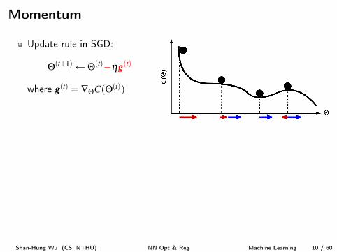
Momentum
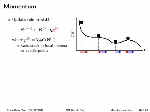
Update rule in SGD:
Q(t+1) Q(t)�hg
(t)
where g
(t) = —QC(Q(t))
Gets stuck in local minimaor saddle points
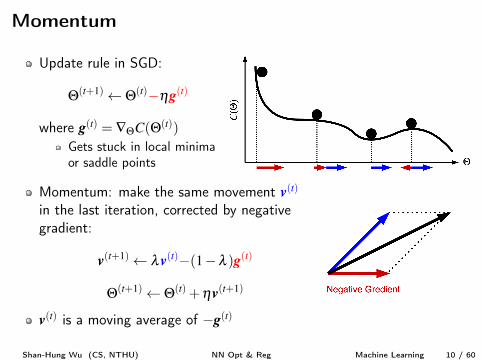
Momentum: make the same movement v
(t)
in the last iteration, corrected by negativegradient:
v
(t+1) lv
(t)�(1�l )g(t)
Q(t+1) Q(t) +hv
(t+1)
v
(t) is a moving average of �g
(t)
Shan-Hung Wu (CS, NTHU) NN Opt & Reg Machine Learning 10 / 60
Momentum
Update rule in SGD:
Q(t+1) Q(t)�hg
(t)
where g
(t) = —QC(Q(t))Gets stuck in local minimaor saddle points
Momentum: make the same movement v
(t)
in the last iteration, corrected by negativegradient:
v
(t+1) lv
(t)�(1�l )g(t)
Q(t+1) Q(t) +hv
(t+1)
v
(t) is a moving average of �g
(t)
Shan-Hung Wu (CS, NTHU) NN Opt & Reg Machine Learning 10 / 60
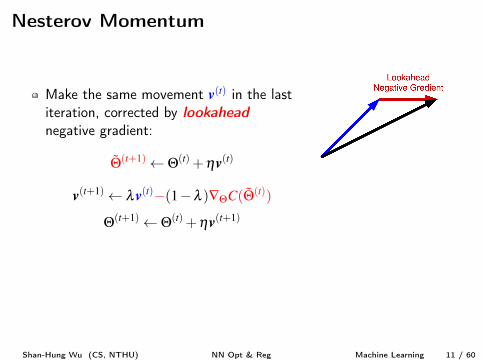
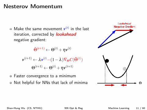
Nesterov Momentum
Make the same movement v
(t) in the lastiteration, corrected by lookahead
negative gradient:
˜Q(t+1) Q(t) +hv
(t)
v
(t+1) lv
(t)�(1�l )—QC( ˜Q(t))
Q(t+1) Q(t) +hv
(t+1)
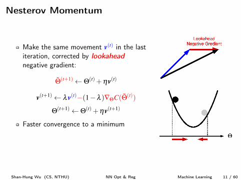
Faster convergence to a minimumNot helpful for NNs that lack of minima
Shan-Hung Wu (CS, NTHU) NN Opt & Reg Machine Learning 11 / 60
Nesterov Momentum
Make the same movement v
(t) in the lastiteration, corrected by lookahead
negative gradient:
˜Q(t+1) Q(t) +hv
(t)
v
(t+1) lv
(t)�(1�l )—QC( ˜Q(t))
Q(t+1) Q(t) +hv
(t+1)
Faster convergence to a minimum
Not helpful for NNs that lack of minima
Shan-Hung Wu (CS, NTHU) NN Opt & Reg Machine Learning 11 / 60
Nesterov Momentum
Make the same movement v
(t) in the lastiteration, corrected by lookahead
negative gradient:
˜Q(t+1) Q(t) +hv
(t)
v
(t+1) lv
(t)�(1�l )—QC( ˜Q(t))
Q(t+1) Q(t) +hv
(t+1)
Faster convergence to a minimumNot helpful for NNs that lack of minima
Shan-Hung Wu (CS, NTHU) NN Opt & Reg Machine Learning 11 / 60
Outline
1 OptimizationMomentum & Nesterov MomentumAdaGrad & RMSPropBatch NormalizationContinuation Methods & Curriculum Learning
2 RegularizationWeight DecayData AugmentationDropoutManifold RegularizationDomain-Specific Model Design
Shan-Hung Wu (CS, NTHU) NN Opt & Reg Machine Learning 12 / 60
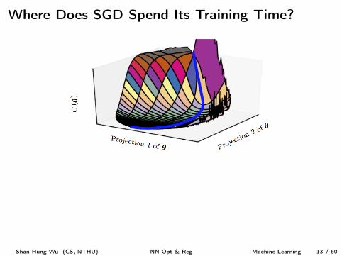
Where Does SGD Spend Its Training Time?
1 Detouring a saddle point of high costBetter initialization
2 Traversing the relatively flat valleyAdaptive learning rate
Shan-Hung Wu (CS, NTHU) NN Opt & Reg Machine Learning 13 / 60
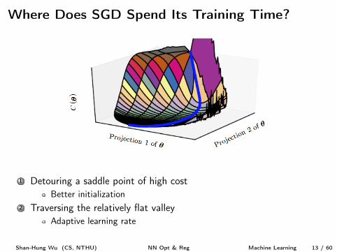
Where Does SGD Spend Its Training Time?
1 Detouring a saddle point of high costBetter initialization
2 Traversing the relatively flat valleyAdaptive learning rate
Shan-Hung Wu (CS, NTHU) NN Opt & Reg Machine Learning 13 / 60
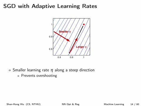
SGD with Adaptive Learning Rates
Smaller learning rate h along a steep directionPrevents overshooting
Larger learning rate h along a flat directionSpeed up convergence
How?
Shan-Hung Wu (CS, NTHU) NN Opt & Reg Machine Learning 14 / 60
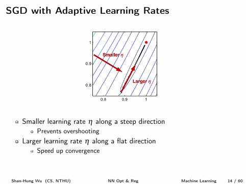
SGD with Adaptive Learning Rates
Smaller learning rate h along a steep directionPrevents overshooting
Larger learning rate h along a flat directionSpeed up convergence
How?
Shan-Hung Wu (CS, NTHU) NN Opt & Reg Machine Learning 14 / 60
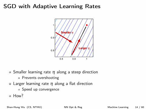
SGD with Adaptive Learning Rates
Smaller learning rate h along a steep directionPrevents overshooting
Larger learning rate h along a flat directionSpeed up convergence
How?
Shan-Hung Wu (CS, NTHU) NN Opt & Reg Machine Learning 14 / 60
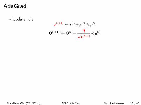
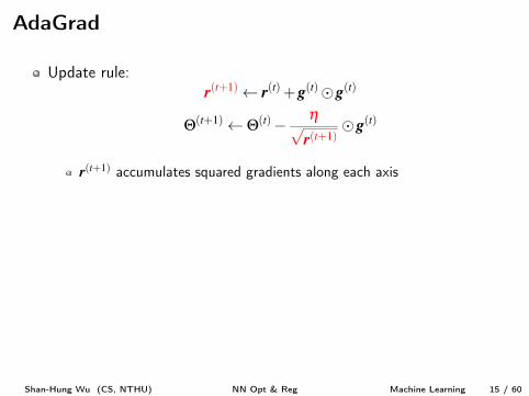
AdaGrad
Update rule:r
(t+1) r
(t) +g
(t)�g
(t)
Q(t+1) Q(t)� hpr
(t+1)�g
(t)
r
(t+1) accumulates squared gradients along each axisDivision and square root applied to r
(t+1) elementwisely
We have
hpr
(t+1)=
hpt+1
� 1q1
t+1
r
(t+1)=
hpt+1
� 1q1
t+1
Ât
i=0
g
(i)�g
(i)
1Smaller learning rate along all directions as t grows
2Larger learning rate along more gently sloped directions
Shan-Hung Wu (CS, NTHU) NN Opt & Reg Machine Learning 15 / 60
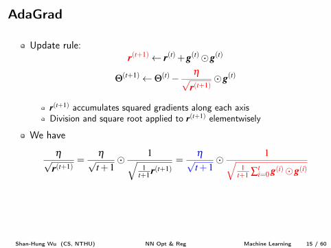
AdaGrad
Update rule:r
(t+1) r
(t) +g
(t)�g
(t)
Q(t+1) Q(t)� hpr
(t+1)�g
(t)
r
(t+1) accumulates squared gradients along each axis
Division and square root applied to r
(t+1) elementwisely
We have
hpr
(t+1)=
hpt+1
� 1q1
t+1
r
(t+1)=
hpt+1
� 1q1
t+1
Ât
i=0
g
(i)�g
(i)
1Smaller learning rate along all directions as t grows
2Larger learning rate along more gently sloped directions
Shan-Hung Wu (CS, NTHU) NN Opt & Reg Machine Learning 15 / 60
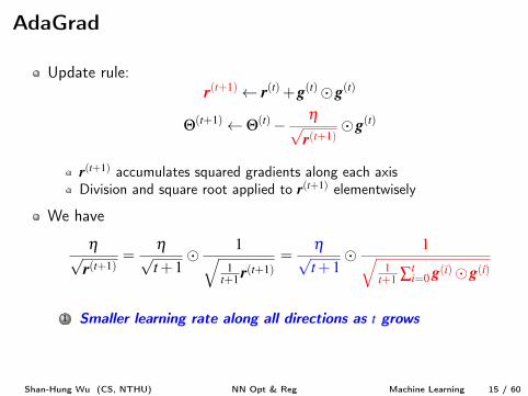
AdaGrad
Update rule:r
(t+1) r
(t) +g
(t)�g
(t)
Q(t+1) Q(t)� hpr
(t+1)�g
(t)
r
(t+1) accumulates squared gradients along each axisDivision and square root applied to r
(t+1) elementwisely
We have
hpr
(t+1)=
hpt+1
� 1q1
t+1
r
(t+1)=
hpt+1
� 1q1
t+1
Ât
i=0
g
(i)�g
(i)
1Smaller learning rate along all directions as t grows
2Larger learning rate along more gently sloped directions
Shan-Hung Wu (CS, NTHU) NN Opt & Reg Machine Learning 15 / 60
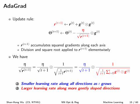
AdaGrad
Update rule:r
(t+1) r
(t) +g
(t)�g
(t)
Q(t+1) Q(t)� hpr
(t+1)�g
(t)
r
(t+1) accumulates squared gradients along each axisDivision and square root applied to r
(t+1) elementwisely
We have
hpr
(t+1)=
hpt+1
� 1q1
t+1
r
(t+1)=
hpt+1
� 1q1
t+1
Ât
i=0
g
(i)�g
(i)
1Smaller learning rate along all directions as t grows
2Larger learning rate along more gently sloped directions
Shan-Hung Wu (CS, NTHU) NN Opt & Reg Machine Learning 15 / 60
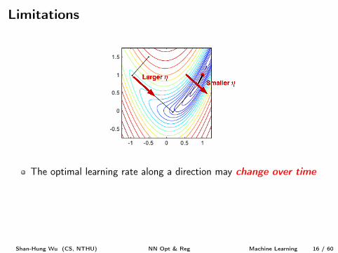
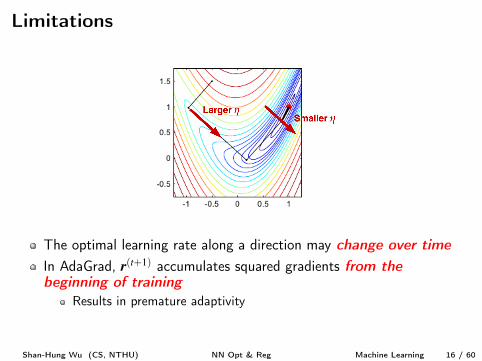
Limitations
The optimal learning rate along a direction may change over time
In AdaGrad, r
(t+1) accumulates squared gradients from the
beginning of training
Results in premature adaptivity
Shan-Hung Wu (CS, NTHU) NN Opt & Reg Machine Learning 16 / 60
Limitations
The optimal learning rate along a direction may change over time
In AdaGrad, r
(t+1) accumulates squared gradients from the
beginning of training
Results in premature adaptivity
Shan-Hung Wu (CS, NTHU) NN Opt & Reg Machine Learning 16 / 60
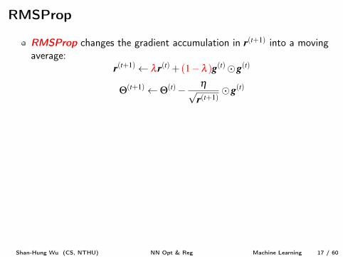
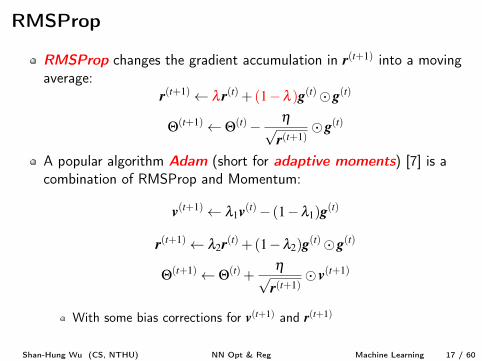
RMSProp
RMSProp changes the gradient accumulation in r
(t+1) into a movingaverage:
r
(t+1) l r
(t) + (1�l )g(t)�g
(t)
Q(t+1) Q(t)� hpr
(t+1)�g
(t)
A popular algorithm Adam (short for adaptive moments) [7] is acombination of RMSProp and Momentum:
v
(t+1) l1
v
(t)� (1�l1
)g(t)
r
(t+1) l2
r
(t) + (1�l2
)g(t)�g
(t)
Q(t+1) Q(t) +hp
r
(t+1)� v
(t+1)
With some bias corrections for v
(t+1) and r
(t+1)
Shan-Hung Wu (CS, NTHU) NN Opt & Reg Machine Learning 17 / 60

Outline
1 OptimizationMomentum & Nesterov MomentumAdaGrad & RMSPropBatch NormalizationContinuation Methods & Curriculum Learning
2 RegularizationWeight DecayData AugmentationDropoutManifold RegularizationDomain-Specific Model Design
Shan-Hung Wu (CS, NTHU) NN Opt & Reg Machine Learning 18 / 60
Training Deep NNs I
So far, we modify the optimization algorithm to better train the model
Can we modify the model to ease the optimization task?What are the difficulties in training a deep NN?
Shan-Hung Wu (CS, NTHU) NN Opt & Reg Machine Learning 19 / 60
Training Deep NNs I
So far, we modify the optimization algorithm to better train the modelCan we modify the model to ease the optimization task?
What are the difficulties in training a deep NN?
Shan-Hung Wu (CS, NTHU) NN Opt & Reg Machine Learning 19 / 60
Training Deep NNs I
So far, we modify the optimization algorithm to better train the modelCan we modify the model to ease the optimization task?What are the difficulties in training a deep NN?
Shan-Hung Wu (CS, NTHU) NN Opt & Reg Machine Learning 19 / 60
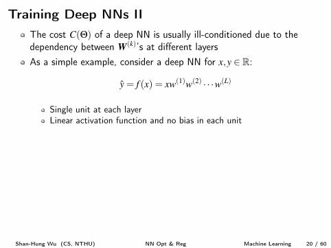
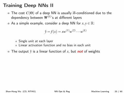
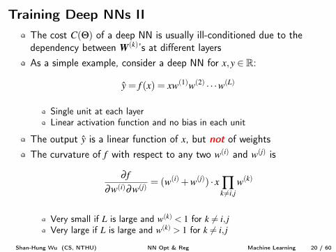
Training Deep NNs IIThe cost C(Q) of a deep NN is usually ill-conditioned due to thedependency between W
(k)’s at different layers
As a simple example, consider a deep NN for x,y 2 R:
y = f (x) = xw
(1)w
(2) · · ·w(L)
Single unit at each layerLinear activation function and no bias in each unit
The output y is a linear function of x, but not of weightsThe curvature of f with respect to any two w
(i) and w
(j) is
∂ f
∂w
(i)∂w
(j)= (w(i) +w
(j)) · x ’k 6=i,j
w
(k)
Very small if L is large and w
(k) < 1 for k 6= i, jVery large if L is large and w
(k) > 1 for k 6= i, j
Shan-Hung Wu (CS, NTHU) NN Opt & Reg Machine Learning 20 / 60
Training Deep NNs IIThe cost C(Q) of a deep NN is usually ill-conditioned due to thedependency between W
(k)’s at different layersAs a simple example, consider a deep NN for x,y 2 R:
y = f (x) = xw
(1)w
(2) · · ·w(L)
Single unit at each layerLinear activation function and no bias in each unit
The output y is a linear function of x, but not of weights
The curvature of f with respect to any two w
(i) and w
(j) is
∂ f
∂w
(i)∂w
(j)= (w(i) +w
(j)) · x ’k 6=i,j
w
(k)
Very small if L is large and w
(k) < 1 for k 6= i, jVery large if L is large and w
(k) > 1 for k 6= i, j
Shan-Hung Wu (CS, NTHU) NN Opt & Reg Machine Learning 20 / 60
Training Deep NNs IIThe cost C(Q) of a deep NN is usually ill-conditioned due to thedependency between W
(k)’s at different layersAs a simple example, consider a deep NN for x,y 2 R:
y = f (x) = xw
(1)w
(2) · · ·w(L)
Single unit at each layerLinear activation function and no bias in each unit
The output y is a linear function of x, but not of weightsThe curvature of f with respect to any two w
(i) and w
(j) is
∂ f
∂w
(i)∂w
(j)= (w(i) +w
(j)) · x ’k 6=i,j
w
(k)
Very small if L is large and w
(k) < 1 for k 6= i, jVery large if L is large and w
(k) > 1 for k 6= i, j
Shan-Hung Wu (CS, NTHU) NN Opt & Reg Machine Learning 20 / 60
Training Deep NNs IIIThe ill-conditioned C(Q) makes a gradient-based optimizationalgorithm (e.g., SGD) inefficient
Let Q = [w(1),w(2), · · · ,w(L)]> and g
(t) = —QC(Q(t))
In gradient descent, we get Q(t+1) by Q(t+1) Q(t)�hg
(t) based onthe first-order Taylor approximation of C
The gradient g
(t)i
= ∂C
∂w
(i) (Q(t)) is calculated individually by fixingC(Q(t)) in other dimensions (w(j)’s, j 6= i)However, g
(t) updates Q(t) in all dimensions simultaneously in thesame iterationC(Q(t+1)) will be guaranteed to decrease only if C is linear at Q(t)
Wrong assumption: Q(t+1)i
will decrease C even if other Q(t+1)j
’s areupdated simultaneouslySecond-order methods?
Time consumingDoes not take into account high-order effects
Can we change the model to make this assumption not-so-wrong?
Shan-Hung Wu (CS, NTHU) NN Opt & Reg Machine Learning 21 / 60
Training Deep NNs IIIThe ill-conditioned C(Q) makes a gradient-based optimizationalgorithm (e.g., SGD) inefficientLet Q = [w(1),w(2), · · · ,w(L)]> and g
(t) = —QC(Q(t))
In gradient descent, we get Q(t+1) by Q(t+1) Q(t)�hg
(t) based onthe first-order Taylor approximation of C
The gradient g
(t)i
= ∂C
∂w
(i) (Q(t)) is calculated individually by fixingC(Q(t)) in other dimensions (w(j)’s, j 6= i)
However, g
(t) updates Q(t) in all dimensions simultaneously in thesame iterationC(Q(t+1)) will be guaranteed to decrease only if C is linear at Q(t)
Wrong assumption: Q(t+1)i
will decrease C even if other Q(t+1)j
’s areupdated simultaneouslySecond-order methods?
Time consumingDoes not take into account high-order effects
Can we change the model to make this assumption not-so-wrong?
Shan-Hung Wu (CS, NTHU) NN Opt & Reg Machine Learning 21 / 60
Training Deep NNs IIIThe ill-conditioned C(Q) makes a gradient-based optimizationalgorithm (e.g., SGD) inefficientLet Q = [w(1),w(2), · · · ,w(L)]> and g
(t) = —QC(Q(t))
In gradient descent, we get Q(t+1) by Q(t+1) Q(t)�hg
(t) based onthe first-order Taylor approximation of C
The gradient g
(t)i
= ∂C
∂w
(i) (Q(t)) is calculated individually by fixingC(Q(t)) in other dimensions (w(j)’s, j 6= i)However, g
(t) updates Q(t) in all dimensions simultaneously in thesame iteration
C(Q(t+1)) will be guaranteed to decrease only if C is linear at Q(t)
Wrong assumption: Q(t+1)i
will decrease C even if other Q(t+1)j
’s areupdated simultaneouslySecond-order methods?
Time consumingDoes not take into account high-order effects
Can we change the model to make this assumption not-so-wrong?
Shan-Hung Wu (CS, NTHU) NN Opt & Reg Machine Learning 21 / 60
Training Deep NNs IIIThe ill-conditioned C(Q) makes a gradient-based optimizationalgorithm (e.g., SGD) inefficientLet Q = [w(1),w(2), · · · ,w(L)]> and g
(t) = —QC(Q(t))
In gradient descent, we get Q(t+1) by Q(t+1) Q(t)�hg
(t) based onthe first-order Taylor approximation of C
The gradient g
(t)i
= ∂C
∂w
(i) (Q(t)) is calculated individually by fixingC(Q(t)) in other dimensions (w(j)’s, j 6= i)However, g
(t) updates Q(t) in all dimensions simultaneously in thesame iterationC(Q(t+1)) will be guaranteed to decrease only if C is linear at Q(t)
Wrong assumption: Q(t+1)i
will decrease C even if other Q(t+1)j
’s areupdated simultaneouslySecond-order methods?
Time consumingDoes not take into account high-order effects
Can we change the model to make this assumption not-so-wrong?
Shan-Hung Wu (CS, NTHU) NN Opt & Reg Machine Learning 21 / 60
Training Deep NNs IIIThe ill-conditioned C(Q) makes a gradient-based optimizationalgorithm (e.g., SGD) inefficientLet Q = [w(1),w(2), · · · ,w(L)]> and g
(t) = —QC(Q(t))
In gradient descent, we get Q(t+1) by Q(t+1) Q(t)�hg
(t) based onthe first-order Taylor approximation of C
The gradient g
(t)i
= ∂C
∂w
(i) (Q(t)) is calculated individually by fixingC(Q(t)) in other dimensions (w(j)’s, j 6= i)However, g
(t) updates Q(t) in all dimensions simultaneously in thesame iterationC(Q(t+1)) will be guaranteed to decrease only if C is linear at Q(t)
Wrong assumption: Q(t+1)i
will decrease C even if other Q(t+1)j
’s areupdated simultaneously
Second-order methods?Time consumingDoes not take into account high-order effects
Can we change the model to make this assumption not-so-wrong?
Shan-Hung Wu (CS, NTHU) NN Opt & Reg Machine Learning 21 / 60
Training Deep NNs IIIThe ill-conditioned C(Q) makes a gradient-based optimizationalgorithm (e.g., SGD) inefficientLet Q = [w(1),w(2), · · · ,w(L)]> and g
(t) = —QC(Q(t))
In gradient descent, we get Q(t+1) by Q(t+1) Q(t)�hg
(t) based onthe first-order Taylor approximation of C
The gradient g
(t)i
= ∂C
∂w
(i) (Q(t)) is calculated individually by fixingC(Q(t)) in other dimensions (w(j)’s, j 6= i)However, g
(t) updates Q(t) in all dimensions simultaneously in thesame iterationC(Q(t+1)) will be guaranteed to decrease only if C is linear at Q(t)
Wrong assumption: Q(t+1)i
will decrease C even if other Q(t+1)j
’s areupdated simultaneouslySecond-order methods?
Time consumingDoes not take into account high-order effects
Can we change the model to make this assumption not-so-wrong?
Shan-Hung Wu (CS, NTHU) NN Opt & Reg Machine Learning 21 / 60
Training Deep NNs IIIThe ill-conditioned C(Q) makes a gradient-based optimizationalgorithm (e.g., SGD) inefficientLet Q = [w(1),w(2), · · · ,w(L)]> and g
(t) = —QC(Q(t))
In gradient descent, we get Q(t+1) by Q(t+1) Q(t)�hg
(t) based onthe first-order Taylor approximation of C
The gradient g
(t)i
= ∂C
∂w
(i) (Q(t)) is calculated individually by fixingC(Q(t)) in other dimensions (w(j)’s, j 6= i)However, g
(t) updates Q(t) in all dimensions simultaneously in thesame iterationC(Q(t+1)) will be guaranteed to decrease only if C is linear at Q(t)
Wrong assumption: Q(t+1)i
will decrease C even if other Q(t+1)j
’s areupdated simultaneouslySecond-order methods?
Time consumingDoes not take into account high-order effects
Can we change the model to make this assumption not-so-wrong?Shan-Hung Wu (CS, NTHU) NN Opt & Reg Machine Learning 21 / 60
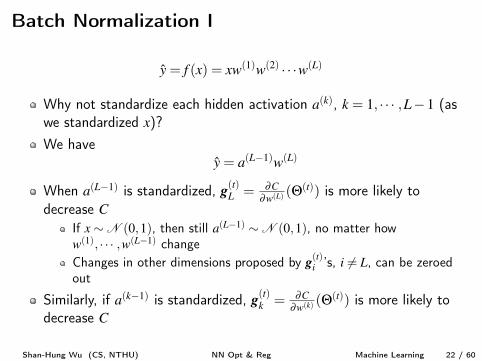
Batch Normalization I
y = f (x) = xw
(1)w
(2) · · ·w(L)
Why not standardize each hidden activation a
(k), k = 1, · · · ,L�1 (aswe standardized x)?
We havey = a
(L�1)w
(L)
When a
(L�1) is standardized, g
(t)L
= ∂C
∂w
(L) (Q(t)) is more likely todecrease C
If x⇠N (0,1), then still a
(L�1) ⇠N (0,1), no matter howw
(1), · · · ,w(L�1) changeChanges in other dimensions proposed by g
(t)i
’s, i 6= L, can be zeroedout
Similarly, if a
(k�1) is standardized, g
(t)k
= ∂C
∂w
(k) (Q(t)) is more likely todecrease C
Shan-Hung Wu (CS, NTHU) NN Opt & Reg Machine Learning 22 / 60
Batch Normalization I
y = f (x) = xw
(1)w
(2) · · ·w(L)
Why not standardize each hidden activation a
(k), k = 1, · · · ,L�1 (aswe standardized x)?We have
y = a
(L�1)w
(L)
When a
(L�1) is standardized, g
(t)L
= ∂C
∂w
(L) (Q(t)) is more likely todecrease C
If x⇠N (0,1), then still a
(L�1) ⇠N (0,1), no matter howw
(1), · · · ,w(L�1) change
Changes in other dimensions proposed by g
(t)i
’s, i 6= L, can be zeroedout
Similarly, if a
(k�1) is standardized, g
(t)k
= ∂C
∂w
(k) (Q(t)) is more likely todecrease C
Shan-Hung Wu (CS, NTHU) NN Opt & Reg Machine Learning 22 / 60
Batch Normalization I
y = f (x) = xw
(1)w
(2) · · ·w(L)
Why not standardize each hidden activation a
(k), k = 1, · · · ,L�1 (aswe standardized x)?We have
y = a
(L�1)w
(L)
When a
(L�1) is standardized, g
(t)L
= ∂C
∂w
(L) (Q(t)) is more likely todecrease C
If x⇠N (0,1), then still a
(L�1) ⇠N (0,1), no matter howw
(1), · · · ,w(L�1) changeChanges in other dimensions proposed by g
(t)i
’s, i 6= L, can be zeroedout
Similarly, if a
(k�1) is standardized, g
(t)k
= ∂C
∂w
(k) (Q(t)) is more likely todecrease C
Shan-Hung Wu (CS, NTHU) NN Opt & Reg Machine Learning 22 / 60
Batch Normalization I
y = f (x) = xw
(1)w
(2) · · ·w(L)
Why not standardize each hidden activation a
(k), k = 1, · · · ,L�1 (aswe standardized x)?We have
y = a
(L�1)w
(L)
When a
(L�1) is standardized, g
(t)L
= ∂C
∂w
(L) (Q(t)) is more likely todecrease C
If x⇠N (0,1), then still a
(L�1) ⇠N (0,1), no matter howw
(1), · · · ,w(L�1) changeChanges in other dimensions proposed by g
(t)i
’s, i 6= L, can be zeroedout
Similarly, if a
(k�1) is standardized, g
(t)k
= ∂C
∂w
(k) (Q(t)) is more likely todecrease C
Shan-Hung Wu (CS, NTHU) NN Opt & Reg Machine Learning 22 / 60
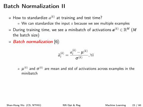
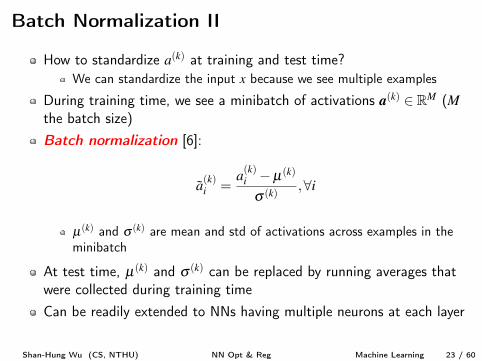
Batch Normalization II
How to standardize a
(k) at training and test time?We can standardize the input x because we see multiple examples
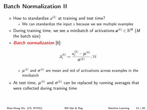
During training time, we see a minibatch of activations a
(k) 2 RM (Mthe batch size)Batch normalization [6]:
a
(k)i
=a
(k)i
�µ(k)
s (k),8i
µ(k) and s (k) are mean and std of activations across examples in theminibatch
At test time, µ(k) and s (k) can be replaced by running averages thatwere collected during training timeCan be readily extended to NNs having multiple neurons at each layer
Shan-Hung Wu (CS, NTHU) NN Opt & Reg Machine Learning 23 / 60
Batch Normalization II
How to standardize a
(k) at training and test time?We can standardize the input x because we see multiple examples
During training time, we see a minibatch of activations a
(k) 2 RM (Mthe batch size)Batch normalization [6]:
a
(k)i
=a
(k)i
�µ(k)
s (k),8i
µ(k) and s (k) are mean and std of activations across examples in theminibatch
At test time, µ(k) and s (k) can be replaced by running averages thatwere collected during training time
Can be readily extended to NNs having multiple neurons at each layer
Shan-Hung Wu (CS, NTHU) NN Opt & Reg Machine Learning 23 / 60
Batch Normalization II
How to standardize a
(k) at training and test time?We can standardize the input x because we see multiple examples
During training time, we see a minibatch of activations a
(k) 2 RM (Mthe batch size)Batch normalization [6]:
a
(k)i
=a
(k)i
�µ(k)
s (k),8i
µ(k) and s (k) are mean and std of activations across examples in theminibatch
At test time, µ(k) and s (k) can be replaced by running averages thatwere collected during training timeCan be readily extended to NNs having multiple neurons at each layer
Shan-Hung Wu (CS, NTHU) NN Opt & Reg Machine Learning 23 / 60
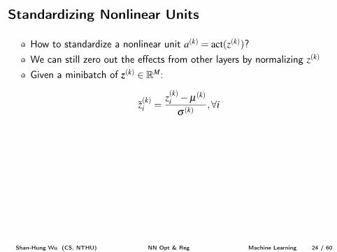
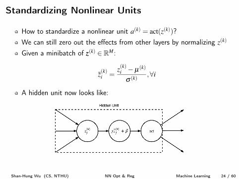
Standardizing Nonlinear Units
How to standardize a nonlinear unit a
(k) = act(z(k))?
We can still zero out the effects from other layers by normalizing z
(k)
Given a minibatch of z
(k) 2 RM:
z
(k)i
=z
(k)i
�µ(k)
s (k),8i
A hidden unit now looks like:
Shan-Hung Wu (CS, NTHU) NN Opt & Reg Machine Learning 24 / 60
Standardizing Nonlinear Units
How to standardize a nonlinear unit a
(k) = act(z(k))?We can still zero out the effects from other layers by normalizing z
(k)
Given a minibatch of z
(k) 2 RM:
z
(k)i
=z
(k)i
�µ(k)
s (k),8i
A hidden unit now looks like:
Shan-Hung Wu (CS, NTHU) NN Opt & Reg Machine Learning 24 / 60
Expressiveness I
The weights W
(k) at each layer is easier to train nowThe “wrong assumption” of gradient-based optimization is made valid
But at the cost of expressivenessNormalizing a
(k) or z
(k) limits the output range of a unitObserve that there is no need to insist a z
(k) to have zero mean andunit variance
We only care about whether it is “fixed” when calculating the gradientsfor other layers
Shan-Hung Wu (CS, NTHU) NN Opt & Reg Machine Learning 25 / 60
Expressiveness I
The weights W
(k) at each layer is easier to train nowThe “wrong assumption” of gradient-based optimization is made valid
But at the cost of expressivenessNormalizing a
(k) or z
(k) limits the output range of a unit
Observe that there is no need to insist a z
(k) to have zero mean andunit variance
We only care about whether it is “fixed” when calculating the gradientsfor other layers
Shan-Hung Wu (CS, NTHU) NN Opt & Reg Machine Learning 25 / 60
Expressiveness I
The weights W
(k) at each layer is easier to train nowThe “wrong assumption” of gradient-based optimization is made valid
But at the cost of expressivenessNormalizing a
(k) or z
(k) limits the output range of a unitObserve that there is no need to insist a z
(k) to have zero mean andunit variance
We only care about whether it is “fixed” when calculating the gradientsfor other layers
Shan-Hung Wu (CS, NTHU) NN Opt & Reg Machine Learning 25 / 60
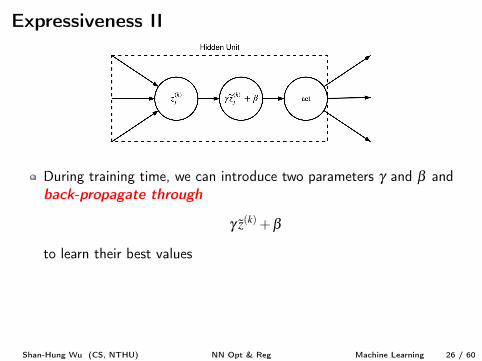
Expressiveness II
During training time, we can introduce two parameters g and b andback-propagate through
g z
(k) +b
to learn their best values
Question: g and b can be learned to invert z
(k) to get z
(k), so what’sthe point?
z
(k) = z
(k)�µ(k)
s (k) , so g z
(k) +b = s z
(k) +µ = z
(k)
The weights W
(k), g, and b are now easier to learn with SGD
Shan-Hung Wu (CS, NTHU) NN Opt & Reg Machine Learning 26 / 60
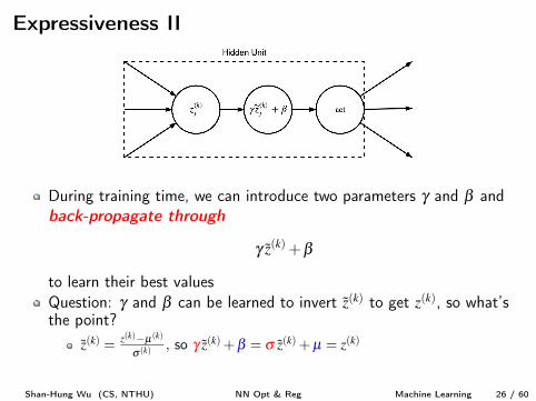
Expressiveness II
During training time, we can introduce two parameters g and b andback-propagate through
g z
(k) +b
to learn their best valuesQuestion: g and b can be learned to invert z
(k) to get z
(k), so what’sthe point?
z
(k) = z
(k)�µ(k)
s (k) , so g z
(k) +b = s z
(k) +µ = z
(k)
The weights W
(k), g, and b are now easier to learn with SGD
Shan-Hung Wu (CS, NTHU) NN Opt & Reg Machine Learning 26 / 60
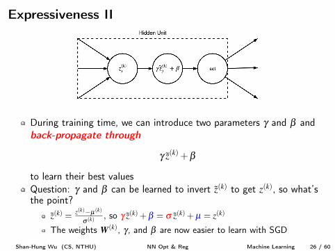
Expressiveness II
During training time, we can introduce two parameters g and b andback-propagate through
g z
(k) +b
to learn their best valuesQuestion: g and b can be learned to invert z
(k) to get z
(k), so what’sthe point?
z
(k) = z
(k)�µ(k)
s (k) , so g z
(k) +b = s z
(k) +µ = z
(k)
The weights W
(k), g, and b are now easier to learn with SGD
Shan-Hung Wu (CS, NTHU) NN Opt & Reg Machine Learning 26 / 60
Outline
1 OptimizationMomentum & Nesterov MomentumAdaGrad & RMSPropBatch NormalizationContinuation Methods & Curriculum Learning
2 RegularizationWeight DecayData AugmentationDropoutManifold RegularizationDomain-Specific Model Design
Shan-Hung Wu (CS, NTHU) NN Opt & Reg Machine Learning 27 / 60
Parameter Initialization
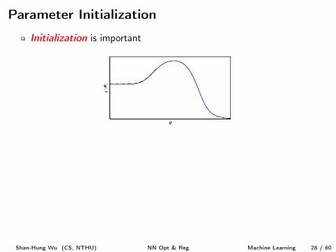
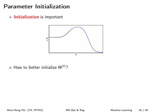
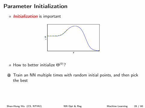
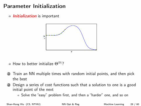
Initialization is important
How to better initialize Q(0)?
1 Train an NN multiple times with random initial points, and then pickthe best
2 Design a series of cost functions such that a solution to one is a goodinitial point of the next
Solve the “easy” problem first, and then a “harder” one, and so on
Shan-Hung Wu (CS, NTHU) NN Opt & Reg Machine Learning 28 / 60
Parameter Initialization
Initialization is important
How to better initialize Q(0)?
1 Train an NN multiple times with random initial points, and then pickthe best
2 Design a series of cost functions such that a solution to one is a goodinitial point of the next
Solve the “easy” problem first, and then a “harder” one, and so on
Shan-Hung Wu (CS, NTHU) NN Opt & Reg Machine Learning 28 / 60
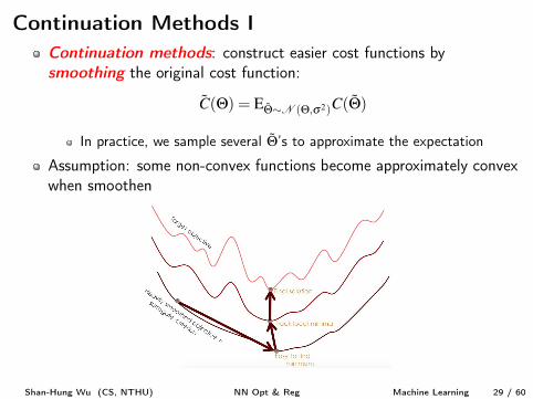
Continuation Methods IContinuation methods: construct easier cost functions bysmoothing the original cost function:
˜
C(Q) = E
˜Q⇠N (Q,s2)C( ˜Q)
In practice, we sample several ˜Q’s to approximate the expectation
Assumption: some non-convex functions become approximately convexwhen smoothen
Shan-Hung Wu (CS, NTHU) NN Opt & Reg Machine Learning 29 / 60
Continuation Methods II
Problems?
Cost function might not become convex, no matter how much it issmoothenDesigned to deal with local minima; not very helpful for NNs withoutminima
Shan-Hung Wu (CS, NTHU) NN Opt & Reg Machine Learning 30 / 60
Continuation Methods II
Problems?Cost function might not become convex, no matter how much it issmoothen
Designed to deal with local minima; not very helpful for NNs withoutminima
Shan-Hung Wu (CS, NTHU) NN Opt & Reg Machine Learning 30 / 60
Continuation Methods II
Problems?Cost function might not become convex, no matter how much it issmoothenDesigned to deal with local minima; not very helpful for NNs withoutminima
Shan-Hung Wu (CS, NTHU) NN Opt & Reg Machine Learning 30 / 60
Curriculum Learning
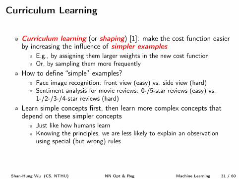
Curriculum learning (or shaping) [1]: make the cost function easierby increasing the influence of simpler examples
E.g., by assigning them larger weights in the new cost functionOr, by sampling them more frequently
How to define “simple” examples?Face image recognition: front view (easy) vs. side view (hard)Sentiment analysis for movie reviews: 0-/5-star reviews (easy) vs.1-/2-/3-/4-star reviews (hard)
Learn simple concepts first, then learn more complex concepts thatdepend on these simpler concepts
Just like how humans learnKnowing the principles, we are less likely to explain an observationusing special (but wrong) rules
Shan-Hung Wu (CS, NTHU) NN Opt & Reg Machine Learning 31 / 60
Curriculum Learning
Curriculum learning (or shaping) [1]: make the cost function easierby increasing the influence of simpler examples
E.g., by assigning them larger weights in the new cost functionOr, by sampling them more frequently
How to define “simple” examples?
Face image recognition: front view (easy) vs. side view (hard)Sentiment analysis for movie reviews: 0-/5-star reviews (easy) vs.1-/2-/3-/4-star reviews (hard)
Learn simple concepts first, then learn more complex concepts thatdepend on these simpler concepts
Just like how humans learnKnowing the principles, we are less likely to explain an observationusing special (but wrong) rules
Shan-Hung Wu (CS, NTHU) NN Opt & Reg Machine Learning 31 / 60
Curriculum Learning
Curriculum learning (or shaping) [1]: make the cost function easierby increasing the influence of simpler examples
E.g., by assigning them larger weights in the new cost functionOr, by sampling them more frequently
How to define “simple” examples?Face image recognition: front view (easy) vs. side view (hard)Sentiment analysis for movie reviews: 0-/5-star reviews (easy) vs.1-/2-/3-/4-star reviews (hard)
Learn simple concepts first, then learn more complex concepts thatdepend on these simpler concepts
Just like how humans learnKnowing the principles, we are less likely to explain an observationusing special (but wrong) rules
Shan-Hung Wu (CS, NTHU) NN Opt & Reg Machine Learning 31 / 60
Curriculum Learning
Curriculum learning (or shaping) [1]: make the cost function easierby increasing the influence of simpler examples
E.g., by assigning them larger weights in the new cost functionOr, by sampling them more frequently
How to define “simple” examples?Face image recognition: front view (easy) vs. side view (hard)Sentiment analysis for movie reviews: 0-/5-star reviews (easy) vs.1-/2-/3-/4-star reviews (hard)
Learn simple concepts first, then learn more complex concepts thatdepend on these simpler concepts
Just like how humans learnKnowing the principles, we are less likely to explain an observationusing special (but wrong) rules
Shan-Hung Wu (CS, NTHU) NN Opt & Reg Machine Learning 31 / 60
Outline
1 OptimizationMomentum & Nesterov MomentumAdaGrad & RMSPropBatch NormalizationContinuation Methods & Curriculum Learning
2 RegularizationWeight DecayData AugmentationDropoutManifold RegularizationDomain-Specific Model Design
Shan-Hung Wu (CS, NTHU) NN Opt & Reg Machine Learning 32 / 60
Regularization
The goal of an ML algorithm is to perform well not just on thetraining data, but also on new inputs
Regularization: techniques that reduce the generalization error of anML algorithm
But not the training error
By expressing preference to a simpler modelBy providing different perspectives on how to explain the training dataBy encoding prior knowledge
Shan-Hung Wu (CS, NTHU) NN Opt & Reg Machine Learning 33 / 60
Regularization
The goal of an ML algorithm is to perform well not just on thetraining data, but also on new inputsRegularization: techniques that reduce the generalization error of anML algorithm
But not the training error
By expressing preference to a simpler model
By providing different perspectives on how to explain the training dataBy encoding prior knowledge
Shan-Hung Wu (CS, NTHU) NN Opt & Reg Machine Learning 33 / 60
Regularization
The goal of an ML algorithm is to perform well not just on thetraining data, but also on new inputsRegularization: techniques that reduce the generalization error of anML algorithm
But not the training error
By expressing preference to a simpler modelBy providing different perspectives on how to explain the training data
By encoding prior knowledge
Shan-Hung Wu (CS, NTHU) NN Opt & Reg Machine Learning 33 / 60
Regularization
The goal of an ML algorithm is to perform well not just on thetraining data, but also on new inputsRegularization: techniques that reduce the generalization error of anML algorithm
But not the training error
By expressing preference to a simpler modelBy providing different perspectives on how to explain the training dataBy encoding prior knowledge
Shan-Hung Wu (CS, NTHU) NN Opt & Reg Machine Learning 33 / 60
Regularization in Deep Learning I
I have big data, do I still need to regularize my NN?The excess error is dominated by optimization error (time)
Generally, yes!For “hard” problems, the true data generating process is almostcertainly outside the model family
E.g., problems in images, audio sequences, and text domainsThe true generation process essentially involves simulating the entireuniverse
In these domains, the best fitting model (with lowest generalizationerror) is usually a larger model regularized appropriately
Shan-Hung Wu (CS, NTHU) NN Opt & Reg Machine Learning 34 / 60
Regularization in Deep Learning I
I have big data, do I still need to regularize my NN?The excess error is dominated by optimization error (time)
Generally, yes!
For “hard” problems, the true data generating process is almostcertainly outside the model family
E.g., problems in images, audio sequences, and text domainsThe true generation process essentially involves simulating the entireuniverse
In these domains, the best fitting model (with lowest generalizationerror) is usually a larger model regularized appropriately
Shan-Hung Wu (CS, NTHU) NN Opt & Reg Machine Learning 34 / 60

Regularization in Deep Learning I
I have big data, do I still need to regularize my NN?The excess error is dominated by optimization error (time)
Generally, yes!For “hard” problems, the true data generating process is almostcertainly outside the model family
E.g., problems in images, audio sequences, and text domains
The true generation process essentially involves simulating the entireuniverse
In these domains, the best fitting model (with lowest generalizationerror) is usually a larger model regularized appropriately
Shan-Hung Wu (CS, NTHU) NN Opt & Reg Machine Learning 34 / 60
Regularization in Deep Learning I
I have big data, do I still need to regularize my NN?The excess error is dominated by optimization error (time)
Generally, yes!For “hard” problems, the true data generating process is almostcertainly outside the model family
E.g., problems in images, audio sequences, and text domainsThe true generation process essentially involves simulating the entireuniverse
In these domains, the best fitting model (with lowest generalizationerror) is usually a larger model regularized appropriately
Shan-Hung Wu (CS, NTHU) NN Opt & Reg Machine Learning 34 / 60
Regularization in Deep Learning II
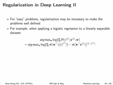
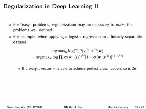
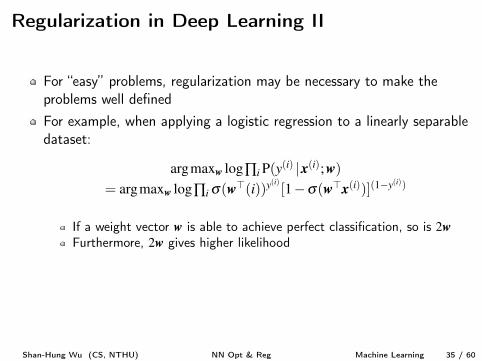
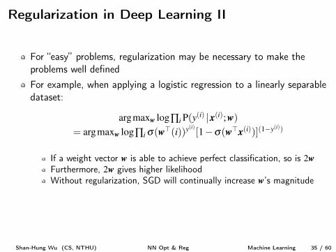
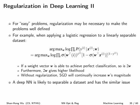
For “easy” problems, regularization may be necessary to make theproblems well defined
For example, when applying a logistic regression to a linearly separabledataset:
argmax
w
log’i
P(y(i) |x(i);w)
= argmax
w
log’i
s(w>(i))y
(i)[1�s(w>x
(i))](1�y
(i))
If a weight vector w is able to achieve perfect classification, so is 2w
Furthermore, 2w gives higher likelihoodWithout regularization, SGD will continually increase w’s magnitude
A deep NN is likely to separable a dataset and has the similar issue
Shan-Hung Wu (CS, NTHU) NN Opt & Reg Machine Learning 35 / 60
Regularization in Deep Learning II
For “easy” problems, regularization may be necessary to make theproblems well definedFor example, when applying a logistic regression to a linearly separabledataset:
argmax
w
log’i
P(y(i) |x(i);w)
= argmax
w
log’i
s(w>(i))y
(i)[1�s(w>x
(i))](1�y
(i))
If a weight vector w is able to achieve perfect classification, so is 2w
Furthermore, 2w gives higher likelihood
Without regularization, SGD will continually increase w’s magnitude
A deep NN is likely to separable a dataset and has the similar issue
Shan-Hung Wu (CS, NTHU) NN Opt & Reg Machine Learning 35 / 60
Regularization in Deep Learning II
For “easy” problems, regularization may be necessary to make theproblems well definedFor example, when applying a logistic regression to a linearly separabledataset:
argmax
w
log’i
P(y(i) |x(i);w)
= argmax
w
log’i
s(w>(i))y
(i)[1�s(w>x
(i))](1�y
(i))
If a weight vector w is able to achieve perfect classification, so is 2w
Furthermore, 2w gives higher likelihoodWithout regularization, SGD will continually increase w’s magnitude
A deep NN is likely to separable a dataset and has the similar issue
Shan-Hung Wu (CS, NTHU) NN Opt & Reg Machine Learning 35 / 60
Regularization in Deep Learning II
For “easy” problems, regularization may be necessary to make theproblems well definedFor example, when applying a logistic regression to a linearly separabledataset:
argmax
w
log’i
P(y(i) |x(i);w)
= argmax
w
log’i
s(w>(i))y
(i)[1�s(w>x
(i))](1�y
(i))
If a weight vector w is able to achieve perfect classification, so is 2w
Furthermore, 2w gives higher likelihoodWithout regularization, SGD will continually increase w’s magnitude
A deep NN is likely to separable a dataset and has the similar issue
Shan-Hung Wu (CS, NTHU) NN Opt & Reg Machine Learning 35 / 60
Outline
1 OptimizationMomentum & Nesterov MomentumAdaGrad & RMSPropBatch NormalizationContinuation Methods & Curriculum Learning
2 RegularizationWeight DecayData AugmentationDropoutManifold RegularizationDomain-Specific Model Design
Shan-Hung Wu (CS, NTHU) NN Opt & Reg Machine Learning 36 / 60

Weight Decay
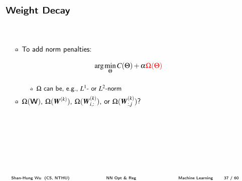
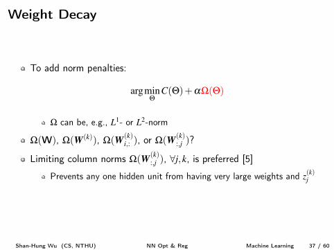
To add norm penalties:
argmin
QC(Q)+aW(Q)
W can be, e.g., L
1- or L
2-norm
W(W), W(W(k)), W(W(k)i,: ), or W(W(k)
:,j )?
Limiting column norms W(W(k):,j ), 8j,k, is preferred [5]
Prevents any one hidden unit from having very large weights and z
(k)j
Shan-Hung Wu (CS, NTHU) NN Opt & Reg Machine Learning 37 / 60
Weight Decay
To add norm penalties:
argmin
QC(Q)+aW(Q)
W can be, e.g., L
1- or L
2-norm
W(W), W(W(k)), W(W(k)i,: ), or W(W(k)
:,j )?
Limiting column norms W(W(k):,j ), 8j,k, is preferred [5]
Prevents any one hidden unit from having very large weights and z
(k)j
Shan-Hung Wu (CS, NTHU) NN Opt & Reg Machine Learning 37 / 60
Explicit Weight Decay I
Explicit norm penalties:
argmin
QC(Q) subject to W(Q) R
To solve the problem, we can use the projective SGD:At each step t, update Q(t+1) as in SGDIf Q(t+1) falls out of the feasible set, project Q(t+1) back to the tangentspace (edge) of feasible set
Advantage?Prevents dead units that do not contribute much to the behavior ofNN due to too small weights
Explicit constraints does not push weights to the origin
Shan-Hung Wu (CS, NTHU) NN Opt & Reg Machine Learning 38 / 60
Explicit Weight Decay I
Explicit norm penalties:
argmin
QC(Q) subject to W(Q) R
To solve the problem, we can use the projective SGD:At each step t, update Q(t+1) as in SGDIf Q(t+1) falls out of the feasible set, project Q(t+1) back to the tangentspace (edge) of feasible set
Advantage?
Prevents dead units that do not contribute much to the behavior ofNN due to too small weights
Explicit constraints does not push weights to the origin
Shan-Hung Wu (CS, NTHU) NN Opt & Reg Machine Learning 38 / 60
Explicit Weight Decay I
Explicit norm penalties:
argmin
QC(Q) subject to W(Q) R
To solve the problem, we can use the projective SGD:At each step t, update Q(t+1) as in SGDIf Q(t+1) falls out of the feasible set, project Q(t+1) back to the tangentspace (edge) of feasible set
Advantage?Prevents dead units that do not contribute much to the behavior ofNN due to too small weights
Explicit constraints does not push weights to the origin
Shan-Hung Wu (CS, NTHU) NN Opt & Reg Machine Learning 38 / 60
Explicit Weight Decay II
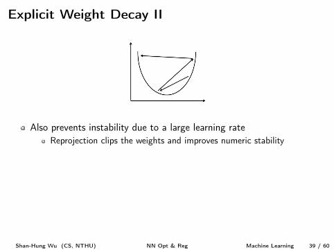
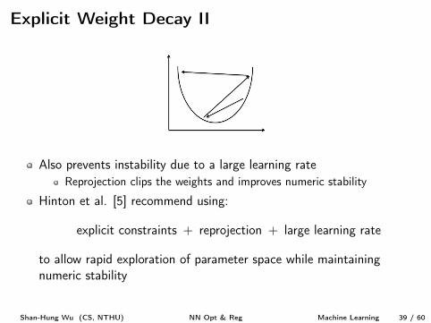
Also prevents instability due to a large learning rateReprojection clips the weights and improves numeric stability
Hinton et al. [5] recommend using:
explicit constraints + reprojection + large learning rate
to allow rapid exploration of parameter space while maintainingnumeric stability
Shan-Hung Wu (CS, NTHU) NN Opt & Reg Machine Learning 39 / 60
Explicit Weight Decay II
Also prevents instability due to a large learning rateReprojection clips the weights and improves numeric stability
Hinton et al. [5] recommend using:
explicit constraints + reprojection + large learning rate
to allow rapid exploration of parameter space while maintainingnumeric stability
Shan-Hung Wu (CS, NTHU) NN Opt & Reg Machine Learning 39 / 60
Outline
1 OptimizationMomentum & Nesterov MomentumAdaGrad & RMSPropBatch NormalizationContinuation Methods & Curriculum Learning
2 RegularizationWeight DecayData AugmentationDropoutManifold RegularizationDomain-Specific Model Design
Shan-Hung Wu (CS, NTHU) NN Opt & Reg Machine Learning 40 / 60
Data Augmentation
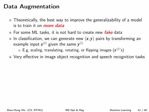
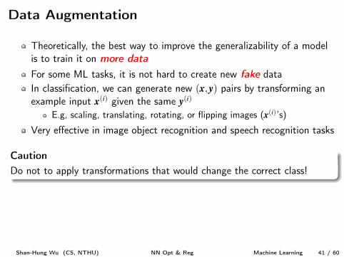
Theoretically, the best way to improve the generalizability of a modelis to train it on more data
For some ML tasks, it is not hard to create new fake dataIn classification, we can generate new (x,y) pairs by transforming anexample input x
(i) given the same y
(i)
E.g, scaling, translating, rotating, or flipping images (x(i)’s)
Very effective in image object recognition and speech recognition tasks
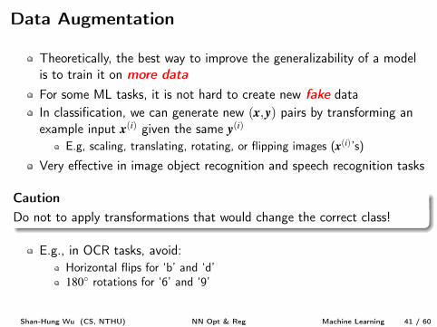
CautionDo not to apply transformations that would change the correct class!
E.g., in OCR tasks, avoid:Horizontal flips for ‘b’ and ‘d’180
� rotations for ‘6’ and ‘9’
Shan-Hung Wu (CS, NTHU) NN Opt & Reg Machine Learning 41 / 60
Data Augmentation
Theoretically, the best way to improve the generalizability of a modelis to train it on more data
For some ML tasks, it is not hard to create new fake dataIn classification, we can generate new (x,y) pairs by transforming anexample input x
(i) given the same y
(i)
E.g, scaling, translating, rotating, or flipping images (x(i)’s)
Very effective in image object recognition and speech recognition tasks
CautionDo not to apply transformations that would change the correct class!
E.g., in OCR tasks, avoid:Horizontal flips for ‘b’ and ‘d’180
� rotations for ‘6’ and ‘9’
Shan-Hung Wu (CS, NTHU) NN Opt & Reg Machine Learning 41 / 60
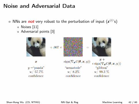
Noise and Adversarial Data
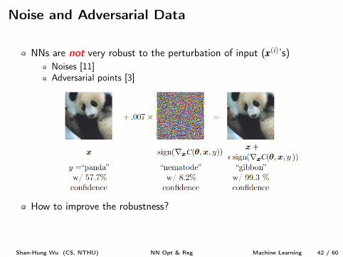
NNs are not very robust to the perturbation of input (x(i)’s)Noises [11]Adversarial points [3]
How to improve the robustness?
Shan-Hung Wu (CS, NTHU) NN Opt & Reg Machine Learning 42 / 60
Noise and Adversarial Data
NNs are not very robust to the perturbation of input (x(i)’s)Noises [11]Adversarial points [3]
How to improve the robustness?
Shan-Hung Wu (CS, NTHU) NN Opt & Reg Machine Learning 42 / 60

Noise Injection
We can train an NN with artificial random noise applied to x
(i)’s
Why noise injection works?Recall that the analytic solution of Ridge regression is
w =⇣
X
>X+a(t)
I
⌘�1
X
>y
In this case, weight decay = adding variance (noises)
More generally, makes the function f locally constant
Cost function C insensitive to small variations in weightsFinds solutions that are not merely minima, but minima surrounded byflat regions
Shan-Hung Wu (CS, NTHU) NN Opt & Reg Machine Learning 43 / 60

Noise Injection
We can train an NN with artificial random noise applied to x
(i)’sWhy noise injection works?
Recall that the analytic solution of Ridge regression is
w =⇣
X
>X+a(t)
I
⌘�1
X
>y
In this case, weight decay = adding variance (noises)
More generally, makes the function f locally constant
Cost function C insensitive to small variations in weightsFinds solutions that are not merely minima, but minima surrounded byflat regions
Shan-Hung Wu (CS, NTHU) NN Opt & Reg Machine Learning 43 / 60
Noise Injection
We can train an NN with artificial random noise applied to x
(i)’sWhy noise injection works?Recall that the analytic solution of Ridge regression is
w =⇣
X
>X+a(t)
I
⌘�1
X
>y
In this case, weight decay = adding variance (noises)
More generally, makes the function f locally constant
Cost function C insensitive to small variations in weightsFinds solutions that are not merely minima, but minima surrounded byflat regions
Shan-Hung Wu (CS, NTHU) NN Opt & Reg Machine Learning 43 / 60
Variants
We can also inject noise to hidden representations [8]Highly effective provided that the magnitude of the noise can becarefully tuned
The batch normalization, in addition to simplifying optimization, offerssimilar regularization effect to noise injection
Injects noises from examples in a minibatch to an activation a
(k)j
How about injecting noise to outputs (y(i)’s)?Already done in probabilistic models
Shan-Hung Wu (CS, NTHU) NN Opt & Reg Machine Learning 44 / 60
Variants
We can also inject noise to hidden representations [8]Highly effective provided that the magnitude of the noise can becarefully tuned
The batch normalization, in addition to simplifying optimization, offerssimilar regularization effect to noise injection
Injects noises from examples in a minibatch to an activation a
(k)j
How about injecting noise to outputs (y(i)’s)?
Already done in probabilistic models
Shan-Hung Wu (CS, NTHU) NN Opt & Reg Machine Learning 44 / 60
Variants
We can also inject noise to hidden representations [8]Highly effective provided that the magnitude of the noise can becarefully tuned
The batch normalization, in addition to simplifying optimization, offerssimilar regularization effect to noise injection
Injects noises from examples in a minibatch to an activation a
(k)j
How about injecting noise to outputs (y(i)’s)?Already done in probabilistic models
Shan-Hung Wu (CS, NTHU) NN Opt & Reg Machine Learning 44 / 60
Outline
1 OptimizationMomentum & Nesterov MomentumAdaGrad & RMSPropBatch NormalizationContinuation Methods & Curriculum Learning
2 RegularizationWeight DecayData AugmentationDropoutManifold RegularizationDomain-Specific Model Design
Shan-Hung Wu (CS, NTHU) NN Opt & Reg Machine Learning 45 / 60
Ensemble Methods
Ensemble methods can improve generalizability by offering differentexplanations to X
Voting: reduces variance of predictions if having independent votersBagging: resample X to makes voters less dependentBoosting: increase confidence (margin) of predictions, if not
overfitting
Ensemble methods in deep learning?Voting: train multiple NNsBagging: train multiple NNs, each with resampled X
GoogleLeNet [10], winner of ILSVRC’14, is an ensemble of 6 NNsVery time consuming to ensemble a large number of NNs
Shan-Hung Wu (CS, NTHU) NN Opt & Reg Machine Learning 46 / 60
Ensemble Methods
Ensemble methods can improve generalizability by offering differentexplanations to X
Voting: reduces variance of predictions if having independent voters
Bagging: resample X to makes voters less dependentBoosting: increase confidence (margin) of predictions, if not
overfitting
Ensemble methods in deep learning?Voting: train multiple NNsBagging: train multiple NNs, each with resampled X
GoogleLeNet [10], winner of ILSVRC’14, is an ensemble of 6 NNsVery time consuming to ensemble a large number of NNs
Shan-Hung Wu (CS, NTHU) NN Opt & Reg Machine Learning 46 / 60
Ensemble Methods
Ensemble methods can improve generalizability by offering differentexplanations to X
Voting: reduces variance of predictions if having independent votersBagging: resample X to makes voters less dependent
Boosting: increase confidence (margin) of predictions, if not
overfitting
Ensemble methods in deep learning?Voting: train multiple NNsBagging: train multiple NNs, each with resampled X
GoogleLeNet [10], winner of ILSVRC’14, is an ensemble of 6 NNsVery time consuming to ensemble a large number of NNs
Shan-Hung Wu (CS, NTHU) NN Opt & Reg Machine Learning 46 / 60
Ensemble Methods
Ensemble methods can improve generalizability by offering differentexplanations to X
Voting: reduces variance of predictions if having independent votersBagging: resample X to makes voters less dependentBoosting: increase confidence (margin) of predictions, if not
overfitting
Ensemble methods in deep learning?Voting: train multiple NNsBagging: train multiple NNs, each with resampled X
GoogleLeNet [10], winner of ILSVRC’14, is an ensemble of 6 NNsVery time consuming to ensemble a large number of NNs
Shan-Hung Wu (CS, NTHU) NN Opt & Reg Machine Learning 46 / 60
Ensemble Methods
Ensemble methods can improve generalizability by offering differentexplanations to X
Voting: reduces variance of predictions if having independent votersBagging: resample X to makes voters less dependentBoosting: increase confidence (margin) of predictions, if not
overfitting
Ensemble methods in deep learning?
Voting: train multiple NNsBagging: train multiple NNs, each with resampled X
GoogleLeNet [10], winner of ILSVRC’14, is an ensemble of 6 NNsVery time consuming to ensemble a large number of NNs
Shan-Hung Wu (CS, NTHU) NN Opt & Reg Machine Learning 46 / 60
Ensemble Methods
Ensemble methods can improve generalizability by offering differentexplanations to X
Voting: reduces variance of predictions if having independent votersBagging: resample X to makes voters less dependentBoosting: increase confidence (margin) of predictions, if not
overfitting
Ensemble methods in deep learning?Voting: train multiple NNs
Bagging: train multiple NNs, each with resampled XGoogleLeNet [10], winner of ILSVRC’14, is an ensemble of 6 NNsVery time consuming to ensemble a large number of NNs
Shan-Hung Wu (CS, NTHU) NN Opt & Reg Machine Learning 46 / 60
Ensemble Methods
Ensemble methods can improve generalizability by offering differentexplanations to X
Voting: reduces variance of predictions if having independent votersBagging: resample X to makes voters less dependentBoosting: increase confidence (margin) of predictions, if not
overfitting
Ensemble methods in deep learning?Voting: train multiple NNsBagging: train multiple NNs, each with resampled X
GoogleLeNet [10], winner of ILSVRC’14, is an ensemble of 6 NNsVery time consuming to ensemble a large number of NNs
Shan-Hung Wu (CS, NTHU) NN Opt & Reg Machine Learning 46 / 60
Ensemble Methods
Ensemble methods can improve generalizability by offering differentexplanations to X
Voting: reduces variance of predictions if having independent votersBagging: resample X to makes voters less dependentBoosting: increase confidence (margin) of predictions, if not
overfitting
Ensemble methods in deep learning?Voting: train multiple NNsBagging: train multiple NNs, each with resampled X
GoogleLeNet [10], winner of ILSVRC’14, is an ensemble of 6 NNs
Very time consuming to ensemble a large number of NNs
Shan-Hung Wu (CS, NTHU) NN Opt & Reg Machine Learning 46 / 60
Ensemble Methods
Ensemble methods can improve generalizability by offering differentexplanations to X
Voting: reduces variance of predictions if having independent votersBagging: resample X to makes voters less dependentBoosting: increase confidence (margin) of predictions, if not
overfitting
Ensemble methods in deep learning?Voting: train multiple NNsBagging: train multiple NNs, each with resampled X
GoogleLeNet [10], winner of ILSVRC’14, is an ensemble of 6 NNsVery time consuming to ensemble a large number of NNs
Shan-Hung Wu (CS, NTHU) NN Opt & Reg Machine Learning 46 / 60
Dropout I
Dropout: a feature-basedbagging
Resamples input aswell as latent featuresWith parameter
sharing among voters
SGD training: each time loading a minibatch, randomly sample abinary mask to apply to all input and hidden units
Each unit has probability a to be included (a hyperparameter)Typically, 0.8 for input units and 0.5 for hidden units
Different minibatches are used to train different parts of the NNSimilar to bagging, but much more efficientNo need to retrain unmasked unitsExponential number of voters
Shan-Hung Wu (CS, NTHU) NN Opt & Reg Machine Learning 47 / 60
Dropout I
Dropout: a feature-basedbagging
Resamples input aswell as latent features
With parameter
sharing among voters
SGD training: each time loading a minibatch, randomly sample abinary mask to apply to all input and hidden units
Each unit has probability a to be included (a hyperparameter)Typically, 0.8 for input units and 0.5 for hidden units
Different minibatches are used to train different parts of the NNSimilar to bagging, but much more efficientNo need to retrain unmasked unitsExponential number of voters
Shan-Hung Wu (CS, NTHU) NN Opt & Reg Machine Learning 47 / 60
Dropout I
Dropout: a feature-basedbagging
Resamples input aswell as latent featuresWith parameter
sharing among voters
SGD training: each time loading a minibatch, randomly sample abinary mask to apply to all input and hidden units
Each unit has probability a to be included (a hyperparameter)Typically, 0.8 for input units and 0.5 for hidden units
Different minibatches are used to train different parts of the NNSimilar to bagging, but much more efficientNo need to retrain unmasked unitsExponential number of voters
Shan-Hung Wu (CS, NTHU) NN Opt & Reg Machine Learning 47 / 60
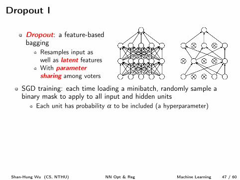
Dropout I
Dropout: a feature-basedbagging
Resamples input aswell as latent featuresWith parameter
sharing among voters
SGD training: each time loading a minibatch, randomly sample abinary mask to apply to all input and hidden units
Each unit has probability a to be included (a hyperparameter)
Typically, 0.8 for input units and 0.5 for hidden unitsDifferent minibatches are used to train different parts of the NN
Similar to bagging, but much more efficientNo need to retrain unmasked unitsExponential number of voters
Shan-Hung Wu (CS, NTHU) NN Opt & Reg Machine Learning 47 / 60
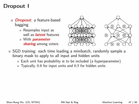
Dropout I
Dropout: a feature-basedbagging
Resamples input aswell as latent featuresWith parameter
sharing among voters
SGD training: each time loading a minibatch, randomly sample abinary mask to apply to all input and hidden units
Each unit has probability a to be included (a hyperparameter)Typically, 0.8 for input units and 0.5 for hidden units
Different minibatches are used to train different parts of the NNSimilar to bagging, but much more efficientNo need to retrain unmasked unitsExponential number of voters
Shan-Hung Wu (CS, NTHU) NN Opt & Reg Machine Learning 47 / 60
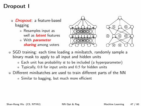
Dropout I
Dropout: a feature-basedbagging
Resamples input aswell as latent featuresWith parameter
sharing among voters
SGD training: each time loading a minibatch, randomly sample abinary mask to apply to all input and hidden units
Each unit has probability a to be included (a hyperparameter)Typically, 0.8 for input units and 0.5 for hidden units
Different minibatches are used to train different parts of the NNSimilar to bagging, but much more efficient
No need to retrain unmasked unitsExponential number of voters
Shan-Hung Wu (CS, NTHU) NN Opt & Reg Machine Learning 47 / 60
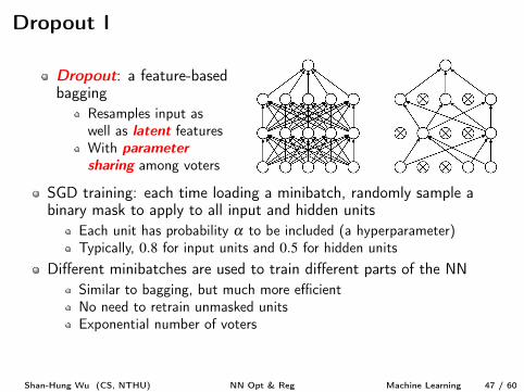
Dropout I
Dropout: a feature-basedbagging
Resamples input aswell as latent featuresWith parameter
sharing among voters
SGD training: each time loading a minibatch, randomly sample abinary mask to apply to all input and hidden units
Each unit has probability a to be included (a hyperparameter)Typically, 0.8 for input units and 0.5 for hidden units
Different minibatches are used to train different parts of the NNSimilar to bagging, but much more efficientNo need to retrain unmasked unitsExponential number of voters
Shan-Hung Wu (CS, NTHU) NN Opt & Reg Machine Learning 47 / 60

Dropout II
How to vote to make a final prediction?
Mask sampling:1 Randomly sample some (typically, 10⇠ 20) masks2 For each mask, apply it to the trained NN and get a prediction3 Average the predictions
Weigh scaling:Make a single prediction using the NN with all unitsBut weights going out from a unit is multiplied by aHeuristic: each unit outputs the same expected amount of weight as intraining
The better one is problem dependent
Shan-Hung Wu (CS, NTHU) NN Opt & Reg Machine Learning 48 / 60
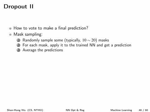
Dropout II
How to vote to make a final prediction?Mask sampling:
1 Randomly sample some (typically, 10⇠ 20) masks2 For each mask, apply it to the trained NN and get a prediction3 Average the predictions
Weigh scaling:Make a single prediction using the NN with all unitsBut weights going out from a unit is multiplied by aHeuristic: each unit outputs the same expected amount of weight as intraining
The better one is problem dependent
Shan-Hung Wu (CS, NTHU) NN Opt & Reg Machine Learning 48 / 60
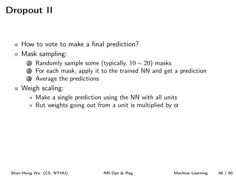
Dropout II
How to vote to make a final prediction?Mask sampling:
1 Randomly sample some (typically, 10⇠ 20) masks2 For each mask, apply it to the trained NN and get a prediction3 Average the predictions
Weigh scaling:Make a single prediction using the NN with all unitsBut weights going out from a unit is multiplied by a
Heuristic: each unit outputs the same expected amount of weight as intraining
The better one is problem dependent
Shan-Hung Wu (CS, NTHU) NN Opt & Reg Machine Learning 48 / 60
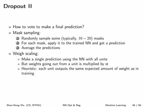
Dropout II
How to vote to make a final prediction?Mask sampling:
1 Randomly sample some (typically, 10⇠ 20) masks2 For each mask, apply it to the trained NN and get a prediction3 Average the predictions
Weigh scaling:Make a single prediction using the NN with all unitsBut weights going out from a unit is multiplied by aHeuristic: each unit outputs the same expected amount of weight as intraining
The better one is problem dependent
Shan-Hung Wu (CS, NTHU) NN Opt & Reg Machine Learning 48 / 60
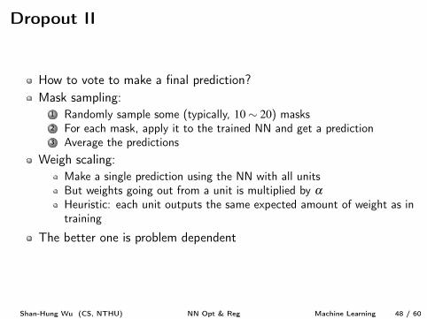
Dropout II
How to vote to make a final prediction?Mask sampling:
1 Randomly sample some (typically, 10⇠ 20) masks2 For each mask, apply it to the trained NN and get a prediction3 Average the predictions
Weigh scaling:Make a single prediction using the NN with all unitsBut weights going out from a unit is multiplied by aHeuristic: each unit outputs the same expected amount of weight as intraining
The better one is problem dependent
Shan-Hung Wu (CS, NTHU) NN Opt & Reg Machine Learning 48 / 60
Dropout III
Dropout improves generalization beyond ensembling
For example, in face image recognition:If there is a unit that detects noseDropping the unit encourages the model to learn mouth (or noseagain) in another unit
Shan-Hung Wu (CS, NTHU) NN Opt & Reg Machine Learning 49 / 60
Dropout III
Dropout improves generalization beyond ensemblingFor example, in face image recognition:
If there is a unit that detects noseDropping the unit encourages the model to learn mouth (or noseagain) in another unit
Shan-Hung Wu (CS, NTHU) NN Opt & Reg Machine Learning 49 / 60
Dropout III
Dropout improves generalization beyond ensemblingFor example, in face image recognition:If there is a unit that detects nose
Dropping the unit encourages the model to learn mouth (or noseagain) in another unit
Shan-Hung Wu (CS, NTHU) NN Opt & Reg Machine Learning 49 / 60
Dropout III
Dropout improves generalization beyond ensemblingFor example, in face image recognition:If there is a unit that detects noseDropping the unit encourages the model to learn mouth (or noseagain) in another unit
Shan-Hung Wu (CS, NTHU) NN Opt & Reg Machine Learning 49 / 60
Outline
1 OptimizationMomentum & Nesterov MomentumAdaGrad & RMSPropBatch NormalizationContinuation Methods & Curriculum Learning
2 RegularizationWeight DecayData AugmentationDropoutManifold RegularizationDomain-Specific Model Design
Shan-Hung Wu (CS, NTHU) NN Opt & Reg Machine Learning 50 / 60

Manifolds IOne way to improve the generalizability of a model is to incorporatethe prior knowledge
In many applications, data of the same class concentrate around oneor more low-dimensional manifolds
A manifold is a topological space that are linear locally
Shan-Hung Wu (CS, NTHU) NN Opt & Reg Machine Learning 51 / 60
Manifolds IOne way to improve the generalizability of a model is to incorporatethe prior knowledgeIn many applications, data of the same class concentrate around oneor more low-dimensional manifolds
A manifold is a topological space that are linear locally
Shan-Hung Wu (CS, NTHU) NN Opt & Reg Machine Learning 51 / 60
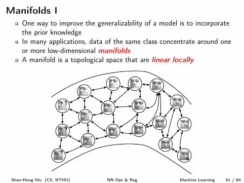
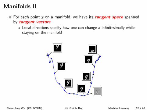
Manifolds II
For each point x on a manifold, we have its tangent space spannedby tangent vectors
Local directions specify how one can change x infinitesimally whilestaying on the manifold
Shan-Hung Wu (CS, NTHU) NN Opt & Reg Machine Learning 52 / 60
Tangent Prop
How to incorporate the manifold prior into a model?
Suppose we have the tangent vectors {v
(i,j)}j
for each example x
(i)
Tangent Prop [9] trains an NN classifier f with cost penalty:
W[f ] = Âi,j
—x
f (x(i))>v
(i,j)
To make f local constant along tangent directions
How to obtain {v
(i,j)}j
?Manually specified based on domain knowledge
Images: scaling, translating, rotating, flipping etc.
Or learned automatically (to be discussed later)
Shan-Hung Wu (CS, NTHU) NN Opt & Reg Machine Learning 53 / 60
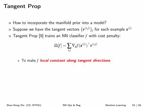
Tangent Prop
How to incorporate the manifold prior into a model?Suppose we have the tangent vectors {v
(i,j)}j
for each example x
(i)
Tangent Prop [9] trains an NN classifier f with cost penalty:
W[f ] = Âi,j
—x
f (x(i))>v
(i,j)
To make f local constant along tangent directions
How to obtain {v
(i,j)}j
?Manually specified based on domain knowledge
Images: scaling, translating, rotating, flipping etc.
Or learned automatically (to be discussed later)
Shan-Hung Wu (CS, NTHU) NN Opt & Reg Machine Learning 53 / 60
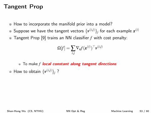
Tangent Prop
How to incorporate the manifold prior into a model?Suppose we have the tangent vectors {v
(i,j)}j
for each example x
(i)
Tangent Prop [9] trains an NN classifier f with cost penalty:
W[f ] = Âi,j
—x
f (x(i))>v
(i,j)
To make f local constant along tangent directions
How to obtain {v
(i,j)}j
?
Manually specified based on domain knowledgeImages: scaling, translating, rotating, flipping etc.
Or learned automatically (to be discussed later)
Shan-Hung Wu (CS, NTHU) NN Opt & Reg Machine Learning 53 / 60
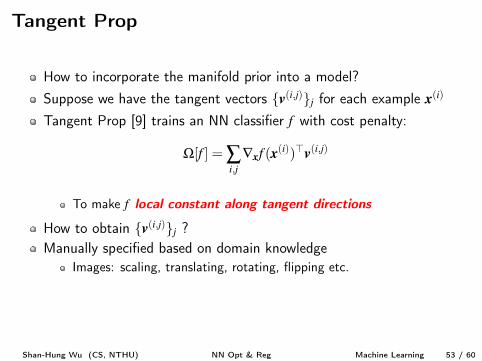
Tangent Prop
How to incorporate the manifold prior into a model?Suppose we have the tangent vectors {v
(i,j)}j
for each example x
(i)
Tangent Prop [9] trains an NN classifier f with cost penalty:
W[f ] = Âi,j
—x
f (x(i))>v
(i,j)
To make f local constant along tangent directions
How to obtain {v
(i,j)}j
?Manually specified based on domain knowledge
Images: scaling, translating, rotating, flipping etc.
Or learned automatically (to be discussed later)
Shan-Hung Wu (CS, NTHU) NN Opt & Reg Machine Learning 53 / 60
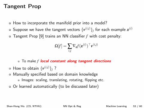
Tangent Prop
How to incorporate the manifold prior into a model?Suppose we have the tangent vectors {v
(i,j)}j
for each example x
(i)
Tangent Prop [9] trains an NN classifier f with cost penalty:
W[f ] = Âi,j
—x
f (x(i))>v
(i,j)
To make f local constant along tangent directions
How to obtain {v
(i,j)}j
?Manually specified based on domain knowledge
Images: scaling, translating, rotating, flipping etc.
Or learned automatically (to be discussed later)
Shan-Hung Wu (CS, NTHU) NN Opt & Reg Machine Learning 53 / 60
Outline
1 OptimizationMomentum & Nesterov MomentumAdaGrad & RMSPropBatch NormalizationContinuation Methods & Curriculum Learning
2 RegularizationWeight DecayData AugmentationDropoutManifold RegularizationDomain-Specific Model Design
Shan-Hung Wu (CS, NTHU) NN Opt & Reg Machine Learning 54 / 60
Domain-Specific Prior Knowledge
If done right, incorporating the domain-specific prior knowledge into amodel is a highly effective way the improve generalizability
Better f that “makes sense”May also simplify optimization problem
Shan-Hung Wu (CS, NTHU) NN Opt & Reg Machine Learning 55 / 60
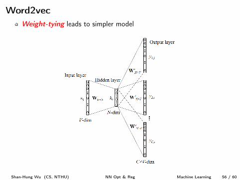
Word2vecWeight-tying leads to simpler model
Shan-Hung Wu (CS, NTHU) NN Opt & Reg Machine Learning 56 / 60
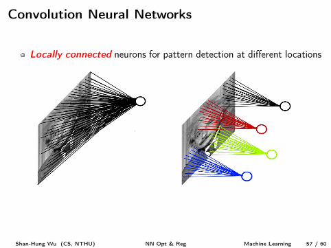
Convolution Neural Networks
Locally connected neurons for pattern detection at different locations
Shan-Hung Wu (CS, NTHU) NN Opt & Reg Machine Learning 57 / 60
Reference I
[1] Yoshua Bengio, Jérôme Louradour, Ronan Collobert, and JasonWeston.Curriculum learning.In Proceedings of the 26th annual international conference on machine
learning, pages 41–48. ACM, 2009.
[2] Anna Choromanska, Mikael Henaff, Michael Mathieu, Gérard BenArous, and Yann LeCun.The loss surfaces of multilayer networks.In AISTATS, 2015.
[3] Ian J Goodfellow, Jonathon Shlens, and Christian Szegedy.Explaining and harnessing adversarial examples.arXiv preprint arXiv:1412.6572, 2014.
[4] Ian J Goodfellow, Oriol Vinyals, and Andrew M Saxe.Qualitatively characterizing neural network optimization problems.arXiv preprint arXiv:1412.6544, 2014.
Shan-Hung Wu (CS, NTHU) NN Opt & Reg Machine Learning 58 / 60
Reference II
[5] Geoffrey E Hinton, Nitish Srivastava, Alex Krizhevsky, Ilya Sutskever,and Ruslan R Salakhutdinov.Improving neural networks by preventing co-adaptation of featuredetectors.arXiv preprint arXiv:1207.0580, 2012.
[6] Sergey Ioffe and Christian Szegedy.Batch normalization: Accelerating deep network training by reducinginternal covariate shift.arXiv preprint arXiv:1502.03167, 2015.
[7] Diederik Kingma and Jimmy Ba.Adam: A method for stochastic optimization.arXiv preprint arXiv:1412.6980, 2014.
[8] Ben Poole, Jascha Sohl-Dickstein, and Surya Ganguli.Analyzing noise in autoencoders and deep networks.arXiv preprint arXiv:1406.1831, 2014.
Shan-Hung Wu (CS, NTHU) NN Opt & Reg Machine Learning 59 / 60
Reference III
[9] Patrice Simard, Bernard Victorri, Yann LeCun, and John S Denker.Tangent prop-a formalism for specifying selected invariances in anadaptive network.In NIPS, volume 91, pages 895–903, 1991.
[10] Christian Szegedy, Wei Liu, Yangqing Jia, Pierre Sermanet, ScottReed, Dragomir Anguelov, Dumitru Erhan, Vincent Vanhoucke, andAndrew Rabinovich.Going deeper with convolutions.In Proceedings of the IEEE Conference on Computer Vision and
Pattern Recognition, pages 1–9, 2015.
[11] Yichuan Tang and Chris Eliasmith.Deep networks for robust visual recognition.In Proceedings of the 27th International Conference on Machine
Learning (ICML-10), pages 1055–1062, 2010.
Shan-Hung Wu (CS, NTHU) NN Opt & Reg Machine Learning 60 / 60


![Unsupervised Adaptive Neural Network Regularization for ...optimization routines, e.g, the ADAM optimizer [23]. (R2) Reconstruction update: After having obtained an esti-mate for ,](https://img.pdfslide.net/doc/110x75/6006950609c81230385f83c7/unsupervised-adaptive-neural-network-regularization-for-optimization-routines.jpg)


![Global Optimality in Neural Network Training · •Adapt network architecture to data [1] Optimization Generalization/ Regularization Architecture [1] Bengio, et al., “onvex neural](https://img.pdfslide.net/doc/110x75/603ef56c7ebe3d37046c1be3/global-optimality-in-neural-network-aadapt-network-architecture-to-data-1-optimization.jpg)