Nc

Ia

b

a

ARRAA

KNEFIR

1

ch[ailtgiatC

a

h1

Applied Soft Computing 21 (2014) 95–106

Contents lists available at ScienceDirect

Applied Soft Computing

j ourna l h o mepage: www.elsev ier .com/ locate /asoc

euro-fuzzy techniques to optimize an FPGA embeddedontroller for robot navigation

luminada Baturonea,1, Andrés Gersnoviezb,∗, Ángel Barrigaa

Dept. de Electrónica y Electromagnetismo, Univ. of Seville, and the Instituto de Microelectrónica de Sevilla (IMSE-CNM-CSIC), Seville, SpainDept. de Arquitectura de Computadores, Electrónica y Tecnología Electrónica, Univ. of Cordoba, Cordoba, Spain

r t i c l e i n f o

rticle history:eceived 28 August 2012eceived in revised form 18 January 2014ccepted 3 March 2014vailable online 26 March 2014

eywords:euro-fuzzy techniquesmbedded systemsPGA implementationntelligent control

a b s t r a c t

This paper describes how low-cost embedded controllers for robot navigation can be obtained byusing a small number of if-then rules (exploiting the connection in cascade of rule bases) that applyTakagi–Sugeno fuzzy inference method and employ fuzzy sets represented by normalized triangularfunctions. The rules comprise heuristic and fuzzy knowledge together with numerical data obtainedfrom a geometric analysis of the control problem that considers the kinematic and dynamic constraintsof the robot. Numerical data allow tuning the fuzzy symbols used in the rules to optimize the controllerperformance. From the implementation point of view, very few computational and memory resourcesare required: standard logical, addition, and multiplication operations and a few data that can be rep-resented by integer values. This is illustrated with the design of a controller for the safe navigation ofan autonomous car-like robot among possible obstacles toward a goal configuration. Implementation

obot navigation results of an FPGA embedded system based on a general-purpose soft processor confirm that percentagereduction in clock cycles is drastic thanks to applying the proposed neuro-fuzzy techniques. Simulationand experimental results obtained with the robot confirm the efficiency of the controller designed. Designmethodology has been supported by the CAD tools of the environment Xfuzzy 3 and by the EmbeddedSystem Tools from Xilinx.

© 2014 Elsevier B.V. All rights reserved.

. Introduction

Fuzzy rule-based systems have been successfully used in manyontrol applications thanks to their capability to deal with theeuristic knowledge of an expert that is expressed linguistically1–4]. Linguistic if-then rules including imprecise and maybembiguous terms are translated rather easily into if-then rulesncluding fuzzy sets. The capability of fuzzy systems to manageinguistic information facilitates not only the development of con-rollers but also their debugging and maintenance. Due to thereat use of fuzzy systems in control engineering, different types ofmplementations for these systems have been proposed in the liter-ture [5]. These approaches range from software implementations

o hardware realizations by ASICs (Application Specific Integratedircuits) or FPGAs (Field Programmable Gate Arrays).

∗ Corresponding author. Tel.: +34 957212224.E-mail addresses: lumi@imse-cnm.csic.es (I. Baturone),

ndresgm@uco.es (A. Gersnoviez), barriga@imse-cnm.csic.es (Á. Barriga).1 Tel.: +34 95446666; fax: +34 95446600.

ttp://dx.doi.org/10.1016/j.asoc.2014.03.001568-4946/© 2014 Elsevier B.V. All rights reserved.

The development of complex systems for industrial con-trol applications demands high speed, low power and areaconsumption, and low cost. The solution to satisfy theserequirements is the implementation as embedded systems [6].Implementation on ASICs satisfies these requirements, but due tothe high initial engineering cost, ASICs are adequate when they aremanufactured in high quantity. A good alternative is the implemen-tation on FPGAs. An FPGA can be fully programmable to generate aspecific hardware that matches the requirements of the user. Thegreat advantages of these devices compared to ASICs are its flexi-bility, a shorter time-to-market and a lower cost if the number offabricated devices is small. Modern FPGA families include a highnumber of specific resources and provide powerful and friendlyCAD tools that allow the development of complex embedded sys-tems [7–19]. FPGA manufacturers also allow the implementationof efficient 32-bit RISC processors, such as the MicroBlaze systemfrom Xilinx and the Nios processor from Altera.

The continuous evolution of programmable devices has

increased the use of FPGAs as platforms for the development offuzzy systems [12–19]. Some of these FPGA implementations offuzzy controllers are used to control autonomous mobile robots[16–19]. Current research in robotics concerns with multi-robot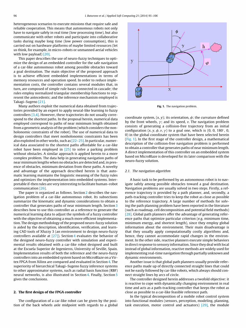

9 oft Computing 21 (2014) 95–106

hrhctcuw

moaimmtrrT

tcsefhdairwcneamapc

iscdnwtiictmaIctstng

2

t

6 I. Baturone et al. / Applied S

eterogeneous scenarios to execute missions that require safe andeliable cooperation. This means that autonomous robots not onlyave to navigate safely in real time (low processing time), but alsoommunicate with other robots and participate into collaborativeasks during maybe long time (low power consumption), this isarried out on hardware platforms of maybe limited resources (lets think, for example, in micro-robots or unmanned aerial vehiclesith low payload) [20].

This paper describes the use of neuro-fuzzy techniques to opti-ize the design of an embedded controller for the safe navigation

f a car-like autonomous robot among possible obstacles toward goal destination. The main objective of the proposed approachs to achieve efficient embedded implementations in terms of

emory resources and operation speed. In order to reduce imple-entation costs, the controller contains several modules that, in

urn, are composed of simple rule bases connected in cascade; theules employ normalized triangular membership functions to rep-esent the antecedents; and the inference mechanism employed isakagi–Sugeno [21].

Many authors exploit the numerical data obtained from trajec-ories provided by an expert to apply neural-like learning to fuzzyontrollers [3,4]. However, these trajectories do not usually corre-pond to the shortest paths. In the proposal herein, numerical datamployed correspond to paths of near minimum length obtainedrom a geometric analysis of the problem (which considers the non-olonomic constraints of the robot). The use of numerical data toesign controllers that meet nonholonomic constraints has beenlso exploited in other works, such as [22–25]. In particular, numer-cal data associated to the shortest paths affordable for a car-likeobot have been employed in [25] to solve a parking problemithout obstacles. A similar approach is applied herein to a more

omplex problem. The data help in generating navigation paths ofear minimum lengths when no obstacles are detected and, in pres-nce of obstacles, minimum deviation from these paths. A noveltynd advantage of the approach described herein is that auto-atic learning maintains the linguistic meaning of the fuzzy rules

nd optimizes the implementation into embedded systems. Inter-retable if-then rules are very interesting to facilitate human–robotommunication [26].

The paper is organized as follows. Section 2 describes the nav-gation problem of a car-like autonomous robot. Its subsectionsummarize the kinematic and dynamic considerations to obtain aontroller that generates paths of near minimum length. Section 3escribes how to use this controller as a reference to generate theumerical learning data to adjust the symbols of a fuzzy controllerith the objective of obtaining a much more efficient implementa-

ion. The design methodology of the proposed neuro-fuzzy solutions aided by the description, identification, verification, and learn-ng CAD tools of Xfuzzy 3 (an environment to design neuro-fuzzyontrollers available at [27]). Section 4 evaluates the behavior ofhe designed neuro-fuzzy controller with simulation and experi-

ental results obtained with a car-like robot designed and builtt the Escuela Superior de Ingenieros, University of Seville, Spain.mplementation results of both the reference and the neuro-fuzzyontrollers into an embedded system based on MicroBlaze on a Vir-ex FPGA from Xilinx are compared and evaluated in Section 4. Theuperiority of hierarchical Takagi–Sugeno fuzzy inference systemso other approximator systems, such as radial basis function (RBF)eural networks, is also illustrated in Section 4. Finally, Section 5ives the conclusions.

. The first design of the FPGA controller

The configuration of a car-like robot can be given by the posi-ion of the back wheels axle midpoint with regards to a global

Fig. 1. The navigation problem.

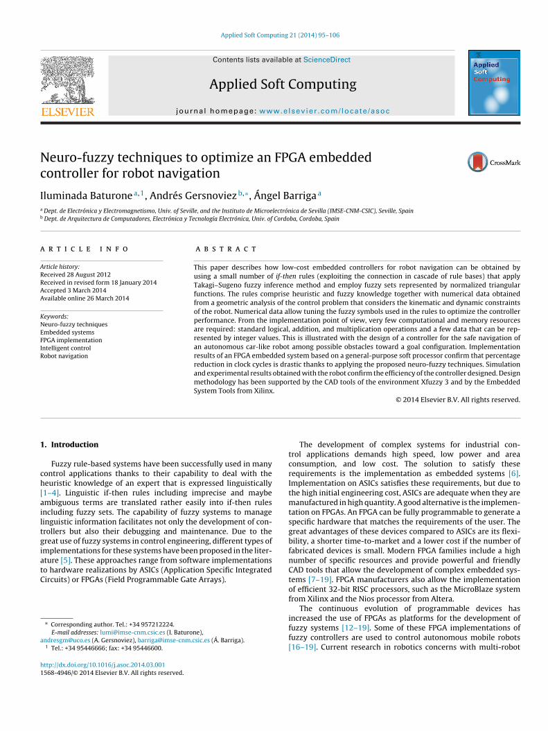
coordinate system, (x, y); its orientation, �; the curvature definedby the front wheels, �; and its speed, v. The navigation problemconsists of generating a collision-free trajectory from an initialconfiguration (x, y, �, v, �) to a goal one, which is (0, 0, 180◦, 0,0) in the global coordinate system that have been selected herein(Fig. 1). In the first stage of the controller design, a mathematicaldescription of the collision-free navigation problem is performedto obtain a controller that generates paths of near minimum length.A direct implementation of this controller on an embedded systembased on MicroBlaze is developed for its later comparison with theneuro-fuzzy solution.

2.1. The navigation algorithm

A basic task to be performed by an autonomous robot is to nav-igate safely among possible obstacles toward a goal destination.Navigation problems are usually solved in two steps. Firstly, a ref-erence trajectory is provided by a path planner, and, secondly, apath-tracking controller tries to keep the robot as close as possibleto the reference trajectory. A large number of methods for solv-ing the path planning problem have been reported in the literature(such as roadmap, cell decomposition and potential field methods)[28]. Global path planners offer the advantage of generating refer-ence paths that optimize particular criterion (e.g. minimum time,minimum energy, and shortest length), since they employ globalinformation about the environment. Their main disadvantage isthat they usually apply computationally costly algorithms and,hence, they cannot accommodate rapid changes in the environ-ment. In the other side, reactive planners execute simple behaviorsin direct response to sensory information. Since they deal with localinstead of global information, reactive methods are widely used forimplementing real-time navigation through partially unknown anddynamic environments.

Another issue is that global path planners usually provide refer-ence paths made up of directly connected straight lines that couldnot be easily followed by car-like robots, which always should con-nect straight lines by arcs of circle.

The controller designed herein addresses a twofold objective: itis reactive to cope with dynamically changing environment in realtime and acts as a path-tracking controller that keeps the robot as

close as possible to a car-like feasible reference path.

In the typical decomposition of a mobile robot control systeminto functional modules (sensors, perception, modeling, planning,task execution, motor control and actuators) [29], the module

oft Computing 21 (2014) 95–106 97

dapgcrcbpit

dtp1tawscs

h

1

2

3

ibatmcttvbcplimHtcs

fi

oc

I. Baturone et al. / Applied S

esigned herein would be in charge of reactive obstacle avoidancend path-tracking tasks. It can be combined with a global pathlanner in charge of modeling and planning in order to optimizelobal criterion (taking into account the overall obstacles spatialonfiguration and characteristics of the whole space where theobot can move). A review of such hybrid architectures thatombine global (deliberative) with local (reactive) modules cane seen in [30]. For example, a global fuzzy behavior control isroposed in [17] to integrate several local modules. However, this

s out of the scope of this paper, which will focus on the design ofhe reactive obstacle avoidance and path-tracking module.

No model about the environment is used nor constructed by theesigned reactive controller but only the information provided byhe robot sensors. In particular, the sensor considered is a 2-D laserlaced at the robot front part. The laser performs a scan of up to80 degrees of the space in the front of the robot and identifieshe points of possible obstacles by their distance, h, and sweepingngle, ϕ (Fig. 1). Of course, the robot could drive backward in a safeay by making use of sensors placed at the robot back part that

can the space in the back of the robot. However, for the sake oflarity, the robot is considered herein to drive always forward or totop.

The coarse structure of the reactive controller is obtained fromeuristic knowledge expressed linguistically, as follows:

. If there is an obstacle very close to the robot, the robot shouldstop to avoid collision.2

. If there is an obstacle close to the robot, a maneuver to avoid itshould be carried out, as follows3:(a) If the obstacle is on the right (left) then turn to the left (right).(b) If the obstacle is in front of the robot then:

• Turn to the same side as in the previous control cycle (pro-vided the obstacle was already detected).

• If this is the first time the obstacle is detected, apply theturning sign as no obstacle is detected.

. If the obstacles are far from the robot, there is no need to avoidthem (by the moment) and the robot should navigate toward thegoal configuration by the shortest path.

Several symbolic concepts appear in these rules (depicted intalic fonts) that need specification. They might be defined by mem-ership functions based on heuristics as well as trial and errorpproach. Doing that, the paths obtained will not be as good ashey could be. Our proposal is to consider the dynamic and kine-

atic constraints of the robot so as to optimally define the symboliconcepts. In particular, the car-like nonholonomic constraints makehat the movement direction must always be tangent to the trajec-ory and the turning radius is mechanically limited to a minimumalue, which is equivalent to say that the robot curvature is upperounded. In the absence of obstacles, the shortest paths for aar-like robot consist of a finite sequence of two elementary com-onents: arcs of circle (with minimum turning radius) and straight

ine segments [31,32]. In an environment cluttered by obstacles, its proven in [33] that shortest paths consist only of arcs of a circle of

inimum turning radius, line segments, and pieces of boundaries.

ence, an obstacle will be very close if the radius of the arc of circle

o avoid it should be smaller than the minimum. An obstacle will belose and should be avoided if it will be inside the area that will bewept by the robot when it travels along its path. In other case, the

2 If the robot would be provided with sensors in its rear, this would not be thenal action and the robot would drive backward, as commented above.3 In case this local module is combined with a global controller, the turning sign

f the maneuver defined by rules 2.a and 2.b could be determined by the globalontroller.

Fig. 2. Area of unavoidable obstacles.

obstacle is far and the controller has to provide the shortest pathmade of a finite sequence of arcs of circle with minimum turningradius and straight line segments (as illustrated in Fig. 1). This isanalyzed more in detail in the following.

2.2. Very close obstacles

Let us consider a coordinate system (xr, yr) attached to the robot,whose origin is placed at the back wheels axle midpoint (Fig. 2). Thecoordinates on an obstacle referred to that system are the follow-ing:

xro = d + h · sin ϕ yro = −h · cos ϕ (1)

where d is the distance of the laser to the back wheel axle (1.65 min the robot considered in the experiments).

Taking into account that the robot considered in our analysis hasa width of 1 m and the maximum speed considered is 1 m/s, 2 m atboth sides of the robot should be free of obstacles for safety pur-poses. An obstacle will be very close and, hence, unavoidable, if itenters the forbidden area (shadowed area in Fig. 2). Let us consideran obstacle placed on the right of the robot (ϕ ∈ [0◦, 90◦]), as shownin Fig. 2. It will be very close if the robot cannot avoid it by tur-ning to the left with an arc of circle with minimum turning radius(R = 1/|�max|), leaving 2 m of free space:

x2ro +

(yro − 1

|�max|)2

<(

1|�max| + 2

)2if ϕ ∈ [0◦, 90◦] (2)

Similarly, if the obstacle is placed on the left of the robot(ϕ ∈ [90◦, 180◦]), it will be very close if the robot cannot avoid itby turning to the right:

x2ro +

(yro + 1

|�max|)2

<(

1|�max| + 2

)2if ϕ ∈ [90◦, 180◦]

(3)

Grouping Eqs. (2) and (3), and substituting xro and yro by Eq. (1),

the area of very close or unavoidable obstacles is defined by:

(d + h · | sin ϕ|)2 +(

h · | cos ϕ| + 1|�max|

)2<(

1|�max| + 2

)2(4)

9 oft Co

in

2

wiolf(

dprc

asiwr

x

i

2

i(a

8 I. Baturone et al. / Applied S

Eq. (4) has been selected to describe very close obstacles, sincet uses the variables h and ϕ provided directly by the laser. Hence,o processing of laser data is required.

.3. Close obstacles

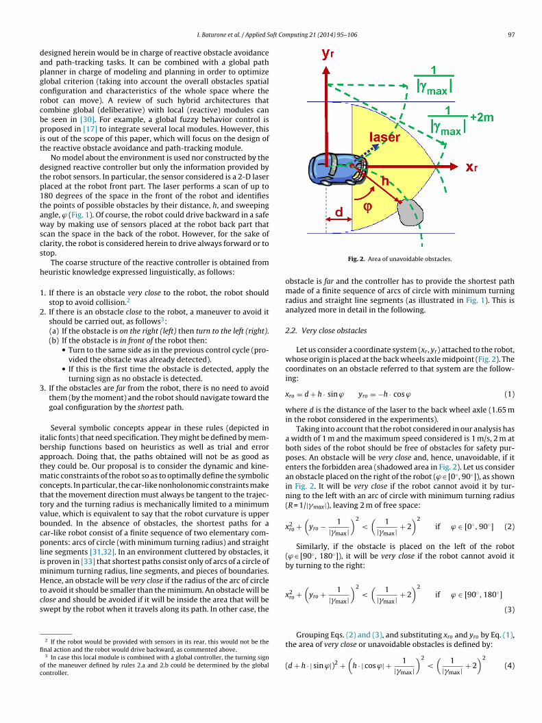
An obstacle will be close if it will be inside the safety area thatill be swept by the robot when it travels along its path. Taking

nto account the current robot curvature, � , a first condition for anbstacle to be close is to be less than 2 m on the right or on theeft along the arc of circle to be described by the robot (Fig. 3a), asollows:

1|� | − 2

)2< x2

ro +(

yro + 1|� |)2

<(

1|� | + 2

)2(5)

The safety area should also contain 2 m ahead in the drivingirection. Hence, let us consider a coordinate system (xR, yR) dis-laced 2 m in the driving direction and rotated an angle of 2� withespect to the coordinate system (xr, yr), as illustrated in Fig. 3b. Theoordinates of an obstacle referred to this system are the following:

xRo =(

xro − sin 2�

�

)cos 2� −

(yro + 1 − cos 2�

�

)sin 2�

yRo =(

xro − sin 2�

�

)sin 2� +

(yro + 1 − cos 2�

�

)cos 2�

(6)

A second condition for an obstacle to be close and, hence, to bevoided is that it becomes a very close obstacle in the future (darkhadowed area in Fig. 3a). This condition is easier to be expressedn the coordinate system (xR, yR). Similarly to Eqs. (2) and (3), it

ill be very close if their position with regards to the displaced andotated coordinate system verifies that:

2Ro +

(yRo + 1

|�max|)2

<(

1|�max| + 2

)2(7)

Finally, the third condition for a close obstacle is that, currently,t is not very close and, hence, it does not verify Eq. (4).

.4. Obstacle avoidance

The minimum magnitude of the curvature to avoid an obstacledentified as close is determined by the closest point of that obstaclewhose coordinates will be named hM and ϕM herein). Taking intoccount that a reference curvature is not adopted instantaneously

Fig. 3. (a) Area of close obstacles. (b) Transformation b

mputing 21 (2014) 95–106

by the robot but has a delay, a 4-m safety corridor has been con-sidered for selecting the minimum value of the curvature. Withsuch selection, the dynamic features of the robot considered in theexperiments allow the 2-m width corridor free of obstacles. Hence,the minimum magnitude of the curvature (similarly to Eq. (4)) isgiven by:

(d + hM · | sin ϕM |)2 +(

hM · | cos ϕM | + 1|� |)2

=(

1|� | + 4

)2(8)

From the formula above, the value of |� | can be obtained as:

|� | = 8 − 2hM · | cos ϕM |d2 + h2

M + 2hM · d · | sin ϕM | − 16(9)

The sign of the curvature when an obstacle is avoided is givenby the second if-then rule explained in Section 2.1 (the criterionadopted is that |� | = � , in the case of turning to the right, and|� | = − � , in the case of turning to the left).

2.5. Navigation toward the goal

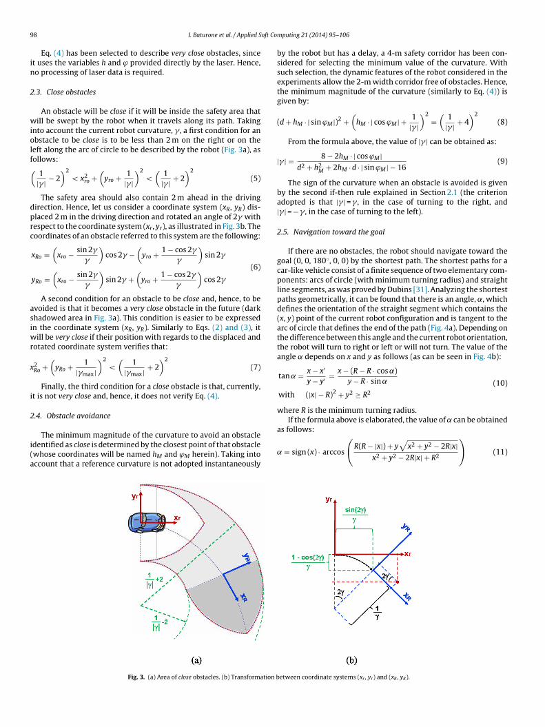
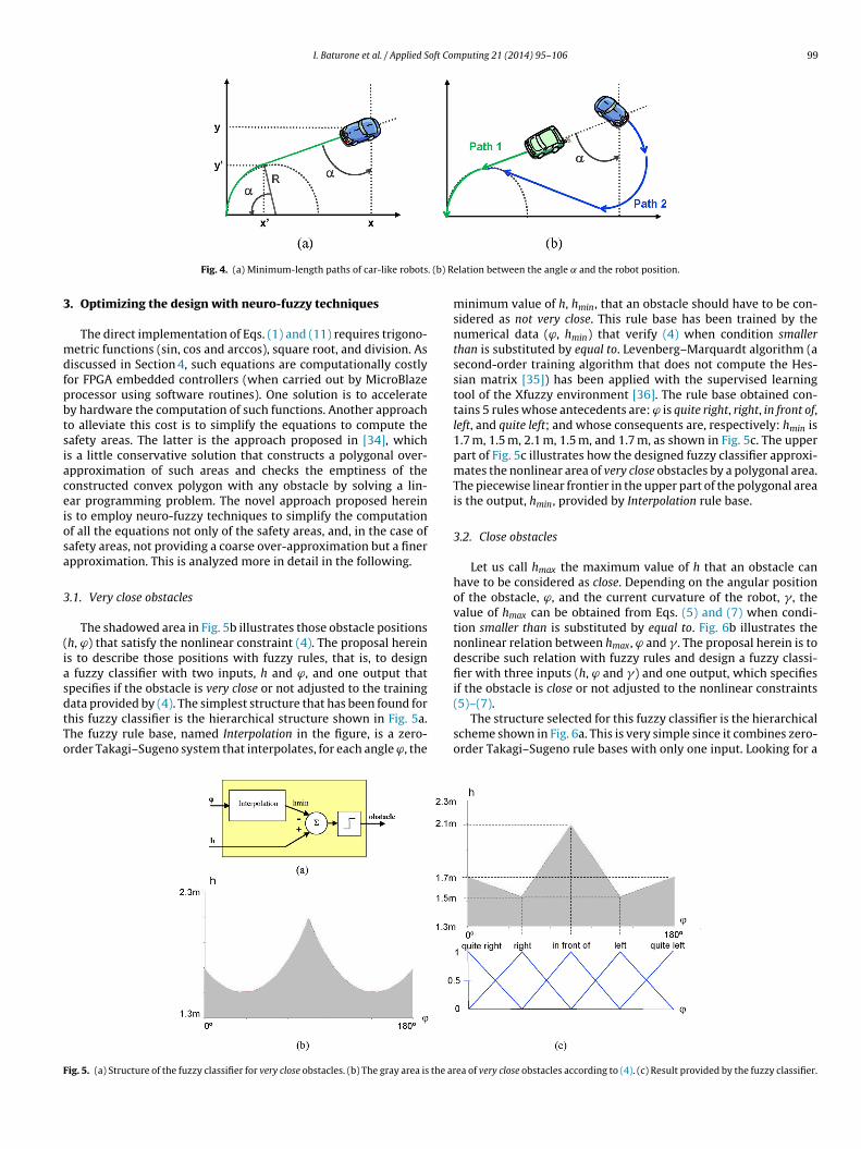
If there are no obstacles, the robot should navigate toward thegoal (0, 0, 180◦, 0, 0) by the shortest path. The shortest paths for acar-like vehicle consist of a finite sequence of two elementary com-ponents: arcs of circle (with minimum turning radius) and straightline segments, as was proved by Dubins [31]. Analyzing the shortestpaths geometrically, it can be found that there is an angle, ˛, whichdefines the orientation of the straight segment which contains the(x, y) point of the current robot configuration and is tangent to thearc of circle that defines the end of the path (Fig. 4a). Depending onthe difference between this angle and the current robot orientation,the robot will turn to right or left or will not turn. The value of theangle depends on x and y as follows (as can be seen in Fig. 4b):

tan = x − x′

y − y′ = x − (R − R · cos ˛)y − R · sin ˛

with (|x| − R)2 + y2 ≥ R2

(10)

where R is the minimum turning radius.If the formula above is elaborated, the value of can be obtained

as follows:

= sign (x) · arccos

(R(R − |x|) + y

√x2 + y2 − 2R|x|

x2 + y2 − 2R|x| + R2

)(11)

etween coordinate systems (xr , yr) and (xR , yR).

I. Baturone et al. / Applied Soft Computing 21 (2014) 95–106 99

. (b) R

3

mdfpbtsiaceiosa

3

(iasdtTo

F

Fig. 4. (a) Minimum-length paths of car-like robots

. Optimizing the design with neuro-fuzzy techniques

The direct implementation of Eqs. (1) and (11) requires trigono-etric functions (sin, cos and arccos), square root, and division. As

iscussed in Section 4, such equations are computationally costlyor FPGA embedded controllers (when carried out by MicroBlazerocessor using software routines). One solution is to acceleratey hardware the computation of such functions. Another approacho alleviate this cost is to simplify the equations to compute theafety areas. The latter is the approach proposed in [34], whichs a little conservative solution that constructs a polygonal over-pproximation of such areas and checks the emptiness of theonstructed convex polygon with any obstacle by solving a lin-ar programming problem. The novel approach proposed hereins to employ neuro-fuzzy techniques to simplify the computationf all the equations not only of the safety areas, and, in the case ofafety areas, not providing a coarse over-approximation but a finerpproximation. This is analyzed more in detail in the following.

.1. Very close obstacles

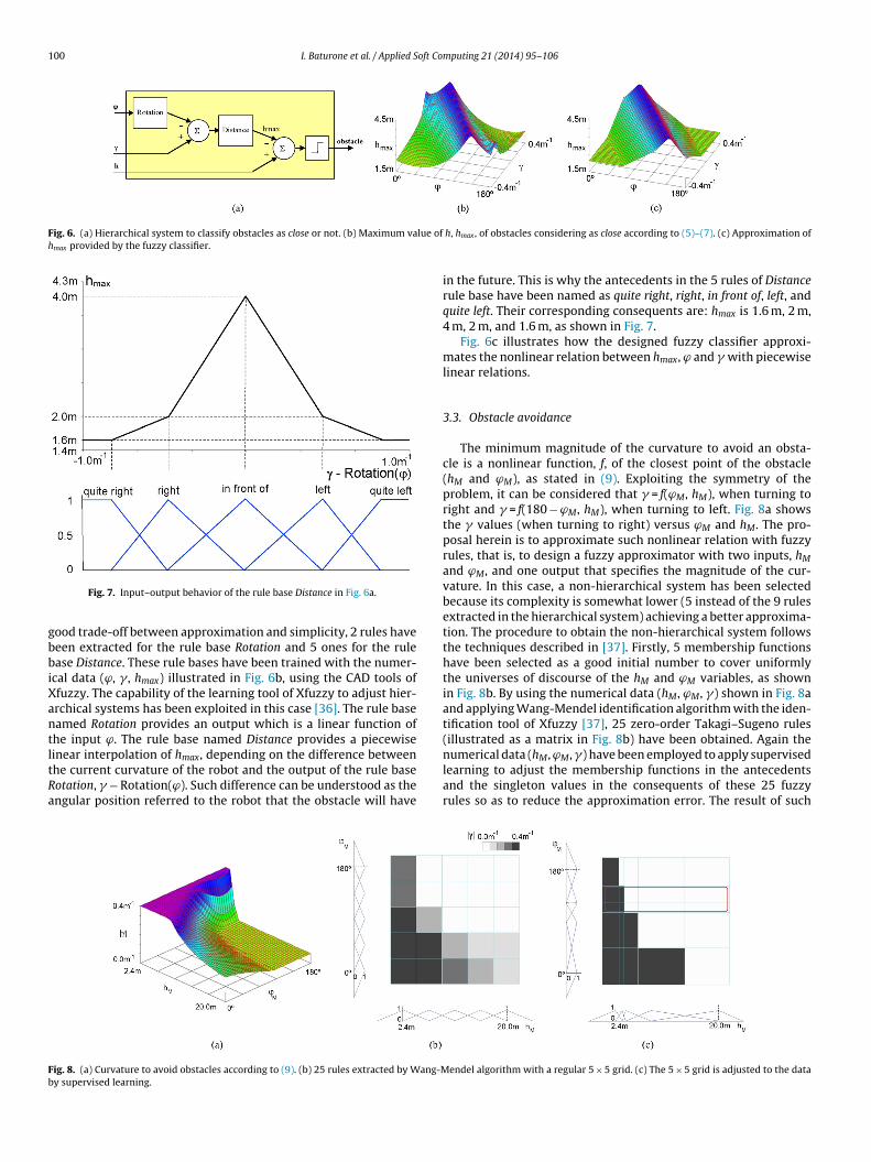
The shadowed area in Fig. 5b illustrates those obstacle positionsh, ϕ) that satisfy the nonlinear constraint (4). The proposal hereins to describe those positions with fuzzy rules, that is, to design

fuzzy classifier with two inputs, h and ϕ, and one output thatpecifies if the obstacle is very close or not adjusted to the training

ata provided by (4). The simplest structure that has been found forhis fuzzy classifier is the hierarchical structure shown in Fig. 5a.he fuzzy rule base, named Interpolation in the figure, is a zero-rder Takagi–Sugeno system that interpolates, for each angle ϕ, the

ig. 5. (a) Structure of the fuzzy classifier for very close obstacles. (b) The gray area is the ar

elation between the angle and the robot position.

minimum value of h, hmin, that an obstacle should have to be con-sidered as not very close. This rule base has been trained by thenumerical data (ϕ, hmin) that verify (4) when condition smallerthan is substituted by equal to. Levenberg–Marquardt algorithm (asecond-order training algorithm that does not compute the Hes-sian matrix [35]) has been applied with the supervised learningtool of the Xfuzzy environment [36]. The rule base obtained con-tains 5 rules whose antecedents are: ϕ is quite right, right, in front of,left, and quite left; and whose consequents are, respectively: hmin is1.7 m, 1.5 m, 2.1 m, 1.5 m, and 1.7 m, as shown in Fig. 5c. The upperpart of Fig. 5c illustrates how the designed fuzzy classifier approxi-mates the nonlinear area of very close obstacles by a polygonal area.The piecewise linear frontier in the upper part of the polygonal areais the output, hmin, provided by Interpolation rule base.

3.2. Close obstacles

Let us call hmax the maximum value of h that an obstacle canhave to be considered as close. Depending on the angular positionof the obstacle, ϕ, and the current curvature of the robot, � , thevalue of hmax can be obtained from Eqs. (5) and (7) when condi-tion smaller than is substituted by equal to. Fig. 6b illustrates thenonlinear relation between hmax, ϕ and � . The proposal herein is todescribe such relation with fuzzy rules and design a fuzzy classi-fier with three inputs (h, ϕ and �) and one output, which specifiesif the obstacle is close or not adjusted to the nonlinear constraints

(5)–(7).

The structure selected for this fuzzy classifier is the hierarchicalscheme shown in Fig. 6a. This is very simple since it combines zero-order Takagi–Sugeno rule bases with only one input. Looking for a

ea of very close obstacles according to (4). (c) Result provided by the fuzzy classifier.

100 I. Baturone et al. / Applied Soft Computing 21 (2014) 95–106

Fig. 6. (a) Hierarchical system to classify obstacles as close or not. (b) Maximum value ofhmax provided by the fuzzy classifier.

gbbiXantltRa

Fb

Fig. 7. Input–output behavior of the rule base Distance in Fig. 6a.

ood trade-off between approximation and simplicity, 2 rules haveeen extracted for the rule base Rotation and 5 ones for the rulease Distance. These rule bases have been trained with the numer-

cal data (ϕ, � , hmax) illustrated in Fig. 6b, using the CAD tools offuzzy. The capability of the learning tool of Xfuzzy to adjust hier-rchical systems has been exploited in this case [36]. The rule baseamed Rotation provides an output which is a linear function ofhe input ϕ. The rule base named Distance provides a piecewise

inear interpolation of hmax, depending on the difference betweenhe current curvature of the robot and the output of the rule baseotation, � − Rotation(ϕ). Such difference can be understood as thengular position referred to the robot that the obstacle will have

ig. 8. (a) Curvature to avoid obstacles according to (9). (b) 25 rules extracted by Wang-My supervised learning.

h, hmax , of obstacles considering as close according to (5)–(7). (c) Approximation of

in the future. This is why the antecedents in the 5 rules of Distancerule base have been named as quite right, right, in front of, left, andquite left. Their corresponding consequents are: hmax is 1.6 m, 2 m,4 m, 2 m, and 1.6 m, as shown in Fig. 7.

Fig. 6c illustrates how the designed fuzzy classifier approxi-mates the nonlinear relation between hmax, ϕ and � with piecewiselinear relations.

3.3. Obstacle avoidance

The minimum magnitude of the curvature to avoid an obsta-cle is a nonlinear function, f, of the closest point of the obstacle(hM and ϕM), as stated in (9). Exploiting the symmetry of theproblem, it can be considered that � = f(ϕM, hM), when turning toright and � = f(180 − ϕM, hM), when turning to left. Fig. 8a showsthe � values (when turning to right) versus ϕM and hM. The pro-posal herein is to approximate such nonlinear relation with fuzzyrules, that is, to design a fuzzy approximator with two inputs, hM

and ϕM, and one output that specifies the magnitude of the cur-vature. In this case, a non-hierarchical system has been selectedbecause its complexity is somewhat lower (5 instead of the 9 rulesextracted in the hierarchical system) achieving a better approxima-tion. The procedure to obtain the non-hierarchical system followsthe techniques described in [37]. Firstly, 5 membership functionshave been selected as a good initial number to cover uniformlythe universes of discourse of the hM and ϕM variables, as shownin Fig. 8b. By using the numerical data (hM, ϕM, �) shown in Fig. 8aand applying Wang-Mendel identification algorithm with the iden-tification tool of Xfuzzy [37], 25 zero-order Takagi–Sugeno rules(illustrated as a matrix in Fig. 8b) have been obtained. Again the

numerical data (hM, ϕM, �) have been employed to apply supervisedlearning to adjust the membership functions in the antecedentsand the singleton values in the consequents of these 25 fuzzyrules so as to reduce the approximation error. The result of such

endel algorithm with a regular 5 × 5 grid. (c) The 5 × 5 grid is adjusted to the data

I. Baturone et al. / Applied Soft Computing 21 (2014) 95–106 101

F in ϕM . (b) The 20 rules are simplified to 5 rules by applying Fuzzy Tabular Simplificationm zy system.

lXsas5tistdittr

1234

bb

3

orfuvbTdafo

˛

nbia

Table 1Rules in the rule base Interpolation of Fig. 10.

IF x is AND y is THEN is

Zero Zero 51.3 + 8.2x + 2.8yZero Near 8.8xZero Far −1.6xPositive-near Zero 103.3 + 4.9x + 7.8yPositive-near Near 29.2 + 5.3x − 1.5yPositive-near Far −9.4 + 0.3x + 1.6yPositive-far Zero −51.3 + 8.2x − 2.8y

ig. 9. (a) The 25 rules are simplified to 20 rules by merging membership functionsethod [37]. (c) Approximation of |� | to avoid obstacles provided by the 5-rule fuz

earning is illustrated in Fig. 8c. By using the simplification tool offuzzy, two membership functions covering ϕM can be merged, ashown in Fig. 8c, so that the 25 rules are reduced to 20. Finally, bypplying the Fuzzy Tabular Simplification method available in theimplification tool of Xfuzzy [37], the 20 rules can be reduced to

rules, 4 of them describing when turning right at maximum andhe other concluding no turning for the rest of situations. This isllustrated in Fig. 9a and b. The obtained zero-order Takagi–Sugenoystem, which decides how much turning to right (once turningo right has been decided), forces the robot to turn more as moreangerous the obstacle is for the way the robot is going to take

mmediately. The closer the obstacle is, the more the robot willurn to right. The fuzzy rules express the following conditions tourn right at maximum (imagine the robot is going ahead or to itsight):

. If obstacle is very near.

. If obstacle is near and it is not quite on the left.

. If obstacle is at medium distance and it is in front of or on the right.

. If obstacle is far and it is on the right.

In other cases, the robot should keep straight ahead.Since these rules employ fuzzy concepts, the � values provided

y this system do not switch abruptly but they vary smoothlyetween maximum turning to right and zero, as shown in Fig. 9c.

.4. Navigation toward the goal

If no obstacles are detected, the robot will turn to right or leftr will not turn depending on the difference between the currentobot orientation and the angle (defined in (11) as a nonlinearunction of the robot position, x and y). The approach herein is tose a fuzzy system that approximates the value of the robot cur-ature, as described in [25]. A hierarchical structure with two ruleases connected in cascade, as shown in Fig. 10a, has been selected.he first rule base provides approximately the value of the angle ˛,epending on the input variables x and y. This module has beendjusted by using numerical data (x, y, ˛), obtained from (11) androm the following equation (which achieves continuity for the restf positions):

= sign (x) · arccos(

1 − |x|R

)if (|x| − R)2 + y2 ≤ R2 (12)

Exploiting the symmetry of the problem, ˛(x, y) = − ˛(− x, y), the

euro-fuzzy system has been trained for positive values of x. Theest system found in terms of approximation error and simplic-

ty is a first-order Takagi–Sugeno system with 9 rules. These rulesre shown in Table 1, where the fuzzy sets (zero, near, etc.) in the

Positive-far Near −11.2 + 4.1x + 1.9yPositive-far Far 3.7 − 0.7x + 2.8y

antecedents are represented by triangular membership functionssimilar to those in Figs. 5c and 7. Fig. 10b shows the values of ˛versus x and y according to (11) and (12), and Fig. 10c shows theapproximation provided by the rule base Interpolation.

The best option found for the second rule base Smoothing is azero-order Takagi–Sugeno system with 2 rules, exploiting symme-try, �(� − ˛) = − �( − �). These two rules are the following:

1. If (� − ˛) is small-positive then � is 0.4 m−1.2. If (� − ˛) is large-positive then � is 0.07 m−1.

4. Results and discussion

4.1. Simulation and experimental results

The initial and neuro-fuzzy-based controllers have beendescribed with the tool xfedit of Xfuzzy 3, which allows connectingfuzzy and non fuzzy rule bases as well as arithmetic modules.

Simulations have been carried out with the tool xfsim. It simu-lates the controller working in a closed loop with a model of therobot that considers its kinematic and dynamic features. The robotmodel (which contains the models of its sensors) provides the newconfiguration of the robot and the new information given by thelaser. This model is introduced in xfsim as a Java class.

Fig. 11 shows several examples of how the robot is controlledto reach the goal configuration (x, y, �, �, v) = (0, 0, 180◦, 0, 0) byboth the initial and neuro-fuzzy controllers. Paths provided byboth controllers are similar, thus confirming that approximationachieved by the neuro-fuzzy controller is adequate. An impor-tant difference between both controllers is that the neuro-fuzzycontroller imposes much smoother changes in the curvature and,

hence, their commands are better followed by the robot actuators.This means that the neuro-fuzzy controller performs better thanthe original one if the robot moves at higher speed and/or the pathto perform contains more different curvatures. For example, with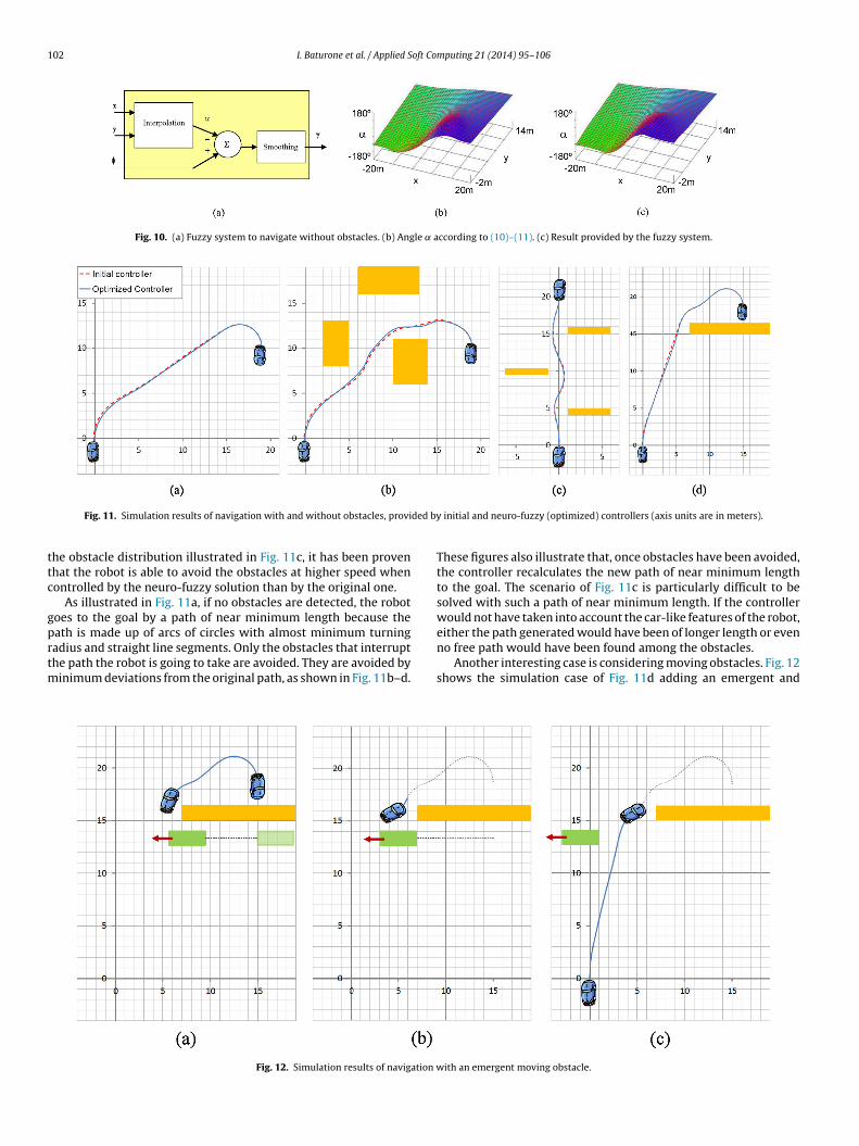

102 I. Baturone et al. / Applied Soft Computing 21 (2014) 95–106

Fig. 10. (a) Fuzzy system to navigate without obstacles. (b) Angle according to (10)–(11). (c) Result provided by the fuzzy system.

ded by

ttc

gprtm

Fig. 11. Simulation results of navigation with and without obstacles, provi

he obstacle distribution illustrated in Fig. 11c, it has been provenhat the robot is able to avoid the obstacles at higher speed whenontrolled by the neuro-fuzzy solution than by the original one.

As illustrated in Fig. 11a, if no obstacles are detected, the robotoes to the goal by a path of near minimum length because the

ath is made up of arcs of circles with almost minimum turningadius and straight line segments. Only the obstacles that interrupthe path the robot is going to take are avoided. They are avoided by

inimum deviations from the original path, as shown in Fig. 11b–d.

Fig. 12. Simulation results of navigation w

initial and neuro-fuzzy (optimized) controllers (axis units are in meters).

These figures also illustrate that, once obstacles have been avoided,the controller recalculates the new path of near minimum lengthto the goal. The scenario of Fig. 11c is particularly difficult to besolved with such a path of near minimum length. If the controllerwould not have taken into account the car-like features of the robot,

either the path generated would have been of longer length or evenno free path would have been found among the obstacles.

Another interesting case is considering moving obstacles. Fig. 12shows the simulation case of Fig. 11d adding an emergent and

ith an emergent moving obstacle.

I. Baturone et al. / Applied Soft Computing 21 (2014) 95–106 103

cles o

mttart

tpatTIraerccids

pnTrttwFwrFFvaaFaF

cations. In the system designed, MicroBlaze processor includes afloating point unit so as to carry out Eqs. (1)–(11). A timer is added asperipheral in order to evaluate the number of clock cycles investedby the processor in the four main modules of the control algorithm:

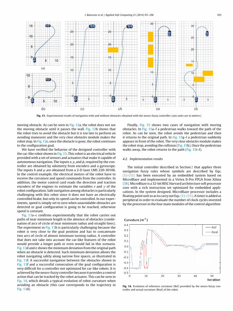
Fig. 13. Experimental results of navigation with and without obsta

oving obstacle. As can be seen in Fig. 12a, the robot does not seehe moving obstacle until it passes the wall. Fig. 12b shows thathe robot tries to avoid the obstacle but it is too late to perform anvoiding maneuver and the very close obstacles module makes theobot stop. In Fig. 12c, once the obstacle is gone, the robot continueso the configuration goal.

We have verified the behavior of the designed controller withhe car-like robot shown in Fig. 15. This robot is an electrical vehiclerovided with a set of sensors and actuators that make it capable ofutonomous navigation. The inputs x, y, and �, required by the con-roller are obtained by odometry from encoders and a gyroscope.he inputs h and ϕ are obtained from a 2-D laser LMS 220-30106.n the control example, the electrical motors of the robot have toeceive the curvature and speed commands from the controller. Inddition, the motor control card reads the direction and tractionncoders of the engines to estimate the variables v and � of theobot configuration. Safe navigation among obstacles is particularlyhallenging with this robot since it does not have an electricallyontrolled brake, but only its speed can be controlled. In our exper-ments, speed is simply set to zero when unavoidable obstacles areetected or goal configuration is going to be reached, otherwisepeed is constant.

Fig. 13a–c confirms experimentally that the robot carries outaths of near minimum length in the absence of obstacles (combi-ation of arcs of circle of near minimum radius and straight lines).he experiment in Fig. 13b is particularly challenging because theobot is very close to the goal position and has to concatenatewo arcs of circle of almost minimum turning radius. A controllerhat does not take into account the car-like features of the robotould provide a longer path or even would fail in this scenario.

ig. 13d and e shows the minimum deviation from the original pathhen an obstacle is detected. Such minimum deviation allows the

obot navigating safely along narrow free spaces, as illustrated inig. 13f. A successful navigation between the obstacles shown inig. 13f and a successful consecution of the goal configuration isery difficult for a controller not optimized for car-like robots. It ischieved by the neuro-fuzzy controller because it provides a control

ction that can be tracked by the robot actuator. This can be seen inig. 14, which details a typical evolution of robot curvature whenvoiding an obstacle (this case corresponds to the trajectory inig. 13d).

btained with the neuro-fuzzy controller (axis units are in meters).

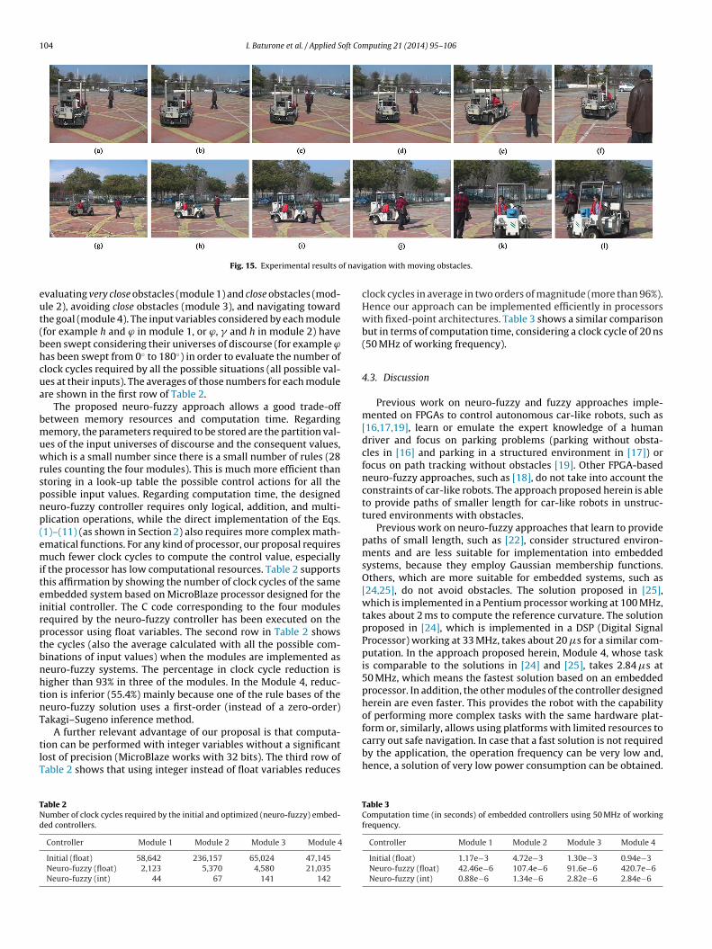
Finally, Fig. 15 shows two cases of navigation with movingobstacles. In Fig. 15a–f a pedestrian walks toward the path of therobot. As can be seen, the robot avoids the pedestrian and thenit returns to the original path. In Fig. 15g–l a pedestrian suddenlyappears in front of the robot. The very close obstacles module makesthe robot stop, avoiding the collision (Fig. 15h). Once the pedestrianwalks away, the robot returns to the path (Fig. 15i–l).

4.2. Implementation results

The initial controller described in Section 2 that applies threenavigation fuzzy rules whose symbols are described by Eqs.(1)–(11) has been executed by an embedded system based onMicroBlaze and implemented in a Virtex II-Pro FPGA from Xilinx[38]. MicroBlaze is a 32-bit RISC Harvard architecture soft processorcore with a rich instruction set optimized for embedded appli-

Fig. 14. Evolution of reference curvature (Ref) provided by the neuro-fuzzy con-troller and actual curvature (Real) of the robot.

104 I. Baturone et al. / Applied Soft Computing 21 (2014) 95–106

f navi

eut(bhcua

bmuwrspnp(emiteirptbnhtnT

tlT

TNd

Fig. 15. Experimental results o

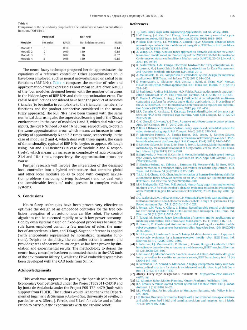
valuating very close obstacles (module 1) and close obstacles (mod-le 2), avoiding close obstacles (module 3), and navigating towardhe goal (module 4). The input variables considered by each modulefor example h and ϕ in module 1, or ϕ, � and h in module 2) haveeen swept considering their universes of discourse (for example ϕas been swept from 0◦ to 180◦) in order to evaluate the number oflock cycles required by all the possible situations (all possible val-es at their inputs). The averages of those numbers for each modulere shown in the first row of Table 2.

The proposed neuro-fuzzy approach allows a good trade-offetween memory resources and computation time. Regardingemory, the parameters required to be stored are the partition val-

es of the input universes of discourse and the consequent values,hich is a small number since there is a small number of rules (28

ules counting the four modules). This is much more efficient thantoring in a look-up table the possible control actions for all theossible input values. Regarding computation time, the designedeuro-fuzzy controller requires only logical, addition, and multi-lication operations, while the direct implementation of the Eqs.1)–(11) (as shown in Section 2) also requires more complex math-matical functions. For any kind of processor, our proposal requiresuch fewer clock cycles to compute the control value, especially

f the processor has low computational resources. Table 2 supportshis affirmation by showing the number of clock cycles of the samembedded system based on MicroBlaze processor designed for thenitial controller. The C code corresponding to the four modulesequired by the neuro-fuzzy controller has been executed on therocessor using float variables. The second row in Table 2 showshe cycles (also the average calculated with all the possible com-inations of input values) when the modules are implemented aseuro-fuzzy systems. The percentage in clock cycle reduction isigher than 93% in three of the modules. In the Module 4, reduc-ion is inferior (55.4%) mainly because one of the rule bases of theeuro-fuzzy solution uses a first-order (instead of a zero-order)akagi–Sugeno inference method.

A further relevant advantage of our proposal is that computa-

ion can be performed with integer variables without a significantost of precision (MicroBlaze works with 32 bits). The third row ofable 2 shows that using integer instead of float variables reduces

able 2umber of clock cycles required by the initial and optimized (neuro-fuzzy) embed-ed controllers.

Controller Module 1 Module 2 Module 3 Module 4

Initial (float) 58,642 236,157 65,024 47,145Neuro-fuzzy (float) 2,123 5,370 4,580 21,035Neuro-fuzzy (int) 44 67 141 142

gation with moving obstacles.

clock cycles in average in two orders of magnitude (more than 96%).Hence our approach can be implemented efficiently in processorswith fixed-point architectures. Table 3 shows a similar comparisonbut in terms of computation time, considering a clock cycle of 20 ns(50 MHz of working frequency).

4.3. Discussion

Previous work on neuro-fuzzy and fuzzy approaches imple-mented on FPGAs to control autonomous car-like robots, such as[16,17,19], learn or emulate the expert knowledge of a humandriver and focus on parking problems (parking without obsta-cles in [16] and parking in a structured environment in [17]) orfocus on path tracking without obstacles [19]. Other FPGA-basedneuro-fuzzy approaches, such as [18], do not take into account theconstraints of car-like robots. The approach proposed herein is ableto provide paths of smaller length for car-like robots in unstruc-tured environments with obstacles.

Previous work on neuro-fuzzy approaches that learn to providepaths of small length, such as [22], consider structured environ-ments and are less suitable for implementation into embeddedsystems, because they employ Gaussian membership functions.Others, which are more suitable for embedded systems, such as[24,25], do not avoid obstacles. The solution proposed in [25],which is implemented in a Pentium processor working at 100 MHz,takes about 2 ms to compute the reference curvature. The solutionproposed in [24], which is implemented in a DSP (Digital SignalProcessor) working at 33 MHz, takes about 20 �s for a similar com-putation. In the approach proposed herein, Module 4, whose taskis comparable to the solutions in [24] and [25], takes 2.84 �s at50 MHz, which means the fastest solution based on an embeddedprocessor. In addition, the other modules of the controller designedherein are even faster. This provides the robot with the capabilityof performing more complex tasks with the same hardware plat-form or, similarly, allows using platforms with limited resources to

carry out safe navigation. In case that a fast solution is not requiredby the application, the operation frequency can be very low and,hence, a solution of very low power consumption can be obtained.

Table 3Computation time (in seconds) of embedded controllers using 50 MHz of workingfrequency.

Controller Module 1 Module 2 Module 3 Module 4

Initial (float) 1.17e−3 4.72e−3 1.30e−3 0.94e−3Neuro-fuzzy (float) 42.46e−6 107.4e−6 91.6e−6 420.7e−6Neuro-fuzzy (int) 0.88e−6 1.34e−6 2.82e−6 2.84e−6

I. Baturone et al. / Applied Soft Co

Table 4Comparison of the neuro-fuzzy proposal with neural networks based on radial basisfunctions (RBF NNs).

Proposal RBF NNs

Module No. rules RMSE No. hidden neurons RMSE

Module 1 5 0.14 30 0.14

ehfaoirtffneitpcout2w

latts

5

olatrb(tpunob

A

Ebsmpr

[

[

[

[

[

[

[

[

[

[

[

[

[

[

[

[

[

[

[[

Module 2 7 0.09 150 0.15Module 3 5 0.07 16 0.07Module 4 11 0.08 180 0.15

The neuro-fuzzy technique proposed herein approximates thequations of a reference controller. Other approximators couldave been employed, such as neural networks based on radial basis

unctions (RBF NNs). Table 4 compares the number of rules andpproximation error (expressed as root mean square error, RMSE)f the four modules designed herein with the number of neuronsn the hidden layer of RBF NNs and their approximation error. Theadial basis functions considered have been the product of isoscelesriangles (to be similar in complexity to the triangular membershipunctions and the product connective considered in the neuro-uzzy approach). The RBF NNs have been trained with the sameumerical data, using also the supervised learning tool of the Xfuzzynvironment. In the case of modules 1 and 3, which deal with twonputs, the RBF NNs need 30 and 16 neurons, respectively, to obtainhe same approximation error, which means an increase in com-lexity of approximately 6 and 3.2 times more, respectively. In thease of modules 2 and 4, which deal with three inputs, the cursef dimensionality, typical of RBF NNs, begins to appear. Althoughsing 150 and 180 neurons (in case of module 2 and 4, respec-ively), which means an increase in complexity of approximately1.4 and 16.4 times, respectively, the approximation errors areorse.

Further research will involve the integration of the designedocal controller into a hybrid architecture that contains globalnd other local modules so as to cope with complex naviga-ion problems (including driving backward) and to deal withhe considerable levels of noise present in complex roboticystems.

. Conclusions

Neuro-fuzzy techniques have been proven very effective toptimize the design of an embedded controller for the free col-ision navigation of an autonomous car-like robot. The controllgorithm can be executed rapidly or with low power consump-ion by even systems based on fixed-point processors because theule bases employed contain a few number of rules, the num-er of antecedents is low, and Takagi–Sugeno inference is appliedwith antecedents represented by normalized triangular func-ions). Despite its simplicity, the controller action is smooth androvides paths of near minimum length, as has been proven by sim-lation and experimental results. The methodology to design theeuro-fuzzy controller has been automated thanks to the CAD toolsf the environment Xfuzzy 3, while the FPGA embedded system haseen developed with the CAD tools from Xilinx.

cknowledgements

This work was supported in part by the Spanish Ministerio deconomía y Competitividad under the Project TEC2011-24319 andy Junta de Andalucía under the Project P09-TEP-4479 (both with

upport from FEDER). The authors would like to thank the Depart-ent of Ingeniería de Sistemas y Automática, University of Seville, in

articular to A. Ollero, J. Ferruz, and F. Leal for advice and collabo-ation to carry out the experiments with the car-like robot.

[

[

mputing 21 (2014) 95–106 105

References

[1] T.J. Ross, Fuzzy Logic with Engineering Applications, 3rd ed., Wiley, 2010.[2] H.-P. Huang, J.-L. Yan, T.-H. Cheng, Development and fuzzy control of a pipe

inspection robot, IEEE Trans. Ind. Electron. 57 (3) (2010) 1088–1095.[3] P. Rusu, E.M. Petriu, T.E. Whalen, A. Cornell, H.J.W. Spoelder, Behavior-based

neuro-fuzzy controller for mobile robot navigation, IEEE Trans. Instrum. Meas.52 (4) (2003) 1335–1340.

[4] X. Wang, S.X. Yang, A neuro-fuzzy approach to obstacle avoidance for a non-holonomic mobile robot, in: Proceedings of the 2003 IEEE/ASME InternationalConference on Advanced Intelligent Mechatronics (AIM’03), 20–24 July, vol. 1,2003, pp. 29–34.

[5] K. Basterretxea, I. del Campo, Electronic hardware for fuzzy computation, in:A. Laurent, M.-J. Lesot (Eds.), Scalable Fuzzy Algorithms for Data Managementand Analysis: Methods and Design, IGI Global, 2010.

[6] A. Malinowski, H. Yu, Comparison of embedded system design for industrialapplications, IEEE Trans. Ind. Inform. 7 (2) (2011) 244–254.

[7] E. Monmasson, L. Idkhajine, M.N. Cirstea, I. Bahri, A. Tisan, M.W. Naouar,FPGAs in industrial control applications, IEEE Trans. Ind. Inform. 7 (2) (2011)224–243.

[8] J.J. Rodriguez-Andina, M.J. Moure, M.D. Valdes, Features, design tools and appli-cation domains of FPGAs, IEEE Trans. Ind. Electron. 54 (4) (2007) 1810–1823.

[9] D. Majoe, L. Widmer, L. Ling, J. Kao, J. Gutknecht, A reconfigurable multi-corecomputing platform for robotics and e-Health applications, in: Proceedings ofthe 2012 IEEE/ACIS 11th International Conference on Computer and Informa-tion Science (ICIS’12), 30 May–1 June, 2012, pp. 451–456.

10] M.A. Cavuslu, C. Karakuzu, F. Karakaya, Neural identification of dynamic sys-tems on FPGA with improved PSO learning, Appl. Soft Comput. 12 (9) (2012)2707–2718.

11] C.-Y. Chen, R.-C. Hwang, Y.-J. Chen, A passive auto-focus camera control system,Appl. Soft Comput. 10 (1) (2010) 296–303.

12] P. Brox, I. Baturone, S. Sánchez-Solano, Fuzzy logic-based embedded system forvideo de-interlacing, Appl. Soft Comput. 14 (C) (2014) 338–346.

13] F. Montesino-Pouzols, A. Barriga-Barros, D.R. López, S. Sánchez-Solano,Enabling fuzzy technologies in high performance networking via an open FPGA-based development platform, Appl. Soft Comput. 12 (4) (2012) 1440–1450.

14] S. Sánchez-Solano, M. Brox, E. del Toro, P. Brox, I. Baturone, Model-based designmethodology for rapid development of fuzzy controllers on FPGAs, IEEE Trans.Ind. Inform. 9 (3) (2013) 1361–1370.

15] R. Sepúlveda, O. Montiel, O. Castillo, P. Melin, Embedding a high speed intervaltype-2 fuzzy controller for a real plant into an FPGA, Appl. Soft Comput. 12 (3)(2012) 988–998.

16] S. Sánchez-Solano, A.J. Cabrera, I. Baturone, F.J. Moreno-Velo, M. Brox, FPGAimplementation of embedded fuzzy controllers for robotic applications, IEEETrans. Ind. Electron. 54 (4) (2007) 1937–1945.

17] T.S. Li, S.-J. Chang, Y.-X. Chen, Implementation of human-like driving skills byautonomous fuzzy behavior control on an FPGA-based car-like mobile robot,IEEE Trans. Ind. Electron. 50 (5) (2003) 867–880.

18] M.N. Mahyuddin, C.Z. Wei, M.R. Arshad, Neuro-fuzzy algorithm implementedin Altera’s FPGA for mobile robot’s obstacle avoidance mission, in: Proceedingsof the 2009 IEEE Region 10 Conference (TENCON’09), 23–26 January, 2009, pp.1–6.

19] S.G. Tzafestas, K.M. Deliparaschos, G.P. Moustris, Fuzzy logic path tracking con-trol for autonomous non-holonomic mobile robots: design of System on a Chip,Robot. Autonom. Syst. 58 (8) (2010) 1017–1027.

20] J. Ferruz, V.M. Vega, A. Ollero, V. Blanco, Reconfigurable control architecturefor distributed systems in the HERO autonomous helicopter, IEEE Trans. Ind.Electron. 58 (12) (2011) 5311–5318.

21] T. Takagi, M. Sugeno, Fuzzy identification of systems and its applications tomodeling and control, IEEE Trans. Syst. Man Cybern. 15 (1) (1985) 116–132.

22] K. Demirli, M. Khoshnejad, Autonomous parallel parking of a car-like mobilerobot by a neuro-fuzzy sensor-based controller, Fuzzy Sets Syst. 160 (19) (2009)2876–2891.

23] N. Uchiyama, T. Hashimo, S. Sano, S. Takagi, Model-reference control approachto obstacle avoidance for a human-operated mobile robot, IEEE Trans. Ind.Electron. 56 (10) (2009) 3892–3896.

24] I. Baturone, F.J. Moreno-Velo, V. Blanco, J. Ferruz, Design of embedded DSP-based fuzzy controllers for autonomous mobile robots, IEEE Trans. Ind. Electron.55 (2) (2008) 928–936.

25] I. Baturone, F.J. Moreno-Velo, S. Sánchez-Solano, A. Ollero, Automatic design offuzzy controllers for car-like autonomous robots, IEEE Trans. Fuzzy Syst. 12 (4)(2004) 447–465.

26] K. Samsudin, F.A. Ahmad, S. Mashohor, A highly interpretable fuzzy rule baseusing ordinal structure for obstacle avoidance of mobile robot, Appl. Soft Com-put. 11 (2) (2011) 1631–1637.

27] Xfuzzy. Fuzzy logic design tools. Available at: http://www.imse-cnm.csic.es/Xfuzzy

28] J.C. Latombe, Robot Motion Planning, Kluwer Academic Publishers, 1991.29] R.A. Brooks, A robust layered control system for a mobile robot, IEEE J. Robot.

Automat. 2 (1) (1986) 14–23.30] M.J. Wooldridge, An Introduction to Multiagent Systems, John Wiley & Sons

Ltd, 2009.31] L.E. Dubins, On curves of minimal length with a constraint on average curvature

and with prescribed initial and terminal positions and tangents, Am. J. Math.79 (3) (1957) 497–516.

1 oft Co

[

[

[

[

[

06 I. Baturone et al. / Applied S

32] J.A. Reeds, R.A. Shepp, Optimal path for a car that goes both forward and back-ward, Pac. J. Math. 145 (2) (1990) 367–393.

33] G. Desaulniers, On shortest paths for a car-like robot maneuvering around

obstacles, Robot. Autonom. Syst. 17 (3) (1996) 139–148.

34] N. Ghita, M. Kloetzer, Trajectory planning for a car-like robot by environmentabstraction, Robot. Autonom. Syst. 60 (4) (2012) 609–619.

35] R. Battiti, First- and second-order methods for learning: between steepestdescent and Newton’s method, Neural Comput. 4 (2) (1992) 141–166.

[

[

mputing 21 (2014) 95–106

36] F.J. Moreno-Velo, I. Baturone, A. Barriga, S. Sánchez-Solano, Automatic tuningof complex fuzzy systems with Xfuzzy, Fuzzy Sets Syst. 158 (18) (2007)2026–2038.

37] I. Baturone, F.J. Moreno-Velo, A. Gersnoviez, A CAD approach to simplifyfuzzy system description, in: Proceedings of the 2006 IEEE Interna-tional Conference on Fuzzy Systems (FUZZ-IEEE’06), 16–21 July, 2006,pp. 2392–2399.

38] Virtex-II Pro and Virtex-II Pro X FPGA User Guide, Xilinx, 2007.