New Optimization Methods for Modern Machine Learningsjakkamr/papers/proposal.pdf · Modern Machine Learning ... veloping convex models and algorithms ... problems by developing optimization

November 9, 2016DRAFT

New Optimization Methods for ModernMachine Learning

Sashank J. Reddi

November 2016

School of Computer ScienceCarnegie Mellon University

Pittsburgh, PA 15213

Thesis Committee:Alexander J. Smola, Co-Chair

Barnabas Poczos, Co-chairGeoffery J. Gordon

Suvrit Sra (Massachussetts Institute of Technology)Stephen Boyd (Stanford University)

Submitted in partial fulfillment of the requirementsfor the degree of Doctor of Philosophy.

Copyright c© 2016 Sashank J. Reddi


Keywords: machine learning, optimization, large-scale, distributed


AbstractModern Machine Learning (ML) systems pose several new statistical, scalability,

privacy and ethical challenges. This thesis focuses on important challenges related toscalability, such as computational and communication efficiency, often encounteredwhile solving ML problems in large-scale distributed settings.

The first part of the thesis investigates new optimization methods for solvinglarge-scale nonconvex finite-sum problems, typically referred to as empirical riskminimization (ERM) in ML. Traditionally, most of the focus in ML has been on de-veloping convex models and algorithms (e.g., SVM and logistic regression). How-ever, recently, nonconvex models have surged into limelight (notably via deep learn-ing) and have led to exciting progress — for instance these models have completelyrevolutionized areas like computer vision and natural language processing. But ourunderstanding of optimization methods suitable for these problems is still very lim-ited. Driven by this limitation, we develop and analyze a new line of optimizationmethods for nonconvex ERM problems aimed at resolving important open problemsin the wider stochastic optimization literature. For example, we develop noncon-vex stochastic methods that enjoy provably faster convergence (to stationary points)than SGD and its deterministic counterpart, gradient descent, thereby marking thefirst theoretical improvement in this line of research. We also discuss surprisingchallenges in nonsmooth and constrained nonconvex ERM problems and present afew preliminary results addressing them. Finally, we show that the key principlesbehind our methods are generalizable and can be used to overcome challenges inother important problems such as Bayesian posterior inference.

The second part of the thesis studies two critical aspects of modern distributedML systems — asynchronicity and communication efficiency of optimization meth-ods. In the context of asynchronous optimization, we study various asynchronous al-gorithms with fast convergence for finite-sum optimization problems and show thatthese methods achieve near linear speedups in sparse settings common to ML. Inaddition to asynchronicity, communication efficiency also plays an important role indetermining the overall performance of the system. However, traditional optimiza-tion algorithms used in ML are often ill-suited for distributed environments withhigh communication cost. To address this issue, we discuss two different paradigmsto achieve communication efficiency of algorithms in distributed environments andexplore new algorithms with better communication complexity.


iv


Chapter 1

Introduction

Machine learning (ML) and intelligent systems have become an indispensable part of our modernsociety. These systems are now used for variety of tasks that includes search engine, recommen-dation engines, self-driving cars and autonomous robots. Most of these systems rely on recog-nizing patterns in observable data in order to understand the data or make new predictions on theunseen data. The advent of modern data collection methods and increased computing machineryhave fueled the development of such ML systems. However, modern ML applications also posenew challenges in terms of scalability and efficiency, privacy and ethics; thus, addressing themis critical to the development of the field. This thesis is a step in the direction of addressing thesenew challenges in modern ML applications.

We start our discussion by further explaining the goals of this thesis. Modern machine learn-ing applications are heavily rooted in statistics and typically involve two major tasks: (i) con-structing a model that generates the observable data. (ii) learn the parameters of the model usingthe observable data. This thesis particularly focuses on developing fast and efficient mathemati-cal optimization methods to address problem (ii) in modern ML applications. For the purpose ofour discussion, consider the classical problem of classification using a logistic regression clas-sifier. The samples (zi, yi)ni=1 where zi ∈ Rd and yi ∈ −1, 1 for all i ∈ [n] forms thedataset where zi is referred to as features and yi the corresponding class label. In this case, theoptimization problem of our interest is:

minx∈Rd

1

n

n∑i=1

log(1 + exp(−yiz>i x)) +1

2‖x‖2. (1.1)

The term log(1+exp(−yiz>i x)) represents the loss with respect to the ith sample. The term ‖x‖2,referred to as regularization, improves the quality of the solution by providing better generaliza-tion over unseen data. One of the most interesting aspect of this problem is that it is separableover sample data points. Statistically speaking, such an attribute results from the assumptionthat the sample points are i.i.d from a probability distribution. In modern ML applications,the number of data points n is very large, in which case exploiting the separable nature of theoptimization problem becomes important. More generally, in most part of this thesis, we are

1


interested in solving optimization problems of the following form:

minx∈X

1

n

n∑i=1

fi(x) + r(x), (1.2)

where X is a compact convex set. Optimization problems of this form, typically referred to asempirical risk minimization (ERM) problems or finite-sum problems, are central to most appli-cations in ML. For example, in logistic regression problem, fi(x) = log(1 + exp(−yiz>i x)),r(x) = 1

2‖x‖2 and X = Rd. In general, for supervised learning tasks, x, fi and r represent the

parameter of our interest, loss with respect to ith data point and regularization respectively. Inmost instances, a closed-form solution for problems of form 1.2 does not exist. Hence, one hasto resort to numerical optimization techniques in order to obtain a solution. Numerical optimiza-tion methods based on first-order methods (i.e., based on gradient information of the function)are particularly favored in ML community due to their scalable nature. Popular methods includegradient descent, stochastic gradient descent and randomized coordinate descent. However, aswill see later, these methods can be significantly improved by further exploiting the structure ofthe problem in (1.2).

Before proceeding any further, one needs to understand the characteristics and requirementsof modern machine learning applications in order to appreciate the contributions of this work.Modern ML applications have added the following two new dimensions to the traditional ones.

1. Increased complexity of the model. Traditionally, most of the focus in machine learninghas been on developing convex models and algorithms (e.g., SVM, logistic regression).However, recently, nonconvex models have surged into the limelight (notably via deeplearning) and led to exciting progress – for instance these models have provided state-of-the-art performance and have completely revolutionized areas like computer vision, naturallanguage processing. Thus, developing fast and principled optimization techniques forsolving these complex models becomes important.

2. Large-scale and distributed data. With the advent of modern data collection methods,the size of the datasets used in ML applications have increased tremendously. Thus, thedataset is huge and distributed across several computing nodes. For example, large scaledistributed machine learning systems such as the Parameter server [25], GraphLab [63]and TensorFlow [1] work with datasets sizes in the order of hundreds of terabytes. Whendealing with datasets of such scale in distributed systems, computational and communica-tion workloads need to be designed carefully.

The main focus of this thesis is to make the progress geared towards addressing these importantaspects of the modern machine learning applications. Traditionally, for small-scale nonconvexoptimization problems of form (1.2) that arise in ML, batch gradient methods have been used.However, in the large-scale setting i.e., n is very large in (1.2), batch methods become in-tractable. In such scenarios, the popular stochastic gradient method (SGD) proposed by Robbinsand Monro [54] is often preferred. SGD is an iterative first-order method wherein each step ittakes a step in the negative direction of the stochastic approximation of the gradient. However,one of the fundamental issues with SGD is the noise due to the stochastic approximation of thegradient slows the convergence of the algorithm. In order to control the noise in the gradient,one has to typically decrease the step size as the algorithm proceeds. This in turn leads to slow

2


convergence and furthermore, raises the question of selection of step size and its decreasing rate.For the first part of the thesis, we address this problem in the context of nonconvex optimizationproblems by developing optimization algorithms with provable guarantees and faster conver-gence rates. Furthermore, we prove various interesting properties of these algorithms. Thesealgorithms are based on the variance reduction techniques recently developed in the context ofconvex optimization [21, 56, 58]. Furthermore, we will investigate different scenarios includingnon-smoothness of the objective function and constrained minimization problems.

For the second part of my thesis, we look into the problem of asynchronous and distributedempirical risk minimization problems. In particular, we assume a setting where parallelism isimportant and communication between the nodes is expensive. In order to meet these require-ments, the distributed optimization algorithm needs to be robust in terms of (i) synchronicity and(ii) the communication load of the overall system. To address the first part, we propose asyn-chronous stochastic algorithms with linear convergence guarantees when the objective functionin (1.2) for strongly-convex. To our knowledge, this is the first work showing asynchronoussystem with linear convergence guarantees for strongly-convex objectives. These results alsoextend to the non-strongly convex case. More details of the results will be provided in Chapter 3.As mentioned earlier, another important constraint on the distributed optimization algorithm isthe overall communication load on the system. To tackle this issue, we propose two differentparadigms for minimizing the communication complexity of the distributed algorithm. We dis-cuss and provide a few preliminary results on the performance of the algorithms in Chapter 3.

1.1 Overview of the Proposal FormatIn this chapter, I provided a high level overview of my research that forms of the core of thisthesis. In Chapters 2 and 3, I will discuss more details of the my research in addressing the twoimportant issues raised in these chapters and provide details of the work that is planned to beincorporated in the thesis. Chapter 4 briefly summarizes my other research contributions that arenot included in my thesis.

Approximate Timeline• Date of Proposal: 16th November, 2016.• Chapter 1 (Proposed work): Spring and Summer, 2017.• Chapter 2 (Proposed work): Fall, 2017.

3


4


Chapter 2

Beyond Convexity: Fast OptimizationMethods for Nonconvex Finite-sumProblems

In this chapter, we investigate fast stochastic methods for non-convex finite-sum problems. Inparticular, we study nonconvex finite-sum problems of the form

minx∈Rd

f(x) :=1

n

n∑i=1

fi(x), (2.1)

where neither f nor the individual fi (i ∈ [n]) are necessarily convex; just Lipschitz smooth(i.e., Lipschitz continuous gradients). Problems of this form arise naturally in ML in the formof empirical risk minimization (ERM). We use Fn to denote all functions of the form (2.1).We optimize such functions in the Incremental First-order Oracle (IFO) framework [2] definedbelow.Definition 2.0.1 For f ∈ Fn, an IFO takes an index i ∈ [n] and a point x ∈ Rd, and returns thepair (fi(x),∇fi(x)).IFO based complexity analysis was introduced to study lower bounds for finite-sum problems.Algorithms that use IFOs are favored in large-scale applications as they require only a smallamount first-order information at each iteration. Two fundamental models in machine learningthat profit from IFO algorithms are (i) empirical risk minimization, which typically uses convexfinite-sum models; and (ii) deep learning, which uses nonconvex ones.

The prototypical IFO algorithm, stochastic gradient descent (SGD)1 has witnessed tremen-dous progress in the recent years. By now a variety of accelerated, parallel, and faster convergingversions are known. Among these, of particular importance are variance reduced (VR) stochasticmethods [9, 21, 56], which have delivered exciting progress such as linear convergence rates (forstrongly convex functions) as opposed to sublinear rates of ordinary SGD [35, 54]. Similar (butnot same) benefits of VR methods can also be seen in smooth convex functions. The SVRG algo-

1We use ‘incremental gradient’ and ‘stochastic gradient’ interchangeably, though we are only interested in finite-sum problems.

5


Algorithm Nonconvex Convex Gradient Dominated Fixed Step Size?

SGD O(1/ε2

)O(1/ε2

)O(1/ε2

)×

GRADIENTDESCENT O (n/ε) O (n/ε) O (nτ log(1/ε))√

SVRG O(n+ (n2/3/ε)

)O(n+ (

√n/ε)

)O((n+ n2/3τ) log(1/ε)

) √

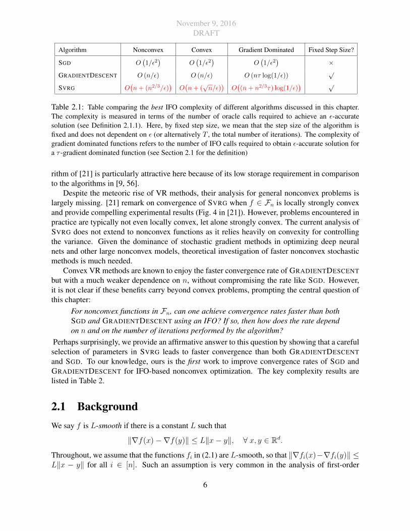
Table 2.1: Table comparing the best IFO complexity of different algorithms discussed in this chapter.The complexity is measured in terms of the number of oracle calls required to achieve an ε-accuratesolution (see Definition 2.1.1). Here, by fixed step size, we mean that the step size of the algorithm isfixed and does not dependent on ε (or alternatively T , the total number of iterations). The complexity ofgradient dominated functions refers to the number of IFO calls required to obtain ε-accurate solution fora τ -gradient dominated function (see Section 2.1 for the definition)

rithm of [21] is particularly attractive here because of its low storage requirement in comparisonto the algorithms in [9, 56].

Despite the meteoric rise of VR methods, their analysis for general nonconvex problems islargely missing. [21] remark on convergence of SVRG when f ∈ Fn is locally strongly convexand provide compelling experimental results (Fig. 4 in [21]). However, problems encountered inpractice are typically not even locally convex, let alone strongly convex. The current analysis ofSVRG does not extend to nonconvex functions as it relies heavily on convexity for controllingthe variance. Given the dominance of stochastic gradient methods in optimizing deep neuralnets and other large nonconvex models, theoretical investigation of faster nonconvex stochasticmethods is much needed.

Convex VR methods are known to enjoy the faster convergence rate of GRADIENTDESCENT

but with a much weaker dependence on n, without compromising the rate like SGD. However,it is not clear if these benefits carry beyond convex problems, prompting the central question ofthis chapter:

For nonconvex functions in Fn, can one achieve convergence rates faster than bothSGD and GRADIENTDESCENT using an IFO? If so, then how does the rate dependon n and on the number of iterations performed by the algorithm?

Perhaps surprisingly, we provide an affirmative answer to this question by showing that a carefulselection of parameters in SVRG leads to faster convergence than both GRADIENTDESCENT

and SGD. To our knowledge, ours is the first work to improve convergence rates of SGD andGRADIENTDESCENT for IFO-based nonconvex optimization. The key complexity results arelisted in Table 2.

2.1 BackgroundWe say f is L-smooth if there is a constant L such that

‖∇f(x)−∇f(y)‖ ≤ L‖x− y‖, ∀ x, y ∈ Rd.

Throughout, we assume that the functions fi in (2.1) are L-smooth, so that ‖∇fi(x)−∇fi(y)‖ ≤L‖x − y‖ for all i ∈ [n]. Such an assumption is very common in the analysis of first-order

6


methods. A function f is called λ-strongly convex if there is λ ≥ 0 such that

f(x) ≥ f(y) + 〈∇f(y), x− y〉+ λ2‖x− y‖2 ∀x, y ∈ Rd.

The quantity κ := L/λ is called the condition number of f , whenever f is L-smooth and λ-strongly convex. We say f is non-strongly convex when f is 0-strongly convex.

We also recall the class of gradient dominated functions [39, 42], where a function f is calledτ -gradient dominated if for any x ∈ Rd

f(x)− f(x∗) ≤ τ‖∇f(x)‖2, (2.2)

where x∗ is a global minimizer of f . Note that such a function f need not be convex; it is alsoeasy to show that a λ-strongly convex function is 1/2λ-gradient dominated.

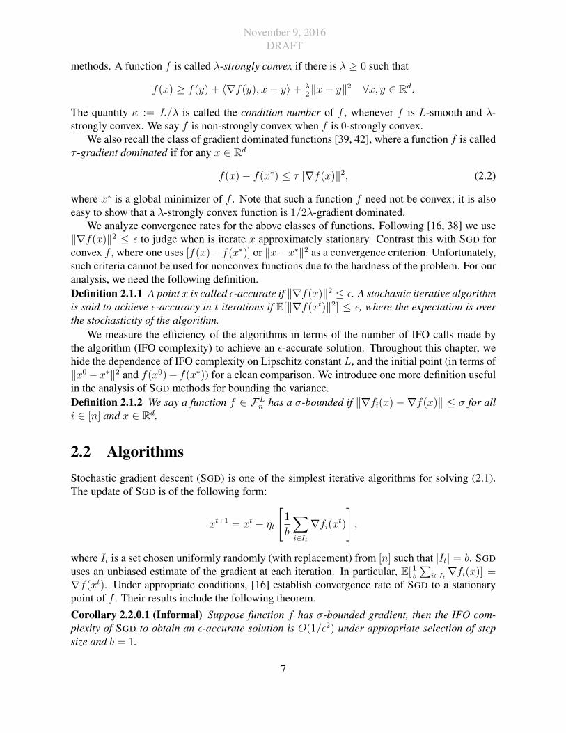
We analyze convergence rates for the above classes of functions. Following [16, 38] we use‖∇f(x)‖2 ≤ ε to judge when is iterate x approximately stationary. Contrast this with SGD forconvex f , where one uses [f(x)−f(x∗)] or ‖x−x∗‖2 as a convergence criterion. Unfortunately,such criteria cannot be used for nonconvex functions due to the hardness of the problem. For ouranalysis, we need the following definition.Definition 2.1.1 A point x is called ε-accurate if ‖∇f(x)‖2 ≤ ε. A stochastic iterative algorithmis said to achieve ε-accuracy in t iterations if E[‖∇f(xt)‖2] ≤ ε, where the expectation is overthe stochasticity of the algorithm.

We measure the efficiency of the algorithms in terms of the number of IFO calls made bythe algorithm (IFO complexity) to achieve an ε-accurate solution. Throughout this chapter, wehide the dependence of IFO complexity on Lipschitz constant L, and the initial point (in terms of‖x0− x∗‖2 and f(x0)− f(x∗)) for a clean comparison. We introduce one more definition usefulin the analysis of SGD methods for bounding the variance.Definition 2.1.2 We say a function f ∈ FLn has a σ-bounded if ‖∇fi(x) −∇f(x)‖ ≤ σ for alli ∈ [n] and x ∈ Rd.

2.2 AlgorithmsStochastic gradient descent (SGD) is one of the simplest iterative algorithms for solving (2.1).The update of SGD is of the following form:

xt+1 = xt − ηt

[1

b

∑i∈It

∇fi(xt)

],

where It is a set chosen uniformly randomly (with replacement) from [n] such that |It| = b. SGD

uses an unbiased estimate of the gradient at each iteration. In particular, E[1b

∑i∈It ∇fi(x)] =

∇f(xt). Under appropriate conditions, [16] establish convergence rate of SGD to a stationarypoint of f . Their results include the following theorem.

Corollary 2.2.0.1 (Informal) Suppose function f has σ-bounded gradient, then the IFO com-plexity of SGD to obtain an ε-accurate solution is O(1/ε2) under appropriate selection of stepsize and b = 1.

7


Algorithm 1: SVRG(x0, T,m, pimi=0, b)

1: Input: x0 = x0m = x0 ∈ Rd, epoch length m, step sizes ηi > 0m−1

i=0 , S = dT/me, discreteprobability distribution pimi=0, mini-batch size b

2: for s = 0 to S − 1 do3: xs+1

0 = xsm4: gs+1 = 1

n

∑ni=1∇fi(xs)

5: for t = 0 to m− 1 do6: Choose a mini-batch (uniformly random with replacement) It ⊂ [n] of size b7: vs+1

t = 1b

∑it∈It(∇fit(x

s+1t )−∇fit(xs)) + gs+1

8: xs+1t+1 = xs+1

t − ηtvs+1t

9: end for10: xs+1 =

∑mi=0 pix

s+1i

11: end for12: Output: Iterate xa chosen uniformly random from xs+1

t m−1t=0 Ss=0.

As seen in Corollary 2.2.0.1, SGD has a convergence rate of O(1/√T ). This rate is not improv-

able in general even when the function is (non-strongly) convex in the pure stochastic setting [36].This barrier is due to the variance introduced by the stochasticity of the gradients, and it is notclear if better rates can be obtained SGD even for (non-strongly) convex f ∈ Fn.

2.2.1 Nonconvex SVRG Algorithm

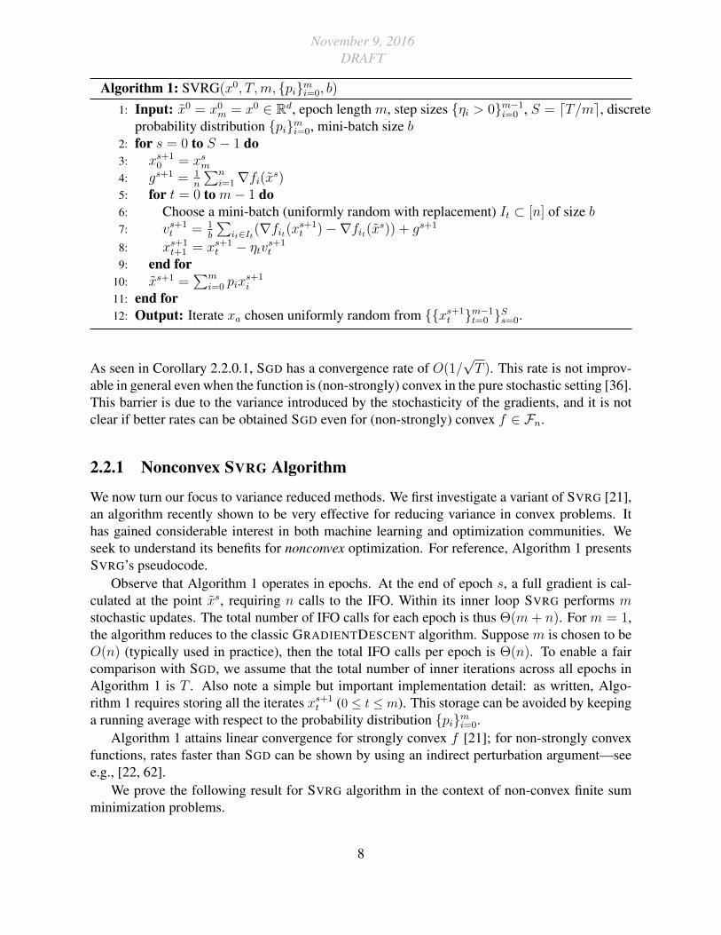
We now turn our focus to variance reduced methods. We first investigate a variant of SVRG [21],an algorithm recently shown to be very effective for reducing variance in convex problems. Ithas gained considerable interest in both machine learning and optimization communities. Weseek to understand its benefits for nonconvex optimization. For reference, Algorithm 1 presentsSVRG’s pseudocode.

Observe that Algorithm 1 operates in epochs. At the end of epoch s, a full gradient is cal-culated at the point xs, requiring n calls to the IFO. Within its inner loop SVRG performs mstochastic updates. The total number of IFO calls for each epoch is thus Θ(m + n). For m = 1,the algorithm reduces to the classic GRADIENTDESCENT algorithm. Suppose m is chosen to beO(n) (typically used in practice), then the total IFO calls per epoch is Θ(n). To enable a faircomparison with SGD, we assume that the total number of inner iterations across all epochs inAlgorithm 1 is T . Also note a simple but important implementation detail: as written, Algo-rithm 1 requires storing all the iterates xs+1

t (0 ≤ t ≤ m). This storage can be avoided by keepinga running average with respect to the probability distribution pimi=0.

Algorithm 1 attains linear convergence for strongly convex f [21]; for non-strongly convexfunctions, rates faster than SGD can be shown by using an indirect perturbation argument—seee.g., [22, 62].

We prove the following result for SVRG algorithm in the context of non-convex finite summinimization problems.

8


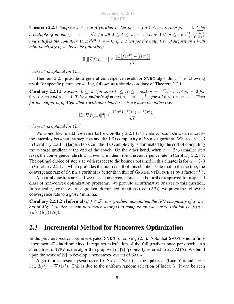
Theorem 2.2.1 Suppose b ≤ n in Algorithm 1. Let pi = 0 for 0 ≤ i < m and pm = 1, T be

a multiple of m and ηt = η = ρ/L for all 0 ≤ t ≤ m − 1, where 0 < ρ ≤ min14,√

b3m

and satisfies the condition 144m2ρ3 ≤ b + 6mρ2. Then for the output xa of Algorithm 1 withmini-batch size b, we have the following:

E[‖∇f(xa)‖2] ≤ 8L[f(x0)− f(x∗)]

ρT,

where x∗ is optimal for (2.1).

Theorem 2.2.1 provides a general convergence result for SVRG algorithm. The followingresult for specific parameter setting, follows as a simple corollary of Theorem 2.2.1.

Corollary 2.2.1.1 Suppose b ≤ nα for some 0 ≤ α ≤ 1 and m = bn3α/2

2bc. Let pi = 0 for

0 ≤ i < m and pm = 1, T be a multiple of m and ηt = η = b4Lnα

for all 0 ≤ t ≤ m − 1. Thenfor the output xa of Algorithm 1 with mini-batch size b, we have the following:

E[‖∇f(xa)‖2] ≤ 32nαL[f(x0)− f(x∗)]

bT,

where x∗ is optimal for (2.1).

We would like to add few remarks for Corollary 2.2.1.1. The above result shows an interest-ing interplay between the step size and the IFO complexity of SVRG algorithm. When α ≤ 2/3in Corollary 2.2.1.1 (larger step size), the IFO complexity is dominated by the cost of computingthe average gradient at the end of the epoch. On the other hand, when α > 2/3 (smaller stepsize), the convergence rate slows down, as evident from the convergence rate in Corollary 2.2.1.1.The optimal choice of step size with respect to the bounds obtained in this chapter is for α = 2/3in Corollary 2.2.1.1, which provides the main result of this chapter. Note that in this setting, theconvergence rate of SVRG algorithm is better than that of GRADIENTDESCENT by a factor n1/3.

A natural question arises if we these convergence rates can be further improved for a specialclass of non-convex optimization problems. We provide an affirmative answer to this question.In particular, for the class of gradient dominated functions (see (2.2)), we prove the followingconvergence rate to a global minima.

Corollary 2.2.1.2 (Informal) If f ∈ Fn is τ -gradient dominated, the IFO complexity of a vari-ant of Alg. 1 (under certain parameter settings) to compute an ε-accurate solution is O((n +τn2/3) log(1/ε)).

2.3 Incremental Method for Nonconvex OptimizationIn the previous section, we investigated SVRG for solving (2.1). Note that SVRG is not a fully“incremental” algorithm since it requires calculation of the full gradient once per epoch. Analternative to SVRG is the algorithm proposed in [9] (popularly referred to as SAGA). We buildupon the work of [9] to develop a nonconvex variant of SAGA.

Algorithm 2 presents pseudocode for SAGA. Note that the update vt (Line 5) is unbiased,i.e., E[vt] = ∇f(xt). This is due to the uniform random selection of index it. It can be seen

9


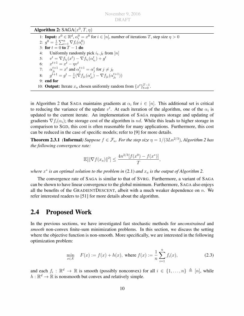
Algorithm 2: SAGA(x0, T, η)

1: Input: x0 ∈ Rd, α0i = x0 for i ∈ [n], number of iterations T , step size η > 0

2: g0 = 1n

∑ni=1∇fi(α0

i )3: for t = 0 to T − 1 do4: Uniformly randomly pick it, jt from [n]5: vt = ∇fit(xt)−∇fit(αtit) + gt

6: xt+1 = xt − ηvt7: αt+1

jt= xt and αt+1

j = αtj for j 6= jt

8: gt+1 = gt − 1n(∇fjt(α

tjt)−∇fjt(αt+1

jt))

9: end for10: Output: Iterate xa chosen uniformly random from xtT−1

t=0 .

in Algorithm 2 that SAGA maintains gradients at αi for i ∈ [n]. This additional set is criticalto reducing the variance of the update vt. At each iteration of the algorithm, one of the αi isupdated to the current iterate. An implementation of SAGA requires storage and updating ofgradients ∇fi(αi); the storage cost of the algorithm is nd. While this leads to higher storage incomparison to SGD, this cost is often reasonable for many applications. Furthermore, this costcan be reduced in the case of specific models; refer to [9] for more details.

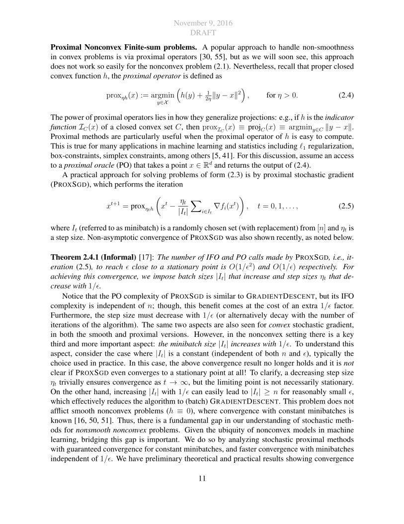
Theorem 2.3.1 (Informal) Suppose f ∈ Fn. For the step size η = 1/(3Ln2/3), Algorithm 2 hasthe following convergence rate:

E[‖∇f(xa)‖2] ≤ 4n2/3[f(x0)− f(x∗)]

T,

where x∗ is an optimal solution to the problem in (2.1) and xa is the output of Algorithm 2.

The convergence rate of SAGA is similar to that of SVRG. Furthermore, a variant of SAGA

can be shown to have linear convergence to the global minimum. Furthermore, SAGA also enjoysall the benefits of the GRADIENTDESCENT, albeit with a much weaker dependence on n. Werefer interested readers to [51] for more details about the algorithm.

2.4 Proposed WorkIn the previous sections, we have investigated fast stochastic methods for unconstrained andsmooth non-convex finite-sum minimization problems. In this section, we discuss the settingwhere the objective function is non-smooth. More specifically, we are interested in the followingoptimization problem:

minx∈X

F (x) := f(x) + h(x), where f(x) :=1

n

n∑i=1

fi(x), (2.3)

and each fi : Rd → R is smooth (possibly nonconvex) for all i ∈ 1, . . . , n , [n], whileh : Rd → R is nonsmooth but convex and relatively simple.

10


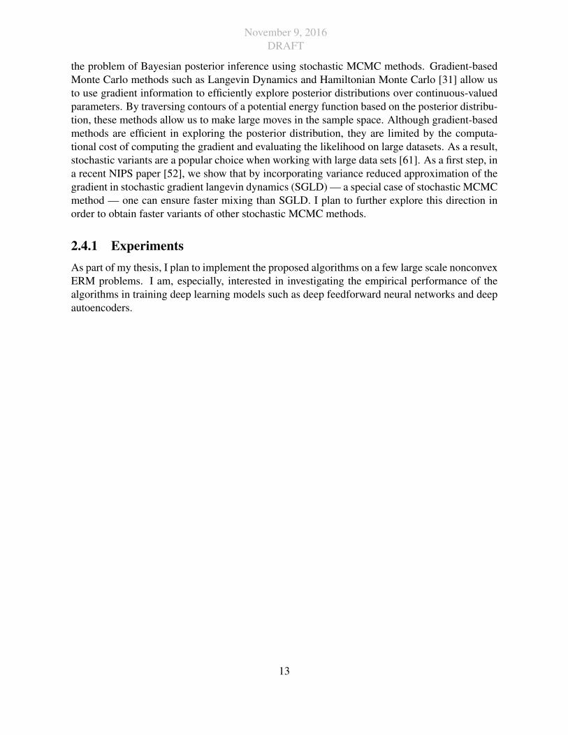
Proximal Nonconvex Finite-sum problems. A popular approach to handle non-smoothnessin convex problems is via proximal operators [30, 55], but as we will soon see, this approachdoes not work so easily for the nonconvex problem (2.1). Nevertheless, recall that proper closedconvex function h, the proximal operator is defined as

proxηh(x) := argminy∈X

(h(y) + 1

2η‖y − x‖2

), for η > 0. (2.4)

The power of proximal operators lies in how they generalize projections: e.g., if h is the indicatorfunction IC(x) of a closed convex set C, then proxIC (x) ≡ projC(x) ≡ argminy∈C ‖y − x‖.Proximal methods are particularly useful when the proximal operator of h is easy to compute.This is true for many applications in machine learning and statistics including `1 regularization,box-constraints, simplex constraints, among others [5, 41]. For this discussion, assume an accessto a proximal oracle (PO) that takes a point x ∈ Rd and returns the output of (2.4).

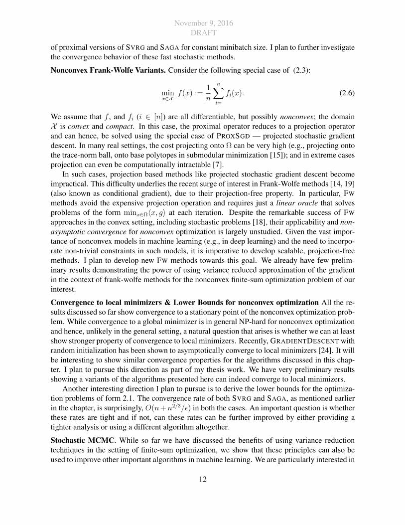
A practical approach for solving problems of form (2.3) is by proximal stochastic gradient(PROXSGD), which performs the iteration

xt+1 = proxηth

(xt − ηt

|It|∑

i∈It∇fi(xt)

), t = 0, 1, . . . , (2.5)

where It (referred to as minibatch) is a randomly chosen set (with replacement) from [n] and ηt isa step size. Non-asymptotic convergence of PROXSGD was also shown recently, as noted below.

Theorem 2.4.1 (Informal) [17]: The number of IFO and PO calls made by PROXSGD, i.e., it-eration (2.5), to reach ε close to a stationary point is O(1/ε2) and O(1/ε) respectively. Forachieving this convergence, we impose batch sizes |It| that increase and step sizes ηt that de-crease with 1/ε.

Notice that the PO complexity of PROXSGD is similar to GRADIENTDESCENT, but its IFOcomplexity is independent of n; though, this benefit comes at the cost of an extra 1/ε factor.Furthermore, the step size must decrease with 1/ε (or alternatively decay with the number ofiterations of the algorithm). The same two aspects are also seen for convex stochastic gradient,in both the smooth and proximal versions. However, in the nonconvex setting there is a keythird and more important aspect: the minibatch size |It| increases with 1/ε. To understand thisaspect, consider the case where |It| is a constant (independent of both n and ε), typically thechoice used in practice. In this case, the above convergence result no longer holds and it is notclear if PROXSGD even converges to a stationary point at all! To clarify, a decreasing step sizeηt trivially ensures convergence as t → ∞, but the limiting point is not necessarily stationary.On the other hand, increasing |It| with 1/ε can easily lead to |It| ≥ n for reasonably small ε,which effectively reduces the algorithm to (batch) GRADIENTDESCENT. This problem does notafflict smooth nonconvex problems (h ≡ 0), where convergence with constant minibatches isknown [16, 50, 51]. Thus, there is a fundamental gap in our understanding of stochastic meth-ods for nonsmooth nonconvex problems. Given the ubiquity of nonconvex models in machinelearning, bridging this gap is important. We do so by analyzing stochastic proximal methodswith guaranteed convergence for constant minibatches, and faster convergence with minibatchesindependent of 1/ε. We have preliminary theoretical and practical results showing convergence

11


of proximal versions of SVRG and SAGA for constant minibatch size. I plan to further investigatethe convergence behavior of these fast stochastic methods.

Nonconvex Frank-Wolfe Variants. Consider the following special case of (2.3):

minx∈X

f(x) :=1

n

n∑i=

fi(x). (2.6)

We assume that f , and fi (i ∈ [n]) are all differentiable, but possibly nonconvex; the domainX is convex and compact. In this case, the proximal operator reduces to a projection operatorand can hence, be solved using the special case of PROXSGD — projected stochastic gradientdescent. In many real settings, the cost projecting onto Ω can be very high (e.g., projecting ontothe trace-norm ball, onto base polytopes in submodular minimization [15]); and in extreme casesprojection can even be computationally intractable [7].

In such cases, projection based methods like projected stochastic gradient descent becomeimpractical. This difficulty underlies the recent surge of interest in Frank-Wolfe methods [14, 19](also known as conditional gradient), due to their projection-free property. In particular, FW

methods avoid the expensive projection operation and requires just a linear oracle that solvesproblems of the form minx∈Ω〈x, g〉 at each iteration. Despite the remarkable success of FW

approaches in the convex setting, including stochastic problems [18], their applicability and non-asymptotic convergence for nonconvex optimization is largely unstudied. Given the vast impor-tance of nonconvex models in machine learning (e.g., in deep learning) and the need to incorpo-rate non-trivial constraints in such models, it is imperative to develop scalable, projection-freemethods. I plan to develop new FW methods towards this goal. We already have few prelim-inary results demonstrating the power of using variance reduced approximation of the gradientin the context of frank-wolfe methods for the nonconvex finite-sum optimization problem of ourinterest.

Convergence to local minimizers & Lower Bounds for nonconvex optimization All the re-sults discussed so far show convergence to a stationary point of the nonconvex optimization prob-lem. While convergence to a global minimizer is in general NP-hard for nonconvex optimizationand hence, unlikely in the general setting, a natural question that arises is whether we can at leastshow stronger property of convergence to local minimizers. Recently, GRADIENTDESCENT withrandom initialization has been shown to asymptotically converge to local minimizers [24]. It willbe interesting to show similar convergence properties for the algorithms discussed in this chap-ter. I plan to pursue this direction as part of my thesis work. We have very preliminary resultsshowing a variants of the algorithms presented here can indeed converge to local minimizers.

Another interesting direction I plan to pursue is to derive the lower bounds for the optimiza-tion problems of form 2.1. The convergence rate of both SVRG and SAGA, as mentioned earlierin the chapter, is surprisingly, O(n+n2/3/ε) in both the cases. An important question is whetherthese rates are tight and if not, can these rates can be further improved by either providing atighter analysis or using a different algorithm altogether.

Stochastic MCMC. While so far we have discussed the benefits of using variance reductiontechniques in the setting of finite-sum optimization, we show that these principles can also beused to improve other important algorithms in machine learning. We are particularly interested in

12


the problem of Bayesian posterior inference using stochastic MCMC methods. Gradient-basedMonte Carlo methods such as Langevin Dynamics and Hamiltonian Monte Carlo [31] allow usto use gradient information to efficiently explore posterior distributions over continuous-valuedparameters. By traversing contours of a potential energy function based on the posterior distribu-tion, these methods allow us to make large moves in the sample space. Although gradient-basedmethods are efficient in exploring the posterior distribution, they are limited by the computa-tional cost of computing the gradient and evaluating the likelihood on large datasets. As a result,stochastic variants are a popular choice when working with large data sets [61]. As a first step, ina recent NIPS paper [52], we show that by incorporating variance reduced approximation of thegradient in stochastic gradient langevin dynamics (SGLD) — a special case of stochastic MCMCmethod — one can ensure faster mixing than SGLD. I plan to further explore this direction inorder to obtain faster variants of other stochastic MCMC methods.

2.4.1 ExperimentsAs part of my thesis, I plan to implement the proposed algorithms on a few large scale nonconvexERM problems. I am, especially, interested in investigating the empirical performance of thealgorithms in training deep learning models such as deep feedforward neural networks and deepautoencoders.

13


14


Chapter 3

Large-Scale Optimization: Asynchronousand Communication Efficient Optimizationfor Machine Learning

In this chapter, we investigate asynchronous and communication efficient optimization methodsfor problems that typically arise in machine learning. For the first part of the chapter, we restrictourselves to asynchronous optimization methods. Handling asynchronicity in optimization algo-rithms is important to modern ML because systems based on synchronous algorithms are oftenslow and do not exploit parallelism in distributed systems. We start our discussion by revisitingthe following finite-sum formulation in the previous section:

minx∈Rd

f(x) :=1

n

n∑i=1

fi(x). (3.1)

For most part of this chapter, we assume that the functions fi are convex. Although the valueof VR methods for solving optimization problems of form (3.1) have great value in general,for large-scale problems we still require parallel or distributed processing. And in this setting,asynchronous variants of SGD remain indispensable [3, 11, 26, 44, 59, 65]. Therefore, a keyquestion is how to develop asynchronous and distributed variants of finite-sum VR algorithms.We answer one part of this question by developing new asynchronous parallel stochastic gradientmethods that provably converge at a linear rate for smooth strongly convex finite-sum problems.

We make the following two core contributions: (i) a formal general framework for variancereduced stochastic methods based on discussions in [9]; and (ii) asynchronous parallel VR algo-rithms within this framework. Our general framework presents a formal unifying view of severalVR methods (e.g., it includes SAGA and SVRG as special cases) while expressing key algorith-mic and practical tradeoffs concisely. Thus, it yields a broader understanding of VR methods,which helps us obtain asynchronous parallel variants of VR methods. Under sparse-data settingscommon to machine learning problems, our parallel algorithms attain speedups that scale nearlinearly with the number of processors.

Related work. As already mentioned, our work is closest to (and generalizes) SAG [56],SAGA [9], SVRG [21] and S2GD [22], which are primal methods. Also closely related are dual

15


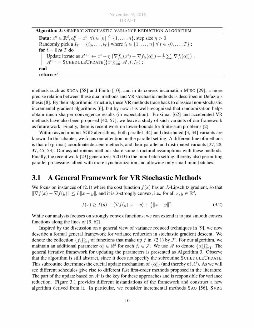
Algorithm 3: GENERIC STOCHASTIC VARIANCE REDUCTION ALGORITHM

Data: x0 ∈ Rd, α0i = x0 ∀i ∈ [n] , 1, . . . , n, step size η > 0

Randomly pick a IT = i0, . . . , iT where it ∈ 1, . . . , n ∀ t ∈ 0, . . . , T ;for t = 0 to T do

Update iterate as xt+1 ← xt − η(∇fit(xt)−∇fit(αtit) + 1

n

∑i∇fi(αti)

);

At+1 = SCHEDULEUPDATE(xit+1i=0, A

t, t, IT ) ;endreturn xT

methods such as SDCA [58] and Finito [10], and in its convex incarnation MISO [29]; a moreprecise relation between these dual methods and VR stochastic methods is described in Defazio’sthesis [8]. By their algorithmic structure, these VR methods trace back to classical non-stochasticincremental gradient algorithms [6], but by now it is well-recognized that randomization helpsobtain much sharper convergence results (in expectation). Proximal [62] and accelerated VRmethods have also been proposed [40, 57]; we leave a study of such variants of our frameworkas future work. Finally, there is recent work on lower-bounds for finite-sum problems [2].

Within asynchronous SGD algorithms, both parallel [44] and distributed [3, 34] variants areknown. In this chapter, we focus our attention on the parallel setting. A different line of methodsis that of (primal) coordinate descent methods, and their parallel and distributed variants [27, 28,37, 45, 53]. Our asynchronous methods share some structural assumptions with these methods.Finally, the recent work [23] generalizes S2GD to the mini-batch setting, thereby also permittingparallel processing, albeit with more synchronization and allowing only small mini-batches.

3.1 A General Framework for VR Stochastic MethodsWe focus on instances of (2.1) where the cost function f(x) has an L-Lipschitz gradient, so that‖∇f(x)−∇f(y)‖ ≤ L‖x− y‖, and it is λ-strongly convex, i.e., for all x, y ∈ Rd,

f(x) ≥ f(y) + 〈∇f(y), x− y〉+ λ2‖x− y‖2. (3.2)

While our analysis focuses on strongly convex functions, we can extend it to just smooth convexfunctions along the lines of [9, 62].

Inspired by the discussion on a general view of variance reduced techniques in [9], we nowdescribe a formal general framework for variance reduction in stochastic gradient descent. Wedenote the collection fini=1 of functions that make up f in (2.1) by F . For our algorithm, wemaintain an additional parameter αti ∈ Rd for each fi ∈ F . We use At to denote αtini=1. Thegeneral iterative framework for updating the parameters is presented as Algorithm 3. Observethat the algorithm is still abstract, since it does not specify the subroutine SCHEDULEUPDATE.This subroutine determines the crucial update mechanism of αti (and thereby ofAt). As we willsee different schedules give rise to different fast first-order methods proposed in the literature.The part of the update based on At is the key for these approaches and is responsible for variancereduction. Figure 3.1 provides different instantiations of the framework and construct a newalgorithm derived from it. In particular, we consider incremental methods SAG [56], SVRG

16


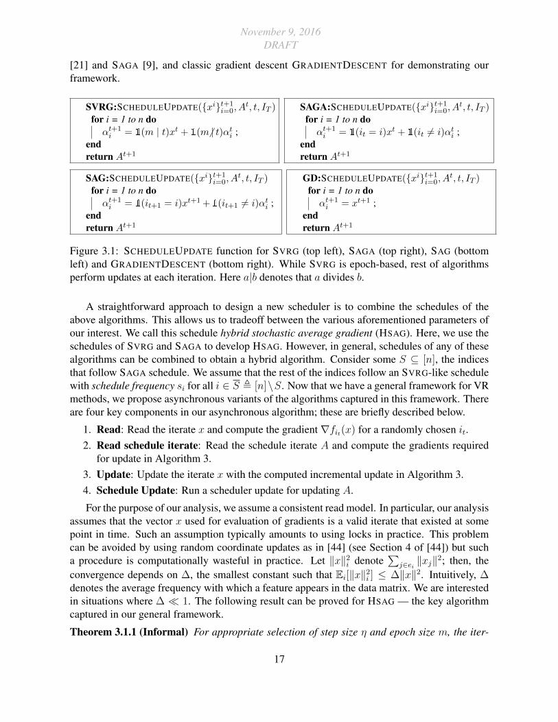
[21] and SAGA [9], and classic gradient descent GRADIENTDESCENT for demonstrating ourframework.

SVRG:SCHEDULEUPDATE(xit+1i=0, A

t, t, IT )for i = 1 to n doαt+1i = 1(m | t)xt + 1(m6 | t)αti ;

endreturn At+1

SAGA:SCHEDULEUPDATE(xit+1i=0, A

t, t, IT )for i = 1 to n doαt+1i = 1(it = i)xt + 1(it 6= i)αti ;

endreturn At+1

SAG:SCHEDULEUPDATE(xit+1i=0, A

t, t, IT )for i = 1 to n doαt+1i = 1(it+1 = i)xt+1 +1(it+1 6= i)αti ;

endreturn At+1

GD:SCHEDULEUPDATE(xit+1i=0, A

t, t, IT )for i = 1 to n doαt+1i = xt+1 ;

endreturn At+1

Figure 3.1: SCHEDULEUPDATE function for SVRG (top left), SAGA (top right), SAG (bottomleft) and GRADIENTDESCENT (bottom right). While SVRG is epoch-based, rest of algorithmsperform updates at each iteration. Here a|b denotes that a divides b.

A straightforward approach to design a new scheduler is to combine the schedules of theabove algorithms. This allows us to tradeoff between the various aforementioned parameters ofour interest. We call this schedule hybrid stochastic average gradient (HSAG). Here, we use theschedules of SVRG and SAGA to develop HSAG. However, in general, schedules of any of thesealgorithms can be combined to obtain a hybrid algorithm. Consider some S ⊆ [n], the indicesthat follow SAGA schedule. We assume that the rest of the indices follow an SVRG-like schedulewith schedule frequency si for all i ∈ S , [n]\S. Now that we have a general framework for VRmethods, we propose asynchronous variants of the algorithms captured in this framework. Thereare four key components in our asynchronous algorithm; these are briefly described below.

1. Read: Read the iterate x and compute the gradient∇fit(x) for a randomly chosen it.2. Read schedule iterate: Read the schedule iterate A and compute the gradients required

for update in Algorithm 3.3. Update: Update the iterate x with the computed incremental update in Algorithm 3.4. Schedule Update: Run a scheduler update for updating A.

For the purpose of our analysis, we assume a consistent read model. In particular, our analysisassumes that the vector x used for evaluation of gradients is a valid iterate that existed at somepoint in time. Such an assumption typically amounts to using locks in practice. This problemcan be avoided by using random coordinate updates as in [44] (see Section 4 of [44]) but sucha procedure is computationally wasteful in practice. Let ‖x‖2

i denote∑

j∈ei ‖xj‖2; then, the

convergence depends on ∆, the smallest constant such that Ei[‖x‖2i ] ≤ ∆‖x‖2. Intuitively, ∆

denotes the average frequency with which a feature appears in the data matrix. We are interestedin situations where ∆ 1. The following result can be proved for HSAG — the key algorithmcaptured in our general framework.

Theorem 3.1.1 (Informal) For appropriate selection of step size η and epoch size m, the iter-

17


ates of asynchronous variant of Algorithm 3 with HSAG schedule we have

E[f(xk)− f(x∗)

]≤ θka

[f(x0)− f(x∗)

],

where θa depends on ∆ and τ (the bound on the delay).

Under appropriate parameter settings and step size normalized by ∆1/2τ , we can show linearspeedup with τ < 1/∆1/2. Note that τ intuitively denotes the parallelism in the asynchronousalgorithm. Thus, sparsity is critical for achieving good speedups.

Randomized Coordinate Descent with Linear Constraints. We also developed asynchronousvariants for randomized coordinate descent with linear constraints. In this setting, we are inter-ested in the following composite objective convex problem with non-separable linear constraints

minxF (x) := f(x) + h(x) s.t. Ax = 0. (3.3)

Here, f : Rd → R is assumed to be continuously differentiable and convex, while h : Rd →R ∪ ∞ is lower semi-continuous, convex, coordinate-wise separable, but not necessarilysmooth; the linear constraints are specified by a matrix A ∈ Rm×d, for which m d. In a UAI2015 paper [45], we develop asynchronous randomized coordinate descent method for solvingoptimization problems of this form. The reader might wonder the connection between optimiza-tion problem (3.3) and finite-sum minimization problems of our interest. However, observe thatany finite-sum minimization problem minx

1n

∑i fi(x) can be rewritten using variable-splitting

as

minxi=x,∀i∈[N ]

1

n

N∑i=1

fi(xi).

Solving the problem in distributed environment requires considerable synchronization (for theconsensus constraint), which can slow down the algorithm significantly. However, the dual ofthe problem is

minλ

1

n

N∑i=1

f ∗i (λi) s.tN∑i=1

λi = 0,

where f ∗i is the Fenchel conjugate of fi. This reformulation perfectly fits our problem formu-lation in (3.3) and can be solved in an asynchronous manner using the procedure proposed inour paper. Other interesting application include constrained least square problem, multi-agentplanning problems, resource allocation—see [32, 33] and references therein for more examples.We refer interested readers to [45] for more details about the algorithm.

3.2 Proposed WorkCommunication Efficient Optimization Algorithms. In the previous sections of this chapter,we discussed asynchronous optimization algorithms for problems that arise in machine learn-ing. However, the communication efficiency of these algorithms was not examined. In modern

18


distributed ML systems, machines read and write global parameter frequently. This data accessrequires massive amount of network bandwidth and hence, communication efficiency of opti-mization algorithms is critical. To this end, we develop and discuss new communication efficientoptimization algorithms.

For the purpose of this discussion, we assume a parameter server architecture for investigat-ing these algorithms. Such a setup entails a server group and a worker group where each groupcontains several threads/machines. The server machines mainly serve the purpose of maintainingthe global parameters, while most of the workload needs to be allocated to the worker machines.The communication between the worker and the server group is the assumed to the main bot-tleneck and hence, needs to minimized. We plan to investigate the following two paradigms foraddress this problem in the context of ML.

1. Iterative algorithms like SGD often require large amount of communication between workerand server machines. The first approach to reduce this communication cost is by construct-ing a small summary of the training data — which acts as a proxy for the entire data set— and communicating it to the server machine; thereby, eliminating the need for frequentcommunication between the worker and the server machines. Such an approach entails (i)computing these summaries of data at the worker nodes (which can be computationallyintensive), (ii) sending these small summaries to a server machine (a low communicationoverhead task) and (iii) finally, solving a small optimization problem at the server ma-chines. This summary of the training points is called a coreset. While this methodologyhas been successfully applied to data clustering problems like k-means and k-median (werefer the reader to [12, 13] for a comprehensive survey), it remains largely unexploredfor supervised learning and optimization problems. I have a preliminary algorithm thatuses this methodology in the context of solving empirical loss minimization problems forparticular loss functions. I plan to investigate this direction further.

2. An alternate approach is to perform most of the computation at the worker machines in anembarrassingly manner and combine the solutions from all the worker machines; thereby,eliminating the need to communicate to the server machine frequently. Note that suchan operation needs to be done in an iterative fashion in order to each an optimal solutionto our optimization problem. ADMM (alternating direction method of multipliers) is anpopular approach for solving distribution optimization problems that follows this method-ology. Under certain conditions, ADMM is shown to achieve communication complexityof O(

√L/λ log(1/ε)) for L-smooth and λ-strongly convex function. More recently, the

DANE, DISCO and COCOA+ algorithms have been proposed to tackle the problem of re-ducing the communication complexity in solving problems of form (2.1) [20, 60, 64].DISCO is particularly appealing because they match communication complexity lowerbounds derived in [4]. However, DISCO requires a second-order oracle for its executionand is not embarrassingly parallel. I am working on developing a first-order algorithm thatnot only achieves the communication lower bounds in [4] but can be also be implementedin an embarrassingly parallel fashion.

19


3.2.1 ExperimentsFor my thesis, I plan to investigate the performance of the proposed algorithms on a few popularML problems, such as linear and logistic regression, for fairly large datasets. In particular, it willbe interesting to understand practical speedups and communication complexities of the proposedalgorithms on large sparse datasets.

20


Chapter 4

My Other Research — In a Nutshell

Besides optimization methods for machine learning applications, I have also worked on a numberof other topics such as kernel methods, hypothesis testing, dependence measures, functionalregression, which are not part of my thesis. Here, I briefly describe my contributions that formthe core of my research in these areas.

Kernel Methods, Dependence Measures & Hypothesis Testing. Measuring dependenciesand conditional dependencies are of great importance in many scientific fields including machinelearning, and statistics. There are numerous problems where we want to know how large thedependence is between random variables, and how this dependence changes if we observe otherrandom variables. In an ICML 2013 paper [46], we developed new kernel based dependencemeasures with scale invariance property and showed the effectiveness of our dependence measureon real-world problems. I also worked on kernel based two sample testing problem. In particular,in a series of papers [43, 48, 49] we proved (through theoretical and empirical results) that MMDbased two sample testing — a kernel based two sample test — also suffers from the curse ofdimensionality. Such a result was important because there was a wide misconception that thesemeasures do not suffer from the curse of dimensionality and hence, also work for high dimensionproblems. Our papers cleared this misconception and provided first theoretical results for thepower of the MMD based two sample hypothesis tests.

Machine Learning on Functional Data. Another important aspect of many modern ma-chine learning applications is the structure in the input data. Modern data collection techniquesmotivate settings where the training data is no longer of simple form such as features. For exam-ple, a Facebook user profile contains very rich information about the user such as posts, friendslist, likes, photos, polls, etc. Unfortunately, most of the existing machine learning and statisticaltechniques cannot handle such data, often resorting to ad-hoc approaches, thereby ignoring theunderlying rich structure in the data. This necessitates the development of a different machinelearning paradigm where the true structure in the complex data can be exploited. In a UAI’14[47], we developed a simple nearest neighbor based algorithm for handling data of various forms.In fact, we considered a strictly generalized scenario of noisy and incomplete/missing data. Weanalyzed the theoretical properties of our proposed estimator and demonstrated its performancethrough practical experiments. We also proposed an approach to choose the number of nearestneighbors to be used, thereby alleviating the problem of cross validation in nearest neighborbased algorithms.

21


22


Bibliography

[1] Martın Abadi, Ashish Agarwal, Paul Barham, Eugene Brevdo, Zhifeng Chen, Craig Citro,Greg S Corrado, Andy Davis, Jeffrey Dean, Matthieu Devin, et al. Tensorflow: Large-scalemachine learning on heterogeneous distributed systems. arXiv:1603.04467, 2016. 2

[2] A. Agarwal and L. Bottou. A lower bound for the optimization of finite sums.arXiv:1410.0723, 2014. 2, 3

[3] Alekh Agarwal and John C Duchi. Distributed delayed stochastic optimization. In Ad-vances in Neural Information Processing Systems, pages 873–881, 2011. 3

[4] Yossi Arjevani and Ohad Shamir. Communication complexity of distributed convex learn-ing and optimization. In C. Cortes, N. D. Lawrence, D. D. Lee, M. Sugiyama, and R. Gar-nett, editors, Advances in Neural Information Processing Systems 28, pages 1747–1755.2015. 2

[5] F. Bach, R. Jenatton, J. Mairal, and G. Obozinski. Convex optimization with sparsity-inducing norms. In S. Sra, S. Nowozin, and S. J. Wright, editors, Optimization for MachineLearning. MIT Press, 2011. 2.4

[6] Dimitri P Bertsekas. Incremental gradient, subgradient, and proximal methods for convexoptimization: A survey. Optimization for Machine Learning, 2010:1–38, 2011. 3

[7] Michael Collins, Amir Globerson, Terry Koo, Xavier Carreras, and Peter L Bartlett. Expo-nentiated gradient algorithms for conditional random fields and max-margin markov net-works. JMLR, 9:1775–1822, 2008. 2.4

[8] Aaron Defazio. New Optimization Methods for Machine Learning. PhD thesis, AustralianNational University, 2014. 3

[9] Aaron Defazio, Francis Bach, and Simon Lacoste-Julien. SAGA: A fast incremental gradi-ent method with support for non-strongly convex composite objectives. In NIPS 27, pages1646–1654. 2014. 2, 2.3, 3, 3.1

[10] Aaron J Defazio, Tiberio S Caetano, and Justin Domke. Finito: A faster, permutable incre-mental gradient method for big data problems. arXiv:1407.2710, 2014. 3

[11] Ofer Dekel, Ran Gilad-Bachrach, Ohad Shamir, and Lin Xiao. Optimal distributed onlineprediction using mini-batches. The Journal of Machine Learning Research, 13(1):165–202,2012. 3

[12] Dan Feldman and Michael Langberg. A unified framework for approximating and cluster-ing data. In Proceedings of the Forty-third Annual ACM Symposium on Theory of Comput-

23


ing, STOC ’11, pages 569–578, 2011. ISBN 978-1-4503-0691-1. 1

[13] Dan Feldman, Melanie Schmidt, and Christian Sohler. Turning big data into tiny data:Constant-size coresets for k-means, pca and projective clustering. In Proceedings of theTwenty-Fourth Annual ACM-SIAM Symposium on Discrete Algorithms, SODA ’13, pages1434–1453, 2013. ISBN 978-1-611972-51-1. 1

[14] Marguerite Frank and Philip Wolfe. An algorithm for quadratic programming. Naval Re-search Logistics Quarterly, 3(1-2):95–110, March 1956. 2.4

[15] Satoru Fujishige and Shigueo Isotani. A submodular function minimization algorithmbased on the minimum-norm base. Pacific Journal of Optimization, 7(1):3–17, 2011. 2.4

[16] Saeed Ghadimi and Guanghui Lan. Stochastic first- and zeroth-order methods for noncon-vex stochastic programming. SIAM Journal on Optimization, 23(4):2341–2368, 2013. doi:10.1137/120880811. 2.1, 2.2, 2.4

[17] Saeed Ghadimi, Guanghui Lan, and Hongchao Zhang. Mini-batch stochastic approxima-tion methods for nonconvex stochastic composite optimization. Mathematical Program-ming, 155(1-2):267–305, 2014. 2.4.1

[18] Elad Hazan and Haipeng Luo. Variance-reduced and projection-free stochastic optimiza-tion. CoRR, abs/1602.02101, 2016. 2.4

[19] Martin Jaggi. Revisiting Frank-Wolfe: Projection-free sparse convex optimization. InICML’13, pages 427–435, 2013. 2.4

[20] Martin Jaggi, Virginia Smith, Martin Takac, Jonathan Terhorst, Sanjay Krishnan, ThomasHofmann, and Michael I Jordan. Communication-Efficient Distributed Dual CoordinateAscent. In NIPS 27, pages 3068–3076. 2014. 2

[21] Rie Johnson and Tong Zhang. Accelerating stochastic gradient descent using predictivevariance reduction. In NIPS 26, pages 315–323. 2013. 1, 2, 2.2.1, 3, 3.1

[22] Jakub Konecny and Peter Richtarik. Semi-Stochastic Gradient Descent Methods.arXiv:1312.1666, 2013. 2.2.1, 3

[23] Jakub Konecny, Jie Liu, Peter Richtarik, and Martin Takac. Mini-Batch Semi-StochasticGradient Descent in the Proximal Setting. arXiv:1504.04407, 2015. 3

[24] Jason D. Lee, Max Simchowitz, Michael I. Jordan, and Benjamin Recht. Gradient descentonly converges to minimizers. In Proceedings of the 29th Conference on Learning Theory,COLT 2016, New York, USA, June 23-26, 2016, pages 1246–1257, 2016. 2.4

[25] Mu Li, David G Andersen, Alex J Smola, and Kai Yu. Communication efficient distributedmachine learning with the parameter server. In Z. Ghahramani, M. Welling, C. Cortes,N. D. Lawrence, and K. Q. Weinberger, editors, Advances in Neural Information ProcessingSystems 27, pages 19–27. Curran Associates, Inc., 2014. 2

[26] Mu Li, David G Andersen, Alex J Smola, and Kai Yu. Communication Efficient DistributedMachine Learning with the Parameter Server. In NIPS 27, pages 19–27, 2014. 3

[27] Ji Liu and Stephen J. Wright. Asynchronous stochastic coordinate descent: Parallelism andconvergence properties. SIAM Journal on Optimization, 25(1):351–376, 2015. 3

24


[28] Ji Liu, Steve Wright, Christopher Re, Victor Bittorf, and Srikrishna Sridhar. An asyn-chronous parallel stochastic coordinate descent algorithm. In ICML 2014, pages 469–477,2014. 3

[29] Julien Mairal. Optimization with first-order surrogate functions. arXiv:1305.3120, 2013. 3

[30] J. J. Moreau. Fonctions convexes duales et points proximaux dans un espace hilbertien. C.R. Acad. Sci. Paris Ser. A Math., 255:2897–2899, 1962. 2.4

[31] Radford Neal. Mcmc using hamiltonian dynamics. In Handbook of Markov Chain MonteCarlo, 2010. 2.4

[32] I Necoara, Y Nesterov, and F Glineur. A random coordinate descent method on large opti-mization problems with linear constraints. Technical report, Technical Report, UniversityPolitehnica Bucharest, 2011, 2011. 3.1

[33] Ion Necoara and Andrei Patrascu. A random coordinate descent algorithm for optimizationproblems with composite objective function and linear coupled constraints. Comp. Opt.and Appl., 57(2):307–337, 2014. 3.1

[34] A Nedic, Dimitri P Bertsekas, and Vivek S Borkar. Distributed asynchronous incrementalsubgradient methods. Studies in Computational Mathematics, 8:381–407, 2001. 3

[35] A. Nemirovski, A. Juditsky, G. Lan, and A. Shapiro. Robust stochastic approximationapproach to stochastic programming. SIAM Journal on Optimization, 19(4):1574–1609,2009. 2

[36] Arkadi Nemirovski and D Yudin. Problem Complexity and Method Efficiency in Optimiza-tion. John Wiley and Sons, 1983. 2.2

[37] Yu Nesterov. Efficiency of coordinate descent methods on huge-scale optimization prob-lems. SIAM Journal on Optimization, 22(2):341–362, 2012. 3

[38] Yurii Nesterov. Introductory Lectures On Convex Optimization: A Basic Course. Springer,2003. 2.1

[39] Yurii Nesterov and Boris T Polyak. Cubic regularization of newton method and its globalperformance. Mathematical Programming, 108(1):177–205, 2006. 2.1

[40] Atsushi Nitanda. Stochastic Proximal Gradient Descent with Acceleration Techniques. InNIPS 27, pages 1574–1582, 2014. 3

[41] N. Parikh and S. Boyd. Proximal algorithms. Foundations and Trends in Optimization, 1(3):127–239, 2014. ISSN 2167-3888. 2.4

[42] B.T. Polyak. Gradient methods for the minimisation of functionals. USSR ComputationalMathematics and Mathematical Physics, 3(4):864–878, January 1963. 2.1

[43] Aaditya Ramdas, Sashank J. Reddi, Barnabas Poczos, Aarti Singh, and Larry A. Wasser-man. Adaptivity and computation-statistics tradeoffs for kernel and distance based highdimensional two sample testing. CoRR, abs/1508.00655, 2015. 4

[44] Benjamin Recht, Christopher Re, Stephen Wright, and Feng Niu. Hogwild!: A Lock-FreeApproach to Parallelizing Stochastic Gradient Descent. In NIPS 24, pages 693–701, 2011.3, 3.1

25


[45] Sashank Reddi, Ahmed Hefny, Carlton Downey, Avinava Dubey, and Suvrit Sra. Large-scale randomized-coordinate descent methods with non-separable linear constraints. In UAI31, 2015. 3, 3.1

[46] Sashank J. Reddi and Barnabas Poczos. Scale invariant conditional dependence measures.In Proceedings of the 30th International Conference on Machine Learning, ICML 2013,Atlanta, GA, USA, 16-21 June 2013, pages 1355–1363, 2013. 4

[47] Sashank J. Reddi and Barnabas Poczos. k-nn regression on functional data with incompleteobservations. In Proceedings of the Thirtieth Conference on Uncertainty in Artificial Intel-ligence, UAI 2014, Quebec City, Quebec, Canada, July 23-27, 2014, pages 692–701, 2014.4

[48] Sashank J. Reddi, Aaditya Ramdas, Barnabas Poczos, Aarti Singh, and Larry A. Wasser-man. On the decreasing power of kernel and distance based nonparametric hypothesis testsin high dimensions. In Proceedings of the Twenty-Ninth AAAI Conference on ArtificialIntelligence, January 25-30, 2015, Austin, Texas, USA., pages 3571–3577, 2015. 4

[49] Sashank J. Reddi, Aaditya Ramdas, Barnabas Poczos, Aarti Singh, and Larry A. Wasser-man. On the high dimensional power of a linear-time two sample test under mean-shiftalternatives. In Proceedings of the Eighteenth International Conference on Artificial Intel-ligence and Statistics, AISTATS 2015, San Diego, California, USA, May 9-12, 2015, 2015.4

[50] Sashank J. Reddi, Ahmed Hefny, Suvrit Sra, Barnabas Poczos, and Alexander J. Smola.Stochastic variance reduction for nonconvex optimization. In Proceedings of the 33ndInternational Conference on Machine Learning, ICML 2016, New York City, NY, USA,June 19-24, 2016, pages 314–323, 2016. 2.4

[51] Sashank J. Reddi, Suvrit Sra, Barnabas Poczos, and Alexander J. Smola. Fast incrementalmethod for nonconvex optimization. CoRR, abs/1603.06159, 2016. 2.3, 2.4

[52] Sashank J. Reddi, Suvrit Sra, Barnabas Poczos, and Alexander J. Smola. Stochastic frank-wolfe methods for nonconvex optimization. In 54th Annual Allerton Conference on Com-munication, Control, and Computing, Allerton 2016, 2016. 2.4

[53] Peter Richtarik and Martin Takac. Iteration complexity of randomized block-coordinatedescent methods for minimizing a composite function. Mathematical Programming, 144(1-2):1–38, 2014. 3

[54] H. Robbins and S. Monro. A stochastic approximation method. Annals of MathematicalStatistics, 22:400–407, 1951. 1, 2

[55] R Tyrrell Rockafellar. Monotone operators and the proximal point algorithm. SIAM journalon control and optimization, 14(5):877–898, 1976. 2.4

[56] Mark W. Schmidt, Nicolas Le Roux, and Francis R. Bach. Minimizing Finite Sums withthe Stochastic Average Gradient. arXiv:1309.2388, 2013. 1, 2, 3, 3.1

[57] Shai Shalev-Shwartz and Tong Zhang. Accelerated mini-batch stochastic dual coordinateascent. In NIPS 26, pages 378–385, 2013. 3

[58] Shai Shalev-Shwartz and Tong Zhang. Stochastic dual coordinate ascent methods for reg-

26


ularized loss. The Journal of Machine Learning Research, 14(1):567–599, 2013. 1, 3

[59] Ohad Shamir and Nathan Srebro. On distributed stochastic optimization and learning. InProceedings of the 52nd Annual Allerton Conference on Communication, Control, andComputing, 2014. 3

[60] Ohad Shamir, Nathan Srebro, and Tong Zhang. Communication efficient distributed opti-mization using an approximate newton-type method. CoRR, abs/1312.7853, 2013. 2

[61] Max Welling and Yee Whye Teh. Bayesian learning via stochastic gradient Langevin dy-namics. In ICML, 2011. 2.4

[62] Lin Xiao and Tong Zhang. A proximal stochastic gradient method with progressive variancereduction. SIAM Journal on Optimization, 24(4):2057–2075, 2014. 2.2.1, 3, 3.1

[63] Aapo Kyrola Danny Bickson Carlos Guestrin Yucheng Low, Joseph Gonzalez andJoseph M. Hellerstein. Distributed GraphLab: A Framework for Machine Learning andData Mining in the Cloud. PVLDB, 2012. 2

[64] Yuchen Zhang and Xiao Lin. Disco: Distributed optimization for self-concordant empiricalloss. In Proceedings of the 32nd International Conference on Machine Learning, ICML2015, Lille, France, 6-11 July 2015, pages 362–370, 2015. 2

[65] Martin Zinkevich, Markus Weimer, Lihong Li, and Alex J Smola. Parallelized stochasticgradient descent. In NIPS, pages 2595–2603, 2010. 3

27

Documents

New Optimization Methods for Modern Machine Learningsjakkamr/papers/proposal.pdf · Modern Machine Learning ... veloping convex models and algorithms ... problems by developing optimization