New Strategies for Impervious Surface Data Development

New Strategies

for Impervious Surface Data Development

for the King County Water Quality and Water Quantity Groups Unit

Benjamin Gardner

Elizabeth Gould

Krystle Jumawan

University of Washington Professional Master’s Program in GIS

Geography 569: GIS Workshop

August 17 2012

TableofContents

I. BACKGROUND AND PROBLEM STATEMENT .......................................................................................... 1

BACKGROUND ....................................................................................................................................... 1 PROJECT GOAL ...................................................................................................................................... 5 OBJECTIVES ........................................................................................................................................... 5 EXISTING PROCESS WORKFLOW ........................................................................................................... 6 EXISTING ACTIVITY WORKFLOW ........................................................................................................... 6 PROPOSED ACTIVITY WORKFLOW ........................................................................................................ 7 INFORMATION PRODUCTS .................................................................................................................... 9 PROJECT BENEFITS .............................................................................................................................. 13

II. SYSTEM REQUIREMENTS ..................................................................................................................... 14

SOFTWARE AND NETWORKING REQUIREMENTs ............................................................................... 14 PERSONNEL AND TIME REQUIREMENTS ............................................................................................. 15 OTHER CONSIDERATIONS ................................................................................................................... 16

III. DATA ACQUISITION ............................................................................................................................ 16

DATA DESIGN ...................................................................................................................................... 16 DATA CHARACTERISTICS ..................................................................................................................... 19 DATABASES ......................................................................................................................................... 20 LOGICAL DATABASE MODEL ............................................................................................................... 20 FUTURE DATABASE DEVELOPMENT ................................................................................................... 21

IV: DATA ANALYSIS, INFORMATION PRODUCTS, AND FINDINGS ............................................................ 22

INPUT DATA ........................................................................................................................................ 22 DATA ANALYSIS ................................................................................................................................... 22 INFORMATION PRODUCTS .................................................................................................................. 25

V. FINANCIAL & STRATEGIC ANALYSIS .................................................................................................... 25

FINANCIAL ANALYSIS ........................................................................................................................... 25 STRATEGIC ANALYSIS .......................................................................................................................... 27 RECOMMENDED COURSE OF ACTION ................................................................................................. 28

VI. FUTURE DIRECTIONS .......................................................................................................................... 28

REFERENCES ............................................................................................................................................ 31

ii

List of Acronyms Used In This Document ..................................................................................... iv

APPENDICES ............................................................................................................................................ 33

APPENDIX A: ENVIRONMENT SETTINGS

APPENDIX B: WORKFLOW FOR IMPERVIOUS SURFACE EXTRACTION PROCESSES

APPENDIX C: MAPS OF IMPERVIOUS SURFACE DATA OUTPUT

APPENDIX D: DETAILED FINANCIAL AND RISK ANALYSIS

List of Figures

Figure 1: Project Location Figure 2: Organizational Structure Figure 3: Existing Process Workflow Figure 4: Existing Activity Workflow Figure 5: Proposed Activity Workflow Figure 6: Process for Creating the BHT and VHT DEM files Figure 7: Proposed Database Structure

LIST OF ACRONYMS USED IN THIS DOCUMENT

BHT Building Height

BMP Best Management Practice

CIR Color Infra‐Red

DEM Digital Elevation Model

DNRP Department of Natural Resources and Parks

EPA Environmental Protection Agency

Esri Environmental Systems Research Institute

GIS Geographic Information Systems

HSP‐F Hydrologic Simulation Program‐Fortran

KC King County

LC/LU Land Cover/Land Use

LID Low Impact Development

LiDAR Light Detection And Ranging

NPDES National Pollutant Discharge Elimination System

NVI National Vegetation Index

RAM Random Access Memory

SSWM Storm and Surface Water Management

STSS Science and Technical Support Section

SUSTAIN System for Urban Stormwater Treatment and Analysis Integration

VHT Vegetation Height

WLRD Water and Land Resources Division

WRIA Water Resource Inventory Area

WWTP Waste Water Treatment Plant

1

New Strategies for Impervious Surface Data Development

I. BACKGROUND AND PROBLEM STATEMENT

BACKGROUND

Water quality and water resource management within the Puget Sound watershed are essential for the

ecological restoration, management, and maintenance of the waters of Puget Sound. The Puget Sound

watershed includes lands in Clallam Island, Jefferson, King, Kitsap, Mason, Pierce, San Juan, Skagit,

Snohomish, Thurston, and Whatcom counties, Washington (U.S. Environmental Protection Agency

[EPA], 2012; Jim Simmonds, Science and Technical Services Section Supervisor, King County Department

of Parks and Natural Resources Water and Land Resources Division, email communication 3 July 2012).

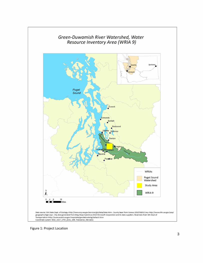
Water Resource Inventory Area (WRIA) 9, the Green/Duwamish and Central Puget Sound watershed, is

the second most populated watershed in the state. It is a source of drinking water, food, and forest

products, and is host to several species of federally Endangered Species Act salmonids, including

Chinook, Coho, chum, and steelhead and has been identified as a conservation priority. As described in

the King County (KC) Science and Technical Support Section (STSS) Business plan, stormwater is a

significant stressor affecting the health of the Puget Sound Ecosystem. Efficiently and effectively

managing stormwater to reduce harm to the ecosystem is a common goal of numerous local agencies

and actors, ranging from special interest groups to citizens and government (King County Department of

Natural Resources and Parks [KCDNRP], 2008). The KCDNRP Water and Land Resources Division (WLRD)

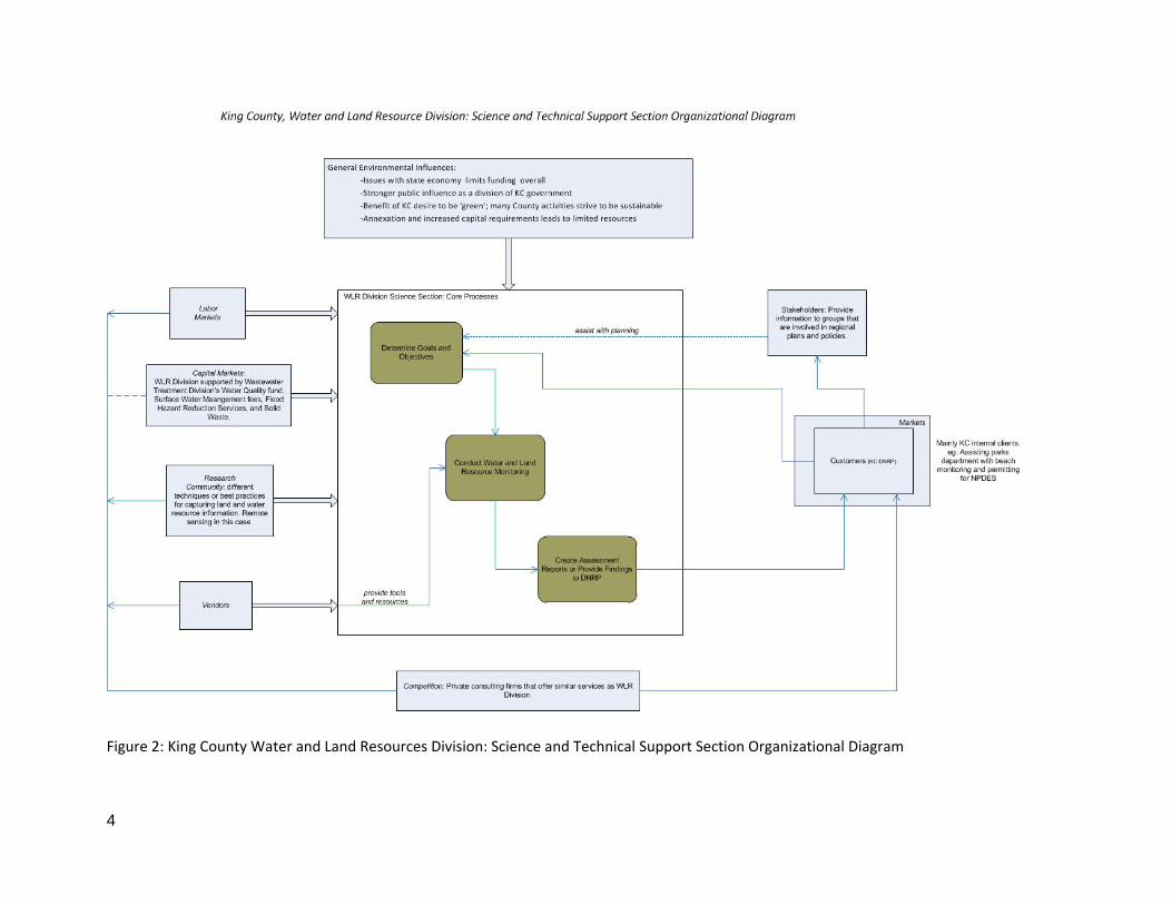
STSS exercises a critical role in this effort, as WRIA 9 lies almost entirely within the county boundary

(Figure 1), and the STSS is tasked with monitoring land and water resources, with developing and

implementing management strategies for the benefit of the resources, as well as providing information

and data for other departments to support them in their missions (Figure 2).

2

Historically, stormwater management efforts focused on concentrating and removing water from the

landscape as quickly as possible, which contributed to sediment, thermal, and contaminant impacts to

receiving waters. More recent efforts shifted to the development of regional and local systems to

manage stormwater, through a stormwater conveyance and collection infrastructure that provides a

measure of pretreatment before discharging to local waterbodies. King County is now looking forward

to the next generation of stormwater management, with a focus on developing highly localized, site

based stormwater treatment systems that provide maximum stormwater treatment benefit for the cost.

3

Figure 1: Project Location

4

Figure 2: King County Water and Land Resources Division: Science and Technical Support Section Organizational Diagram

5

PROJECT GOAL

A significant area of focus for the County and the STSS is the implementation of strategies and structures

to improve water quality via storm and surface water management (SSWM) (Jim Simmonds and Curtis

DeGasperi, meeting notes, 27 June 2012; KCDNRP, 2008). In particular, the STSS is interested in knowing

the precise locations of different types of impervious surfaces, since the type and ownership of

impervious areas affects the kinds of stormwater management features that can be used to manage the

associated runoff, and informs which approaches are most appropriate for funding and implementation.

OBJECTIVES

The objective for this project is to develop a tool that operates in Esri’s ArcGIS and which KC GIS staff

can use to automate the process of generating high resolution, fine scale, GIS‐compatible vector data

layers of land cover type from existing raster information. In other words, the county "needs to know"

the exact location and type of impervious surface in order to plan appropriate pre‐treatment strategies

for a specific site. The types of impervious surface areas to be mapped automatically include:

Commercial Parking Lots

Commercial Roofs

Industrial Parking Lots

Industrial Roofs

Multifamily Parking

Multifamily (Buildings)

Single Family Buildings

Roads

6

An area within WRIA 9 was identified as a "sample” area to test potential methodologies. This

geographic area of interest is Township 22N Range 5W‐‐the City of Covington (Figure 1)‐‐ which includes

a mixture of developed and undeveloped land cover types.

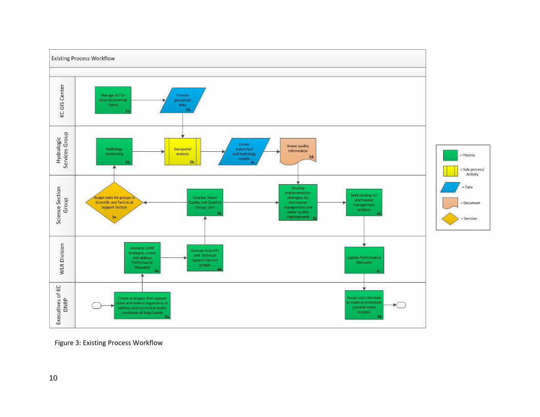
EXISTING PROCESS WORKFLOW

DNRP executives work together to create broad strategies that address environmental health conditions

of King County (Figure 3, Box 5a). (King County, 2012b) These strategies are then interpreted by the

WLRD and from these strategies performance measures are established which indicate environmental

health. WLRD is tasked with overseeing the STSS groups. Decisions must be made on how to delegate

tasks among the STSS groups, including the Hydrology section (Figure 3, Row 2). This group conducts

hydrologic monitoring and analysis to create watershed and hydrology models for KC. Hydrologic

Services works with the KC GIS Center to obtain data (Figure 3, Box 1b) to assist in hydrology modeling.

This information is then assessed and is used to develop specific strategies for conducting SSWM and

water quality improvement projects proposed by the larger STSS (Figure 3, Box 3c). To ensure that this

management is successful the STSS secure funding for projects. With the assessments made by the

Hydrologic Services group and the effectiveness of SSWM improvement projects the WLRD will update

their performance measures. This allows the DNRP to reevaluate their overarching strategies and goals

based on these indicators. If water quality conditions in King County have not improved or are

worsening then they can formulate necessary interventions (Figure 3, Box 5b).

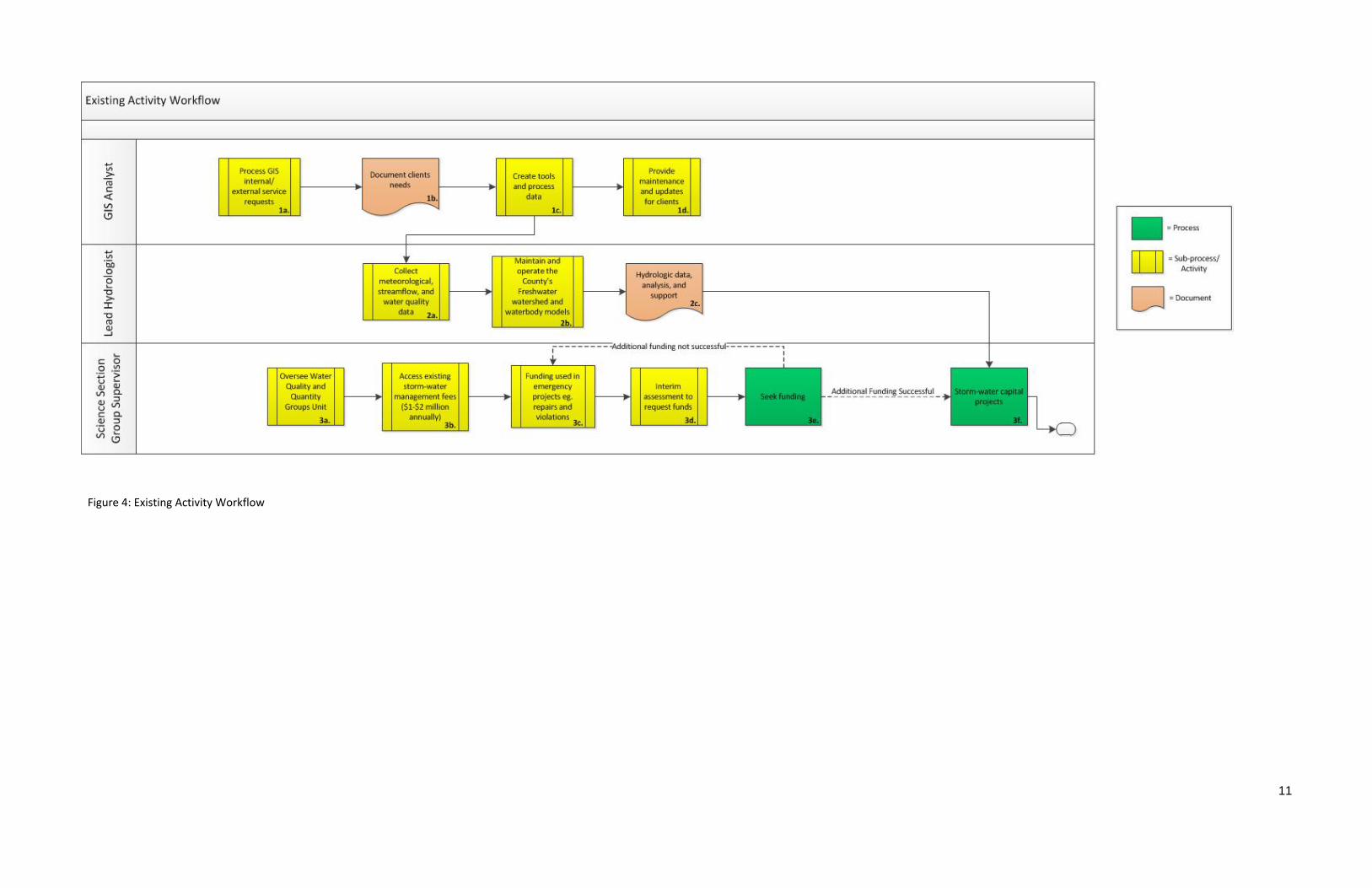
EXISTING ACTIVITY WORKFLOW

While current regulations require that the creation of new impervious surface areas include adequate

storm and surface water management treatment methods, existing or older impervious surface areas

often do not have adequate existing stormwater infrastructure. Stormwater maintenance and

improvements are currently funded via the stormwater management fee paid by KC property owners.

7

This generates $1‐2 million annually (Figure 4 Box 3b) , which is enough revenue to cover emergency

repairs to infrastructure within the stormwater management "train", and to address violations that

contribute to water quality degradation, such as erosion, but is not sufficient to cover the cost of routine

maintenance or upgrades (Figure 4, Box 3c). While KC has investigated the possibility of increasing the

fees and expanding the capital improvement program, the ten‐fold or more increase that is necessary to

fully fund needed improvements and maintenance is politically untenable, and the County remains

limited to managing only emergencies and violations. The Science section group supervisor leads this

process, with input from the lead hydrologist and data and processing support from KC GIS center

(Figure 4, Boxes 1a ‐d, 2a‐c)

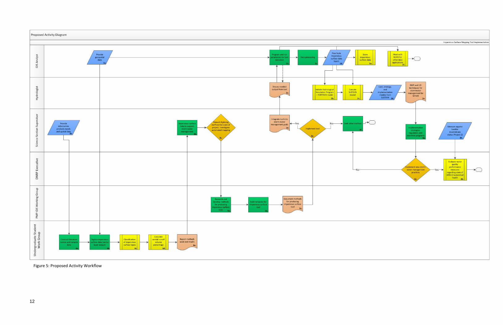
PROPOSED ACTIVITY WORKFLOW

As part of the effort to further refine King County's SSWM efforts into a highly localized treatment

system, members of the KCDNRP WLRD received EPA funding to develop models that will prioritize

areas in WRIA 9 where stormwater infrastructure installation will provide maximum benefit to water

quality (Figure 5). The modeling effort is a two‐stage process, executed by the hydrologists at KC DNRP

WLRD. The first phase (Figure 5, Box 2b) uses the Hydrologic Simulation Program‐Fortran (HSP‐F) to

develop time series data of flow and water quality at catchment pour‐points for subbasins within the

watershed. Data input into this model includes land cover, Digital Elevation Model (DEM) information,

weather, geologic information, soils, hydrologic features including stream channel morphology, incision,

and depth, and the locations and types of existing stormwater facilities (Figure 5, Box 1b). Desired

additional information to input into this model includes highly detailed information about the types and

locations of impervious surface within the model area (Figure 5, Box 1d).

8

The output from the HSPF model is then input into the EPA's SUSTAIN model (System for Urban

Stormwater Treatment and Analysis Integration) (Figure 5 Box 2c). SUSTAIN is a powerful, flexible, and

complex modeling software with the capability of outputting very specific information about the size,

types, numbers, and locations of Best Management Practices (BMPs) and Low Impact Development (LID)

strategies that will provide the maximum benefit to watershed water quality for the cost (Figure 5, Box

2a) . Once this information is available, implementation and retrofitting of the new stormwater

treatment infrastructure can be accomplished via several approaches (Figure 5 Box 3g). When existing

sites are redeveloped, permitting under the National Pollutant Discharge Elimination System (NPDES)

requires implementation of appropriate metrics and measures to eliminate discharge. For existing

properties, the ability to customize existing stormwater fees based on the site contribution may serve as

incentive for property owners to retrofit. Finally, government programs exist that can fund stormwater

management improvements on public lands; in addition to minimizing impacts arising from these lands,

stormwater treatments on these lands may be planned and designed in such a way as to treat or

mitigate from adjacent private lands (personal communications, Jim Simmonds and Victor High, meeting

11 July 2012).

However, to effectively implement this strategy, the SSTS needs to know the locations of impervious

surface at as fine a scale as possible, and to be able to distinguish the type and ownership of impervious,

as different types require different treatment strategies, and the ownership type affects which

implementation strategies are appropriate. Typically this has been accomplished via manually digitizing

vector data layers from satellite imagery (Sterr and Yui Lau, 2012). However, this process was found to

be extremely labor intensive and expensive given the geographic scope of the study area, often too

coarse in scale, and not necessarily comparable through time (Simmonds, 2012; Harmon, 2007). (Figure

5, boxes 6a‐e, Boxes 3b‐c)

9

INFORMATION PRODUCTS

The information products include fine scale vector data layers that represent the location of specific

types of impervious surface, within a 6' horizontal accuracy. Specifically, the data products include

vector layers of roof tops and pavement, organized according whether the associated land use is single

family homes, multiple‐family dwellings, commercial, or industrial. The products also include a

"blueprint" for the method for generating the data, so that KC can refine and additionally develop

outputs as needed, including potential future development of a tool to map vegetative cover type. The

method for creating the vector data layers will also be captured as a tool coded in Python and

executable within ArcGIS vers. 10.1.

10

Figure 3: Existing Process Workflow

11

Figure 4: Existing Activity Workflow

12

Figure 5: Proposed Activity Workflow

13

PROJECT BENEFITS

When developed to completion, the project will benefit water quality within WRIA 9 and Puget Sound by

allowing a very focused, directed application of stormwater management strategies within the

watershed. Because generating the data by hand is extremely labor intensive and thus very costly,

having a tool that automates the process will present a cost savings to the SSTS and KC (see Section V)

and also will make it possible to generate impervious cover data far more frequently, as well as with

greater accuracy.

While the immediate benefit of the impervious surface tool is the stormwater treatment analysis that

will be output from the SUSTAIN model, this fine scale mapping of impervious has various other

applications that will benefit water quality within the implementation area.

In addition to the funding challenges that the county faces in stormwater management, there are

practical challenges that arise naturally when working in an area with a varied and long history. One of

these is the lack of adequate information about the location ‐‐or existence‐‐of all connections between

commercial, industrial, and multifamily units and the existing stormwater infrastructure. This makes

planning and implementing maintenance of these connections impossible (Jim Simmonds, 26 July 2012).

When overlaid with the stormwater infrastructure data in GIS, the fine scale impervious data output will

facilitate the identification of locations where these connections are likely to occur.

Other challenges to water quality protection include the fact that, at the time when the City of Seattle's

original stormwater conveyance system was constructed, it was standard practice to design stormwater

systems such that any stormwater overflow resulting from heavy precipitation events was diverted to

the sanitary sewer and ultimately to the waste water treatment plants (WWTPs). This can drive up

treatment costs at the WWTP and has the potential to overwhelm the WWTP capacity, resulting in the

14

discharge of untreated water into receiving waterbodies. In some cases, cities with this design have

been able to separate the storm water and wastewater infrastructure into two different pipe systems,

however in Seattle this is both cost‐prohibitive and impractical, as it would require digging up every

street to make the necessary changes. Instead, King County and the City of Seattle are taking a two‐

pronged approach: 1. prevent stormwater from entering the system in the first place and 2. incurring

significant costs to increase the capacity of the WWTP to reduce the potential for an overflow event.

The SUSTAIN model process will allow SSTS to identify, with a much higher degree of accuracy, those

areas within the watershed that contribute a disproportionately high level of runoff into the storm

sewer system. Prioritizing these areas for stormwater rate and volume control will have significant

benefit in reducing both operations costs at WWTP during runoff events and in reducing the risk of

untreated discharge from the WWTP.

II. SYSTEM REQUIREMENTS

SOFTWARE AND NETWORKING REQUIREMENTs

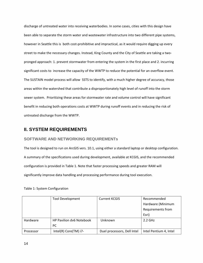
The tool is designed to run on ArcGIS vers. 10.1, using either a standard laptop or desktop configuration.

A summary of the specifications used during development, available at KCGIS, and the recommended

configuration is provided in Table 1. Note that faster processing speeds and greater RAM will

significantly improve data handling and processing performance during tool execution.

Table 1: System Configuration

Tool Development Current KCGIS Recommended

Hardware (Minimum

Requirements from

Esri)

Hardware HP Pavilion dv6 Notebook

PC

Unknown 2.2 GHz

Processor Intel(R) Core(TM) i7‐ Duel processors, Dell Intel Intel Pentium 4, Intel

15

3610QM CPU @ 2.30 GHz Xeon E5640 @2.67 GHz

and 2.66 GHz

Core Duo, or Xeon

Processors; SSE2 (or

greater)

System type 64 bit 64 bit

RAM 16.0 GB 12 GB 2GB

Operating

System

Microsoft Windows 7,

Service Pack 1

Windows 7 Professional Windows 7 Professional

Software ArcGIS version 10.1 ArcGIS version 10.1 ArcGIS version 10.1

While the tool was developed using ArcGIS vers.10.1, it may not run on earlier versions of ArcGIS, since

ArcToolbox varies among different versions of ArcGIS. However, the fundamental process outlined in

the model remains accurate.

PERSONNEL AND TIME REQUIREMENTS

Running tools in ArcGIS with larger raster data inputs can be time consuming, but once the tool is

operational, initiating execution will be straightforward. Processing the data and outputs for a 36 square

mile area takes several minutes; the processing time will increase somewhat proportionally as the study

area increases, and will be affected by variables including the complexity of land cover. In highly

developed areas, the high levels of impervious cover will require more time to process. In rural areas,

where there is less impervious, processing time may be shorter.

King County anticipates that this detailed land cover data would only need to be generated every few

years (Simmonds, 2012); the data could be updated when new LiDAR or new Land cover/Land use

(LC/LU) data becomes available, and when the county needs updated information about the detailed

location of impervious cover types. The tool is designed so that it can be executed by one person and

has the potential to be generated at a local desktop or workstation. However, the recommended "best

practice" for management and use of the tool output data is that the tool and output be maintained by

16

KCGIS, and that KC STSS staff coordinate with the KCGIS for data use; this coordination will require

minimal time.

OTHER CONSIDERATIONS

In the event of significant changes or upgrades to the ArcGIS software, it may be necessary to

implement some changes in how the tool is programmed, although the workflow process executed by

the tool will remain valid. Similarly, the impervious surface tool uses some functions and tools that are

already pre‐installed in the GIS "toolbox", and the impervious surface tool design assumes that those

pre‐installed tools are unaltered and are stored in the default location. If Esri changes where the pre‐

installed tools are stored in a future version of the software, the coding in the impervious surface tool

will need to be updated so that the sub‐processes are initiated from the correct location.

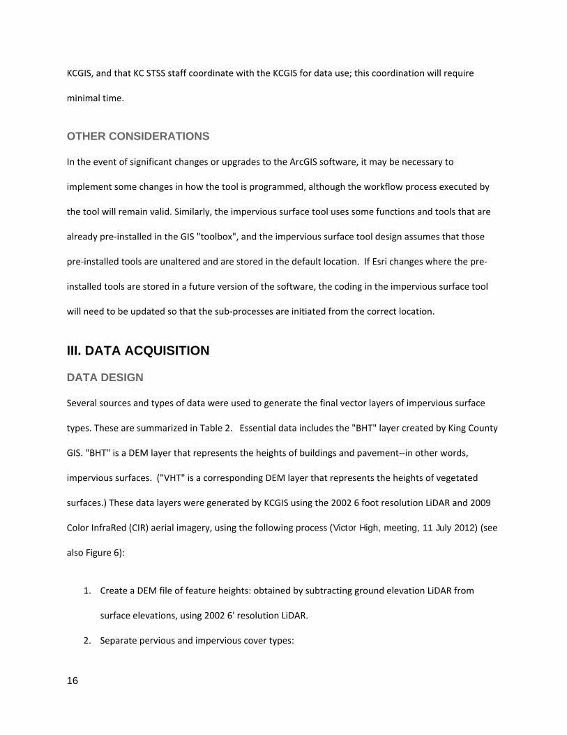
III. DATA ACQUISITION

DATA DESIGN

Several sources and types of data were used to generate the final vector layers of impervious surface

types. These are summarized in Table 2. Essential data includes the "BHT" layer created by King County

GIS. "BHT" is a DEM layer that represents the heights of buildings and pavement‐‐in other words,

impervious surfaces. ("VHT" is a corresponding DEM layer that represents the heights of vegetated

surfaces.) These data layers were generated by KCGIS using the 2002 6 foot resolution LiDAR and 2009

Color InfraRed (CIR) aerial imagery, using the following process (Victor High, meeting, 11 July 2012) (see

also Figure 6):

1. Create a DEM file of feature heights: obtained by subtracting ground elevation LiDAR from

surface elevations, using 2002 6' resolution LiDAR.

2. Separate pervious and impervious cover types:

17

(a) Create a "mask" of vegetated vs. non‐vegetated cover, using spectral signatures in the 2009

Color InfraRed (CIR) aerial photos and calculations from the National Vegetation Index (NVI)

(b) Several cover types, including water, bare earth, and recent clearcuts, will read as

"impervious" using this methodology. The King County water layer was used to subtract

water features from the impervious layer that was output in step 2a. Then, the data was

reviewed against the aerial photos and any remaining non‐impervious areas were manually

removed.

3. The resulting layer of impervious cover was used to clip the feature height LiDAR from step 1

into a "vegetation height" layer (VHT) and an "impervious height" layer (BHT).

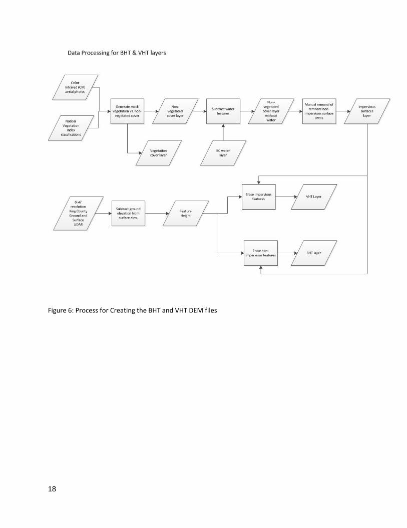
18

Figure 6: Process for Creating the BHT and VHT DEM files

19

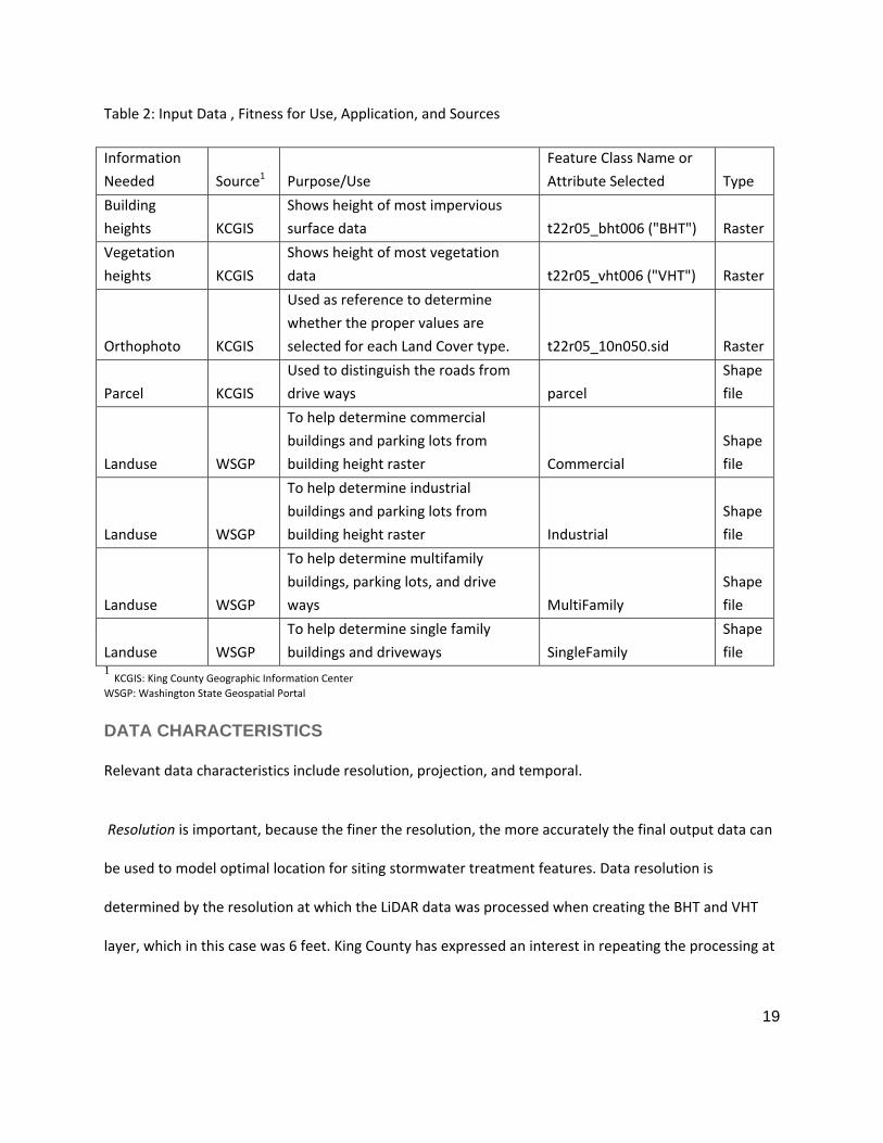
Table 2: Input Data , Fitness for Use, Application, and Sources

Information

Needed Source1 Purpose/Use

Feature Class Name or

Attribute Selected Type

Building

heights KCGIS

Shows height of most impervious

surface data t22r05_bht006 ("BHT") Raster

Vegetation

heights KCGIS

Shows height of most vegetation

data t22r05_vht006 ("VHT") Raster

Orthophoto KCGIS

Used as reference to determine

whether the proper values are

selected for each Land Cover type. t22r05_10n050.sid Raster

Parcel KCGIS

Used to distinguish the roads from

drive ways parcel

Shape

file

Landuse WSGP

To help determine commercial

buildings and parking lots from

building height raster Commercial

Shape

file

Landuse WSGP

To help determine industrial

buildings and parking lots from

building height raster Industrial

Shape

file

Landuse WSGP

To help determine multifamily

buildings, parking lots, and drive

ways MultiFamily

Shape

file

Landuse WSGP

To help determine single family

buildings and driveways SingleFamily

Shape

file 1 KCGIS: King County Geographic Information Center

WSGP: Washington State Geospatial Portal

DATA CHARACTERISTICS

Relevant data characteristics include resolution, projection, and temporal.

Resolution is important, because the finer the resolution, the more accurately the final output data can

be used to model optimal location for siting stormwater treatment features. Data resolution is

determined by the resolution at which the LiDAR data was processed when creating the BHT and VHT

layer, which in this case was 6 feet. King County has expressed an interest in repeating the processing at

20

a resolution of 3 feet at a future date. (Jim Simmonds and Victor High, personal communication, 11 July

2012).

Projection: to maintain compatibility with KCGIS data standards, data were generated in the projection

used by King County GIS: NAD_1983_StatePlane_Washington_North_FIPS_4601_Feet.

Temporal: currently, the base data (BHT and VHT data layers) reflect a "hybrid” point in time, because

the base data used to derive these files is from different time points. The LiDAR is from 2003, whereas

the Color Infrared used to separate the vegetation and impervious surfaces dates from 2009. It may be

possible to generate the fine‐scale impervious and fine‐scale land cover mapping for a particular time

point if appropriate base data becomes available.

DATABASES

The tool will operate in ArcGIS 10, running on Windows 7 Operating System, and a current version of

Microsoft Word will be used to document the metadata. The eventual data output includes raster data

and vector data (layer files). Metadata will follow KC GIS Center Metadata standards (FGDC‐1998

standards), and will be generated by KC GIS after executing the tool and creating county‐wide coverage

of the data. Tool output will also conform to KC GIS center data standards.

LOGICAL DATABASE MODEL

The database model for this project is object‐relational, which allows for integration with Esri’s ArcGIS

Object Model. This also allows for the use of relational table primary keys to provide for data

interaction, coded domains for generating data attributes, and database integrity rules. This model is

consistent with existing KC GIS protocol and standards.

21

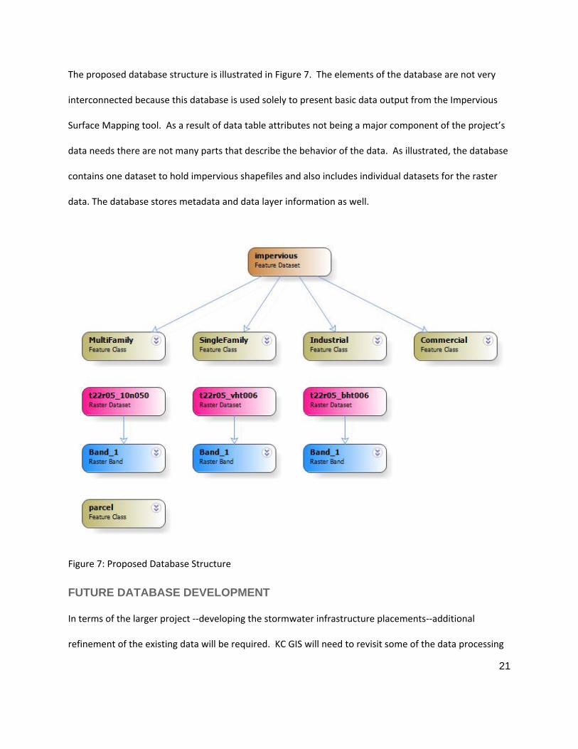
The proposed database structure is illustrated in Figure 7. The elements of the database are not very

interconnected because this database is used solely to present basic data output from the Impervious

Surface Mapping tool. As a result of data table attributes not being a major component of the project’s

data needs there are not many parts that describe the behavior of the data. As illustrated, the database

contains one dataset to hold impervious shapefiles and also includes individual datasets for the raster

data. The database stores metadata and data layer information as well.

Figure 7: Proposed Database Structure

FUTURE DATABASE DEVELOPMENT

In terms of the larger project ‐‐developing the stormwater infrastructure placements‐‐additional

refinement of the existing data will be required. KC GIS will need to revisit some of the data processing

22

steps that were conducted outside of this immediate project to develop a more refined‐‐and more

current‐ layer for BHT and VHT to capture more current conditions, and at a finer resolution.

As the larger stormwater project evolves and takes form, it may make sense for the project geodatabase

to hold additional information and attributes, according to the input needed for the stormwater model.

This will be evaluated as the project progresses.

IV: DATA ANALYSIS, INFORMATION PRODUCTS, AND FINDINGS

INPUT DATA

There are several feature layers that were input into the data processing. The first one is the "man‐

made feature height", or BHT data developed by King County GIS. This is a continuous raster data set

which stores a single value representing a general height of impervious features relative to ground

elevation. The King County parcel data and subsets of the King County land cover data were also input

(Table 2).

DATA ANALYSIS

The data analysis process involves using various layers to mask and extract different subsets of

information from the BHT file. The premise behind the analysis is to first separate building from roads

using the parcel data. The parcel data was used as the first mask, as it allowed the separation of roads,

which are not captured in the parcel layer, and driveways and parking lots, which are included in the

parcel layer. Next, the resulting output data was masked using specific subsets of the land cover data.

Finally, buildings and pavement output were distinguished based on feature height. The result is a raster

layer representing specific types of impervious cover. The last step is conversion of the raster output

into a vector data layer.

23

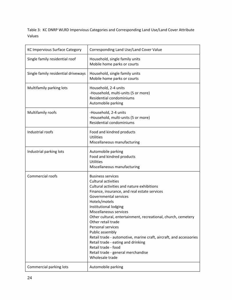
Early during the planning process, the STSS identified a number of types of impervious surface to isolate

via this tool. As part of the tool design process, these impervious surface categories were matched with

corresponding LU/LC categories as defined in the LU/LC data layer provided by KC (Table 3). The result

of this process has allowed the automated creation of raster and vector data for:

Commercial Parking Lots

Commercial Roofs

Industrial Parking Lots

Industrial Roofs

Multifamily Parking

Multifamily Roofs

Single Family Paved areas

Single Family Roofs

Roads

The full workflow for each of these processes is depicted in Appendix A. Once each vector layer has

been created, we recommend combing the separate layers into a single GIS file, and separating the

cover types within the attribute table. Since the final GIS layer will likely be posted on the KC GIS data

center, combining the layers into one file will helps ensure that end‐users have the full data set, rather

than partial data, and reduces the potential for errors of omission by subsequent users (Jim Simmonds,

meeting, 26 July 2012).

24

Table 3: KC DNRP WLRD Impervious Categories and Corresponding Land Use/Land Cover Attribute

Values

KC Impervious Surface Category Corresponding Land Use/Land Cover Value

Single family residential roof Household, single family units Mobile home parks or courts

Single family residential driveways Household, single family units Mobile home parks or courts

Multifamily parking lots Household, 2‐4 units ‐Household, multi‐units (5 or more) Residential condominiums Automobile parking

Multifamily roofs ‐Household, 2‐4 units ‐Household, multi‐units (5 or more) Residential condominiums

Industrial roofs Food and kindred products Utilities Miscellaneous manufacturing

Industrial parking lots Automobile parking Food and kindred products Utilities Miscellaneous manufacturing

Commercial roofs Business services Cultural activities Cultural activities and nature exhibitions Finance, insurance, and real estate services Governmental services Hotels/motels Institutional lodging Miscellaneous services Other cultural, entertainment, recreational, church, cemetery Other retail trade Personal services Public assembly Retail trade ‐ automotive, marine craft, aircraft, and accessoriesRetail trade ‐ eating and drinking Retail trade ‐ food Retail trade ‐ general merchandise Wholesale trade

Commercial parking lots Automobile parking

25

Business services Cultural activities Cultural activities and nature exhibitions Finance, insurance, and real estate services Governmental services Hotels/motels Institutional lodging Miscellaneous services Other cultural, entertainment, recreational, church, cemetery Other retail trade Personal services Public assembly Retail trade ‐ automotive, marine craft, aircraft, and accessoriesRetail trade ‐ eating and drinking Retail trade ‐ food Retail trade ‐ general merchandise Wholesale trade

INFORMATION PRODUCTS

There are two significant products of this project. The first is a "blueprint" for a methodology to for

automating the creation of vector impervious cover type data from existing, LiDAR derived rasters. The

second product is the data output itself. Samples of the data output for the City of Covington‐‐the study

area‐‐ are available in Appendix C.

V. FINANCIAL & STRATEGIC ANALYSIS

FINANCIAL ANALYSIS

An important consideration when evaluating whether to implement a new technology or technique is

cost: will the new approach provide a cost savings over the existing or conventional strategies? How

does the cost savings compare to the cost of implementation? To address these questions, a detailed,

step‐by‐step financial analysis was conducted (Lerner, 2007). The full analysis is presented in Appendix

D, and summarized here.

26

As outlined in the proposed activity workflow diagram (Figure 5) there are only a few positions involved

with implementing the impervious surface mapping tool: a GIS analyst, a hydrologist, and STSS

supervisor. The GIS analyst will work to integrate the tool within the King County GIS Center, and will

coordinate with the hydrologist on analysis extent and the formatting of input data prior to tool

execution. The GIS analyst will also execute the tool and assume responsibility for processing the output

data and maintaining the final dataset within the KCGIS data library. The hydrologist will work closely

with the GIS analyst and provide specifications for the tool output. The STSS supervisor will work closely

with the hydrologist and provide overall guidance and direction.

Since the WLRD has already decided to conduct new stormwater modeling using HSP‐F and SUSTAIN to

determine the optimal location and types of stormwater treatment methods, the financial analysis

focuses on the two options considered as methods for generating the impervious surface data: hand

digitizing and automated digitizing (Figure 5, boxes 6a‐e, and boxes 3c, 5a‐c). At current labor costs and

using entry level staff, the STSS supervisor estimates that it would take 6‐8 months to manually digitize,

field verify, and complete a data quality check on impervious data for the approximately 570 square

miles in WRIA 9. This would likely be done by entry‐level analysts and technicians, with an estimated

cost of $40,000‐$60,000 for salary, benefits, and overhead, or $70 ‐ $105/square mile. Once the data is

finalized, the STSS supervisor estimates that it would take another 240 hours for a senior hydrologist to

develop and automate a method to process the data into the format necessary for input into the

hydrologic models. The estimated total cost for the senior hydrologist's effort is an additional $15,000.

This represents a total cost of $55,000 ‐ $75,000 to generate the impervious data for WRIA 9, or $97 to

$131 per square mile. While there will be some additional savings when the method is implemented in

other WRIAs because some of the processes will be automated, the per mile cost will remain high. In

addition, the same costs will be incurred each time the data needs to be updated. Finally, funding

availability has the potential to limit the frequency with which the data is updated and the extent of

27

quality review, and may place the county in a position of using dated information in future analysis. (Jim

Simmonds, email communication, 6 August 2012).

Automating the process of impervious surface mapping significantly reduces the cost per square mile.

We estimate that it will require a GIS analyst a maximum of 40 hours to set up and integrate the

impervious surface tool within the existing KC GIS system and prepare the input data for processing. In

preliminary tests, the tool was able to generate the necessary vector data at a rate of 36 square miles in

3 minutes, which predicts less than an hour of effort for WRIA 9. Additional post processing will be

required to combine the multiple outputs into a single layer file. In all, we estimate that generating a

single vector data layer representing the impervious cover types for WRIA 9 will take less than 50 hours,

and should require minimal additional time from the senior hydrologist prior to input into the hydrologic

models. This reflects a total estimated cost of $3,000, or approximately $5 per square mile. As well, if

the original tool design and the input data are accurate, the resultant output data is less susceptible to

mapping error when compared to manual mapping, and costs are low enough that repeating the

mapping when new input data become available is a much more affordable process.

STRATEGIC ANALYSIS

The costs included in this analysis represent tool implementation costs including labor, tool updates, and

maintenance, but does not consider other costs needed for developing specialized impervious surface

layers for other groups or departments within KC. One of the indirect benefits gained by KC as a result of

the impervious surface tool is the ability for KC GIS to offer additional support to these other groups,

and for the LWRD Water Quality /Water Quantity Groups Unit to additionally refine and prioritize

expenditures to maximize benefit to the existing system, by focusing water quality management

strategies in areas where connections to the existing stormwater system may be damaged or absent.

28

One of the most significant ancillary cost savings and environmental benefit may result from the

prioritization of stormwater management projects that reduce or eliminate the potential for high

volume storm events to overflow the storm water system and impact the wastewater system, including

WWTPS (see Project Benefits section).

Increased support for related projects is thus an ancillary benefit of this impervious surface mapping

tool. WLRD performance measures are influenced by many separate groups, but many of these groups

will be able to work together on the water management projects that require information on impervious

surfaces of King County. Finally, KC may also want to consider how the new impervious surface

information created by this tool can benefit outside agencies and organizations in the Puget Sound

region.

RECOMMENDED COURSE OF ACTION

The proposed course of action is to implement the impervious surface mapping tool within the KCs

enterprise GIS using the methods outlined here. This will result in substantial benefit to KC, both in

terms of cost savings and in terms of a significant increase in data accuracy, and a concomitant increase

in modeling and planning accuracy.

VI. FUTURE DIRECTIONS

The effort thus far has focused on isolating different types of impervious cover. There are a variety of

potential directions both for next steps, and for future efforts.

1. Implement the tool and generate the detailed impervious surface data for WRIA 9 and

potentially for Bear Creek. While WRIA 9 is the current focus for KC SSWM and modeling efforts,

studies in the Bear Creek watershed will begin in 2013. Eventually the goal is to generate this

information for all of KC, so that it can be used more widely for a variety of stormwater

29

management studies and implementation projects, ranging from improving maintenance and

repair of the existing system or preventing high volume runoff from impacting Seattle's WWTPs

(see Project Benefits section), as well as potential uses as yet undefined. While the tool outputs

individual vector data files, we recommend that KCGIS merge all of the output files into a single

file, and distinguish the impervious cover type via attributes. Since the final GIS layer will likely

be posted on the KCGIS data center, combining the layers into one file will helps ensure that

end‐users have the full data set, rather than partial data, and reduces the potential for errors of

omission by subsequent users (Jim Simmonds, meeting, 26 July 2012).

2. To generate a finer detail for impervious surface mapping, resample the LiDAR data that was

used to create the BHT DEM files at a 3' resolution rather than 6', and re‐run the tool.

3. Evaluate how a similar process could be used for mapping pervious/vegetated cover types. King

County is interested in automatically generating detailed vector information about vegetation

cover types, as well as impervious. The methods developed during this project may help to lay

the groundwork for developing a similar tool for mapping types of vegetated cover.

4. For the most accurate and current impervious surface input into the hydrologic modeling

sequence, re‐create the BHT and VHT DEM files using current LiDAR and current CIR imagery.

The information created by this tool will be used by KC to support the STSS's hydrology modeling efforts.

This, in turn, assists in implementing storm water management efforts that will minimize or eliminate

negative water quality impacts to Puget Sound. The information generated by this tool will provide

30

significant support for the WLRD in their decision making efforts, for the benefit of the health of the

Puget Sound aquatic ecosystem and tributary waterways.

The goal of WLRD STSS is to implement best practices for the sustainable management of the region's

water resources. Using sustainability‐focused science and sustainability ‐focused management practices

is an effective strategy for moving the Puget Sound ecosystem towards a more healthy balance or

trajectory. Given this, the data generated by the impervious surface tool, and more significantly, the

extensive analysis and modeling conducted by the WLRD can be considered as an expression of

"sustainability information science"‐‐a detailed, data based analysis of an existing system, with the

express intent of how to modify that system so that it functions within a state of resilience and

equilibrium.

31

REFERENCES

Environmental Protection Agency. 2012. Puget Sound Watershed‐‐1711009. Available:

http://cfpub.epa.gov/surf/huc.cfm?huc_code=17110019 (last accessed 15 August 2012)

Harmon, Paul. 2007. Business Process Change: A Guide for Business Managers and BPM and Six Sigma

Professionals, 2nd edition. Amsterdam: Elsevier.

King County Department of Natural Resources and Parks. 2008. Science and Technical Support Section 2008–2010

Business Plan. King County Department of Natural Resources and Parks. Water and Land Resources Division,

Science and Technical Support Services Section. Seattle, WA. Available:

http://your.kingcounty.gov/dnrp/library/water‐and‐land/science/business‐plan‐2008‐2010.pdf (last accessed 15

August 2012)

_______. 2012a Salmon Conservation and Restoration: Green/Duwamish and Central Puget Sound Watershed.

King County Department of Natural Resources and Parks. Water and Land Resources Division. Seattle, WA.

Available: http://www.govlink.org/watersheds/9/news/default.aspx#progrprt (last accessed 15 August 2012)

_______. 2012b. About Us: Department of Natural Resources and Parks. Available:

http://www.kingcounty.gov/environment/dnrp/about.aspx (last accessed 15 August 2012)

Hu, J., You, S., Neumann, U., Park, K. K. 2004. Building Modeling from LIDAR and Aerial Imagery. ASPRS'04,

Denver, CO.

Lerner, Nancy B.. 2007. Building a Business Case for Geospatial Information Technology: A Practitioners Guide to

Financial and Strategic Analysis. AWWA Research Foundation. Denver, CO.

Simmonds, Jim. 2010. Development of a Stormwater Retrofit Plan for Water Resources Inventory Area (WRIA) 9 and Estimation of Costs for Retrofitting All Developed Lands of Puget Sound. EPA Grant Application: Puget Sound Watershed Management Assistance Program. King County Department of Natural Resources and Parks. Water and Land Resources Division. Seattle, WA.

_______. 2012. Project Questionnaire for New Strategies for Impervious Surface Data Development. King County

Department of Natural Resources and Parks. Water and Land Resources Division. Seattle, WA.

Sterr, Nathan and Ming Yui Lau. 2012. Impervious Surfaces in WRIA 9‐Green‐Duwamish Watershed. Report

created for King County Department of Natural Resources and Parks Water and Land Resources Division as part of

the course requirements for Geography 469, Spring 2012.

Tomlinson, R. F. 2011. Thinking about GIS: Geographic Information System Planning for Managers, 4th edition.

Washington Department of Transportation, Washington State Patrol, Washington State Department of

Licensing, and Washington State Utilities and Transportation Commission. 2012. Washington State Commercial

32

Vehicle Guide, 2012‐2013. Publication M 30‐39.03. Olympia, WA. Available:

http://www.wsdot.wa.gov/NR/rdonlyres/EE2D33C7‐E6A0‐4C58‐9BD9‐AE05C003B327/0/VehicleGuide.pdf

APPENDICES

Appendix A - 1 -

APPENDIX A: ENVIRONMENT SETTINGS

Setting the Environment in ArcMap

Before doing any processing, we need to set up the ArcMap environment. Establishing the environment

parameters provides for consistency in coordinates, spatial extent, cell size, and file saving in the data

processing output

products, as illustrated

in Figure A‐1 and

described below.

Workspace

The current workspace

is where the outputs

will be automatically

saved. We set the

current workspace to

the geodatabase that

was created specifically

for this project.

The Scratch Workspace

is where the

intermediate rasters

and shapefiles are

stored. These are files

that are not needed in

the final product, but are

intermediate steps in the

processing analysis. The

scratch workspace is within the geodatabase.

Figure A‐1: ArcGIS Environment Settings Used

- 2 -

Output Coordinates

The Output Coordinate System is used to set the coordinate system of each output dataset. For this

project, the output coordinate system was set to match the t22r05_bht006 raster, because this raster

was the basis for most of the processing in this process.

Processing Extent

The Extent defines the geographic extent of the areas that will be processed during execution of the

tool; areas outside of this extent are excluded from analysis. We set the extent to match the

t22r05_bht006 raster because that defines our study area. This will need to be reset/redefined each

time KCGIS chooses to run the tool for a new area.

Raster Analysis

The cell size is where we set the cell size of all of the rasters that are processed or produced. We set the

cell size to the same as t22r05_bht006 because our final output is extracted from t22r05_bht006,

therefore the resolution of that raster defines the finest resolution obtainable from any subsidiary raster

datasets.

Appendix B - 1 -

APPENDIX B: WORKFLOW FOR IMPERVIOUS SURFACE EXTRACTION PROCESSES

Industrial workflow

Industrial Roof

2

Goal: to create a new raster that only includes the buildings that are used for industrial purposes from the t22r05_bht 006 raster file. Using the

extract by mask tool the raster is clipped to parcel shapefile to exclude roads.

Input: t22r05_bht006

Input Mask: parcel.shp

Output: bht_buildings

Use the extract by mask on bht_buildings to obtain a raster data output that represents industrial roofs.

Input: bht_building

Input Mask: LC_industrialRoofs

Output: inBld

Select the roofs of industrial buildings from inBld by using select by values tool.

Input: inBld

Where clause: “Values” > 14 (we select anything higher than 14’ because the maximum height freights can be is 14’)

Output: industRoof

Industrial Parking

Goal: to create a new raster that only includes the buildings from the t22r05_bht 006 raster file. Using the extract by mask tool the raster is

clipped to parcel shapefile to exclude roads.




Use the extract by mask tool on bht_buildings to a obtain a raster data output that represents the industrial parking area.

Input: bht_building

Input Mask: LC_industrial_Parking

Output: inPk

Select the parking areas of all the industrial buildings from inPk by using select by values tool.

Input: inPk

Appendix B 3

Where clause: “Values” <= 14 (we select anything lower to or equal to 14’ because freight trucks and semi‐trailers may have a maximum

height of 14'. Similarly, roof elevations in industrial areas tend to be taller. By setting the elevation threshold at 14' , areas where trucks

are parked are mapped as pavement rather than as buildings/roofs.)

Output: industPark

Commercial

Workflow

Commercial Roof

4

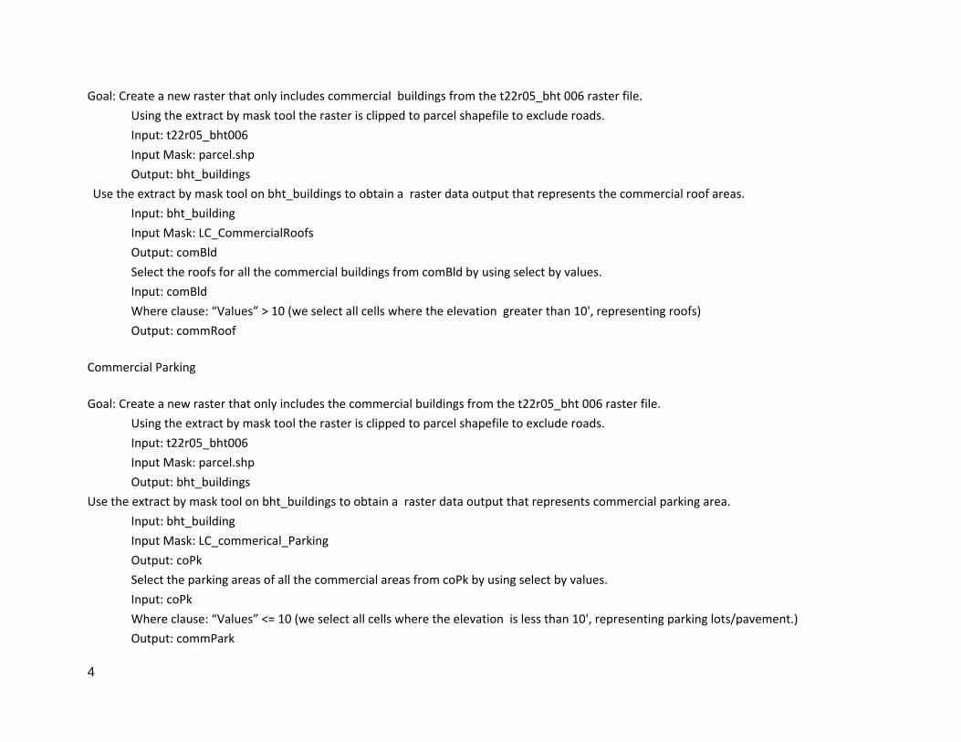
Goal: Create a new raster that only includes commercial buildings from the t22r05_bht 006 raster file.

Using the extract by mask tool the raster is clipped to parcel shapefile to exclude roads.




Use the extract by mask tool on bht_buildings to obtain a raster data output that represents the commercial roof areas.

Input: bht_building

Input Mask: LC_CommercialRoofs

Output: comBld

Select the roofs for all the commercial buildings from comBld by using select by values.

Input: comBld

Where clause: “Values” > 10 (we select all cells where the elevation greater than 10', representing roofs)

Output: commRoof

Commercial Parking

Goal: Create a new raster that only includes the commercial buildings from the t22r05_bht 006 raster file.





Use the extract by mask tool on bht_buildings to obtain a raster data output that represents commercial parking area.

Input: bht_building

Input Mask: LC_commerical_Parking

Output: coPk

Select the parking areas of all the commercial areas from coPk by using select by values.

Input: coPk

Where clause: “Values” <= 10 (we select all cells where the elevation is less than 10', representing parking lots/pavement.)

Output: commPark

Appendix B 5

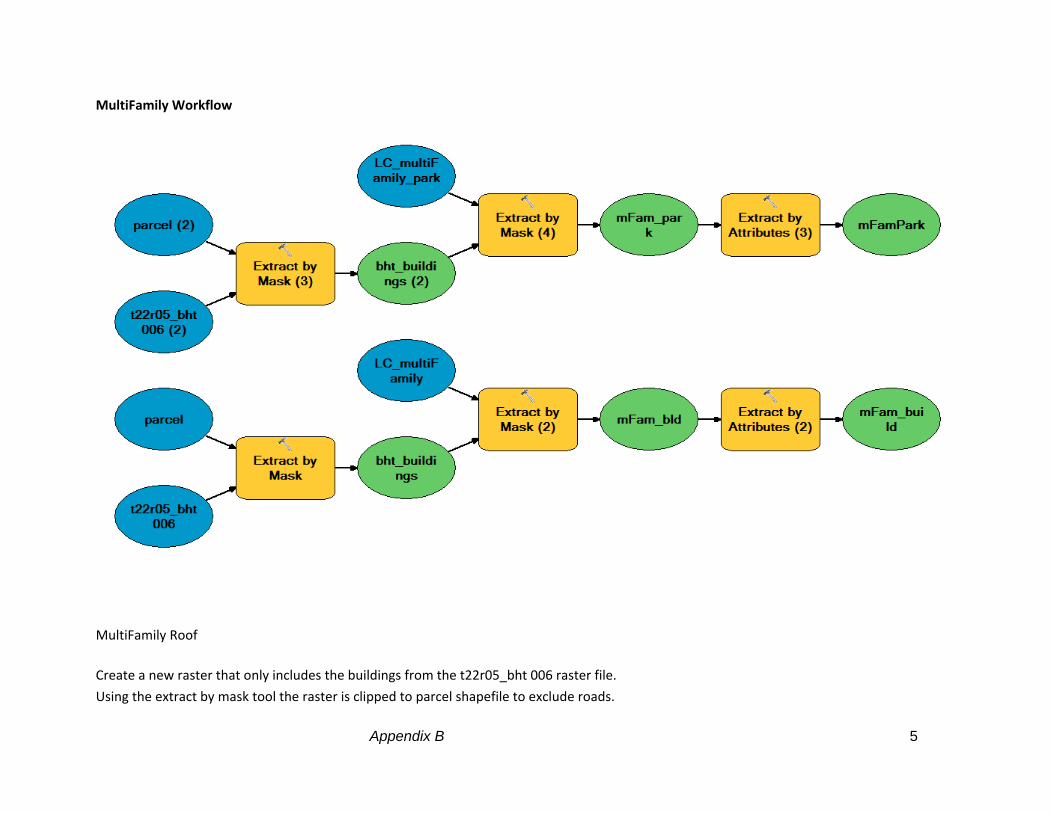
MultiFamily Workflow

MultiFamily Roof

Create a new raster that only includes the buildings from the t22r05_bht 006 raster file.


6




Extract by mask on bht_buildings to obtain a raster data output that represents MultiFamily roofs areas.

Input: bht_building

Input Mask: LC_multiFamily

Output: mFam_bld

We are then going to try and select the roofs of all the MultiFamily buildings from comBld by using select by values.

Input: mFam_bld

Where clause: “Values” > 6 (we we select all cells where the elevation is greater than or equal to 6', representing roofs; the 6'

threshold captures low‐hanging eaves.)

Output: mFam_build

MultiFamily Parking

Create a new raster that only includes the buildings from the t22r05_bht 006 raster file.





Extract by mask on bht_buildings obtain a raster data output that represents multifamily parking area.

Input: bht_building

Input Mask: LC_multiFamily_park

Output: mFam_park

We then select the parking areas of all the multi family areas from mfPk by using select by values.

Input: mFam_park

Where clause: “Values” <= 6 (we select all cells where the elevation is less than or equal to 6’.)

Output: mFamPark

Appendix B 7

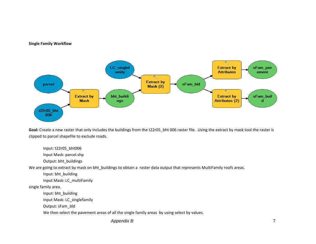
Single Family Workflow

Goal: Create a new raster that only includes the buildings from the t22r05_bht 006 raster file. Using the extract by mask tool the raster is

clipped to parcel shapefile to exclude roads.




We are going to extract by mask on bht_buildings to obtain a raster data output that represents MultiFamily roofs areas.

Input: bht_building

Input Mask: LC_multiFamily

single family area.

Input: bht_building

Input Mask: LC_singlefamily

Output: sFam_bld

We then select the pavement areas of all the single family areas by using select by values.

8

Input: sFam_bld

Where clause: “Values” <= 6 (we select anything where the elevation is less than or equal to 6’ to represent pavement.)

Output: sFam_pavment

We then select the building areas of all the single family areas by using select by values.

Input: sFam_bld

Where clause: “Values” > 6 (we we select all cells where the elevation is greater than or equal to 6', representing roofs; the 6' threshold

captures low‐hanging eaves.)

Output: sFam_build

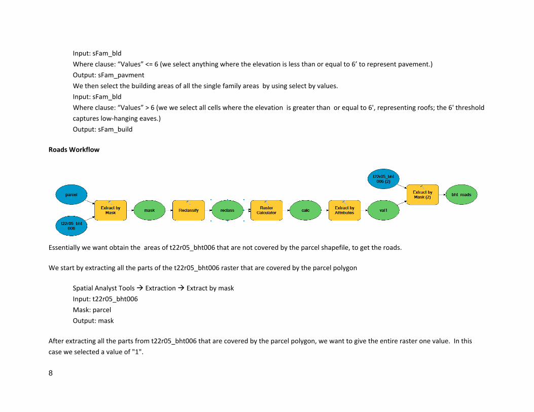
Roads Workflow

Essentially we want obtain the areas of t22r05_bht006 that are not covered by the parcel shapefile, to get the roads.

We start by extracting all the parts of the t22r05_bht006 raster that are covered by the parcel polygon

Spatial Analyst Tools Extraction Extract by mask


Mask: parcel

Output: mask

After extracting all the parts from t22r05_bht006 that are covered by the parcel polygon, we want to give the entire raster one value. In this

case we selected a value of "1".

Appendix B 9

Spatial Analyst Tools Reclass Reclassify

Input: Mask

Reclass Field: Value

Classify…

Method: Equal Interval

Classes: 1

Reclassification

New Values: 1

Output: Reclass

Once we set all the values to 1, we create another raster that will convert all the values of 1 to 0, and all the null values within the extent of

t22r05_bht006 will turn into 1. We change the values in reclass (raster created from the last step) from 1 to 0 because we are not interested in

the areas of the t22r05_bht006 that are covered by the parcel shapefile. We change all the null values in the extent of t22r05_bht006 because

that represents the areas we are interested in‐‐ in other words, those areas not covered by the parcel polygon).

Spatial Analyst Tools Map Algebra Raster Calculator

Expression: IsNull("reclass")

Output: Calc

We extract all the values of 1 to serve as a mask in the following step.

Spatial Analyst Tools Extraction Extract by Attributes

Input Raster: calc

Expression: "VALUE" = 1

Output: val1

Now we can extract the areas that are not covered by the parcel polygon by using val1 (raster created from the previous step) as the mask. The

output of this process will create a new raster of all the roads within the study area.

10

Spatial Analyst Tools Extraction Extract by Mask


Mask: val1

Output: bht_roads

Appendix C - 1 -

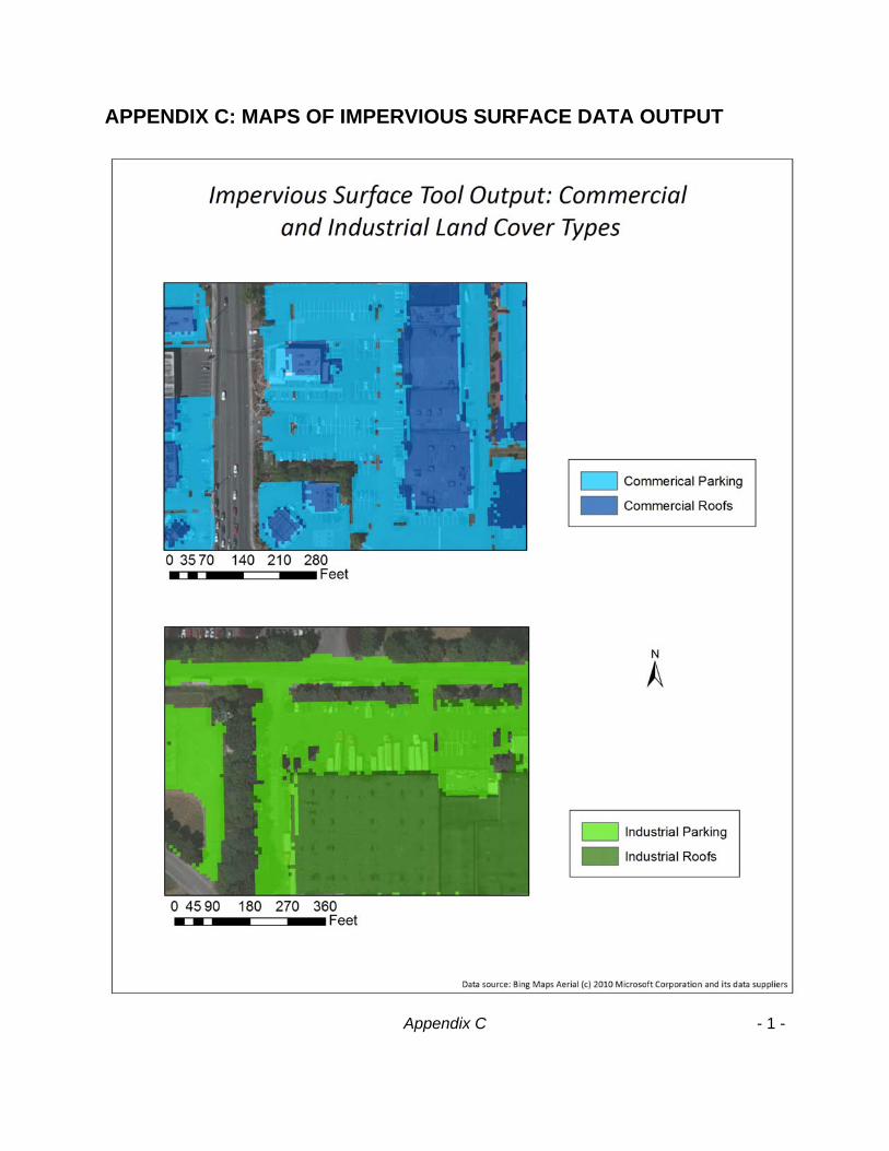
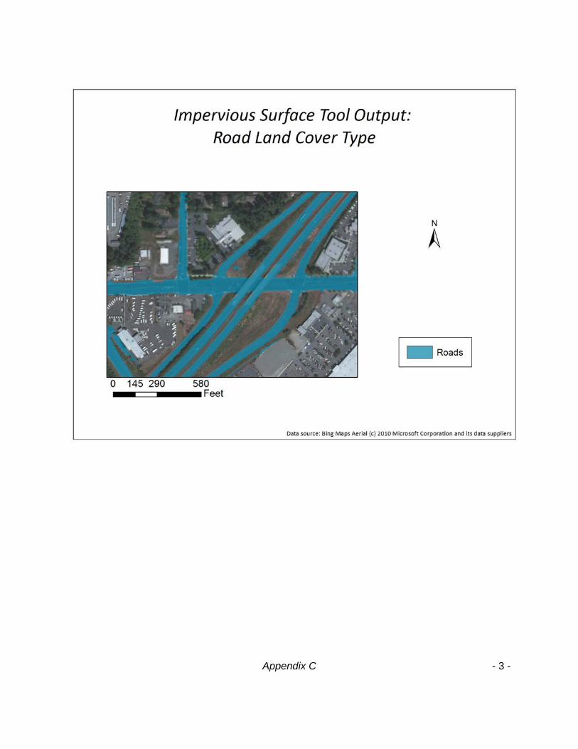
APPENDIX C: MAPS OF IMPERVIOUS SURFACE DATA OUTPUT

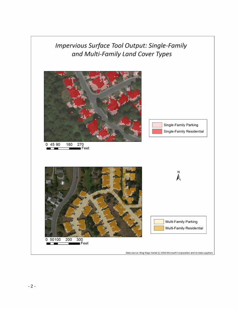
- 2 -

Appendix C - 3 -

Appendix D - 1 -

APPENDIX D: DETAILED FINANCIAL AND RISK ANALYSIS

FINANCIAL ANALYSIS

The financial analysis was conducted using the Financial Detail worksheets provided in Lerner et al’s

Building a Business Case for Geospatial Information Technology: A Practitioner’s Guide to Financial and

Strategic Analysis. These worksheets act as a template and include eleven variables of which many are

automated based on functions included in each cell. All of these variables were factored into each year

for the next 10 years of the project.

1. Inflation rate

2. Opportunity cost of capital

3. Job categories and descriptions

4. Average hourly rates for employees

5. Fringe rates

6. Avg. annual regular hours

7. Valuation method

8. FTEs dedicated to project in each project year

9. Contract and procurement costs

10. Productivity benefits per job category

11. Other benefits

The inflation rate used is 2.5% is the default provided in the worksheet and is comparable to Bureau of

Labor Statistics 2012 rates (http://www.bls.gov/data/). The second variable is opportunity costs of

capital at 5% which is a percentage that represents forgone investments by the project sponsor. The

analysis also includes job categories and descriptions. Three positions were identified in this analysis

which is a GIS programmer, hydrologist (environmental engineer) and supervisor. These categories are

used to provide details for labor costs for current and future employees that will spend efforts on

project development, but also any individuals that will benefit from the project. Job descriptions are

assessed to determine the hours or FTEs spent by employees for the tasks needed for project

implementation. In this case labor costs include annual salary which influences many other sub‐variables

among these is the valuation method which in this case per FTE. Fringe rates, or the burden rate, include

the cost of taxes, insurance and related overhead items for each employee. A rate of30% was used

which is based on estimates provided by the project sponsor. (Lerner et al, Appendix A, 2007). Contract

and procurement costs include items such as software and hardware upgrades or staff development and

training.

Ultimately the majority of the sponsor’s costs are determined by time needed for implementation which

includes a pilot project. The pilot project consists of the labor costs of the WLRD Science Section

integrating mapping tool output with their current water quality and storm‐water management models.

- 2 -

Benefits are the avoided labor or FTEs saved by implementing the mapping tool. Other benefits could

include new services that can be offered using the output of this tool, but those were not included in the

analysis.

The worksheets include Common Financial metrics such as net present value (NPV), the sum of present

values of all future cash flows, annualized return on investment (ROI), breakeven point and payback

period (Lerner et al, 2007). NPV is used at the key metric in this analysis because it is more

straightforward compared to other metrics. ROI can be somewhat deceptive and cannot be used in

comparing mutually exclusive investments. Another concern with ROI is that when subjective

assumptions are made in a financial analysis such as consolidating workload it can result in an inaccurate

ROI. Internal Rate of Return (IRR) is another important metric, but a high NPV does not always

correspond with a low IRR which becomes an issue when comparing two alternative projects or

conducting a sensitivity analysis as was done here. A sensitivity analysis was conducted by calculating

costs for a pilot project that focuses on WRIA 9 and then changing the hours to reflect the costs if the

pilot project focused on all of King County. The majority of the financial and strategic analysis will focus

on the resources need to complete the project for WRIA 9.

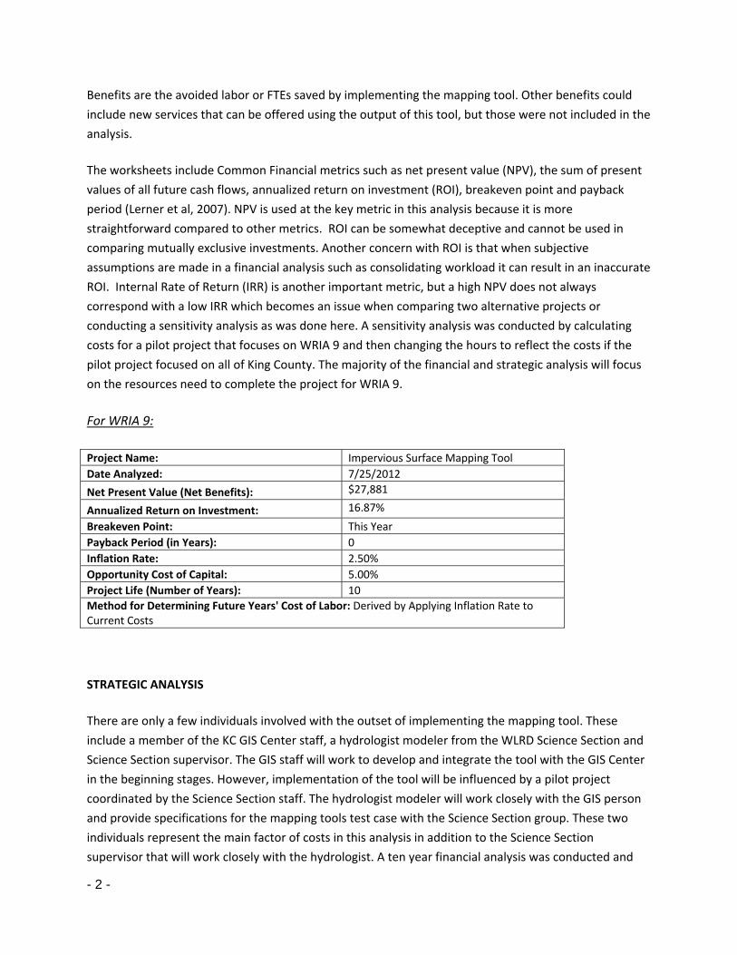
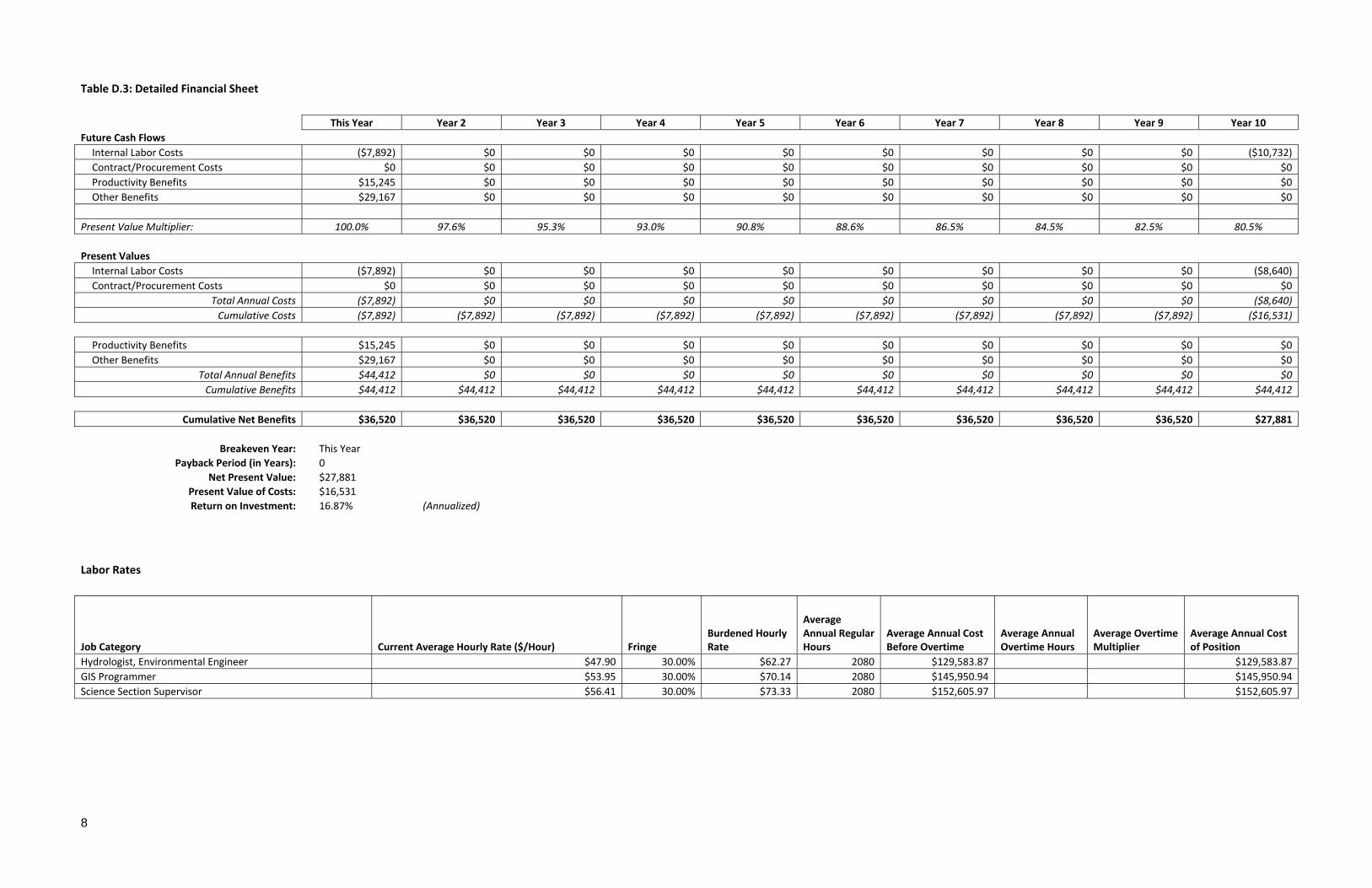
For WRIA 9:

Project Name: Impervious Surface Mapping Tool

Date Analyzed: 7/25/2012

Net Present Value (Net Benefits): $27,881

Annualized Return on Investment: 16.87%

Breakeven Point: This Year

Payback Period (in Years): 0

Inflation Rate: 2.50%

Opportunity Cost of Capital: 5.00%

Project Life (Number of Years): 10

Method for Determining Future Years' Cost of Labor: Derived by Applying Inflation Rate to Current Costs

STRATEGIC ANALYSIS

There are only a few individuals involved with the outset of implementing the mapping tool. These

include a member of the KC GIS Center staff, a hydrologist modeler from the WLRD Science Section and

Science Section supervisor. The GIS staff will work to develop and integrate the tool with the GIS Center

in the beginning stages. However, implementation of the tool will be influenced by a pilot project

coordinated by the Science Section staff. The hydrologist modeler will work closely with the GIS person

and provide specifications for the mapping tools test case with the Science Section group. These two

individuals represent the main factor of costs in this analysis in addition to the Science Section

supervisor that will work closely with the hydrologist. A ten year financial analysis was conducted and

Appendix D - 3 -

includes cost and benefit estimates for first year and subsequent years 5 and 10. These periods were

chosen because the Science Section will revisit with the GIS Center when new mapping tool input data

such as LiDAR data becomes available. This data can then be used to process new impervious surface

data. So the costs identified in the first year are then repeated every five year period as this new data

becomes available. While the tool will be fully implemented in the County’s GIS before these later years

there will be additional labor costs required for tool updates. These updates are associated with tool

modification necessary for its functionality with new hardware and software, such as newer versions of

ArcGIS.

The costs included in this analysis represent tool implementation costs such as upfront labor costs and

tool updates and maintenance, but does not consider other costs needed for developing specialized

impervious surface layers for other groups or departments within KC. One of the intangible benefits

gained by KC is the GIS Center’s ability to offer a new service to these other groups. (insert text on the

other applications described by Jim in last meeting? Or is that somewhere else?)

An increase in interrelated projects then becomes an intangible benefit of this mapping tool. WRLD

performance measures are influenced by many separate groups, but many of these groups will be able

to work together on the water management projects that require information on impervious surfaces of

King County. Finally, KC may also want to consider how the new impervious surface information created

by this tool can benefit outside agencies and organizations in the Puget Sound region.

Project Risks

Seven factors were adopted to highlight potential risks involved in implementing the tool. These include

technology, organizational interactions, constraints, stakeholders, overall complexity, project planning

project management and project resources. Described below is how each of these could negatively

impact the project’s success as well as ways of mitigating these effects. (Tomlinson, 2011)

Technology

There will be no additional hardware or software needed to implement the mapping tool and software

bugs or flaws should not be an issue for the first year. This may depend on the data used to operate the

tool because if the data is not in the correct format the tool will not function. This is unknown in later

applications of this tool as King County purchases new hardware and Esri releases new version of ArcGIS.

- 4 -

Current KC technology should be adequate but there is a risk that computer processing may be slow,

however it is not expected that the project sponsor will have to contract out because of this. This can be

mitigated by purchasing a small hardware upgrade such as increasing RAM.

Organizational Interactions

It is expected that there will be increased interaction between the KC GIS center and the WLRD: Science

Section, but sharing information is not an issue between departments. Because the information

produced by this tool has multiple applications KC GIS Center workload will increase for a short period of

time while they setup the tool and coordinate with different groups in the DNRP. Once the tool is

programmed is will only require a small number of minor changes to meet the needs of these other

groups.

Constraints

Surface water management fees generate $1 ‐ $2 million annually, which KC DNRP LWR uses to fund

both modeling and implementation of stormwater management activities. It is not expected that there

will be any risks regarding budget. The time needed for initial discussion regarding to the tool, tool

development and generating the desired data will not be substantial. Time spent by the GIS Programmer

position the first year could be as much as 150 hours or about three and half weeks. 140 hours is needed

by the Science Section Hydrologist and 10 hours by the Science Section Supervisor. It is important to

note that out of the 140 hours spent by the Hydrologist 120 hours is spent on integrating impervious

surface layers with SUSTAIN and HSPF models which is something not directly related to the

development of the tool. However, if testing is necessary this task could be included as a pilot project

for the tool.

Stakeholders

Stakeholder’s outside of the DNRP are not considered an immediate risk to the implementation of the

tool in this report. Interactions with organization, other government entities or the public will not take

place during tool development, however these groups may see value in the tool or the data layers

produced from the tool and ask the DNRP for information. Stakeholder involvement is somewhat

unforeseen at the moment and will depend on how the tool is applied and what sections of King County

will utilize it.

Overall complexity

As it exists now developing this tool and generating output is not complex in terms of time and funding

resources needed. Stakeholder involvement will be limited, there should be no violation of state or

federal regulations and vendors will not be used at least for the first year. However, it is expected that

this tool will be used every few years when new input data is acquired. Depending on how King County

Appendix D - 5 -

obtains input data they may be required to contract with outside organization. Time associated with this

activity is factored into updating/maintenance work included in the time table for years 5 and 10.

Project Planning

The planning is sufficient for implementing this tool into KC’s GIS environment. But the tool is developed

for ArcGIS version 10.1 so it will not function in earlier versions such as ArcGIS 9.3. Employees within the

Science Section group are currently using version 9.3, but they will not have an issue with viewing

impervious surface data layers in this layer

Project Management The project management methods are adopted from Professor Robert Aguirre of

the University of Washington, Roger Tomlinson’s book Thinking About GIS: Geographic information

System Planning for Managers and Paul Harmon’s book Business Process Change: A Guide for Business

Managers and BPM and Six Sigma Professionals which are both proven resources. Development of the

tool and future implementation is majorly contributed to the author’s knowledge and experiences as

well as to the methods and functions in Esri’s ArcGIS software which have been tested and used for

several years. Use of ArcGIS software provides built‐in accountability and quality control.

Project Resources

Trained staff at King County is not an issue as the tasks to be completed during project implementation

are within the abilities of the County. The employees of KC GIS Center have experience with Esri ArcGIS

and have the skills necessary to implement tool development and maintenance.

Other risks can include changes in the organization, such as departmental functions, but this should not

be a major concern. Responsibilities may increase for the DNRP such as assessing SWM fees per parcel.

Another risk could be project scheduling problems such as reasonable deadlines or developing reachable

milestones.

Overall the risks will not be too burdensome for the first year if King County implements the mapping

tool as outlined. Each of the risk identified above should be considered, but they are present in any

project and seem insignificant if compared to the benefits. There may be issues with updating the

mapping tool to generate new impervious surface data every few years. During times of use the tool will

need to be altered to function with new hardware and software that is adopted over those few years.

Values in the Labor Costs table below (Table D.1) were derived from the annual gross pay of KC

employees for each job category. The average gross pay of GIS programmer was determined by

averaging the salaries of the three employees in this position at KC.

- 6 -

(http://www.thenewstribune.com/soundinfo/kingsalaries/?appS

eession=343203812510513&cbSearchAgain=true) The fringe rate was determined by dividing the sum

of 2011 annual gross pay salary wage, taxes, insurance, and related overhead items for Curtis DeGasperi

, Hydrologist/Environmental Engineer for Surface Water Management Group, by their 2011 annual gross

pay salary wage.

($120,000 / $91,974) – 1 = 30% fringe rate

This was applied to all positions in the Labor Costs worksheet. The assumption is that positions are full‐

time equivalent (FTE) The benefit of labor costs saved was calculated with the assumption that it would

take a hydrologist at KC 100 hours per 200 acres for modeling a fully developed landscape using

SUSTAIN and 50 hours per 200 acres in a suburban landscape. Employee labor savings were estimated at

0.1 FTE per year or 10% of the hydrologist's workload.

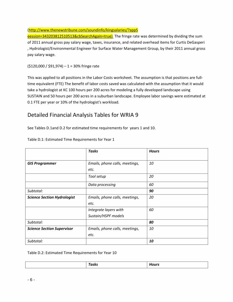
Detailed Financial Analysis Tables for WRIA 9

See Tables D.1and D.2 for estimated time requirements for years 1 and 10.

Table D.1: Estimated Time Requirements for Year 1

Tasks Hours

GIS Programmer Emails, phone calls, meetings,

etc.

10

Tool setup 20

Data processing 60

Subtotal: 90

Science Section Hydrologist Emails, phone calls, meetings,

etc.

20

Integrate layers with

Sustain/HSPF models

60

Subtotal: 80

Science Section Supervisor Emails, phone calls, meetings,

etc.

10

Subtotal: 10

Table D.2: Estimated Time Requirements for Year 10

Tasks Hours

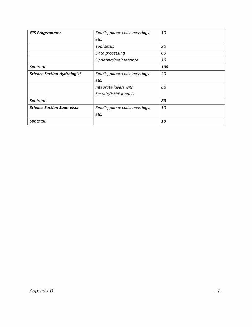
Appendix D - 7 -

GIS Programmer Emails, phone calls, meetings,

etc.

10

Tool setup 20

Data processing 60

Updating/maintenance 10

Subtotal: 100

Science Section Hydrologist Emails, phone calls, meetings,

etc.

20

Integrate layers with

Sustain/HSPF models

60

Subtotal: 80

Science Section Supervisor Emails, phone calls, meetings,

etc.

10

Subtotal: 10

8

Table D.3: Detailed Financial Sheet

This Year Year 2 Year 3 Year 4 Year 5 Year 6 Year 7 Year 8 Year 9 Year 10

Future Cash Flows

Internal Labor Costs ($7,892) $0 $0 $0 $0 $0 $0 $0 $0 ($10,732)

Contract/Procurement Costs $0 $0 $0 $0 $0 $0 $0 $0 $0 $0

Productivity Benefits $15,245 $0 $0 $0 $0 $0 $0 $0 $0 $0

Other Benefits $29,167 $0 $0 $0 $0 $0 $0 $0 $0 $0

Present Value Multiplier: 100.0% 97.6% 95.3% 93.0% 90.8% 88.6% 86.5% 84.5% 82.5% 80.5%

Present Values

Internal Labor Costs ($7,892) $0 $0 $0 $0 $0 $0 $0 $0 ($8,640)

Contract/Procurement Costs $0 $0 $0 $0 $0 $0 $0 $0 $0 $0

Total Annual Costs ($7,892) $0 $0 $0 $0 $0 $0 $0 $0 ($8,640)

Cumulative Costs ($7,892) ($7,892) ($7,892) ($7,892) ($7,892) ($7,892) ($7,892) ($7,892) ($7,892) ($16,531)

Productivity Benefits $15,245 $0 $0 $0 $0 $0 $0 $0 $0 $0

Other Benefits $29,167 $0 $0 $0 $0 $0 $0 $0 $0 $0

Total Annual Benefits $44,412 $0 $0 $0 $0 $0 $0 $0 $0 $0

Cumulative Benefits $44,412 $44,412 $44,412 $44,412 $44,412 $44,412 $44,412 $44,412 $44,412 $44,412

Cumulative Net Benefits $36,520 $36,520 $36,520 $36,520 $36,520 $36,520 $36,520 $36,520 $36,520 $27,881

Breakeven Year: This Year

Payback Period (in Years): 0

Net Present Value: $27,881

Present Value of Costs: $16,531

Return on Investment: 16.87% (Annualized)

Labor Rates

Job Category Current Average Hourly Rate ($/Hour) Fringe Burdened Hourly Rate

Average Annual Regular Hours

Average Annual Cost Before Overtime

Average Annual Overtime Hours

Average Overtime Multiplier

Average Annual Cost of Position

Hydrologist, Environmental Engineer $47.90 30.00% $62.27 2080 $129,583.87 $129,583.87

GIS Programmer $53.95 30.00% $70.14 2080 $145,950.94 $145,950.94

Science Section Supervisor $56.41 30.00% $73.33 2080 $152,605.97 $152,605.97

Appendix D 9

Labor Cost Multipliers1

Current Current Valuation Method

Year 1 Year 2 Year 3 Year 4 Year 5 Year 6 Year 7 Year 8 Year 9 Year 10

Job Category Average Hourly Rate

Average Annual Cost/FTE

Labor Cost Labor Cost Labor Cost Labor Cost Labor Cost Labor Cost Labor Cost Labor Cost Labor Cost Labor Cost

Hydrologist, Environmental Engineer

$62.27 $129,584 per FTE $129,583.87 $132,823.47 $136,144.05 $139,547.65 $143,036.35 $146,612.25 $150,277.56 $154,034.50 $157,885.36 $161,832.50

GIS Programmer

$70.14 $145,951 per FTE $145,950.94 $149,599.71 $153,339.70 $157,173.19 $161,102.52 $165,130.09 $169,258.34 $173,489.80 $177,827.04 $182,272.72

Science Section Supervisor

$73.33 $152,606 per FTE $152,605.97 $156,421.12 $160,331.65 $164,339.94 $168,448.44 $172,659.65 $176,976.14 $181,400.55 $185,935.56 $190,583.95

Valuation Method Options

Description

1Future Years' Labor cost derived by Applying Inflation Rate to Current Costs

Internal Labor Usage

Valuation Year 1 Year 2 Year 3 Year 4 Year 5 Year 6 Year 7 Year 8 Year 9 Year 10

Job Category Method Nature of Work Hrs or FTEs Hrs or FTEs Hrs or FTEs Hrs or FTEs Hrs or FTEs Hrs or FTEs Hrs or FTEs Hrs or FTEs Hrs or FTEs Hrs or FTEs

Hydrologist, Environmental Engineer per FTE

Provide GIS Programmer with parameters; overlay/integrate tool output with HSPF and SUSTAIN models; provided reports on information found 0.03846 0.00 0.00 0.00 0.00 0.00 0.00 0.00 0.00 0.03846

GIS Programmer per FTE

Coordinate with Hydrologist/other departments; run processes in ArcMap; provide impervious surface layers based on requests 0.01490 0.00 0.00 0.00 0.00 0.00 0.00 0.00 0.00 0.019712

Science Section Supervisor per FTE

Oversee Hydrologist/Science Section group; coordinate with Hydrologist on reports; review 0.00480 0.00 0.00 0.00 0.00 0.00 0.00 0.00 0.00 0.00480

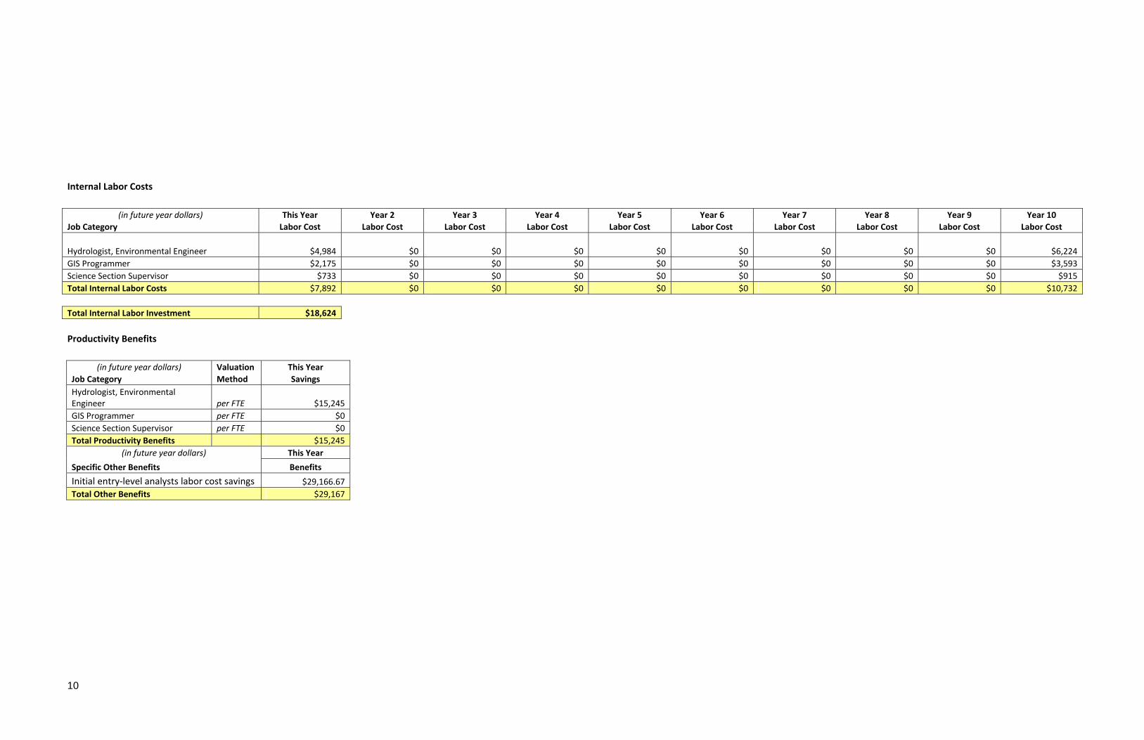
10

Internal Labor Costs

(in future year dollars) This Year Year 2 Year 3 Year 4 Year 5 Year 6 Year 7 Year 8 Year 9 Year 10

Job Category Labor Cost Labor Cost Labor Cost Labor Cost Labor Cost Labor Cost Labor Cost Labor Cost Labor Cost Labor Cost

Hydrologist, Environmental Engineer $4,984 $0 $0 $0 $0 $0 $0 $0 $0 $6,224

GIS Programmer $2,175 $0 $0 $0 $0 $0 $0 $0 $0 $3,593

Science Section Supervisor $733 $0 $0 $0 $0 $0 $0 $0 $0 $915

Total Internal Labor Costs $7,892 $0 $0 $0 $0 $0 $0 $0 $0 $10,732

Total Internal Labor Investment $18,624

Productivity Benefits

(in future year dollars) Valuation This Year

Job Category Method Savings

Hydrologist, Environmental Engineer per FTE $15,245

GIS Programmer per FTE $0

Science Section Supervisor per FTE $0

Total Productivity Benefits $15,245

(in future year dollars) This Year

Specific Other Benefits Benefits

Initial entry‐level analysts labor cost savings $29,166.67

Total Other Benefits $29,167

Documents

New Strategies for Impervious Surface Data Development