Embed Size (px)
Citation preview
Nicholas Shorter PID: N0425664 EEL 5825 – Pattern Recognition Project Assignment 1
Nicholas Shorter
PID: N0425664
EEL 5825 – Pattern Recognition
Project – Fuzzy Simplified Adaptive Resonance Theory
Friday December 9, 2005
Nicholas Shorter PID: N0425664 EEL 5825 – Pattern Recognition Project Assignment 2
Table of Contents 1. Detailed Paper Summary ................................................................................................................................... 4
1.1 Introduction.................................................................................................................................................. 4 1.2 Main Part...................................................................................................................................................... 4 1.3 Conclusions.................................................................................................................................................. 7 1.4 Own Impression of Paper Usefulness .......................................................................................................... 8 1.5 Shortened list of References ........................................................................................................................ 8 1.6 Comments Pertaining to list of References.................................................................................................. 8
2. Quantitative Measures of Performance for Clustering Algorithms .............................................................. 10 2.1 In Class Proposed Measures ...................................................................................................................... 10 2.2 Nicholas’ Proposed Measures.................................................................................................................... 11
3. Detailed Description of Fuzzy Simplified ART Network (SART) ................................................................. 12 3.1 Introduction................................................................................................................................................ 12 3.2 Previous Paper Reviews............................................................................................................................. 12 3.3 Main Paper (in which Fuzzy SART was proposed in) Review ................................................................. 13 3.4 Vector Degree of Match (activation) Function:......................................................................................... 13 3.5 User Defined Parameters ........................................................................................................................... 13 3.6 Additional Discussion................................................................................................................................ 14 3.7 Conclusions................................................................................................................................................ 15 3.8 Additional Materials .................................................................................................................................. 15
4. Algorithm Procedure........................................................................................................................................ 16 4.1 Fuzzy SART Training Phase ..................................................................................................................... 16 4.2 Fuzzy SART Performance Phase............................................................................................................... 17
5. Fuzzy SART Performance ............................................................................................................................ 19 5.1 A note on computation execution time ................................................................................................. 19 5.2 Computational Complexity of your Algorithm..................................................................................... 19 5.3 Observations about 2-D Data Sets ........................................................................................................ 19 5.4 User Defined Parameter Thresholds (Convergence Issues).................................................................. 20 5.5 New Abalone 500 Data Set................................................................................................................... 20 5.6 Nick Generated Data Set and execution times...................................................................................... 21 5.7 Pageblocks Data Set.............................................................................................................................. 22
Appendix............................................................................................................................................................... 24 1. Appendix 1 - Figures .................................................................................................................................... 25 2. Appendix 2 – Tables ..................................................................................................................................... 35 3. Appendix 3 – Equations................................................................................................................................ 40 4. Appendix 4 – Original Directions................................................................................................................. 43 5. Appendix 5 – Supplementary Discussion ..................................................................................................... 44
5.1 Use of Existing MATLAB Functions ........................................................................................................ 44 5.2 Performance: Note on flops command in MATLAB ............................................................................... 44 5.3 Computation Complexity Derivation......................................................................................................... 44
6. Appendix 6 – Data Set Testing Results ........................................................................................................ 47 6.1 g2c Data Set Results ............................................................................................................................. 48
6.1.1 g2c05 Data Set Results ................................................................................................................. 48 6.1.2 g2c15 Data Set Results ................................................................................................................. 52 6.1.3 g2c25 Data Set Results ................................................................................................................. 56 6.1.4 g2c40 Data Set Results ................................................................................................................. 60
6.2 g4c Data Set Results ............................................................................................................................. 64 6.2.1 g4c05 Data Set Results ................................................................................................................. 64 6.2.2 g4c15 Data Set Results ................................................................................................................. 68
Nicholas Shorter PID: N0425664 EEL 5825 – Pattern Recognition Project Assignment 3
6.2.3 g4c25 Data Set Results ................................................................................................................. 72 6.2.4 g4c40 Data Set Results ................................................................................................................. 76
6.3 irsdrg Data Set Results.......................................................................................................................... 80 6.4 New Abalon 500 Data Set Results........................................................................................................ 84 6.5 Nicholas Generated Data (1st generated set) .............................................................................................. 85 6.6 Nicholas Generated Data (2nd generated set) ............................................................................................. 89 6.7 pageblocks Data Set................................................................................................................................... 93 6.8 g6c Data Set Results ............................................................................................................................. 94
6.8.1 g6c05 Data Set Results ................................................................................................................. 94 6.8.2 g6c15 Data Set Results ................................................................................................................. 98 6.8.3 g6c25 Data Set Results ............................................................................................................... 102 6.8.4 g6c40 Data Set Results ............................................................................................................... 106
6.9 Generated Data Set 1 (no randomization)................................................................................................ 110 6.10 Generated Data Set 1 (with randomization)........................................................................................... 111
7 Appendix 7 – Matlab Code ......................................................................................................................... 112 7.1 Note on proj_x template...................................................................................................................... 112 7.2 fsart.m – training phase MATLAB function....................................................................................... 112 7.3 pfsart.m – performance phase MATLAB function............................................................................. 112
8 Appendix 8 – Reference List for Survey of Clustering Algorithms ............................................................ 121 9 Appendix 9 – Reference List for Project 3 ................................................................................................. 122

Nicholas Shorter PID: N0425664 EEL 5825 – Pattern Recognition Project Assignment 4
1. Detailed Paper Summary Instructions: Provide a detailed summary of one of these papers. The summary should include an Intro, a Main Part, Conclusions, Own impression of Paper Usefulness, and a shortened list of references. Chosen Paper: R. Xu, D. Wunch, II, “Survey of Clustering Algorithms”, IEEE Transactions on Neural Networks, Vol. 16, No. 3, May 2005, pp. 645-678. Title: Survey of Clustering Algorithms Author: R. Xu; D. Wunch, II Location: IEEE Explore Search (UCF Library Access) Abstract: Abstract—Data analysis plays an indispensable role for understanding various phenomena. Cluster analysis, primitive exploration with little or no prior knowledge, consists of research developed across a wide variety of communities. The diversity, on one hand, equips us with many tools. On the other hand, the profusion of options causes confusion. We survey clustering algorithms for data sets appearing in statistics, computer science, and machine learning, and illustrate their applications in some benchmark data sets, the traveling salesman problem, and bioinformatics, a new field attracting intensive efforts. Several tightly related topics, proximity measure, and cluster validation, are also discussed. Index Terms—Adaptive resonance theory (ART), clustering, clustering algorithm, cluster validation, neural networks, proximity, self-organizing feature map (SOFM). 1.1 Introduction R. Xu and D. Wunch’s Survey of Clustering Algorithms paper is a comprehensive review of a majority of clustering algorithms in existence up to date. The format of the paper is to develop some means of classifying groups of clustering algorithms and then going over the strengths and weaknesses of those groups. Following these strengths and weaknesses of the groups of clustering algorithms, some proposed improvements to those algorithms are then presented. One recursive theme, existent throughout the paper, is that no algorithm will produce optimum results for every application. 1.2 Main Part One important point referenced by Rui Xu and Donald Wunsch in the introduction of their “Survey of Clustering Algorithm” paper is there is no universal agreement up on the definition of clustering algorithms. Several somewhat vague definitions are attempted, but ultimately the nature of the algorithm, and therefore its definition classifying it, seems to vary from particular application to application. Furthermore, with a given problem there’s a given number of clustering algorithms particularly suited for that problem and with those clustering algorithms there’s an optimal range of adjustable parameters that can be tailored for that given problem. Ultimately, there is no universal clustering algorithm that will be optimal for all problem sets. Although no universal approach towards clustering exists, most algorithms in existence typically follow the following topology. A basic clustering process descriptive of all clustering algorithms is presented as a procedure containing four steps: (1) feature selection or extraction; (2) clustering algorithm design or selection; (3) cluster validation; (4) results interpretation. One distinctive classifier of clustering algorithms is whether or not that algorithm is dealing with supervised or unsupervised classification. In supervised classification, a set of input data, with a given dimensionality, is mapped to a discrete set of class labels via a mathematical function dependent on the input data and a set of adjustable parameters. The values of these parameters are in turn adjusted to minimize a given risk function for
Nicholas Shorter PID: N0425664 EEL 5825 – Pattern Recognition Project Assignment 5
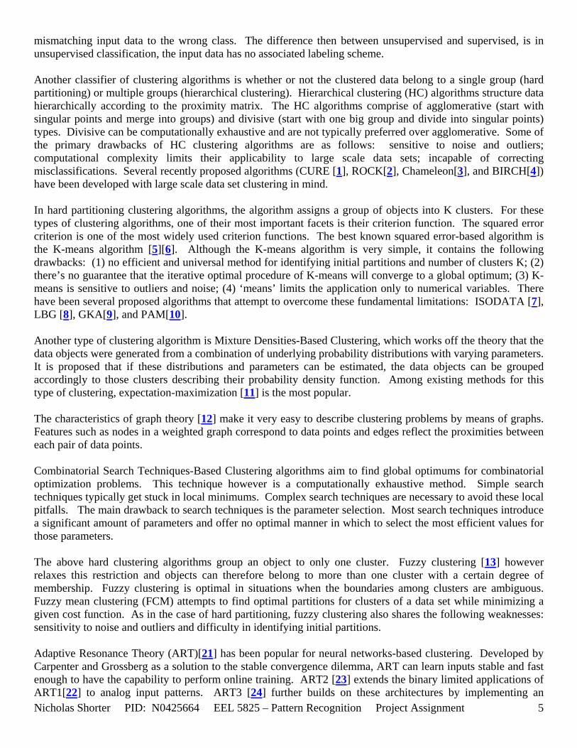
mismatching input data to the wrong class. The difference then between unsupervised and supervised, is in unsupervised classification, the input data has no associated labeling scheme. Another classifier of clustering algorithms is whether or not the clustered data belong to a single group (hard partitioning) or multiple groups (hierarchical clustering). Hierarchical clustering (HC) algorithms structure data hierarchically according to the proximity matrix. The HC algorithms comprise of agglomerative (start with singular points and merge into groups) and divisive (start with one big group and divide into singular points) types. Divisive can be computationally exhaustive and are not typically preferred over agglomerative. Some of the primary drawbacks of HC clustering algorithms are as follows: sensitive to noise and outliers; computational complexity limits their applicability to large scale data sets; incapable of correcting misclassifications. Several recently proposed algorithms (CURE [1], ROCK[2], Chameleon[3], and BIRCH[4]) have been developed with large scale data set clustering in mind. In hard partitioning clustering algorithms, the algorithm assigns a group of objects into K clusters. For these types of clustering algorithms, one of their most important facets is their criterion function. The squared error criterion is one of the most widely used criterion functions. The best known squared error-based algorithm is the K-means algorithm [5][6]. Although the K-means algorithm is very simple, it contains the following drawbacks: (1) no efficient and universal method for identifying initial partitions and number of clusters K; (2) there’s no guarantee that the iterative optimal procedure of K-means will converge to a global optimum; (3) K-means is sensitive to outliers and noise; (4) ‘means’ limits the application only to numerical variables. There have been several proposed algorithms that attempt to overcome these fundamental limitations: ISODATA [7], LBG [8], GKA[9], and PAM[10]. Another type of clustering algorithm is Mixture Densities-Based Clustering, which works off the theory that the data objects were generated from a combination of underlying probability distributions with varying parameters. It is proposed that if these distributions and parameters can be estimated, the data objects can be grouped accordingly to those clusters describing their probability density function. Among existing methods for this type of clustering, expectation-maximization [11] is the most popular. The characteristics of graph theory [12] make it very easy to describe clustering problems by means of graphs. Features such as nodes in a weighted graph correspond to data points and edges reflect the proximities between each pair of data points. Combinatorial Search Techniques-Based Clustering algorithms aim to find global optimums for combinatorial optimization problems. This technique however is a computationally exhaustive method. Simple search techniques typically get stuck in local minimums. Complex search techniques are necessary to avoid these local pitfalls. The main drawback to search techniques is the parameter selection. Most search techniques introduce a significant amount of parameters and offer no optimal manner in which to select the most efficient values for those parameters. The above hard clustering algorithms group an object to only one cluster. Fuzzy clustering [13] however relaxes this restriction and objects can therefore belong to more than one cluster with a certain degree of membership. Fuzzy clustering is optimal in situations when the boundaries among clusters are ambiguous. Fuzzy mean clustering (FCM) attempts to find optimal partitions for clusters of a data set while minimizing a given cost function. As in the case of hard partitioning, fuzzy clustering also shares the following weaknesses: sensitivity to noise and outliers and difficulty in identifying initial partitions. Adaptive Resonance Theory (ART)[21] has been popular for neural networks-based clustering. Developed by Carpenter and Grossberg as a solution to the stable convergence dilemma, ART can learn inputs stable and fast enough to have the capability to perform online training. ART2 [23] extends the binary limited applications of ART1[22] to analog input patterns. ART3 [24] further builds on these architectures by implementing an

Nicholas Shorter PID: N0425664 EEL 5825 – Pattern Recognition Project Assignment 6
optimized search strategy for hierarchical structures. The ARTMAP [20] system, equipped with an ARTa and ARTb-ART modules realizes a system utilized for supervised classifications. Via the tweaking of the vigilance parameter, the match tracking algorithm guarantees consistency for category prediction for both models. Larger values of the vigilance parameter yield more clusters. As the value of the vigilance parameter approaches zero, the algorithm becomes a nearest neighbor approach. Fuzzy ART (FA)[33], which is ART incorporating fuzzy set theory, has the ability for online training, stable fast learning, and atypical pattern detection. Unfortunately FA suffers from minimal robustness to noise and has the weakness of representing clusters as hyper-rectangles. Several algorithms have been proposed to circumvent these inherent weaknesses: Gaussian ART (GA)[14]; Hypersphere ART (HA)[15]; SART[37]; Fuzzy SART[31]; and FOSART. Kernel based learning algorithms center on Cover’s theorem: nonlinear, complex separable patterns become linear when transformed into a higher dimensional feature space. The use of Mercer’s theorem by calculating the inner-product kernel aids us in avoiding the exhaustive process to explicitly detail the nonlinear mapping. [Table 1] enumerates the advantages and disadvantages of kernel based clustering. Sequential data are ordered data with some of the following characteristics: variable length; dynamic behaviors; time constraints; large volumes; etc. Three general categories encompass the majority of existent sequential clustering algorithms: (1) Sequence Similarity; (2) Indirect Sequence Clustering; (3) Statistical Sequence Clustering. Sequence similarity methods use measures of distance (or similarity) between pairs of sequences followed by proximity based clustering algorithms used to group those sequences. Indirect sequence clustering methods extract groups of features from the sequences and map them onto a transformed feature space, where classical vector space-based clustering algorithms can operate on them to form clusters. It should be noted sequential clustering algorithms (1) and (2) are typically applied to sequential data composed of alphabets. Statistical sequence clustering methods however are optimal for applications dealing with numerical or categorical sequences. As the size, dimensionality and inherently the complexity of the data set examined increases, the scalability of the algorithm becomes more important. Classical hierarchical clustering algorithms are not optimal for large scale data sets due to their computational complexity. However, because K-means are efficient for clustering large scale data sets, much effort is currently spent in improving on the draw backs of the method. Several algorithms have been proposed that are capable of scaling their computational complexity linearly with the input size of the data set. Methods for such linearly scaling approaches are as follows: random sampling approach; randomized search approach; condensation-based approach; density based spatial clustering; and grid based approach. Most of these algorithms however suffer from inefficiency when dealing with data sets with high dimensionality. If efficiently possible, one way of decreasing the complexity of the data set is via a reduction in its dimensionality. Reducing the dimensions of the input data set decreases both the computational cost of the algorithm operating on that data set and enables the user with the ability to visually comprehend the data set. However, compression usually comes with a loss of information which may distort the real clusters. Numerous clustering algorithms request K, from the user, as an input. Selecting too many clusters will add unnecessary complexity making the result difficult to interpret and analyze. If not enough clusters are selected, the lack of information will distort the final product. The following procedures aid in estimating an optimal K value: (1) visualization of the data set; (2) construction of certain indices; (3) optimization of criterion function under probabilistic mixture model framework; (4) other heuristic approaches. The first procedure, visualization of the data set, entails visual inspection of a given data set on Euclidean space. This procedure however is limited to data sets that can be projected on to 2 or 3 dimensional space. The second procedure stresses the compactness of intra-cluster and isolation of inter-cluster and makes use of a variety of different factors: defined square error; geometric statistical properties of the data; the number of patterns; the dis-similarity (or similarity) and the number of clusters. Miligan and Cooper compared and ranked 30 indices according to their
Nicholas Shorter PID: N0425664 EEL 5825 – Pattern Recognition Project Assignment 7
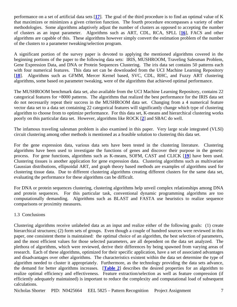
performance on a set of artificial data sets [17]. The goal of the third procedure is to find an optimal value of K that maximizes or minimizes a given criterion function. The fourth procedure encompasses a variety of other methodologies. Some algorithms adaptively adjust the number of clusters as opposed to accepting the number of clusters as an input parameter. Algorithms such as ART, CDL, RCA, SPLL [16], FACS and other algorithms are capable of this. These algorithms however simply convert the estimation problem of the number of the clusters to a parameter tweaking/selection program. A significant portion of the survey paper is devoted to applying the mentioned algorithms covered in the beginning portions of the paper to the following data sets: IRIS, MUSHROOM, Traveling Salesman Problem, Gene Expression Data, and DNA or Protein Sequences Clustering. The iris data set contains 50 patterns each with four numerical features. This data set can be downloaded from the UCI Machine Learning Repository [18]. Algorithms such as GFMM, Mercer Kernel based, SVC, CDL, RHC, and Fuzzy ART clustering algorithms, some based on parameter tweaking, were of the algorithms that achieved optimal performance. The MUSHROOM benchmark data set, also available from the UCI Machine Learning Repository, contains 22 categorical features for +8000 patterns. The algorithms that realized the best performance for the IRIS data set do not necessarily repeat their success in the MUSHROOM data set. Changing from a 4 numerical feature vector data set to a data set containing 22 categorical features will significantly change which type of clustering algorithm to choose from to optimize performance. For this data set, K-means and hierarchical clustering works poorly on this particular data set. However, algorithms like ROCK [2] and SBAC do well. The infamous traveling salesman problem is also examined in this paper. Very large scale integrated (VLSI) circuit clustering among other methods is mentioned as a feasible solution to clustering this data set. For the gene expression data, various data sets have been tested in the clustering literature. Clustering algorithms have been used to investigate the functions of genes and discover their purpose in the genetic process. For gene functions, algorithms such as K-means, SOFM, CAST and CLICK [19] have been used. Clustering tissues is another application for gene expression data. Clustering algorithms such as multivariate Gaussian distributions, ellipsoidal ART, and graph theory based methods are examples of algorithms used for clustering tissue data. Due to different clustering algorithms creating different clusters for the same data set, evaluating the performance for these algorithms can be difficult. For DNA or protein sequences clustering, clustering algorithms help unveil complex relationships among DNA and protein sequences. For this particular task, conventional dynamic programming algorithms are too computationally demanding. Algorithms such as BLAST and FASTA use heuristics to realize sequence comparisons or proximity measures. 1.3 Conclusions Clustering algorithms receive unlabeled data as an input and realize either of the following goals: (1) create hierarchical structures; (2) form sets of groups. Even though a couple of hundred sources were reviewed in this paper, one consistent theme is maintained: the optimal choice of an algorithm, the best selection of parameters, and the most efficient values for those selected parameters, are all dependent on the data set analyzed. The plethora of algorithms, which were reviewed, derive their differences by being spawned from varying areas of research. Each of these algorithms, optimized for their specific application, have a set of associated advantages and disadvantages over other algorithms. The characteristics existent within the data set determine the type of algorithm needed to cluster it appropriately. Furthermore, as the technology providing the data sets advance, the demand for better algorithms increases. [Table 2] describes the desired properties for an algorithm to realize optimal efficiency and effectiveness. Feature extraction/selection as well as feature compression (if efficiently adequately maintained) is important to reduce the complexity and computational load of subsequent calculations.

Nicholas Shorter PID: N0425664 EEL 5825 – Pattern Recognition Project Assignment 8
1.4 Own Impression of Paper Usefulness If one was assigned a data set with the goal of clustering that data set, one excellent resource to get started with would be this survey paper. The paper meticulously lists various types of data set characteristics and which algorithms would realize maximum performance on those data sets. Furthermore, the paper comprehensively summarizes everything in the clustering literature to date, highlighting the strengths and weaknesses of certain algorithms and proposes algorithms that improve on weaknesses of other algorithms. The survey paper’s enormous reference list provides a library of sources to consult to for items of interest outlined in the paper. As with many engineering applications, for clustering there is no universal algorithm that will deliver optimal performance for all clustering applications. Algorithms instead have optimal performance for a certain field of given applications with certain parameter ranges. From this paper, one can extract a list of properties of a given data set that will affect the selection of the optimal choice for a clustering algorithm to cluster that particular data set. A proposed list is provided as [Table 3]. The paper went on to extensively describe initial clustering, K, estimation techniques. Some algorithms, Fuzzy ARTMAP included, convert this problem of initial cluster estimation into a parameter tweaking problem. The survey paper provides good sources, [17] in particular, for tackling this issue of initial parameter estimation. As a preprocessing technique, another important issue mentioned was feature compression. If it is possible to efficiently compress features of a given data set with minimal information loss, feature compression/reduction can yield a decrease in computational demand and complexity in subsequent calculations. A general strategy one could devise for selecting an appropriate algorithm for clustering data could be summarized by the steps below, derived form the survey paper:
1. Consider the parameters listed in [Table 3] 2. Based on the data set, perform the necessary pre-processing techniques: complement encoding;
normalization of inputs; feature compression; feature reduction; feature encoding; etc. 3. Based on the algorithm, partition the data into a training set and test set 4. Use the test set to optimize any tweak-able parameters associated with the algorithm 5. Test the algorithm on the test set
Preprocessing techniques, clustering selection, and parameter optimization are all mentioned in the paper with sources provided. Having a survey paper to outline a strategy, in addition to providing a plethora of other sources related to various components of the outlined strategy is indeed a valuable paper. Xu and Wunsch’s Survey of Clustering Algorithms paper is a very useful source for selecting and implementing or even designing a clustering algorithm. 1.5 Shortened list of References Note: The recommended Reference List [8] for this survey paper review can be found in section 6 of the Appendix. Section [9] of the appendix refers to the content referenced for the rest of this project. 1.6 Comments Pertaining to list of References The following is a brief commentary on several of the noteworthy sources cited in the survey paper review reference list. Reference [18] contains a link to the UCI Machine Learning Repository where a couple of the

Nicholas Shorter PID: N0425664 EEL 5825 – Pattern Recognition Project Assignment 9
databases described in this paper are available for download. Miligan and Cooper compared and ranked 30 indices, for determining an optimal initial number of K clusters, according to their performance on a set of artificial data sets [17]. References [20],[21],[22],[23], and [24] all refer to Carpenter and Grossberg’s work on their original Adaptive Resonance Theory algorithm and their updated improvements/modifications. A great source for downloading a good majority of Carpenter’s work on ART can be found at [35]. A modification on those ART algorithms is presented in [15]. The CURE[1], ROCK[2], Chameleon[3], and BIRCH[4] algorithms are mentioned several times throughout the course of the paper. Citations for those algorithms have been provided accordingly.

2. Quantitative Measures of Performance for Clustering Algorithms In order to gauge the performance of the proposed clustering algorithm on the test data bases provided, the following quantitative measures of performance are suggested: 2.1 In Class Proposed Measures 1. Average Mean Squared Distance
J
1
Nc
j 1
Sj
x
x⎯
mj⎯
−( )2∑=
∑= [Equation 1]
Where: Nc: the number of clusters that were created x: A data point from your data set mj: The jth cluster center Sj: the set of data points that belong the jth cluster This measure defines the average mean squared distance from the created cluster centers to the data points belonging to the cluster. This metric describes how close the data belonging to a given cluster is positioned to the cluster’s center. 2. Intra Cluster Distance
D2 x1( ) x2( ),⎡⎣ ⎤⎦⎡⎣ ⎤⎦⎯
1k k 1−( )⋅
1
k
j 1
k
i 1
n
k
xkj xk
i−⎛
⎝⎞⎠
2
∑=
∑=
∑=
⋅
[Equation 2] The above metric measures the average sum of distances of objects in the same clusters. This is different from the above metric in that this measures the average distance between all data points with all other data points within the same cluster. An optimal clustering algorithm will seek to create clusters that will minimize the intra cluster distances while maximizing the inter clustering distance. 3. Inter Cluster Distance The inter cluster distance is the distance between the centers of clusters. The center of the cluster is defined as the centroid for spherical clusters. This metric is a measure of how close cluster centers are to one another. An ideal clustering algorithm will aim to create cluster centers such that this distance is maximized while minimizing intra cluster distance. 4. Split the data into training and testing sets Optimize the algorithm’s user defined parameters in the training set to yield the best classification rate. Then test the performance phase of the algorithm on unforeseen data – the testing set. Report the classification rate for the both the training and performance phases. This metric describes how accurately the clustering algorithm is able to cluster various types of classes within a given data set. For Fuzzy SART, first the algorithm is trained on a partition of the entire data set (this partition must have validation data). Then Fuzzy SART clusters unforeseen data that is of similar structure to the training data. 5. How many parameters do you need to tweak to make your algorithm work? The more necessary parameters needing adjustments, the more complicated the algorithm. Nicholas Shorter PID: N0425664 EEL 5825 – Pattern Recognition Project Assignment 10

Nicholas Shorter PID: N0425664 EEL 5825 – Pattern Recognition Project Assignment 11
This question will be addressed in both this section and the performance section with the same answer. The algorithm only has 2 user defined parameters, both of which have intuitive physical meaning (described in the following section). One of the key features of Fuzzy Simplified ART is its ease of use due to only having 2 user defined parameters. 6. Computational complexity of your clustering algorithm. Track the following number of operations: multiplications (divisions), additions (subtractions), comparison operators. The number of operations should be proportional to the number of clusters and data points. This metric reports the computational complexity of a given algorithm. For algorithms operating on large data sets, this measure can be important. 2.2 Nicholas’ Proposed Measures 7. Execution Time Computational demand of algorithm should be proportional to execution time of algorithm. The execution time for each data set will be reported in the performance section of the document. 8. Repeatability with Random Ordered Inputs Can the algorithm generate the same clusters for the same data set presented regardless of the order it is presented? The inputs to the Fuzzy SART algorithm will be randomized. Then each point will be checked to make sure the same class label is assigned to that point. 9. Number of Epochs for Convergence How many epochs does it take for algorithm to converge to a solution? Note, for Fuzzy SART this parameter is only applicable to the training phase (no epochs are implemented in the performance phase). The computational load of a Fuzzy ART algorithm is proportional to the number of necessary epochs the algorithm must cycle through to converge to a solution.
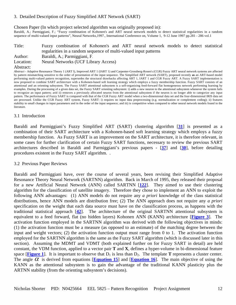
3. Detailed Description of Fuzzy Simplified ART Network (SART) Chosen Paper (In which project selected algorithm was originally proposed in): Baraldi, A.; Parmiggiani, F.; “Fuzzy combination of Kohonen's and ART neural network models to detect statistical regularities in a random sequence of multi-valued input patterns”, Neural Networks,1997., International Conference on, Volume 1, 9-12 June 1997 pp.281 - 286 vol.1 Title: Fuzzy combination of Kohonen's and ART neural network models to detect statistical
regularities in a random sequence of multi-valued input patterns Author: Baraldi, A.; Parmiggiani, F. Location: Neural Networks (UCF Library Access) Abstract: Abstract - Adaptive Resonance Theory 1 (ART l), Improved ART 1 (IART 1) and Carpenter-Grossberg-Rosen's (CGR) Fuzzy ART neural network systems are affected by pattern mismatching sensitive to the order of presentation of the input sequence. The Simplified ART network (SART), proposed recently as an ART-based model performing multi-valued pattern recognition, supersedes the structural drawbacks affecting ART 1, IART 1 and CGR Fuzzy ART. A Fuzzy SART implementation is now proposed to combine SART architecture with a Kohonen-based soft learning strategy which employs a fuzzy membership function. Fuzzy SART consists of an attentional and an orienting subsystem. The Fuzzy SART attentional subsystem is a self-organizing feed-forward flat homogeneous network performing learning by examples. During the processing of a given data set, the Fuzzy SART orienting subsystem: i) adds a new neuron to the attentional subsystem whenever the system fails to recognize an input pattern; arid ii) removes a previously allocated neuron from the attentional subsystem if the neuron is no longer able to categorize any input pattern. The performance of Fuzzy SART is compared with that of the CGR Fuzzy ART model when a two-dimensional data set and the four-dimensional IRIS data set are processed. Unlike the CGR Fuzzy ART system, Fuzzy SART: i) requires no input data preprocessing (e.g. normalization or complement coding); ii) features stability to small changes in input parameters and in the order of the input sequence; and iii) is competitive when compared to other neural network models found in the literature. 3.1 Introduction Baraldi and Parmiggiani’s Fuzzy Simplified ART (SART) clustering algorithm [31] is presented as a combination of their SART architecture with a Kohonen-based soft learning strategy which employs a fuzzy membership function. As Fuzzy SART is an improvement on the SART architecture, it is therefore relevant, in some cases for further clarification of certain Fuzzy SART functions, necessary to review the previous SART architectures described in Baraldi and Parmiggiani’s previous papers - [37] and [30], before detailing procedures existent in the Fuzzy SART algorithm. . 3.2 Previous Paper Reviews Baraldi and Parmiggiani have, over the course of several years, been revising their Simplified Adaptive Resonance Theory Neural Network (SARTNN) algorithm. Back in March of 1995, they released their proposal for a new Artificial Neural Network (ANN) called SARTNN [122]. They aimed to use their clustering algorithm for the classification of satellite imagery. Therefore they chose to implement an ANN to exploit the following ANN advantages: (1) ANN models do not require any a priori knowledge of the class statistical distributions, hence ANN models are distribution free; (2) The ANN approach does not require any a priori specification on the weight that each data source must have on the classification process, as happens with the traditional statistical approach [42]. The architecture of the original SARTNN attentional subsystem is equivalent to a feed forward, flat (no hidden layers) Kohonen ANN (KANN) architecture [Figure 3]. The activation function employed in the SARTNN algorithm was derived with the following objectives in minds: (1) the activation function must be a measure (as opposed to an estimate) of the matching degree between the input and weight vectors; (2) the activation function output must range from 0 to 1. The activation function employed for the SARTNN algorithm is the same as the Fuzzy SART algorithm (which is discussed later in this section). Assuming the MDMT and VDMT (both explained further on for Fuzzy SART in detail) are held constant, the VDM function, applied to a vector pair T and X, defines a hyper-volume in bi-dimensional feature space [Figure 1]. It is important to observe that D1 is less than D2. The template T represents a cluster center. The angle α is derived from equations [Equation 15] and [Equation 16]. The main objective of using the KANN as the attentional subsystem is to gain the advantage of the traditional KANN plasticity plus the ARTNN stability (from the orienting subsystem’s decisions).
Nicholas Shorter PID: N0425664 EEL 5825 – Pattern Recognition Project Assignment 12

Less than a year later, Baraldi and Parmiggiani published another paper [30], presenting an improvement on their original SARTNN algorithm with their new SARTNN2 model. The SARTNN2 model improves the Winner Takes All (WTA) strategy of the SARTNN1 attentional subsystem by employing Kohonen’s short cut algorithm to perform topologically ordered mapping [43]. An ANN, by definition, achieves topologically correct (ordered) mapping when Processing Elements (PEs), spatially situated close to one another, are activated by input patterns which are mutually spatially close to one another in the event measurement space. Kohonen, however, revealed that the same ordered mapping can be realized when following these procedures (bubble strategy): (1) centering neighboring PEs, belonging to the resonance domain, on the winning neuron (category) to obtain the same input pattern; (2) decreasing the resonance domain through the acquisition phase. The decrease in the size of the resonance domain criterion is employed by the following functions in the SARTNN2 model: [Equation 33] and [Equation 34]. Later, in Fuzzy SART, these functions evolve to [Equation 22] and [Equation 23], which are now dependent on the newly employed membership function [Equation 9]. 3.3 Main Paper (in which Fuzzy SART was proposed in) Review Baraldi and Parmiggiani present the Fuzzy Simplified ART (SART) clustering algorithm [31] as an improvement on the structural drawbacks of Fuzzy ART (FA)[33]. Fuzzy SART has several advantages over FA, listed as follows: (1) no data pre-processing required; (2) maintains stability for small changes in input parameters and changes in the order of the input sequence. The algorithm also has competitive clustering accuracies and performance when compared against other algorithms found in the literature. The Fuzzy SART model is a SART-based system employing a soft-max learning strategy [Equation 3 and Equation 4] with a neuron membership function [Equation 9]. The neuron membership function appears in the resonance domain definition equations ( [Equation 22], [Equation 23] )and the learning rate update equations, in both winner [Equation 4] and non winner neuronal learning rates [Equation 3]. The activation function, Vector Degree of Match (VDM) [Equation 21], calculates the similarity between the input vector X and the template vector T by detecting in parallel their degree of “chromatic” and “achromatic” similarity. The T vector’s scalar components correspond to the weights of the bottom-up connections that link the input units to the output neurons. The T vector represents the long term memory associated with that output neuron. The comparison between the two vectors, T and X, is done via the NVD metric [37], which yields a Vector Degree of Match value (VDM) [Equation 11] equal to the normalized measurement of similarity between the two vectors. 3.4 Vector Degree of Match (activation) Function: The Vector Degree of Match function consists of the product of two functions: (1) the Module Degree of Match (MDM) [Equation 13] and (2) Angle Degree of Match (ADM) [Equation 15]. Both of these functions have values that range from 0 to 1 corresponding to their input component similarity. In other words, MDM approaches unity as the two vectors inputted to the function approach equal moduli. Note, modulus of a vector is the equivalent of the magnitude of a vector [i.e. |(x,y)| = sqrt(x^2+y^2) ]. As the inputs (typically the template vector T and the input vector X) approach the same orientation and direction, the ADM approaches unity. The VDM is a nonlinear combination of both the MDM and ADM, such that the VDM is smaller than the smallest term between the MDM and ADM. The VDM is a dimensionless percent value capable of adjusting the width of its domain of acceptance to the pair of vectors being compared [30]. The VDM also satisfies the commutative property, i.e., VDM(T,X) = VDM(X,T). 3.5 User Defined Parameters The two user defined parameters are τ and VDMT (the Vector Degree of Match Threshold, also called the vigilance parameter). The vigilance parameter, VDMT, restricts the accepted range of similarity in which the Nicholas Shorter PID: N0425664 EEL 5825 – Pattern Recognition Project Assignment 13
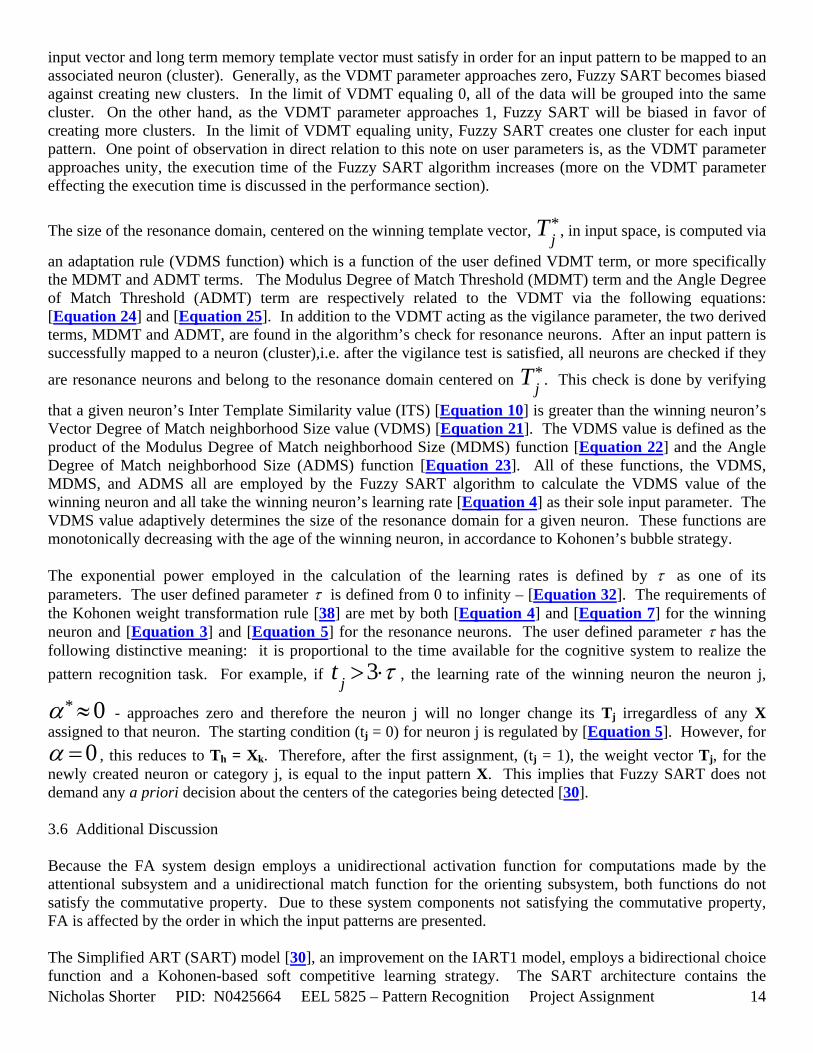
input vector and long term memory template vector must satisfy in order for an input pattern to be mapped to an associated neuron (cluster). Generally, as the VDMT parameter approaches zero, Fuzzy SART becomes biased against creating new clusters. In the limit of VDMT equaling 0, all of the data will be grouped into the same cluster. On the other hand, as the VDMT parameter approaches 1, Fuzzy SART will be biased in favor of creating more clusters. In the limit of VDMT equaling unity, Fuzzy SART creates one cluster for each input pattern. One point of observation in direct relation to this note on user parameters is, as the VDMT parameter approaches unity, the execution time of the Fuzzy SART algorithm increases (more on the VDMT parameter effecting the execution time is discussed in the performance section).
The size of the resonance domain, centered on the winning template vector, , in input space, is computed via
an adaptation rule (VDMS function) which is a function of the user defined VDMT term, or more specifically the MDMT and ADMT terms. The Modulus Degree of Match Threshold (MDMT) term and the Angle Degree of Match Threshold (ADMT) term are respectively related to the VDMT via the following equations: [Equation 24
*jT
] and [Equation 25]. In addition to the VDMT acting as the vigilance parameter, the two derived terms, MDMT and ADMT, are found in the algorithm’s check for resonance neurons. After an input pattern is successfully mapped to a neuron (cluster),i.e. after the vigilance test is satisfied, all neurons are checked if they
are resonance neurons and belong to the resonance domain centered on . This check is done by verifying
that a given neuron’s Inter Template Similarity value (ITS) [Equation 10
*jT
] is greater than the winning neuron’s Vector Degree of Match neighborhood Size value (VDMS) [Equation 21]. The VDMS value is defined as the product of the Modulus Degree of Match neighborhood Size (MDMS) function [Equation 22] and the Angle Degree of Match neighborhood Size (ADMS) function [Equation 23]. All of these functions, the VDMS, MDMS, and ADMS all are employed by the Fuzzy SART algorithm to calculate the VDMS value of the winning neuron and all take the winning neuron’s learning rate [Equation 4] as their sole input parameter. The VDMS value adaptively determines the size of the resonance domain for a given neuron. These functions are monotonically decreasing with the age of the winning neuron, in accordance to Kohonen’s bubble strategy. The exponential power employed in the calculation of the learning rates is defined by τ as one of its parameters. The user defined parameter τ is defined from 0 to infinity – [Equation 32]. The requirements of the Kohonen weight transformation rule [38] are met by both [Equation 4] and [Equation 7] for the winning neuron and [Equation 3] and [Equation 5] for the resonance neurons. The user defined parameter τ has the following distinctive meaning: it is proportional to the time available for the cognitive system to realize the pattern recognition task. For example, if 3jt τ> ⋅ , the learning rate of the winning neuron the neuron j,
* 0α ≈ - approaches zero and therefore the neuron j will no longer change its Tj irregardless of any X assigned to that neuron. The starting condition (tj = 0) for neuron j is regulated by [Equation 5]. However, for
0α = , this reduces to Th = Xk. Therefore, after the first assignment, (tj = 1), the weight vector Tj, for the newly created neuron or category j, is equal to the input pattern X. This implies that Fuzzy SART does not demand any a priori decision about the centers of the categories being detected [30]. 3.6 Additional Discussion Because the FA system design employs a unidirectional activation function for computations made by the attentional subsystem and a unidirectional match function for the orienting subsystem, both functions do not satisfy the commutative property. Due to these system components not satisfying the commutative property, FA is affected by the order in which the input patterns are presented.
Nicholas Shorter PID: N0425664 EEL 5825 – Pattern Recognition Project Assignment 14
The Simplified ART (SART) model [30], an improvement on the IART1 model, employs a bidirectional choice function and a Kohonen-based soft competitive learning strategy. The SART architecture contains the
Nicholas Shorter PID: N0425664 EEL 5825 – Pattern Recognition Project Assignment 15
following two components: (1) an attentional subsystem; and (2) an orienting subsystem. The attentional subsystem, implemented as a Kohonen’s Artificial Neural Network (KANN)[36], is responsible for the categorization and learning activities. The orienting subsystem controls the creation of output neurons established by the attentional subsystem. A diagram of these architectures is included in [36] and provided in the appendix [Figure 1]. As the block diagram in [Figure 1] depicts, the input vector, Xk, is processed by the attentional subsystem to determine the winning neuron. The orienting subsystem then performs the vigilance test on the winning neuron. The membership function, the crux of the updates in the Fuzzy SART algorithm (updated from SARTNN2), enables each neuron of the attentional subsystem to process both local and global information about the geometric structure of an input pattern. For clustering Neural Networks (NN), the distance between the pattern and the winner template is considered local information. The remaining distances between the pattern and non winner prototypes is considered global information. To provide an optimal representation of the geometric structure, the use of both local and global information together is necessary [122]. The membership function of the neuron Ej provides the degree of compatibility of pattern Xk with the vague concept associated with cluster Ej and is equated as follows [Equation 9]. 3.7 Conclusions Fuzzy SART has several advantageous properties that make it very choice for clustering applications: (1) only two user defined parameters; (2) both user defined parameters are well defined with physical corresponding meanings; (3) the system requires no a priori knowledge of the size or structure of the input data set; (3) the system requires no randomization of the initial templates; (4) the system is stable with respect to small changes of the input parameters and ordering of the presentation sequence; (5) the system’s accuracy is comparable/competitive with other clustering algorithms found in the literature. 3.8 Additional Materials Additional explanation of the nomenclature for the Fuzzy SART algorithm is contained in [Table 4]. A detailed listing of the steps involved in both the training and performance phase follows this section. A tree mapping of which scripts call which functions, and in turn, which functions call which sub-functions is depicted in [Figure 2]. A presentation of the implemented MATLAB code, for both the training and performance phase of Fuzzy SART, including meticulously commented documentation embedded as comments in the code, is presented in the appendix.
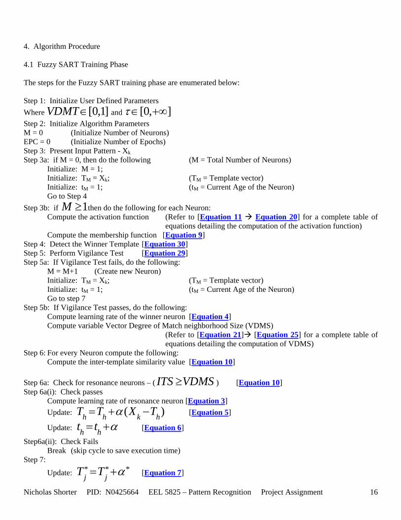
4. Algorithm Procedure 4.1 Fuzzy SART Training Phase The steps for the Fuzzy SART training phase are enumerated below: Step 1: Initialize User Defined Parameters Where and [0,1]VDMT∈ [0, ]τ ∈ +∞ Step 2: Initialize Algorithm Parameters M = 0 (Initialize Number of Neurons) EPC = 0 (Initialize Number of Epochs) Step 3: Present Input Pattern - Xk Step 3a: if M = 0, then do the following (M = Total Number of Neurons) Initialize: M = 1; Initialize: TM = Xk; (TM = Template vector) Initialize: tM = 1; (tM = Current Age of the Neuron) Go to Step 4 Step 3b: if 1M ≥ then do the following for each Neuron:
Compute the activation function (Refer to [Equation 11 Equation 20] for a complete table of equations detailing the computation of the activation function)
Compute the membership function [Equation 9] Step 4: Detect the Winner Template [Equation 30] Step 5: Perform Vigilance Test [Equation 29] Step 5a: If Vigilance Test fails, do the following: M = M+1 (Create new Neuron) Initialize: TM = Xk; (TM = Template vector) Initialize: tM = 1; (tM = Current Age of the Neuron) Go to step 7 Step 5b: If Vigilance Test passes, do the following: Compute learning rate of the winner neuron [Equation 4] Compute variable Vector Degree of Match neighborhood Size (VDMS)
(Refer to [Equation 21] [Equation 25] for a complete table of equations detailing the computation of VDMS)
Step 6: For every Neuron compute the following: Compute the inter-template similarity value [Equation 10] Step 6a: Check for resonance neurons – ( ITS VDMS≥ ) [Equation 10] Step 6a(i): Check passes Compute learning rate of resonance neuron [Equation 3] Update: (h h k hT T X T )α= + − [Equation 5]
Update: h ht t α= + [Equation 6]
Step6a(ii): Check Fails Break (skip cycle to save execution time) Step 7:
Update: * *j jT T *α= + [Equation 7]
Nicholas Shorter PID: N0425664 EEL 5825 – Pattern Recognition Project Assignment 16
Nicholas Shorter PID: N0425664 EEL 5825 – Pattern Recognition Project Assignment 17
* Update: * *j jt t α= + [Equation 8]
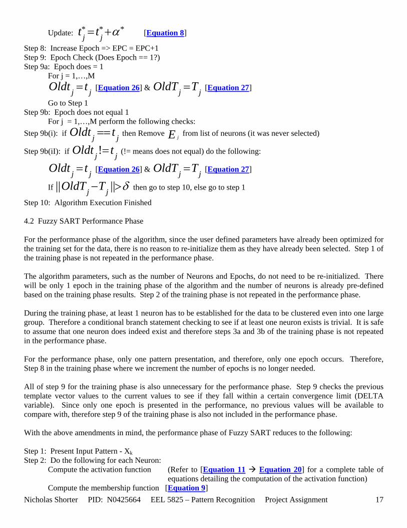
Step 8: Increase Epoch => EPC = EPC+1 Step 9: Epoch Check (Does Epoch == 1?) Step 9a: Epoch does = 1 For j = 1,…,M [Equation 26jOldt t= j ] & jOldT Tj= [Equation 27]
Go to Step 1 Step 9b: Epoch does not equal 1 For j = 1,…,M perform the following checks: Step 9b(i): if then Remove jOldt t== j jE from list of neurons (it was never selected)
Step 9b(iI): if (!= means does not equal) do the following: !jOldt t= j
j [Equation 26jOldt t= ] & jOldT Tj= [Equation 27]
If || ||j jOldT T δ− > then go to step 10, else go to step 1
Step 10: Algorithm Execution Finished 4.2 Fuzzy SART Performance Phase For the performance phase of the algorithm, since the user defined parameters have already been optimized for the training set for the data, there is no reason to re-initialize them as they have already been selected. Step 1 of the training phase is not repeated in the performance phase. The algorithm parameters, such as the number of Neurons and Epochs, do not need to be re-initialized. There will be only 1 epoch in the training phase of the algorithm and the number of neurons is already pre-defined based on the training phase results. Step 2 of the training phase is not repeated in the performance phase. During the training phase, at least 1 neuron has to be established for the data to be clustered even into one large group. Therefore a conditional branch statement checking to see if at least one neuron exists is trivial. It is safe to assume that one neuron does indeed exist and therefore steps 3a and 3b of the training phase is not repeated in the performance phase. For the performance phase, only one pattern presentation, and therefore, only one epoch occurs. Therefore, Step 8 in the training phase where we increment the number of epochs is no longer needed. All of step 9 for the training phase is also unnecessary for the performance phase. Step 9 checks the previous template vector values to the current values to see if they fall within a certain convergence limit (DELTA variable). Since only one epoch is presented in the performance, no previous values will be available to compare with, therefore step 9 of the training phase is also not included in the performance phase. With the above amendments in mind, the performance phase of Fuzzy SART reduces to the following: Step 1: Present Input Pattern - Xk Step 2: Do the following for each Neuron:
Compute the activation function (Refer to [Equation 11 Equation 20] for a complete table of equations detailing the computation of the activation function)
Compute the membership function [Equation 9]
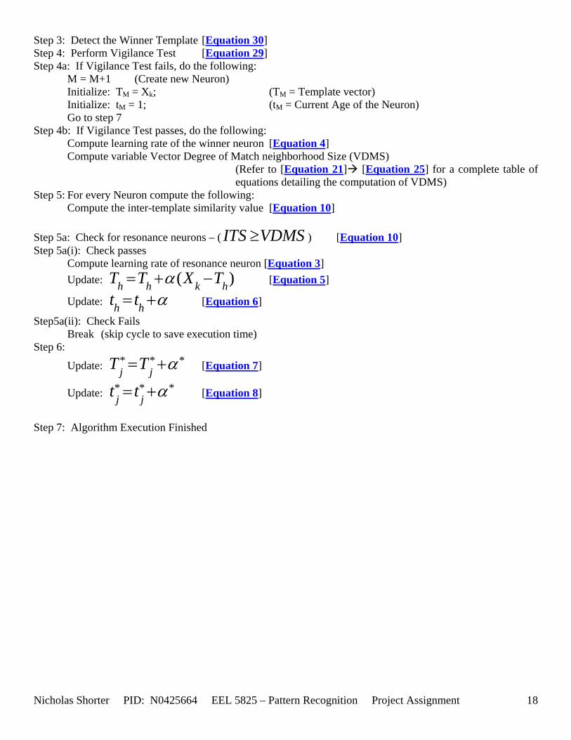
Step 3: Detect the Winner Template [Equation 30] Step 4: Perform Vigilance Test [Equation 29] Step 4a: If Vigilance Test fails, do the following: M = M+1 (Create new Neuron) Initialize: TM = Xk; (TM = Template vector) Initialize: tM = 1; (tM = Current Age of the Neuron) Go to step 7 Step 4b: If Vigilance Test passes, do the following: Compute learning rate of the winner neuron [Equation 4] Compute variable Vector Degree of Match neighborhood Size (VDMS)
(Refer to [Equation 21] [Equation 25] for a complete table of equations detailing the computation of VDMS)
Step 5: For every Neuron compute the following: Compute the inter-template similarity value [Equation 10] Step 5a: Check for resonance neurons – ( ITS VDMS≥ ) [Equation 10] Step 5a(i): Check passes Compute learning rate of resonance neuron [Equation 3] Update: (h h k hT T X T )α= + − [Equation 5]
Update: h ht t α= + [Equation 6]
Step5a(ii): Check Fails Break (skip cycle to save execution time) Step 6:
Update: * *j jT T *α= + [Equation 7]
Update: * *j jt t *α= + [Equation 8]
Step 7: Algorithm Execution Finished
Nicholas Shorter PID: N0425664 EEL 5825 – Pattern Recognition Project Assignment 18
Nicholas Shorter PID: N0425664 EEL 5825 – Pattern Recognition Project Assignment 19
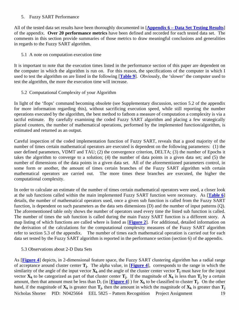
5. Fuzzy SART Performance All of the tested data set results have been thoroughly documented in [Appendix 6 – Data Set Testing Results] of the appendix. Over 20 performance metrics have been defined and recorded for each tested data set. The comments in this section provide summaries of those metrics to draw meaningful conclusions and generalities in regards to the Fuzzy SART algorithm.
5.1 A note on computation execution time It is important to note that the execution times listed in the performance section of this paper are dependent on the computer in which the algorithm is run on. For this reason, the specifications of the computer in which I used to test the algorithm on are listed in the following [Table 9]. Obviously, the ‘slower’ the computer used to test the algorithm, the more the execution time will increase.
5.2 Computational Complexity of your Algorithm In light of the ‘flops’ command becoming obsolete (see Supplementary discussion, section 5.2 of the appendix for more information regarding this), without sacrificing execution speed, while still reporting the number operations executed by the algorithm, the best method to fathom a measure of computation a complexity is via a tactful estimate. By carefully examining the coded Fuzzy SART algorithm and placing a few strategically placed counters, the number of mathematical operations, performed by the implemented function/algorithm, is estimated and returned as an output. Careful inspection of the coded implementation function of Fuzzy SART, reveals that a good majority of the number of times certain mathematical operators are executed is dependent on the following parameters: (1) the user defined parameters, VDMT and TAU; (2) the convergence criterion, DELTA; (3) the number of Epochs it takes the algorithm to converge to a solution; (4) the number of data points in a given data set; and (5) the number of dimensions of the data points in a given data set. All of the aforementioned parameters control, in some form or another, the amount of times certain branches of the Fuzzy SART algorithm with certain mathematical operators are carried out. The more times these branches are executed, the higher the computational complexity. In order to calculate an estimate of the number of times certain mathematical operators were used, a closer look at the sub functions called within the main implemented Fuzzy SART function were necessary. As [Table 6] details, the number of mathematical operators used, once a given sub function is called from the Fuzzy SART function, is dependent on such parameters as the data sets dimensions (D) and the number of input patterns (Q). The aforementioned table only shows the number of operators used every time the listed sub function is called. The number of times the sub function is called during the main Fuzzy SART function is a different story. A map listing of which functions are called where is listed as [Figure 2]. For additional, detailed information on the derivation of the calculations for the computational complexity measures of the Fuzzy SART algorithm refer to section 5.3 of the appendix. The number of times each mathematical operation is carried out for each data set tested by the Fuzzy SART algorithm is reported in the performance section (section 6) of the appendix.
5.3 Observations about 2-D Data Sets As [Figure 4] depicts, in 2-dimensional feature space, the Fuzzy SART clustering algorithm has a radial range of acceptance around cluster center Tj. The alpha value, in [Figure 4], corresponds to the range in which the similarity of the angle of the input vector Xk and the angle of the cluster center vector Tj must have for the input vector Xk to be categorized as part of that cluster center Tj. If the magnitude of Xk is less than Tj by a certain amount, then that amount must be less than D1 (in [Figure 4] ) for Xk to be classified to cluster Tj. On the other hand, if the magnitude of Xk is greater than Tj, then the amount in which the magnitude of Xk is greater than Tj
Nicholas Shorter PID: N0425664 EEL 5825 – Pattern Recognition Project Assignment 20
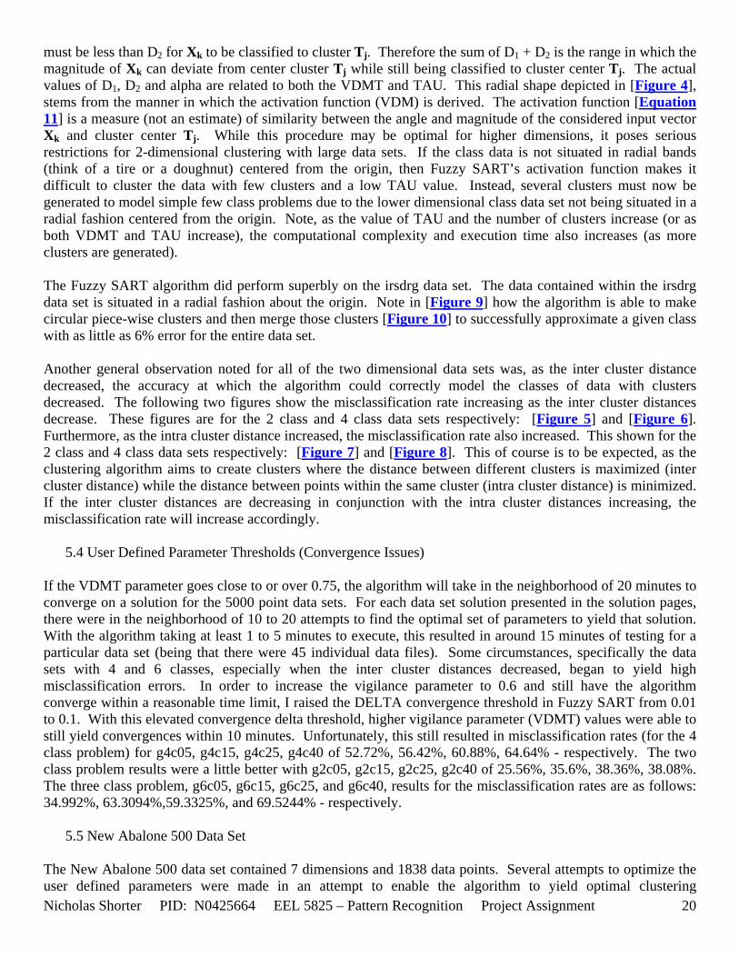
must be less than D2 for Xk to be classified to cluster Tj. Therefore the sum of D1 + D2 is the range in which the magnitude of Xk can deviate from center cluster Tj while still being classified to cluster center Tj. The actual values of D1, D2 and alpha are related to both the VDMT and TAU. This radial shape depicted in [Figure 4], stems from the manner in which the activation function (VDM) is derived. The activation function [Equation 11] is a measure (not an estimate) of similarity between the angle and magnitude of the considered input vector Xk and cluster center Tj. While this procedure may be optimal for higher dimensions, it poses serious restrictions for 2-dimensional clustering with large data sets. If the class data is not situated in radial bands (think of a tire or a doughnut) centered from the origin, then Fuzzy SART’s activation function makes it difficult to cluster the data with few clusters and a low TAU value. Instead, several clusters must now be generated to model simple few class problems due to the lower dimensional class data set not being situated in a radial fashion centered from the origin. Note, as the value of TAU and the number of clusters increase (or as both VDMT and TAU increase), the computational complexity and execution time also increases (as more clusters are generated). The Fuzzy SART algorithm did perform superbly on the irsdrg data set. The data contained within the irsdrg data set is situated in a radial fashion about the origin. Note in [Figure 9] how the algorithm is able to make circular piece-wise clusters and then merge those clusters [Figure 10] to successfully approximate a given class with as little as 6% error for the entire data set. Another general observation noted for all of the two dimensional data sets was, as the inter cluster distance decreased, the accuracy at which the algorithm could correctly model the classes of data with clusters decreased. The following two figures show the misclassification rate increasing as the inter cluster distances decrease. These figures are for the 2 class and 4 class data sets respectively: [Figure 5] and [Figure 6]. Furthermore, as the intra cluster distance increased, the misclassification rate also increased. This shown for the 2 class and 4 class data sets respectively: [Figure 7] and [Figure 8]. This of course is to be expected, as the clustering algorithm aims to create clusters where the distance between different clusters is maximized (inter cluster distance) while the distance between points within the same cluster (intra cluster distance) is minimized. If the inter cluster distances are decreasing in conjunction with the intra cluster distances increasing, the misclassification rate will increase accordingly.
5.4 User Defined Parameter Thresholds (Convergence Issues) If the VDMT parameter goes close to or over 0.75, the algorithm will take in the neighborhood of 20 minutes to converge on a solution for the 5000 point data sets. For each data set solution presented in the solution pages, there were in the neighborhood of 10 to 20 attempts to find the optimal set of parameters to yield that solution. With the algorithm taking at least 1 to 5 minutes to execute, this resulted in around 15 minutes of testing for a particular data set (being that there were 45 individual data files). Some circumstances, specifically the data sets with 4 and 6 classes, especially when the inter cluster distances decreased, began to yield high misclassification errors. In order to increase the vigilance parameter to 0.6 and still have the algorithm converge within a reasonable time limit, I raised the DELTA convergence threshold in Fuzzy SART from 0.01 to 0.1. With this elevated convergence delta threshold, higher vigilance parameter (VDMT) values were able to still yield convergences within 10 minutes. Unfortunately, this still resulted in misclassification rates (for the 4 class problem) for g4c05, g4c15, g4c25, g4c40 of 52.72%, 56.42%, 60.88%, 64.64% - respectively. The two class problem results were a little better with g2c05, g2c15, g2c25, g2c40 of 25.56%, 35.6%, 38.36%, 38.08%. The three class problem, g6c05, g6c15, g6c25, and g6c40, results for the misclassification rates are as follows: 34.992%, 63.3094%,59.3325%, and 69.5244% - respectively.
5.5 New Abalone 500 Data Set The New Abalone 500 data set contained 7 dimensions and 1838 data points. Several attempts to optimize the user defined parameters were made in an attempt to enable the algorithm to yield optimal clustering
Nicholas Shorter PID: N0425664 EEL 5825 – Pattern Recognition Project Assignment 21
performance. The various attempts at differing parameters are detailed in [Table 10]. The algorithm’s training phase did not perform so well, only returning with a ~56% accuracy rate on the training data. The algorithm’s performance on unforeseen data was even worse with only a ~32% accuracy rate on correctly clustering the data. This poor performance could be due to several factors: (1) complex hyper-dimensional class shapes; (2) Fuzzy SART not having enough clusters to model the data; (3) the delta parameter being to low (preventing reasonable convergence times); (4) the user parameters being ill-defined. As mentioned above, increasing both TAU and the VDMT parameter beyond 50 and .7 respectively, drive the computation for the data set to at least 20 minutes. Therefore, to reasonably test the data set, only a finite number of clusters and epochs were feasible – which unfortunately resulted in poorer performance.
5.6 Nick Generated Data Set and execution times The data that was provided as an easy, clear to comprehend, example of the algorithm’s working nature was created by generating points of a uniform random distribution about a specified set of cluster center points. The name of the MATLAB file used to generate this example/sample data was ‘datatest.m’ In order to make the initial test data set simple, the average inter cluster distances were set reasonable far apart from one another (0.31932) while keeping the average intra cluster distances small. The size of the data set was also limited to only 1000 points to keep the convergence times for large values of VDMT to a reasonable minimum. The clustering algorithm performed flawlessly on the test data set clustering the data with 100% accuracy. The following figures [Figure 12] and [Figure 13] show the clusters generated and then the merging of the clusters to match the original class labels. As one can see from the aforementioned figures, the classes are generated reasonably far from one another ensuring an easy match for the algorithm and therefore simple check to the algorithm’s working nature. The execution time for this 1000 point, 2 dimensional data set was 36.219 seconds for the training phase and 3.437 seconds for the performance phase. After witnessing the algorithm perform flawlessly on 1000 data points relatively far apart, I then decided to push those points close together, but in turn also reduce the number of data points. In the second set of generated data points, the total number of points is now only a mere 50. However, with such a significant reduction in the data size, a larger number of epochs now converges within an exponentially smaller time frame. An original plot of the performance data [Figure 14] and a final plot of the clustered data [Figure 15] have been documented accordingly. Fuzzy SART clustered this generated data set with ~83% accuracy. Four additional data sets were generated (their results not shown in the appendix) and the user parameters were modified to keep the number of Epochs approximately the same for each test. The purpose of this was to hold the number of epochs constant, while increasing the size of the data set to see how this would affect the amount of time it would take the algorithm to converge to a solution. If the user parameters were modified such that the algorithm would run 15 epochs for all 4 generated test sets, as the training size increased, the execution time increased exponentially [Figure 16]. The table of data corresponding to the previous figure is listed as follows – [Table 11]. Finally, 1 additional data set (quantitative metric reports included in appendix as generated 1 and then generated 1 w/ random) was tested twice by Fuzzy SART. The first test was routine, the second test however, the following lines of code were added to the beginning of the proj_gr.m file (used to generate the data set twice) to randomize the input order for the second test: RAWINPUTt = data_nick; %Testing Data RAWINPUTt = rmrw(data_nick); RAWINPUTp = data_nickp; %Performance Data RAWINPUTp = rmrw(data_nickp);
Nicholas Shorter PID: N0425664 EEL 5825 – Pattern Recognition Project Assignment 22
The “RAWINPUT” data variables are what’s fed into the Fuzzy SART function. The rmrw function is as follows: function [Rmz] = rmrw(Input); [R,C] = size(Input); %Extracting Dimensions of Input Matrix rnd = rand(R,1); %Creating random array equal to rows of input matrix [S,I] = sort(rnd); %Creating index array to structure new randomized matrix with Rmz = Input(I,:); %Structuring new matrix with randomized rows The rmrw function takes its input and randomizes the row order and returns the inputted matrix with the randomized rows. This exercise was used to test whether or not Fuzzy SART’s performance was dependent on the input order. For both sets of tested data, the exact same number of mathematical operators was executed. Furthermore, the exact same number of clusters was created in the same number of epochs with very close execution times (times will differ slightly based on other processes currently being handled by computer). In addition to these equivalents, the exact same classification rates were realized. Fuzzy SART does indeed perform completely independent of the order of the input data.
5.7 Pageblocks Data Set The Fuzzy SART algorithm for high values of TAU and VDMT would not converge to a solution for this data set. Again, I raised the DELTA convergence parameter to reduce the convergence wait. Then I lowered TAU and VDMT to attempt to get reasonable convergence times for this data set. The algorithm then converged quite quickly with remarkable accuracy. For the pageblocks data set, Fuzzy SART was able to model the classes with clusters with a 92% accuracy on the performance set! Furthermore, the algorithm was able to do this only in 4 epochs and with 4 clusters. Conclusions: From the tests performed above, several strengths and weaknesses can be formulated based on the algorithm’s performance against the various different types of test sets: Observations:
1. Fuzzy SART performs better on data sets where the class centers are far apart from one another in conjunction with the class data points being located close to the class center
Strengths:
1. Fuzzy SART performs excellently on 2-D data sets that are situated in a radial fashion with respect to the origin (iris data set)
2. Fuzzy SART only has 2 user defined parameters – both of which contain physical intuitive meanings 3. Fuzzy SART requires no a priori knowledge of the data set 4. Fuzzy SART exhibits stability for small changes in the input parameters 5. The number of clusters and how Fuzzy SART clusters data is independent of the order in which the data
is presented to the algorithm 6. No pre-processing of the input data is necessary for Fuzzy SART
Weaknesses:
1. Aside from the 2 user defined parameters, Fuzzy SART does not provide a means for incorporating a priori knowledge (i.e. cluster centers)
2. Fuzzy SART (in the case of the 2,4, and 6 class problems) has issues with modeling circular clusters with small inter cluster distances and large intra cluster distances
3. Fuzzy SART’s computational complexity for large scale data sets, in some instances, can make attaining certain cluster accuracies unfeasible with over bearing calculation times

Nicholas Shorter PID: N0425664 EEL 5825 – Pattern Recognition Project Assignment 23
4. Fuzzy SART’s native clustering shapes (especially when TAU is really low) tends to lean towards arcs or radial bands with center of circumference being the origin (see [Figure 11] for a pictorial example).
For moderately sized data sets (around 2000 data points and below), Fuzzy SART performs moderately, given that the intra cluster distances for given classes are small and inter cluster distances are large. As the intra cluster distances decrease and inter cluster distances increase, the number of clusters needed to model the classes, and therefore computational complexity of the algorithm increases. For large data sets, this increase can sometimes result in convergence times greater than half an hour. One workaround to this issue would be to uniformly sample the large scale data set and base the calculations off of a smaller subset. However, this results in a loss of information and presents further complications when testing on unforeseen data. When given the time to converge however, the algorithm delivers excellent results, having the ability to cluster both low and high dimensional data sets. For the computational complexity issue, the algorithm compromises by offering several perks listed in the above strengths section. One perk in particular is its user parameters being limited to only 2 with both having physical intuitive meanings. For this particular application of Fuzzy SART for this project, the trade off accuracy for computational complexity is quite evident. The algorithm, in some circumstances, needs large amounts of time to deliver the demanded performance. The algorithm will find a solution; the engineering comes in minimizing the time to get to that solution and ensuring that the solution is indeed a desirable one.

Nicholas Shorter PID: N0425664 EEL 5825 – Pattern Recognition Project Assignment 24
Appendix
Appendix
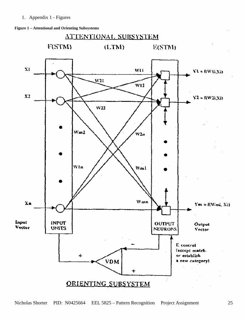
1. Appendix 1 - Figures Figure 1 – Attentional and Orienting Subsystems
Nicholas Shorter PID: N0425664 EEL 5825 – Pattern Recognition Project Assignment 25
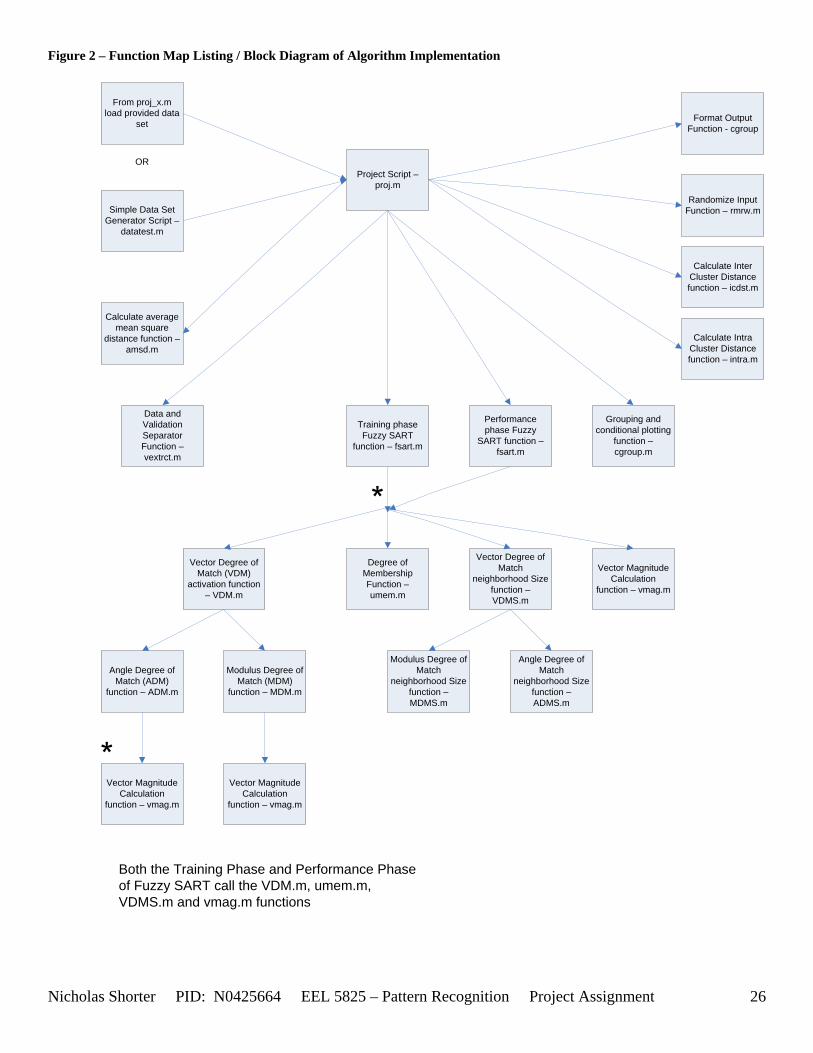
Figure 2 – Function Map Listing / Block Diagram of Algorithm Implementation
Project Script –proj.m
Data and Validation Separator Function –vextrct.m
Simple Data Set Generator Script –
datatest.m
Training phase Fuzzy SART
function – fsart.m
Vector Degree of Match (VDM)
activation function – VDM.m
Modulus Degree of Match (MDM)
function – MDM.m
Angle Degree of Match (ADM)
function – ADM.m
Degree of Membership Function –umem.m
Vector Degree of Match
neighborhood Size function –VDMS.m
Vector Magnitude Calculation
function – vmag.m
Vector Magnitude Calculation
function – vmag.m
Vector Magnitude Calculation
function – vmag.m
Performance phase Fuzzy
SART function –fsart.m
Modulus Degree of Match
neighborhood Size function –MDMS.m
Angle Degree of Match
neighborhood Size function –ADMS.m
Both the Training Phase and Performance Phase of Fuzzy SART call the VDM.m, umem.m, VDMS.m and vmag.m functions
Grouping and conditional plotting
function –cgroup.m
From proj_x.m load provided data
set
OR
Randomize Input Function – rmrw.m
Format Output Function - cgroup
Calculate Inter Cluster Distance function – icdst.m
Calculate Intra Cluster Distance function – intra.m
Calculate average mean square
distance function –amsd.m
Nicholas Shorter PID: N0425664 EEL 5825 – Pattern Recognition Project Assignment 26
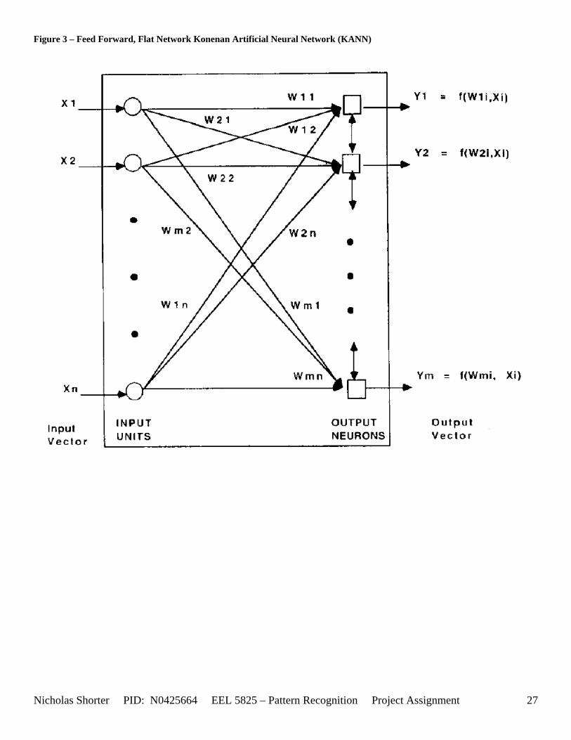
Figure 3 – Feed Forward, Flat Network Konenan Artificial Neural Network (KANN)
Nicholas Shorter PID: N0425664 EEL 5825 – Pattern Recognition Project Assignment 27
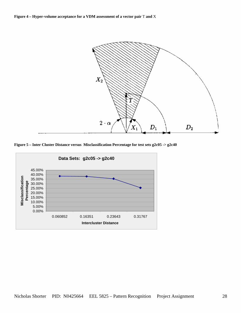
Figure 4 – Hyper-volume acceptance for a VDM assessment of a vector pair T and X
Figure 5 – Inter Cluster Distance versus Misclassification Percentage for test sets g2c05 -> g2c40
Data Sets: g2c05 -> g2c40
0.00%5.00%
10.00%15.00%20.00%25.00%30.00%35.00%40.00%45.00%
0.060852 0.16351 0.23643 0.31767
Intercluster Distance
Mis
clas
sific
atio
n Pe
rcen
tage
Nicholas Shorter PID: N0425664 EEL 5825 – Pattern Recognition Project Assignment 28
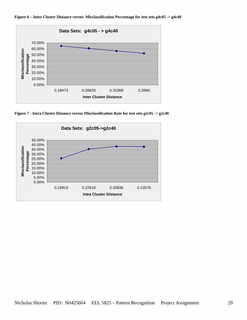
Figure 6 – Inter Cluster Distance versus Misclassification Percentage for test sets g4c05 -> g4c40
Data Sets: g4c05 - > g4c40
0.00%10.00%20.00%30.00%40.00%50.00%60.00%70.00%
0.18473 0.26626 0.31968 0.3966
Inter Cluster Distance
Mis
clas
sific
atio
n Pe
rcen
tage
Figure 7 - Intra Cluster Distance versus Misclassification Rate for test sets g2c05 -> g2c40
Data Sets: g2c05->g2c40
0.00%5.00%
10.00%15.00%20.00%25.00%30.00%35.00%40.00%45.00%
0.19919 0.22818 0.20836 0.23576
Intra Cluster Distance
Mis
clas
sific
atio
n Pe
rcen
tage
Nicholas Shorter PID: N0425664 EEL 5825 – Pattern Recognition Project Assignment 29
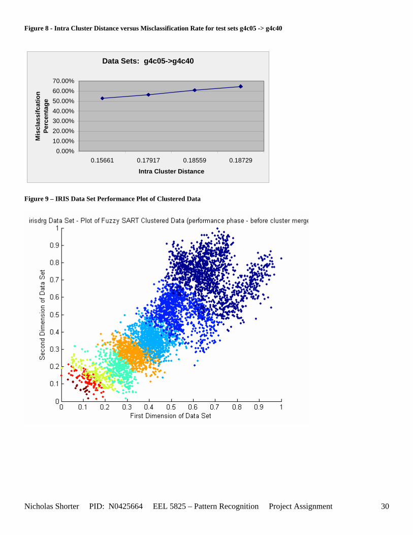
Figure 8 - Intra Cluster Distance versus Misclassification Rate for test sets g4c05 -> g4c40
Data Sets: g4c05->g4c40
0.00%10.00%20.00%30.00%40.00%50.00%60.00%70.00%
0.15661 0.17917 0.18559 0.18729
Intra Cluster Distance
Mis
clas
sifc
atio
n Pe
rcen
tage
Figure 9 – IRIS Data Set Performance Plot of Clustered Data
Nicholas Shorter PID: N0425664 EEL 5825 – Pattern Recognition Project Assignment 30
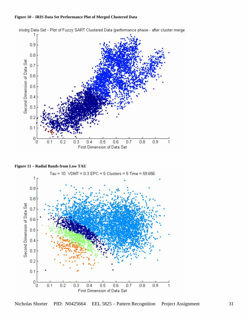
Figure 10 – IRIS Data Set Performance Plot of Merged Clustered Data
Figure 11 – Radial Bands from Low TAU
Nicholas Shorter PID: N0425664 EEL 5825 – Pattern Recognition Project Assignment 31
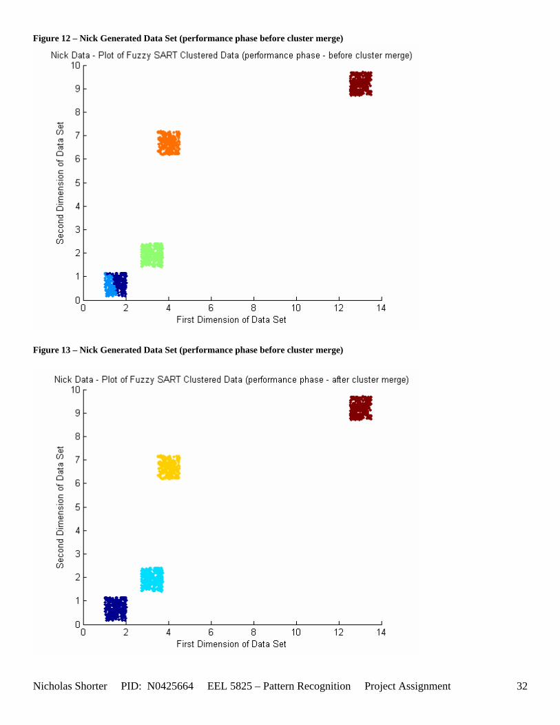
Figure 12 – Nick Generated Data Set (performance phase before cluster merge)
Figure 13 – Nick Generated Data Set (performance phase before cluster merge)
Nicholas Shorter PID: N0425664 EEL 5825 – Pattern Recognition Project Assignment 32
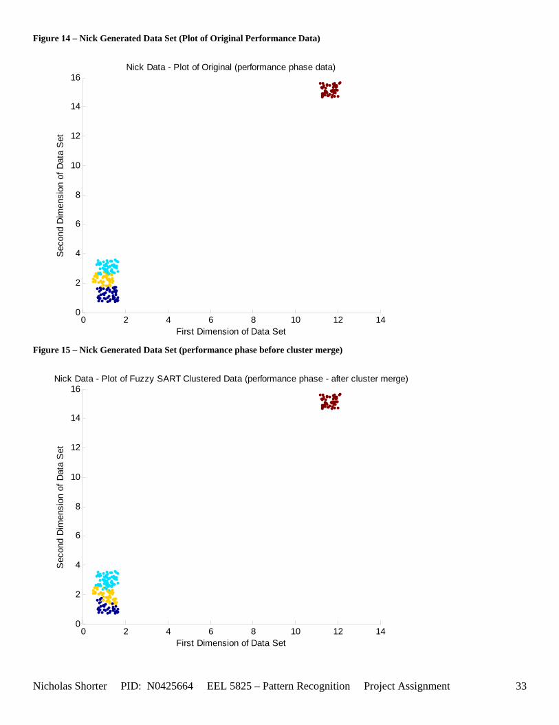
Figure 14 – Nick Generated Data Set (Plot of Original Performance Data)
0 2 4 6 8 10 12 140
2
4
6
8
10
12
14
16Nick Data - Plot of Original (performance phase data)
First Dimension of Data Set
Sec
ond
Dim
ensi
on o
f Dat
a S
et
Figure 15 – Nick Generated Data Set (performance phase before cluster merge)
0 2 4 6 8 10 12 140
2
4
6
8
10
12
14
16Nick Data - Plot of Fuzzy SART Clustered Data (performance phase - after cluster merge)
First Dimension of Data Set
Sec
ond
Dim
ensi
on o
f Dat
a S
et
Nicholas Shorter PID: N0425664 EEL 5825 – Pattern Recognition Project Assignment 33
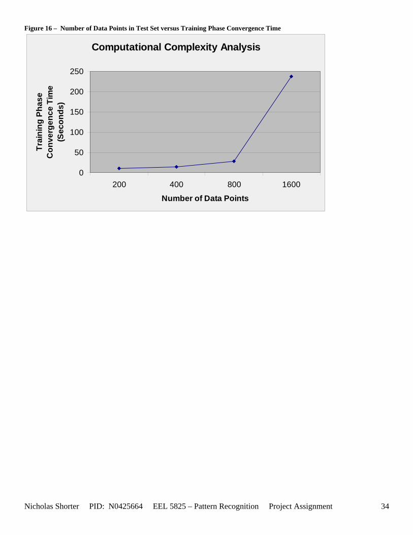
Figure 16 – Number of Data Points in Test Set versus Training Phase Convergence Time
Computational Complexity Analysis
0
50
100
150
200
250
200 400 800 1600
Number of Data Points
Trai
ning
Pha
se
Con
verg
ence
Tim
e (S
econ
ds)
Nicholas Shorter PID: N0425664 EEL 5825 – Pattern Recognition Project Assignment 34
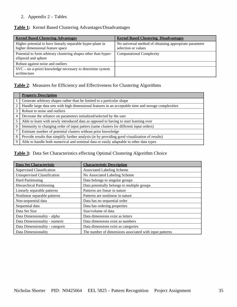
Nicholas Shorter PID: N0425664 EEL 5825 – Pattern Recognition Project Assignment 35
2. Appendix 2 – Tables Table 1: Kernel Based Clustering Advantages/Disadvantages Kernel Based Clustering Advantages Kernel Based Clustering Disadvantages Higher potential to have linearly separable hyper-plane in higher dimensional feature space
No universal method of obtaining appropriate parameter selection or values
Potential to form arbitrary clustering shapes other than hyper-ellipsoid and sphere
Computational Complexity
Robust against noise and outliers SVC – no a-priori knowledge necessary to determine system architecture
Table 2: Measures for Efficiency and Effectiveness for Clustering Algorithms Property Description 1 Generate arbitrary shapes rather than be limited to a particular shape 2 Handle large data sets with high dimensional features in an acceptable time and storage complexities 3 Robust to noise and outliers 4 Decrease the reliance on parameters initialized/selected by the user 5 Able to learn with newly introduced data as opposed to having to start learning over 6 Immunity to changing order of input patters (same clusters for different input orders) 7 Estimate number of potential clusters without prior knowledge 8 Provide results that simplify further analysis (ie by providing good visualization of results) 9 Able to handle both numerical and nominal data or easily adaptable to other data types
Table 3: Data Set Characteristics effecting Optimal Clustering Algorithm Choice Data Set Characteristic Characteristic Description Supervised Classification Associated Labeling Scheme Unsupervised Classification No Associated Labeling Scheme Hard Partitioning Data belongs to singular groups Hierarchical Partitioning Data potentially belongs to multiple groups Linearly separable patterns Patterns are linear in nature Nonlinear separable patterns Patterns are nonlinear in nature Non-sequential data Data has no sequential order Sequential data Data has ordering properties Data Set Size Size/volume of data Data Dimensionality - alpha Data dimensions exist as letters Data Dimensionality - numeric Data dimensions exist as numbers Data Dimensionality - categoric Data dimensions exist as categories Data Dimensionality The number of dimensions associated with input patterns
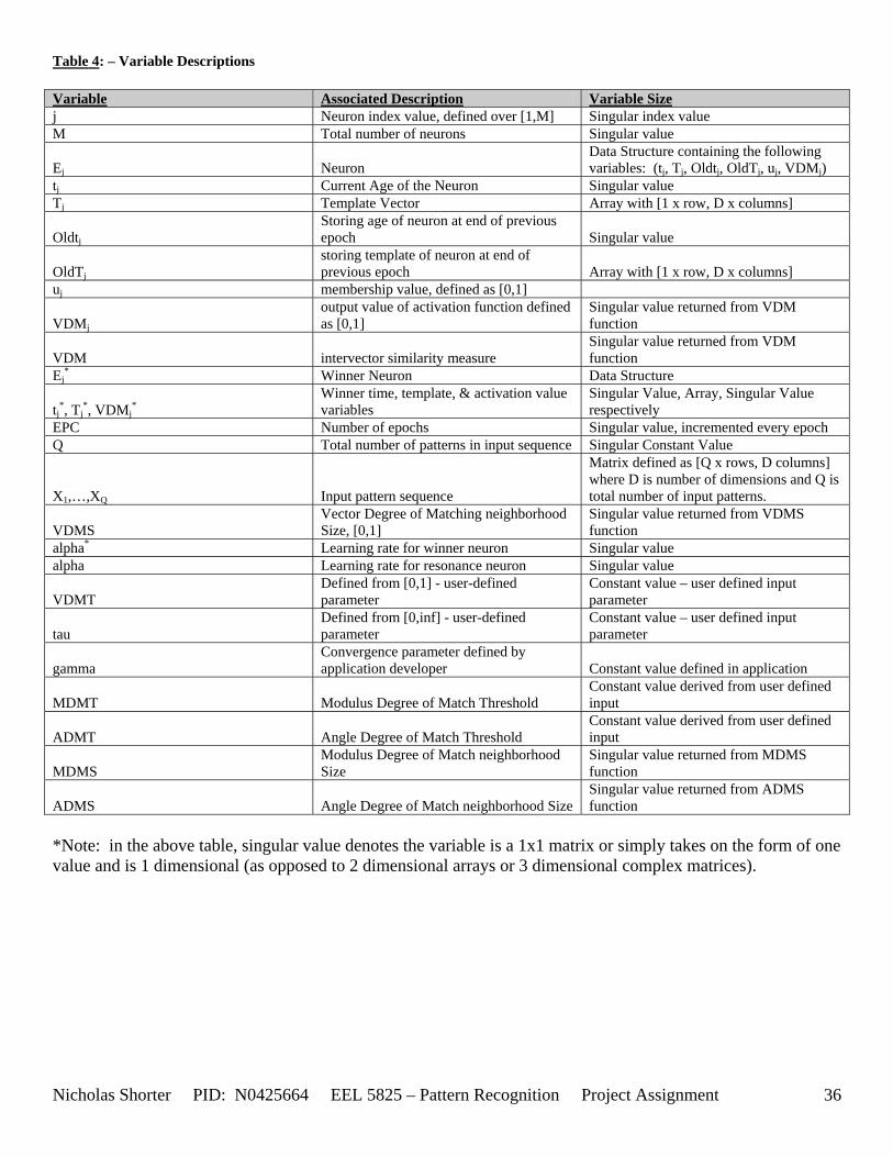
Nicholas Shorter PID: N0425664 EEL 5825 – Pattern Recognition Project Assignment 36
Table 4: – Variable Descriptions Variable Associated Description Variable Size j Neuron index value, defined over [1,M] Singular index value M Total number of neurons Singular value
Ej Neuron Data Structure containing the following variables: (tj, Tj, Oldtj, OldTj, uj, VDMj)
tj Current Age of the Neuron Singular value Tj Template Vector Array with [1 x row, D x columns]
Oldtj Storing age of neuron at end of previous epoch Singular value
OldTj storing template of neuron at end of previous epoch Array with [1 x row, D x columns]
uj membership value, defined as [0,1]
VDMj output value of activation function defined as [0,1]
Singular value returned from VDM function
VDM intervector similarity measure Singular value returned from VDM function
Ej* Winner Neuron Data Structure
tj*, Tj
*, VDMj*
Winner time, template, & activation value variables
Singular Value, Array, Singular Value respectively
EPC Number of epochs Singular value, incremented every epoch Q Total number of patterns in input sequence Singular Constant Value
X1,…,XQ Input pattern sequence
Matrix defined as [Q x rows, D columns] where D is number of dimensions and Q is total number of input patterns.
VDMS Vector Degree of Matching neighborhood Size, [0,1]
Singular value returned from VDMS function
alpha* Learning rate for winner neuron Singular value alpha Learning rate for resonance neuron Singular value
VDMT Defined from [0,1] - user-defined parameter
Constant value – user defined input parameter
tau Defined from [0,inf] - user-defined parameter
Constant value – user defined input parameter
gamma Convergence parameter defined by application developer Constant value defined in application
MDMT Modulus Degree of Match Threshold Constant value derived from user defined input
ADMT Angle Degree of Match Threshold Constant value derived from user defined input
MDMS Modulus Degree of Match neighborhood Size
Singular value returned from MDMS function
ADMS Angle Degree of Match neighborhood Size Singular value returned from ADMS function
*Note: in the above table, singular value denotes the variable is a 1x1 matrix or simply takes on the form of one value and is 1 dimensional (as opposed to 2 dimensional arrays or 3 dimensional complex matrices).
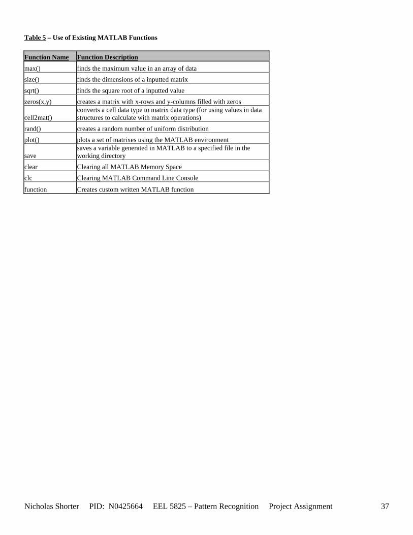
Nicholas Shorter PID: N0425664 EEL 5825 – Pattern Recognition Project Assignment 37
Table 5 – Use of Existing MATLAB Functions Function Name Function Description
max() finds the maximum value in an array of data size() finds the dimensions of a inputted matrix
sqrt() finds the square root of a inputted value zeros(x,y) creates a matrix with x-rows and y-columns filled with zeros
cell2mat() converts a cell data type to matrix data type (for using values in data structures to calculate with matrix operations)
rand() creates a random number of uniform distribution
plot() plots a set of matrixes using the MATLAB environment
save saves a variable generated in MATLAB to a specified file in the working directory
clear Clearing all MATLAB Memory Space
clc Clearing MATLAB Command Line Console
function Creates custom written MATLAB function
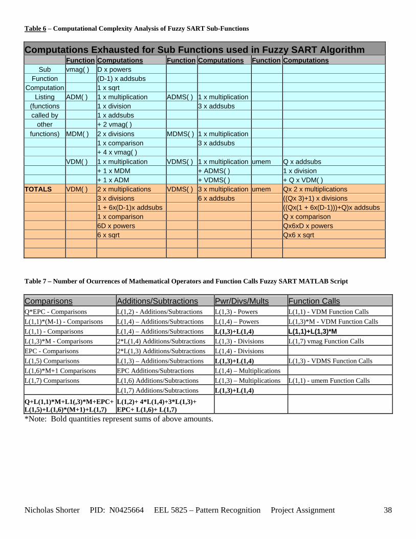
Nicholas Shorter PID: N0425664 EEL 5825 – Pattern Recognition Project Assignment 38
Table 6 – Computational Complexity Analysis of Fuzzy SART Sub-Functions Computations Exhausted for Sub Functions used in Fuzzy SART Algorithm Function Computations Function Computations Function Computations
Sub vmag( ) D x powers Function (D-1) x addsubs
Computation 1 x sqrt Listing ADM( ) 1 x multiplication ADMS( ) 1 x multiplication
(functions 1 x division 3 x addsubs called by 1 x addsubs
other + 2 vmag( ) functions) MDM( ) 2 x divisions MDMS( ) 1 x multiplication
1 x comparison 3 x addsubs + 4 x vmag( ) VDM( ) 1 x multiplication VDMS( ) 1 x multiplication umem Q x addsubs + 1 x MDM + ADMS( ) 1 x division + 1 x ADM + VDMS( ) + Q x VDM( )
TOTALS VDM( ) 2 x multiplications VDMS( ) 3 x multiplication umem Qx 2 x multiplications 3 x divisions 6 x addsubs ((Qx 3)+1) x divisions 1 + 6x(D-1)x addsubs ((Qx(1 + 6x(D-1)))+Q)x addsubs 1 x comparison Q x comparison 6D x powers Qx6xD x powers 6 x sqrt Qx6 x sqrt Table 7 – Number of Ocurrences of Mathematical Operators and Function Calls Fuzzy SART MATLAB Script Comparisons Additions/Subtractions Pwr/Divs/Mults Function Calls Q*EPC - Comparisons L(1,2) - Additions/Subtractions L(1,3) - Powers L(1,1) - VDM Function Calls L(1,1)*(M-1) - Comparisons L(1,4) – Additions/Subtractions L(1,4) – Powers L(1,3)*M - VDM Function Calls L(1,1) - Comparisons L(1,4) – Additions/Subtractions L(1,3)+L(1,4) L(1,1)+L(1,3)*M L(1,3)*M - Comparisons 2*L(1,4) Additions/Subtractions L(1,3) - Divisions L(1,7) vmag Function Calls EPC - Comparisons 2*L(1,3) Additions/Subtractions L(1,4) - Divisions L(1,5) Comparisons L(1,3) – Additions/Subtractions L(1,3)+L(1,4) L(1,3) - VDMS Function Calls L(1,6)*M+1 Comparisons EPC Additions/Subtractions L(1,4) – Multiplications L(1,7) Comparisons L(1,6) Additions/Subtractions L(1,3) – Multiplications L(1,1) - umem Function Calls L(1,7) Additions/Subtractions L(1,3)+L(1,4) Q+L(1,1)*M+L1(,3)*M+EPC+L(1,5)+L(1,6)*(M+1)+L(1,7)
L(1,2)+ 4*L(1,4)+3*L(1,3)+ EPC+ L(1,6)+ L(1,7)
*Note: Bold quantities represent sums of above amounts.
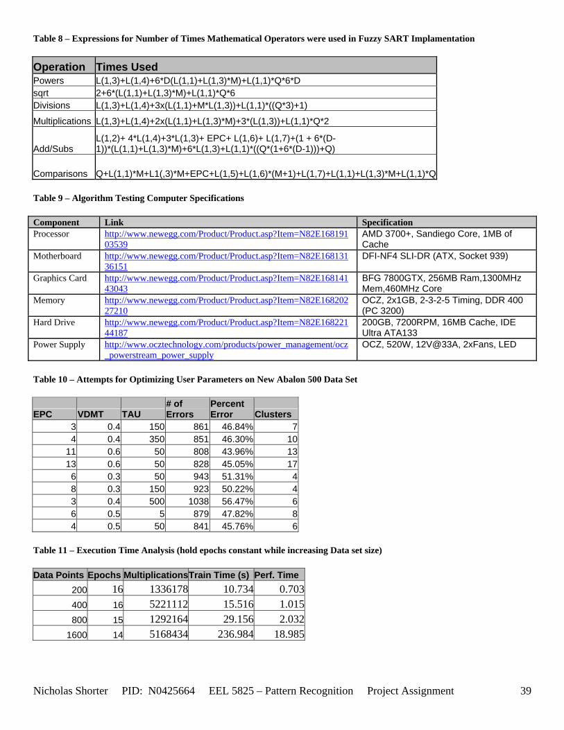
Nicholas Shorter PID: N0425664 EEL 5825 – Pattern Recognition Project Assignment 39
Table 8 – Expressions for Number of Times Mathematical Operators were used in Fuzzy SART Implamentation Operation Times Used Powers L(1,3)+L(1,4)+6*D(L(1,1)+L(1,3)*M)+L(1,1)*Q*6*D sqrt 2+6*(L(1,1)+L(1,3)*M)+L(1,1)*Q*6 Divisions L(1,3)+L(1,4)+3x(L(1,1)+M*L(1,3))+L(1,1)*((Q*3)+1)
Multiplications L(1,3)+L(1,4)+2x(L(1,1)+L(1,3)*M)+3*(L(1,3))+L(1,1)*Q*2
Add/Subs L(1,2)+ 4*L(1,4)+3*L(1,3)+ EPC+ L(1,6)+ L(1,7)+(1 + 6*(D-1))*(L(1,1)+L(1,3)*M)+6*L(1,3)+L(1,1)*((Q*(1+6*(D-1)))+Q)
Comparisons Q+L(1,1)*M+L1(,3)*M+EPC+L(1,5)+L(1,6)*(M+1)+L(1,7)+L(1,1)+L(1,3)*M+L(1,1)*Q Table 9 – Algorithm Testing Computer Specifications Component Link Specification Processor http://www.newegg.com/Product/Product.asp?Item=N82E168191
03539AMD 3700+, Sandiego Core, 1MB of Cache
Motherboard http://www.newegg.com/Product/Product.asp?Item=N82E16813136151
DFI-NF4 SLI-DR (ATX, Socket 939)
Graphics Card http://www.newegg.com/Product/Product.asp?Item=N82E16814143043
BFG 7800GTX, 256MB Ram,1300MHz Mem,460MHz Core
Memory http://www.newegg.com/Product/Product.asp?Item=N82E16820227210
OCZ, 2x1GB, 2-3-2-5 Timing, DDR 400 (PC 3200)
Hard Drive http://www.newegg.com/Product/Product.asp?Item=N82E16822144187
200GB, 7200RPM, 16MB Cache, IDE Ultra ATA133
Power Supply http://www.ocztechnology.com/products/power_management/ocz_powerstream_power_supply
OCZ, 520W, 12V@33A, 2xFans, LED
Table 10 – Attempts for Optimizing User Parameters on New Abalon 500 Data Set
EPC VDMT TAU # of Errors
Percent Error Clusters
3 0.4 150 861 46.84% 74 0.4 350 851 46.30% 10
11 0.6 50 808 43.96% 1313 0.6 50 828 45.05% 17
6 0.3 50 943 51.31% 48 0.3 150 923 50.22% 43 0.4 500 1038 56.47% 66 0.5 5 879 47.82% 84 0.5 50 841 45.76% 6
Table 11 – Execution Time Analysis (hold epochs constant while increasing Data set size) Data Points Epochs Multiplications Train Time (s) Perf. Time
200 16 1336178 10.734 0.703400 16 5221112 15.516 1.015800 15 1292164 29.156 2.032
1600 14 5168434 236.984 18.985

3. Appendix 3 – Equations Performance Measures Equations: Equation Equation Caption
J
1
Nc
j 1
Sj
x
x⎯
mj⎯
−( )2∑=
∑=
Where: Nc: the number of clusters that were created x: A data point from your data set mj: The jth cluster center Sj: the set of data points that belong the jth cluster
Equation 1 - Mean Squared Distance
D2 x1( ) x2( ),⎡⎣ ⎤⎦⎡⎣ ⎤⎦⎯
1k k 1−( )⋅
1
k
j 1
k
i 1
n
k
xkj xk
i−⎛
⎝⎞⎠
2
∑=
∑=
∑=
⋅
Equation 2 – Intra Cluster Distance
Learning Rates for Fuzzy SART: Equation Equation Caption
*[( ) )]*( , , ) t th jh h j ju t t u τ
α α+
= =
Equation 3 – Learning Rate of Resonance Neuron
** * * *( , ) j
j j jtu t u τ
α α= =
Equation 4 – Learning Rate of winning Neuron
Update Equations for Fuzzy SART: Equation Equation Caption
( )h h k hT T X Tα= + − Equation 5 – Update Equation for Template Vector
h ht t α= + Equation 6 – Update Equation for age of neuron variable
* *j jT T *α= +
Equation 7 – Update Equation for Winning Neuron Template Vector
* *j jt t *α= +
Equation 8 – Update Equation for Winning Neuron, age of neuron variable
Membership Equation: Equation Equation Caption
1 1
( , )( , , , 1,..., )
( , )
j j kj k j p M M
p p kp p
VDM VDM T Xu X T T p Mu
VDM VDM T X= = = =
= =∑ ∑
Equation 9 – Membership function
Nicholas Shorter PID: N0425664 EEL 5825 – Pattern Recognition Project Assignment 40
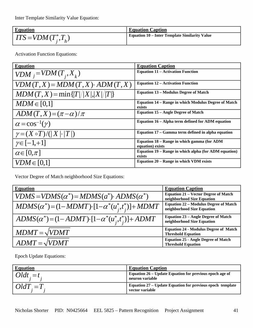
Inter Template Similarity Value Equation: Equation Equation Caption
*( , )j hITS VDM T T= Equation 10 – Inter Template Similarity Value
Activation Function Equations: Equation Equation Caption
( , )j j kVDM T XVDM = Equation 11 – Activation Function
( , ) ( , ) ( , )VDM T X MDM T X ADM T X= ⋅ Equation 12 – Activation Function
( , ) min{| | | |,| | | |}MDM T X T X X T= Equation 13 – Modulus Degree of Match
[0,1]MDM ∈ Equation 14 – Range in which Modulus Degree of Match exists
( , ) ( ) /ADM T X π α π= − Equation 15 – Angle Degree of Match
1cos ( )α γ−= Equation 16 – Alpha term defined for ADM equation
( ) /(| | | |)X T X Tγ = ⋅ Equation 17 – Gamma term defined in alpha equation
[ 1, 1]γ ∈ − + Equation 18 – Range in which gamma (for ADM equation) exists
[0, ]α π∈ Equation 19 – Range in which alpha (for ADM equation) exists
[0,1]VDM∈ Equation 20 – Range in which VDM exists
Vector Degree of Match neighborhood Size Equations: Equation Equation Caption
* * *( ) ( ) ( )VDMS VDMS MDMS a ADMSα α= = ⋅ Equation 21 – Vector Degree of Match neighborhood Size Equation
* * * *( ) (1 ) [1 ( , )]j jMDMS MDMT u t MDMTα α= − ⋅ − + Equation 22 – Modulus Degree of Match neighborhood Size Equation
* * * *( ) (1 ) [1 ( , )]j jADMS ADMT u t ADMTα α= − ⋅ − + Equation 23 – Angle Degree of Match neighborhood Size Equation
MDMT VDMT= Equation 24 - Modulus Degree of Match Threshold Equation
ADMT VDMT= Equation 25 - Angle Degree of Match Threshold Equation
Epoch Update Equations: Equation Equation Caption
j jOldt t= Equation 26 – Update Equation for previous epoch age of neuron variable
j jOldT T= Equation 27 – Update Equation for previous epoch template vector variable
Nicholas Shorter PID: N0425664 EEL 5825 – Pattern Recognition Project Assignment 41
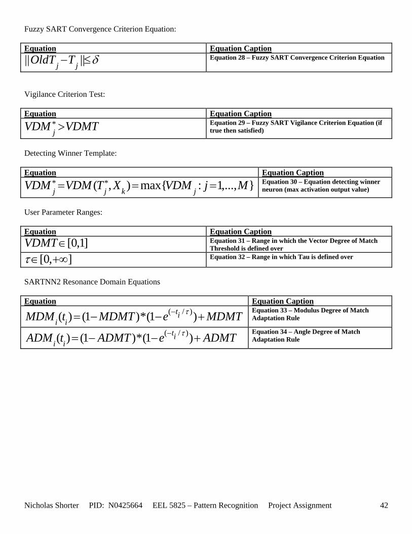
Fuzzy SART Convergence Criterion Equation: Equation Equation Caption || ||j jOldT T δ− ≤ Equation 28 – Fuzzy SART Convergence Criterion Equation
Vigilance Criterion Test: Equation Equation Caption
*jVDM VDMT>
Equation 29 – Fuzzy SART Vigilance Criterion Equation (if true then satisfied)
Detecting Winner Template: Equation Equation Caption
* *( , ) max{ : 1,..., }j j k jVDM VDM T X VDM j M= = = Equation 30 – Equation detecting winner neuron (max activation output value)
User Parameter Ranges: Equation Equation Caption
[0,1]VDMT∈ Equation 31 – Range in which the Vector Degree of Match Threshold is defined over
[0, ]τ∈ +∞ Equation 32 – Range in which Tau is defined over
SARTNN2 Resonance Domain Equations Equation Equation Caption
( / )( ) (1 )*(1 )tii iMDM t MDMT e MDMTτ−= − − +
Equation 33 – Modulus Degree of Match Adaptation Rule
( / )( ) (1 )*(1 )tii iADM t ADMT e ADMTτ−= − − +
Equation 34 – Angle Degree of Match Adaptation Rule
Nicholas Shorter PID: N0425664 EEL 5825 – Pattern Recognition Project Assignment 42

Nicholas Shorter PID: N0425664 EEL 5825 – Pattern Recognition Project Assignment 43
4. Appendix 4 – Original Directions
EEL 5825 EEL 5825 Project Assignment
Due December 9, 2005
1. Study the papers in the in the reference list provided. They are both survey papers on clustering methods. 2. Provide a detailed summary of one of these papers. The summary should include an Intro, a Main Part,
Conclusions, Own impression of Paper Usefulness, and a shortened list of references. 3. Using the review papers or other clustering references (e.g., Tou and Gonzalez, Duda and Hart, others) define
quantitative measures of goodness for clustering algorithms. Discuss your choices and their corresponding usefulness.
4. From the list of references provided in the review paper that you have chosen identify a paper of interest that
describes a clustering algorithm in detail, or identify another clustering paper of choice. Study this paper and provide a detailed description of the clustering algorithm, including appropriate terminology, step-by-step description of the algorithm, comments about its applicability in applications, and other relevant information.
5. Implement the clustering algorithm that you have chosen in part 4 of the project. Show with a simple example that
your implementation works. 6. Experiment with the datasets that I will provide to you and report how well your clustering algorithm works on
these datasets, using the measures of performance that you have discussed in part 3 of this project. 7. Type a report that includes the required elements in all parts of this project. Your report needs to be concise,
informative, needs to have a beginning and an end, and obviously a main part. Use figures and tables often to illustrate your points.
Your will be grade will depend on completeness, accuracy of your results, conciseness of your report, ability to effectively communicate your results, and innovativeness. An average report length should be around 20 single-spaced pages, without the figures and tables. You need to provide me with your choice of the clustering algorithm that you will choose to implement and experiment with by Wednesday, November 9, 2005. I will provide you the datasets with which you need to experiment with by October 24, 2005. References: R. Xu, D. Wunch, II, “Survey of Clustering Algorithms”, IEEE Transactions on Neural Networks, Vol. 16, No. 3, May 2005, pp. 645-678. A. K. Jain, M.N. Murty, and P.J. Flynn, “Data Clustering: A Review”, ACM Computing Surveys, Vol. 31, No. 3, September 1999. Note: The references can be obtained by suing the on-line UCF library resources (ask me if you do not know of how to obtain these references)
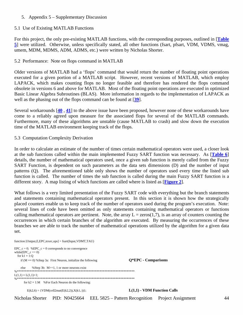
Nicholas Shorter PID: N0425664 EEL 5825 – Pattern Recognition Project Assignment 44
5. Appendix 5 – Supplementary Discussion 5.1 Use of Existing MATLAB Functions For this project, the only pre-existing MATLAB functions, with the corresponding purposes, outlined in [Table 5] were utilized. Otherwise, unless specifically stated, all other functions (fsart, pfsart, VDM, VDMS, vmag, umem, MDM, MDMS, ADM, ADMS, etc.) were written by Nicholas Shorter. 5.2 Performance: Note on flops command in MATLAB Older versions of MATLAB had a ‘flops’ command that would return the number of floating point operations executed for a given portion of a MATLAB script. However, recent versions of MATLAB, which employ LAPACK, which makes counting flops no longer feasible and therefore has rendered the flops command obsolete in versions 6 and above for MATLAB. Most of the floating point operations are executed in optimized Basic Linear Algebra Subroutines (BLAS). More information in regards to the implementation of LAPACK as well as the phasing out of the flops command can be found at [39]. Several workarounds [40 , 41] to the above issue have been proposed, however none of these workarounds have come to a reliably agreed upon measure for the associated flops for several of the MATLAB commands. Furthermore, many of these algorithms are unstable (cause MATLAB to crash) and slow down the execution time of the MATLAB environment keeping track of the flops. 5.3 Computation Complexity Derivation In order to calculate an estimate of the number of times certain mathematical operators were used, a closer look at the sub functions called within the main implemented Fuzzy SART function was necessary. As [Table 6] details, the number of mathematical operators used, once a given sub function is merely called from the Fuzzy SART Function, is dependent on such parameters as the data sets dimensions (D) and the number of input patterns (Q). The aforementioned table only shows the number of operators used every time the listed sub function is called. The number of times the sub function is called during the main Fuzzy SART function is a different story. A map listing of which functions are called where is listed as [Figure 2]. What follows is a very limited presentation of the Fuzzy SART code with everything but the branch statements and statements containing mathematical operators present. In this section it is shown how the strategically placed counters enable us to keep track of the number of operators used during the program’s execution. Note: several lines of code have been omitted as only statements containing mathematical operators or functions calling mathematical operators are pertinent. Note, the array L = zeros(1,7), is an array of counters counting the occurrences in which certain branches of the algorithm are executed. By measuring the occurrences of these branches we are able to track the number of mathematical operations utilized by the algorithm for a given data set. function [Output,E,EPC,texec,ops] = fsart(Input,VDMT,TAU) EPC_c = 0; %EPC_c = 0 corresponds to no convergence while(EPC_c == 0) for k1 = 1:Q if (M == 0) %Step 3a: First Neuron, initialize the following Q*EPC - Comparisons else %Step 3b: M>=1, 1 or more neurons exist %************************************************************************** L(1,1) = L(1,1)+1; %************************************************************************** for k2 = 1:M %For Each Neuron do the following: E(k2,6) = {VDM(cell2mat(E(k2,2)),X(k1,:))}; L(1,1) - VDM Function Calls
Nicholas Shorter PID: N0425664 EEL 5825 – Pattern Recognition Project Assignment 45
E(k2,5) = {umem(X(k1,:),cell2mat(E(k2,2)),cell2mat(E(:,2)))}; L(1,1) - umem Function Calls end [V_star,I] = max(cell2mat(E(:,6))); L(1,1)*(M-1) - Comparisons if V_star<VDMT L(1,1) - Comparisons %************************************************************************** L(1,2) = L(1,2)+1; %************************************************************************** %Vigilance Criterion Failed M = M+1; %New neuron identifier L(1,2) - Additions/Subtractions else %************************************************************************** L(1,3) = L(1,3)+1; %************************************************************************** ALPHA_star = (cell2mat(E(I,6)))^((cell2mat(E(I,1)))/TAU); L(1,3) - Powers and Divisions VDMS_star = VDMS(ALPHA_star, MDMT, ADMT, cell2mat(E(I,1)),cell2mat(E(I,5))); L(1,3) - VDMS Function Calls for k3 = 1:M ITSj = VDM((cell2mat(E(I,2))),(cell2mat(E(k3,2)))); L(1,3)*M - VDM Function Calls if ITSj > VDMS_star L(1,3)*M - Comparisons %************************************************************************** L(1,4) = L(1,4)+1; %************************************************************************** ALPHA = (cell2mat(E(k3,5)))^((cell2mat(E(k3,1))+cell2mat(E(I,1)))/TAU); L(1,4) - Powers, Additions, Divisions E(k3,2) = {(cell2mat(E(k3,2)))+ALPHA*(X(k1,:)-cell2mat(E(k3,2)))}; L(1,4) – Multiplications, 2*L(1,4) Additions/Subtractions E(k3,1) = {(cell2mat(E(k3,1)))+ALPHA}; L(1,4) - Additions else end %End Step 6a(i & ii) -> ITS check end %End Step 6 (for each Neuron peform ITS check) E(I,2) = {(cell2mat(E(I,2)))+ALPHA_star*(X(k1,:)-cell2mat(E(I,2)))}; L(1,3) – Multiplications, 2*L(1,3) Additions/Subtractions E(I,1) = {(cell2mat(E(I,1)))+ALPHA_star}; L(1,3) – Additions/Subtractions end %End of Step 5 (vigilance test) end %End of Step 3a/3b M == 0 or M>0 neuron check end %End of Step 3 (Present Input Pattern) EPC = EPC + 1; %Increment Number of Epochs for each pattern presentation EPC Additions/Subtractions if EPC == 1 EPC - Comparisons else %Epoch is greater than 1 for k5 = 1:M %************************************************************************** L(1,5) = L(1,5)+1; %************************************************************************** if cell2mat(E(k5,3)) == cell2mat(E(k5,1)) L(1,5) Comparisons %************************************************************************** L(1,6) = L(1,6)+1; %************************************************************************** M = M - 1; L(1,6) Additions/Subtractions for k6 = 1:M+1 if k6 ~= k5 %While eps is 0, all original indicies are L(1,6)*M+1 Comparisons else %Once the case where k6 == k5 or the index

Nicholas Shorter PID: N0425664 EEL 5825 – Pattern Recognition Project Assignment 46
end end else %************************************************************************** L(1,7) = L(1,7)+1; %**************************************************************************
if (vmag(cell2mat(E(k5,4))-cell2mat(E(k5,2)))>DELTA) L(1,7) vmag Function Calls, L(1,7) Comparisons, L(1,7) Additions/Subtractions
else end %end of convergence check if statement end %end of Oldtj==tj if statement end %end of for statement end %end of EPC ==1 if statement end %End of Epoch Convergence Loop From the above shortened, code presentation, the amounts of operators/function calls that were used are detailed in the following [Table 7]. Referring to [Table 6], one can see the computations utilized for function calls have also already been enumerated. Utilizing both of these sources of information yields the total number of operators utilized throughout the execution of the implemented Fuzzy SART function [Table 8].
Nicholas Shorter PID: N0425664 EEL 5825 – Pattern Recognition Project Assignment 47
6. Appendix 6 – Data Set Testing Results The data set results appendix section is composed of the following sections:
6.1 First Group of Data Set Results – g2c 6.1.1 g2c05 Data Set Results 6.1.2 g2c15 Data Set Results 6.1.3 g2c25 Data Set Results 6.1.4 g2c40 Data Set Results 6.2 Second Group of Data Set Results – g4c 6.2.1 g4c05 Data Set Results 6.2.2 g4c15 Data Set Results 6.2.3 g4c25 Data Set Results 6.2.4 g4c40 Data Set Results 6.3 irsdrg Data Set Results 6.4 New Abalon 500 Data Set Results 6.5 Nicholas Generated Data (1st generated set) 6.6 Nicholas Generated Data (2nd generated set) 6.7 pageblocks Data Set 6.8 Third Group of Data Set Results – g6c 6.8.1 g6c05 Data Set Results 6.8.2 g6c15 Data Set Results 6.8.3 g6c25 Data Set Results 6.8.4 g6c40 Data Set Results
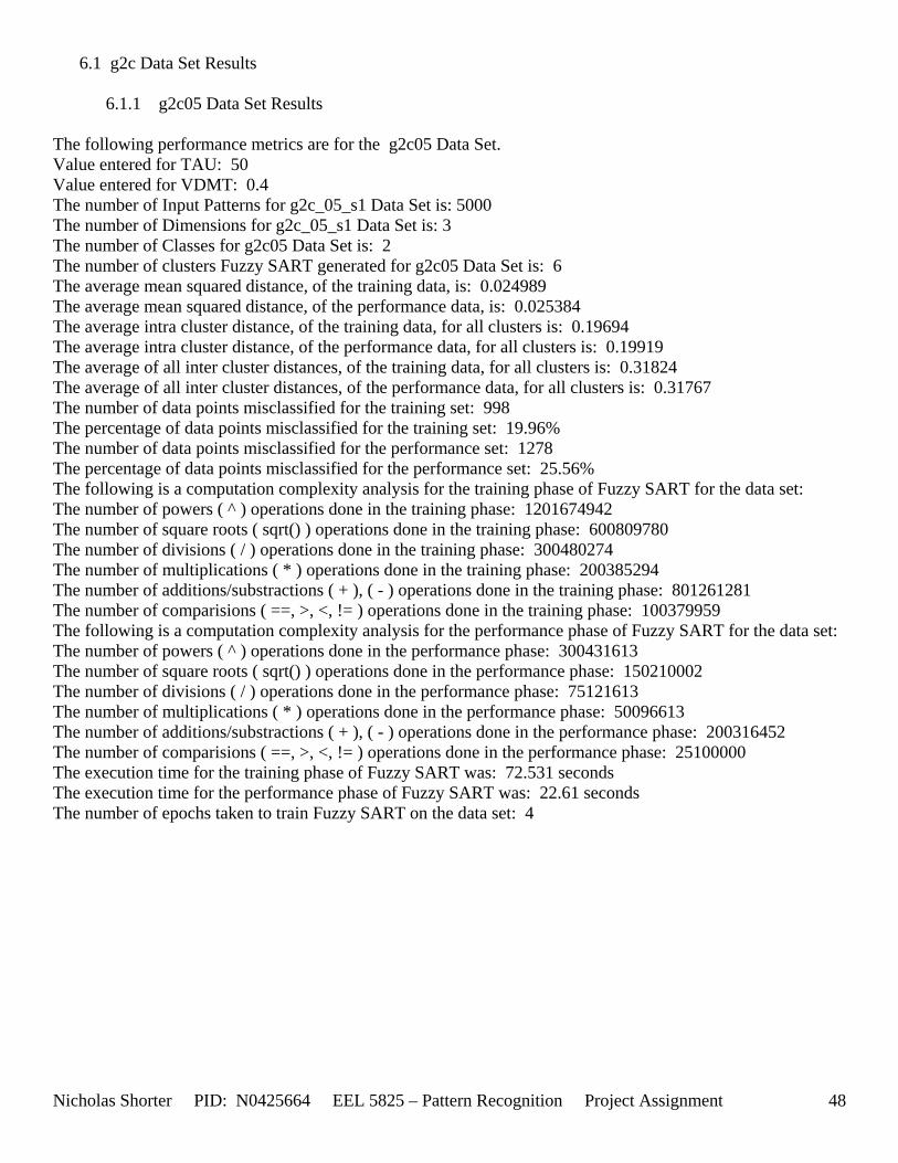
Nicholas Shorter PID: N0425664 EEL 5825 – Pattern Recognition Project Assignment 48
6.1 g2c Data Set Results
6.1.1 g2c05 Data Set Results The following performance metrics are for the g2c05 Data Set. Value entered for TAU: 50 Value entered for VDMT: 0.4 The number of Input Patterns for g2c_05_s1 Data Set is: 5000 The number of Dimensions for g2c_05_s1 Data Set is: 3 The number of Classes for g2c05 Data Set is: 2 The number of clusters Fuzzy SART generated for g2c05 Data Set is: 6 The average mean squared distance, of the training data, is: 0.024989 The average mean squared distance, of the performance data, is: 0.025384 The average intra cluster distance, of the training data, for all clusters is: 0.19694 The average intra cluster distance, of the performance data, for all clusters is: 0.19919 The average of all inter cluster distances, of the training data, for all clusters is: 0.31824 The average of all inter cluster distances, of the performance data, for all clusters is: 0.31767 The number of data points misclassified for the training set: 998 The percentage of data points misclassified for the training set: 19.96% The number of data points misclassified for the performance set: 1278 The percentage of data points misclassified for the performance set: 25.56% The following is a computation complexity analysis for the training phase of Fuzzy SART for the data set: The number of powers ( ^ ) operations done in the training phase: 1201674942 The number of square roots ( sqrt() ) operations done in the training phase: 600809780 The number of divisions ( / ) operations done in the training phase: 300480274 The number of multiplications ( * ) operations done in the training phase: 200385294 The number of additions/substractions ( + ), ( - ) operations done in the training phase: 801261281 The number of comparisions ( ==, >, <, != ) operations done in the training phase: 100379959 The following is a computation complexity analysis for the performance phase of Fuzzy SART for the data set: The number of powers ( ^ ) operations done in the performance phase: 300431613 The number of square roots ( sqrt() ) operations done in the performance phase: 150210002 The number of divisions ( / ) operations done in the performance phase: 75121613 The number of multiplications ( * ) operations done in the performance phase: 50096613 The number of additions/substractions ( + ), ( - ) operations done in the performance phase: 200316452 The number of comparisions ( ==, >, <, != ) operations done in the performance phase: 25100000 The execution time for the training phase of Fuzzy SART was: 72.531 seconds The execution time for the performance phase of Fuzzy SART was: 22.61 seconds The number of epochs taken to train Fuzzy SART on the data set: 4
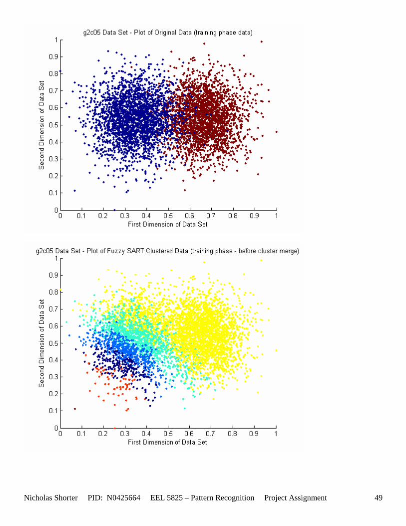
Nicholas Shorter PID: N0425664 EEL 5825 – Pattern Recognition Project Assignment 49
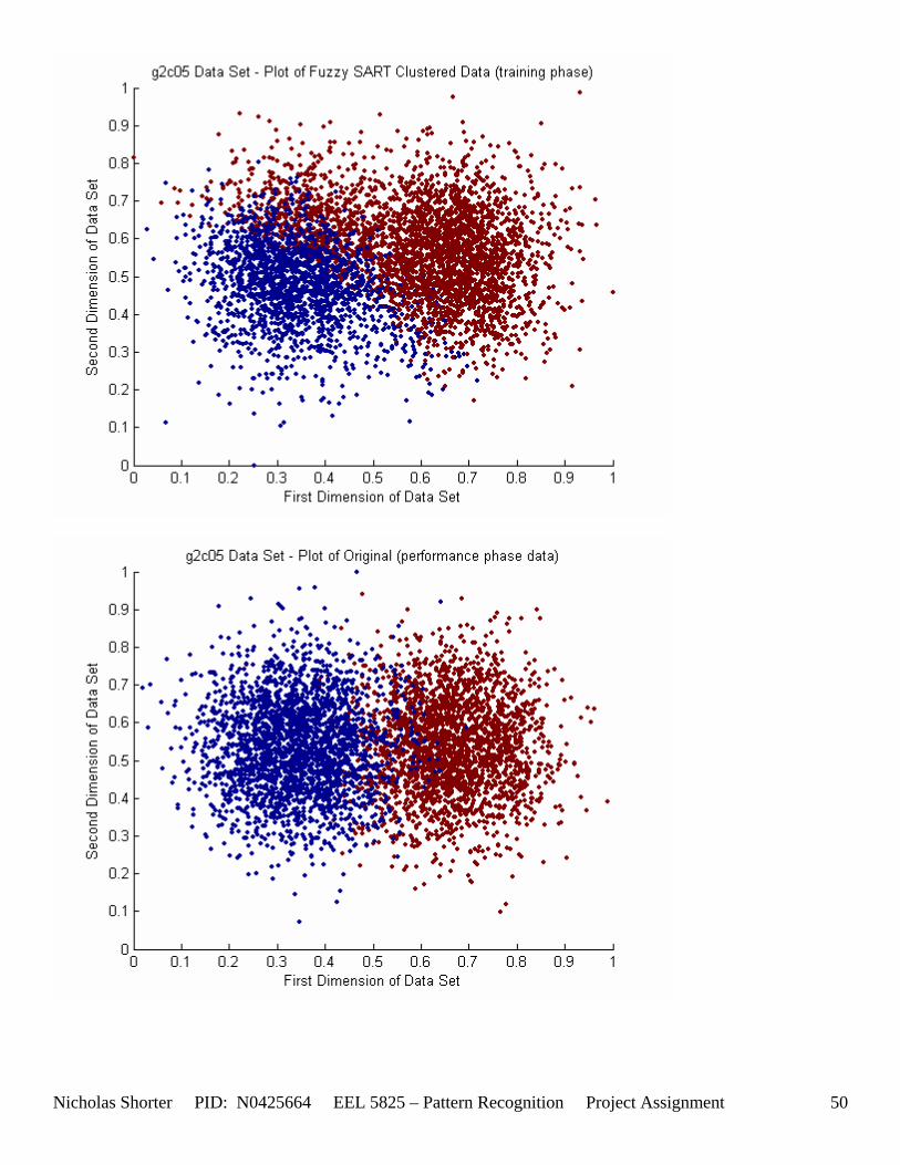
Nicholas Shorter PID: N0425664 EEL 5825 – Pattern Recognition Project Assignment 50
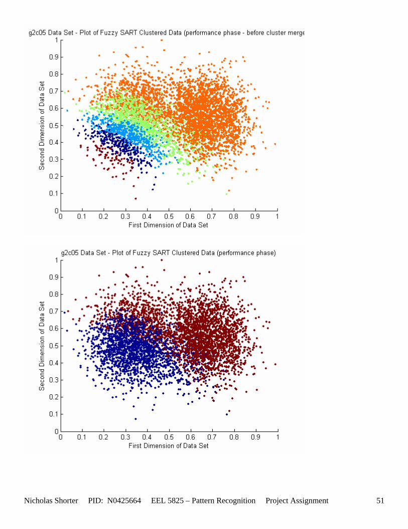
Nicholas Shorter PID: N0425664 EEL 5825 – Pattern Recognition Project Assignment 51
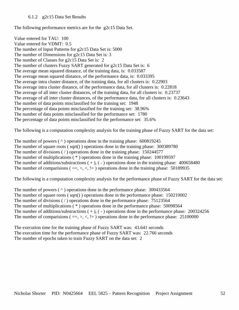
Nicholas Shorter PID: N0425664 EEL 5825 – Pattern Recognition Project Assignment 52
6.1.2 g2c15 Data Set Results The following performance metrics are for the g2c15 Data Set. Value entered for TAU: 100 Value entered for VDMT: 0.5 The number of Input Patterns for g2c15 Data Set is: 5000 The number of Dimensions for g2c15 Data Set is: 3 The number of Classes for g2c15 Data Set is: 2 The number of clusters Fuzzy SART generated for g2c15 Data Set is: 6 The average mean squared distance, of the training data, is: 0.033587 The average mean squared distance, of the performance data, is: 0.033395 The average intra cluster distance, of the training data, for all clusters is: 0.22903 The average intra cluster distance, of the performance data, for all clusters is: 0.22818 The average of all inter cluster distances, of the training data, for all clusters is: 0.23737 The average of all inter cluster distances, of the performance data, for all clusters is: 0.23643 The number of data points misclassified for the training set: 1948 The percentage of data points misclassified for the training set: 38.96% The number of data points misclassified for the performance set: 1780 The percentage of data points misclassified for the performance set: 35.6% The following is a computation complexity analysis for the training phase of Fuzzy SART for the data set: The number of powers ( ^ ) operations done in the training phase: 600819245 The number of square roots ( sqrt() ) operations done in the training phase: 300389780 The number of divisions ( / ) operations done in the training phase: 150244577 The number of multiplications ( * ) operations done in the training phase: 100199597 The number of additions/substractions ( + ), ( - ) operations done in the training phase: 400658480 The number of comparisions ( ==, >, <, != ) operations done in the training phase: 50189935 The following is a computation complexity analysis for the performance phase of Fuzzy SART for the data set: The number of powers ( ^ ) operations done in the performance phase: 300433564 The number of square roots ( sqrt() ) operations done in the performance phase: 150210002 The number of divisions ( / ) operations done in the performance phase: 75123564 The number of multiplications ( * ) operations done in the performance phase: 50098564 The number of additions/substractions ( + ), ( - ) operations done in the performance phase: 200324256 The number of comparisions ( ==, >, <, != ) operations done in the performance phase: 25100000 The execution time for the training phase of Fuzzy SART was: 43.641 seconds The execution time for the performance phase of Fuzzy SART was: 22.766 seconds The number of epochs taken to train Fuzzy SART on the data set: 2
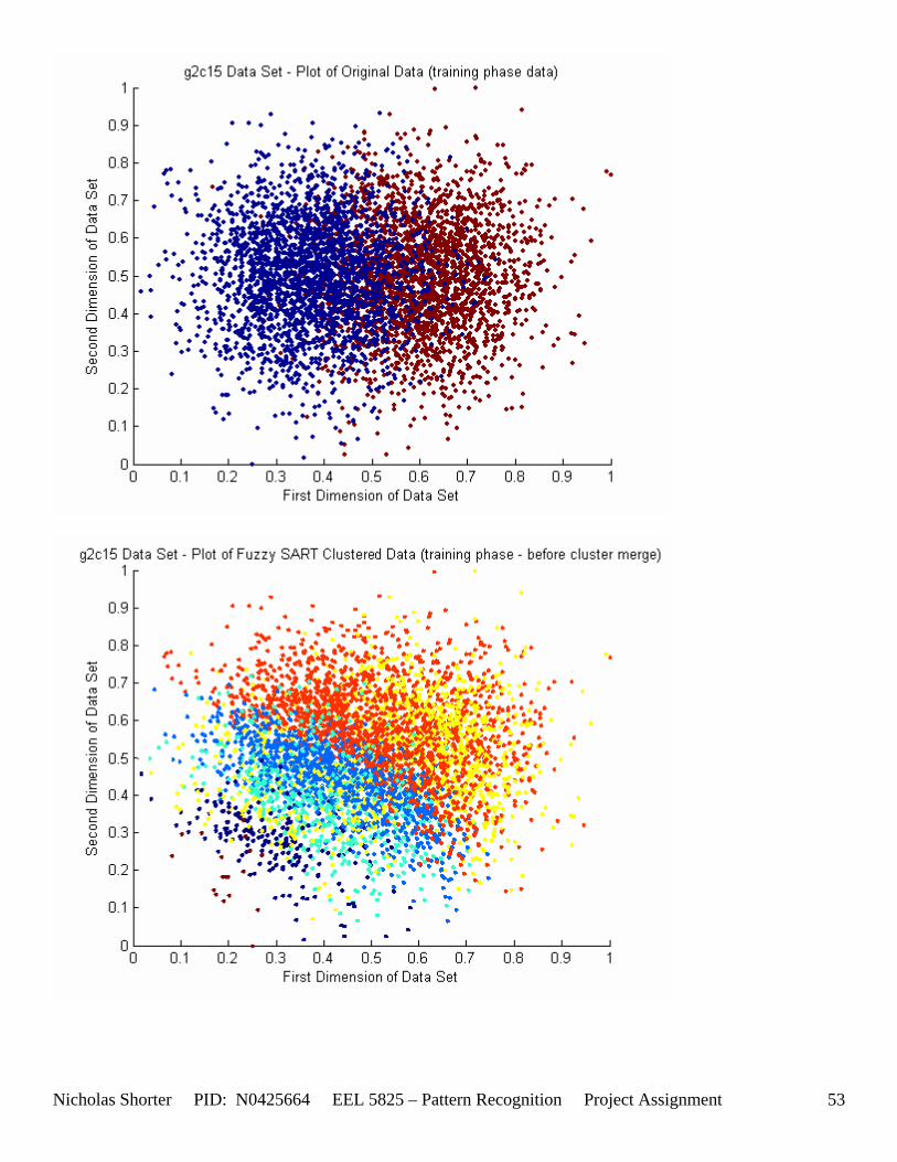
Nicholas Shorter PID: N0425664 EEL 5825 – Pattern Recognition Project Assignment 53
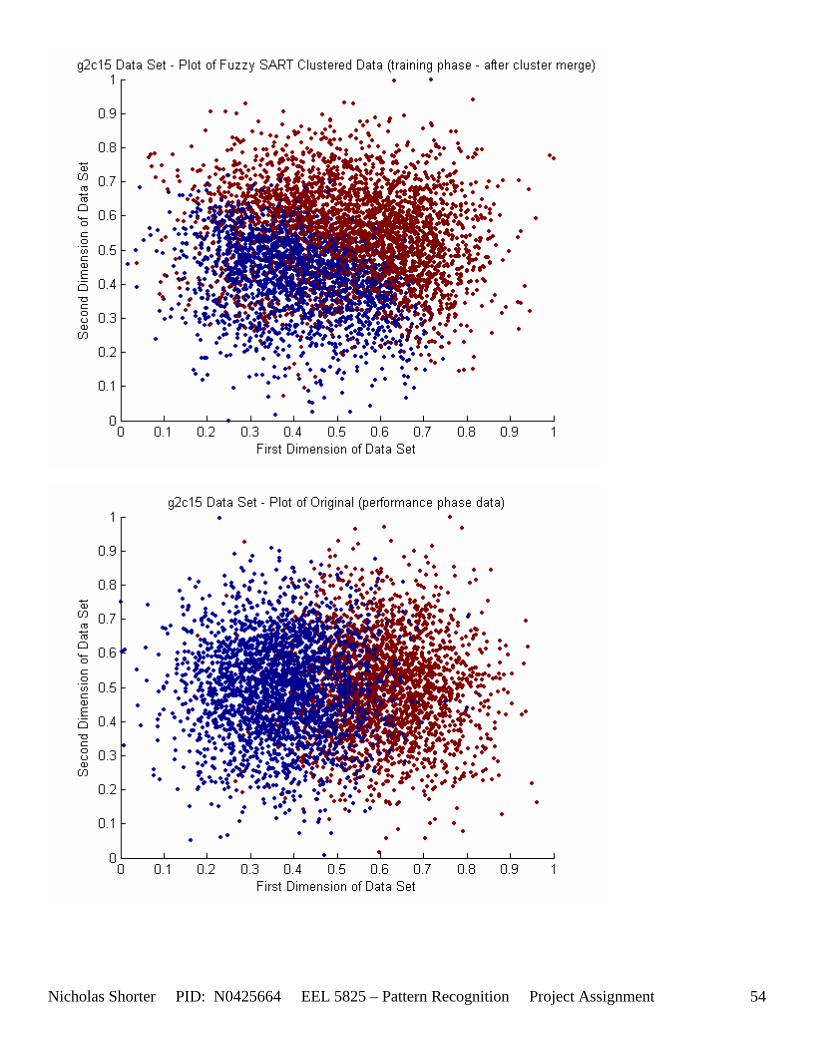
Nicholas Shorter PID: N0425664 EEL 5825 – Pattern Recognition Project Assignment 54
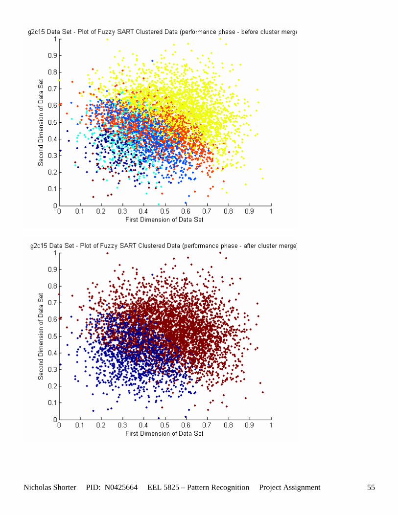
Nicholas Shorter PID: N0425664 EEL 5825 – Pattern Recognition Project Assignment 55
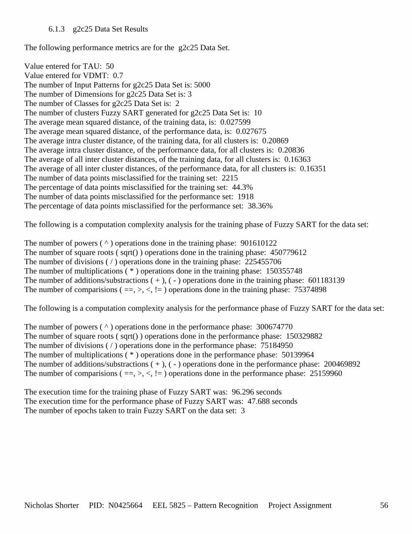
Nicholas Shorter PID: N0425664 EEL 5825 – Pattern Recognition Project Assignment 56
6.1.3 g2c25 Data Set Results
The following performance metrics are for the g2c25 Data Set. Value entered for TAU: 50 Value entered for VDMT: 0.7 The number of Input Patterns for g2c25 Data Set is: 5000 The number of Dimensions for g2c25 Data Set is: 3 The number of Classes for g2c25 Data Set is: 2 The number of clusters Fuzzy SART generated for g2c25 Data Set is: 10 The average mean squared distance, of the training data, is: 0.027599 The average mean squared distance, of the performance data, is: 0.027675 The average intra cluster distance, of the training data, for all clusters is: 0.20869 The average intra cluster distance, of the performance data, for all clusters is: 0.20836 The average of all inter cluster distances, of the training data, for all clusters is: 0.16363 The average of all inter cluster distances, of the performance data, for all clusters is: 0.16351 The number of data points misclassified for the training set: 2215 The percentage of data points misclassified for the training set: 44.3% The number of data points misclassified for the performance set: 1918 The percentage of data points misclassified for the performance set: 38.36% The following is a computation complexity analysis for the training phase of Fuzzy SART for the data set: The number of powers ( ^ ) operations done in the training phase: 901610122 The number of square roots ( sqrt() ) operations done in the training phase: 450779612 The number of divisions ( / ) operations done in the training phase: 225455706 The number of multiplications ( * ) operations done in the training phase: 150355748 The number of additions/substractions ( + ), ( - ) operations done in the training phase: 601183139 The number of comparisions ( ==, >, <, != ) operations done in the training phase: 75374898 The following is a computation complexity analysis for the performance phase of Fuzzy SART for the data set: The number of powers ( ^ ) operations done in the performance phase: 300674770 The number of square roots ( sqrt() ) operations done in the performance phase: 150329882 The number of divisions ( / ) operations done in the performance phase: 75184950 The number of multiplications ( * ) operations done in the performance phase: 50139964 The number of additions/substractions ( + ), ( - ) operations done in the performance phase: 200469892 The number of comparisions ( ==, >, <, != ) operations done in the performance phase: 25159960 The execution time for the training phase of Fuzzy SART was: 96.296 seconds The execution time for the performance phase of Fuzzy SART was: 47.688 seconds The number of epochs taken to train Fuzzy SART on the data set: 3
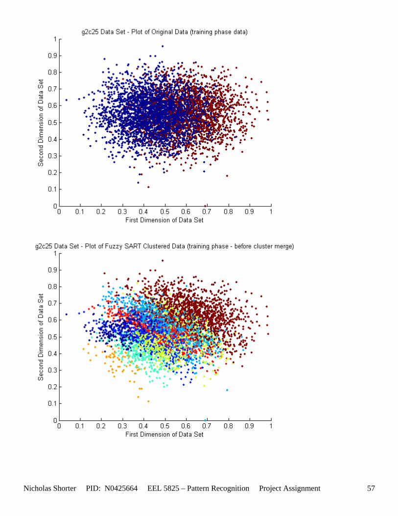
Nicholas Shorter PID: N0425664 EEL 5825 – Pattern Recognition Project Assignment 57
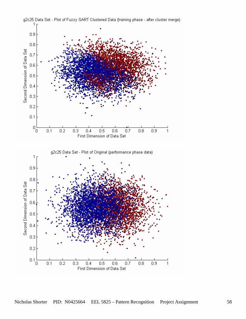
Nicholas Shorter PID: N0425664 EEL 5825 – Pattern Recognition Project Assignment 58
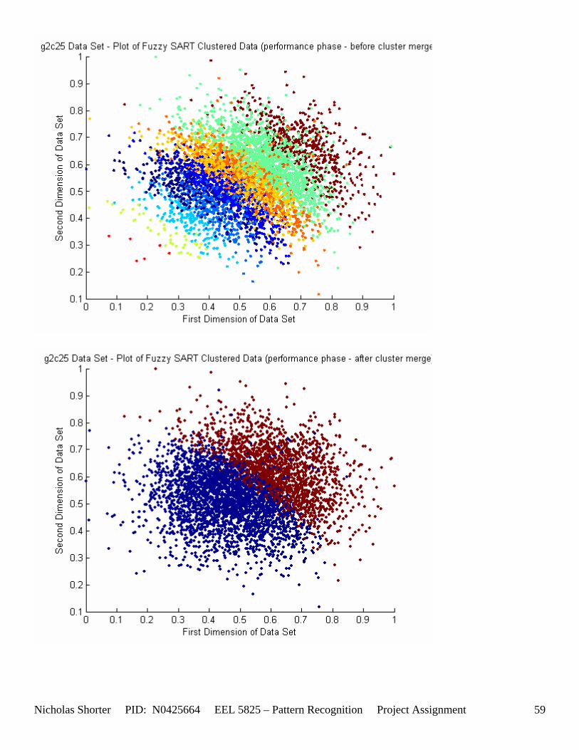
Nicholas Shorter PID: N0425664 EEL 5825 – Pattern Recognition Project Assignment 59
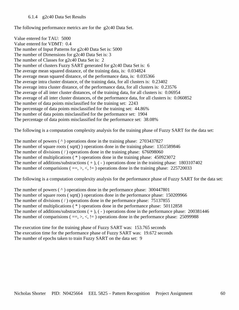
Nicholas Shorter PID: N0425664 EEL 5825 – Pattern Recognition Project Assignment 60
6.1.4 g2c40 Data Set Results The following performance metrics are for the g2c40 Data Set. Value entered for TAU: 5000 Value entered for VDMT: 0.4 The number of Input Patterns for g2c40 Data Set is: 5000 The number of Dimensions for g2c40 Data Set is: 3 The number of Classes for g2c40 Data Set is: 2 The number of clusters Fuzzy SART generated for g2c40 Data Set is: 6 The average mean squared distance, of the training data, is: 0.034824 The average mean squared distance, of the performance data, is: 0.035366 The average intra cluster distance, of the training data, for all clusters is: 0.23402 The average intra cluster distance, of the performance data, for all clusters is: 0.23576 The average of all inter cluster distances, of the training data, for all clusters is: 0.06954 The average of all inter cluster distances, of the performance data, for all clusters is: 0.060852 The number of data points misclassified for the training set: 2243 The percentage of data points misclassified for the training set: 44.86% The number of data points misclassified for the performance set: 1904 The percentage of data points misclassified for the performance set: 38.08% The following is a computation complexity analysis for the training phase of Fuzzy SART for the data set: The number of powers ( ^ ) operations done in the training phase: 2703437827 The number of square roots ( sqrt() ) operations done in the training phase: 1351589846 The number of divisions ( / ) operations done in the training phase: 676098060 The number of multiplications ( * ) operations done in the training phase: 450923072 The number of additions/substractions ( + ), ( - ) operations done in the training phase: 1803107402 The number of comparisions ( ==, >, <, != ) operations done in the training phase: 225720033 The following is a computation complexity analysis for the performance phase of Fuzzy SART for the data set: The number of powers ( ^ ) operations done in the performance phase: 300447801 The number of square roots ( sqrt() ) operations done in the performance phase: 150209966 The number of divisions ( / ) operations done in the performance phase: 75137855 The number of multiplications ( * ) operations done in the performance phase: 50112858 The number of additions/substractions ( + ), ( - ) operations done in the performance phase: 200381446 The number of comparisions ( ==, >, <, != ) operations done in the performance phase: 25099988 The execution time for the training phase of Fuzzy SART was: 153.765 seconds The execution time for the performance phase of Fuzzy SART was: 19.672 seconds The number of epochs taken to train Fuzzy SART on the data set: 9
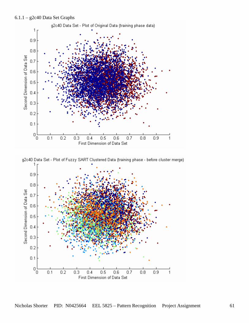
6.1.1 – g2c40 Data Set Graphs
Nicholas Shorter PID: N0425664 EEL 5825 – Pattern Recognition Project Assignment 61
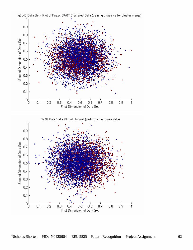
Nicholas Shorter PID: N0425664 EEL 5825 – Pattern Recognition Project Assignment 62
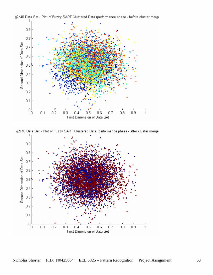
Nicholas Shorter PID: N0425664 EEL 5825 – Pattern Recognition Project Assignment 63
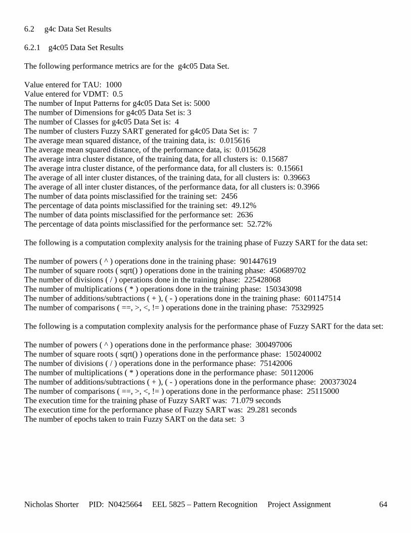
Nicholas Shorter PID: N0425664 EEL 5825 – Pattern Recognition Project Assignment 64
6.2 g4c Data Set Results 6.2.1 g4c05 Data Set Results The following performance metrics are for the g4c05 Data Set. Value entered for TAU: 1000 Value entered for VDMT: 0.5 The number of Input Patterns for g4c05 Data Set is: 5000 The number of Dimensions for g4c05 Data Set is: 3 The number of Classes for g4c05 Data Set is: 4 The number of clusters Fuzzy SART generated for g4c05 Data Set is: 7 The average mean squared distance, of the training data, is: 0.015616 The average mean squared distance, of the performance data, is: 0.015628 The average intra cluster distance, of the training data, for all clusters is: 0.15687 The average intra cluster distance, of the performance data, for all clusters is: 0.15661 The average of all inter cluster distances, of the training data, for all clusters is: 0.39663 The average of all inter cluster distances, of the performance data, for all clusters is: 0.3966 The number of data points misclassified for the training set: 2456 The percentage of data points misclassified for the training set: 49.12% The number of data points misclassified for the performance set: 2636 The percentage of data points misclassified for the performance set: 52.72% The following is a computation complexity analysis for the training phase of Fuzzy SART for the data set: The number of powers ( ^ ) operations done in the training phase: 901447619 The number of square roots ( sqrt() ) operations done in the training phase: 450689702 The number of divisions ( / ) operations done in the training phase: 225428068 The number of multiplications ( * ) operations done in the training phase: 150343098 The number of additions/subtractions ( + ), ( - ) operations done in the training phase: 601147514 The number of comparisons ( ==, >, <, != ) operations done in the training phase: 75329925 The following is a computation complexity analysis for the performance phase of Fuzzy SART for the data set: The number of powers ( ^ ) operations done in the performance phase: 300497006 The number of square roots ( sqrt() ) operations done in the performance phase: 150240002 The number of divisions ( / ) operations done in the performance phase: 75142006 The number of multiplications ( * ) operations done in the performance phase: 50112006 The number of additions/subtractions ( + ), ( - ) operations done in the performance phase: 200373024 The number of comparisons ( ==, >, <, != ) operations done in the performance phase: 25115000 The execution time for the training phase of Fuzzy SART was: 71.079 seconds The execution time for the performance phase of Fuzzy SART was: 29.281 seconds The number of epochs taken to train Fuzzy SART on the data set: 3
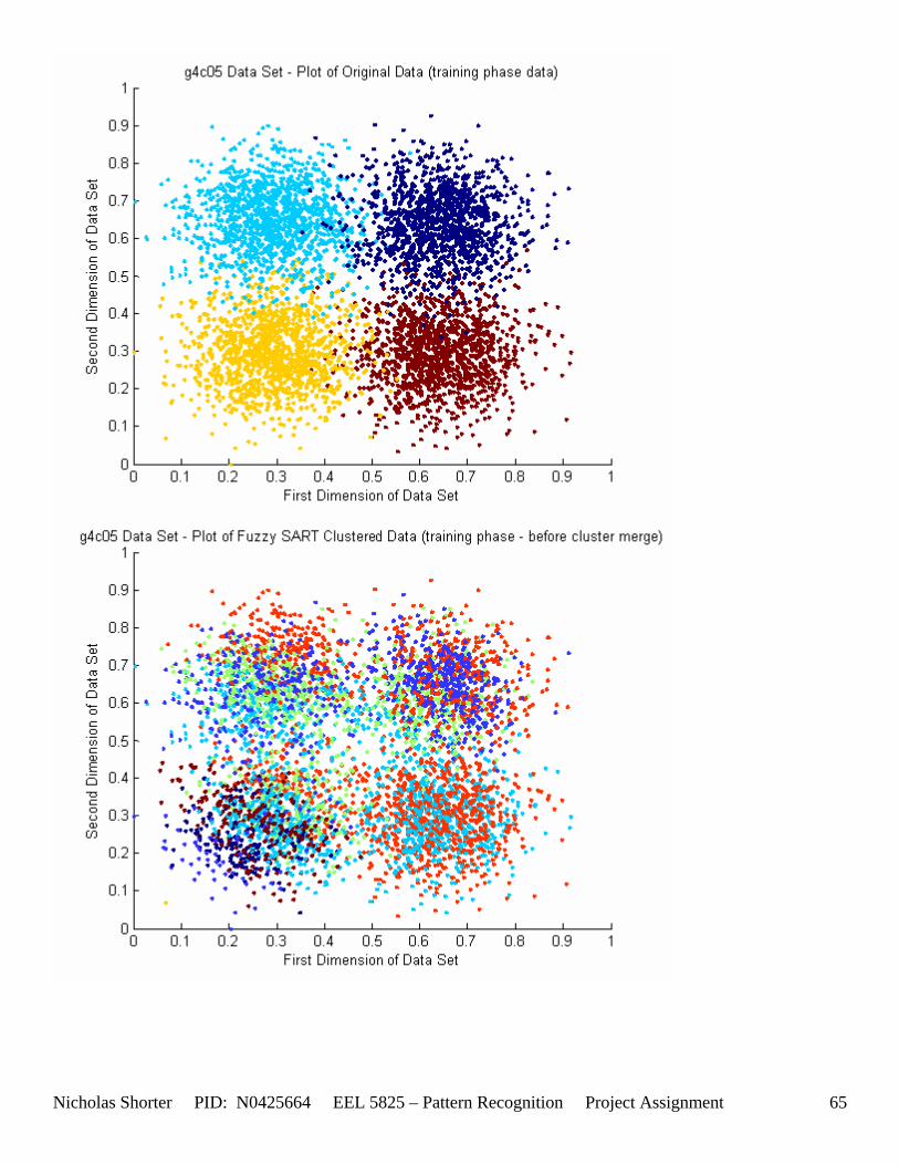
Nicholas Shorter PID: N0425664 EEL 5825 – Pattern Recognition Project Assignment 65
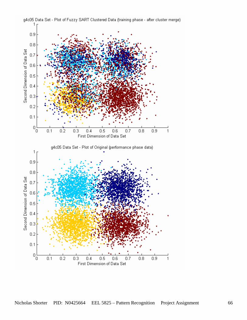
Nicholas Shorter PID: N0425664 EEL 5825 – Pattern Recognition Project Assignment 66
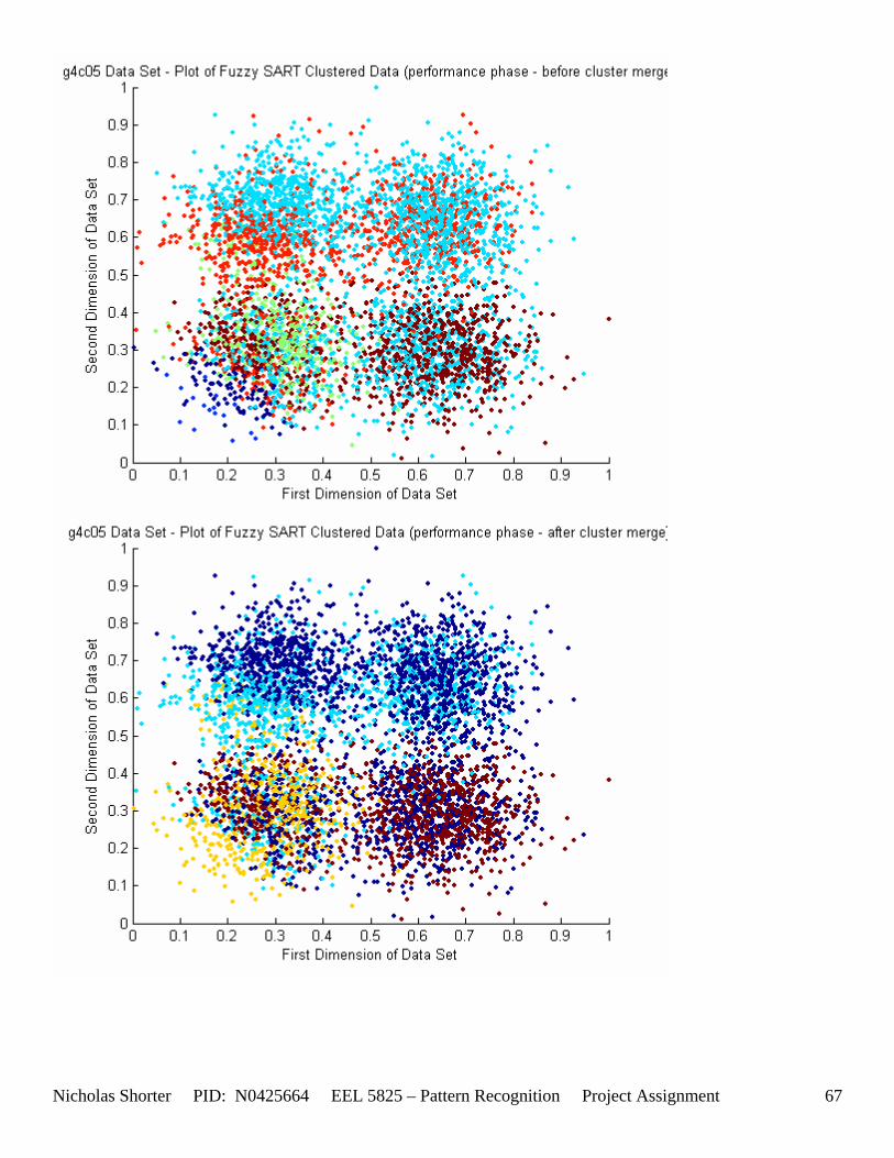
Nicholas Shorter PID: N0425664 EEL 5825 – Pattern Recognition Project Assignment 67
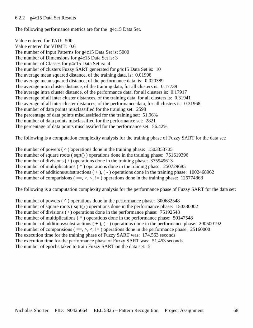
Nicholas Shorter PID: N0425664 EEL 5825 – Pattern Recognition Project Assignment 68
6.2.2 g4c15 Data Set Results The following performance metrics are for the g4c15 Data Set. Value entered for TAU: 500 Value entered for VDMT: 0.6 The number of Input Patterns for g4c15 Data Set is: 5000 The number of Dimensions for g4c15 Data Set is: 3 The number of Classes for g4c15 Data Set is: 4 The number of clusters Fuzzy SART generated for g4c15 Data Set is: 10 The average mean squared distance, of the training data, is: 0.01998 The average mean squared distance, of the performance data, is: 0.020389 The average intra cluster distance, of the training data, for all clusters is: 0.17739 The average intra cluster distance, of the performance data, for all clusters is: 0.17917 The average of all inter cluster distances, of the training data, for all clusters is: 0.31941 The average of all inter cluster distances, of the performance data, for all clusters is: 0.31968 The number of data points misclassified for the training set: 2598 The percentage of data points misclassified for the training set: 51.96% The number of data points misclassified for the performance set: 2821 The percentage of data points misclassified for the performance set: 56.42% The following is a computation complexity analysis for the training phase of Fuzzy SART for the data set: The number of powers ( ^ ) operations done in the training phase: 1503353705 The number of square roots ( sqrt() ) operations done in the training phase: 751619396 The number of divisions ( / ) operations done in the training phase: 375949613 The number of multiplications ( * ) operations done in the training phase: 250729685 The number of additions/substractions ( + ), ( - ) operations done in the training phase: 1002468962 The number of comparisions ( ==, >, <, != ) operations done in the training phase: 125774868 The following is a computation complexity analysis for the performance phase of Fuzzy SART for the data set: The number of powers ( ^ ) operations done in the performance phase: 300682548 The number of square roots ( sqrt() ) operations done in the performance phase: 150330002 The number of divisions ( / ) operations done in the performance phase: 75192548 The number of multiplications ( * ) operations done in the performance phase: 50147548 The number of additions/substractions ( + ), ( - ) operations done in the performance phase: 200500192 The number of comparisions ( ==, >, <, != ) operations done in the performance phase: 25160000 The execution time for the training phase of Fuzzy SART was: 174.563 seconds The execution time for the performance phase of Fuzzy SART was: 51.453 seconds The number of epochs taken to train Fuzzy SART on the data set: 5
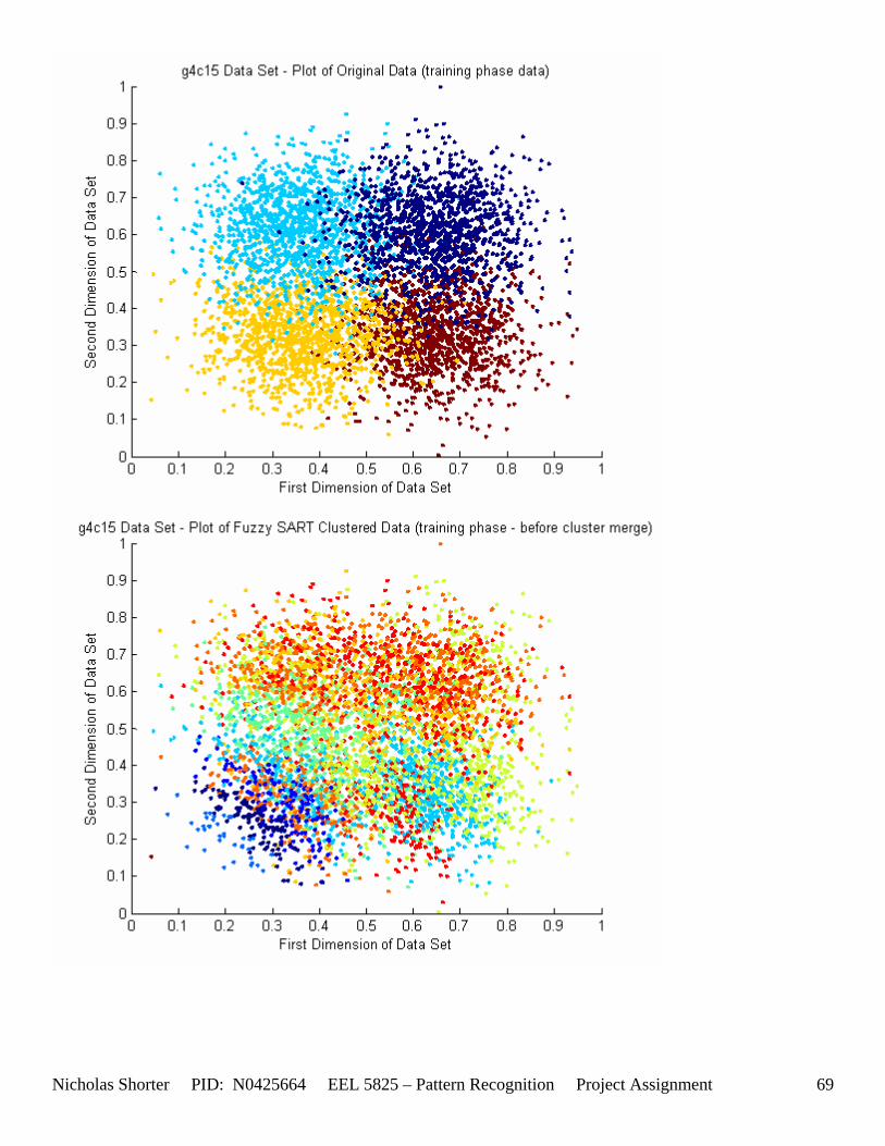
Nicholas Shorter PID: N0425664 EEL 5825 – Pattern Recognition Project Assignment 69
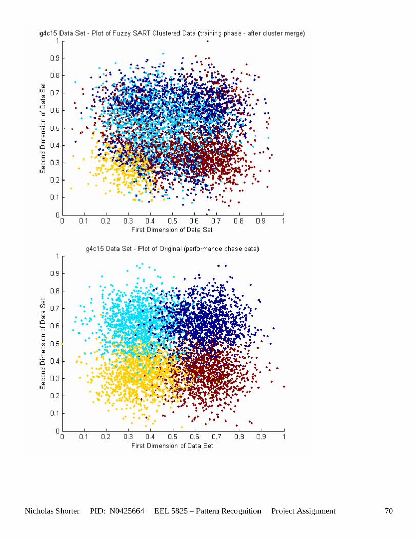
Nicholas Shorter PID: N0425664 EEL 5825 – Pattern Recognition Project Assignment 70
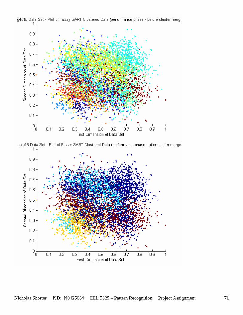
Nicholas Shorter PID: N0425664 EEL 5825 – Pattern Recognition Project Assignment 71

Nicholas Shorter PID: N0425664 EEL 5825 – Pattern Recognition Project Assignment 72
6.2.3 g4c25 Data Set Results The following performance metrics are for the g4c25 Data Set. Value entered for TAU: 500 Value entered for VDMT: 0.6 The number of Input Patterns for g4c25 Data Set is: 5000 The number of Dimensions for g4c25 Data Set is: 3 The number of Classes for g4c25 Data Set is: 4 The number of clusters Fuzzy SART generated for g4c25 Data Set is: 10 The average mean squared distance, of the training data, is: 0.02272 The average mean squared distance, of the performance data, is: 0.021932 The average intra cluster distance, of the training data, for all clusters is: 0.18875 The average intra cluster distance, of the performance data, for all clusters is: 0.18559 The average of all inter cluster distances, of the training data, for all clusters is: 0.26359 The average of all inter cluster distances, of the performance data, for all clusters is: 0.26626 The number of data points misclassified for the training set: 3233 The percentage of data points misclassified for the training set: 64.66% The number of data points misclassified for the performance set: 3044 The percentage of data points misclassified for the performance set: 60.88% The following is a computation complexity analysis for the training phase of Fuzzy SART for the data set: The number of powers ( ^ ) operations done in the training phase: 1502745812 The number of square roots ( sqrt() ) operations done in the training phase: 751319612 The number of divisions ( / ) operations done in the training phase: 375791396 The number of multiplications ( * ) operations done in the training phase: 250621438 The number of additions/substractions ( + ), ( - ) operations done in the training phase: 1002085913 The number of comparisions ( ==, >, <, != ) operations done in the training phase: 125624924 The following is a computation complexity analysis for the performance phase of Fuzzy SART for the data set: The number of powers ( ^ ) operations done in the performance phase: 300682342 The number of square roots ( sqrt() ) operations done in the performance phase: 150329882 The number of divisions ( / ) operations done in the performance phase: 75192522 The number of multiplications ( * ) operations done in the performance phase: 50147536 The number of additions/substractions ( + ), ( - ) operations done in the performance phase: 200500180 The number of comparisions ( ==, >, <, != ) operations done in the performance phase: 25159960 The execution time for the training phase of Fuzzy SART was: 122.312 seconds The execution time for the performance phase of Fuzzy SART was: 41.594 seconds The number of epochs taken to train Fuzzy SART on the data set: 5
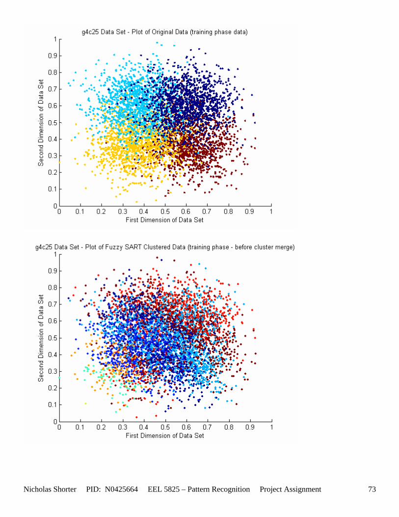
Nicholas Shorter PID: N0425664 EEL 5825 – Pattern Recognition Project Assignment 73
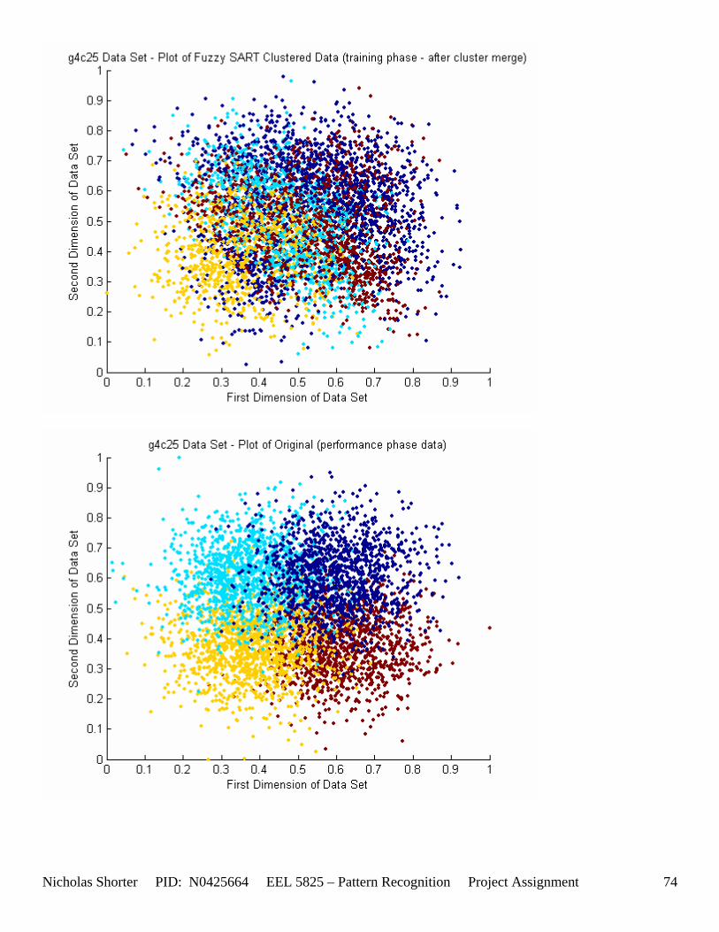
Nicholas Shorter PID: N0425664 EEL 5825 – Pattern Recognition Project Assignment 74
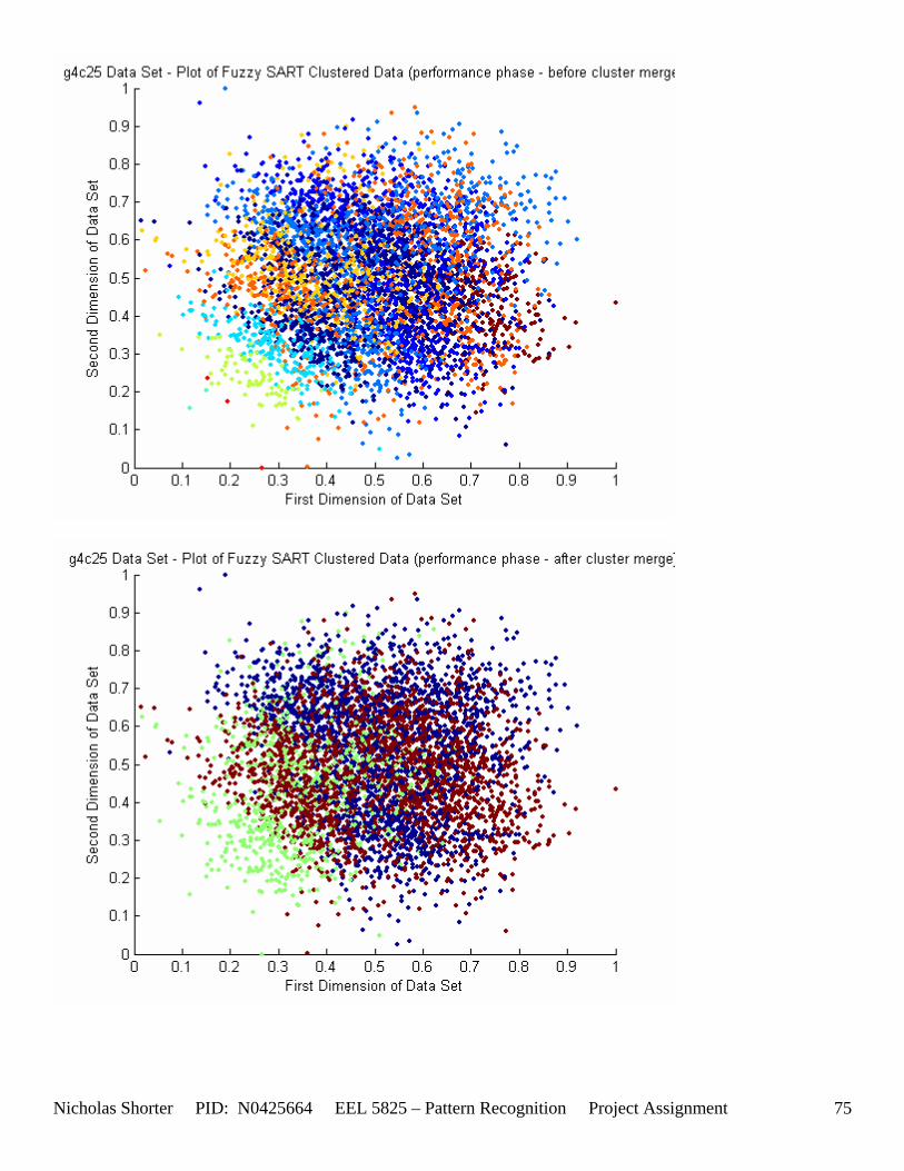
Nicholas Shorter PID: N0425664 EEL 5825 – Pattern Recognition Project Assignment 75
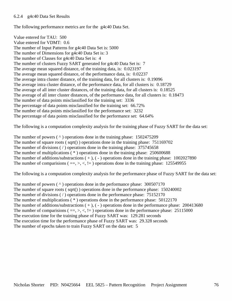
Nicholas Shorter PID: N0425664 EEL 5825 – Pattern Recognition Project Assignment 76
6.2.4 g4c40 Data Set Results The following performance metrics are for the g4c40 Data Set. Value entered for TAU: 500 Value entered for VDMT: 0.6 The number of Input Patterns for g4c40 Data Set is: 5000 The number of Dimensions for g4c40 Data Set is: 3 The number of Classes for g4c40 Data Set is: 4 The number of clusters Fuzzy SART generated for g4c40 Data Set is: 7 The average mean squared distance, of the training data, is: 0.023197 The average mean squared distance, of the performance data, is: 0.02237 The average intra cluster distance, of the training data, for all clusters is: 0.19096 The average intra cluster distance, of the performance data, for all clusters is: 0.18729 The average of all inter cluster distances, of the training data, for all clusters is: 0.18525 The average of all inter cluster distances, of the performance data, for all clusters is: 0.18473 The number of data points misclassified for the training set: 3336 The percentage of data points misclassified for the training set: 66.72% The number of data points misclassified for the performance set: 3232 The percentage of data points misclassified for the performance set: 64.64% The following is a computation complexity analysis for the training phase of Fuzzy SART for the data set: The number of powers ( ^ ) operations done in the training phase: 1502475209 The number of square roots ( sqrt() ) operations done in the training phase: 751169702 The number of divisions ( / ) operations done in the training phase: 375745658 The number of multiplications ( * ) operations done in the training phase: 250600688 The number of additions/substractions ( + ), ( - ) operations done in the training phase: 1002027890 The number of comparisions ( ==, >, <, != ) operations done in the training phase: 125549955 The following is a computation complexity analysis for the performance phase of Fuzzy SART for the data set: The number of powers ( ^ ) operations done in the performance phase: 300507170 The number of square roots ( sqrt() ) operations done in the performance phase: 150240002 The number of divisions ( / ) operations done in the performance phase: 75152170 The number of multiplications ( * ) operations done in the performance phase: 50122170 The number of additions/substractions ( + ), ( - ) operations done in the performance phase: 200413680 The number of comparisions ( ==, >, <, != ) operations done in the performance phase: 25115000 The execution time for the training phase of Fuzzy SART was: 129.281 seconds The execution time for the performance phase of Fuzzy SART was: 29.328 seconds The number of epochs taken to train Fuzzy SART on the data set: 5
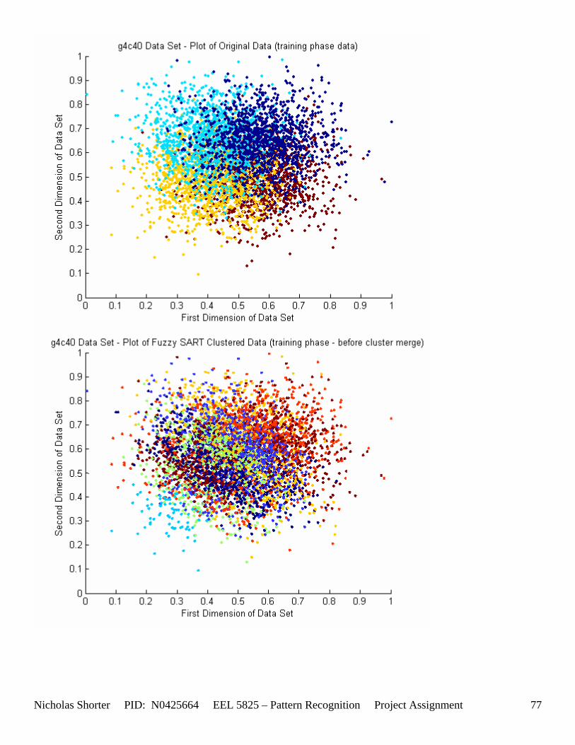
Nicholas Shorter PID: N0425664 EEL 5825 – Pattern Recognition Project Assignment 77
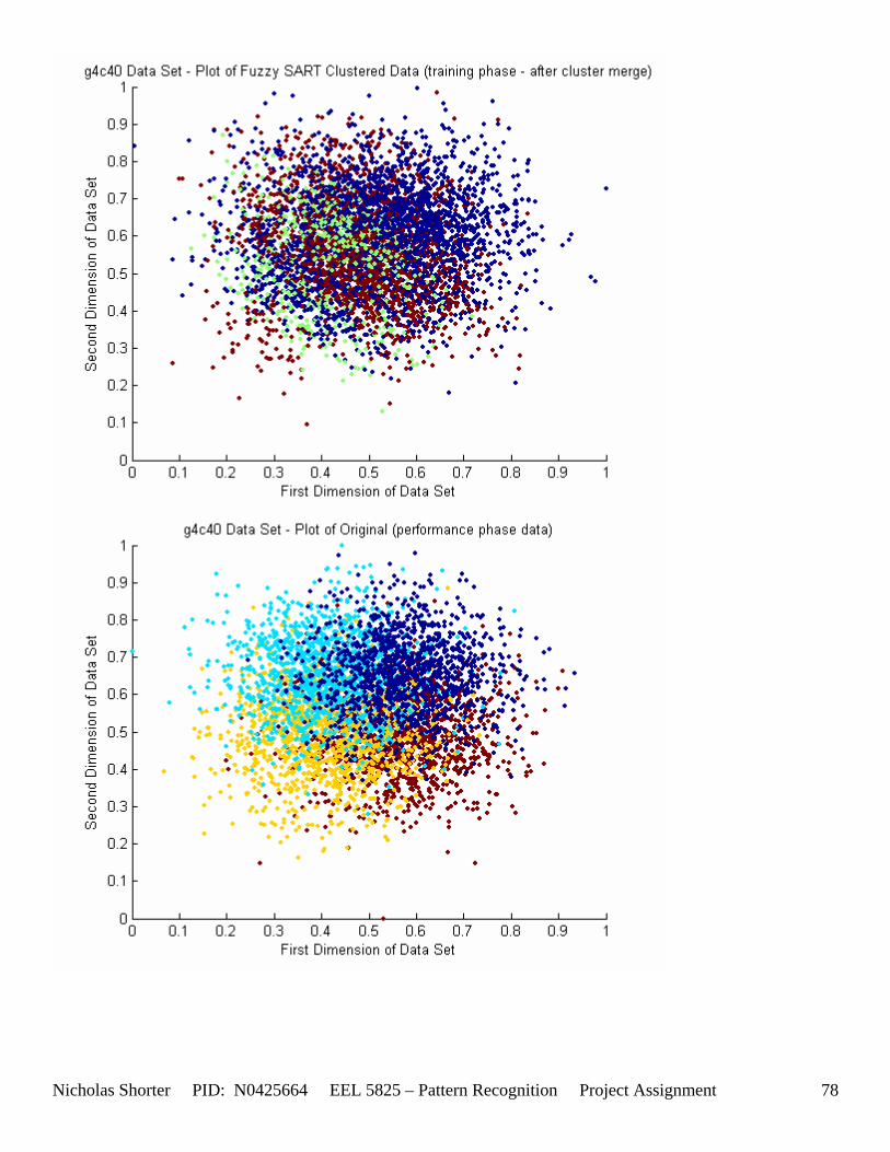
Nicholas Shorter PID: N0425664 EEL 5825 – Pattern Recognition Project Assignment 78
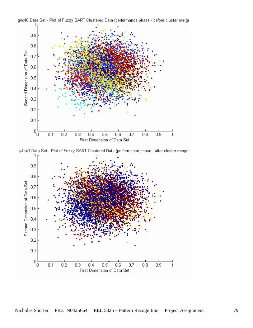
Nicholas Shorter PID: N0425664 EEL 5825 – Pattern Recognition Project Assignment 79
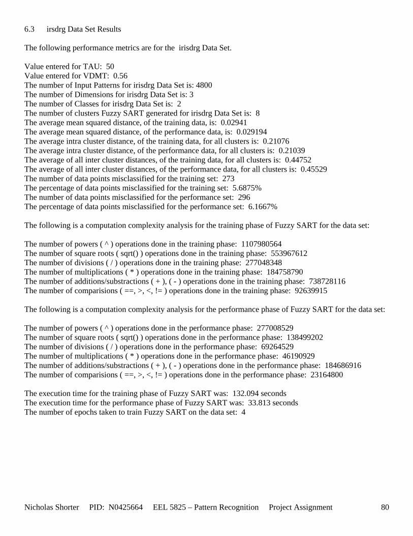
Nicholas Shorter PID: N0425664 EEL 5825 – Pattern Recognition Project Assignment 80
6.3 irsdrg Data Set Results The following performance metrics are for the irisdrg Data Set. Value entered for TAU: 50 Value entered for VDMT: 0.56 The number of Input Patterns for irisdrg Data Set is: 4800 The number of Dimensions for irisdrg Data Set is: 3 The number of Classes for irisdrg Data Set is: 2 The number of clusters Fuzzy SART generated for irisdrg Data Set is: 8 The average mean squared distance, of the training data, is: 0.02941 The average mean squared distance, of the performance data, is: 0.029194 The average intra cluster distance, of the training data, for all clusters is: 0.21076 The average intra cluster distance, of the performance data, for all clusters is: 0.21039 The average of all inter cluster distances, of the training data, for all clusters is: 0.44752 The average of all inter cluster distances, of the performance data, for all clusters is: 0.45529 The number of data points misclassified for the training set: 273 The percentage of data points misclassified for the training set: 5.6875% The number of data points misclassified for the performance set: 296 The percentage of data points misclassified for the performance set: 6.1667% The following is a computation complexity analysis for the training phase of Fuzzy SART for the data set: The number of powers ( ^ ) operations done in the training phase: 1107980564 The number of square roots ( sqrt() ) operations done in the training phase: 553967612 The number of divisions ( / ) operations done in the training phase: 277048348 The number of multiplications ( * ) operations done in the training phase: 184758790 The number of additions/substractions ( + ), ( - ) operations done in the training phase: 738728116 The number of comparisions ( ==, >, <, != ) operations done in the training phase: 92639915 The following is a computation complexity analysis for the performance phase of Fuzzy SART for the data set: The number of powers ( ^ ) operations done in the performance phase: 277008529 The number of square roots ( sqrt() ) operations done in the performance phase: 138499202 The number of divisions ( / ) operations done in the performance phase: 69264529 The number of multiplications ( * ) operations done in the performance phase: 46190929 The number of additions/substractions ( + ), ( - ) operations done in the performance phase: 184686916 The number of comparisions ( ==, >, <, != ) operations done in the performance phase: 23164800 The execution time for the training phase of Fuzzy SART was: 132.094 seconds The execution time for the performance phase of Fuzzy SART was: 33.813 seconds The number of epochs taken to train Fuzzy SART on the data set: 4
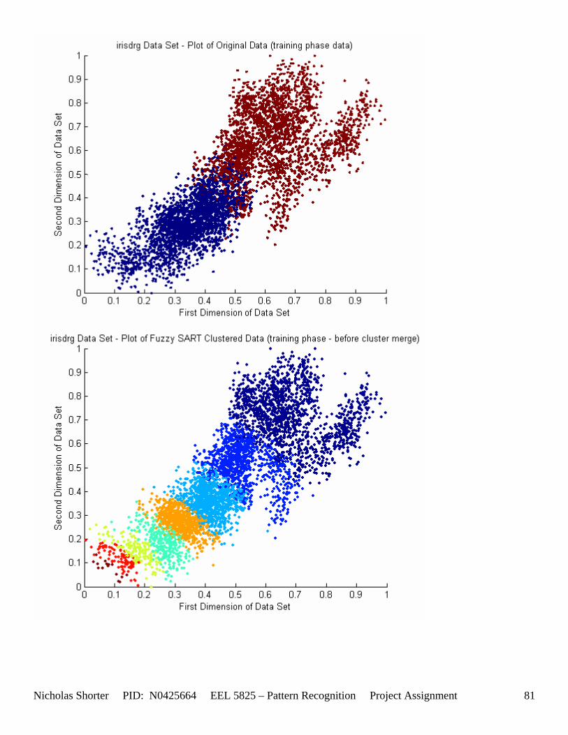
Nicholas Shorter PID: N0425664 EEL 5825 – Pattern Recognition Project Assignment 81
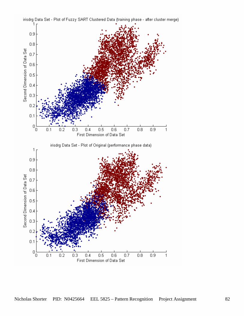
Nicholas Shorter PID: N0425664 EEL 5825 – Pattern Recognition Project Assignment 82
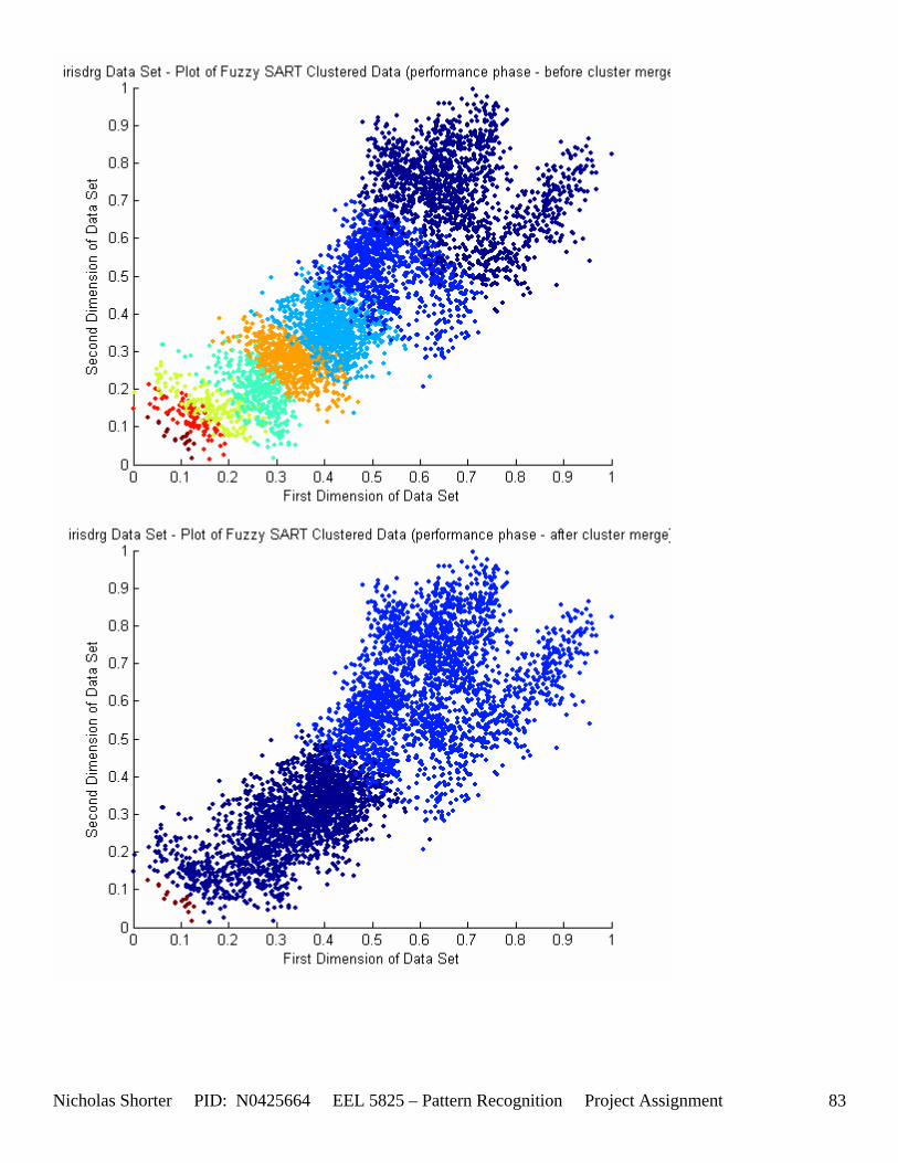
Nicholas Shorter PID: N0425664 EEL 5825 – Pattern Recognition Project Assignment 83
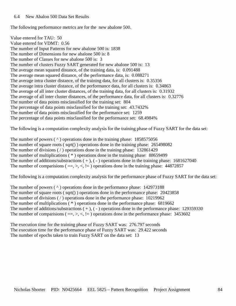
Nicholas Shorter PID: N0425664 EEL 5825 – Pattern Recognition Project Assignment 84
6.4 New Abalon 500 Data Set Results
The following performance metrics are for the new abalone 500. Value entered for TAU: 50 Value entered for VDMT: 0.56 The number of Input Patterns for new abalone 500 is: 1838 The number of Dimensions for new abalone 500 is: 8 The number of Classes for new abalone 500 is: 3 The number of clusters Fuzzy SART generated for new abalone 500 is: 13 The average mean squared distance, of the training data, is: 0.091488 The average mean squared distance, of the performance data, is: 0.088271 The average intra cluster distance, of the training data, for all clusters is: 0.35356 The average intra cluster distance, of the performance data, for all clusters is: 0.34863 The average of all inter cluster distances, of the training data, for all clusters is: 0.31932 The average of all inter cluster distances, of the performance data, for all clusters is: 0.32776 The number of data points misclassified for the training set: 804 The percentage of data points misclassified for the training set: 43.7432% The number of data points misclassified for the performance set: 1259 The percentage of data points misclassified for the performance set: 68.4984% The following is a computation complexity analysis for the training phase of Fuzzy SART for the data set: The number of powers ( ^ ) operations done in the training phase: 1858575056 The number of square roots ( sqrt() ) operations done in the training phase: 265498082 The number of divisions ( / ) operations done in the training phase: 132861429 The number of multiplications ( * ) operations done in the training phase: 88659499 The number of additions/substractions ( + ), ( - ) operations done in the training phase: 1681627040 The number of comparisions ( ==, >, <, != ) operations done in the training phase: 44872857 The following is a computation complexity analysis for the performance phase of Fuzzy SART for the data set: The number of powers ( ^ ) operations done in the performance phase: 142973188 The number of square roots ( sqrt() ) operations done in the performance phase: 20423858 The number of divisions ( / ) operations done in the performance phase: 10219962 The number of multiplications ( * ) operations done in the performance phase: 6819662 The number of additions/substractions ( + ), ( - ) operations done in the performance phase: 129359330 The number of comparisions ( ==, >, <, != ) operations done in the performance phase: 3453602 The execution time for the training phase of Fuzzy SART was: 276.797 seconds The execution time for the performance phase of Fuzzy SART was: 29.422 seconds The number of epochs taken to train Fuzzy SART on the data set: 13
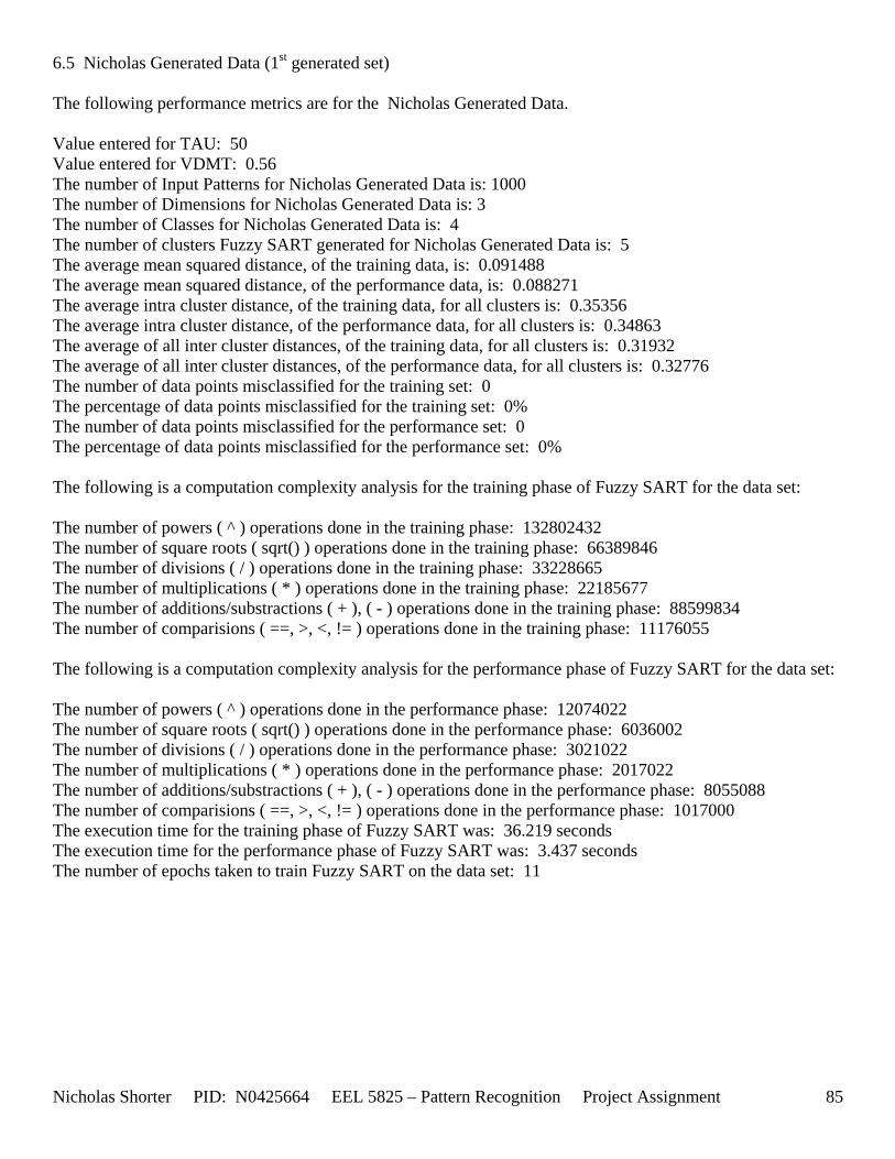
Nicholas Shorter PID: N0425664 EEL 5825 – Pattern Recognition Project Assignment 85
6.5 Nicholas Generated Data (1st generated set) The following performance metrics are for the Nicholas Generated Data. Value entered for TAU: 50 Value entered for VDMT: 0.56 The number of Input Patterns for Nicholas Generated Data is: 1000 The number of Dimensions for Nicholas Generated Data is: 3 The number of Classes for Nicholas Generated Data is: 4 The number of clusters Fuzzy SART generated for Nicholas Generated Data is: 5 The average mean squared distance, of the training data, is: 0.091488 The average mean squared distance, of the performance data, is: 0.088271 The average intra cluster distance, of the training data, for all clusters is: 0.35356 The average intra cluster distance, of the performance data, for all clusters is: 0.34863 The average of all inter cluster distances, of the training data, for all clusters is: 0.31932 The average of all inter cluster distances, of the performance data, for all clusters is: 0.32776 The number of data points misclassified for the training set: 0 The percentage of data points misclassified for the training set: 0% The number of data points misclassified for the performance set: 0 The percentage of data points misclassified for the performance set: 0% The following is a computation complexity analysis for the training phase of Fuzzy SART for the data set: The number of powers ( ^ ) operations done in the training phase: 132802432 The number of square roots ( sqrt() ) operations done in the training phase: 66389846 The number of divisions ( / ) operations done in the training phase: 33228665 The number of multiplications ( * ) operations done in the training phase: 22185677 The number of additions/substractions ( + ), ( - ) operations done in the training phase: 88599834 The number of comparisions ( ==, >, <, != ) operations done in the training phase: 11176055 The following is a computation complexity analysis for the performance phase of Fuzzy SART for the data set: The number of powers ( ^ ) operations done in the performance phase: 12074022 The number of square roots ( sqrt() ) operations done in the performance phase: 6036002 The number of divisions ( / ) operations done in the performance phase: 3021022 The number of multiplications ( * ) operations done in the performance phase: 2017022 The number of additions/substractions ( + ), ( - ) operations done in the performance phase: 8055088 The number of comparisions ( ==, >, <, != ) operations done in the performance phase: 1017000 The execution time for the training phase of Fuzzy SART was: 36.219 seconds The execution time for the performance phase of Fuzzy SART was: 3.437 seconds The number of epochs taken to train Fuzzy SART on the data set: 11
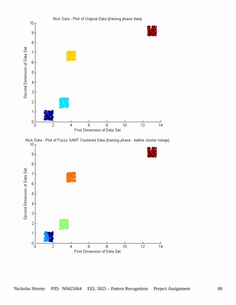
Nicholas Shorter PID: N0425664 EEL 5825 – Pattern Recognition Project Assignment 86
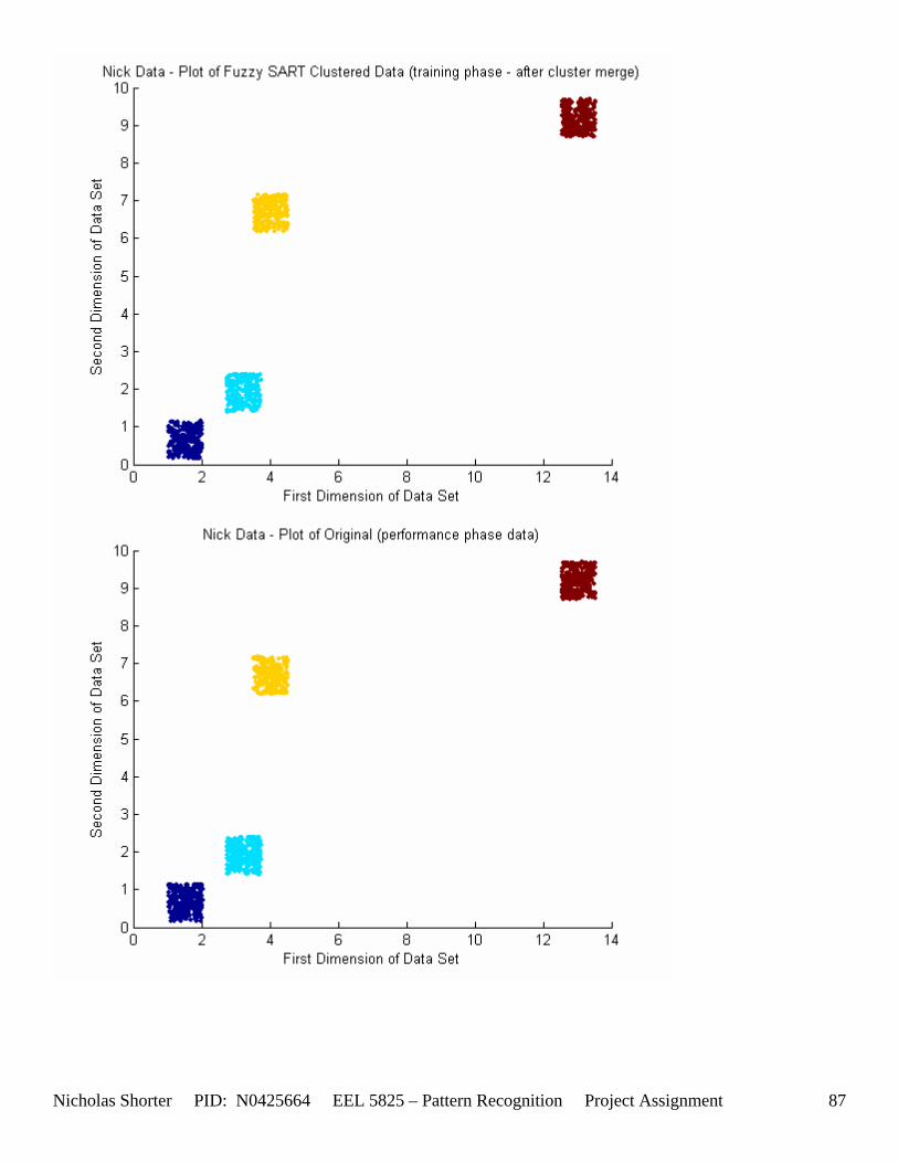
Nicholas Shorter PID: N0425664 EEL 5825 – Pattern Recognition Project Assignment 87
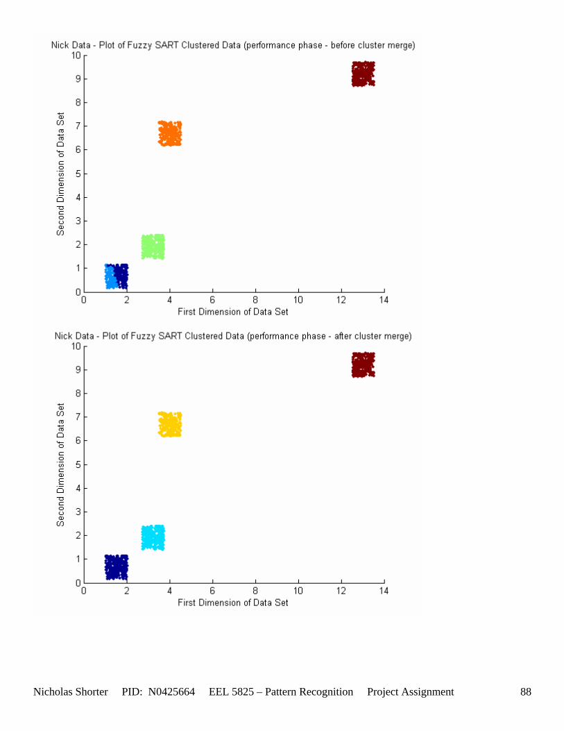
Nicholas Shorter PID: N0425664 EEL 5825 – Pattern Recognition Project Assignment 88
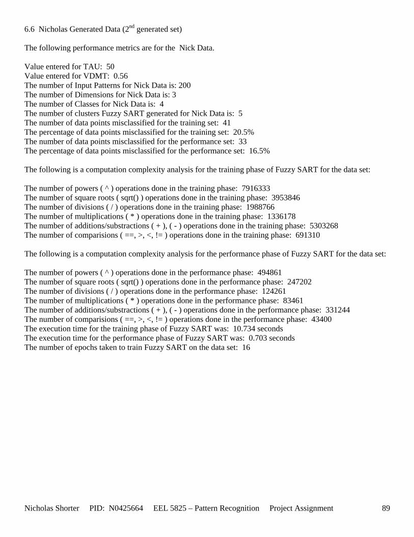
Nicholas Shorter PID: N0425664 EEL 5825 – Pattern Recognition Project Assignment 89
6.6 Nicholas Generated Data (2nd generated set) The following performance metrics are for the Nick Data. Value entered for TAU: 50 Value entered for VDMT: 0.56 The number of Input Patterns for Nick Data is: 200 The number of Dimensions for Nick Data is: 3 The number of Classes for Nick Data is: 4 The number of clusters Fuzzy SART generated for Nick Data is: 5 The number of data points misclassified for the training set: 41 The percentage of data points misclassified for the training set: 20.5% The number of data points misclassified for the performance set: 33 The percentage of data points misclassified for the performance set: 16.5% The following is a computation complexity analysis for the training phase of Fuzzy SART for the data set: The number of powers ( ^ ) operations done in the training phase: 7916333 The number of square roots ( sqrt() ) operations done in the training phase: 3953846 The number of divisions ( / ) operations done in the training phase: 1988766 The number of multiplications ( * ) operations done in the training phase: 1336178 The number of additions/substractions ( + ), ( - ) operations done in the training phase: 5303268 The number of comparisions ( ==, >, <, != ) operations done in the training phase: 691310 The following is a computation complexity analysis for the performance phase of Fuzzy SART for the data set: The number of powers ( ^ ) operations done in the performance phase: 494861 The number of square roots ( sqrt() ) operations done in the performance phase: 247202 The number of divisions ( / ) operations done in the performance phase: 124261 The number of multiplications ( * ) operations done in the performance phase: 83461 The number of additions/substractions ( + ), ( - ) operations done in the performance phase: 331244 The number of comparisions ( ==, >, <, != ) operations done in the performance phase: 43400 The execution time for the training phase of Fuzzy SART was: 10.734 seconds The execution time for the performance phase of Fuzzy SART was: 0.703 seconds The number of epochs taken to train Fuzzy SART on the data set: 16
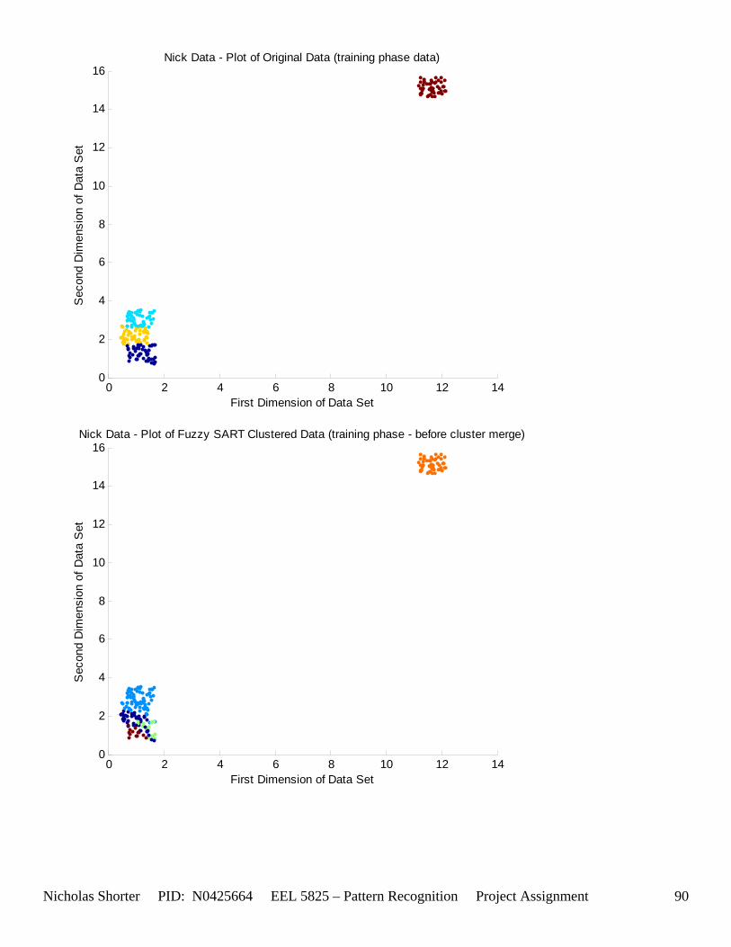
0 2 4 6 8 10 12 140
2
4
6
8
10
12
14
16Nick Data - Plot of Original Data (training phase data)
First Dimension of Data Set
Sec
ond
Dim
ensi
on o
f Dat
a S
et
0 2 4 6 8 10 12 140
2
4
6
8
10
12
14
16Nick Data - Plot of Fuzzy SART Clustered Data (training phase - before cluster merge)
First Dimension of Data Set
Sec
ond
Dim
ensi
on o
f Dat
a S
et
Nicholas Shorter PID: N0425664 EEL 5825 – Pattern Recognition Project Assignment 90
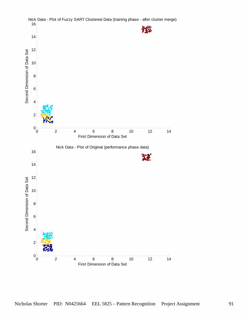
0 2 4 6 8 10 12 140
2
4
6
8
10
12
14
16Nick Data - Plot of Fuzzy SART Clustered Data (training phase - after cluster merge)
First Dimension of Data Set
Sec
ond
Dim
ensi
on o
f Dat
a S
et
0 2 4 6 8 10 12 140
2
4
6
8
10
12
14
16Nick Data - Plot of Original (performance phase data)
First Dimension of Data Set
Sec
ond
Dim
ensi
on o
f Dat
a S
et
Nicholas Shorter PID: N0425664 EEL 5825 – Pattern Recognition Project Assignment 91
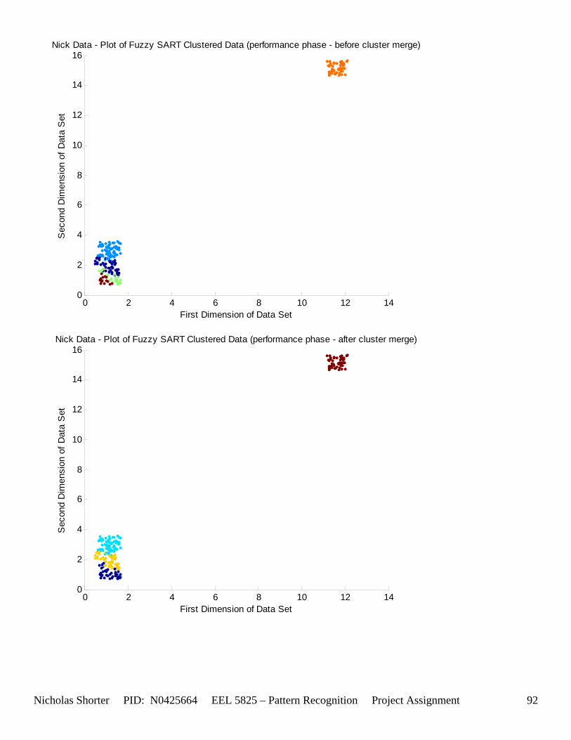
0 2 4 6 8 10 12 140
2
4
6
8
10
12
14
16Nick Data - Plot of Fuzzy SART Clustered Data (performance phase - before cluster merge)
First Dimension of Data Set
Sec
ond
Dim
ensi
on o
f Dat
a S
et
0 2 4 6 8 10 12 140
2
4
6
8
10
12
14
16Nick Data - Plot of Fuzzy SART Clustered Data (performance phase - after cluster merge)
First Dimension of Data Set
Sec
ond
Dim
ensi
on o
f Dat
a S
et
Nicholas Shorter PID: N0425664 EEL 5825 – Pattern Recognition Project Assignment 92
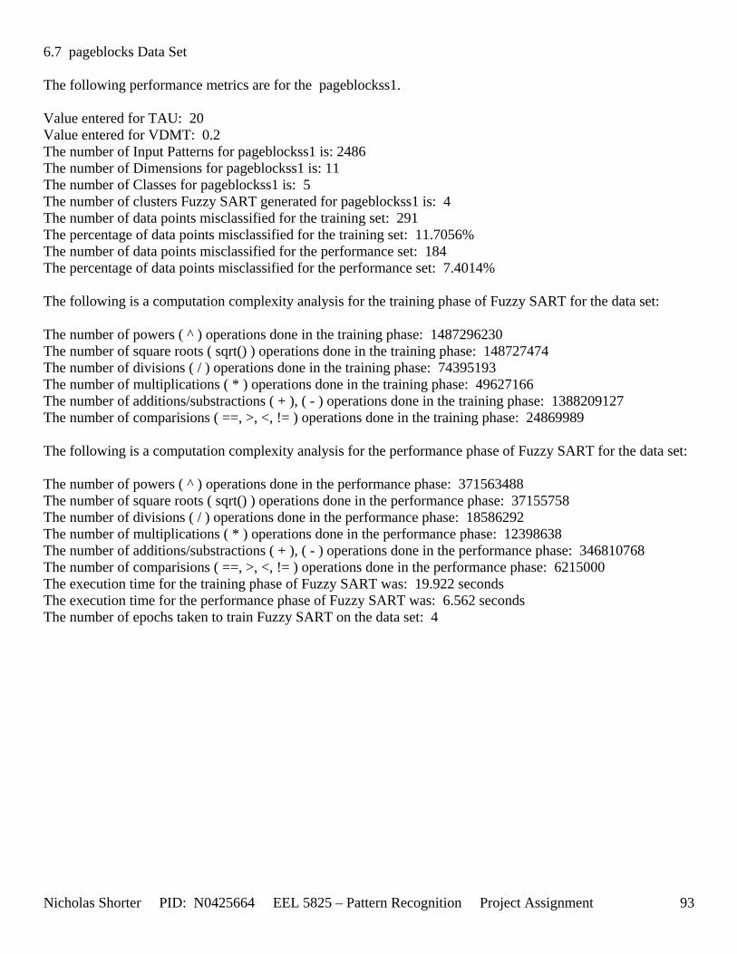
Nicholas Shorter PID: N0425664 EEL 5825 – Pattern Recognition Project Assignment 93
6.7 pageblocks Data Set The following performance metrics are for the pageblockss1. Value entered for TAU: 20 Value entered for VDMT: 0.2 The number of Input Patterns for pageblockss1 is: 2486 The number of Dimensions for pageblockss1 is: 11 The number of Classes for pageblockss1 is: 5 The number of clusters Fuzzy SART generated for pageblockss1 is: 4 The number of data points misclassified for the training set: 291 The percentage of data points misclassified for the training set: 11.7056% The number of data points misclassified for the performance set: 184 The percentage of data points misclassified for the performance set: 7.4014% The following is a computation complexity analysis for the training phase of Fuzzy SART for the data set: The number of powers ( ^ ) operations done in the training phase: 1487296230 The number of square roots ( sqrt() ) operations done in the training phase: 148727474 The number of divisions ( / ) operations done in the training phase: 74395193 The number of multiplications ( * ) operations done in the training phase: 49627166 The number of additions/substractions ( + ), ( - ) operations done in the training phase: 1388209127 The number of comparisions ( ==, >, <, != ) operations done in the training phase: 24869989 The following is a computation complexity analysis for the performance phase of Fuzzy SART for the data set: The number of powers ( ^ ) operations done in the performance phase: 371563488 The number of square roots ( sqrt() ) operations done in the performance phase: 37155758 The number of divisions ( / ) operations done in the performance phase: 18586292 The number of multiplications ( * ) operations done in the performance phase: 12398638 The number of additions/substractions ( + ), ( - ) operations done in the performance phase: 346810768 The number of comparisions ( ==, >, <, != ) operations done in the performance phase: 6215000 The execution time for the training phase of Fuzzy SART was: 19.922 seconds The execution time for the performance phase of Fuzzy SART was: 6.562 seconds The number of epochs taken to train Fuzzy SART on the data set: 4
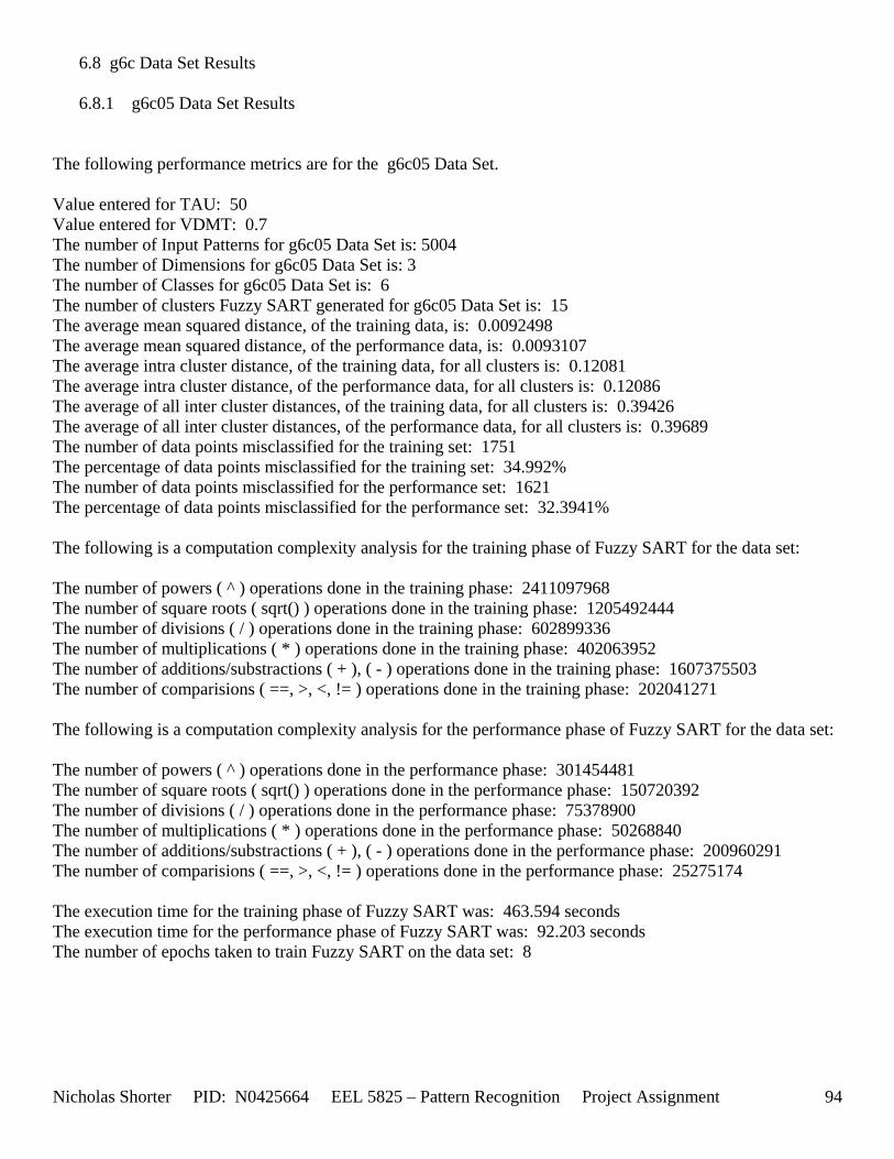
Nicholas Shorter PID: N0425664 EEL 5825 – Pattern Recognition Project Assignment 94
6.8 g6c Data Set Results 6.8.1 g6c05 Data Set Results
The following performance metrics are for the g6c05 Data Set. Value entered for TAU: 50 Value entered for VDMT: 0.7 The number of Input Patterns for g6c05 Data Set is: 5004 The number of Dimensions for g6c05 Data Set is: 3 The number of Classes for g6c05 Data Set is: 6 The number of clusters Fuzzy SART generated for g6c05 Data Set is: 15 The average mean squared distance, of the training data, is: 0.0092498 The average mean squared distance, of the performance data, is: 0.0093107 The average intra cluster distance, of the training data, for all clusters is: 0.12081 The average intra cluster distance, of the performance data, for all clusters is: 0.12086 The average of all inter cluster distances, of the training data, for all clusters is: 0.39426 The average of all inter cluster distances, of the performance data, for all clusters is: 0.39689 The number of data points misclassified for the training set: 1751 The percentage of data points misclassified for the training set: 34.992% The number of data points misclassified for the performance set: 1621 The percentage of data points misclassified for the performance set: 32.3941% The following is a computation complexity analysis for the training phase of Fuzzy SART for the data set: The number of powers ( ^ ) operations done in the training phase: 2411097968 The number of square roots ( sqrt() ) operations done in the training phase: 1205492444 The number of divisions ( / ) operations done in the training phase: 602899336 The number of multiplications ( * ) operations done in the training phase: 402063952 The number of additions/substractions ( + ), ( - ) operations done in the training phase: 1607375503 The number of comparisions ( ==, >, <, != ) operations done in the training phase: 202041271 The following is a computation complexity analysis for the performance phase of Fuzzy SART for the data set: The number of powers ( ^ ) operations done in the performance phase: 301454481 The number of square roots ( sqrt() ) operations done in the performance phase: 150720392 The number of divisions ( / ) operations done in the performance phase: 75378900 The number of multiplications ( * ) operations done in the performance phase: 50268840 The number of additions/substractions ( + ), ( - ) operations done in the performance phase: 200960291 The number of comparisions ( ==, >, <, != ) operations done in the performance phase: 25275174 The execution time for the training phase of Fuzzy SART was: 463.594 seconds The execution time for the performance phase of Fuzzy SART was: 92.203 seconds The number of epochs taken to train Fuzzy SART on the data set: 8
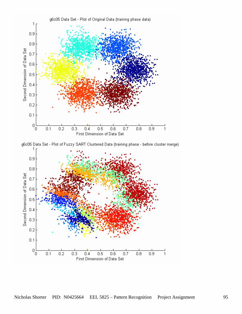
Nicholas Shorter PID: N0425664 EEL 5825 – Pattern Recognition Project Assignment 95
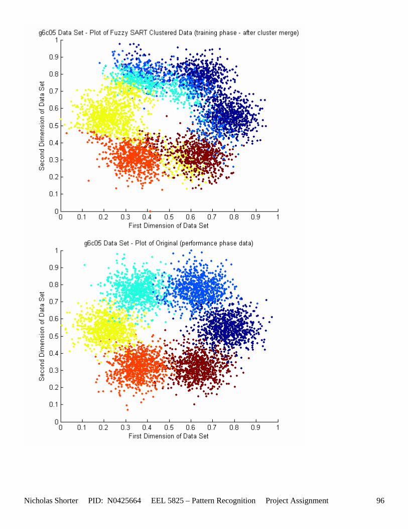
Nicholas Shorter PID: N0425664 EEL 5825 – Pattern Recognition Project Assignment 96
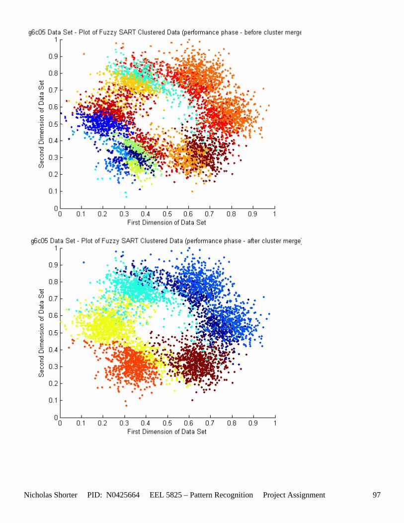
Nicholas Shorter PID: N0425664 EEL 5825 – Pattern Recognition Project Assignment 97
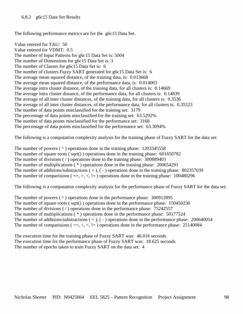
Nicholas Shorter PID: N0425664 EEL 5825 – Pattern Recognition Project Assignment 98
6.8.2 g6c15 Data Set Results The following performance metrics are for the g6c15 Data Set. Value entered for TAU: 50 Value entered for VDMT: 0.5 The number of Input Patterns for g6c15 Data Set is: 5004 The number of Dimensions for g6c15 Data Set is: 3 The number of Classes for g6c15 Data Set is: 6 The number of clusters Fuzzy SART generated for g6c15 Data Set is: 6 The average mean squared distance, of the training data, is: 0.013668 The average mean squared distance, of the performance data, is: 0.014003 The average intra cluster distance, of the training data, for all clusters is: 0.14669 The average intra cluster distance, of the performance data, for all clusters is: 0.14839 The average of all inter cluster distances, of the training data, for all clusters is: 0.3536 The average of all inter cluster distances, of the performance data, for all clusters is: 0.35523 The number of data points misclassified for the training set: 3179 The percentage of data points misclassified for the training set: 63.5292% The number of data points misclassified for the performance set: 3168 The percentage of data points misclassified for the performance set: 63.3094% The following is a computation complexity analysis for the training phase of Fuzzy SART for the data set: The number of powers ( ^ ) operations done in the training phase: 1203345558 The number of square roots ( sqrt() ) operations done in the training phase: 601650782 The number of divisions ( / ) operations done in the training phase: 300889403 The number of multiplications ( * ) operations done in the training phase: 200654291 The number of additions/substractions ( + ), ( - ) operations done in the training phase: 802357039 The number of comparisions ( ==, >, <, != ) operations done in the training phase: 100480296 The following is a computation complexity analysis for the performance phase of Fuzzy SART for the data set: The number of powers ( ^ ) operations done in the performance phase: 300912895 The number of square roots ( sqrt() ) operations done in the performance phase: 150450230 The number of divisions ( / ) operations done in the performance phase: 75242557 The number of multiplications ( * ) operations done in the performance phase: 50177524 The number of additions/substractions ( + ), ( - ) operations done in the performance phase: 200640054 The number of comparisions ( ==, >, <, != ) operations done in the performance phase: 25140084 The execution time for the training phase of Fuzzy SART was: 46.016 seconds The execution time for the performance phase of Fuzzy SART was: 18.625 seconds The number of epochs taken to train Fuzzy SART on the data set: 4
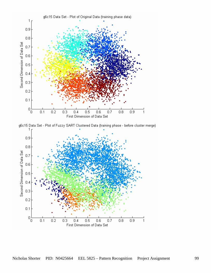
Nicholas Shorter PID: N0425664 EEL 5825 – Pattern Recognition Project Assignment 99
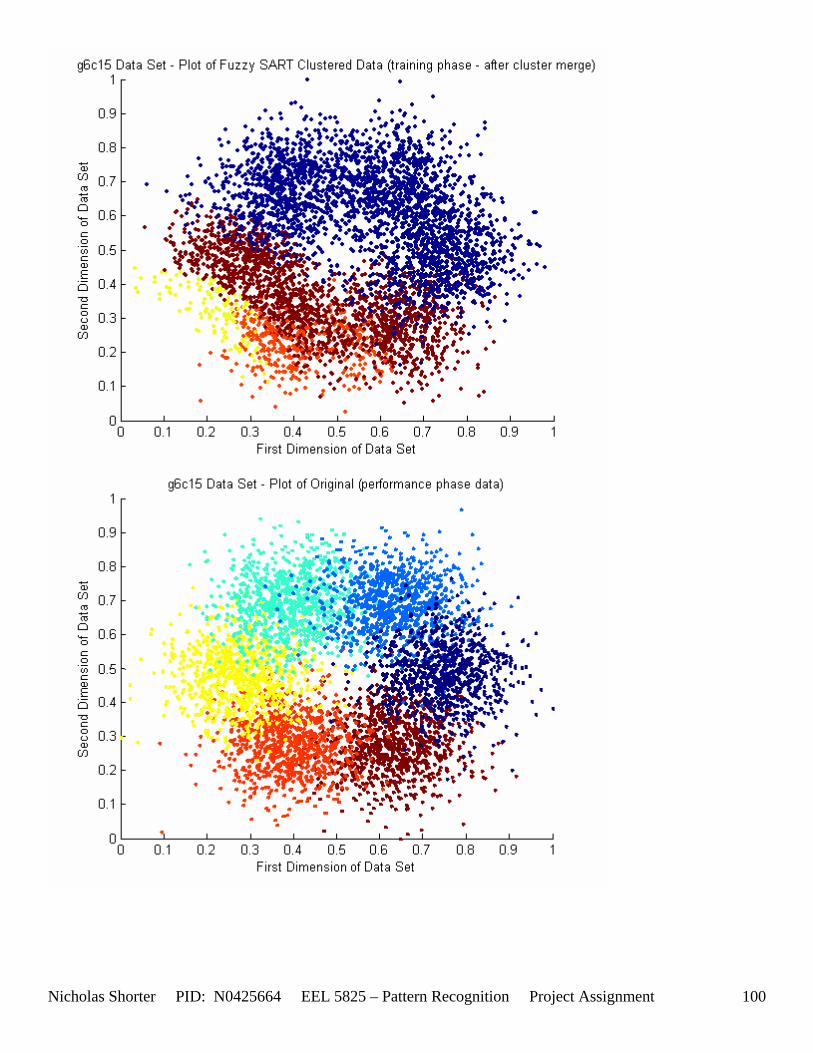
Nicholas Shorter PID: N0425664 EEL 5825 – Pattern Recognition Project Assignment 100
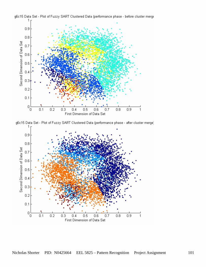
Nicholas Shorter PID: N0425664 EEL 5825 – Pattern Recognition Project Assignment 101
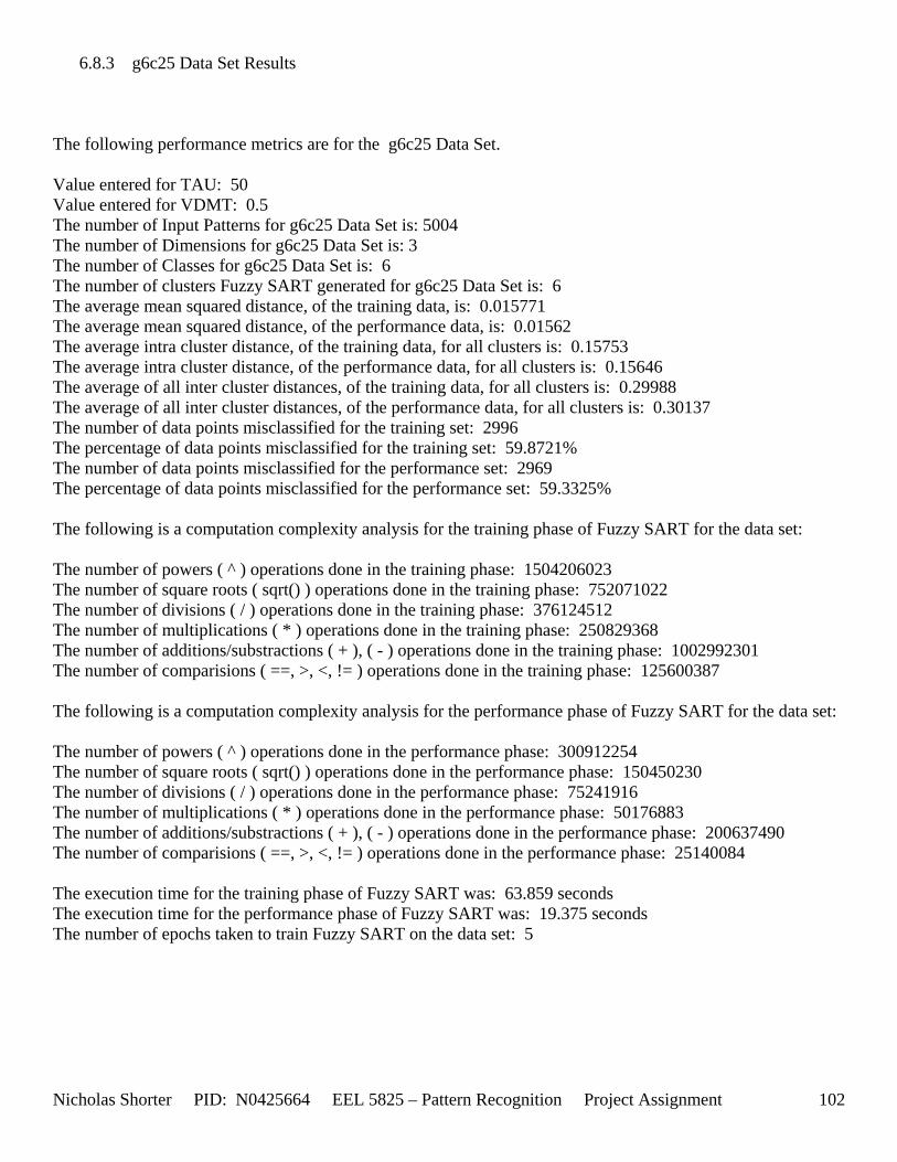
Nicholas Shorter PID: N0425664 EEL 5825 – Pattern Recognition Project Assignment 102
6.8.3 g6c25 Data Set Results The following performance metrics are for the g6c25 Data Set. Value entered for TAU: 50 Value entered for VDMT: 0.5 The number of Input Patterns for g6c25 Data Set is: 5004 The number of Dimensions for g6c25 Data Set is: 3 The number of Classes for g6c25 Data Set is: 6 The number of clusters Fuzzy SART generated for g6c25 Data Set is: 6 The average mean squared distance, of the training data, is: 0.015771 The average mean squared distance, of the performance data, is: 0.01562 The average intra cluster distance, of the training data, for all clusters is: 0.15753 The average intra cluster distance, of the performance data, for all clusters is: 0.15646 The average of all inter cluster distances, of the training data, for all clusters is: 0.29988 The average of all inter cluster distances, of the performance data, for all clusters is: 0.30137 The number of data points misclassified for the training set: 2996 The percentage of data points misclassified for the training set: 59.8721% The number of data points misclassified for the performance set: 2969 The percentage of data points misclassified for the performance set: 59.3325% The following is a computation complexity analysis for the training phase of Fuzzy SART for the data set: The number of powers ( ^ ) operations done in the training phase: 1504206023 The number of square roots ( sqrt() ) operations done in the training phase: 752071022 The number of divisions ( / ) operations done in the training phase: 376124512 The number of multiplications ( * ) operations done in the training phase: 250829368 The number of additions/substractions ( + ), ( - ) operations done in the training phase: 1002992301 The number of comparisions ( ==, >, <, != ) operations done in the training phase: 125600387 The following is a computation complexity analysis for the performance phase of Fuzzy SART for the data set: The number of powers ( ^ ) operations done in the performance phase: 300912254 The number of square roots ( sqrt() ) operations done in the performance phase: 150450230 The number of divisions ( / ) operations done in the performance phase: 75241916 The number of multiplications ( * ) operations done in the performance phase: 50176883 The number of additions/substractions ( + ), ( - ) operations done in the performance phase: 200637490 The number of comparisions ( ==, >, <, != ) operations done in the performance phase: 25140084 The execution time for the training phase of Fuzzy SART was: 63.859 seconds The execution time for the performance phase of Fuzzy SART was: 19.375 seconds The number of epochs taken to train Fuzzy SART on the data set: 5
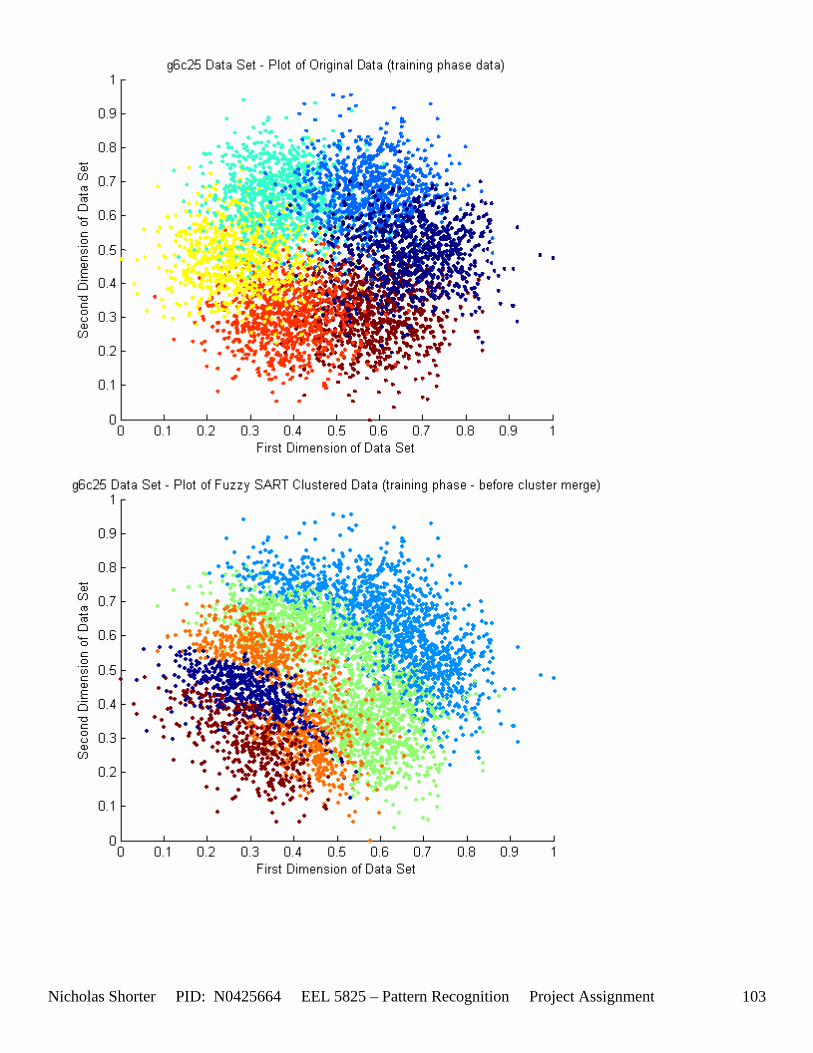
Nicholas Shorter PID: N0425664 EEL 5825 – Pattern Recognition Project Assignment 103
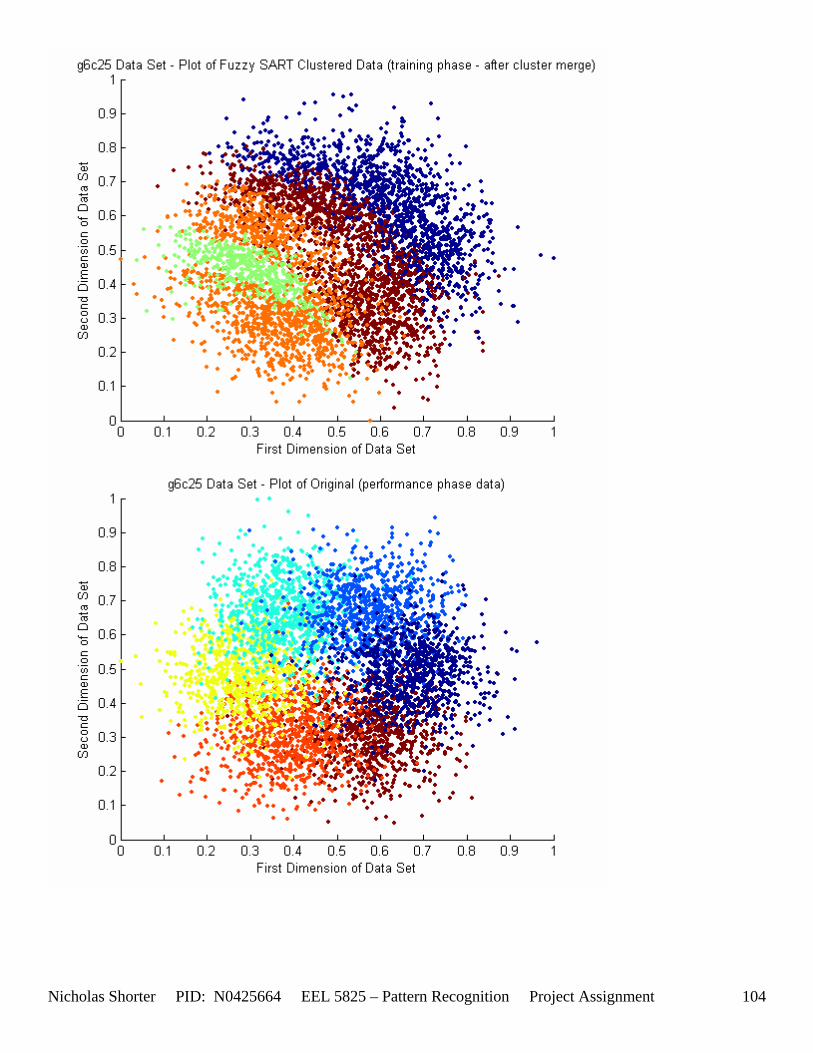
Nicholas Shorter PID: N0425664 EEL 5825 – Pattern Recognition Project Assignment 104
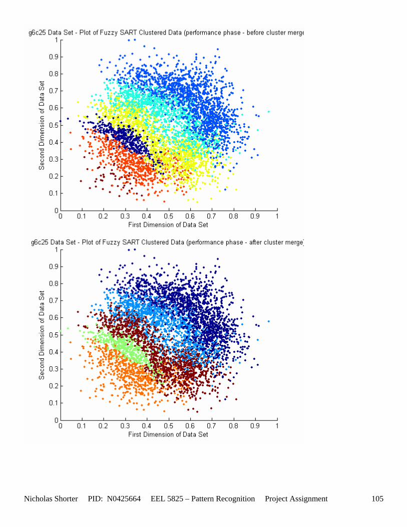
Nicholas Shorter PID: N0425664 EEL 5825 – Pattern Recognition Project Assignment 105
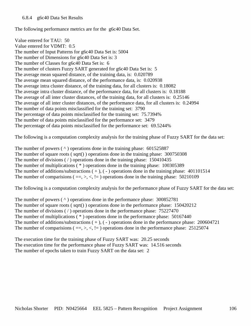
Nicholas Shorter PID: N0425664 EEL 5825 – Pattern Recognition Project Assignment 106
6.8.4 g6c40 Data Set Results The following performance metrics are for the g6c40 Data Set. Value entered for TAU: 50 Value entered for VDMT: 0.5 The number of Input Patterns for g6c40 Data Set is: 5004 The number of Dimensions for g6c40 Data Set is: 3 The number of Classes for g6c40 Data Set is: 6 The number of clusters Fuzzy SART generated for g6c40 Data Set is: 5 The average mean squared distance, of the training data, is: 0.020789 The average mean squared distance, of the performance data, is: 0.020938 The average intra cluster distance, of the training data, for all clusters is: 0.18082 The average intra cluster distance, of the performance data, for all clusters is: 0.18188 The average of all inter cluster distances, of the training data, for all clusters is: 0.25146 The average of all inter cluster distances, of the performance data, for all clusters is: 0.24994 The number of data points misclassified for the training set: 3790 The percentage of data points misclassified for the training set: 75.7394% The number of data points misclassified for the performance set: 3479 The percentage of data points misclassified for the performance set: 69.5244% The following is a computation complexity analysis for the training phase of Fuzzy SART for the data set: The number of powers ( ^ ) operations done in the training phase: 601525887 The number of square roots ( sqrt() ) operations done in the training phase: 300750308 The number of divisions ( / ) operations done in the training phase: 150410435 The number of multiplications ( * ) operations done in the training phase: 100305389 The number of additions/substractions ( + ), ( - ) operations done in the training phase: 401101514 The number of comparisions ( ==, >, <, != ) operations done in the training phase: 50210109 The following is a computation complexity analysis for the performance phase of Fuzzy SART for the data set: The number of powers ( ^ ) operations done in the performance phase: 300852781 The number of square roots ( sqrt() ) operations done in the performance phase: 150420212 The number of divisions ( / ) operations done in the performance phase: 75227470 The number of multiplications ( * ) operations done in the performance phase: 50167440 The number of additions/substractions ( + ), ( - ) operations done in the performance phase: 200604721 The number of comparisions ( ==, >, <, != ) operations done in the performance phase: 25125074 The execution time for the training phase of Fuzzy SART was: 20.25 seconds The execution time for the performance phase of Fuzzy SART was: 14.516 seconds The number of epochs taken to train Fuzzy SART on the data set: 2
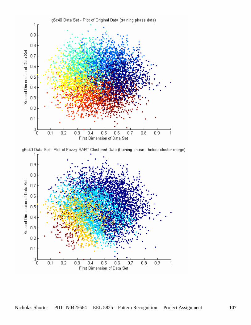
Nicholas Shorter PID: N0425664 EEL 5825 – Pattern Recognition Project Assignment 107
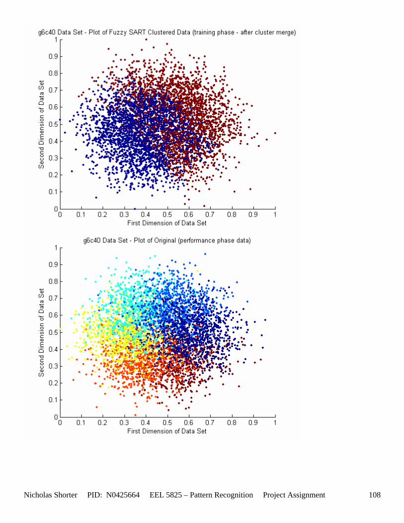
Nicholas Shorter PID: N0425664 EEL 5825 – Pattern Recognition Project Assignment 108
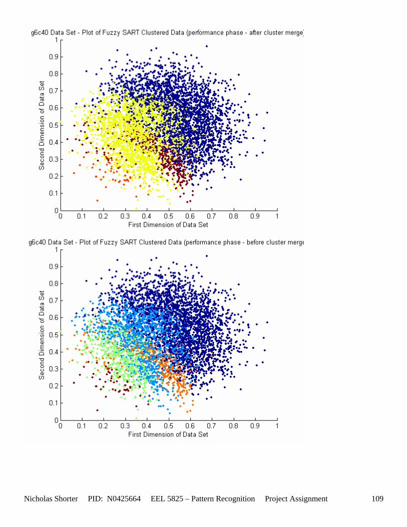
Nicholas Shorter PID: N0425664 EEL 5825 – Pattern Recognition Project Assignment 109
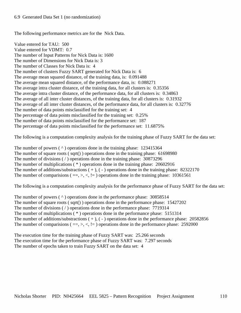
Nicholas Shorter PID: N0425664 EEL 5825 – Pattern Recognition Project Assignment 110
6.9 Generated Data Set 1 (no randomization) The following performance metrics are for the Nick Data. Value entered for TAU: 500 Value entered for VDMT: 0.7 The number of Input Patterns for Nick Data is: 1600 The number of Dimensions for Nick Data is: 3 The number of Classes for Nick Data is: 4 The number of clusters Fuzzy SART generated for Nick Data is: 6 The average mean squared distance, of the training data, is: 0.091488 The average mean squared distance, of the performance data, is: 0.088271 The average intra cluster distance, of the training data, for all clusters is: 0.35356 The average intra cluster distance, of the performance data, for all clusters is: 0.34863 The average of all inter cluster distances, of the training data, for all clusters is: 0.31932 The average of all inter cluster distances, of the performance data, for all clusters is: 0.32776 The number of data points misclassified for the training set: 4 The percentage of data points misclassified for the training set: 0.25% The number of data points misclassified for the performance set: 187 The percentage of data points misclassified for the performance set: 11.6875% The following is a computation complexity analysis for the training phase of Fuzzy SART for the data set: The number of powers ( ^ ) operations done in the training phase: 123415364 The number of square roots ( sqrt() ) operations done in the training phase: 61698980 The number of divisions ( / ) operations done in the training phase: 30873296 The number of multiplications ( * ) operations done in the training phase: 20602916 The number of additions/substractions ( + ), ( - ) operations done in the training phase: 82322170 The number of comparisions ( ==, >, <, != ) operations done in the training phase: 10361561 The following is a computation complexity analysis for the performance phase of Fuzzy SART for the data set: The number of powers ( ^ ) operations done in the performance phase: 30858514 The number of square roots ( sqrt() ) operations done in the performance phase: 15427202 The number of divisions ( / ) operations done in the performance phase: 7719314 The number of multiplications ( * ) operations done in the performance phase: 5151314 The number of additions/substractions ( + ), ( - ) operations done in the performance phase: 20582856 The number of comparisions ( ==, >, <, != ) operations done in the performance phase: 2592000 The execution time for the training phase of Fuzzy SART was: 25.266 seconds The execution time for the performance phase of Fuzzy SART was: 7.297 seconds The number of epochs taken to train Fuzzy SART on the data set: 4
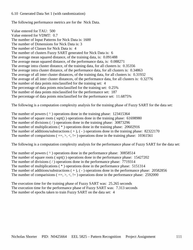
Nicholas Shorter PID: N0425664 EEL 5825 – Pattern Recognition Project Assignment 111
6.10 Generated Data Set 1 (with randomization) The following performance metrics are for the Nick Data. Value entered for TAU: 500 Value entered for VDMT: 0.7 The number of Input Patterns for Nick Data is: 1600 The number of Dimensions for Nick Data is: 3 The number of Classes for Nick Data is: 4 The number of clusters Fuzzy SART generated for Nick Data is: 6 The average mean squared distance, of the training data, is: 0.091488 The average mean squared distance, of the performance data, is: 0.088271 The average intra cluster distance, of the training data, for all clusters is: 0.35356 The average intra cluster distance, of the performance data, for all clusters is: 0.34863 The average of all inter cluster distances, of the training data, for all clusters is: 0.31932 The average of all inter cluster distances, of the performance data, for all clusters is: 0.32776 The number of data points misclassified for the training set: 4 The percentage of data points misclassified for the training set: 0.25% The number of data points misclassified for the performance set: 187 The percentage of data points misclassified for the performance set: 11.6875% The following is a computation complexity analysis for the training phase of Fuzzy SART for the data set: The number of powers ( ^ ) operations done in the training phase: 123415364 The number of square roots ( sqrt() ) operations done in the training phase: 61698980 The number of divisions ( / ) operations done in the training phase: 30873296 The number of multiplications ( * ) operations done in the training phase: 20602916 The number of additions/substractions ( + ), ( - ) operations done in the training phase: 82322170 The number of comparisions ( ==, >, <, != ) operations done in the training phase: 10361561 The following is a computation complexity analysis for the performance phase of Fuzzy SART for the data set: The number of powers ( ^ ) operations done in the performance phase: 30858514 The number of square roots ( sqrt() ) operations done in the performance phase: 15427202 The number of divisions ( / ) operations done in the performance phase: 7719314 The number of multiplications ( * ) operations done in the performance phase: 5151314 The number of additions/substractions ( + ), ( - ) operations done in the performance phase: 20582856 The number of comparisions ( ==, >, <, != ) operations done in the performance phase: 2592000 The execution time for the training phase of Fuzzy SART was: 25.265 seconds The execution time for the performance phase of Fuzzy SART was: 7.313 seconds The number of epochs taken to train Fuzzy SART on the data set: 4

Nicholas Shorter PID: N0425664 EEL 5825 – Pattern Recognition Project Assignment 112
7 Appendix 7 – Matlab Code The data set results appendix section is composed of the following sections:
7.1 Note on proj_x template 7.2 fsart.m – training phase MATLAB function 7.3 pfsart.m – performance phase MATLAB function
A note about the proj_x templates: All of the data presented in the previous appendix section of this report can be reproduced by running each of the following data set template script files corresponding to each data set: Name of Data Set
Corresponding MATLAB Project Template File
g2c_05 proj_1 g2c_15 proj_2 g2c_25 proj_3 g2c_40 proj_4 g4c_05 proj_5 g4c_15 proj_6 g4c_25 proj_7 g4c_40 proj_8 g6c_05 proj_9 g6c_15 proj_10 g6c_25 proj_11 g6c_40 proj_12 iris_drg proj_13 new_abalone_500 proj_14 pageblocks proj_15 There are several functions called from the project template file, one of which being the Fuzzy SART MATLAB implementation function file. From the Fuzzy SART implementation function file, several other functions are called from it. All of these function have been tediously commented and provided in the enclosed CD. For those who do not have MATLAB, the code has been copied to a word file named APPENDIX_CODE.DOC. Only the Fuzzy SART training and performance functions are presented in this portion of the appendix. A mapping of how all the implemented functions for this project relate to one another is provided in the following [Figure 2]. The MATLAB file proj_g was used to generate outputs for the generated data. The MATLAB file proj_gr.m was used to randomize the input order and look for any changes in performance.
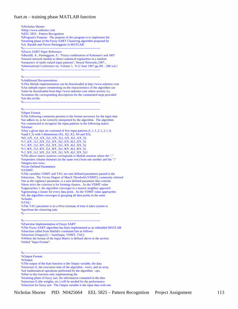
Nicholas Shorter PID: N0425664 EEL 5825 – Pattern Recognition Project Assignment 113
fsart.m – training phase MATLAB function
%Nicholas Shorter %http://www.nshorter.com %EEL 5825 - Pattern Recognition %Program's Purpose: The purpose of this program is to implement the %training phase of the Fuzzy SART Clustering algorithm proposed by %A. Baraldi and Flavio Parmiggiani in MATLAB. %-------------------------------------------------------------------------- %Fuzzy SART Paper Reference: %Baraldi, A.; Parmiggiani, F.; “Fuzzy combination of Kohonen's and ART %neural network models to detect statistical regularities in a random %sequence of multi-valued input patterns”, Neural Networks,1997., %International Conference on, Volume 1, 9-12 June 1997 pp.281 - 286 vol.1 %-------------------------------------------------------------------------- %-------------------------------------------------------------------------- %Additional Documentation: %This Matlab implementation can be downloaded at http://www.nshorter.com %An indepth report commenting on the characteristics of the algorithm can %also be downloaded from http://www.nshorter.com where section 3.a. %contains the corresponding descriptions for the commented steps provided %in this m-file. %-------------------------------------------------------------------------- %-------------------------------------------------------------------------- %Input Format: %The following comments pertains to the format necessary for the input data %to adhere to, to be correctly intrepreted by the algorithm. The algorithm %is constructed to recognize the input patterns in the following matrix %format: %Say a given data set consisted of five input patterns (I_1, I_2, I_3, I_4, %and I_5) with 5 dimensions (X1, X2, X3, X4 and X5). %[I_1(X_1),I_1(X_2),I_1(X_3),I_1(X_4),I_1(X_5); % I_2(X_1),I_2(X_2),I_2(X_3),I_2(X_4),I_2(X_5); % I_3(X_1),I_3(X_2),I_3(X_3),I_3(X_4),I_3(X_5); % I_4(X_1),I_4(X_2),I_4(X_3),I_4(X_4),I_4(X_5); % I_5(X_1),I_5(X_2),I_5(X_3),I_5(X_4),I_5(X_5);] %The above matrix notation corresponds to Matlab notation where the "," %seperates column elements (in the same row) from one another and the ";" %begins new rows. %User Defined Parameters: %VDMT: %The variables VDMT and TAU are user defined parameters passed to the %function. The Vector Degree of Match Threshold (VDMT), commonly referred %to as the vigilance parameter, is a user defined parameter that controls %how strict the criterion is for forming clusters. As the VDMT value %approaches 1, the algorithm converges to a nearest neighbor approach %generating a cluster for every data point. As the VDMT value approaches %0, the algorithm converges to grouping all data points in the same %cluster. %TAU: %The TAU parameter is an a-Prioi estimate of time it takes system to %perform the clustering task. %-------------------------------------------------------------------------- %-------------------------------------------------------------------------- %Function Implementation of Fuzzy SART %The Fuzzy SART algorithm has been implemented as an imbedded MATLAB %function called from Matlab's command line as follows: %function [Output,E] = fsart(Input, VDMT, TAU) %Where the format of the Input Matrix is defined above in the section %titled "Input Format". %-------------------------------------------------------------------------- %Output Format: %Output: %The output of the fsart function is the Output variable, the data %structure E, the execution time of the algorithm - exect, and an array %of mathematical operations performed by the algorithm - ops. %Due to this function only implementing the %training phase of fuzzy sart, the information contained in the data %structure E (the weights, etc.) will be needed for the performance %function for fuzzy sart. The Output variable is the input data with one
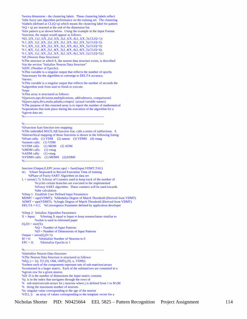
Nicholas Shorter PID: N0425664 EEL 5825 – Pattern Recognition Project Assignment 114
%extra dimension - the clustering labels. These clustering labels reflect %the fuzzy sart algorithm performance on the training set. The clustering %labels (defined as CL(Q=q) which means the clustering label for pattern %Q = q) are inserted at the end of the dimension list %for pattern q as shown below. Using the example in the Input Format %section, the output would appear as follows: %[I_1(X_1),I_1(X_2),I_1(X_3),I_1(X_4),I_1(X_5),CL(Q=1); % I_2(X_1),I_2(X_2),I_2(X_3),I_2(X_4),I_2(X_5),CL(Q=2); % I_3(X_1),I_3(X_2),I_3(X_3),I_3(X_4),I_3(X_5),CL(Q=3); % I_4(X_1),I_4(X_2),I_4(X_3),I_4(X_4),I_4(X_5),CL(Q=4); % I_5(X_1),I_5(X_2),I_5(X_3),I_5(X_4),I_5(X_5),CL(Q=5);] %E (Neuron Data Structure): %The structure in which E, the neuron data structure exists, is described %in the section "Initialize Neuron Data Structure" %EPC (Number of Epochs): %This variable is a singular output that reflects the number of epochs %necessary for the algorithm to converge to DELTA accuracy. %texec: %This variable is a singular output that reflects the number of seconds the %algorithm took from start to finish to execute. %ops: %This array is structured as follows: %[powers,sqrt,divisions,multiplications, add/subtracts, comparisons] %[pwrs,sqrts,divs,mults,adsubs,comprs] (actual variable names) %The purpose of this returned array is to report the number of mathematical %operations that took place during the execution of the algorithm for a %given data set. %-------------------------------------------------------------------------- %-------------------------------------------------------------------------- %Function fsart function tree mapping: %The imbedded MATLAB function fsat, calls a series of subfuctions. A %hierarchical mapping of those functions is shown in the following listing: %Fsart calls: (1) VDM (2) umem (3) VDMS (4) vmag %umem calls: (1) VDM %VDM calls: (1) MDM (2) ADM %MDM calls: (1) vmag %ADM calls: (1) vmag %VDMS calls: (1) MDMS (2)ADMS %-------------------------------------------------------------------------- function [Output,E,EPC,texec,ops] = fsart(Input,VDMT,TAU) tic; %Start Stopwatch to Record Execution Time of training %Phase of Fuzzy SART Algorithm on data set L = zeros(1,7); %Array of Counters used to keep track of the number of %cycles certain branches are executed in the implemented %Fuzzy SART algorithm. These counters will be used towards %the calculation %Step 1: Establish User Defined Input Parameters MDMT = sqrt(VDMT); %Modulus Degree of Match Threshold (Derived from VDMT) ADMT = sqrt(VDMT); %Angle Degree of Match Threshold (Derived from VDMT) DELTA = 0.1; %Convergence Parameter defined by application developer %Step 2: Initialize Algorithm Parameters X = Input; %Setting X equal to Input to keep nomenclature similiar to %what is used in referened paper [Q,D] = size(X); %Q = Number of Input Patterns %D = Number of Dimensions of Input Patterns Output = zeros(Q,D+1); M = 0; %Initialize Number of Neurons to 0 EPC = 0; %Initialize Epochs to 1 %-------------------------------------------------------------------------- %Initialize Neuron Data Structure: %The Neuron Data Structure is structured as follows: %E(j,:) = {t), T(1,D), Oldt, OldT(j,D), u, VDM)} %where each of the components represent sets of sub-matrixes/arrays %contained in a larger matrix. Each of the submatrixes are contained in a %given row for a given neuron. %D: D is the number of dimensions the Input matrix contains %j: is in the index that navigates through the rows of % sub-matrixes/sub-arrays for j neurons where j is defined from 1 to M (M % being the maximum number of neurons. %t: singular value corresponding to the age of the neuron %T(1,:): an array of values corresponding to the template vector for a
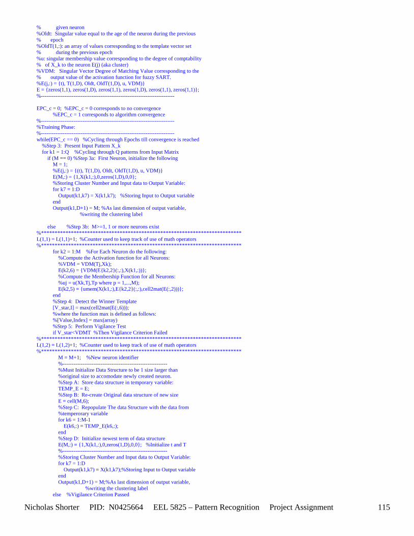
Nicholas Shorter PID: N0425664 EEL 5825 – Pattern Recognition Project Assignment 115
% given neuron %Oldt: Singular value equal to the age of the neuron during the previous % epoch %OldT(1,:): an array of values corresponding to the template vector set % during the previous epoch %u: singular membership value corresponding to the degree of comptability % of X_k to the neuron E(j) (aka cluster) %VDM: Singular Vector Degree of Matching Value corresponding to the % output value of the activation function for fuzzy SART. %E(j,:) = {t), T(1,D), Oldt, OldT(1,D), u, VDM)} E = {zeros(1,1), zeros(1,D), zeros(1,1), zeros(1,D), zeros(1,1), zeros(1,1)}; %-------------------------------------------------------------------------- EPC_c = 0; %EPC_c = 0 corresponds to no convergence %EPC_c = 1 corresponds to algorithm convergence %-------------------------------------------------------------------------- %Training Phase: %-------------------------------------------------------------------------- while(EPC_c == 0) %Cycling through Epochs till convergence is reached %Step 3: Present Input Pattern X_k for k1 = 1:Q %Cycling through Q patterns from Input Matrix if (M == 0) %Step 3a: First Neuron, initialize the following M = 1; %E(j,:) = {(t), T(1,D), Oldt, OldT(1,D), u, VDM)} E(M,:) = {1,X(k1,:),0,zeros(1,D),0,0}; %Storing Cluster Number and Input data to Output Variable: for k7 = 1:D Output(k1,k7) = X(k1,k7); %Storing Input to Output variable end Output(k1,D+1) = M; %As last dimension of output variable, %writing the clustering label else %Step 3b: M>=1, 1 or more neurons exist %************************************************************************** L(1,1) = L(1,1)+1; %Counter used to keep track of use of math operators %************************************************************************** for k2 = 1:M %For Each Neuron do the following: %Compute the Activation function for all Neurons: %VDM = VDM(Tj,Xk); E(k2,6) = {VDM(E{k2,2}(:,:),X(k1,:))}; %Compute the Membership Function for all Neurons: %uj = u(Xk,Tj,Tp where p = 1,...,M); E(k2,5) = {umem(X(k1,:),E{k2,2}(:,:),cell2mat(E(:,2)))}; end %Step 4: Detect the Winner Template [V_star,I] = max(cell2mat(E(:,6))); %where the function max is defined as follows: %[Value,Index] = max(array) %Step 5: Perform Vigilance Test if V_star<VDMT %Then Vigilance Criterion Failed %************************************************************************** L(1,2) = L(1,2)+1; %Counter used to keep track of use of math operators %************************************************************************** M = M+1; %New neuron identifier %---------------------------------------------------------- %Must Initialize Data Structure to be 1 size larger than %original size to accomodate newly created neuron. %Step A: Store data structure in temporary variable: TEMP_E = E; %Step B: Re-create Original data structure of new size E = cell(M,6); %Step C: Repopulate The data Structure with the data from %temperorary variable for k6 = 1:M-1 E(k6,:) = TEMP_E(k6,:); end %Step D: Initialize newest term of data structure E(M,:) = {1,X(k1,:),0,zeros(1,D),0,0}; %Initialize t and T %---------------------------------------------------------- %Storing Cluster Number and Input data to Output Variable: for k7 = 1:D Output(k1,k7) = X(k1,k7);%Storing Input to Output variable end Output(k1,D+1) = M;%As last dimension of output variable, %writing the clustering label else %Vigilance Criterion Passed
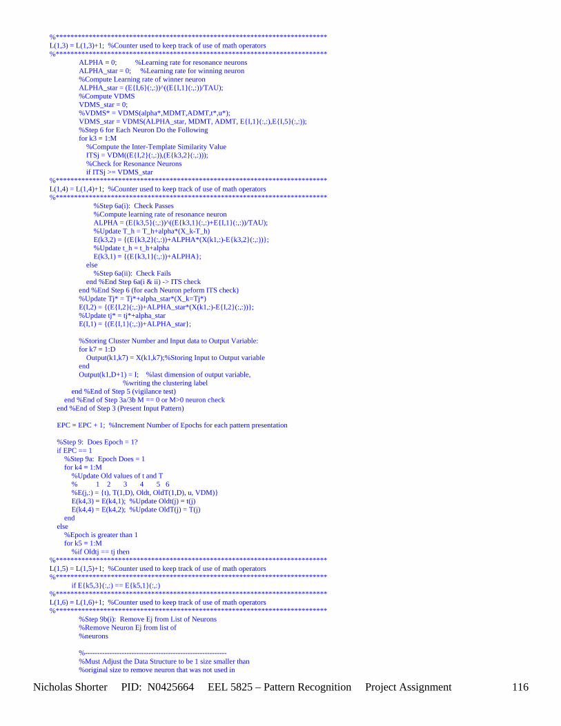
Nicholas Shorter PID: N0425664 EEL 5825 – Pattern Recognition Project Assignment 116
%************************************************************************** L(1,3) = L(1,3)+1; %Counter used to keep track of use of math operators %************************************************************************** ALPHA = 0; %Learning rate for resonance neurons ALPHA_star = 0; %Learning rate for winning neuron %Compute Learning rate of winner neuron ALPHA_star = (E{I,6}(:,:))^((E{I,1}(:,:))/TAU); %Compute VDMS VDMS_star = 0; %VDMS* = VDMS(alpha*,MDMT,ADMT,t*,u*); VDMS_star = VDMS(ALPHA_star, MDMT, ADMT, E{I,1}(:,:),E{I,5}(:,:)); %Step 6 for Each Neuron Do the Following for k3 = 1:M %Compute the Inter-Template Similarity Value ITSj = VDM((E{I,2}(:,:)),(E{k3,2}(:,:))); %Check for Resonance Neurons if ITSj >= VDMS_star %************************************************************************** L(1,4) = L(1,4)+1; %Counter used to keep track of use of math operators %************************************************************************** %Step 6a(i): Check Passes %Compute learning rate of resonance neuron ALPHA = (E{k3,5}(:,:))^((E{k3,1}(:,:)+E{I,1}(:,:))/TAU); %Update T_h = T_h+alpha*(X_k-T_h) E(k3,2) = {(E{k3,2}(:,:))+ALPHA*(X(k1,:)-E{k3,2}(:,:))}; %Update t_h = t_h+alpha E(k3,1) = {(E{k3,1}(:,:))+ALPHA}; else %Step 6a(ii): Check Fails end %End Step 6a(i & ii) -> ITS check end %End Step 6 (for each Neuron peform ITS check) %Update Tj* = Tj*+alpha_star*(X_k=Tj*) E(I,2) = {(E{I,2}(:,:))+ALPHA_star*(X(k1,:)-E{I,2}(:,:))}; %Update tj* = tj*+alpha_star E(I,1) = {(E{I,1}(:,:))+ALPHA_star}; %Storing Cluster Number and Input data to Output Variable: for k7 = 1:D Output(k1,k7) = X(k1,k7);%Storing Input to Output variable end Output(k1,D+1) = I; %last dimension of output variable, %writing the clustering label end %End of Step 5 (vigilance test) end %End of Step 3a/3b M == 0 or M>0 neuron check end %End of Step 3 (Present Input Pattern) EPC = EPC + 1; %Increment Number of Epochs for each pattern presentation %Step 9: Does Epoch = 1? if EPC == 1 %Step 9a: Epoch Does = 1 for k4 = 1:M %Update Old values of t and T % 1 2 3 4 5 6 %E(j,:) = {t), T(1,D), Oldt, OldT(1,D), u, VDM)} E(k4,3) = E(k4,1); %Update Oldt(j) = t(j) E(k4,4) = E(k4,2); %Update OldT(j) = T(j) end else %Epoch is greater than 1 for k5 = 1:M %if Oldtj == tj then %************************************************************************** L(1,5) = L(1,5)+1; %Counter used to keep track of use of math operators %************************************************************************** if E{k5,3}(:,:) == E{k5,1}(:,:) %************************************************************************** L(1,6) = L(1,6)+1; %Counter used to keep track of use of math operators %************************************************************************** %Step 9b(i): Remove Ej from List of Neurons %Remove Neuron Ej from list of %neurons %---------------------------------------------------------- %Must Adjust the Data Structure to be 1 size smaller than %original size to remove neuron that was not used in
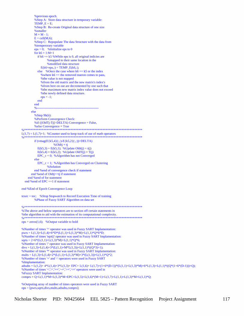
Nicholas Shorter PID: N0425664 EEL 5825 – Pattern Recognition Project Assignment 117
%previous epoch. %Step A: Store data structure in temporary variable: TEMP_E = E; %Step B: Re-create Original data structure of one size %smaller M = M - 1; E = cell(M,6); %Step C: Repopulate The data Structure with the data from %temperorary variable eps = 0; %Initialize eps to 0 for k6 = 1:M+1 if k6 ~= k5 %While eps is 0, all original indicies are %mapped to their same location in the %modified data structure E(k6+eps,:) = TEMP_E(k6,:); else %Once the case where k6 == k5 or the index %where k6 == the removed nueron comes to pass, %the value is not mapped %from the old matrix and the new matrix's index's %from here on out are decremented by one such that %the maximum new matrix index value does not exceed %the newly defined data structure. eps = -1; end end %---------------------------------------------------------- else %Step 9b(ii): %Perform Convergence Check: %if (||OldTj-Tj||>DELTA) Convergence = False, %else Convergence = True %************************************************************************** L(1,7) = L(1,7)+1; %Counter used to keep track of use of math operators %************************************************************************** if (vmag(E{k5,4}(:,:)-E{k5,2}(:,:))>DELTA) %Oldtj = tj E(k5,3) = E(k5,1); %Update Oldt(j) = t(j) E(k5,4) = E(k5,2); %Update OldT(j) = T(j) EPC_c = 0; %Algorithm has not Converged else EPC_c = 1; %Algorithm has Converged on Clustering %Solution end %end of convergence check if statement end %end of Oldtj==tj if statement end %end of for statement end %end of EPC ==1 if statement end %End of Epoch Convergence Loop texec = toc; %Stop Stopwatch to Record Execution Time of training %Phase of Fuzzy SART Algorithm on data set %************************************************************************** %The above and below seperators are to section off certain statements in %the algorithm to aid with the estimation of its computational complexity. %************************************************************************** ops = zeros(1,6); %Output variable to hold %Number of times '^' operator was used in Fuzzy SART Implamentation: pwrs = L(1,3)+L(1,4)+6*D*(L(1,1)+L(1,3)*M)+L(1,1)*Q*6*D; %Number of times 'sqrt()' operator was used in Fuzzy SART Implamentation: sqrts = 2+6*(L(1,1)+L(1,3)*M)+L(1,1)*Q*6; %Number of times '/' operator was used in Fuzzy SART Implamentation: divs = L(1,3)+L(1,4)+3*(L(1,1)+M*L(1,3))+L(1,1)*((Q*3)+1); %Number of times '*' operator was used in Fuzzy SART Implamentation: mults = L(1,3)+L(1,4)+2*(L(1,1)+L(1,3)*M)+3*(L(1,3))+L(1,1)*Q*2; %Number of times '+' and '-' operators were used in Fuzzy SART %Implamentation: adsubs = L(1,2)+ 4*L(1,4)+3*L(1,3)+ EPC+ L(1,6)+ L(1,7)+(1+6*(D-1))*(L(1,1)+L(1,3)*M)+6*L(1,3)+L(1,1)*((Q*(1+6*(D-1)))+Q); %Number of times '<','>','==','~=','>=','<=' operators were used in %Fuzzy SART Implamentation: comprs = Q+L(1,1)*M+L(1,3)*M+EPC+L(1,5)+L(1,6)*(M+1)+L(1,7)+L(1,1)+L(1,3)*M+L(1,1)*Q; %Outputing array of number of times operators were used in Fuzzy SART ops = [pwrs,sqrts,divs,mults,adsubs,comprs];
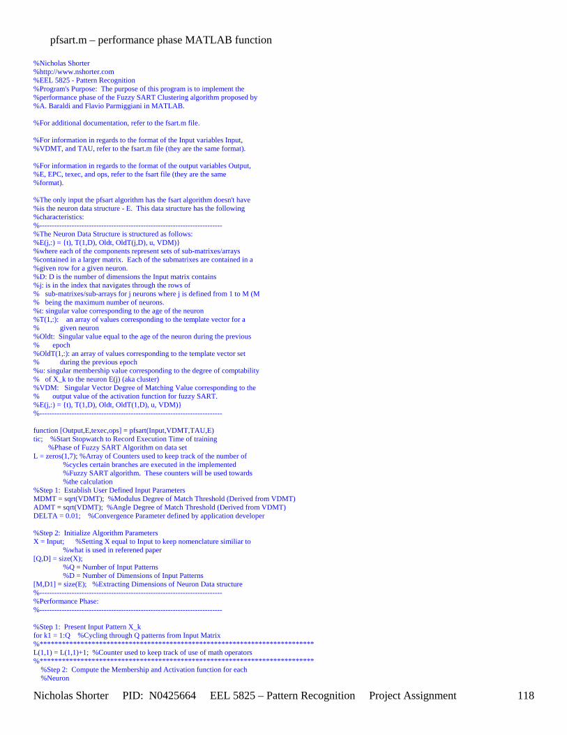
Nicholas Shorter PID: N0425664 EEL 5825 – Pattern Recognition Project Assignment 118
pfsart.m – performance phase MATLAB function %Nicholas Shorter %http://www.nshorter.com %EEL 5825 - Pattern Recognition %Program's Purpose: The purpose of this program is to implement the %performance phase of the Fuzzy SART Clustering algorithm proposed by %A. Baraldi and Flavio Parmiggiani in MATLAB. %For additional documentation, refer to the fsart.m file. %For information in regards to the format of the Input variables Input, %VDMT, and TAU, refer to the fsart.m file (they are the same format). %For information in regards to the format of the output variables Output, %E, EPC, texec, and ops, refer to the fsart file (they are the same %format). %The only input the pfsart algorithm has the fsart algorithm doesn't have %is the neuron data structure - E. This data structure has the following %characteristics: %-------------------------------------------------------------------------- %The Neuron Data Structure is structured as follows: %E(j,:) = {t), T(1,D), Oldt, OldT(j,D), u, VDM)} %where each of the components represent sets of sub-matrixes/arrays %contained in a larger matrix. Each of the submatrixes are contained in a %given row for a given neuron. %D: D is the number of dimensions the Input matrix contains %j: is in the index that navigates through the rows of % sub-matrixes/sub-arrays for j neurons where j is defined from 1 to M (M % being the maximum number of neurons. %t: singular value corresponding to the age of the neuron %T(1,:): an array of values corresponding to the template vector for a % given neuron %Oldt: Singular value equal to the age of the neuron during the previous % epoch %OldT(1,:): an array of values corresponding to the template vector set % during the previous epoch %u: singular membership value corresponding to the degree of comptability % of X_k to the neuron E(j) (aka cluster) %VDM: Singular Vector Degree of Matching Value corresponding to the % output value of the activation function for fuzzy SART. %E(j,:) = {t), T(1,D), Oldt, OldT(1,D), u, VDM)} %-------------------------------------------------------------------------- function [Output,E,texec,ops] = pfsart(Input,VDMT,TAU,E) tic; %Start Stopwatch to Record Execution Time of training %Phase of Fuzzy SART Algorithm on data set L = zeros(1,7); %Array of Counters used to keep track of the number of %cycles certain branches are executed in the implemented %Fuzzy SART algorithm. These counters will be used towards %the calculation %Step 1: Establish User Defined Input Parameters MDMT = sqrt(VDMT); %Modulus Degree of Match Threshold (Derived from VDMT) ADMT = sqrt(VDMT); %Angle Degree of Match Threshold (Derived from VDMT) DELTA = 0.01; %Convergence Parameter defined by application developer %Step 2: Initialize Algorithm Parameters X = Input; %Setting X equal to Input to keep nomenclature similiar to %what is used in referened paper [Q,D] = size(X); %Q = Number of Input Patterns %D = Number of Dimensions of Input Patterns [M,D1] = size(E); %Extracting Dimensions of Neuron Data structure %-------------------------------------------------------------------------- %Performance Phase: %-------------------------------------------------------------------------- %Step 1: Present Input Pattern X_k for k1 = 1:Q %Cycling through Q patterns from Input Matrix %************************************************************************** L(1,1) = L(1,1)+1; %Counter used to keep track of use of math operators %************************************************************************** %Step 2: Compute the Membership and Activation function for each %Neuron
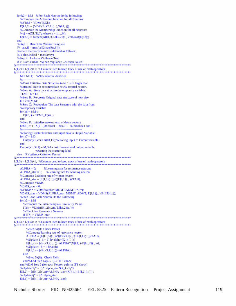
Nicholas Shorter PID: N0425664 EEL 5825 – Pattern Recognition Project Assignment 119
for k2 = 1:M %For Each Neuron do the following: %Compute the Activation function for all Neurons: %VDM = VDM(Tj,Xk); E(k2,6) = {VDM(E{k2,2}(:,:),X(k1,:))}; %Compute the Membership Function for all Neurons: %uj = u(Xk,Tj,Tp where p = 1,...,M); E(k2,5) = {umem(X(k1,:),E{k2,2}(:,:),cell2mat(E(:,2)))}; end %Step 3: Detect the Winner Template [V_star,I] = max(cell2mat(E(:,6))); %where the function max is defined as follows: %[Value,Index] = max(array) %Step 4: Perform Vigilance Test if V_star<VDMT %Then Vigilance Criterion Failed %************************************************************************** L(1,2) = L(1,2)+1; %Counter used to keep track of use of math operators %************************************************************************** M = M+1; %New neuron identifier %---------------------------------------------------------- %Must Initialize Data Structure to be 1 size larger than %original size to accommodate newly created neuron. %Step A: Store data structure in temporary variable: TEMP_E = E; %Step B: Re-create Original data structure of new size E = cell(M,6); %Step C: Repopulate The data Structure with the data from %temporary variable for k6 = 1:M-1 E(k6,:) = TEMP_E(k6,:); end %Step D: Initialize newest term of data structure E(M,:) = {1,X(k1,:),0,zeros(1,D),0,0}; %Initialize t and T %---------------------------------------------------------- %Storing Cluster Number and Input data to Output Variable: for k7 = 1:D Output(k1,k7) = X(k1,k7);%Storing Input to Output variable end Output(k1,D+1) = M;%As last dimension of output variable, %writing the clustering label else %Vigilance Criterion Passed %************************************************************************** L(1,3) = L(1,3)+1; %Counter used to keep track of use of math operators %************************************************************************** ALPHA = 0; %Learning rate for resonance neurons ALPHA_star = 0; %Learning rate for winning neuron %Compute Learning rate of winner neuron ALPHA_star = (E{I,6}(:,:))^((E{I,1}(:,:))/TAU); %Compute VDMS VDMS_star = 0; %VDMS* = VDMS(alpha*,MDMT,ADMT,t*,u*); VDMS_star = VDMS(ALPHA_star, MDMT, ADMT, E{I,1}(:,:),E{I,5}(:,:)); %Step 5 for Each Neuron Do the Following for k3 = 1:M %Compute the Inter-Template Similarity Value ITSj = VDM((E{I,2}(:,:)),(E{k3,2}(:,:))); %Check for Resonance Neurons if ITSj > VDMS_star %************************************************************************** L(1,4) = L(1,4)+1; %Counter used to keep track of use of math operators %************************************************************************** %Step 5a(i): Check Passes %Compute learning rate of resonance neuron ALPHA = (E{k3,5}(:,:))^((E{k3,1}(:,:)+E{I,1}(:,:))/TAU); %Update T_h = T_h+alpha*(X_k-T_h) E(k3,2) = {(E{k3,2}(:,:))+ALPHA*(X(k1,:)-E{k3,2}(:,:))}; %Update t_h = t_h+alpha E(k3,1) = {(E{k3,1}(:,:))+ALPHA}; else %Step 5a(ii): Check Fails end %End Step 6a(i & ii) -> ITS check end %End Step 5 (for each Neuron peform ITS check) %Update Tj* = Tj*+alpha_star*(X_k=Tj*) E(I,2) = {(E{I,2}(:,:))+ALPHA_star*(X(k1,:)-E{I,2}(:,:))}; %Update tj* = tj*+alpha_star E(I,1) = {(E{I,1}(:,:))+ALPHA_star};
Nicholas Shorter PID: N0425664 EEL 5825 – Pattern Recognition Project Assignment 120
%Storing Cluster Number and Input data to Output Variable: for k7 = 1:D Output(k1,k7) = X(k1,k7);%Storing Input to Output variable end Output(k1,D+1) = I; %last dimension of output variable, %writing the clustering label end %End of Step 4 (vigilance test) end %End of Step 1 (Present Input Pattern) texec = toc; %Stop Stopwatch to Record Execution Time of training %Phase of Fuzzy SART Algorithm on data set %************************************************************************** %The above and below separators are to section off certain statements in %the algorithm to aid with the estimation of its computational complexity. %************************************************************************** ops = zeros(1,6); %Output variable to hold %Number of times '^' operator was used in Fuzzy SART Implementation: pwrs = L(1,3)+L(1,4)+6*D*(L(1,1)+L(1,3)*M)+L(1,1)*Q*6*D; %Number of times 'sqrt()' operator was used in Fuzzy SART Implementation: sqrts = 2+6*(L(1,1)+L(1,3)*M)+L(1,1)*Q*6; %Number of times '/' operator was used in Fuzzy SART Implementation: divs = L(1,3)+L(1,4)+3*(L(1,1)+M*L(1,3))+L(1,1)*((Q*3)+1); %Number of times '*' operator was used in Fuzzy SART Implementation: mults = L(1,3)+L(1,4)+2*(L(1,1)+L(1,3)*M)+3*(L(1,3))+L(1,1)*Q*2; %Number of times '+' and '-' operators were used in Fuzzy SART %Implementation: adsubs = L(1,2)+ 4*L(1,4)+3*L(1,3)+(1+6*(D-1))*(L(1,1)+L(1,3)*M)+6*L(1,3)+L(1,1)*((Q*(1+6*(D-1)))+Q); %Number of times '<','>','==','~=','>=','<=' operators were used in %Fuzzy SART Implementation: comprs = Q+L(1,1)*M+L(1,3)*M+L(1,1)+L(1,3)*M+L(1,1)*Q; %Outputing array of number of times operators were used in Fuzzy SART ops = [pwrs,sqrts,divs,mults,adsubs,comprs];

Nicholas Shorter PID: N0425664 EEL 5825 – Pattern Recognition Project Assignment 121
8 Appendix 8 – Reference List for Survey of Clustering Algorithms Reference List for Survey of Clustering Algorithms :
1. S. Guha, R. Rastogi, and K. Shim, “CURE: An efficient clustering algorithm for large databases,” in Proc. ACM SIGMOD Int. Conf. Management of Data, 1998, pp. 73–84.
2. S. Guha, R. Rastogi, and K. Shim, “ROCK: A robust clustering algorithm for categorical attributes,” Inf. Syst., vol. 25, no. 5, pp. 345–366, 2000. 3. G. Karypis, E. Han, and V. Kumar, “Chameleon: Hierarchical clustering using dynamic modeling,” IEEE Computer, vol. 32, no. 8, pp. 68–75, Aug. 1999. 4. T. Zhang, R. Ramakrishnan, and M. Livny, “BIRCH: An efficient data clustering method for very large databases,” in Proc. ACM SIGMOD Conf.
Management of Data, 1996, pp. 103–114. 5. E. Forgy, “Cluster analysis of multivariate data: Efficiency vs. interpretability of classifications,” Biometrics, vol. 21, pp. 768–780, 1965. 6. J. MacQueen, “Some methods for classification and analysis of multivariate observations,” in Proc. 5th Berkeley Symp., vol. 1, 1967, pp. 281–297. 7. G. Ball and D. Hall, “A clustering technique for summarizing multivariate data,” Behav. Sci., vol. 12, pp. 153–155, 1967. 8. G. Patanè and M. Russo, “The enhanced-LBG algorithm,” Neural Netw., vol. 14, no. 9, pp. 1219–1237, 2001. 9. K. Krishna and M. Murty, “Genetic K-means algorithm,” IEEE Trans. Syst., Man, Cybern. B, Cybern., vol. 29, no. 3, pp. 433–439, Jun. 1999. 10. L. Kaufman and P. Rousseeuw, Finding Groups in Data: An Introduction to Cluster Analysis: Wiley, 1990. 11. G. McLachlan and T. Krishnan, The EM Algorithm and Extensions. New York: Wiley, 1997. 12. F. Harary, Graph Theory. Reading, MA: Addison-Wesley, 1969. 13. L. Zadeh, “Fuzzy sets,” Inf. Control, vol. 8, pp. 338–353, 1965. 14. J. Williamson, “Gaussian ARTMAP: A neural network for fast incremental learning of noisy multidimensional maps,” Neural Netw., vol. 9, no. 5, pp. 881–
897, 1996. 15. G. Anagnostopoulos and M. Georgiopoulos, “Hypersphere ART and ARTMAP for unsupervised and supervised incremental learning,” in Proc. IEEE-INNS-
ENNS Int. Joint Conf. Neural Networks (IJCNN’00), vol. 6, Como, Italy, pp. 59–64. 16. Y. Zhang and Z. Liu, “Self-splitting competitive learning: A new on-line clustering paradigm,” IEEE Trans. Neural Networks, vol. 13, no. 2, pp. 369–380,
Mar. 2002. 17. G. Milligan and M. Cooper, “An examination of procedures for determining the number of clusters in a data set,” Psychometrika, vol. 50, pp. 159–179,
1985. 18. UCI Machine Learning Repository http://www.ics.uci.edu/~mlearn/MLRepository.html 19. R. Sharan and R. Shamir, “CLICK: A clustering algorithm with applications to gene expression analysis,” in Proc. 8th Int. Conf. Intelligent Systems for
Molecular Biology, 2000, pp. 307–316. 20. Carpenter, G.A., Grossberg, S., & Reynolds, J.H. , ARTMAP: Supervised real-time learning and classification of nonstationary data by a self-organizing
neural network. Neural Networks, 4, 565-588. (1991). 21. Carpenter, G.A. & Grossberg, S. “Adaptive Resonance Theory.” In M.A. Arbib (Ed.), The Handbook of Brain Theory and Neural Networks, Second
Edition, Cambridge, (2003). 22. Carpenter, G.A. & Grossberg, S. “A massively parallel architecture for a self-organizing neural pattern recognition machine.” Computer Vision, Graphics,
and Image Processing, 37, 54-115. (1987). 23. Carpenter, G.A., Grossberg, S., & Rosen, D.B. “ART 2-A: An adaptive resonance algorithm for rapid category learning and recognition.” Neural Networks,
4, 493-504. (1991). 24. Carpenter, G.A. & Grossberg, S. “ART 3: Hierarchical search using chemical transmitters in self- organizing pattern recognition architectures.” Neural
Networks, 3, 129-152. (1990).
Nicholas Shorter PID: N0425664 EEL 5825 – Pattern Recognition Project Assignment 122
9 Appendix 9 – Reference List for Project 3 References:
25. A. K. Jain, M.N. Murty, and P.J. Flynn, “Data Clustering: A Review”, ACM Computing Surveys, Vol. 31, No. 3, September 1999. 26. Baraldi, A.; Alpaydin, E.; “Constructive feedforward ART clustering networks. I”, Neural Networks, IEEE Transactions on, Volume 13,
Issue 3, May 2002 pp. 645 – 661 27. Baraldi, A.; Alpaydin, E.; “Constructive feedforward ART clustering networks. II”, Neural Networks, IEEE Transactions on, Volume 13,
Issue 3, May 2002 pp.662 – 677 28. Baraldi, A.; Blonda, P.; “A survey of fuzzy clustering algorithms for pattern recognition. I”, Systems, Man and Cybernetics, Part B, IEEE
Transactions on, Volume 29, Issue 6, Dec. 1999 Page(s):778 - 785 29. Baraldi, A.; Blonda, P.; “A survey of fuzzy clustering algorithms for pattern recognition. II”, Systems, Man and Cybernetics, Part B, IEEE
Transactions on, Volume 29, Issue 6, Dec. 1999 Page(s):786 - 801 30. Baraldi, A.; Parmiggani, F.; “A self-organizing neural network merging Kohonen’s and ART models”, Proceedings., IEEE International
Conference on, Volume 5, 27 Nov.-1 Dec. 1995 pp. 2444 - 2449 vol.5 31. Baraldi, A.; Parmiggiani, F.; “Fuzzy combination of Kohonen's and ART neural network models to detect statistical regularities in a
random sequence of multi-valued input patterns”, Neural Networks,1997., International Conference on, Volume 1, 9-12 June 1997 pp.281 - 286 vol.1
32. Carpenter, G.A.; Grossberg, S.; “A massively parallel architecture for a self-organizing neural pattern recognition machine”, Computer Vision, Graphics, and Image Processing, 37, 1987, pp. 54-115
33. Carpenter, G.A.; Grossberg, S.; Rosen, D.B.; “Fuzzy ART: Fast stable learning and categorization of analog patterns by an adaptive resonance system”, Neural Networks, 4, 1991, pp.759-771
34. R. Xu, D. Wunch, II, “Survey of Clustering Algorithms”, IEEE Transactions on Neural Networks, Vol. 16, No. 3, May 2005, pp. 645-678. 35. CELEST Technology Website - http://profusion.bu.edu/techlab/modules/mydownloads/viewcat.php?cid=26&pid=2&sub=1 36. Kangas, J.A.; Kohonen, T.; Laaksonen, J.T.; “Variants of self organizing maps.” IEEE Trans. Neural Networks, vol. 1, pp. 93-99, 1990. 37. Baraldi, A.; and Parmiggiani, F.; “A neural network model for unsupervised categorization of multivalued input patterns: an application to
satellite image clustering,” IEEE Trans. Geosci. Remote Sensing, vol 33, no. 2, pp. 305-316, March 1995. 38. Kohonen, T.; “The self-organizing map”, Proceedings of the IEEE, vol 78, nol 9, pp. 1464-1480, Sept. 1990 39. Implementation of LAPACK http://www.mathworks.com/company/newsletters/news_notes/clevescorner/winter2000.cleve.html 40. PAPI package (flops work around) for MATLAB -
http://www.mathworks.com/matlabcentral/fileexchange/loadFile.do?objectId=5445&objectType=File 41. The Lightspeed MATLAB toolbox (flops workaround) for MATLAB - http://research.microsoft.com/~minka/software/lightspeed/ 42. J. A. Benediktsson, P.H. Swain, and O. K. Ersoy, “Neural network approaches versus statistical methods in classification of multisource
remote sensing data,” IEEE Trans. Geosci. Remote Sensing, vol. 28, pp. 540 – 551, July 1990. 43. J.A. Kangas, T. Kohonen and J. T. Laaksonen, “Variants of self-organizing maps,” IEE Trans. Neural Networks, vol .1 pp. 93-99, 1990. 44. Bezdeck, J.C.; and Pal, N. R.; “Two soft relatives of learning vector quantization.” Neural Networks, vol 8, pp. 729-743, 1995.