Noise2Self: Blind Denoising by Self-Supervision

Joshua Batson * 1 Loic Royer * 1

AbstractWe propose a general framework for denoisinghigh-dimensional measurements which requiresno prior on the signal, no estimate of the noise,and no clean training data. The only assumptionis that the noise exhibits statistical independenceacross different dimensions of the measurement,while the true signal exhibits some correlation.For a broad class of functions (“J -invariant”), itis then possible to estimate the performance ofa denoiser from noisy data alone. This allowsus to calibrate J -invariant versions of any pa-rameterised denoising algorithm, from the singlehyperparameter of a median filter to the millionsof weights of a deep neural network. We demon-strate this on natural image and microscopy data,where we exploit noise independence betweenpixels, and on single-cell gene expression data,where we exploit independence between detec-tions of individual molecules. This frameworkgeneralizes recent work on training neural netsfrom noisy images and on cross-validation formatrix factorization.

1. IntroductionWe would often like to reconstruct a signal from high-dimensional measurements that are corrupted, under-sampled, or otherwise noisy. Devices like high-resolutioncameras, electron microscopes, and DNA sequencers arecapable of producing measurements in the thousands to mil-lions of feature dimensions. But when these devices arepushed to their limits, taking videos with ultra-fast framerates at very low-illumination, probing individual moleculeswith electron microscopes, or sequencing tens of thousandsof cells simultaneously, each individual feature can becomequite noisy. Nevertheless, the objects being studied are of-ten very structured and the values of different features are

*Equal contribution 1Chan-Zuckerberg Biohub. Correspon-dence to: Joshua Batson <joshua.batson@czbiohub.org>, LoicRoyer <loic.royer@czbiohub.org>.

Proceedings of the 36 th International Conference on MachineLearning, Long Beach, California, PMLR 97, 2019. Copyright2019 by the author(s).

highly correlated. Speaking loosely, if the “latent dimen-sion” of the space of objects under study is much lower thanthe dimension of the measurement, it may be possible toimplicitly learn that structure, denoise the measurements,and recover the signal without any prior knowledge of thesignal or the noise.

Traditional denoising methods each exploit a property ofthe noise, such as Gaussianity, or structure in the signal,such as spatiotemporal smoothness, self-similarity, or hav-ing low-rank. The performance of these methods is limitedby the accuracy of their assumptions. For example, if thedata are genuinely not low rank, then a low rank modelwill fit it poorly. This requires prior knowledge of the sig-nal structure, which limits application to new domains andmodalities. These methods also require calibration, as hy-perparameters such as the degree of smoothness, the scale ofself-similarity, or the rank of a matrix have dramatic impactson performance.

In contrast, a data-driven prior, such as pairs (xi, yi) ofnoisy and clean measurements of the same target, can beused to set up a supervised learning problem. A neuralnet trained to predict yi from xi may be used to denoisenew noisy measurements (Weigert et al., 2018). As longas the new data are drawn from the same distribution, onecan expect performance similar to that observed duringtraining. Lehtinen et al. demonstrated that clean targets areunnecessary (2018). A neural net trained on pairs (xi, x′i)of independent noisy measurements of the same target will,under certain distributional assumptions, learn to predict theclean signal. These supervised approaches extend to imagedenoising the success of convolutional neural nets, whichcurrently give state-of-the-art performance for a vast rangeof image-to-image tasks. Both of these methods require anexperimental setup in which each target may be measuredmultiple times, which can be difficult in practice.

In this paper, we propose a framework for blind denoisingbased on self-supervision. We use groups of features whosenoise is independent conditional on the true signal to predictone another. This allows us to learn denoising functionsfrom single noisy measurements of each object, with per-formance close to that of supervised methods. The sameapproach can also be used to calibrate traditional image de-noising methods such as median filters and non-local means,

Noise2Self: Blind Denoising by Self-Supervision

independent feature dimensions

a

independent images

b

independent pixels

cACTG...TGAC

TTAG...GAGC

CGCA...ACAC

ACCT...TGAG

ACCT...GGTT

ACCG...TGTA

ACCT...GATC

CGCT...GTGT

ATAT...CGTC

ACCT...TGAC

GCGT...CGAC

TAGC...CTCA

ACAT...GAGG

TTCG...AGAT

independent molecules

d

Figure 1. (a) The box represents the dimensions of the measurement x. J is a subset of the dimensions, and f is a J-invariant function: ithas the property that the value of f(x) restricted to dimensions in J , f(x)J , does not depend on the value of x restricted to J , xJ . Thisenables self-supervision when the noise in the data is conditionally independent between sets of dimensions. Here are 3 examples ofdimension partitioning: (b) two independent image acquisitions, (c) independent pixels of a single image, (d) independently detected RNAmolecules from a single cell.

and, using a different independence structure, denoise highlyunder-sampled single-cell gene expression data.

We model the signal y and its noisy measurement x as a pairof random variables in Rm. If J ⊂ {1, . . . ,m} is a subsetof the dimensions, we write xJ for x restricted to J .

Definition. Let J be a partition of the dimensions{1, . . . ,m} and let J ∈ J . A function f : Rm → Rmis J-invariant if f(x)J does not depend on the value of xJ .It is J -invariant if it is J-invariant for each J ∈ J .

We propose minimizing the self-supervised loss

L(f) = E ‖f(x)− x‖2 , (1)

overJ -invariant functions f . Since f has to use informationfrom outside of each subset of dimensions J to predict thevalues inside of J , it cannot merely be the identity.

Proposition 1. Suppose x is an unbiased estimator of y, i.e.E[x|y] = y, and the noise in each subset J ∈ J is indepen-dent from the noise in its complement Jc, conditional on y.Let f be J -invariant. Then

E ‖f(x)− x‖2 = E ‖f(x)− y‖2 + E ‖x− y‖2 . (2)

That is, the self-supervised loss is the sum of the ordinarysupervised loss and the variance of the noise. By minimizingthe self-supervised loss over a class ofJ -invariant functions,one may find the optimal denoiser for a given dataset.

For example, if the signal is an image with independent,mean-zero noise in each pixel, we may choose J ={{1}, . . . , {m}} to be the singletons of each coordinate.Then “donut” median filters, with a hole in the center, forma class of J -invariant functions, and by comparing the valueof the self-supervised loss at different filter radii, we areable to select the optimal radius for denoising the image athand (See §3).

The donut median filter has just one parameter and thereforelimited ability to adapt to the data. At the other extreme,

we may search over all J -invariant functions for the globaloptimum:Proposition 2. The J -invariant function f∗J minimizing (1)satisfies

f∗J (x)J = E[yJ |xJc ]

for each subset J ∈ J .

That is, the optimal J -invariant predictor for the dimensionsof y in some J ∈ J is their expected value conditional onobserving the dimensions of x outside of J .

In §4, we use analytical examples to illustrate how the opti-mal J -invariant denoising function approaches the optimalgeneral denoising function as the amount of correlationbetween features in the data increases.

In practice, we may attempt to approximate the optimaldenoiser by searching over a very large class of functions,such as deep neural networks with millions of parameters. In§5, we show that a deep convolutional network, modified tobecome J -invariant using a masking procedure, can achievestate-of-the-art blind denoising performance on three diversedatasets.

Sample code is available on GitHub1 and deferred proofsare contained in the Supplement.

2. Related WorkEach approach to blind denoising relies on assumptionsabout the structure of the signal and/or the noise. We re-view the major categories of assumption below, and thetraditional and modern methods that utilize them. Most ofthe methods below are described in terms of application toimage denoising, which has the richest literature, but somehave natural extensions to other spatiotemporal signals andto generic measurements of vectors.

Smoothness: Natural images and other spatiotemporal sig-nals are often assumed to vary smoothly (Buades et al.,

1https://github.com/czbiohub/noise2self

Noise2Self: Blind Denoising by Self-Supervision

2005b). Local averaging, using a Gaussian, median, orsome other filter, is a simple way to smooth out a noisyinput. The degree of smoothing to use, e.g., the width of afilter, is a hyperparameter often tuned by visual inspection.

Self-Similarity: Natural images are often self-similar, inthat each patch in an image is similar to many other patchesfrom the same image. The classic non-local means algo-rithm replaces the center pixel of each patch with a weightedaverage of central pixels from similar patches (Buades et al.,2005a). The more robust BM3D algorithm makes stacksof similar patches, and performs thresholding in frequencyspace (Dabov et al., 2007). The hyperparameters of thesemethods have a large effect on performance (Lebrun, 2012),and on a new dataset with an unknown noise distribution itis difficult to evaluate their effects in a principled way.

Convolutional neural nets can produce images with anotherform of self-similarity, as linear combinations of the samesmall filters are used to produce each output. The “deepimage prior” of (Ulyanov et al., 2017) exploits this by train-ing a generative CNN to produce a single output image andstopping training before the net fits the noise.

Generative: Given a differentiable, generative model ofthe data, e.g. a neural net G trained using a generativeadversarial loss, data can be denoised through projectiononto the range of the net (Tripathi et al., 2018).

Gaussianity: Recent work (Zhussip et al., 2018; Metzleret al., 2018) uses a loss based on Stein’s unbiased risk esti-mator to train denoising neural nets in the special case thatnoise is i.i.d. Gaussian.

Sparsity: Natural images are often close to sparse in e.g. awavelet or DCT basis (Chang et al., 2000). Compressionalgorithms such as JPEG exploit this feature by thresholdingsmall transform coefficients (Pennebaker & Mitchell, 1992).This is also a denoising strategy, but artifacts familiar frompoor compression (like the ringing around sharp edges)may occur. Hyperparameters include the choice of basisand the degree of thresholding. Other methods learn anovercomplete dictionary from the data and seek sparsity inthat basis (Elad & Aharon, 2006; Papyan et al., 2017).

Compressibility: A generic approach to denoising is tolossily compress and then decompress the data. The accu-racy of this approach depends on the applicability of thecompression scheme used to the signal at hand and its ro-bustness to the form of noise. It also depends on choosingthe degree of compression correctly: too much will loseimportant features of the signal, too little will preserve allof the noise. For the sparsity methods, this “knob” is thedegree of sparsity, while for low-rank matrix factorizations,it is the rank of the matrix.

Autoencoder architectures for neural nets provide a gen-

eral framework for learnable compression. Each sampleis mapped to a low-dimensional representation—the valueof the neural net at the bottleneck layer— then back to theoriginal space (Gallinari et al., 1987; Vincent et al., 2010).An autoencoder trained on noisy data may produce cleanerdata as its output. The degree of compression is determinedby the width of the bottleneck layer.

UNet architectures, in which skip connections are added toa typical autoencoder architecture, can capture high-levelspatially coarse representations and also reproduce finedetail; they can, in particular, learn the identity function(Ronneberger et al., 2015). Trained directly on noisy data,they will do no denoising. Trained with clean targets, theycan learn very accurate denoising functions (Weigert et al.,2018).

Statistical Independence: Lehtinen et al. observed that aUNet trained to predict one noisy measurement of a signalfrom an independent noisy measurement of the same signalwill in fact learn to predict the true signal (Lehtinen et al.,2018). We may reformulate the Noise2Noise procedurein terms of J -invariant functions: if x1 = y + n1 andx2 = y + n2 are the two measurements, we consider thecomposite measurement x = (x1, x2) of a composite signal(y, y) in R2m and set J = {J1, J2} = {{1, . . . ,m}, {m+1, . . . , 2m}}. Then f∗J (x)J2 = E[y|x1].

An extension to video, in which one frame is used to com-pute the pullback under optical flow of another, was ex-plored in (Ehret et al., 2018).

In concurrent work, Krull et al. train a UNet to predict a col-lection of held-out pixels of an image from a version of thatimage with those pixels replaced (2018). A key differencebetween their approach and our neural net examples in §5is in that their replacement strategy is not quite J -invariant.(With some probability a given pixel is replaced by itself.)While their method lacks a theoretical guarantee againstfitting the noise, it performs well in practice, on natural andmicroscopy images with synthetic and real noise.

Finally, we note that the “fully emphasized denoising au-toencoders” in (Vincent et al., 2010) used the MSE betweenan autoencoder evaluated on masked input data and the truevalue of the masked pixels, but with the goal of learningrobust representations, not denoising.

3. Calibrating Traditional ModelsMany denoising models have a hyperparameter controllingthe degree of the denoising—the size of a filter, the thresh-old for sparsity, the number of principal components. Ifground truth data were available, the optimal parameter θfor a family of denoisers fθ could be chosen by minimizing‖fθ(x)− y‖2. Without ground truth, we may nevertheless

Noise2Self: Blind Denoising by Self-Supervision

r=1 r=2 r=3 r=4 r=5 r=6

noisynoisy

ground truthground truth

ground truth

self-supervised

donutclassic

donutclassic

Mean

sq

uare

err

or

(MS

E)

Radius of median filter

donut classic

r

more blurrymore noisy

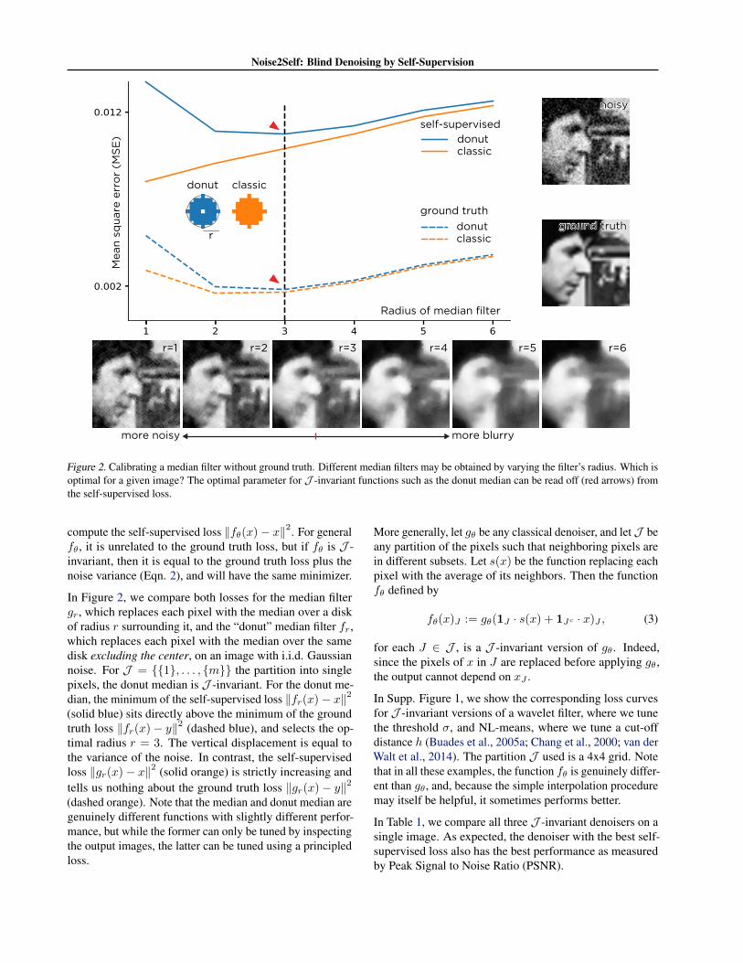
Figure 2. Calibrating a median filter without ground truth. Different median filters may be obtained by varying the filter’s radius. Which isoptimal for a given image? The optimal parameter for J -invariant functions such as the donut median can be read off (red arrows) fromthe self-supervised loss.

compute the self-supervised loss ‖fθ(x)− x‖2. For generalfθ, it is unrelated to the ground truth loss, but if fθ is J -invariant, then it is equal to the ground truth loss plus thenoise variance (Eqn. 2), and will have the same minimizer.

In Figure 2, we compare both losses for the median filtergr, which replaces each pixel with the median over a diskof radius r surrounding it, and the “donut” median filter fr,which replaces each pixel with the median over the samedisk excluding the center, on an image with i.i.d. Gaussiannoise. For J = {{1}, . . . , {m}} the partition into singlepixels, the donut median is J -invariant. For the donut me-dian, the minimum of the self-supervised loss ‖fr(x)− x‖2(solid blue) sits directly above the minimum of the groundtruth loss ‖fr(x)− y‖2 (dashed blue), and selects the op-timal radius r = 3. The vertical displacement is equal tothe variance of the noise. In contrast, the self-supervisedloss ‖gr(x)− x‖2 (solid orange) is strictly increasing andtells us nothing about the ground truth loss ‖gr(x)− y‖2(dashed orange). Note that the median and donut median aregenuinely different functions with slightly different perfor-mance, but while the former can only be tuned by inspectingthe output images, the latter can be tuned using a principledloss.

More generally, let gθ be any classical denoiser, and let J beany partition of the pixels such that neighboring pixels arein different subsets. Let s(x) be the function replacing eachpixel with the average of its neighbors. Then the functionfθ defined by

fθ(x)J := gθ(1J · s(x) + 1Jc · x)J , (3)

for each J ∈ J , is a J -invariant version of gθ. Indeed,since the pixels of x in J are replaced before applying gθ,the output cannot depend on xJ .

In Supp. Figure 1, we show the corresponding loss curvesfor J -invariant versions of a wavelet filter, where we tunethe threshold σ, and NL-means, where we tune a cut-offdistance h (Buades et al., 2005a; Chang et al., 2000; van derWalt et al., 2014). The partition J used is a 4x4 grid. Notethat in all these examples, the function fθ is genuinely differ-ent than gθ, and, because the simple interpolation proceduremay itself be helpful, it sometimes performs better.

In Table 1, we compare all three J -invariant denoisers on asingle image. As expected, the denoiser with the best self-supervised loss also has the best performance as measuredby Peak Signal to Noise Ratio (PSNR).

Noise2Self: Blind Denoising by Self-Supervision

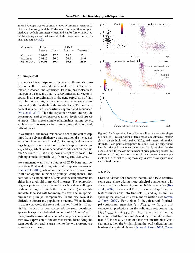
Table 1. Comparison of optimally tuned J -invariant versions ofclassical denoising models. Performance is better than originalmethod at default parameter values, and can be further improved(+) by adding an optimal amount of the noisy input to the J -invariant output (§4.2).

METHOD LOSS PSNRJ-INVT J-INVT J-INVT+ DEFAULT

MEDIAN 0.0107 27.5 28.2 27.1WAVELET 0.0113 26.0 26.9 24.6NL-MEANS 0.0098 30.4 30.8 28.9

3.1. Single-Cell

In single-cell transcriptomic experiments, thousands of in-dividual cells are isolated, lysed, and their mRNA are ex-tracted, barcoded, and sequenced. Each mRNA molecule ismapped to a gene, and that ∼20,000-dimensional vector ofcounts is an approximation to the gene expression of thatcell. In modern, highly parallel experiments, only a fewthousand of the hundreds of thousands of mRNA moleculespresent in a cell are successfully captured and sequenced(Milo et al., 2010). Thus the expression vectors are very un-dersampled, and genes expressed at low levels will appearas zeros. This makes simple relationships among genes,such as co-expression or transitions during development,difficult to see.

If we think of the measurement as a set of molecules cap-tured from a given cell, then we may partition the moleculesat random into two sets J1 and J2. Summing (and normaliz-ing) the gene counts in each set produces expression vectorsxJ1 and xJ2 which are independent conditional on the truemRNA content y. We may now attempt to denoise x bytraining a model to predict xJ2 from xJ1 and vice versa.

We demonstrate this on a dataset of 2730 bone marrowcells from Paul et al. using principal component regression(Paul et al., 2015), where we use the self-supervised lossto find an optimal number of principal components. Thedata contain a population of stem cells which differentiateeither into erythroid or myeloid lineages. The expressionof genes preferentially expressed in each of these cell typesis shown in Figure 3 for both the (normalized) noisy dataand data denoised with too many, too few, and an optimalnumber of principal components. In the raw data, it isdifficult to discern any population structure. When the datais under-corrected, the stem cell marker Ifitm1 is still notvisible. When it is over-corrected, the stem populationappears to express substantial amounts of Klf1 and Mpo. Inthe optimally corrected version, Ifitm1 expression coincideswith low expression of the other markers, identifying thestem population, and its transition to the two more maturestates is easy to see.

0 4 Mpo

0 4 Mpo

erythroid cells

myeloidcells

stem cells

0

1

2

3

4

0 4

0

1

Klf

1

Mpo

Ifitm1

1

2

3

4

Mpo

Klf

1

0

1

Ifitm1

over-corrected optimal

under-corrected

number of principal components

0.0

872

0.0

878

MS

E

5 30

a

e

c d

braw

Figure 3. Self-supervised loss calibrates a linear denoiser for singlecell data. (a) Raw expression of three genes: a myeloid cell marker(Mpo), an erythroid cell marker (Klf1), and a stem cell marker(Ifitm1). Each point corresponds to a cell. (e) Self-supervisedloss for principal component regression. In (d) we show the thedenoised data for the optimal number of principal components (17,red arrow). In (c) we show the result of using too few compo-nents and in (b) that of using too many. X-axes show square-rootnormalised counts.

3.2. PCA

Cross-validation for choosing the rank of a PCA requiressome care, since adding more principal components willalways produce a better fit, even on held-out samples (Broet al., 2008). Owen and Perry recommend splitting thefeature dimensions into two sets J1 and J2 as well assplitting the samples into train and validation sets (Owen& Perry, 2009). For a given k, they fit a rank k princi-pal component regression fk : Xtrain,J1 7→ Xtrain,J2 andevaluate its predictions on the validation set, computing‖fk(Xvalid,J1)−Xvalid,J2‖

2. They repeat this, permutingtrain and validation sets and J1 and J2. Simulations showthat if X is actually a sum of a low-rank matrix plus Gaus-sian noise, then the k minimizing the total validation lossis often the optimal choice (Owen & Perry, 2009; Owen

Noise2Self: Blind Denoising by Self-Supervision

& Wang, 2016). This calculation corresponds to using theself-supervised loss to train and cross-validate a {J1, J2}-invariant principal component regression.

4. TheoryIn an ideal situation for signal reconstruction, we have aprior p(y) for the signal and a probabilistic model of thenoisy measurement process p(x|y). After observing somemeasurement x, the posterior distribution for y is given byBayes’ rule:

p(y|x) = p(x|y)p(y)∫p(x|y)p(y)dy

.

In practice, one seeks some function f(x) approximating arelevant statistic of y|x, such as its mean or median. Themean is provided by the function minimizing the loss:

Ex ‖f(x)− y‖2

(The L1 norm would produce the median) (Murphy, 2012).

Fix a partition J of the dimensions {1, . . . , n} of x andsuppose that for each J ∈ J , we have

p(x|y) = p(xJ |y)p(xJc |y),

i.e., xJ and xJc are independent conditional on y. Weconsider the loss

Ex ‖f(x)− x‖2 = Ex,y ‖f(x)− y‖2 + ‖x− y‖2

− 2〈f(x)− y, x− y〉.

If f is J -invariant, then for each j the random variablesf(x)j |y and xj |y are independent. The third term reduces to∑j Ey(Ex|y[f(x)j − yj ])(Ex|y[xj − yj ]), which vanishes

when E[x|y] = y. This proves Prop. 1.

Any J -invariant function can be written as a collection ofordinary functions fJ : R|Jc| → R|J|, where we separatethe output dimensions of f based on which input dimensionsthey depend on. Then

L(f) =∑J∈J

E ‖fJ(xJc)− xJ‖2 .

This is minimized at

f∗J (xJc) = E[xJ |xJc ] = E[yJ |xJc ].

We bundle these functions into f∗J , proving Prop. 2.

4.1. How good is the optimum?

How much information do we lose by giving up xJ whentrying to predict yJ? Roughly speaking, the more the fea-tures in J are correlated with those outside of it, the closerf∗J (x) will be to E[y|x] and the better both will estimate y.

1.0 3.0

0.1

0.5

optimaloptimal J-invariant

MS

E

1 pixel 2 pixels 3 pixels

op

tim

al

J-i

nv.

op

tim

al

no

isy

cle

an

length scale (pixels)

a b

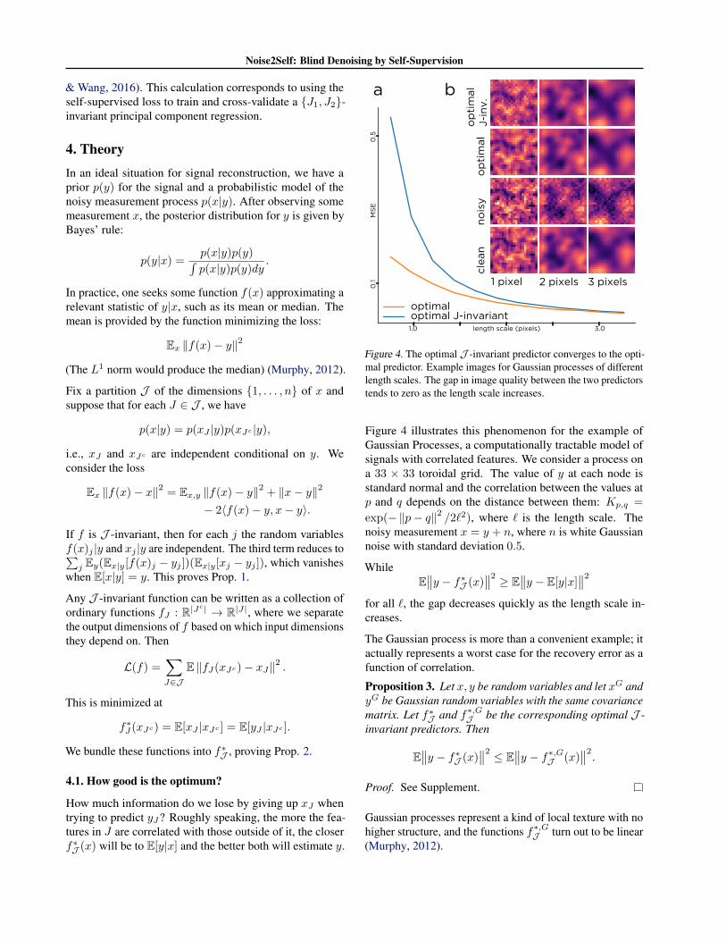
Figure 4. The optimal J -invariant predictor converges to the opti-mal predictor. Example images for Gaussian processes of differentlength scales. The gap in image quality between the two predictorstends to zero as the length scale increases.

Figure 4 illustrates this phenomenon for the example ofGaussian Processes, a computationally tractable model ofsignals with correlated features. We consider a process ona 33 × 33 toroidal grid. The value of y at each node isstandard normal and the correlation between the values atp and q depends on the distance between them: Kp,q =

exp(−‖p− q‖2 /2`2), where ` is the length scale. Thenoisy measurement x = y + n, where n is white Gaussiannoise with standard deviation 0.5.

WhileE∥∥y − f∗J (x)∥∥2 ≥ E

∥∥y − E[y|x]∥∥2

for all `, the gap decreases quickly as the length scale in-creases.

The Gaussian process is more than a convenient example; itactually represents a worst case for the recovery error as afunction of correlation.

Proposition 3. Let x, y be random variables and let xG andyG be Gaussian random variables with the same covariancematrix. Let f∗J and f∗,GJ be the corresponding optimal J -invariant predictors. Then

E∥∥y − f∗J (x)∥∥2 ≤ E

∥∥y − f∗,GJ (x)∥∥2.

Proof. See Supplement.

Gaussian processes represent a kind of local texture with nohigher structure, and the functions f∗,GJ turn out to be linear(Murphy, 2012).

Noise2Self: Blind Denoising by Self-Supervision

0.2 0.4 0.6 0.8 1.0 1.2 1.4

0.01

0.03

Noise standard deviationclean

MS

E

Gaussian ProcessAlphabet

noisy optimally denoised

GaussianProcessof same covariance

Alphabet

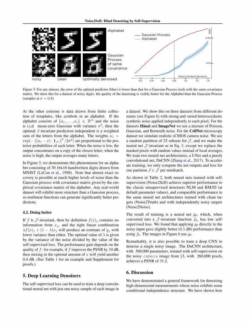
Figure 5. For any dataset, the error of the optimal predictor (blue) is lower than that for a Gaussian Process (red) with the same covariancematrix. We show this for a dataset of noisy digits: the quality of the denoising is visibly better for the Alphabet than the Gaussian Process(samples at σ = 0.8).

At the other extreme is data drawn from finite collec-tion of templates, like symbols in an alphabet. If thealphabet consists of {a1, . . . , ar} ∈ Rm and the noiseis i.i.d. mean-zero Gaussian with variance σ2, then theoptimal J-invariant prediction independent is a weightedsum of the letters from the alphabet. The weights wi =exp(−‖(ai − x) · 1Jc‖2 /2σ2) are proportional to the pos-terior probabilities of each letter. When the noise is low, theoutput concentrates on a copy of the closest letter; when thenoise is high, the output averages many letters.

In Figure 5, we demonstrate this phenomenon for an alpha-bet consisting of 30 16x16 handwritten digits drawn fromMNIST (LeCun et al., 1998). Note that almost exact re-covery is possible at much higher levels of noise than theGaussian process with covariance matrix given by the em-pirical covariance matrix of the alphabet. Any real-worlddataset will exhibit more structure than a Gaussian process,so nonlinear functions can generate significantly better pre-dictions.

4.2. Doing better

If f is J -invariant, then by definition f(x)j contains noinformation from xj , and the right linear combinationλf(x)j + (1 − λ)xj will produce an estimate of yj withlower variance than either. The optimal value of λ is givenby the variance of the noise divided by the value of theself-supervised loss. The performance gain depends on thequality of f : for example, if f improves the PSNR by 10 dB,then mixing in the optimal amount of x will yield another0.4 dB. (See Table 1 for an example and Supplement forproofs.)

5. Deep Learning DenoisersThe self-supervised loss can be used to train a deep convolu-tional neural net with just one noisy sample of each image in

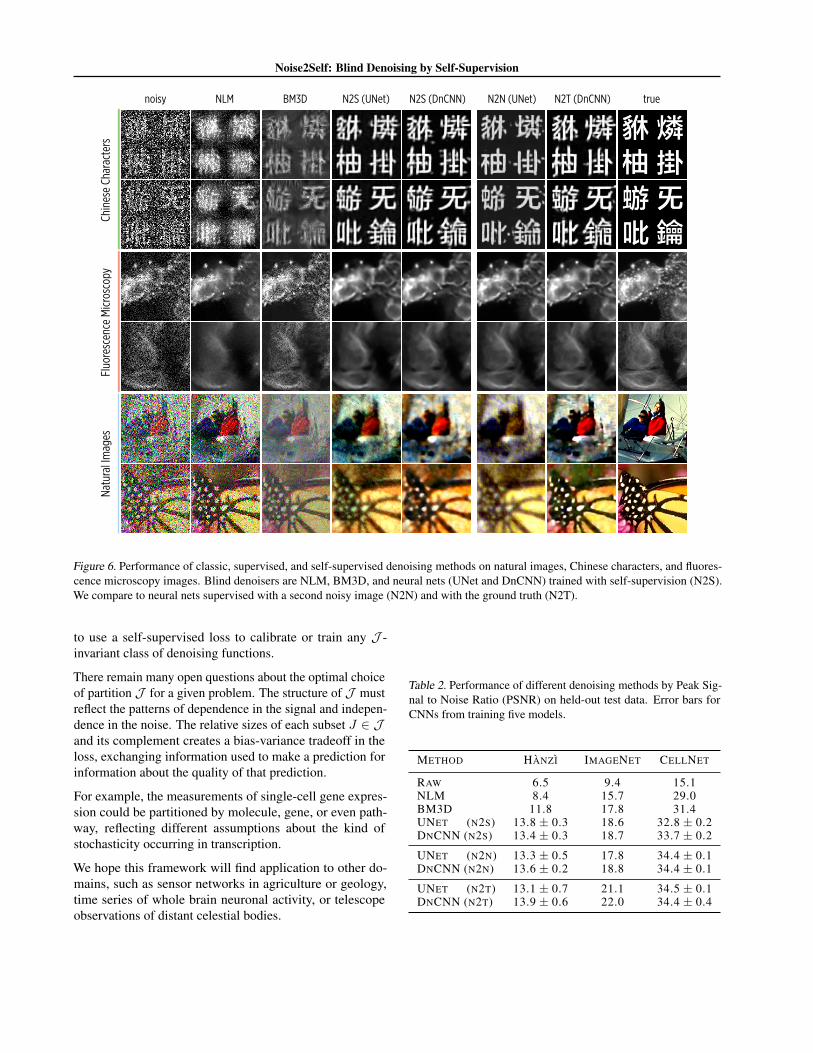
a dataset. We show this on three datasets from different do-mains (see Figure 6) with strong and varied heteroscedasticsynthetic noise applied independently to each pixel. For thedatasets Hanzı and ImageNet we use a mixture of Poisson,Gaussian, and Bernoulli noise. For the CellNet microscopydataset we simulate realistic sCMOS camera noise. We usea random partition of 25 subsets for J , and we make theneural net J -invariant as in Eq. 3, except we replace themasked pixels with random values instead of local averages.We train two neural net architectures, a UNet and a purelyconvolutional net, DnCNN (Zhang et al., 2017). To acceler-ate training, we only compute the net outputs and loss forone partition J ∈ J per minibatch.

As shown in Table 2, both neural nets trained with self-supervision (Noise2Self) achieve superior performance tothe classic unsupervised denoisers NLM and BM3D (atdefault parameter values), and comparable performance tothe same neural net architectures trained with clean tar-gets (Noise2Truth) and with independently noisy targets(Noise2Noise).

The result of training is a neural net gθ, which, whenconverted into a J -invariant function fθ, has low self-supervised loss. We found that applying gθ directly to thenoisy input gave slightly better (0.5 dB) performance thanusing fθ. The images in Figure 6 use gθ.

Remarkably, it is also possible to train a deep CNN todenoise a single noisy image. The DnCNN architecture,with 560,000 parameters, trained with self-supervision onthe noisy camera image from §3, with 260,000 pixels,achieves a PSNR of 31.2.

6. DiscussionWe have demonstrated a general framework for denoisinghigh-dimensional measurements whose noise exhibits someconditional independence structure. We have shown how

Noise2Self: Blind Denoising by Self-Supervision

truenoisy NLM BM3D N2T (DnCNN)N2S (DnCNN) N2N (UNet)Fl

uore

scen

ce M

icros

copy

Chin

ese

Char

acte

rsNa

tura

l Im

ages

N2S (UNet)

Figure 6. Performance of classic, supervised, and self-supervised denoising methods on natural images, Chinese characters, and fluores-cence microscopy images. Blind denoisers are NLM, BM3D, and neural nets (UNet and DnCNN) trained with self-supervision (N2S).We compare to neural nets supervised with a second noisy image (N2N) and with the ground truth (N2T).

to use a self-supervised loss to calibrate or train any J -invariant class of denoising functions.

There remain many open questions about the optimal choiceof partition J for a given problem. The structure of J mustreflect the patterns of dependence in the signal and indepen-dence in the noise. The relative sizes of each subset J ∈ Jand its complement creates a bias-variance tradeoff in theloss, exchanging information used to make a prediction forinformation about the quality of that prediction.

For example, the measurements of single-cell gene expres-sion could be partitioned by molecule, gene, or even path-way, reflecting different assumptions about the kind ofstochasticity occurring in transcription.

We hope this framework will find application to other do-mains, such as sensor networks in agriculture or geology,time series of whole brain neuronal activity, or telescopeobservations of distant celestial bodies.

Table 2. Performance of different denoising methods by Peak Sig-nal to Noise Ratio (PSNR) on held-out test data. Error bars forCNNs from training five models.

METHOD HANZI IMAGENET CELLNET

RAW 6.5 9.4 15.1NLM 8.4 15.7 29.0BM3D 11.8 17.8 31.4UNET (N2S) 13.8 ± 0.3 18.6 32.8 ± 0.2DNCNN (N2S) 13.4 ± 0.3 18.7 33.7 ± 0.2

UNET (N2N) 13.3 ± 0.5 17.8 34.4 ± 0.1DNCNN (N2N) 13.6 ± 0.2 18.8 34.4 ± 0.1

UNET (N2T) 13.1 ± 0.7 21.1 34.5 ± 0.1DNCNN (N2T) 13.9 ± 0.6 22.0 34.4 ± 0.4

Noise2Self: Blind Denoising by Self-Supervision

AcknowledgementsThank you to James Webber, Jeremy Freeman, DavidDynerman, Nicholas Sofroniew, Jaakko Lehtinen, JennyFolkesson, Anitha Krishnan, and Vedran Hadziosmanovicfor valuable conversations. Thank you to Jack Kamm fordiscussions on Gaussian Processes and shrinkage estima-tors. Thank you to Martin Weigert for his help runningBM3D. Thank you to the referees for suggesting valuableclarifications. Thank you to the Chan Zuckerberg Biohubfor financial support.

ReferencesBro, R., Kjeldahl, K., Smilde, A. K., and Kiers, H. A. L.

Cross-validation of component models: A critical look atcurrent methods. Analytical and Bioanalytical Chemistry,390(5):1241–1251, March 2008.

Buades, A., Coll, B., and Morel, J.-M. A non-local algo-rithm for image denoising. In 2005 IEEE Computer Soci-ety Conference on Computer Vision and Pattern Recogni-tion (CVPR’05), volume 2, pp. 60–65. IEEE, 2005a.

Buades, A., Coll, B., and Morel, J.-M. A review of im-age denoising algorithms, with a new one. MultiscaleModeling & Simulation, 4(2):490–530, 2005b.

Chang, S. G., Yu, B., and Vetterli, M. Adaptive waveletthresholding for image denoising and compression. IEEEtransactions on image processing, 9(9):1532–1546, 2000.

Dabov, K., Foi, A., Katkovnik, V., and Egiazarian, K. Imagedenoising by sparse 3-D transform-domain collaborativefiltering. IEEE Transactions on Image Processing, 16(8):2080–2095, August 2007.

Ehret, T., Davy, A., Facciolo, G., Morel, J.-M., and Arias, P.Model-blind video denoising via frame-to-frame training.arXiv:1811.12766 [cs], November 2018.

Elad, M. and Aharon, M. Image denoising via sparse andredundant representations over learned dictionaries. IEEETransactions on Image Processing, 15(12):3736–3745,December 2006.

Gallinari, P., Lecun, Y., Thiria, S., and Soulie, F. Memoiresassociatives distribuees: Une comparaison (Distributedassociative memories: A comparison). Proceedings ofCOGNITIVA 87, Paris, La Villette, May 1987, 1987.

Krull, A., Buchholz, T.-O., and Jug, F. Noise2Void- learning denoising from single noisy images.arXiv:1811.10980 [cs], November 2018.

Lebrun, M. An analysis and implementation of the BM3Dimage denoising method. Image Processing On Line, 2:175–213, August 2012.

LeCun, Y., Bottou, L., Bengio, Y., and Haffner, P. Gradient-based learning applied to document recognition. Proceed-ings of the IEEE, 86(11):2278–2324, 1998.

Lehtinen, J., Munkberg, J., Hasselgren, J., Laine, S., Karras,T., Aittala, M., and Aila, T. Noise2Noise: Learningimage restoration without clean data. In InternationalConference on Machine Learning, pp. 2971–2980, 2018.

Ljosa, V., Sokolnicki, K. L., and Carpenter, A. E. Annotatedhigh-throughput microscopy image sets for validation.Nature Methods, 9(7):637–637, July 2012.

Metzler, C. A., Mousavi, A., Heckel, R., and Baraniuk,R. G. Unsupervised learning with Stein’s unbiased riskestimator. arXiv:1805.10531 [cs, stat], May 2018.

Milo, R., Jorgensen, P., Moran, U., Weber, G., and Springer,M. BioNumbers – the database of key numbers in molecu-lar and cell biology. Nucleic Acids Research, 38(suppl 1):D750–D753, January 2010.

Murphy, K. P. Machine Learning: a Probabilistic Perspec-tive. Adaptive computation and machine learning series.MIT Press, Cambridge, MA, 2012. ISBN 978-0-262-01802-9.

Owen, A. B. and Perry, P. O. Bi-cross-validation of the SVDand the nonnegative matrix factorization. The Annals ofApplied Statistics, 3(2):564–594, June 2009.

Owen, A. B. and Wang, J. Bi-cross-validation for factoranalysis. Statistical Science, 31(1):119–139, 2016.

Papyan, V., Romano, Y., Sulam, J., and Elad, M. Con-volutional dictionary learning via local processing.arXiv:1705.03239 [cs], May 2017.

Paszke, A., Gross, S., Chintala, S., Chanan, G., Yang, E.,DeVito, Z., Lin, Z., Desmaison, A., Antiga, L., and Lerer,A. Automatic differentiation in PyTorch. In NIPS-W,2017.

Paul, F., Arkin, Y., Giladi, A., Jaitin, D., Kenigsberg, E.,Keren-Shaul, H., Winter, D., Lara-Astiaso, D., Gury, M.,Weiner, A., David, E., Cohen, N., Lauridsen, F., Haas, S.,Schlitzer, A., Mildner, A., Ginhoux, F., Jung, S., Trumpp,A., Porse, B., Tanay, A., and Amit, I. Transcriptionalheterogeneity and lineage commitment in myeloid pro-genitors. Cell, 163(7):1663–1677, December 2015.

Pennebaker, W. B. and Mitchell, J. L. JPEG still image datacompression standard. Van Nostrand Reinhold, NewYork, 1992. ISBN 978-0-442-01272-4.

Ronneberger, O., Fischer, P., and Brox, T. U-Net: Con-volutional networks for biomedical image segmentation.arXiv:1505.04597 [cs], May 2015.

Noise2Self: Blind Denoising by Self-Supervision

Tripathi, S., Lipton, Z. C., and Nguyen, T. Q. Correction byprojection: Denoising images with generative adversarialnetworks. arXiv:1803.04477 [cs], March 2018.

Ulyanov, D., Vedaldi, A., and Lempitsky, V. Deep imageprior. arXiv:1711.10925 [cs, stat], November 2017.

van der Walt, S., Schnberger, J. L., Nunez-Iglesias, J.,Boulogne, F., Warner, J. D., Yager, N., Gouillart, E.,Yu, T., and contributors, t. s.-i. scikit-image: image pro-cessing in Python. PeerJ, 2:e453, 2014.

van Dijk, D., Sharma, R., Nainys, J., Yim, K., Kathail, P.,Carr, A. J., Burdziak, C., Moon, K. R., Chaffer, C. L.,Pattabiraman, D., Bierie, B., Mazutis, L., Wolf, G., Krish-naswamy, S., and Peer, D. Recovering gene interactionsfrom single-cell data using data diffusion. Cell, 174(3):716–729.e27, July 2018.

Vincent, P., Larochelle, H., Lajoie, I., Bengio, Y., and Man-zagol, P.-A. Stacked denoising autoencoders: Learninguseful representations in a deep network with a local de-noising criterion. Journal of machine learning research,11(Dec):3371–3408, 2010.

Weigert, M., Schmidt, U., Boothe, T., Mller, A., Dibrov,A., Jain, A., Wilhelm, B., Schmidt, D., Broaddus, C.,Culley, S., Rocha-Martins, M., Segovia-Miranda, F., Nor-den, C., Henriques, R., Zerial, M., Solimena, M., Rink,J., Tomancak, P., Royer, L., Jug, F., and Myers, E. W.Content-Aware image restoration: Pushing the limits offluorescence microscopy. July 2018.

Zhang, K., Zuo, W., Chen, Y., Meng, D., and Zhang, L.Beyond a Gaussian denoiser: Residual learning of deepCNN for image denoising. IEEE Transactions on ImageProcessing, 26(7):3142–3155, July 2017.

Zhussip, M., Soltanayev, S., and Chun, S. Y. Trainingdeep learning based image denoisers from undersampledmeasurements without ground truth and without imageprior. arXiv:1806.00961 [cs], June 2018.