Nonconvex Rigid Bodies with Stacking

Eran Guendelman∗

Stanford UniversityRobert Bridson∗

Stanford UniversityRonald Fedkiw†

Stanford University

Abstract

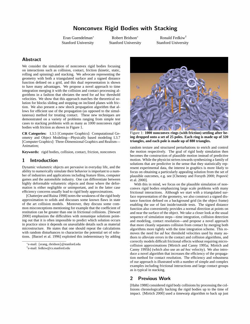
We consider the simulation of nonconvex rigid bodies focusingon interactions such as collision, contact, friction (kinetic, static,rolling and spinning) and stacking. We advocate representing thegeometry with both a triangulated surface and a signed distancefunction defined on a grid, and this dual representation is shownto have many advantages. We propose a novel approach to timeintegration merging it with the collision and contact processing al-gorithms in a fashion that obviates the need forad hoc thresholdvelocities. We show that this approach matches the theoretical so-lution for blocks sliding and stopping on inclined planes with fric-tion. We also present a new shock propagation algorithm that al-lows for efficient use of the propagation (as opposed to the simul-taneous) method for treating contact. These new techniques aredemonstrated on a variety of problems ranging from simple testcases to stacking problems with as many as 1000 nonconvex rigidbodies with friction as shown in Figure 1.

CR Categories: I.3.5 [Computer Graphics]: Computational Ge-ometry and Object Modeling—Physically based modeling I.3.7[Computer Graphics]: Three-Dimensional Graphics and Realism—Animation;

Keywords: rigid bodies, collision, contact, friction, nonconvex

1 Introduction

Dynamic volumetric objects are pervasive in everyday life, and theability to numerically simulate their behavior is important to a num-ber of industries and applications including feature films, computergames and the automobile industry. One can differentiate betweenhighly deformable volumetric objects and those where the defor-mation is either negligible or unimportant, and in the latter caseefficiency concerns usually lead to rigid body approximations.

[Chatterjee and Ruina 1998] notes the weakness of the rigid bodyapproximation to solids and discusses some known flaws in stateof the art collision models. Moreover, they discuss some com-mon misconceptions mentioning for example that the coefficient ofrestitution can be greater than one in frictional collisions. [Stewart2000] emphasizes the difficulties with nonunique solutions point-ing out that it is often impossible to predict which solution occursin practice since it depends on unavailable details such as materialmicrostructure. He states that one should repeat the calculationswith random disturbances to characterize the potential set of solu-tions. [Barzel et al. 1996] exploited this indeterminacy by adding

∗e-mail:{erang, rbridson}@stanford.edu†e-mail: fedkiw@cs.stanford.edu

Figure 1:1000 nonconvex rings (with friction) settling after be-ing dropped onto a set of 25 poles. Each ring is made up of 320triangles, and each pole is made up of 880 triangles.

random texture and structured perturbations to enrich and controlthe motion respectively. The goal of rigid body simulation thenbecomes the construction of plausible motion instead of predictivemotion. While the physicist strives towards synthesizing a family ofsolutions that are predictive in the sense that they statistically rep-resent experimental data, the interest in graphics is more likely tofocus on obtaining a particularly appealing solution from the set ofplausible outcomes, e.g. see [Chenney and Forsyth 2000; Popovicet al. 2000].

With this in mind, we focus on the plausible simulation of non-convex rigid bodies emphasizing large scale problems with manyfrictional interactions. Although we start with a triangulated sur-face representation of the geometry, we also construct a signed dis-tance function defined on a background grid (in the object frame)enabling the use of fast inside/outside tests. The signed distancefunction also conveniently provides a normal direction at points onand near the surface of the object. We take a closer look at the usualsequence of simulation steps—time integration, collision detectionand modeling, contact resolution—and propose a novel approachthat more cleanly separates collision from contact by merging bothalgorithms more tightly with the time integration scheme. This re-moves the need forad hoc threshold velocities used by many au-thors to alleviate errors in the contact and collision algorithms, andcorrectly models difficult frictional effects without requiring micro-collision approximations [Mirtich and Canny 1995a; Mirtich andCanny 1995b] (which also use anad hoc velocity). We also intro-duce a novel algorithm that increases the efficiency of the propaga-tion method for contact resolution. The efficiency and robustnessof our approach is illustrated with a number of simple and complexexamples including frictional interactions and large contact groupsas is typical in stacking.

2 Previous Work

[Hahn 1988] considered rigid body collisions by processing the col-lisions chronologically backing the rigid bodies up to the time ofimpact. [Mirtich 2000] used a timewarp algorithm to back up just

the objects that are involved in collisions while still evolving non-colliding objects forward in time. This method works well exceptwhen there are a large number of bodies in contact groups, whichis the case we are concerned with in this paper. [Hahn 1988] pro-cessed collisions with static friction if the result was in the frictioncone, and otherwise used kinetic friction. If the approach veloc-ity was smaller than a threshold, the objects were assumed to be incontact and the same equations were applied approximating con-tinuous contact with a series of “instantaneous contacts”. [Mooreand Wilhelms 1988] instead proposed the use of repulsion forcesfor contact only using the exact impulse-based treatment for highvelocity collisions.

[Baraff 1989] proposed a method for analytically calculatingnon-colliding contact forces between polygonal objects obtainingan NP-hard quadratic programming problem which was solved us-ing a heuristic approach. He also points out that these ideas couldbe useful in collision propagation problems such as one billiard ballhitting a number of others (that are lined up) or objects falling in astack. [Baraff 1990] extended these concepts to curved surfaces.[Baraff 1991] advocated finding either a valid set of contact forcesor a valid set of contact impulses stressing that the usual preferenceof the latter only when the former does not exist may be misplaced.For more details, see [Baraff 1993]. [Baraff 1994] proposed a sim-pler, faster and more robust algorithm for solving these types ofproblems without the use of numerical optimization software.

[Bhatt and Koechling 1995] discussed the nonlinear differen-tial equations that need to be numerically integrated to analyzethe behavior of three-dimensional frictional rigid body impact andpointed out that the problem becomes ill-conditioned at the stickingpoint. Then they use analysis to enumerate all the possible post-sticking scenarios and discuss the factors that determine a specificresult. [Mirtich and Canny 1995b] integrated these same nonlineardifferential equations to model both contact and collision propos-ing a unified model (as did [Hahn 1988]). They use the velocityan object at rest will obtain by falling through the collision enve-lope (or some threshold in [Mirtich and Canny 1995a]) to identifythe contact case and apply a microcollision model that reverses therelative velocity as long as the required impulse lies in the frictioncone. This solves the problem of blocks erroneously sliding downinclined planes due to impulse trains that cause them to spend timein a ballistic phase.

Implicitly defined surfaces were used for collision modeling by[Terzopoulos et al. 1987] to create repulsive force fields around ob-jects and [Pentland and Williams 1989; Sclaroff and Pentland 1991]who exploited fast inside/outside tests. We use a particular implicitsurface approach defining a signed distance function on an under-lying grid. Grid-based distance functions have been gaining popu-larity, see e.g. [Fisher and Lin 2001; Hirota et al. 2001] who usedthem to treat collision between deformable bodies, and [Kim andNeumann 2002] who used them to keep hair from interpenetratingthe head. Although [Gibson 1998] pointed out potential difficultieswith spurious minima in concave regions, we have not noticed anyadverse effects, most likely because we do not use repulsion forces.

[Milenkovic 1996] used position based physics to simulate thestacking of convex objects and discussed ways of making the simu-lations appear more physically realistic. [Milenkovic and Schmidl2001] considered stacking with standard Newtonian physics usingan optimization based method to adjust the predicted positions ofthe bodies to avoid overlap. One drawback is that the proceduretends to align bodies nonphysically. Quadratic programming isused for contact, collision and the position updates. They considerup to 1000 frictionless spheres, but nonconvex objects can only beconsidered as unions of convex objects and they indicate that thecomputational cost scales with the number of convex pieces. Theironly nonconvex example considered 50 jacks that were each theunion of 3 boxes. More recently, [Schmidl 2002] described a freez-

ing technique that identifies when objects can be removed from thesimulation, as well as identifying when to add them back. This al-lows the stacking of 1000 cubes with friction in 1.5 days as opposedto an estimated 45 days for simulating all the cubes.

3 Geometric Representation

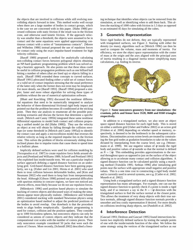
Since rigid bodies do not deform, they are typically representedwith triangulated surfaces, see Figure 2. Starting with either thedensity (or mass), algorithms such as [Mirtich 1996] can then beused to compute the volume, mass and moments of inertia. Forefficiency, we store the object space representation with the centerof mass at the origin and the axes aligned with the principal axesof inertia resulting in a diagonal inertia tensor simplifying manycalculations, e.g. finding its inverse.

Figure 2:Some nonconvex geometry from our simulations: thecranium, pelvis and femur have 3520, 8680 and 8160 trianglesrespectively.

In addition to a triangulated surface, we also store an objectspace signed distance function for each rigid body. This is storedon either a uniform grid [Osher and Fedkiw 2002] or an octree grid[Frisken et al. 2000] depending on whether speed or memory, re-spectively, is deemed to be the bottleneck in the subsequent calcu-lations. Discontinuities across octree levels are treated by constrain-ing the fine grid nodes at gradation boundaries to take on the valuesdictated by interpolating from the coarse level, see e.g. [Wester-mann et al. 1999]. We use negative values ofφ inside the rigidbody and positive values ofφ outside so that the normal is definedasN = ∇φ . This embedding provides approximations to the nor-mal throughout space as opposed to just on the surface of the objectallowing us to accelerate many contact and collision algorithms. Asigned distance function can be calculated quickly using a march-ing method [Tsitsiklis 1995; Sethian 1996] after initializing gridpoints near the surface with appropriate small negative and positivevalues. This is a one time cost in constructing a rigid body modeland is currently used in several systems, see e.g. [Cutler et al. 2002;Museth et al. 2002].

Using both a triangulated surface and a signed distance functionrepresentation has many advantages. For example, one can use thesigned distance function to quickly check if a point is inside a rigidbody, and if so intersect a ray in theN = ∇φ direction with thetriangulated surface to find the surface normal at the closest point.This allows the treatment of very sharp objects with their true sur-face normals, although signed distance function normals provide asmoother and less costly representation if desired. For more detailson collisions involving sharp objects, see [Pandolfi et al. 2002].

4 Interference Detection

[Gascuel 1993; Desbrun and Gascuel 1995] found intersections be-tween two implicitly defined surfaces by testing the sample pointsof one with the inside/outside function of the other. We follow thesame strategy using the vertices of the triangulated surface as our

sample points. This test is not sufficient to detect all collisions, asedge-face collisions are missed when both edge vertices are out-side the implicit surface. Since the errors are proportional to theedge length, they can be ignored in a well resolved mesh with smalltriangles. However, when substantial, e.g. when simulating cubeswith only 12 triangles, we intersect the triangle edges with the zeroisocontour and flag the deepest point on the edge as an interpen-etrating sample point. Since we do not consider time dependentcollisions, fast moving objects might pass through each other. Wealleviate this problem by limiting the size of a time step based onthe translational and rotational velocities of the objects and the sizeof their bounding boxes, although methods exist for treating the en-tire time swept path as a single implicit surface [Schroeder et al.1994].

A number of accelerations can be used in the interference de-tection process. For example, the inside/outside tests can be accel-erated by labeling the voxels that are completely inside and com-pletely outside (this is done for voxels at each level in the octreerepresentation as well) so that interpolation can be avoided exceptin cells which contain part of the interface. Labeling the mini-mum and maximum values ofφ in each voxel can also be useful.Bounding boxes and spheres are used around each object in order toprune points before doing a full inside/outside test. Moreover, if thebounding volumes are disjoint, no inside/outside tests are needed.For rigid bodies with a large number of triangles, we found an in-ternal box hierarchy with triangles in leaf boxes to be useful espe-cially when doing edge intersection tests. Also, we use a uniformspatial partitioning data structure with local memory storage imple-mented using a hash table in order to quickly narrow down whichrigid bodies might be intersecting. Similar spatial partitioning wasused in, for example, [Mirtich and Canny 1995b]. Again, we stressour interest in nonconvex objects and refer the reader to [Ponamgiet al. 1995; Kim et al. 2002] for other algorithms that treat arbitrarynonconvex polyhedral models. For more details on collision detec-tion methods, see e.g. [Webb and Gigante 1992; Lin and Gottschalk1998; Redon et al. 2002].

5 Time Integration

The equations for rigid body evolution are

xt = v, qt = 12ωq (1)

vt = F/m, Lt = τ (2)

wherex andq are the position and orientation (a unit quaternion),v andω are the velocity and angular velocity,F is the net force,mis the mass,L = Iω is the angular momentum with inertia tensorI = RDRT (R is the orientation matrix andD is the diagonal inertiatensor in object space), andτ is the net torque. For simplicity wewill considerF = mg and thusvt = g throughout the text, but ouralgorithm is not restricted to this case. While there are a number ofhighly accurate time integration methods for noninteracting rigidbodies in free flight, see e.g. [Buss 2000], these algorithms do notretain this accuracy in the presence of contact and collision. Thus,we take a different approach to time integration instead optimizingthe treatment of contact and collision. Moreover, we use a simpleforward Euler time integration for equations 1 and 2.

The standard approach is to integrate equations 1 and 2 forwardin time, and subsequently treat collision and then contact. Generallyspeaking, collisions require impulses that discontinuously modifythe velocity, and contacts are associated with forces and accelera-tions. However, friction can require the use of impulsive forces inthe contact treatment, although theprinciple of constraints requiresthat the use of impulsive forces be kept to a minimum. [Baraff1991] suggested that this avoidance of impulsive behavior is nei-ther necessary nor justified and stressed that there are algorithmicadvantages to using impulses exclusively. This naturally leads tosome blurring between collision and contact handling, and provides

a sense of justification to the work of [Hahn 1988] where the samealgebraic equations were used for both and the work of [Mirtichand Canny 1995b] who integrated the same nonlinear differentialequations for both. However, other authors such as [Moore andWilhelms 1988; Sims 1994; Kokkevis et al. 1996] have noted dif-ficulties associated with this blurring and proposed that an impulsebased treatment of collisions be separated from a penalty springsapproach to contact. They used the magnitude of the relative ve-locity to differentiate between contact and collision. [Mirtich andCanny 1995b] used the velocity an object at rest will obtain byfalling through the collision envelope (or some threshold in [Mir-tich and Canny 1995a]) to identify the contact case and applied amicrocollision model where the impulse needed to reverse the rel-ative velocity is applied as long as it lies in the friction cone. Theyshowed that this solves the problem of blocks erroneously slidingdown inclined planes due to impulse trains that cause them to spendtime in a ballistic phase.

A novel aspect of our approach is the clean separation of col-lision from contact without the need for threshold velocities. Wepropose the following time sequencing:

• Collision detection and modeling.• Advance the velocities using equation 2.• Contact resolution.• Advance the positions using equation 1.

The advantages of this time stepping scheme are best realizedthrough an example. Consider a block sitting still on an inclinedplane with a large coefficient of restitution, sayε = 1, and supposethat friction is large enough that the block should sit still. In a stan-dard time stepping scheme, both position and velocity are updatedfirst, followed by collision and contact resolution. During the po-sition and velocity update, the block starts to fall under the effectsof gravity. Then in the collision processing stage we detect a lowvelocity collision between the block and the plane, and sinceε = 1the block will change direction and bounce upwards at an angledown the incline. Then in the contact resolution stage, the blockand the plane are separating so nothing happens. The block willeventually fall back to the inclined plane, and continue bouncingup and down incorrectly sliding down the inclined plane becauseof the time it spends in the ballistic phase. This is the same phe-nomenon that causes objects sitting on the ground to vibrate as theyare incorrectly subjected to a number of elastic collisions. Thus,many authors usead hoc threshold velocities in an attempt to prunethese cases out of the collision modeling algorithm and instead treatthem with a contact model.

Our new time stepping algorithm automatically treats thesecases. All objects at rest have zero velocities (up to round-off error),so in the collision processing stage we do not get an elastic bounce(up to round-off error). Next, gravity is integrated into the velocity,and then the contact resolution algorithm correctly stops the objectsso that they remain still. Thus, nothing happens in the last (positionupdate) step, and we repeat the process. The key to the algorithm isthat contact modeling occurs directly after the velocity is updatedwith gravity. If instead either the collision step or a position updatewere to follow the velocity update, objects at rest will either incor-rectly elastically bounce or move through the floor, respectively. Onthe other hand, contact processing is the correct algorithm to applyafter the velocity update since it resolves forces, and the velocityupdate is where the forces are included in the dynamics.

One must use care when updating the velocity in between thecollision and contact algorithms to ensure that the same exact tech-nique is used to detect contact as was used to detect collision. Oth-erwise, an object in free flight might not register a collision, haveits velocity updated, and then register a contact causing it to incor-rectly receive an inelastic (instead of elastic) bounce. We avoid thissituation by guaranteeing that the contact detection step registers anegative result whenever the collision detection step does. This is

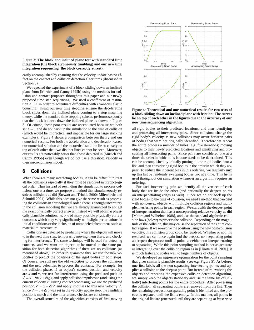
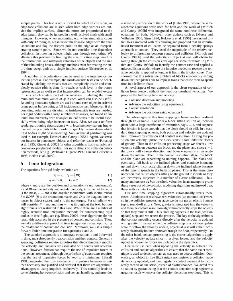
Figure 3:The block and inclined plane test with standard timeintegration (the block erroneously tumbling) and our new timeintegration sequencing (the block correctly at rest).

easily accomplished by ensuring that the velocity update has no ef-fect on the contact and collision detection algorithms (discussed inSection 6).

We repeated the experiment of a block sliding down an inclinedplane from [Mirtich and Canny 1995b] using the methods for col-lision and contact proposed throughout this paper and our newlyproposed time step sequencing. We used a coefficient of restitu-tion ε = 1 in order to accentuate difficulties with erroneous elasticbouncing. Using our new time stepping scheme the deceleratingblock slides down the inclined plane coming to a stop matchingtheory, while the standard time stepping scheme performs so poorlythat the block bounces down the inclined plane as shown in Figure3. Of course, these poor results are accentuated because we bothsetε = 1 and do not back up the simulation to the time of collision(which would be impractical and impossible for our large stackingexamples). Figure 4 shows a comparison between theory and ournumerical results. For both the acceleration and deceleration cases,our numerical solution and the theoretical solution lie so closely ontop of each other that two distinct lines cannot be seen. Moreover,our results are noticeably better than those depicted in [Mirtich andCanny 1995b] even though we do not use a threshold velocity ortheir microcollision model.

6 Collisions

When there are many interacting bodies, it can be difficult to treatall the collisions especially if they must be resolved in chronologi-cal order. Thus instead of rewinding the simulation to process col-lisions one at a time, we propose a method that simultaneously re-solves collisions as did [Stewart and Trinkle 2000; Milenkovic andSchmidl 2001]. While this does not give the same result as process-ing the collisions in chronological order, there is enough uncertaintyin the collision modeling that we are already guaranteed to not getthe exact physically correct answer. Instead we will obtaina physi-cally plausible solution, i.e. one of many possible physically correctoutcomes which may vary significantly with slight perturbations ininitial conditions or the inclusion of unmodeled phenomena such asmaterial microstructure.

Collisions are detected by predicting where the objects will moveto in the next time step, temporarily moving them there, and check-ing for interference. The same technique will be used for detectingcontacts, and we want the objects to be moved to the same po-sition for both detection algorithms if there are no collisions (asmentioned above). In order to guarantee this, we use the new ve-locities to predict the positions of the rigid bodies in both steps.Of course, we still use the old velocities to process the collisionsand the new velocities to process the contacts. For example, forthe collision phase, if an object’s current position and velocityare x and v, we test for interference using the predicted positionx′ = x+∆t(v+∆tg), and apply collision impulses to (and using) thecurrent velocityv. During contact processing, we use the predictedpositionx′ = x + ∆tv′ and apply impulses to this new velocityv′.Sincev′ = v+∆tg was set in the velocity update step, the candidatepositions match and the interference checks are consistent.

The overall structure of the algorithm consists of first moving

Decelerating Down Ramp

0.0 0.5 1.0 1.5 2.00.0

0.1

0.2

0.3

0.4

0.5

0.6

0.7

time(s)

pos

(m)

Decelerating Down Ramp

0.0 0.5 1.0 1.5 2.00.0

0.2

0.4

0.6

0.8

1.0

1.2

1.4

time(s)

vel (

m/s

)

Accelerating Down Ramp

0.0 0.5 1.0 1.5 2.00.0

0.5

1.0

1.5

2.0

2.5

time(s)

pos

(m)

Accelerating Down Ramp

0.0 0.5 1.0 1.5 2.00.0

0.5

1.0

1.5

2.0

2.5

time(s)

vel (

m/s

)

Figure 4:Theoretical and our numerical results for two tests ofa block sliding down an inclined plane with friction. The curveslie on top of each other in the figures due to the accuracy of ournew time sequencing algorithm.

all rigid bodies to their predicted locations, and then identifyingand processing all intersecting pairs. Since collisions change therigid body’s velocity,v, new collisions may occur between pairsof bodies that were not originally identified. Therefore we repeatthe entire process a number of times (e.g. five iterations) movingobjects to their newly predicted locations and identifying and pro-cessing all intersecting pairs. Since pairs are considered one at atime, the order in which this is done needs to be determined. Thiscan be accomplished by initially putting all the rigid bodies into alist, and then considering rigid bodies in the order in which they ap-pear. To reduce the inherent bias in this ordering, we regularly mixup this list by randomly swapping bodies two at a time. This list isused throughout our simulation whenever an algorithm requires anordering.

For each intersecting pair, we identify all the vertices of eachbody that are inside the other (and optionally the deepest pointson interpenetrating edges as well). Since we do not back up therigid bodies to the time of collision, we need a method that can dealwith nonconvex objects with multiple collision regions and multi-ple interfering points in each region. We start with the deepest pointof interpenetration that has a nonseparating relative velocity as did[Moore and Wilhelms 1988], and use the standard algebraic colli-sion laws (below) to process the collision. Depending on the magni-tude of the collision, this may cause the separation of the entire con-tact region. If we re-evolve the position using the new post-collisionvelocity, this collision group could be resolved. Whether or not it isresolved, we can once again find the deepest non-separating pointand repeat the process until all points are either non-interpenetratingor separating. While this point sampling method is not as accurateas integrating over the collision region as in [Hirota et al. 2001], itis much faster and scales well to large numbers of objects.

We developed an aggressive optimization for the point samplingthat gives similarly plausible results, (see e.g. Figure 5). As before,one first labels all the non-separating intersecting points and ap-plies a collision to the deepest point. But instead of re-evolving theobjects and repeating the expensive collision detection algorithm,we simply keep the objects stationary and use the same list of (ini-tially) interfering points for the entire procedure. After processingthe collision, all separating points are removed from the list. Thenthe remaining deepest nonseparating point is identified and the pro-cess is repeated until the list is empty. In this manner, all points inthe original list are processed until they are separatingat least once

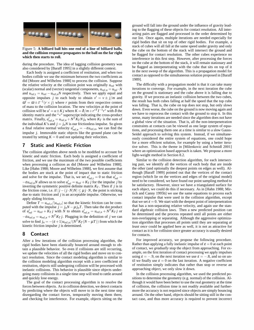
Figure 5: A billiard ball hits one end of a line of billiard balls,and the collision response propagates to the ball on the far rightwhich then starts to roll.

during the procedure. The idea of lagging collision geometry wasalso considered by [Baraff 1995] in a slightly different context.

Each body is assigned a coefficient of restitution, and when twobodies collide we use the minimum between the two coefficients asdid [Moore and Wilhelms 1988] to process the collision. Supposethe relative velocity at the collision point was originallyurel with(scalar) normal and (vector) tangential components,urel,n = urel ·Nandurel,t = urel − urel,nN respectively. Then we apply equal andopposite impulsesj to each body to obtainv′ = v ± j/m andω ′ = ω ± I−1(r × j) wherer points from their respective centersof mass to the collision location. The new velocities at the point ofcollision will beu′ = u±K j whereK = δ/m+r∗T I−1r∗ with δ theidentity matrix and the “∗” superscript indicating the cross-productmatrix. Finally,u′rel,n = urel,n + NT KT N jn whereKT is the sum ofthe individualK’s and j = jnN is our frictionless impulse. So givena final relative normal velocityu′rel,n = −εurel,n, we can find theimpulse j. Immovable static objects like the ground plane can betreated by settingK = 0 and not updating their velocities.

7 Static and Kinetic Friction

The collision algorithm above needs to be modified to account forkinetic and static friction. Each body is assigned a coefficient offriction, and we use the maximum of the two possible coefficientswhen processing a collision as did [Moore and Wilhelms 1988].Like [Hahn 1988; Moore and Wilhelms 1988], we first assume thatthe bodies are stuck at the point of impact due to static frictionand solve for the impulse. That is, we setu′rel,t = 0 so thatu′rel =

−εurel,nN allows us to solveu′rel = urel +KT j for the impulsej byinverting the symmetric positive definite matrixKT . Then if j is inthe friction cone, i.e. if| j− ( j ·N)N| ≤ µ j ·N, the point is stickingdue to static friction andj is an acceptable impulse. Otherwise, weapply sliding friction.

DefineT = urel,t/|urel,t | so that the kinetic friction can be com-puted with the impulsej = jnN −µ jnT . Then take the dot productof u′rel = urel + KT j with N to obtainu′rel,n = urel,n + NT KT j or

−εurel,n = urel,n + NT KT j. Plugging in the definition ofj we cansolve to findjn =−(ε +1)urel,n/(NT KT (N−µT )) from which thekinetic friction impulsej is determined.

8 Contact

After a few iterations of the collision processing algorithm, therigid bodies have been elastically bounced around enough to ob-tain a plausible behavior. So even if collisions are still occurring,we update the velocities of all the rigid bodies and move on to con-tact resolution. Since the contact modeling algorithm is similar tothe collision modeling algorithm except with a zero coefficient ofrestitution, objects still undergoing collision will be processed withinelastic collisions. This behavior is plausible since objects under-going many collisions in a single time step will tend to rattle aroundand quickly lose energy.

The goal of the contact processing algorithm is to resolve theforces between objects. As in collision detection, we detect contactsby predicting where the objects will move to in the next time stepdisregarding the contact forces, temporarily moving them there,and checking for interference. For example, objects sitting on the

ground will fall into the ground under the influence of gravity lead-ing to the flagging of these objects for contact resolution. All inter-acting pairs are flagged and processed in the order determined byour list. Once again, multiple iterations are needed especially forrigid bodies that sit on top of other rigid bodies. For example, astack of cubes will all fall at the same speed under gravity and onlythe cube on the bottom of the stack will intersect the ground andbe flagged for contact resolution. The other cubes experience nointerference in this first step. However, after processing the forceson the cube at the bottom of the stack, it will remain stationary andbe flagged as interpenetrating with the cube that sits on top of itin the next sweep of the algorithm. This is a propagation model forcontact as opposed to the simultaneous solution proposed in [Baraff1989].

The difficulty with a propagation model is that it can take manyiterations to converge. For example, in the next iteration the cubeon the ground is stationary and the cube above it is falling due togravity. If we process an inelastic collision between the two cubes,the result has both cubes falling at half the speed that the top cubewas falling. That is, the cube on top does not stop, but only slowsdown. Even worse, the cube on the ground is now moving again andwe have to reprocess the contact with the ground to stop it. In thissense, many iterations are needed since the algorithm does not havea global view of the situation. That is, all the non-interpenetrationconstraints at contacts can be viewed as one large system of equa-tions, and processing them one at a time is similar to a slow Gauss-Seidel approach to solving this system. Instead, if we simultane-ously considered the entire system of equations, one could hopefor a more efficient solution, for example by using a better itera-tive solver. This is the theme in [Milenkovic and Schmidl 2001]where an optimization based approach is taken. We propose a morelight-weight method in Section 8.2.

Similar to the collision detection algorithm, for each intersect-ing pair, we identify all the vertices of each body that are insidethe other (and optionally the deepest points on edges as well). Al-though [Baraff 1989] pointed out that the vertices of the contactregion (which lie on the vertices and edges of the original model)need to be considered, we have found our point sampling method tobe satisfactory. However, since we have a triangulated surface foreach object, we could do this if necessary. As in [Hahn 1988; Mir-tich and Canny 1995b] we use the same equations to process eachcontact impulse that were used in the collision algorithm, exceptthat we setε = 0. We start with the deepest point of interpenetrationthat has a non-separating relative velocity, and again use the stan-dard algebraic collision laws. Then a new predicted position canbe determined and the process repeated until all points are eithernon-overlapping or separating. Although the aggressive optimiza-tion algorithm that processes all points until they are separatingatleast once could be applied here as well, it is not as attractive forcontact as it is for collision since greater accuracy is usually desiredfor contacts.

For improved accuracy, we propose the following procedure.Rather than applying a fully inelastic impulse ofε = 0 at each pointof contact, wegradually stop the object from approaching. For ex-ample, on the first iteration of contact processing we apply impulsesusingε = −.9, on the next iteration we useε = −.8, and so on un-til we finally useε = 0 on the last iteration. A negative coefficientof restitution simply indicates that rather than stop or reverse anapproaching object, we only slow it down.

In the collision processing algorithm, we used the predicted po-sitions to determine the geometry (e.g. normal) of the collision. Al-though it would have been better to use the real geometry at the timeof collision, the collision time is not readily available and further-more the accuracy is not required since objects are simply bouncingaround. On the other hand, objects should be sitting still in the con-tact case, and thus more accuracy is required to prevent incorrect

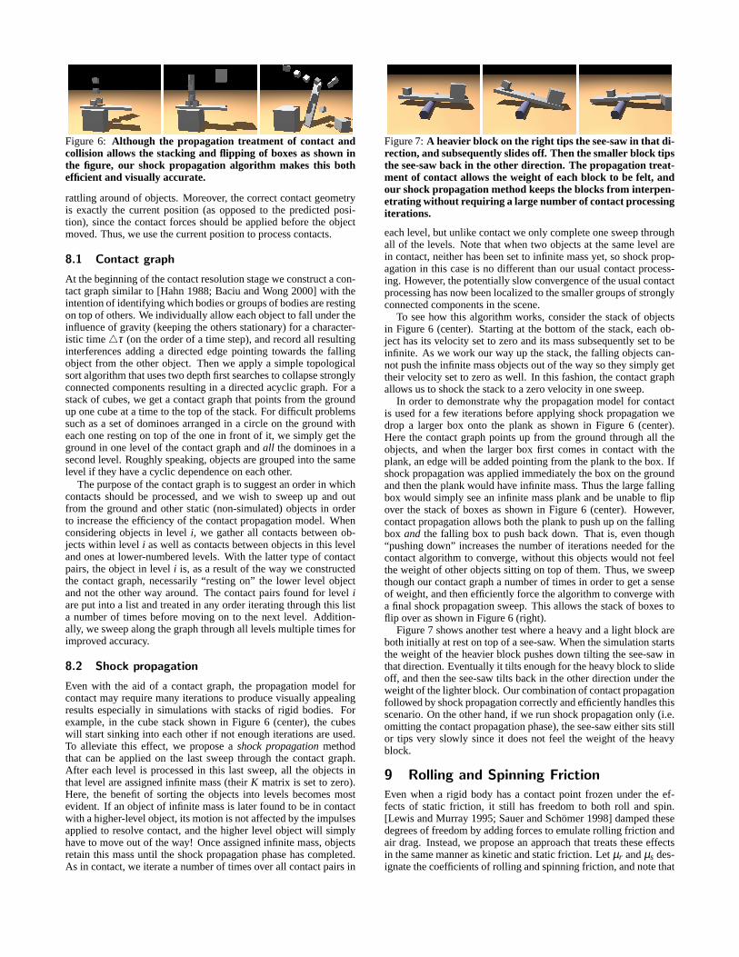
Figure 6: Although the propagation treatment of contact andcollision allows the stacking and flipping of boxes as shown inthe figure, our shock propagation algorithm makes this bothefficient and visually accurate.

rattling around of objects. Moreover, the correct contact geometryis exactly the current position (as opposed to the predicted posi-tion), since the contact forces should be applied before the objectmoved. Thus, we use the current position to process contacts.

8.1 Contact graph

At the beginning of the contact resolution stage we construct a con-tact graph similar to [Hahn 1988; Baciu and Wong 2000] with theintention of identifying which bodies or groups of bodies are restingon top of others. We individually allow each object to fall under theinfluence of gravity (keeping the others stationary) for a character-istic time4τ (on the order of a time step), and record all resultinginterferences adding a directed edge pointing towards the fallingobject from the other object. Then we apply a simple topologicalsort algorithm that uses two depth first searches to collapse stronglyconnected components resulting in a directed acyclic graph. For astack of cubes, we get a contact graph that points from the groundup one cube at a time to the top of the stack. For difficult problemssuch as a set of dominoes arranged in a circle on the ground witheach one resting on top of the one in front of it, we simply get theground in one level of the contact graph andall the dominoes in asecond level. Roughly speaking, objects are grouped into the samelevel if they have a cyclic dependence on each other.

The purpose of the contact graph is to suggest an order in whichcontacts should be processed, and we wish to sweep up and outfrom the ground and other static (non-simulated) objects in orderto increase the efficiency of the contact propagation model. Whenconsidering objects in leveli, we gather all contacts between ob-jects within leveli as well as contacts between objects in this leveland ones at lower-numbered levels. With the latter type of contactpairs, the object in leveli is, as a result of the way we constructedthe contact graph, necessarily “resting on” the lower level objectand not the other way around. The contact pairs found for leveliare put into a list and treated in any order iterating through this lista number of times before moving on to the next level. Addition-ally, we sweep along the graph through all levels multiple times forimproved accuracy.

8.2 Shock propagation

Even with the aid of a contact graph, the propagation model forcontact may require many iterations to produce visually appealingresults especially in simulations with stacks of rigid bodies. Forexample, in the cube stack shown in Figure 6 (center), the cubeswill start sinking into each other if not enough iterations are used.To alleviate this effect, we propose ashock propagation methodthat can be applied on the last sweep through the contact graph.After each level is processed in this last sweep, all the objects inthat level are assigned infinite mass (theirK matrix is set to zero).Here, the benefit of sorting the objects into levels becomes mostevident. If an object of infinite mass is later found to be in contactwith a higher-level object, its motion is not affected by the impulsesapplied to resolve contact, and the higher level object will simplyhave to move out of the way! Once assigned infinite mass, objectsretain this mass until the shock propagation phase has completed.As in contact, we iterate a number of times over all contact pairs in

Figure 7:A heavier block on the right tips the see-saw in that di-rection, and subsequently slides off. Then the smaller block tipsthe see-saw back in the other direction. The propagation treat-ment of contact allows the weight of each block to be felt, andour shock propagation method keeps the blocks from interpen-etrating without requiring a large number of contact processingiterations.

each level, but unlike contact we only complete one sweep throughall of the levels. Note that when two objects at the same level arein contact, neither has been set to infinite mass yet, so shock prop-agation in this case is no different than our usual contact process-ing. However, the potentially slow convergence of the usual contactprocessing has now been localized to the smaller groups of stronglyconnected components in the scene.

To see how this algorithm works, consider the stack of objectsin Figure 6 (center). Starting at the bottom of the stack, each ob-ject has its velocity set to zero and its mass subsequently set to beinfinite. As we work our way up the stack, the falling objects can-not push the infinite mass objects out of the way so they simply gettheir velocity set to zero as well. In this fashion, the contact graphallows us to shock the stack to a zero velocity in one sweep.

In order to demonstrate why the propagation model for contactis used for a few iterations before applying shock propagation wedrop a larger box onto the plank as shown in Figure 6 (center).Here the contact graph points up from the ground through all theobjects, and when the larger box first comes in contact with theplank, an edge will be added pointing from the plank to the box. Ifshock propagation was applied immediately the box on the groundand then the plank would have infinite mass. Thus the large fallingbox would simply see an infinite mass plank and be unable to flipover the stack of boxes as shown in Figure 6 (center). However,contact propagation allows both the plank to push up on the fallingbox and the falling box to push back down. That is, even though“pushing down” increases the number of iterations needed for thecontact algorithm to converge, without this objects would not feelthe weight of other objects sitting on top of them. Thus, we sweepthough our contact graph a number of times in order to get a senseof weight, and then efficiently force the algorithm to converge witha final shock propagation sweep. This allows the stack of boxes toflip over as shown in Figure 6 (right).

Figure 7 shows another test where a heavy and a light block areboth initially at rest on top of a see-saw. When the simulation startsthe weight of the heavier block pushes down tilting the see-saw inthat direction. Eventually it tilts enough for the heavy block to slideoff, and then the see-saw tilts back in the other direction under theweight of the lighter block. Our combination of contact propagationfollowed by shock propagation correctly and efficiently handles thisscenario. On the other hand, if we run shock propagation only (i.e.omitting the contact propagation phase), the see-saw either sits stillor tips very slowly since it does not feel the weight of the heavyblock.

9 Rolling and Spinning Friction

Even when a rigid body has a contact point frozen under the ef-fects of static friction, it still has freedom to both roll and spin.[Lewis and Murray 1995; Sauer and Schomer 1998] damped thesedegrees of freedom by adding forces to emulate rolling friction andair drag. Instead, we propose an approach that treats these effectsin the same manner as kinetic and static friction. Letµr andµs des-ignate the coefficients of rolling and spinning friction, and note that

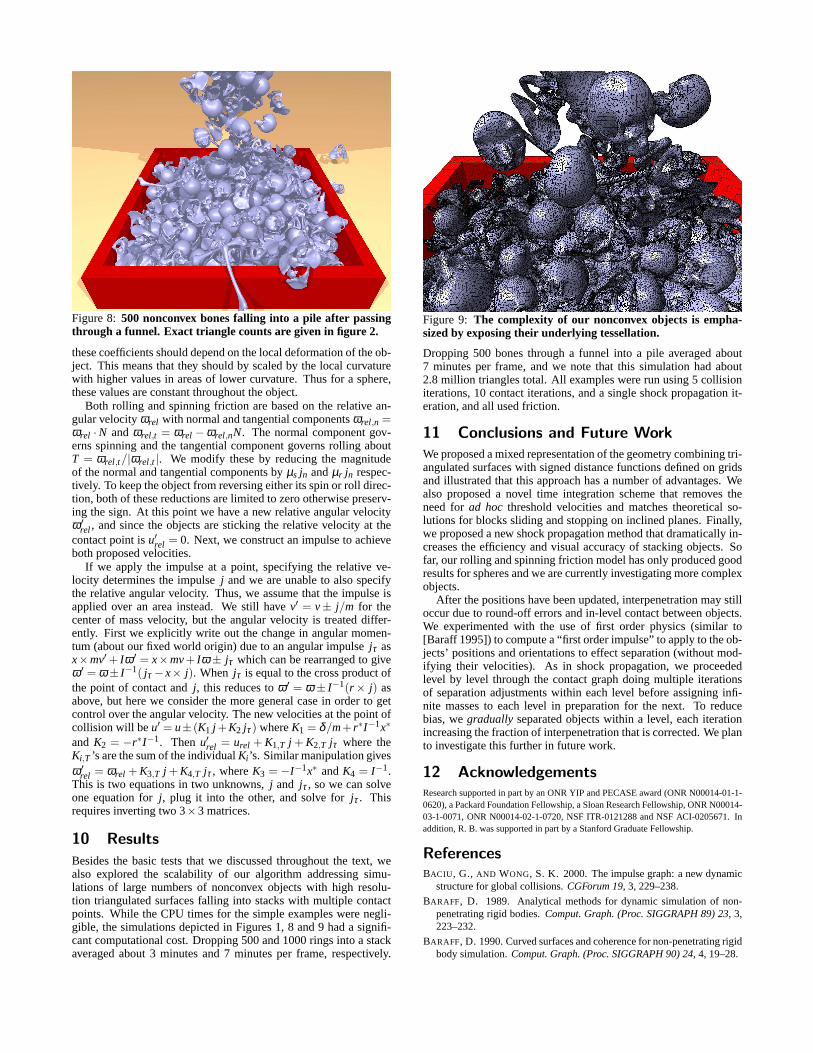
Figure 8: 500 nonconvex bones falling into a pile after passingthrough a funnel. Exact triangle counts are given in figure 2.

these coefficients should depend on the local deformation of the ob-ject. This means that they should by scaled by the local curvaturewith higher values in areas of lower curvature. Thus for a sphere,these values are constant throughout the object.

Both rolling and spinning friction are based on the relative an-gular velocityωrel with normal and tangential componentsωrel,n =ωrel ·N andωrel,t = ωrel −ωrel,nN. The normal component gov-erns spinning and the tangential component governs rolling aboutT = ωrel,t/|ωrel,t |. We modify these by reducing the magnitudeof the normal and tangential components byµs jn andµr jn respec-tively. To keep the object from reversing either its spin or roll direc-tion, both of these reductions are limited to zero otherwise preserv-ing the sign. At this point we have a new relative angular velocityω ′

rel , and since the objects are sticking the relative velocity at thecontact point isu′rel = 0. Next, we construct an impulse to achieveboth proposed velocities.

If we apply the impulse at a point, specifying the relative ve-locity determines the impulsej and we are unable to also specifythe relative angular velocity. Thus, we assume that the impulse isapplied over an area instead. We still havev′ = v± j/m for thecenter of mass velocity, but the angular velocity is treated differ-ently. First we explicitly write out the change in angular momen-tum (about our fixed world origin) due to an angular impulsejτ asx×mv′ + Iω ′ = x×mv + Iω ± jτ which can be rearranged to giveω ′ = ω ± I−1( jτ − x× j). When jτ is equal to the cross product ofthe point of contact andj, this reduces toω ′ = ω ± I−1(r× j) asabove, but here we consider the more general case in order to getcontrol over the angular velocity. The new velocities at the point ofcollision will beu′ = u± (K1 j +K2 jτ ) whereK1 = δ/m+ r∗I−1x∗

and K2 = −r∗I−1. Then u′rel = urel + K1,T j + K2,T jτ where theKi,T ’s are the sum of the individualKi’s. Similar manipulation givesω ′

rel = ωrel + K3,T j + K4,T jτ , whereK3 = −I−1x∗ andK4 = I−1.This is two equations in two unknowns,j and jτ , so we can solveone equation forj, plug it into the other, and solve forjτ . Thisrequires inverting two 3×3 matrices.

10 Results

Besides the basic tests that we discussed throughout the text, wealso explored the scalability of our algorithm addressing simu-lations of large numbers of nonconvex objects with high resolu-tion triangulated surfaces falling into stacks with multiple contactpoints. While the CPU times for the simple examples were negli-gible, the simulations depicted in Figures 1, 8 and 9 had a signifi-cant computational cost. Dropping 500 and 1000 rings into a stackaveraged about 3 minutes and 7 minutes per frame, respectively.

Figure 9: The complexity of our nonconvex objects is empha-sized by exposing their underlying tessellation.

Dropping 500 bones through a funnel into a pile averaged about7 minutes per frame, and we note that this simulation had about2.8 million triangles total. All examples were run using 5 collisioniterations, 10 contact iterations, and a single shock propagation it-eration, and all used friction.

11 Conclusions and Future Work

We proposed a mixed representation of the geometry combining tri-angulated surfaces with signed distance functions defined on gridsand illustrated that this approach has a number of advantages. Wealso proposed a novel time integration scheme that removes theneed forad hoc threshold velocities and matches theoretical so-lutions for blocks sliding and stopping on inclined planes. Finally,we proposed a new shock propagation method that dramatically in-creases the efficiency and visual accuracy of stacking objects. Sofar, our rolling and spinning friction model has only produced goodresults for spheres and we are currently investigating more complexobjects.

After the positions have been updated, interpenetration may stilloccur due to round-off errors and in-level contact between objects.We experimented with the use of first order physics (similar to[Baraff 1995]) to compute a “first order impulse” to apply to the ob-jects’ positions and orientations to effect separation (without mod-ifying their velocities). As in shock propagation, we proceededlevel by level through the contact graph doing multiple iterationsof separation adjustments within each level before assigning infi-nite masses to each level in preparation for the next. To reducebias, wegradually separated objects within a level, each iterationincreasing the fraction of interpenetration that is corrected. We planto investigate this further in future work.

12 Acknowledgements

Research supported in part by an ONR YIP and PECASE award (ONR N00014-01-1-0620), a Packard Foundation Fellowship, a Sloan Research Fellowship, ONR N00014-03-1-0071, ONR N00014-02-1-0720, NSF ITR-0121288 and NSF ACI-0205671. Inaddition, R. B. was supported in part by a Stanford Graduate Fellowship.

References

BACIU , G., AND WONG, S. K. 2000. The impulse graph: a new dynamicstructure for global collisions.CGForum 19, 3, 229–238.

BARAFF, D. 1989. Analytical methods for dynamic simulation of non-penetrating rigid bodies.Comput. Graph. (Proc. SIGGRAPH 89) 23, 3,223–232.

BARAFF, D. 1990. Curved surfaces and coherence for non-penetrating rigidbody simulation.Comput. Graph. (Proc. SIGGRAPH 90) 24, 4, 19–28.

BARAFF, D. 1991. Coping with friction for non-penetrating rigid bodysimulation.Comput. Graph. (Proc. SIGGRAPH 91) 25, 4, 31–40.

BARAFF, D. 1993. Issues in computing contact forces for non-penetratingrigid bodies.Algorithmica, 10, 292–352.

BARAFF, D. 1994. Fast contact force computation for nonpenetratingrigidbodies. InProc. SIGGRAPH 94, 23–34.

BARAFF, D. 1995. Interactive simulation of solid rigid bodies.IEEEComput. Graph. and Appl. 15, 3, 63–75.

BARZEL, R., HUGHES, J. F.,AND WOOD, D. N. 1996. Plausible motionsimulation for computer graphics. InComput. Anim. and Sim. ’96, Proc.Eurographics Workshop, 183–197.

BHATT, V., AND KOECHLING, J. 1995. Three-dimensional frictional rigid-body impact.ASME J. Appl. Mech. 62, 893–898.

BUSS, S. R. 2000. Accurate and efficient simulation of rigid-body rota-tions. J. Comput. Phys. 164, 2.

CHATTERJEE, A., AND RUINA , A. 1998. A new algebraic rigid bodycollision law based on impulse space considerations.ASME J. Appl.Mech. 65, 4, 939–951.

CHENNEY, S., AND FORSYTH, D. A. 2000. Sampling plausible solutionsto multi-body constraint problems. InProc. SIGGRAPH 2000, 219–228.

CUTLER, B., DORSEY, J., MCM ILLAN , L., MULLER, M., AND JAGNOW,R. 2002. A procedural approach to authoring solid models.ACM Trans.Graph. (SIGGRAPH Proc.) 21, 3, 302–311.

DESBRUN, M., AND GASCUEL, M.-P. 1995. Animating soft substanceswith implicit surfaces. InProc. SIGGRAPH 95, 287–290.

FISHER, S.,AND L IN , M. C. 2001. Deformed distance fields for simulationof non-penetrating flexible bodies. InComput. Anim. and Sim. ’01, Proc.Eurographics Workshop, 99–111.

FRISKEN, S. F., PERRY, R. N., ROCKWOOD, A. P., AND JONES, T. R.2000. Adaptively sampled distance fields: a general representation ofshape for computer graphics. InProc. SIGGRAPH 2000, 249–254.

GASCUEL, M.-P. 1993. An implicit formulation for precise contact mod-eling between flexible solids. InProc. SIGGRAPH 93, 313–320.

GIBSON, S. F. F. 1998. Using distance maps for accurate surface rep-resentation in sampled volumes. InProc. of IEEE Symp. on Vol. Vis.,23–30.

HAHN , J. K. 1988. Realistic animation of rigid bodies.Comput. Graph.(Proc. SIGGRAPH 88) 22, 4, 299–308.

HIROTA, G., FISHER, S., STATE, A., LEE, C., AND FUCHS, H. 2001. Animplicit finite element method for elastic solids in contact. InComput.Anim.

K IM , T.-Y., AND NEUMANN , U. 2002. Interactive multiresolution hairmodeling and editing.ACM Trans. Graph. (SIGGRAPH Proc.) 21, 3,620–629.

K IM , Y. J., OTADUY, M. A., L IN , M. C., AND MANOCHA, D. 2002. Fastpenetration depth computation for physically-based animation. In ACMSymp. Comp. Anim.

KOKKEVIS, E., METAXAS, D., AND BADLER, N. 1996. User-controlledphysics-based animation for articulated figures. InProc. Comput. Anim.’96.

LEWIS, A. D., AND MURRAY, R. M. 1995. Variational principles inconstrained systems: theory and experiments.Int. J. Nonlinear Mech.30, 6, 793–815.

L IN , M., AND GOTTSCHALK, S. 1998. Collision detection between geo-metric models: A survey. InProc. of IMA Conf. on Math. of Surfaces,37–56.

M ILENKOVIC , V. J.,AND SCHMIDL , H. 2001. Optimization-based anima-tion. In Proc. SIGGRAPH 2001, 37–46.

M ILENKOVIC , V. J. 1996. Position-based physics: simulating the motionof many highly interacting spheres and polyhedra. InProc. SIGGRAPH96, 129–136.

M IRTICH, B., AND CANNY, J. 1995. Impulse-based dynamic simula-tion. In Alg. Found. of Robotics, A. K. Peters, Boston, MA, K. Goldberg,D. Halperin, J.-C. Latombe, and R. Wilson, Eds., 407–418.

M IRTICH, B., AND CANNY, J. 1995. Impulse-based simulation of rigid

bodies. InProc. of 1995 Symp. on Int. 3D Graph., 181–188, 217.

M IRTICH, B. 1996. Fast and accurate computation of polyhedral massproperties.J. Graph. Tools 1, 2, 31–50.

M IRTICH, B. 2000. Timewarp rigid body simulation. InProc. SIGGRAPH2000, 193–200.

MOORE, M., AND WILHELMS , J. 1988. Collision detection and responsefor computer animation.Comput. Graph. (Proc. SIGGRAPH 88) 22, 4,289–298.

MUSETH, K., BREEN, D., WHITAKER , R., AND BARR, A. 2002. Levelset surface editing operators.ACM Trans. Graph. (SIGGRAPH Proc.)21, 3, 330–338.

OSHER, S., AND FEDKIW, R. 2002. Level Set Methods and DynamicImplicit Surfaces. Springer-Verlag. New York, NY.

PANDOLFI , A., KANE, C., MARSDEN, J., AND ORTIZ, M. 2002. Time-discretized variational formulation of non-smooth frictional contact.Int.J. Num. Meth. in Eng. 53, 1801–1829.

PENTLAND , A., AND WILLIAMS , J. 1989. Good vibrations: modal dy-namics for graphics and animation.Comput. Graph. (Proc. SIGGRAPH89) 23, 3, 215–222.

PONAMGI , M. K., MANOCHA, D., AND L IN , M. C. 1995. Incrementalalgorithms for collision detection between solid models. InProc. ACMSymp. Solid Model. and Appl., 293–304.

POPOVIC, J., SEITZ, S. M., ERDMANN , M., POPOVIC, Z., AND WITKIN ,A. 2000. Interactive manipulation of rigid body simulations.In Proc.SIGGRAPH 2000, 209–217.

REDON, S., KHEDDAR, A., AND COQUILLART, S. 2002. Fast continuouscollision detection between rigid bodies.CGForum 21, 3, 279–288.

SAUER, J.,AND SCHOMER, E. 1998. A constraint-based approach to rigidbody dynamics for virtual reality applications. InProc. ACM Symp. onVirt. Reality Soft. and Tech., 153–162.

SCHMIDL , H. 2002.Optimization-based animation. PhD thesis, Universityof Miami.

SCHROEDER, W. J., LORENSEN, W. E., AND L INTHICUM , S. 1994. Im-plicit modeling of swept surfaces and volumes. InProc. of Vis., IEEEComputer Society Press, 40–55.

SCLAROFF, S.,AND PENTLAND , A. 1991. Generalized implicit functionsfor computer graphics.Comput. Graph. (Proc. SIGGRAPH 91) 25, 4,247–250.

SETHIAN , J. 1996. A fast marching level set method for monotonicallyadvancing fronts.Proc. Natl. Acad. Sci. 93, 1591–1595.

SIMS, K. 1994. Evolving virtual creatures. InProc. SIGGRAPH 94, 15–22.

STEWART, D. E., AND TRINKLE , J. C. 2000. An implicit time-steppingscheme for rigid body dynamics with coulomb friction. InIEEE Int.Conf. on Robotics and Automation, 162–169.

STEWART, D. E. 2000. Rigid-body dynamics with friction and impact.SIAM Review 42, 1, 3–39.

TERZOPOULOS, D., PLATT, J., BARR, A., AND FLEISCHER, K. 1987.Elastically deformable models.Comput. Graph. (Proc. SIGGRAPH 87)21, 4, 205–214.

TSITSIKLIS, J. 1995. Efficient algorithms for globally optimal trajectories.IEEE Trans. on Automatic Control 40, 1528–1538.

WEBB, R., AND GIGANTE, M. 1992. Using dynamic bounding volumehierarchies to improve efficiency of rigid body simulations. In Comm.with Virt. Worlds, CGI Proc. 1992, 825–841.

WESTERMANN, R., KOBBELT, L., AND ERTL, T. 1999. Real-time explo-ration of regular volume data by adaptive reconstruction of isosurfaces.The Vis. Comput. 15, 2, 100–111.