NonEquilibrium Thermodynamics of Flowing Systems: 1

Antony N. Beris

Multiscale Modeling and Simulation of Complex FluidsCenter for Scientific Computing and Mathematical Modeling

University of Maryland, College Park

Schedule:

1. 4/13/07, 9:30 am Introduction. One mode viscoelasticity.2. 4/13/07, 10:15 am Coupled transport: Two-fluid model.3. 4/14/07, 2:00 pm Modeling under constraints: Liquid crystals.4. 4/14/07, 3:00 am Non-homogeneous systems: Surface effects.

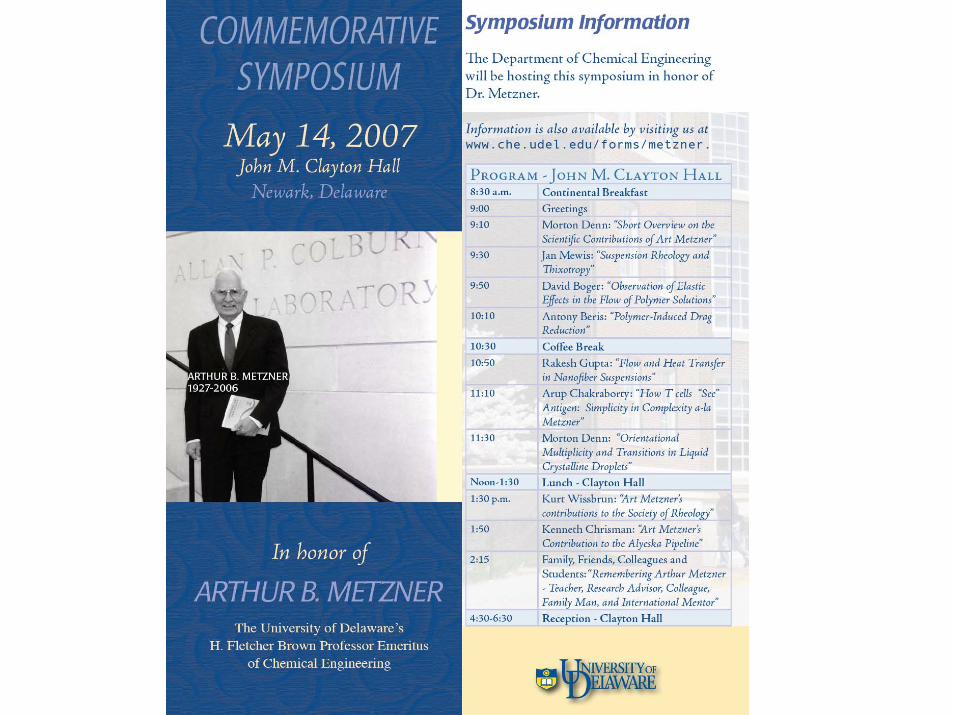
Art Metzner, 04/13/1927 – 05/02/2006Commemorative Symposium: May 14, 2007, Dept. of Chem. Engrg., Univ. of Delaware

Motivation

• To use a framework that it allows the imposition “ab initio” of the most restrictive physically possible guidelines governing the dynamics of complex systems

• Certain limitations are inevitable: most importantly, that the system we study is “close enough” to equilibrium; yet we want the formalism to not be introducing arbitrary constraints. Here we also limit ourselves to macroscopic descriptions.

General Features

• The general formalism has to reduce to well-established ones at characteristic limiting cases:– In the limit of infinite time: Equilibrium (Gibbs)

thermodynamics– In the limit of reversible dynamics: Hamiltonian

dynamics– In the limit of infinitesimally small deviations from

equilibrium: Linear Irreversible Thermodynamics (Onsager relations)

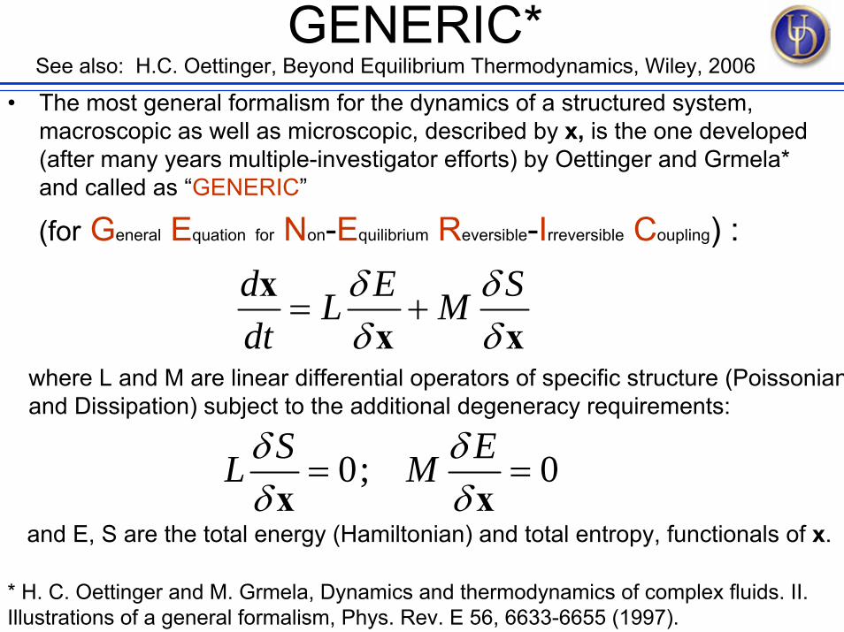
GENERIC*• The most general formalism for the dynamics of a structured system,

macroscopic as well as microscopic, described by x, is the one developed (after many years multiple-investigator efforts) by Oettinger and Grmela* and called as “GENERIC”

(for General Equation for Non-Equilibrium Reversible-Irreversible Coupling) :

d E SL Mdt

δ δδ δ

= +x

x xwhere L and M are linear differential operators of specific structure (Poissonianand Dissipation) subject to the additional degeneracy requirements:

0; 0S EL Mδ δδ δ

= =x x

and E, S are the total energy (Hamiltonian) and total entropy, functionals of x.

See also: H.C. Oettinger, Beyond Equilibrium Thermodynamics, Wiley, 2006

* H. C. Oettinger and M. Grmela, Dynamics and thermodynamics of complex fluids. II.Illustrations of a general formalism, Phys. Rev. E 56, 6633-6655 (1997).

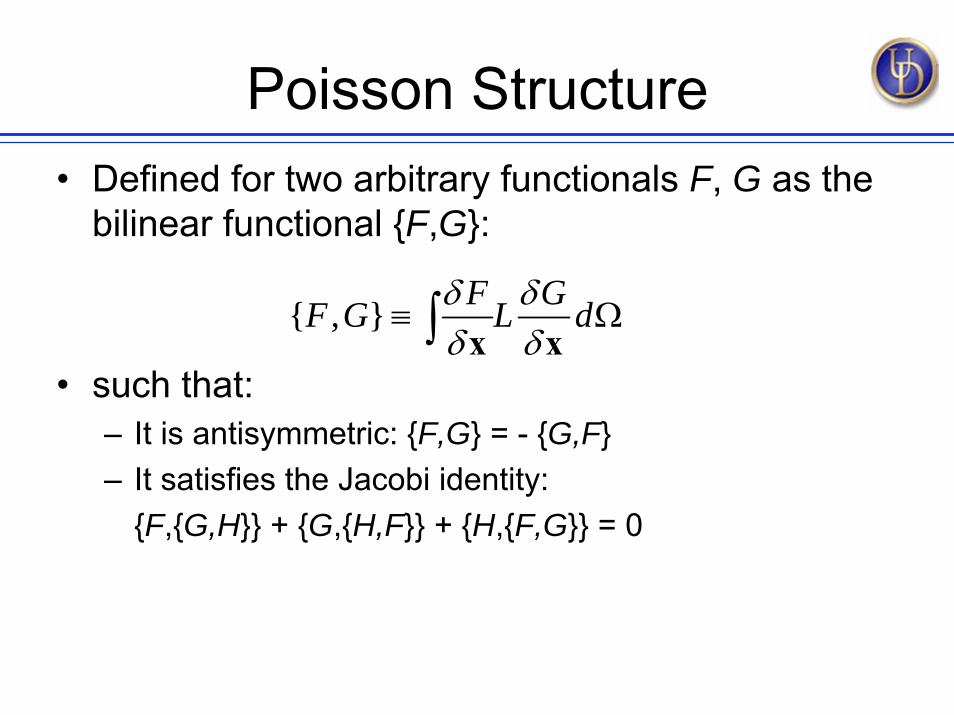
Poisson Structure• Defined for two arbitrary functionals F, G as the

bilinear functional F,G:

• such that:– It is antisymmetric: F,G = - G,F– It satisfies the Jacobi identity:

F,G,H + G,H,F + H,F,G = 0

, F GF G L dδ δδ δ

≡ Ω∫ x x

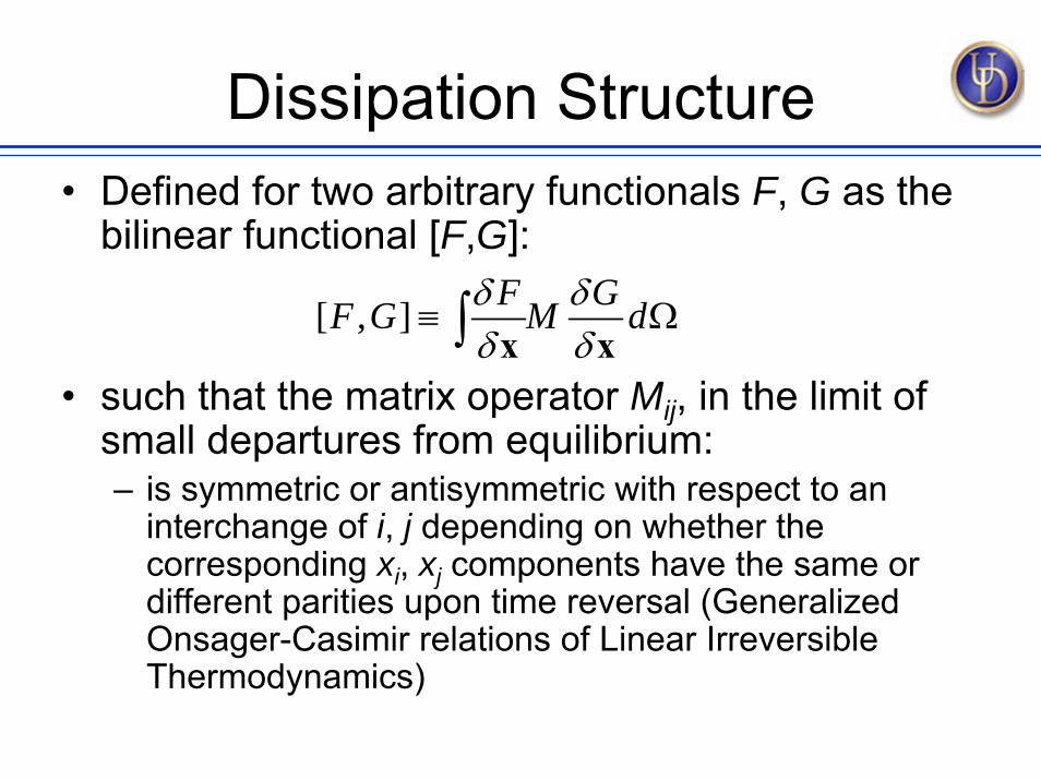
Dissipation Structure• Defined for two arbitrary functionals F, G as the

bilinear functional [F,G]:

• such that the matrix operator Mij, in the limit of small departures from equilibrium:– is symmetric or antisymmetric with respect to an

interchange of i, j depending on whether the corresponding xi, xj components have the same or different parities upon time reversal (Generalized Onsager-Casimir relations of Linear Irreversible Thermodynamics)

[ , ] F GF G M dδ δδ δ

≡ Ω∫ x x

Features of GENERIC• It can be shown to be consistent with all well

accepted dynamic transport equations ranging from the very microscopic (Maxwell-Boltzmann) to the microscopic (kinetic theory in polymers) and macroscopic (transport phenomena) levels

• It can provide corrections/suggestions to many complex modeling problems, such as:– Reptation theory models– Closure approximations

see Öttinger’s homepage: http://www.polyphys.mat.ethz.ch/ andÖttinger H-C, Beyond Equilibrium Thermodynamics, Wiley 2005

Single Generaror Approximation

• For macroscopic systems, it is possible to deduce a simpler structure based on the local equilibrium approximation according to which there is a local system entropy density that can alternatively to the energy be used to characterize the system– the entropy and energy potentials are directly related– we can express the dynamics solely in terms of energy

(Hamiltonian) potentials

• This is shown to be equivalent to GENERIC:– Edwards BJ, J. Non-Equil. Thermodyn., 23:300-332 (1998)

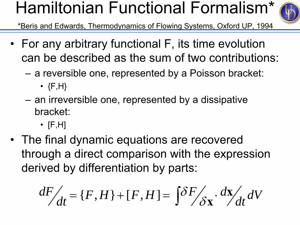
Hamiltonian Functional Formalism**Beris and Edwards, Thermodynamics of Flowing Systems, Oxford UP, 1994

• For any arbitrary functional F, its time evolution can be described as the sum of two contributions:– a reversible one, represented by a Poisson bracket:

• F,H

– an irreversible one, represented by a dissipative bracket:

• [F,H]

• The final dynamic equations are recovered through a direct comparison with the expression derived by differentiation by parts:

, [ , ]dF F dF H F H dVdt dtδ

δ= + = ⋅∫ xx

Advantages of Hamiltonian Formalism (1)

• It only requires knowledge of the following:– A set of macroscopic variables, taken uniformly as volume

densities. The include, in addition to the equilibrium thermodynamic ones (the component mass density, ρi, for every component i, the entropy density si), the momentum density, ρv, and any additional structural parameter, again expressed as a density

– The total energy of the system or any suitable Lagrange transform of it, typically the total Helmholtz free energy, expressed as a functional of all other densities with the temperature substituting for the entropy density

– The Poisson bracket, F,H– The dissipation bracket, [F,H]

Advantages of Hamiltonian Formalism (2)

A set of macroscopic variables can easily be assumed depending on the physics that we want to incorporate to the problemThe total Helmholtz free energy can also easily be constructed as the sum of kinetic energy plus an extended thermodynamic free energy that typically includes an easily derived expression (in terms of the structural parameters) in addition to a standard equilibrium expressionThe Poisson bracket, F,H is rarely needed by itself: only when an equation is put together for the first time characteristic of the variables involved in this system; otherwise, its effect is probably already known from previous work: it corresponds to a standard reversible dynamics. For viscoelastic flows, this corresponds to the terms defining an upper convected derivativeThe dissipation bracket, [F,H] is the only one to contain major new information and is typically where our maximum ignorance lies. Barren any other information (say, by comparison against a microscopic theory) the main information that we can use is a linear irreversible thermodynamics expression: according to that, the dissipation bracket becomes a bilinear functional in terms of all the nonequilibrium Hamiltonian gradients with an additional nonlinear (in H) correction with respect to δF/δs (entropy correction) that can be easily calculated so that the conservation of the total energy is satisfied: [H,H] = 0.

Example Case: Single Mode Viscoelasticity

• Reference (available in electronic form from beris@che.udel.edu):– A.N. Beris, Simple Nonequilibrium

Thermodynamics Applications to Polymer Rheology (As it appeared on: RHEOLOGY REVIEWS 2003, The British Society of Rheology(publisher), 37-75)

Variables• For an incompressible, homogeneous (uniform

polymer concentration, n=chain number density is constant) system we have– v, the velocity– s, the entropy density (alternatively, T, temperature)– c, the conformation tensor where

• C = <RR> (second moment of the end-to-end distribution function) = nc

• At equilibrium, c=kBT/K where K is the equilibrium equivalent entropic elastic energy constant of the polymer chain

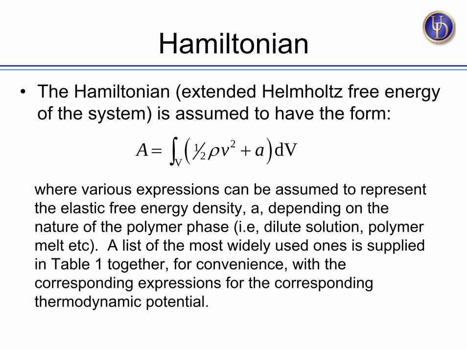
Hamiltonian• The Hamiltonian (extended Helmholtz free energy

of the system) is assumed to have the form:

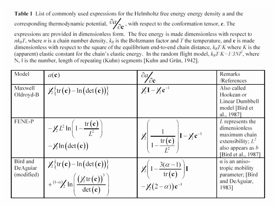
( )212V

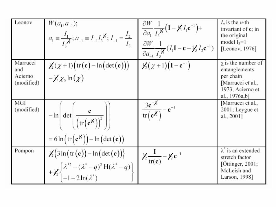
dVA v aρ= +∫where various expressions can be assumed to represent the elastic free energy density, a, depending on the nature of the polymer phase (i.e, dilute solution, polymer melt etc). A list of the most widely used ones is supplied in Table 1 together, for convenience, with the corresponding expressions for the corresponding thermodynamic potential.

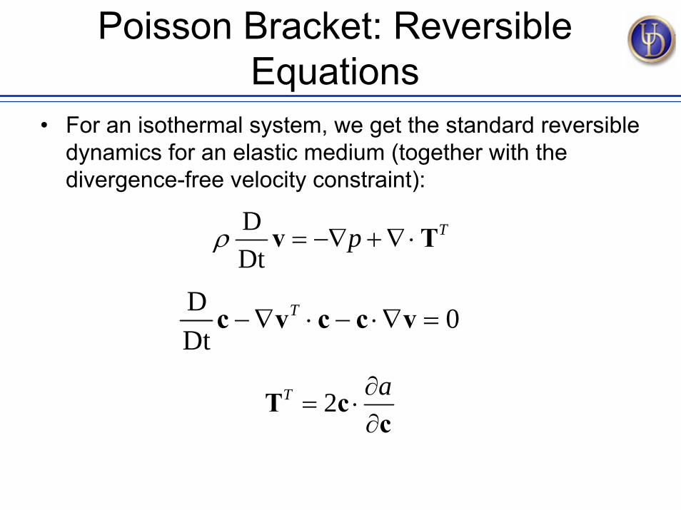
Poisson Bracket: Reversible Equations

• For an isothermal system, we get the standard reversible dynamics for an elastic medium (together with the divergence-free velocity constraint):

DDt

Tpρ = −∇ +∇⋅v T

D 0Dt

T−∇ ⋅ − ⋅∇ =c v c c v

2T a∂= ⋅

∂T c

c

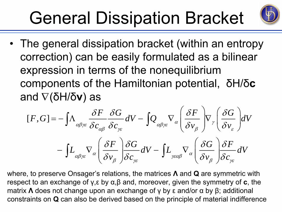
General Dissipation Bracket• The general dissipation bracket (within an entropy

correction) can be easily formulated as a bilinear expression in terms of the nonequilibriumcomponents of the Hamiltonian potential, δH/δcand ∇(δH/δv) as

[ , ] F G F GF G dV Q dVc c v v

F G G FL dV L dVv c v c

α γαβγε αβγεαβ γε β ε

α ααβγε γεαββ γε β γε

δ δ δ δδ δ δ δ

δ δ δ δδ δ δ δ

⎛ ⎞ ⎛ ⎞= − Λ − ∇ ∇⎜ ⎟ ⎜ ⎟⎜ ⎟ ⎝ ⎠⎝ ⎠

⎛ ⎞ ⎛ ⎞− ∇ − ∇⎜ ⎟ ⎜ ⎟⎜ ⎟ ⎜ ⎟

⎝ ⎠ ⎝ ⎠

∫ ∫

∫ ∫where, to preserve Onsager’s relations, the matrices Λ and Q are symmetric with respect to an exchange of γ,ε by α,β and, moreover, given the symmetry of c, the matrix Λ does not change upon an exchange of γ by ε and/or α by β; additional constraints on Q can also be derived based on the principle of material indifference

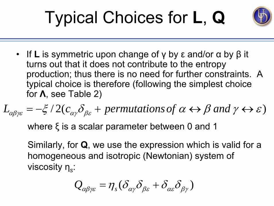
Typical Choices for L, Q

• If L is symmetric upon change of γ by ε and/or α by β it turns out that it does not contribute to the entropy production; thus there is no need for further constraints. A typical choice is therefore (following the simplest choice for Λ, see Table 2)

/ 2( )L c permutationsof andαβγε αγ βεξ δ α β γ ε= − + ↔ ↔where ξ is a scalar parameter between 0 and 1

Similarly, for Q, we use the expression which is valid for a homogeneous and isotropic (Newtonian) system of viscosity ηs:

( )sQαβγε αγ βε αε βγη δ δ δ δ= +

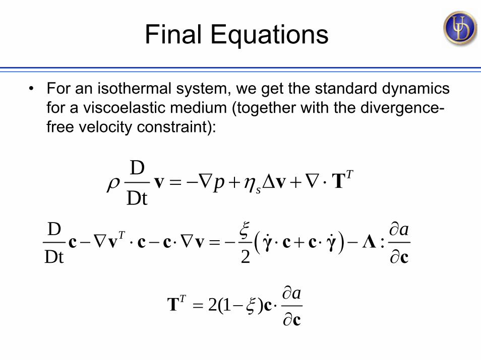
Final Equations

• For an isothermal system, we get the standard dynamics for a viscoelastic medium (together with the divergence-free velocity constraint):

DDt

Tspρ η= −∇ + ∆ +∇⋅v v T

( )D :Dt 2

T aξ ∂−∇ ⋅ − ⋅∇ = − ⋅ + ⋅ −

∂c v c c v γ c c γ Λ

c

2(1 )T aξ ∂= − ⋅

∂T c

c

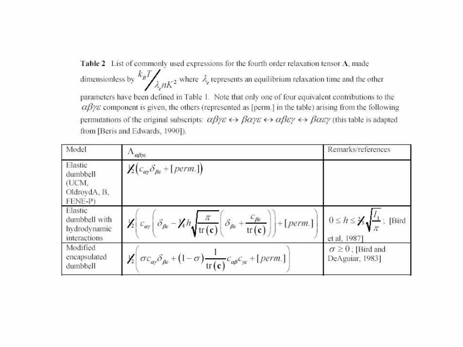
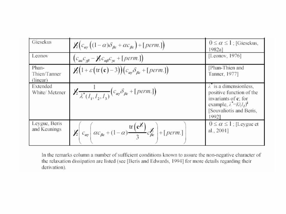
Typical Choices for Λ

• Various models can be generated using different expressions for the relaxation tensor Λ.

• A compilation of some of the most often employed forms can be found in Table 2

Conclusions• The Hamiltonian formalism can provide a uniform

representation for viscoelastic models• New possibilities thus arise for new model

development through “mix and match” of terms• In addition, the evaluation of thermodynamic

consistency is facilitated: new constraints can be easily derived on acceptable parameter values and suitable approximations for the dissipative terms of the equations

• The extension of the above-mentioned work to multimode models is straightforward! See the mentioned references (book and review) for several characteristic examples