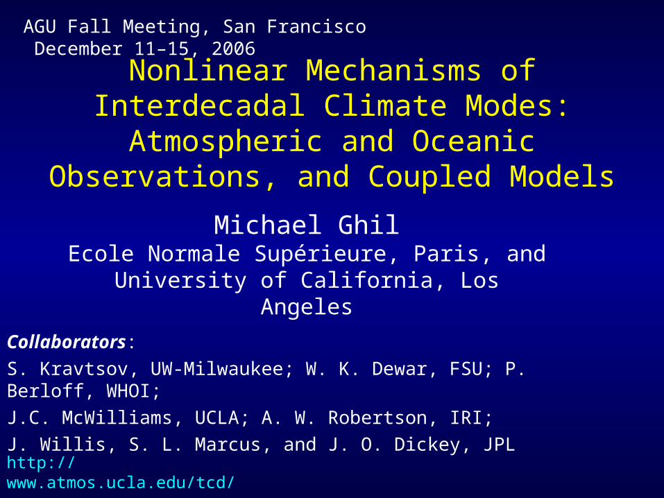
Nonlinear Mechanisms of Interdecadal Climate Modes: Atmospheric and Oceanic

Observations, and Coupled Models

Michael GhilEcole Normale Supérieure, Paris, andUniversity of California, Los Angeles

Collaborators:

S. Kravtsov, UW-Milwaukee; W. K. Dewar, FSU; P. Berloff, WHOI;

J.C. McWilliams, UCLA; A. W. Robertson, IRI;

J. Willis, S. L. Marcus, and J. O. Dickey, JPL

AGU Fall Meeting, San Francisco December 11–15, 2006

http://www.atmos.ucla.edu/tcd/

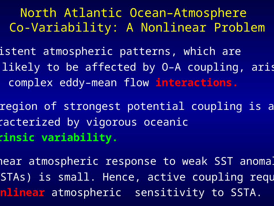
North Atlantic Ocean–Atmosphere Co-Variability: A Nonlinear Problem

• Persistent atmospheric patterns, which are

most likely to be affected by O–A coupling, arise

from complex eddy–mean flow interactions.

• The region of strongest potential coupling is also

characterized by vigorous oceanic

intrinsic variability.

• Linear atmospheric response to weak SST anomalies

(SSTAs) is small. Hence, active coupling requires

nonlinear atmospheric sensitivity to SSTA.

Observational Analyses• NCEP/NCAR Reanalysis (Kalnay et al., 1996)

zonally averaged zonal wind data set:

58 Northern Hemisphere winters

[100N–700N] and (Dec.–March)

• Sea-surface temperature (SST)

observations (annual means, same period)

• Upper ocean heat content (OHC) data (detrended,

1965–2006) (Levitus et al., 2005; Lyman et al., 2006)

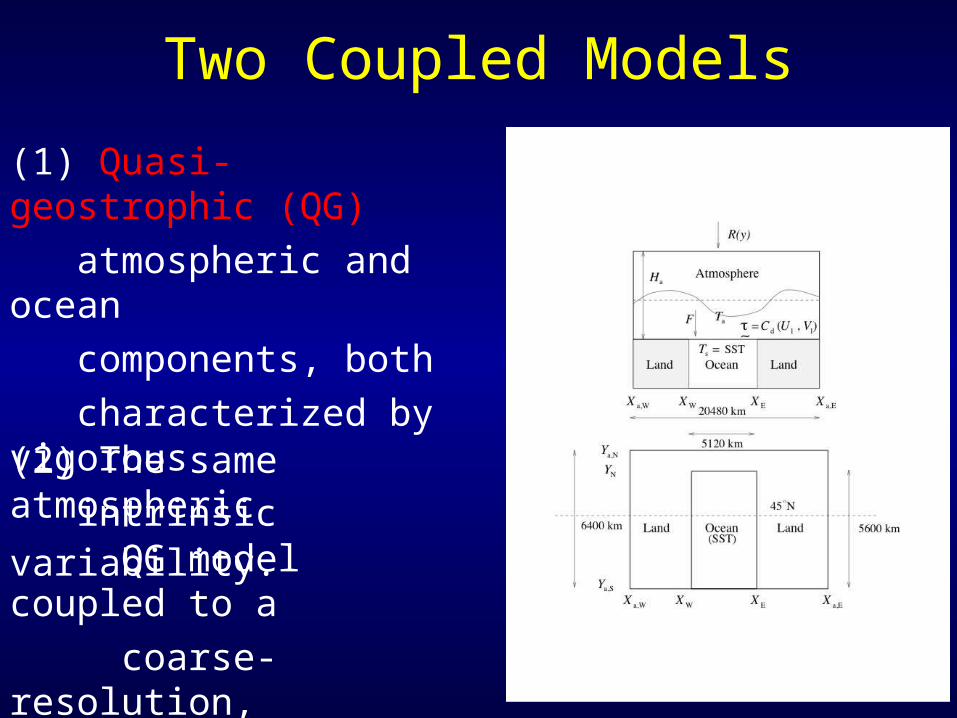
Two Coupled Models

(1) Quasi-geostrophic (QG)

atmospheric and ocean

components, both

characterized by vigorous

intrinsic variability.

(2) The same atmospheric

QG model coupled to a

coarse-resolution,

primitive-equation (PE)

ocean (called OPE).

Methodology

• Study nonlinear aspects of intrinsic atmospheric

variability by identifying anomalously persistent

patterns (time scales longer than about a week).

• Identify long-term (decadal and longer) changes

in the frequency of occurrence of such states.

• Connect the latter changes with the changes

in boundary forcing (e.g., SST anomalies), as well

as with the upper-ocean’s (inter-)decadal variability.

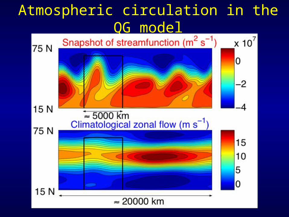
Atmospheric circulation in the QG model

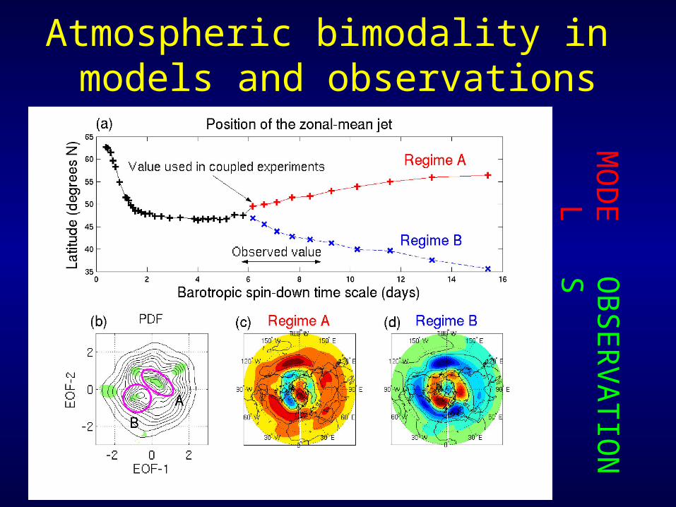
Atmospheric bimodality in models and observationsM

OD

ELO

BS

ER

VA

TIO

NS

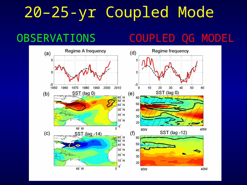
20–25-yr Coupled Mode

OBSERVATIONS COUPLED QG MODEL

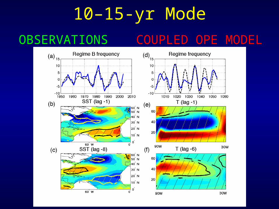
10–15-yr Mode

OBSERVATIONS COUPLED OPE MODEL

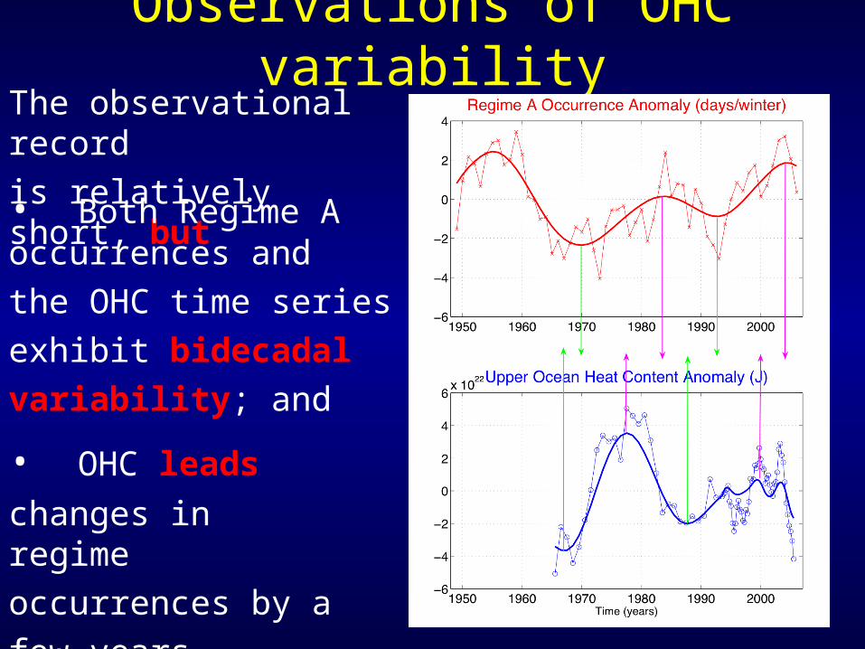
Observations of OHC variabilityThe observational record

is relatively short, but

• Both Regime A occurrences and

the OHC time series

exhibit bidecadal

variability; and

• OHC leads

changes in regime

occurrences by a

few years.

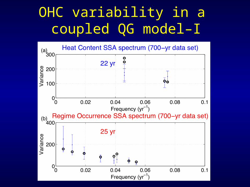
OHC variability in a coupled QG model–I

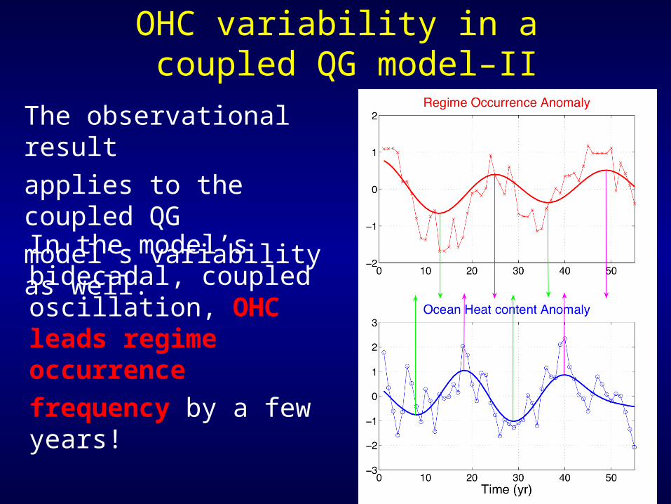
OHC variability in a coupled QG model–II

The observational result

applies to the coupled QG

model’s variability as well:

In the model’s bidecadal, coupled oscillation, OHC leads regime occurrence

frequency by a few years!

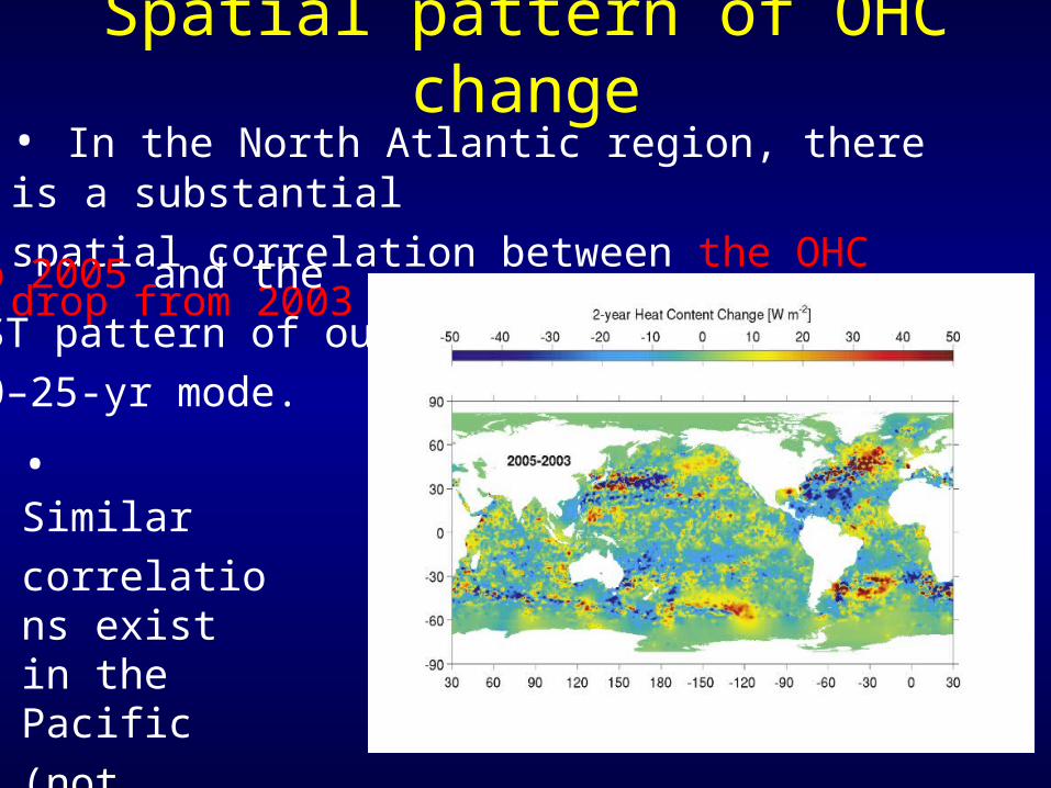
Spatial pattern of OHC change• In the North Atlantic region, there is a substantial

spatial correlation between the OHC drop from 2003

to 2005 and the

SST pattern of our

20–25-yr mode.

• Similar

correlations exist in the Pacific

(not shown).

Summary

• The bimodal character of atmospheric LFV is the

amplifier of atmospheric sensitivity to SSTAs.

• Evidence is mounting for decadal and bidecadal

coupled climate signals, whose centers of action

lie in the North Atlantic Ocean.

• Signatures of these signals are found in the NH

zonal wind and SST data, as well as in global

upper-ocean heat content (OHC) data.

• Intermediate coupled models exhibit oscillations

that correctly reproduce the observed time scales

and phase relations between key climate variables.

Selected referencesDijkstra, H. A., & M. Ghil, 2005: Low-frequency variability of the large-scale ocean

circulation: A dynamical systems approach, Rev. Geophys., 43, RG3002, doi:10.1029/2002RG000122.

Feliks, Y., M. Ghil, and E. Simonnet, 2007: Low-frequency variability in the mid-latitude baroclinic atmosphere induced by an oceanic thermal front, J. Atmos. Sci., 64(1), 97–116.

Kravtsov, S., A. W. Robertson, & M. Ghil, 2005: Bimodal behavior in the zonal mean flow of a baroclinic beta-channel model, J. Atmos. Sci., 62, 1746–1769

Kravtsov, S., A. W. Robertson, & M. Ghil, 2006: Multiple regimes and low-frequency oscillations in the Northern Hemisphere's zonal-mean flow, J. Atmos. Sci., 63 (3), 840–860.

Kravtsov, S., P. Berloff, W. K. Dewar, M. Ghil, & J. C. McWilliams, 2006: Dynamical origin of low-frequency variability in a highly nonlinear mid-latitude coupled model. J. Climate, accepted.

Kravtsov, S., W. K. Dewar, P. Berloff, J. C. McWilliams, & M. Ghil, 2006: A highly nonlinear coupled mode of decadal variability in a mid-latitude ocean–atmosphere model. Dyn. Atmos. Oceans, accepted.

Lyman J. M., J. K. Willis, & G. C. Johnson, 2006: Recent cooling of the upper ocean, Geophys. Res. Lett., 33 (18): Art. No. L18604.

.

http://www.atmos.ucla.edu/tcd/