Embed Size (px)
Citation preview
Orbital Stabilization of Underactuated
Nonlinear Systems.∗
Anton Shiriaev† and Carlos Canudas-de-Wit‡ †‡
November 24, 2003
∗This presentation is based on [10] and [7]†† Department of Applied Physics and Electronics, University of Umea, SE-901 87
Umea, SWEDEN. Email: [email protected]‡‡ Laboratoire d’Automatique de Grenoble, UMR CNRS 5528, ENSIEG-INPG,
B.P. 46, 38 402, ST. Martin d´Heres, FRANCE. Email: carlos.canudas-de-wit@
inpg.fr.
0-0
Virtual Constraints a Constructive Tool For Orbital Stabilization. Slide # 1
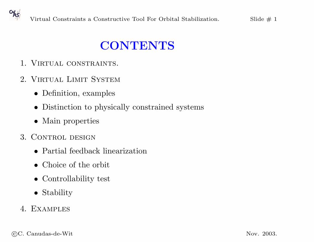
CONTENTS
1. Virtual constraints.
2. Virtual Limit System
• Definition, examples• Distinction to physically constrained systems• Main properties
3. Control design
• Partial feedback linearization• Choice of the orbit• Controllability test• Stability
4. Examples
c©C. Canudas-de-Wit Nov. 2003.
Virtual Constraints a Constructive Tool For Orbital Stabilization. Slide # 2
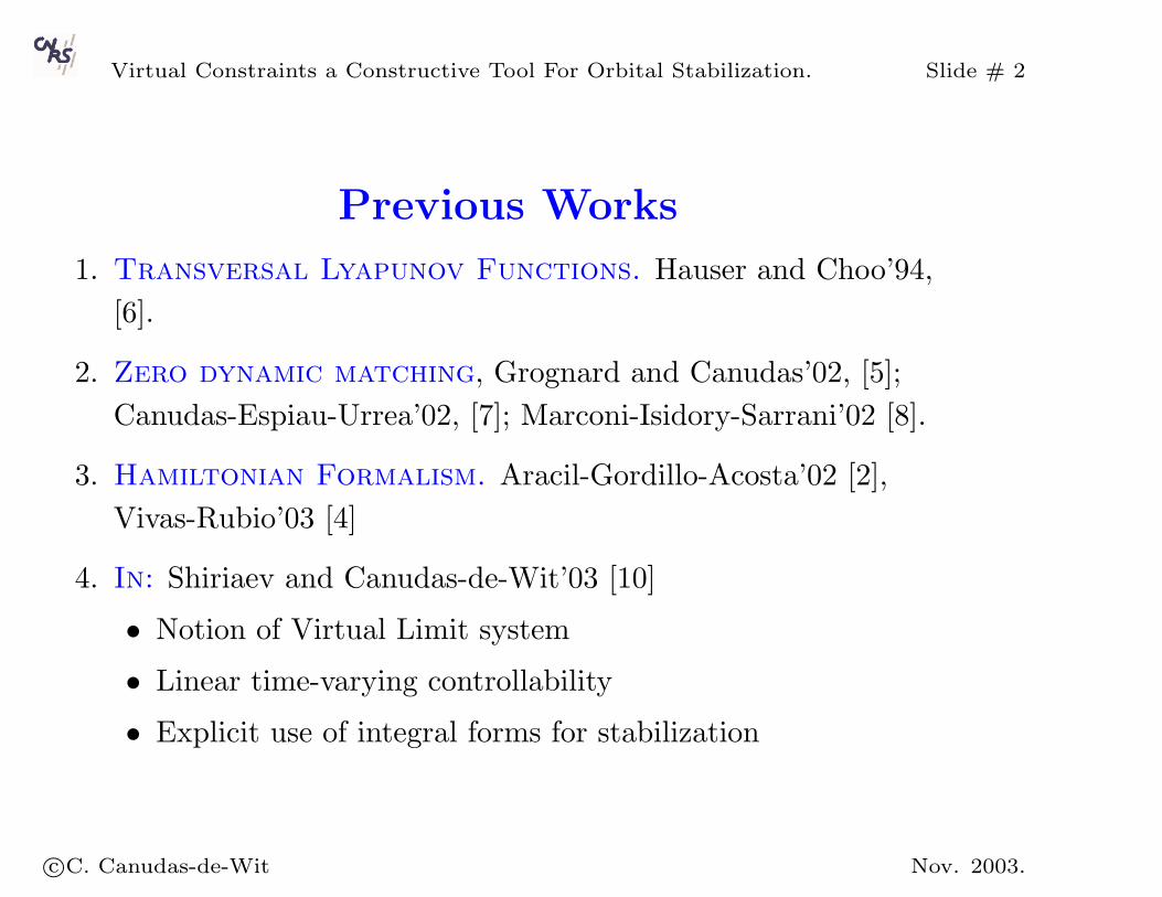
Previous Works
1. Transversal Lyapunov Functions. Hauser and Choo’94,[6].
2. Zero dynamic matching, Grognard and Canudas’02, [5];Canudas-Espiau-Urrea’02, [7]; Marconi-Isidory-Sarrani’02 [8].
3. Hamiltonian Formalism. Aracil-Gordillo-Acosta’02 [2],Vivas-Rubio’03 [4]
4. In: Shiriaev and Canudas-de-Wit’03 [10]
• Notion of Virtual Limit system• Linear time-varying controllability• Explicit use of integral forms for stabilization
c©C. Canudas-de-Wit Nov. 2003.
Virtual Constraints a Constructive Tool For Orbital Stabilization. Slide # 3
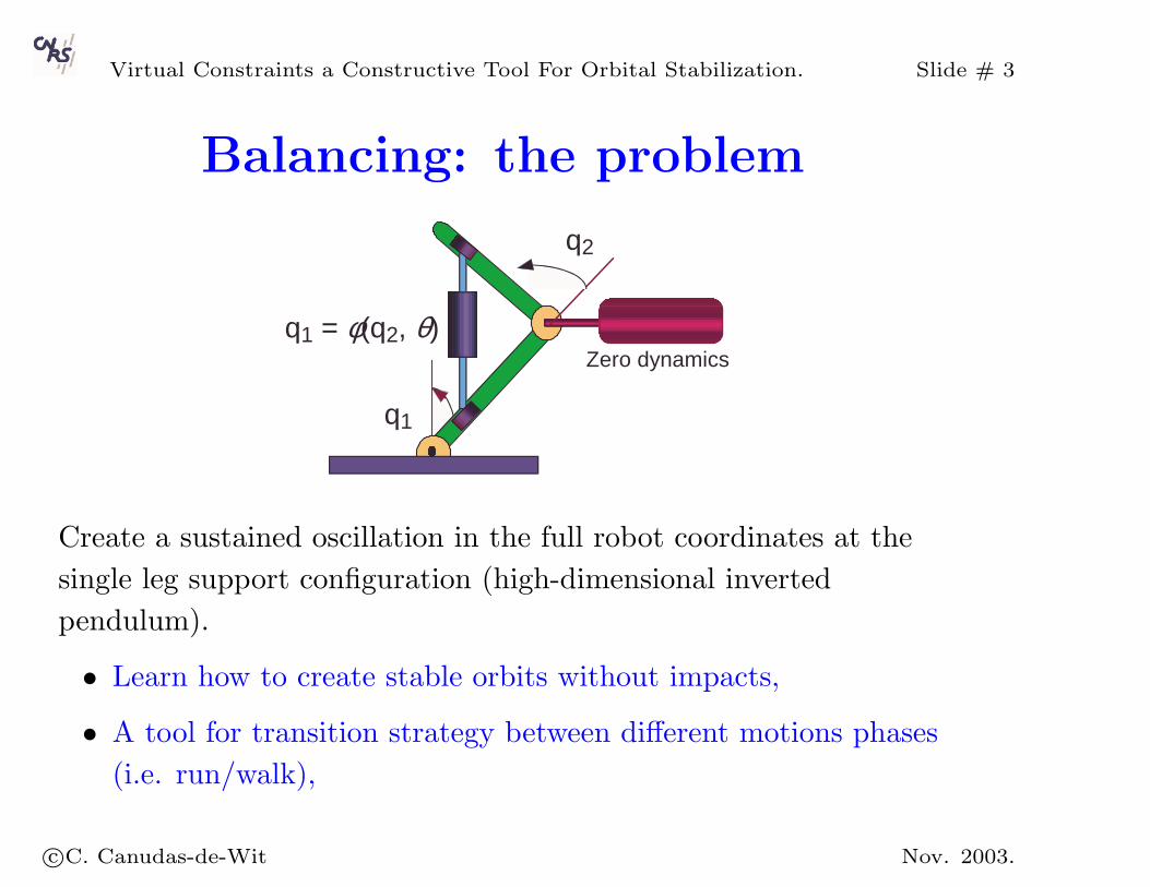
Balancing: the problem
Zero dynamics
q2
q1
q1 = φ(q2, θ)
Create a sustained oscillation in the full robot coordinates at thesingle leg support configuration (high-dimensional invertedpendulum).
• Learn how to create stable orbits without impacts,• A tool for transition strategy between different motions phases(i.e. run/walk),
c©C. Canudas-de-Wit Nov. 2003.
Virtual Constraints a Constructive Tool For Orbital Stabilization. Slide # 4
Key steps
We consider underactuated Lagrangian systems
d
dt
(∂L∂q
)− ∂L
∂q= B(q)u
with a degree of underactuation equal to one.
• n − 1 virtual constraint ϕ(q, p) = 0, with p, being parametervector.
• The virtually constrained system has the form
α(θ, p)θ + β(θ, p)θ2 + γ(θ, p) = 0
which posses a conserved quantity I = I(θ, θ, θ(0), θ(0), p)
• Characterize the LTV controllability.• Construct a (local) stabilizable control law.
c©C. Canudas-de-Wit Nov. 2003.
Virtual Constraints a Constructive Tool For Orbital Stabilization. Slide # 5
Balancing vs Walking:What changes ?
Conceptual differences:
• Motion without impacts, then• Cycles should be stabilized dynamically.• “Passive” stable cycles do not exist.
Two possible methods:
• Matching a desired limit cycle exo-system,• Use the trajectory controllability of the target cycle.
c©C. Canudas-de-Wit Nov. 2003.
Virtual Constraints a Constructive Tool For Orbital Stabilization. Slide # 6
The matching solution
The parameter p(t) may be time-varying i.e.
y = h0(q)− hd(θ(q), p(t))
Find hd(θ(q), p(t)) and an adaptation law (dynamic feedback) for p,such that:
the zero dynamics
x1 = x2
x2 = β(x, hd, p(t), p(t), p(t))
exhibits stable periodic behaviour, with stable solutions for p(t).
c©C. Canudas-de-Wit Nov. 2003.
Virtual Constraints a Constructive Tool For Orbital Stabilization. Slide # 7
• Target orbit (exosystem) defines a target orbit Ωd(x)defines a closed path in the plane.
x1 = x2
x2 = βd(x)
• Dynamic Matching condition. Solve for p, to satisfy
β(x, hd, p, p, p) = βd(x)
while ensuring boundedness of the obtained solutions for p(t).
c©C. Canudas-de-Wit Nov. 2003.
Virtual Constraints a Constructive Tool For Orbital Stabilization. Slide # 8
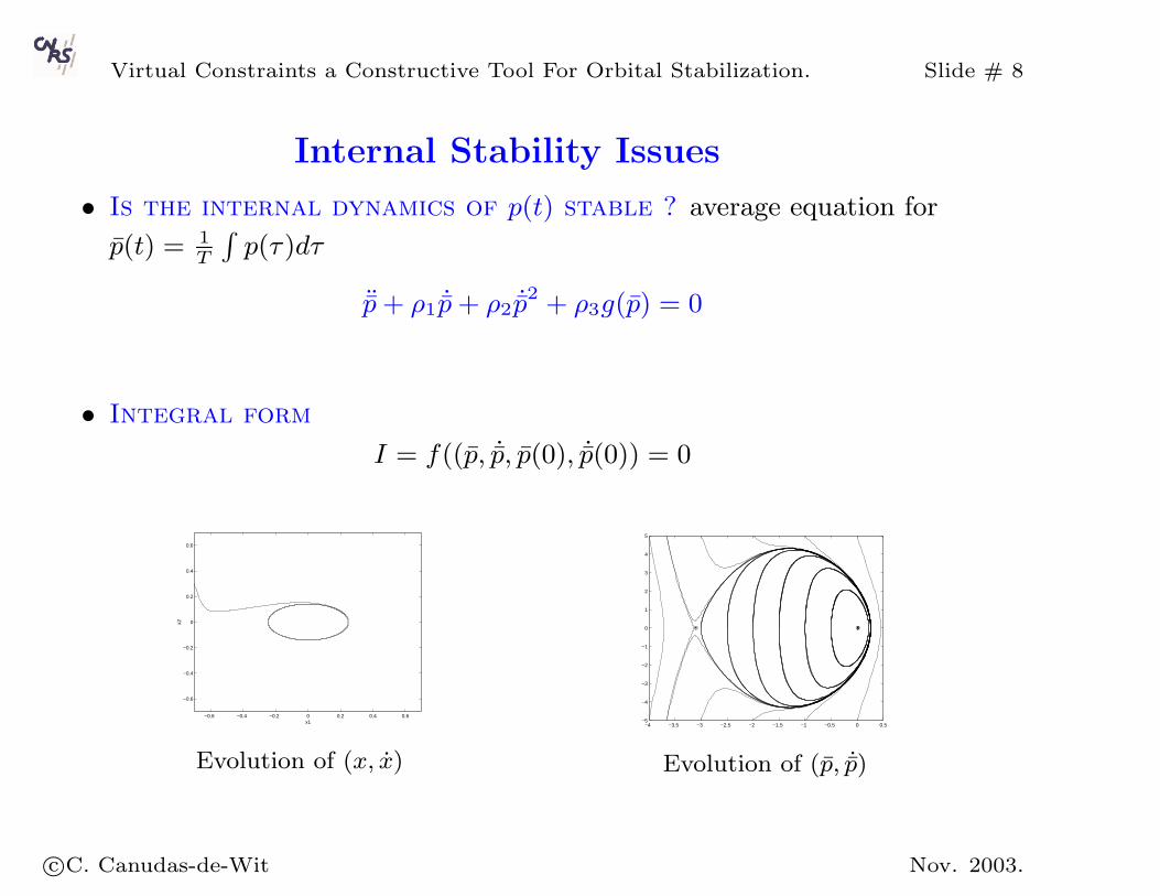
Internal Stability Issues
• Is the internal dynamics of p(t) stable ? average equation for
p(t) = 1T
∫p(τ)dτ
¨p+ ρ1 ˙p+ ρ2 ˙p2 + ρ3g(p) = 0
• Integral form
I = f((p, ˙p, p(0), ˙p(0)) = 0
−0.6 −0.4 −0.2 0 0.2 0.4 0.6
−0.6
−0.4
−0.2
0
0.2
0.4
0.6
x1
x2
Evolution of (x, x)
−4 −3.5 −3 −2.5 −2 −1.5 −1 −0.5 0 0.5−5
−4
−3
−2
−1
0
1
2
3
4
5
Evolution of (p, ˙p)
c©C. Canudas-de-Wit Nov. 2003.
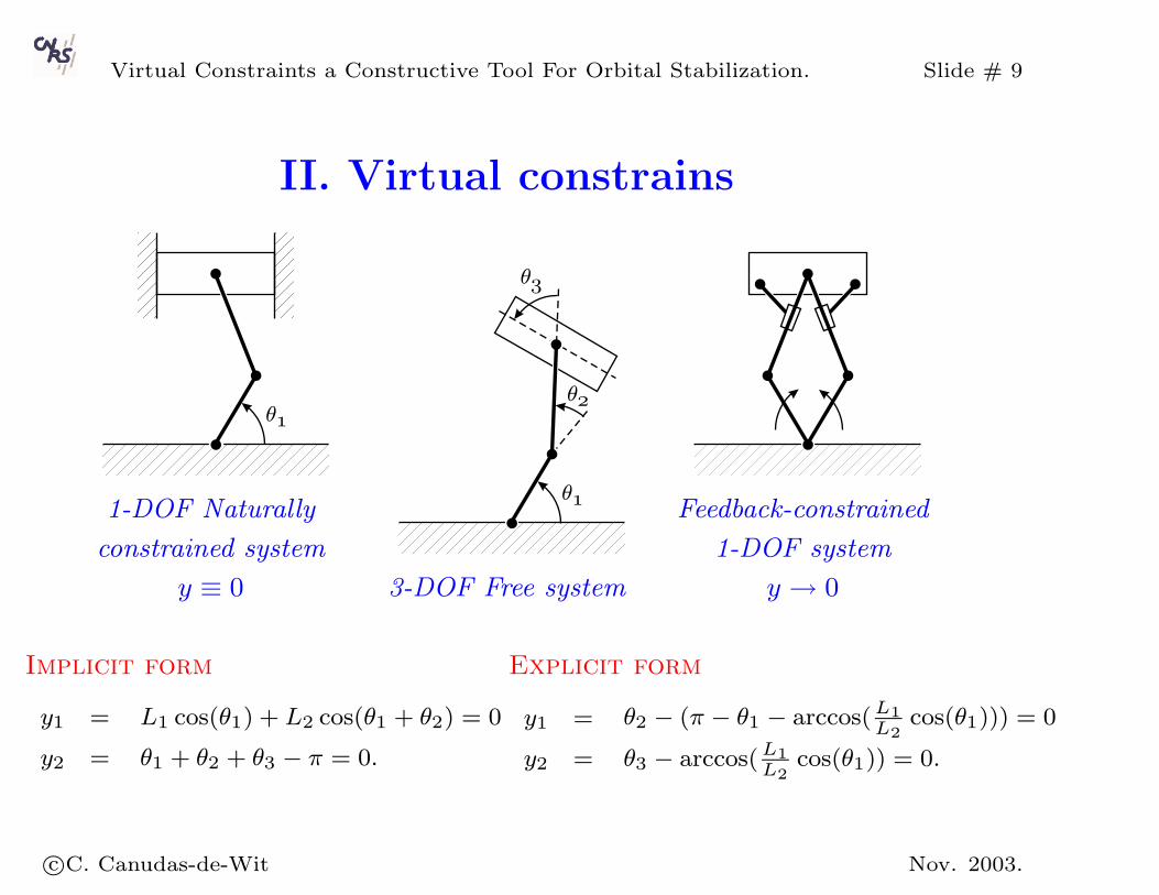
Virtual Constraints a Constructive Tool For Orbital Stabilization. Slide # 9
II. Virtual constrains
1-DOF Naturally
constrained system
y ≡ 0 3-DOF Free system
Feedback-constrained
1-DOF system
y → 0
Implicit form
y1 =
y2 =
L1 cos(θ1) + L2 cos(θ1 + θ2) = 0
θ1 + θ2 + θ3 − π = 0.
Explicit form
y1 =
y2 =
θ2 − (π − θ1 − arccos(L1L2
cos(θ1))) = 0
θ3 − arccos(L1L2
cos(θ1)) = 0.
c©C. Canudas-de-Wit Nov. 2003.
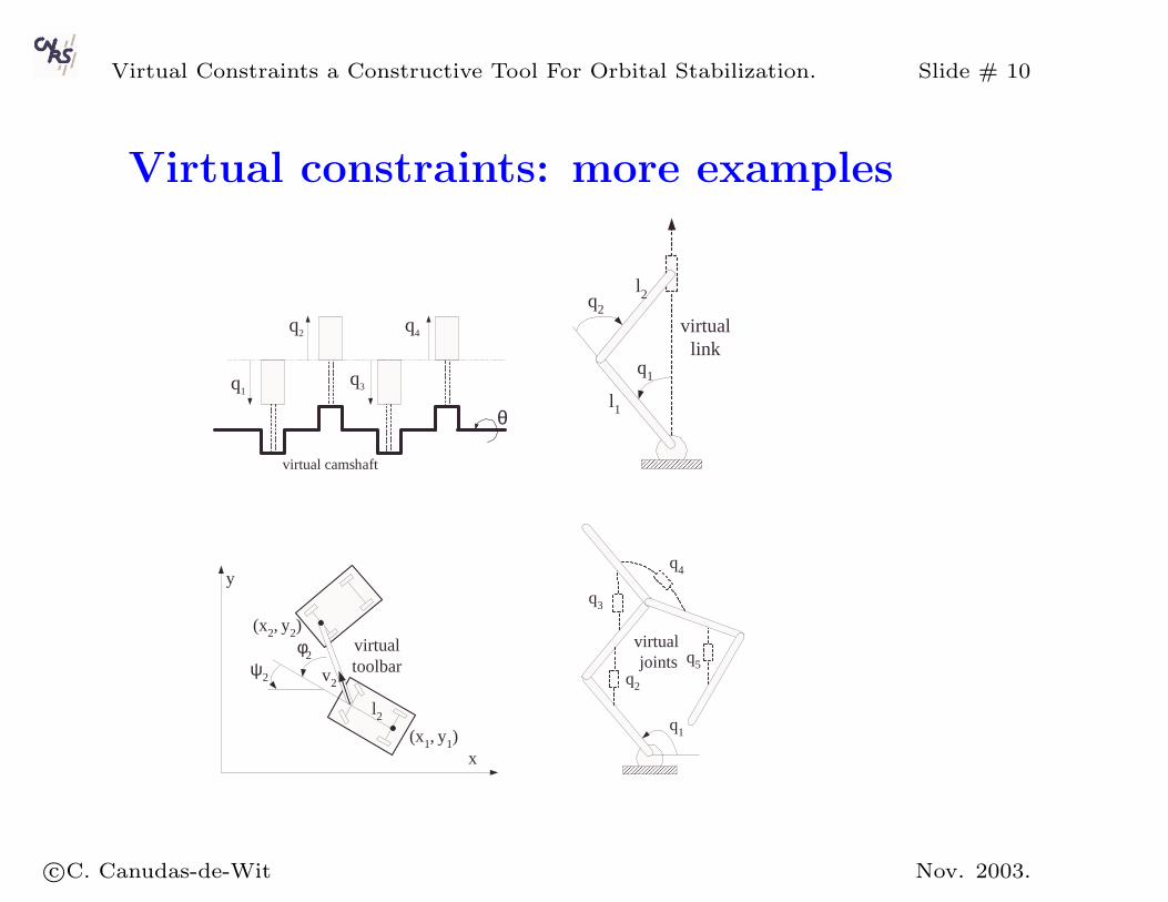
Virtual Constraints a Constructive Tool For Orbital Stabilization. Slide # 10
Virtual constraints: more examples
q4q2
q3q1
virtual camshaft
θl1
l2
q1
q2virtual
link
(x1, y1)
virtualtoolbar
(x2, y2)
ψ2
φ2
l2
x
y
v2
q1
q3
virtual joints
q4
q5q2
c©C. Canudas-de-Wit Nov. 2003.
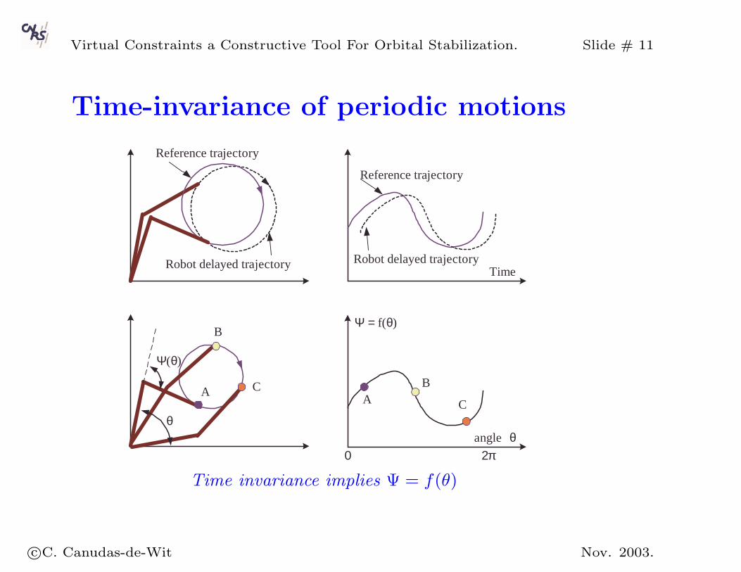
Virtual Constraints a Constructive Tool For Orbital Stabilization. Slide # 11
Time-invariance of periodic motions
Reference trajectory
Robot delayed trajectory
Reference trajectory
angle
TimeRobot delayed trajectory
Ψ = f(θ)
0 2π
Ψ(θ)
θθ
A A
B
C B
C
Time invariance implies Ψ = f(θ)
c©C. Canudas-de-Wit Nov. 2003.
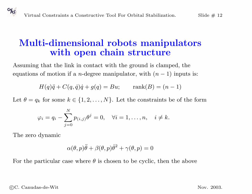
Virtual Constraints a Constructive Tool For Orbital Stabilization. Slide # 12
Multi-dimensional robots manipulatorswith open chain structure
Assuming that the link in contact with the ground is clamped, the
equations of motion if a n-degree manipulator, with (n− 1) inputs is:
H(q)q + C(q, q)q + g(q) = Bu; rank(B) = (n− 1)
Let θ = qk for some k ∈ 1, 2, . . . , N. Let the constraints be of the form
ϕi = qi −N∑j=0
p(i,j)θj = 0, ∀i = 1, . . . , n, i = k.
The zero dynamic
α(θ, p)θ + β(θ, p)θ2 + γ(θ, p) = 0
For the particular case where θ is chosen to be cyclic, then the above
c©C. Canudas-de-Wit Nov. 2003.
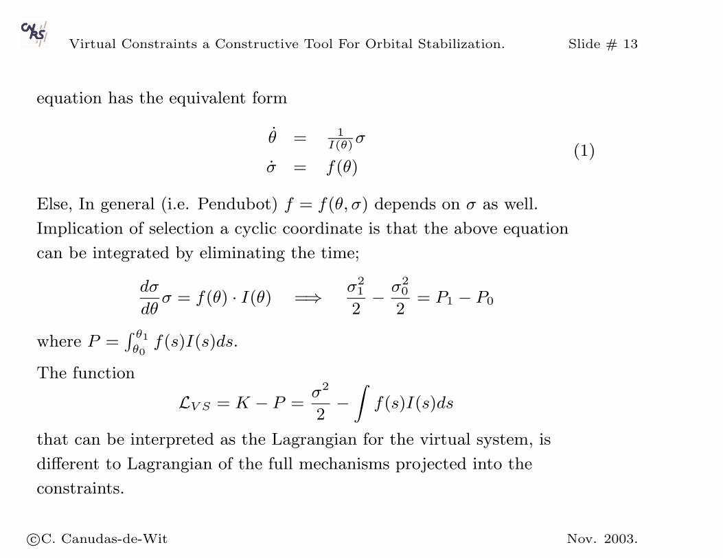
Virtual Constraints a Constructive Tool For Orbital Stabilization. Slide # 13
equation has the equivalent form
θ =
σ =
1I(θ)
σ
f(θ)(1)
Else, In general (i.e. Pendubot) f = f(θ, σ) depends on σ as well.
Implication of selection a cyclic coordinate is that the above equation
can be integrated by eliminating the time;
dσ
dθσ = f(θ) · I(θ) =⇒ σ2
1
2− σ2
0
2= P1 − P0
where P =∫ θ1θ0f(s)I(s)ds.
The function
LV S = K − P =σ2
2−
∫f(s)I(s)ds
that can be interpreted as the Lagrangian for the virtual system, is
different to Lagrangian of the full mechanisms projected into the
constraints.
c©C. Canudas-de-Wit Nov. 2003.
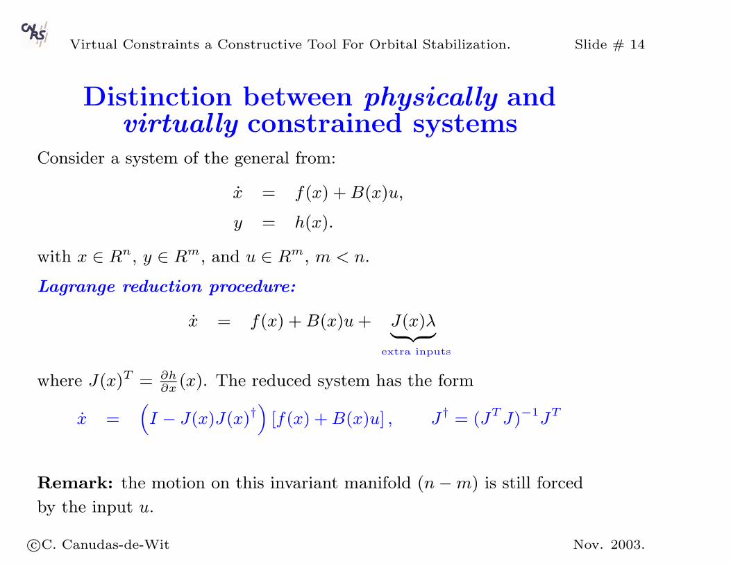
Virtual Constraints a Constructive Tool For Orbital Stabilization. Slide # 14
Distinction between physically andvirtually constrained systems
Consider a system of the general from:
x = f(x) +B(x)u,
y = h(x).
with x ∈ Rn, y ∈ Rm, and u ∈ Rm, m < n.
Lagrange reduction procedure:
x = f(x) +B(x)u+ J(x)λ︸ ︷︷ ︸extra inputs
where J(x)T = ∂h∂x
(x). The reduced system has the form
x =(I − J(x)J(x)†
)[f(x) +B(x)u] , J† = (JTJ)−1JT
Remark: the motion on this invariant manifold (n−m) is still forced
by the input u.
c©C. Canudas-de-Wit Nov. 2003.
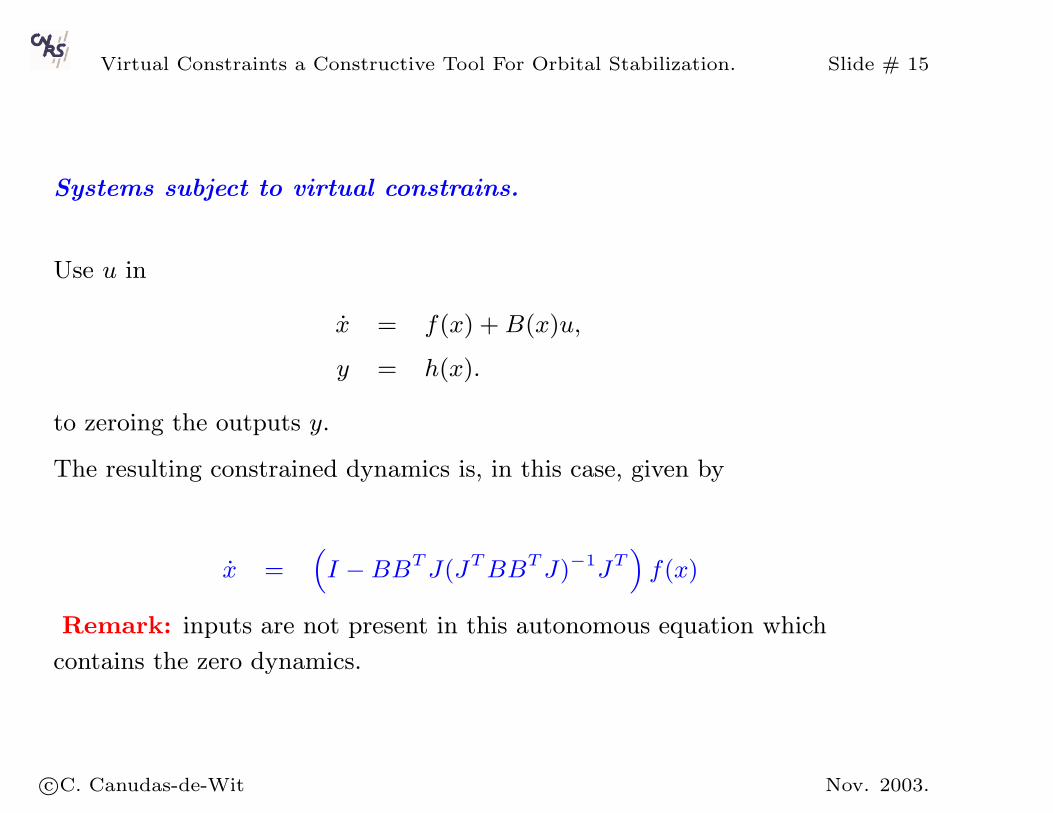
Virtual Constraints a Constructive Tool For Orbital Stabilization. Slide # 15
Systems subject to virtual constrains.
Use u in
x = f(x) +B(x)u,
y = h(x).
to zeroing the outputs y.
The resulting constrained dynamics is, in this case, given by
x =(I −BBTJ(JTBBTJ)−1JT
)f(x)
Remark: inputs are not present in this autonomous equation which
contains the zero dynamics.
c©C. Canudas-de-Wit Nov. 2003.
Virtual Constraints a Constructive Tool For Orbital Stabilization. Slide # 16
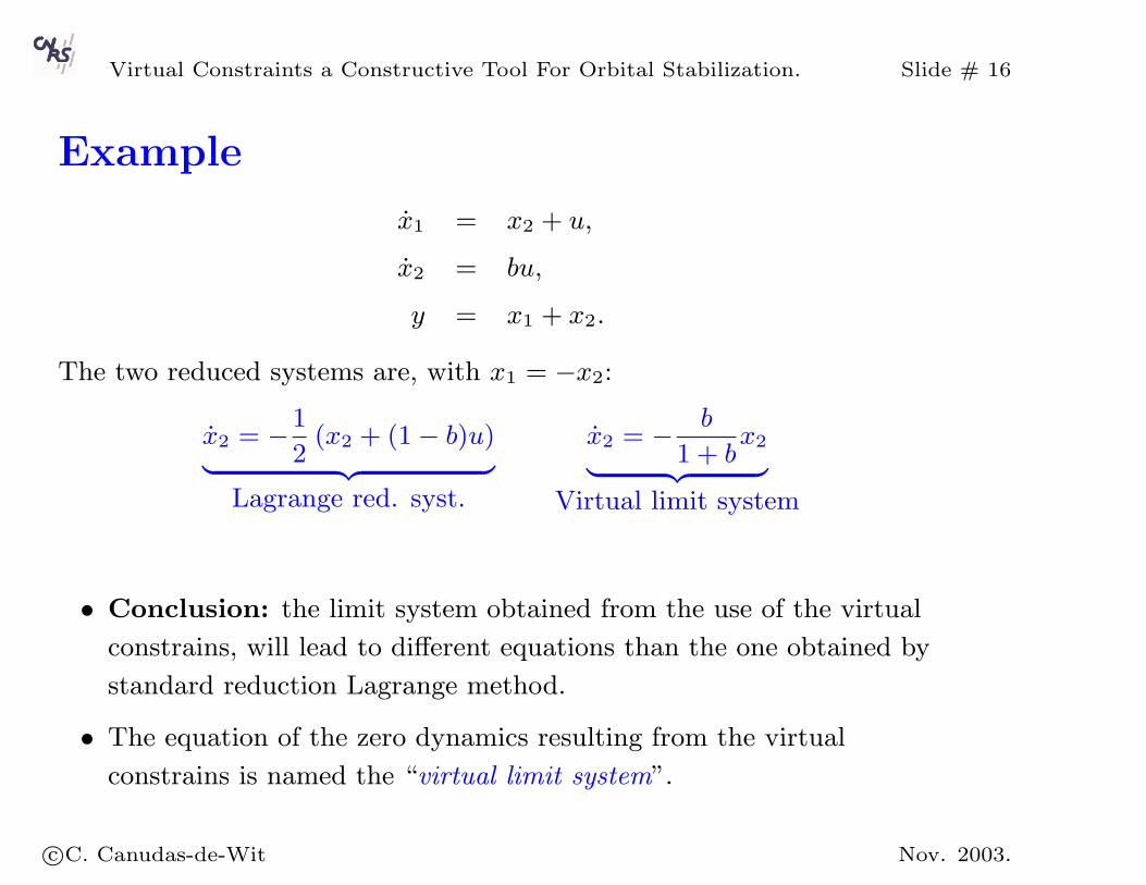
Example
x1 = x2 + u,
x2 = bu,
y = x1 + x2.
The two reduced systems are, with x1 = −x2:
x2 = −1
2(x2 + (1 − b)u)︸ ︷︷ ︸
Lagrange red. syst.
x2 = − b
1 + bx2︸ ︷︷ ︸
Virtual limit system
• Conclusion: the limit system obtained from the use of the virtual
constrains, will lead to different equations than the one obtained by
standard reduction Lagrange method.
• The equation of the zero dynamics resulting from the virtual
constrains is named the “virtual limit system”.
c©C. Canudas-de-Wit Nov. 2003.
Virtual Constraints a Constructive Tool For Orbital Stabilization. Slide # 17
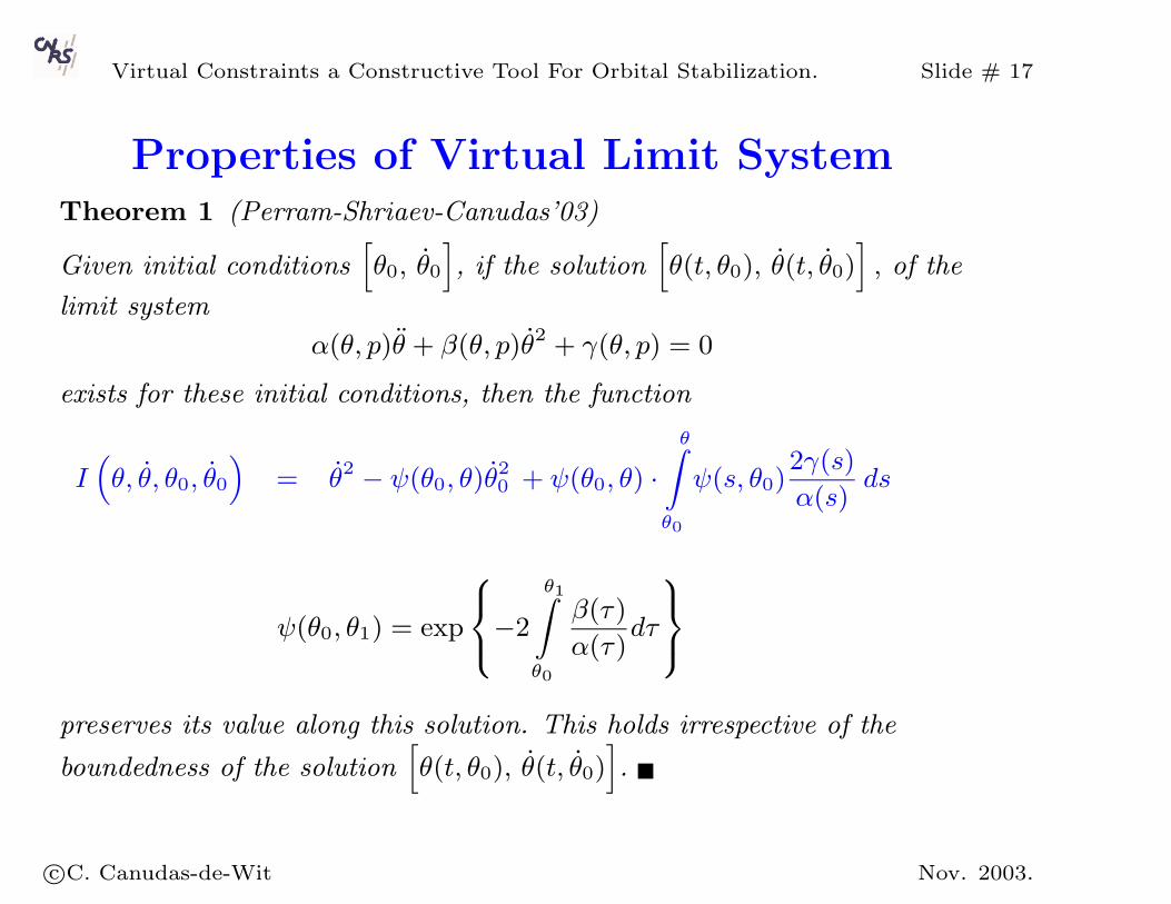
Properties of Virtual Limit SystemTheorem 1 (Perram-Shriaev-Canudas’03)
Given initial conditions[θ0, θ0
], if the solution
[θ(t, θ0), θ(t, θ0)
], of the
limit system
α(θ, p)θ + β(θ, p)θ2 + γ(θ, p) = 0
exists for these initial conditions, then the function
I(θ, θ, θ0, θ0
)= θ2 − ψ(θ0, θ)θ
20 + ψ(θ0, θ) ·
θ∫θ0
ψ(s, θ0)2γ(s)
α(s)ds
ψ(θ0, θ1) = exp
−2
θ1∫θ0
β(τ)
α(τ)dτ
preserves its value along this solution. This holds irrespective of the
boundedness of the solution[θ(t, θ0), θ(t, θ0)
].
c©C. Canudas-de-Wit Nov. 2003.
Virtual Constraints a Constructive Tool For Orbital Stabilization. Slide # 18
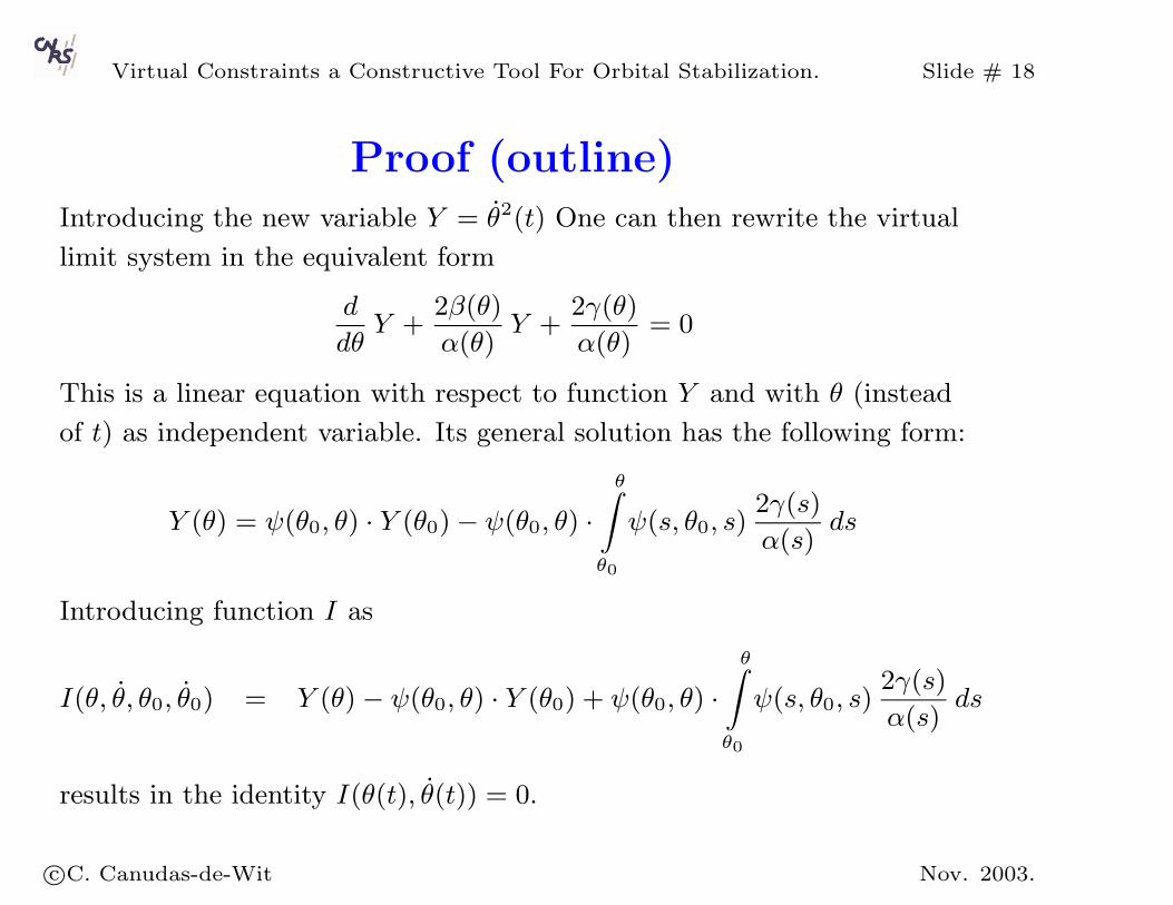
Proof (outline)Introducing the new variable Y = θ2(t) One can then rewrite the virtual
limit system in the equivalent form
d
dθY +
2β(θ)
α(θ)Y +
2γ(θ)
α(θ)= 0
This is a linear equation with respect to function Y and with θ (instead
of t) as independent variable. Its general solution has the following form:
Y (θ) = ψ(θ0, θ) · Y (θ0) − ψ(θ0, θ) ·θ∫
θ0
ψ(s, θ0, s)2γ(s)
α(s)ds
Introducing function I as
I(θ, θ, θ0, θ0) = Y (θ) − ψ(θ0, θ) · Y (θ0) + ψ(θ0, θ) ·θ∫
θ0
ψ(s, θ0, s)2γ(s)
α(s)ds
results in the identity I(θ(t), θ(t)) = 0.
c©C. Canudas-de-Wit Nov. 2003.
Virtual Constraints a Constructive Tool For Orbital Stabilization. Slide # 19
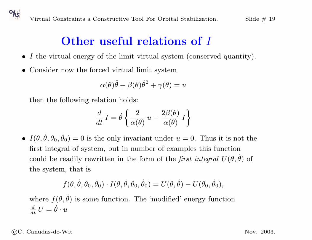
Other useful relations of I• I the virtual energy of the limit virtual system (conserved quantity).
• Consider now the forced virtual limit system
α(θ)θ + β(θ)θ2 + γ(θ) = u
then the following relation holds:
d
dtI = θ
2
α(θ)u− 2β(θ)
α(θ)I
• I(θ, θ, θ0, θ0) = 0 is the only invariant under u = 0. Thus it is not the
first integral of system, but in number of examples this function
could be readily rewritten in the form of the first integral U(θ, θ) of
the system, that is
f(θ, θ, θ0, θ0) · I(θ, θ, θ0, θ0) = U(θ, θ) − U(θ0, θ0),
where f(θ, θ) is some function. The ‘modified’ energy functionddtU = θ · u
c©C. Canudas-de-Wit Nov. 2003.
Virtual Constraints a Constructive Tool For Orbital Stabilization. Slide # 20
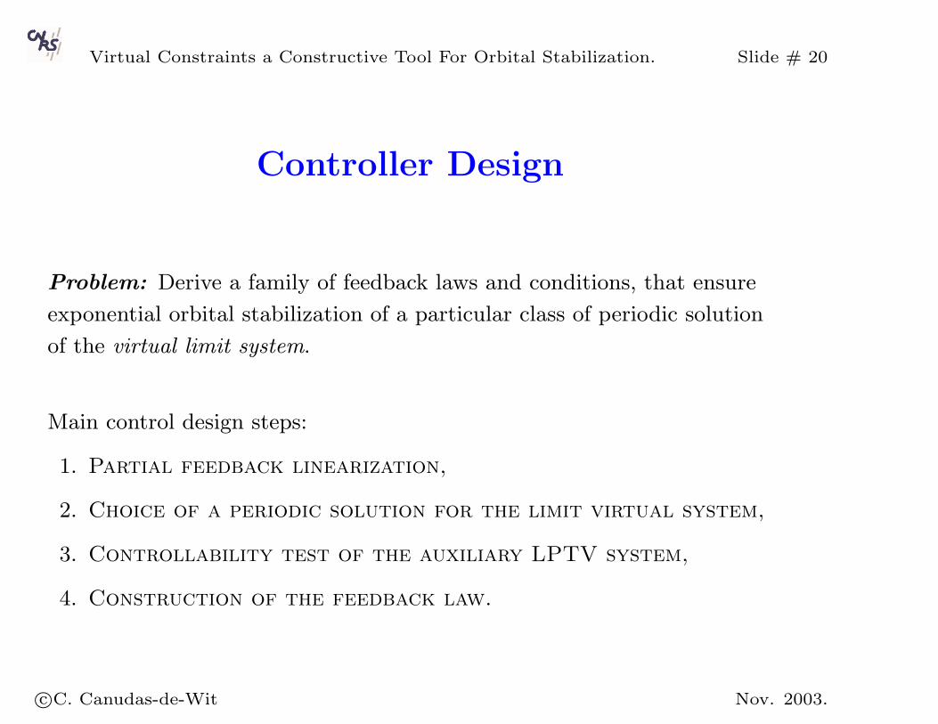
Controller Design
Problem: Derive a family of feedback laws and conditions, that ensure
exponential orbital stabilization of a particular class of periodic solution
of the virtual limit system.
Main control design steps:
1. Partial feedback linearization,
2. Choice of a periodic solution for the limit virtual system,
3. Controllability test of the auxiliary LPTV system,
4. Construction of the feedback law.
c©C. Canudas-de-Wit Nov. 2003.
Virtual Constraints a Constructive Tool For Orbital Stabilization. Slide # 21
1. Partial Feedback LinearizationThe original nonlinear system is first transformed, via partial feedback
linearization, to a form
α(θ)θ + β(θ)θ2 + γ(θ)︸ ︷︷ ︸virtual limit system
= g1(θ, θ, y, y) + g2(θ, θ, y, y) · v
y = v
Here y ∈ Rn−1, θ ∈ R1; v ∈ Rn−1. The gi, are smooth functions
g1(θ, θ, 0, 0) + g2(θ, θ, 0, 0) · v = 0, v = 0(n−1)×1.
In turn, due to the smoothness of g1 = gy(θ, θ, y, y) · y + gy(θ, θ, y, y) · y.This yields the Auxiliary System:
I = θ
2
α(θ)[gy · y + gy · y + g2 · v] − 2β(θ)
α(θ)I
y = v
c©C. Canudas-de-Wit Nov. 2003.
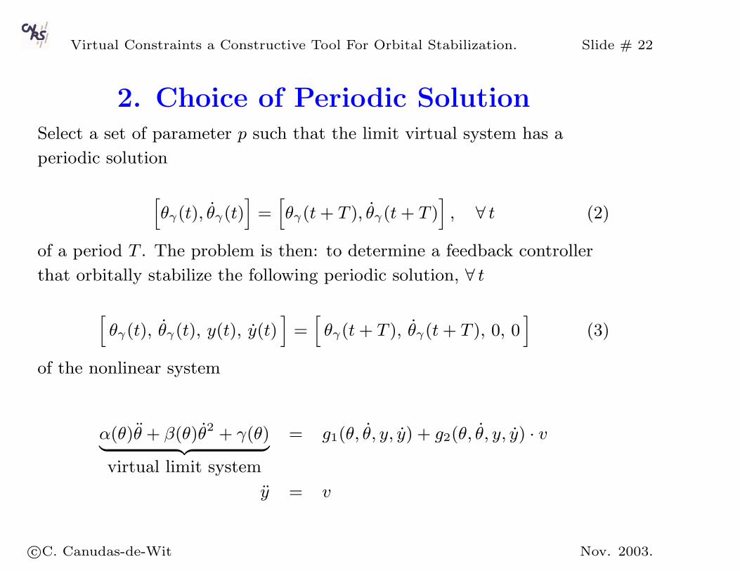
Virtual Constraints a Constructive Tool For Orbital Stabilization. Slide # 22
2. Choice of Periodic SolutionSelect a set of parameter p such that the limit virtual system has a
periodic solution
[θγ(t), θγ(t)
]=
[θγ(t+ T ), θγ(t+ T )
], ∀ t (2)
of a period T . The problem is then: to determine a feedback controller
that orbitally stabilize the following periodic solution, ∀ t[θγ(t), θγ(t), y(t), y(t)
]=
[θγ(t+ T ), θγ(t+ T ), 0, 0
](3)
of the nonlinear system
α(θ)θ + β(θ)θ2 + γ(θ)︸ ︷︷ ︸virtual limit system
= g1(θ, θ, y, y) + g2(θ, θ, y, y) · v
y = v
c©C. Canudas-de-Wit Nov. 2003.
Virtual Constraints a Constructive Tool For Orbital Stabilization. Slide # 23
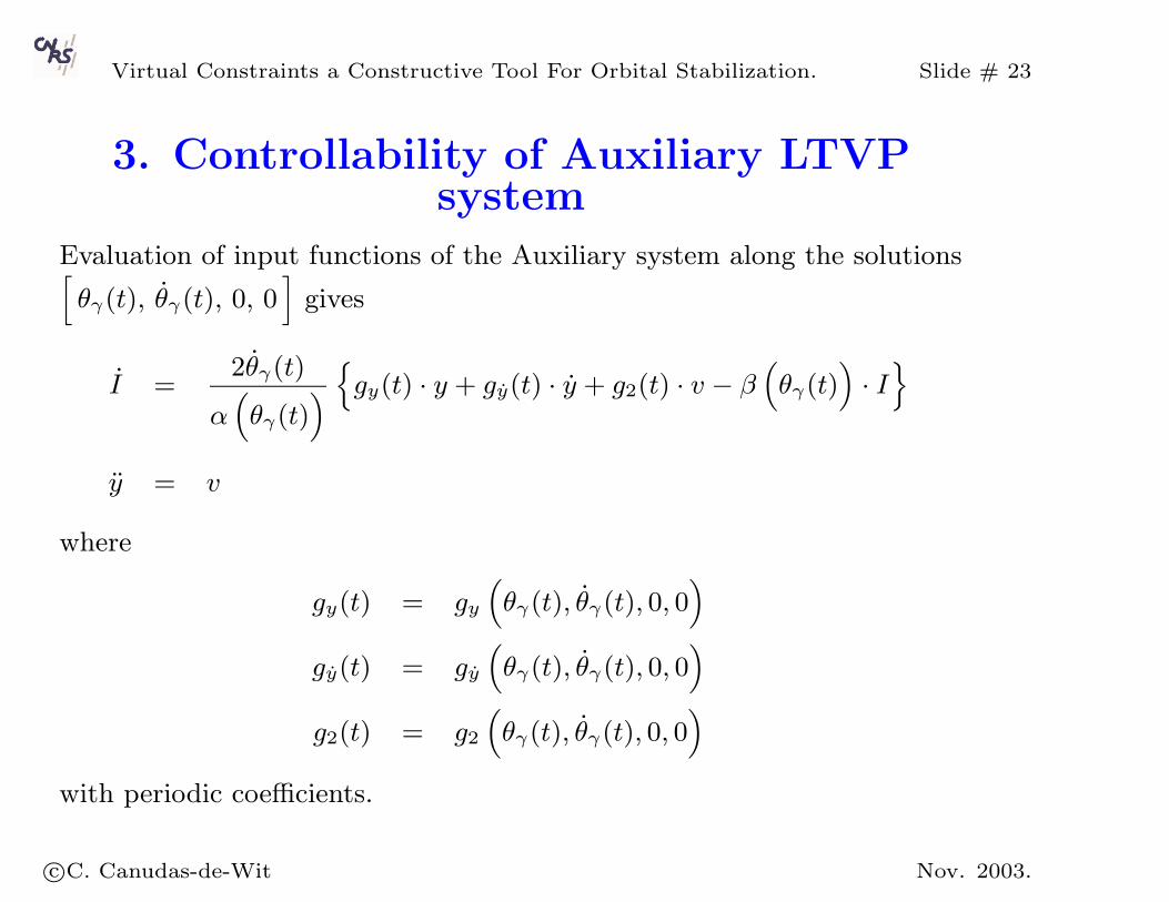
3. Controllability of Auxiliary LTVPsystem
Evaluation of input functions of the Auxiliary system along the solutions[θγ(t), θγ(t), 0, 0
]gives
I =2θγ(t)
α(θγ(t)
) gy(t) · y + gy(t) · y + g2(t) · v − β
(θγ(t)
)· I
y = v
where
gy(t) = gy(θγ(t), θγ(t), 0, 0
)
gy(t) = gy(θγ(t), θγ(t), 0, 0
)
g2(t) = g2(θγ(t), θγ(t), 0, 0
)with periodic coefficients.
c©C. Canudas-de-Wit Nov. 2003.
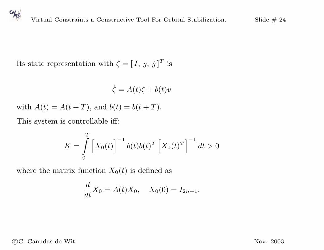
Virtual Constraints a Constructive Tool For Orbital Stabilization. Slide # 24
Its state representation with ζ = [ I, y, y ]T is
ζ = A(t)ζ + b(t)v
with A(t) = A(t+ T ), and b(t) = b(t+ T ).
This system is controllable iff:
K =
T∫0
[X0(t)
]−1
b(t)b(t)T[X0(t)T
]−1
dt > 0
where the matrix function X0(t) is defined as
d
dtX0 = A(t)X0, X0(0) = I2n+1.
c©C. Canudas-de-Wit Nov. 2003.
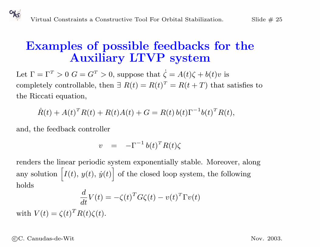
Virtual Constraints a Constructive Tool For Orbital Stabilization. Slide # 25
Examples of possible feedbacks for theAuxiliary LTVP system
Let Γ = ΓT > 0 G = GT > 0, suppose that ζ = A(t)ζ + b(t)v is
completely controllable, then ∃ R(t) = R(t)T = R(t+ T ) that satisfies to
the Riccati equation,
R(t) +A(t)TR(t) +R(t)A(t) +G = R(t) b(t)Γ−1b(t)TR(t),
and, the feedback controller
v = −Γ−1 b(t)TR(t)ζ
renders the linear periodic system exponentially stable. Moreover, along
any solution[I(t), y(t), y(t)
]of the closed loop system, the following
holdsd
dtV (t) = −ζ(t)TGζ(t) − v(t)T Γv(t)
with V (t) = ζ(t)TR(t)ζ(t).
c©C. Canudas-de-Wit Nov. 2003.
Virtual Constraints a Constructive Tool For Orbital Stabilization. Slide # 26
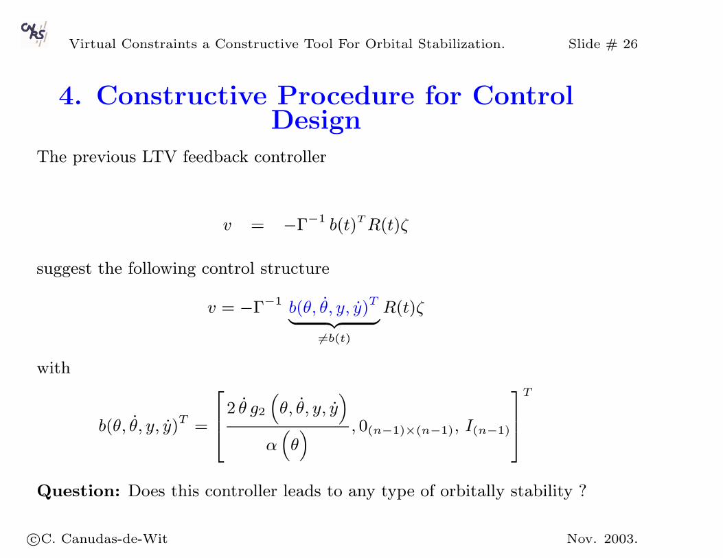
4. Constructive Procedure for ControlDesign
The previous LTV feedback controller
v = −Γ−1 b(t)TR(t)ζ
suggest the following control structure
v = −Γ−1 b(θ, θ, y, y)T︸ ︷︷ ︸=b(t)
R(t)ζ
with
b(θ, θ, y, y)T =
2 θ g2
(θ, θ, y, y
)α(θ) , 0(n−1)×(n−1), I(n−1)
T
Question: Does this controller leads to any type of orbitally stability ?
c©C. Canudas-de-Wit Nov. 2003.
Virtual Constraints a Constructive Tool For Orbital Stabilization. Slide # 27
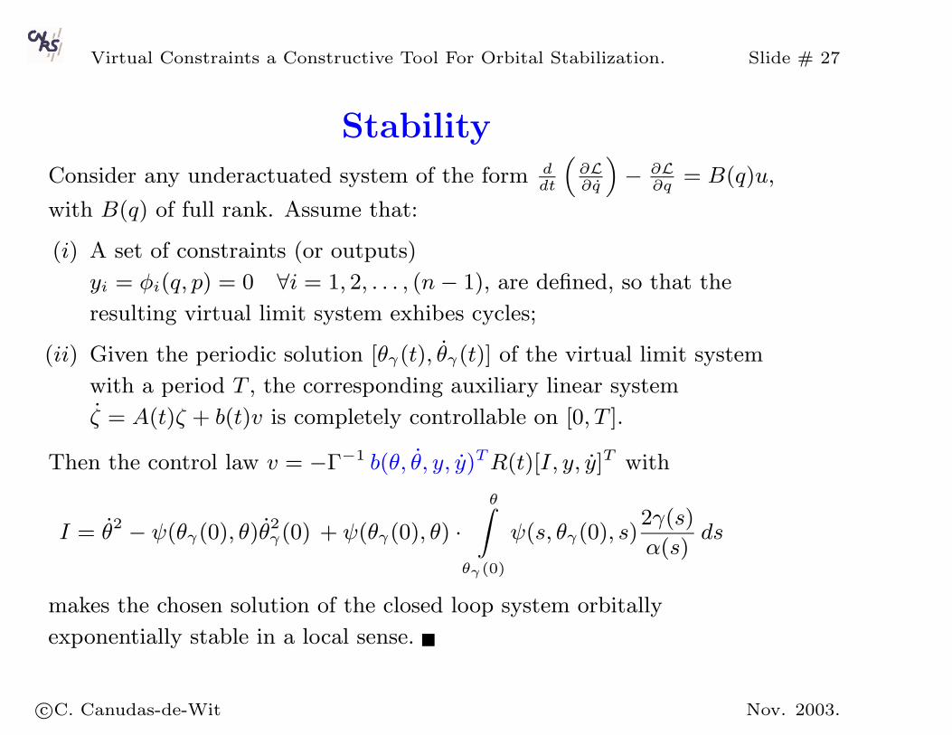
Stability
Consider any underactuated system of the form ddt
(∂L∂q
)− ∂L
∂q= B(q)u,
with B(q) of full rank. Assume that:
(i) A set of constraints (or outputs)
yi = φi(q, p) = 0 ∀i = 1, 2, . . . , (n− 1), are defined, so that the
resulting virtual limit system exhibes cycles;
(ii) Given the periodic solution [θγ(t), θγ(t)] of the virtual limit system
with a period T , the corresponding auxiliary linear system
ζ = A(t)ζ + b(t)v is completely controllable on [0, T ].
Then the control law v = −Γ−1 b(θ, θ, y, y)TR(t)[I, y, y]T with
I = θ2 − ψ(θγ(0), θ)θ2γ(0) + ψ(θγ(0), θ) ·θ∫
θγ(0)
ψ(s, θγ(0), s)2γ(s)
α(s)ds
makes the chosen solution of the closed loop system orbitally
exponentially stable in a local sense.
c©C. Canudas-de-Wit Nov. 2003.
Virtual Constraints a Constructive Tool For Orbital Stabilization. Slide # 28
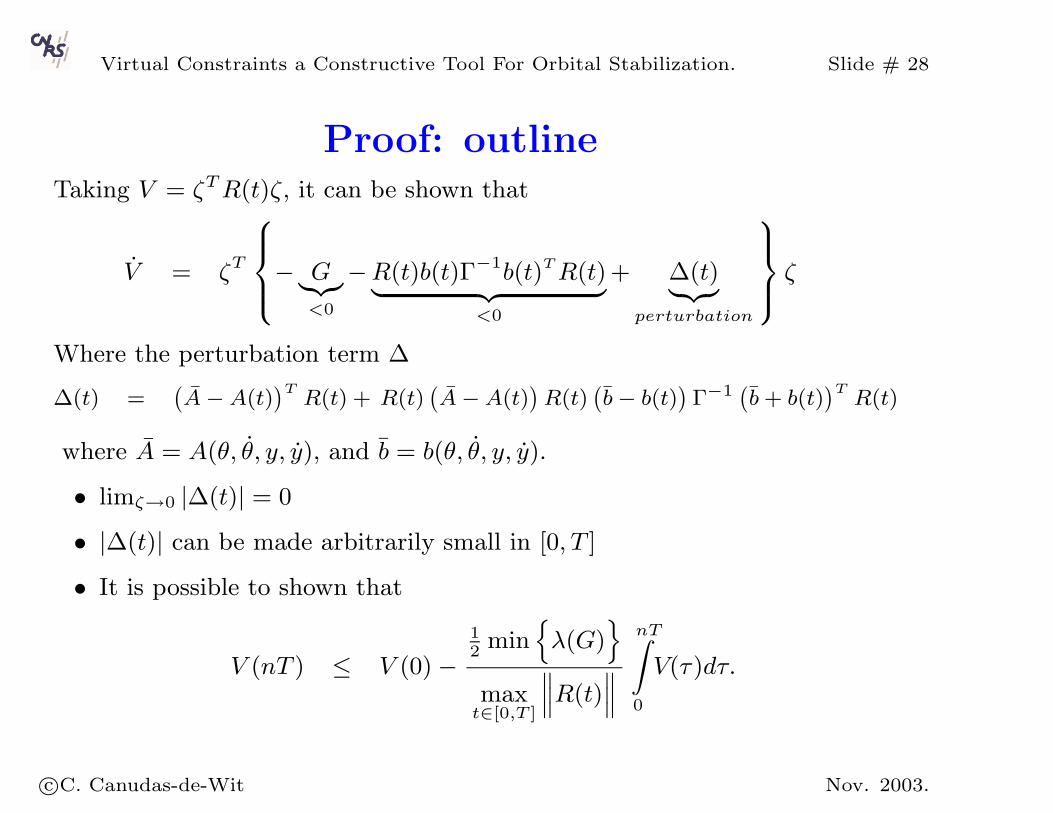
Proof: outlineTaking V = ζTR(t)ζ, it can be shown that
V = ζT
− G︸︷︷︸
<0
−R(t)b(t)Γ−1b(t)TR(t)︸ ︷︷ ︸<0
+ ∆(t)︸︷︷︸perturbation
ζ
Where the perturbation term ∆
∆(t) =(A − A(t)
)TR(t) + R(t)
(A − A(t)
)R(t)
(b − b(t)
)Γ−1
(b + b(t)
)TR(t)
where A = A(θ, θ, y, y), and b = b(θ, θ, y, y).
• limζ→0 |∆(t)| = 0
• |∆(t)| can be made arbitrarily small in [0, T ]
• It is possible to shown that
V (nT ) ≤ V (0) −12
minλ(G)
maxt∈[0,T ]
∥∥∥R(t)∥∥∥
nT∫0
V(τ)dτ.
c©C. Canudas-de-Wit Nov. 2003.
Virtual Constraints a Constructive Tool For Orbital Stabilization. Slide # 29
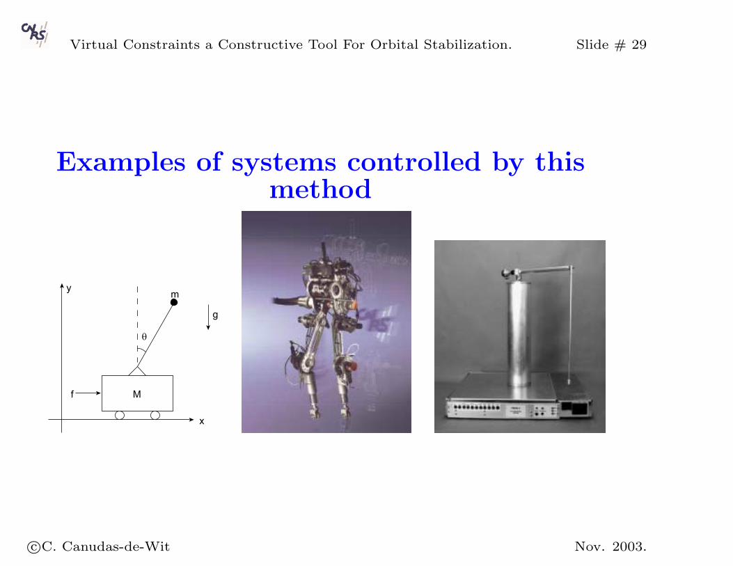
Examples of systems controlled by thismethod
c©C. Canudas-de-Wit Nov. 2003.
Virtual Constraints a Constructive Tool For Orbital Stabilization. Slide # 30
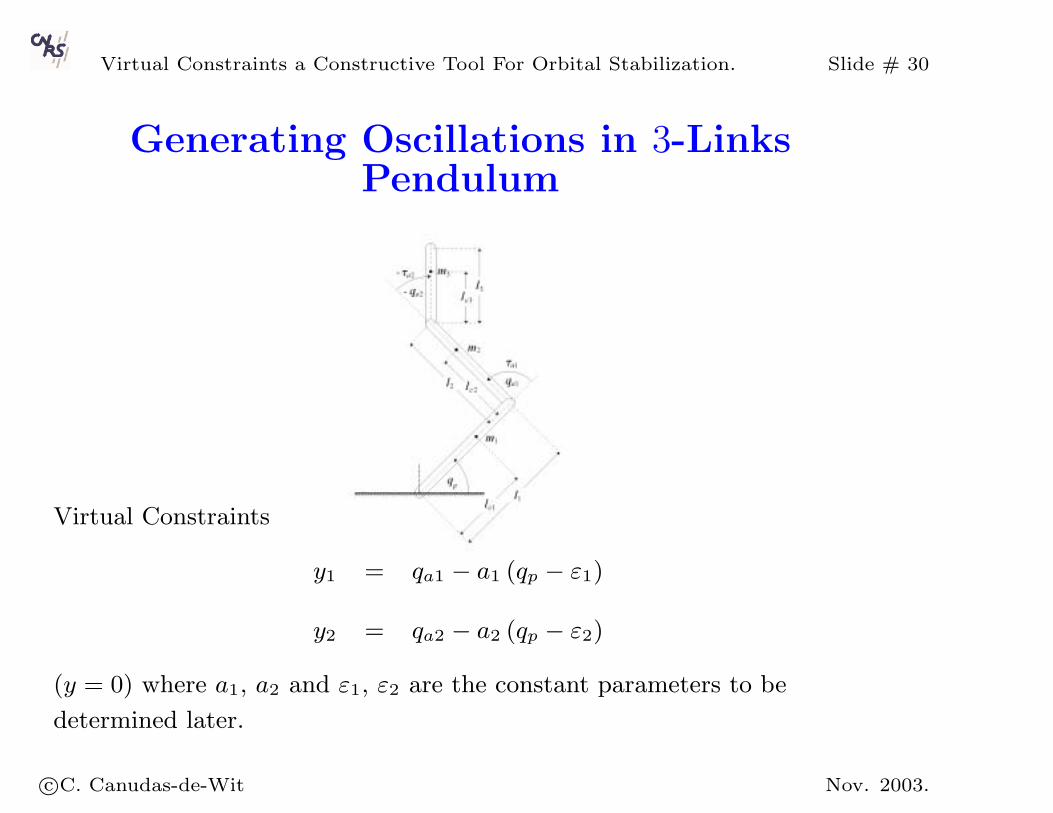
Generating Oscillations in 3-LinksPendulum
Virtual Constraints
y1 = qa1 − a1 (qp − ε1)
y2 = qa2 − a2 (qp − ε2)
(y = 0) where a1, a2 and ε1, ε2 are the constant parameters to be
determined later.
c©C. Canudas-de-Wit Nov. 2003.
Virtual Constraints a Constructive Tool For Orbital Stabilization. Slide # 31
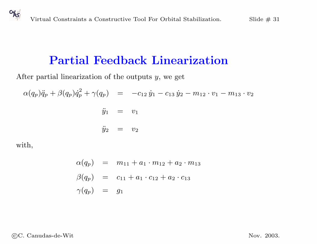
Partial Feedback LinearizationAfter partial linearization of the outputs y, we get
α(qp)qp + β(qp)q2p + γ(qp) = −c12 y1 − c13 y2 −m12 · v1 −m13 · v2
y1 = v1
y2 = v2
with,
α(qp) = m11 + a1 ·m12 + a2 ·m13
β(qp) = c11 + a1 · c12 + a2 · c13γ(qp) = g1
c©C. Canudas-de-Wit Nov. 2003.
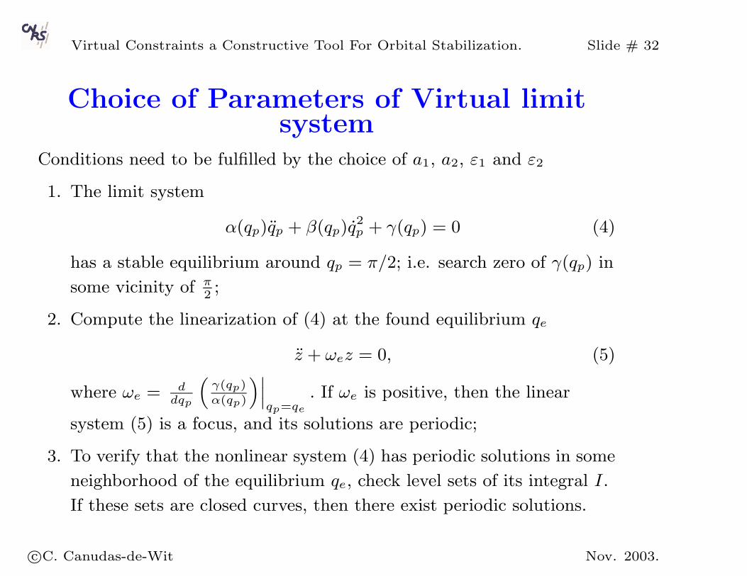
Virtual Constraints a Constructive Tool For Orbital Stabilization. Slide # 32
Choice of Parameters of Virtual limitsystem
Conditions need to be fulfilled by the choice of a1, a2, ε1 and ε2
1. The limit system
α(qp)qp + β(qp)q2p + γ(qp) = 0 (4)
has a stable equilibrium around qp = π/2; i.e. search zero of γ(qp) in
some vicinity of π2
;
2. Compute the linearization of (4) at the found equilibrium qe
z + ωez = 0, (5)
where ωe = ddqp
(γ(qp)
α(qp)
)∣∣∣qp=qe
. If ωe is positive, then the linear
system (5) is a focus, and its solutions are periodic;
3. To verify that the nonlinear system (4) has periodic solutions in some
neighborhood of the equilibrium qe, check level sets of its integral I.
If these sets are closed curves, then there exist periodic solutions.
c©C. Canudas-de-Wit Nov. 2003.
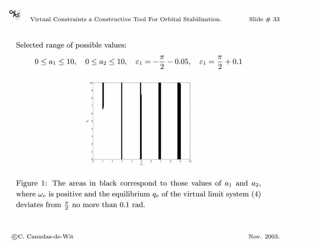
Virtual Constraints a Constructive Tool For Orbital Stabilization. Slide # 33
Selected range of possible values:
0 ≤ a1 ≤ 10, 0 ≤ a2 ≤ 10, ε1 = −π2− 0.05, ε1 =
π
2+ 0.1
0 1 2 3 4 5 6 7 8 9 100
1
2
3
4
5
6
7
8
9
10
a1
a 2
Figure 1: The areas in black correspond to those values of a1 and a2,
where ωe is positive and the equilibrium qe of the virtual limit system (4)
deviates from π2
no more than 0.1 rad.
c©C. Canudas-de-Wit Nov. 2003.
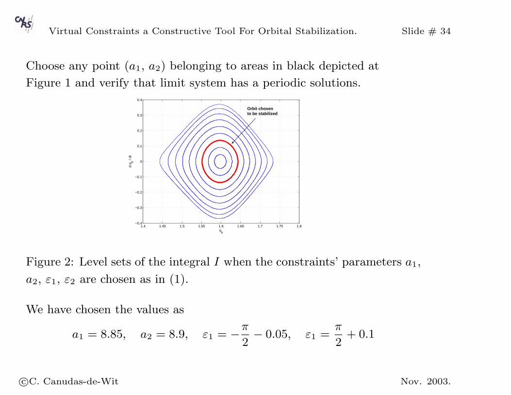
Virtual Constraints a Constructive Tool For Orbital Stabilization. Slide # 34
Choose any point (a1, a2) belonging to areas in black depicted at
Figure 1 and verify that limit system has a periodic solutions.
1.4 1.45 1.5 1.55 1.6 1.65 1.7 1.75 1.8−0.4
−0.3
−0.2
−0.1
0
0.1
0.2
0.3
0.4
qp
d q p /
dt
Orbit chosen to be stabilized
Figure 2: Level sets of the integral I when the constraints’ parameters a1,
a2, ε1, ε2 are chosen as in (1).
We have chosen the values as
a1 = 8.85, a2 = 8.9, ε1 = −π2− 0.05, ε1 =
π
2+ 0.1
c©C. Canudas-de-Wit Nov. 2003.
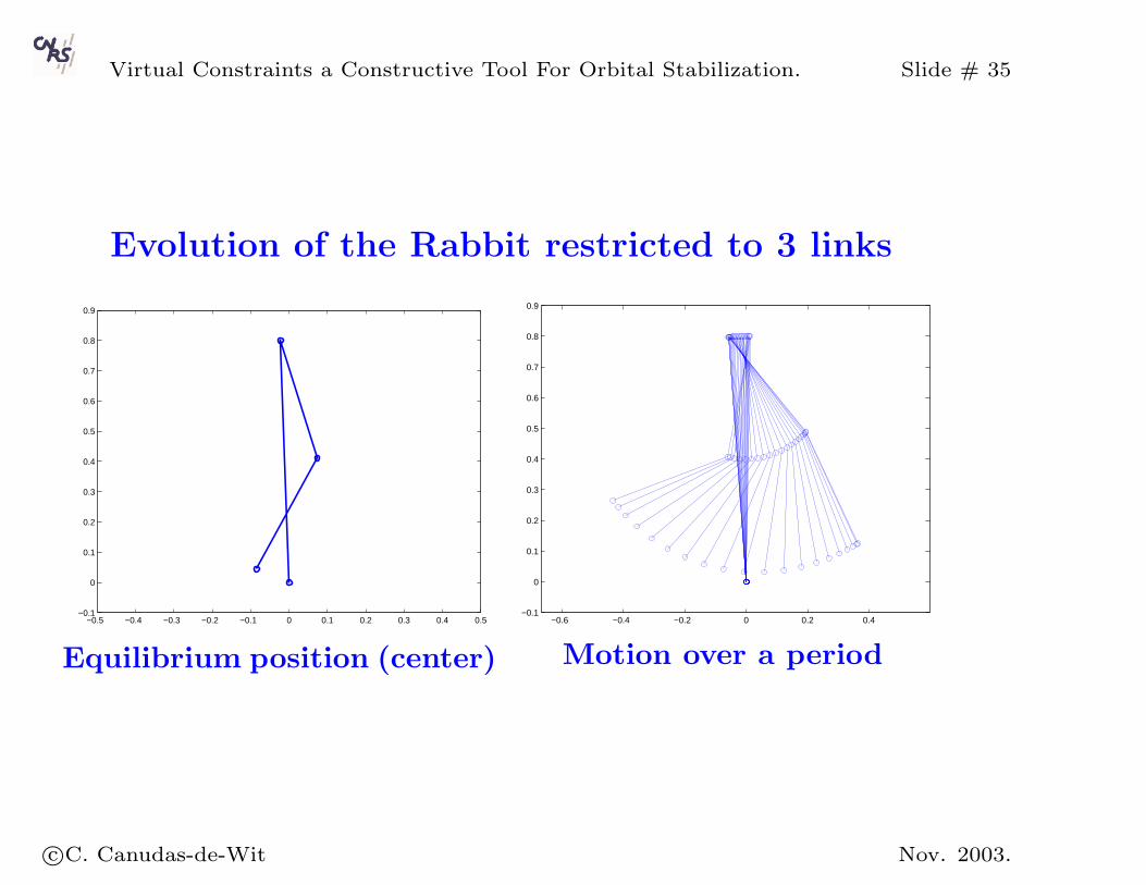
Virtual Constraints a Constructive Tool For Orbital Stabilization. Slide # 35
Evolution of the Rabbit restricted to 3 links
−0.5 −0.4 −0.3 −0.2 −0.1 0 0.1 0.2 0.3 0.4 0.5−0.1
0
0.1
0.2
0.3
0.4
0.5
0.6
0.7
0.8
0.9
Equilibrium position (center)−0.6 −0.4 −0.2 0 0.2 0.4
−0.1
0
0.1
0.2
0.3
0.4
0.5
0.6
0.7
0.8
0.9
Motion over a period
c©C. Canudas-de-Wit Nov. 2003.
Virtual Constraints a Constructive Tool For Orbital Stabilization. Slide # 36
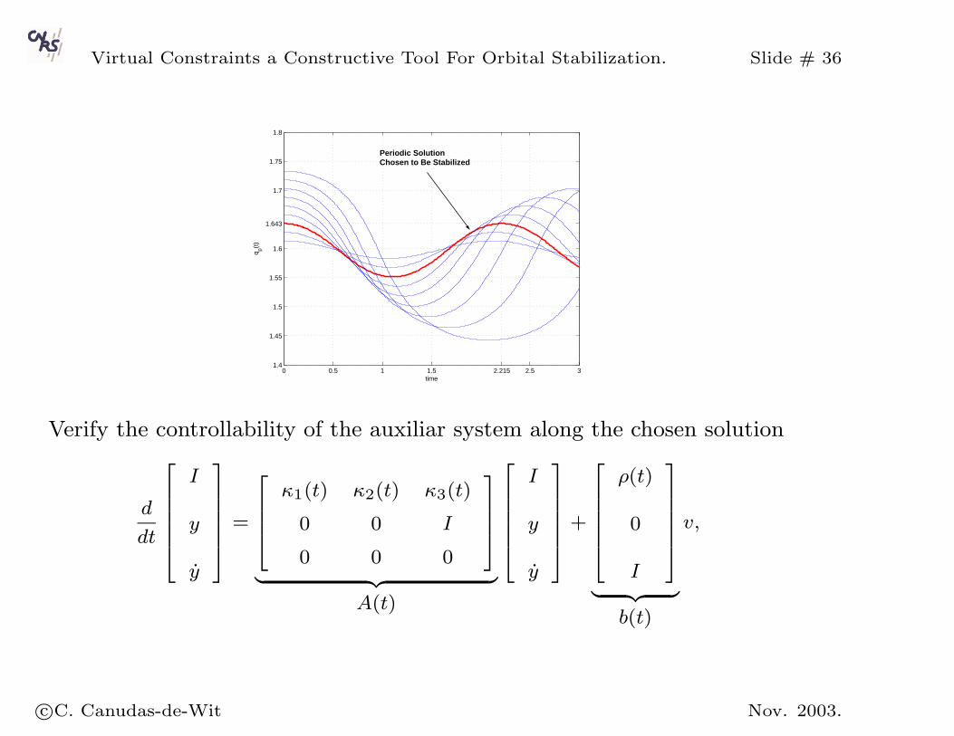
0 0.5 1 1.5 2.215 2.5 31.4
1.45
1.5
1.55
1.6
1.643
1.7
1.75
1.8
time
q p(t)
Periodic Solution Chosen to Be Stabilized
Verify the controllability of the auxiliar system along the chosen solution
d
dt
I
y
y
=
κ1(t) κ2(t) κ3(t)
0 0 I
0 0 0
︸ ︷︷ ︸A(t)
I
y
y
+
ρ(t)
0
I
︸ ︷︷ ︸b(t)
v,
c©C. Canudas-de-Wit Nov. 2003.
Virtual Constraints a Constructive Tool For Orbital Stabilization. Slide # 37
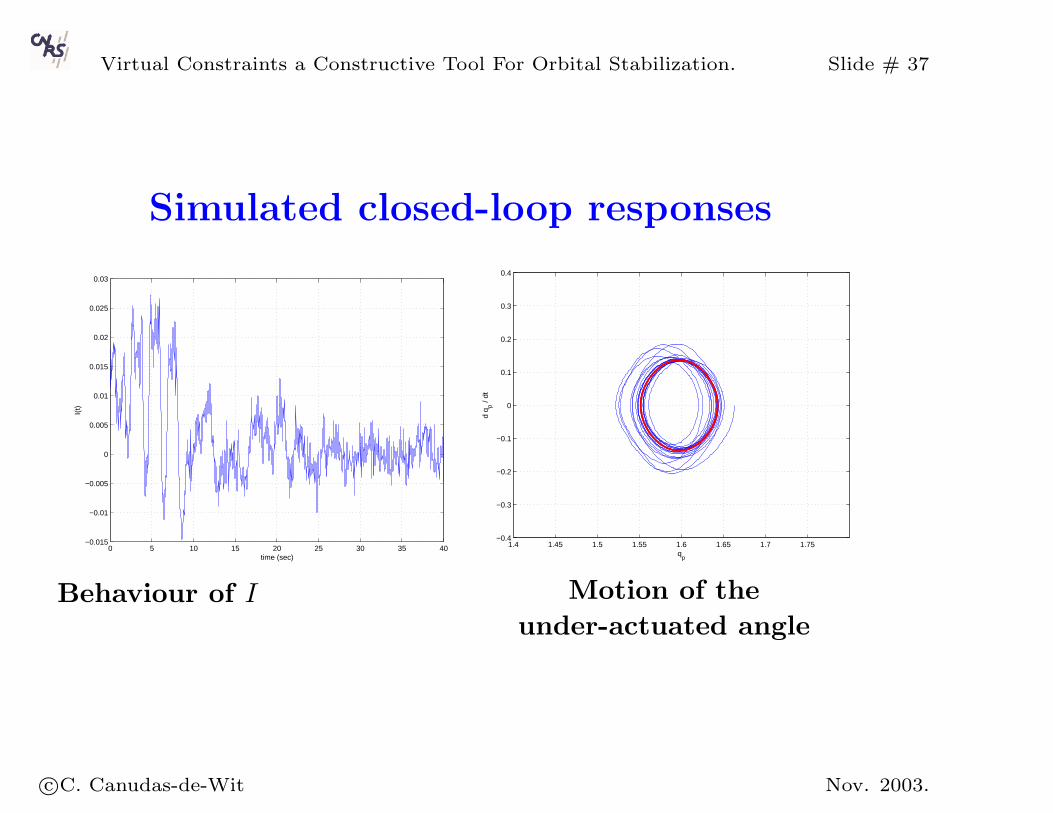
Simulated closed-loop responses
0 5 10 15 20 25 30 35 40−0.015
−0.01
−0.005
0
0.005
0.01
0.015
0.02
0.025
0.03
time (sec)
I(t)
Behaviour of I
1.4 1.45 1.5 1.55 1.6 1.65 1.7 1.75−0.4
−0.3
−0.2
−0.1
0
0.1
0.2
0.3
0.4
qp
d q p /
dt
Motion of theunder-actuated angle
c©C. Canudas-de-Wit Nov. 2003.
Virtual Constraints a Constructive Tool For Orbital Stabilization. Slide # 38
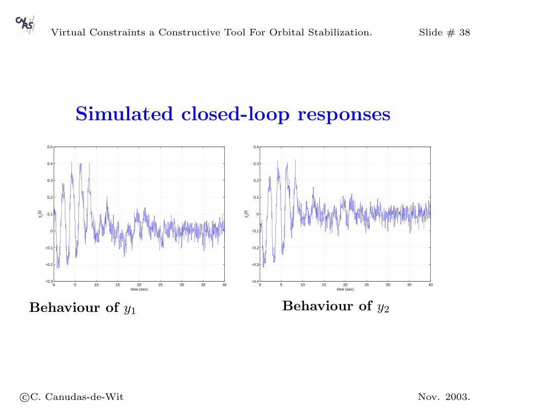
Simulated closed-loop responses
0 5 10 15 20 25 30 35 40−0.3
−0.2
−0.1
0
0.1
0.2
0.3
0.4
0.5
time (sec)
y 1(t)
Behaviour of y1
0 5 10 15 20 25 30 35 40−0.4
−0.3
−0.2
−0.1
0
0.1
0.2
0.3
0.4
time (sec)
y 2(t)
Behaviour of y2
c©C. Canudas-de-Wit Nov. 2003.
Virtual Constraints a Constructive Tool For Orbital Stabilization. Slide # 39
References
[1] Aracil, J. Gomez-Estern, F. and Gordillo, F. (2003)“A Family of
oscillating generalized Hamiltonian Systems”. IFAC workshop on
Hamiltonian Systems, Sevilla, April, 2003.
[2] Aracil, Gordillo, F. and Acosta, J.(2002) “Stabilization of oscillations in
the inverted pendulum”. IFAC word Congress. , Barcelona, Spain, Jully,
2002
[3] C. Chevallereau, G. Abba, Y. Aoustin, F. Plestan, E.R. Westervelt, C.
Canudas-de Wit, and J.W. Grizzle.“A Testbed for Advanced Control
Theory”. to appear in: IEEE Control Systems Magazine, Dec. 2003.
[4] Vivas-Venegas, C. and Rubio, F.(2003) “Improving the performance of
orbitally-stabilizing controls for the furuta pendulum ”. IFAC workshop
on Hamiltonian Systems, Sevilla, April, 2003.
[5] Grognard, F. and C. Canudas-de-Wit (2002) “Design of orbitally stable
zero-dynamics for a class of nonlinear systems,”. In Proceeding of the
IEEE Decision and Control Conference, Dec. 2002 Las Vegas, Nevada,
USA. Also to apprear in: Systems & Control Letters.
[6] Hauser, J. and C.C. Chung (1994). Converse Lyapunov functions for
c©C. Canudas-de-Wit Nov. 2003.
Virtual Constraints a Constructive Tool For Orbital Stabilization. Slide # 40
exponentially stable periodic orbits. Systems & Control Letters
(23), 27–34.
[7] Canudas de Wit C., Espiau B., Urrea C. (2002), “Orbital stabilization of
underactuated mechanical systems,” IFAC word Congress, 2002,
Barcelona, Spain.
[8] Marconi L., Isidori A., Sarrani A., “Autonomous vertical landing on an
oscillating platform: an internal-model based approach,” Automatica 38
(2002), no. 1, 21-32.
[9] Perram J., Shiriaev A., Canudas-de-Wit C., Grognard F. “Explicit
Formula for A General Integral Of Motion For A Class Of Mechanical
Systems Subject To Holonomic Constraint”. IFAC workshop on
Hamiltonian Systems, Sevilla, April, 2003.
[10] Shiriaev A. and Canudas-de-Wit “Virtual Constraints a constructive tool
for orbital stabilisation of underacutaed nonlinear systems: theory and
examples”. Paper in two parts. Submitted to IEEE Trans. on Aut.
Control, Nov. 2003.
c©C. Canudas-de-Wit Nov. 2003.