NONLINEAR VISCOSITY Linear, isotropic, …...NONLINEAR VISCOSITY Linear, isotropic,incompressible, viscous fluid. A fluid deforms in a homogeneous state, with stress σ ij and rate

Plasticity http://imechanica.org/node/17162 Z. Suo

October 13, 2014 Nonlinear viscosity 1

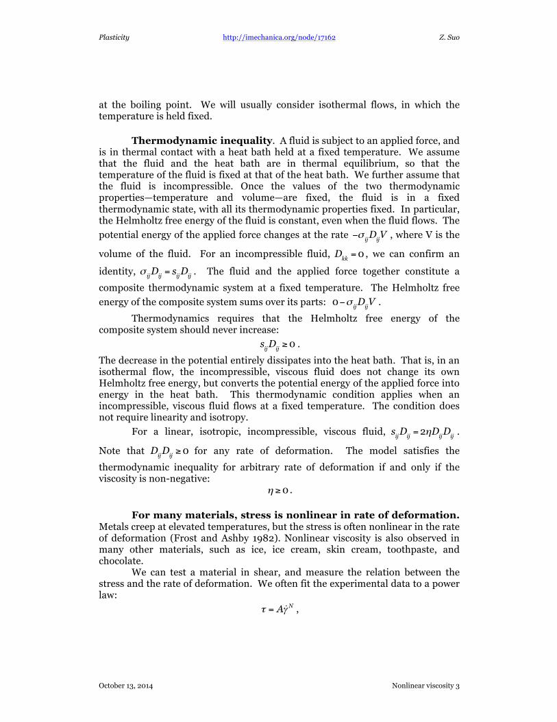
NONLINEAR VISCOSITY Linear, isotropic, incompressible, viscous fluid. A fluid deforms

in a homogeneous state, with stress σij

and rate of deformation Dij

. The mean

stress is σm=σ

kk/3 , and the deviatoric stress is s

ij=σ

ij−σ

mδij

. By a linear,

isotropic, incompressible, viscous fluid we mean a model specified by

Dkk=0 ,

sij=2ηD

ij,

where η is the viscosity. The model assumes that η is independent of the rate of deformation, so

that the deviatoric stress is linear in the rate of deformation. The expression

Dkk=0 ensures incompressibility, and represents a single equation:

D11+D

22+D

33=0 .

The expression sij=2ηD

ij ensures isotropy, and represents six equations:

σ12=2ηD

12,

σ23=2ηD

23,

σ31=2ηD

31,

σ11−σ11+σ

22+σ

33

3=2ηD

11,

σ22−σ22+σ

33+σ

11

3=2ηD

22,

σ33−σ33+σ

11+σ

22

3=2ηD

33.

The sum of the last three equations gives an identity, 0 = 0. Thus, the last three equations consist of only two independent equations.

The two types of relations, Dkk=0 and s

ij=2ηD

ij, consist of a total of six

independent linear equations between the twelve components of stress and rate of deformation. Thermodynamic state and thermodynamic property. A fluid can be in many thermodynamic states, and has many thermodynamic properties. Examples of thermodynamic properties include temperature, pressure, volume, energy, entropy, smell, color, electric field, and polarization. When the fluid is in a particular thermodynamic state, the value of every thermodynamic property is fixed. We specify a thermodynamic state of a fluid by values of its thermodynamic properties.



How many thermodynamic properties do we need to differentiate thermodynamic states of a fluid? The answer is two. How do we know? The answer depends on the evidence from our experience and on the limit of our attention. One property is too few: if we hold the value of the temperature we can still change the thermodynamic state of the fluid by changing the pressure. Three properties are too many: once the temperature and pressure are fixed, the thermodynamic state of the fluid is fixed if we neglect minor effects of, say, the electric field and magnetic field. As a model, we specify the thermodynamic state using two thermodynamic properties, for example, temperature and pressure. Once the values of the two thermodynamic properties are fixed, the fluid is in a fixed thermodynamic state, and values of all other thermodynamic properties are fixed. In this model, the deviatoric stress is not a thermodynamic property, and does not affect thermodynamic state of the fluid. Viscosity is a thermodynamic property. The viscosity of a fluid is a

function of temperature and pressure, η T ,p( ) . The experimental data are

sometimes fit to an expression

η T ,p( ) =η0 expq+V

ap

kT

!

"##

$

%&& .

Here kT is the temperature in the unit of energy; the pre-factor η0

, the activation

energy q and the activation volume Va

are parameters used to fit the

experimental data. The model also requires that the mean stress equal the thermodynamic pressure:

σ11+σ

22+σ

33

3= p .

The pressure-dependent viscosity makes the model of viscosity, sij=2ηD

ij,

nonlinear. Is this nonlinear effect significant? At room temperature,

kT = 1.38×10−23J/K( ) 300K( ) = 4×10−21 J . Assume that the activation volume is

comparable to the volume per molecule, Va≈ 3×10−29m3 , and assume a value of

pressure p = 106Pa . We find that Vap << kT . Thus, in many applications, the

effect of pressure on viscosity is small, so that the viscosity is assumed to be independent of the pressure. Often the activation energy is large, q >> kT , and the viscosity is sensitive to temperature. At the atmospheric pressure, the viscosity of water is around 10-3

Pa.s at room temperature, 1.8×10−3 Pa.s at the freezing point, and 0.28×10−3 Pa.s



at the boiling point. We will usually consider isothermal flows, in which the temperature is held fixed. Thermodynamic inequality. A fluid is subject to an applied force, and is in thermal contact with a heat bath held at a fixed temperature. We assume that the fluid and the heat bath are in thermal equilibrium, so that the temperature of the fluid is fixed at that of the heat bath. We further assume that the fluid is incompressible. Once the values of the two thermodynamic properties—temperature and volume—are fixed, the fluid is in a fixed thermodynamic state, with all its thermodynamic properties fixed. In particular, the Helmholtz free energy of the fluid is constant, even when the fluid flows. The

potential energy of the applied force changes at the rate −σijDijV , where V is the

volume of the fluid. For an incompressible fluid, Dkk=0 , we can confirm an

identity, σijDij= s

ijDij

. The fluid and the applied force together constitute a

composite thermodynamic system at a fixed temperature. The Helmholtz free

energy of the composite system sums over its parts: 0−σijDijV .

Thermodynamics requires that the Helmholtz free energy of the composite system should never increase:

sijDij≥0 .

The decrease in the potential entirely dissipates into the heat bath. That is, in an isothermal flow, the incompressible, viscous fluid does not change its own Helmholtz free energy, but converts the potential energy of the applied force into energy in the heat bath. This thermodynamic condition applies when an incompressible, viscous fluid flows at a fixed temperature. The condition does not require linearity and isotropy.

For a linear, isotropic, incompressible, viscous fluid, sijDij=2ηD

ijDij

.

Note that DijDij≥0 for any rate of deformation. The model satisfies the

thermodynamic inequality for arbitrary rate of deformation if and only if the viscosity is non-negative: η ≥0 . For many materials, stress is nonlinear in rate of deformation. Metals creep at elevated temperatures, but the stress is often nonlinear in the rate of deformation (Frost and Ashby 1982). Nonlinear viscosity is also observed in many other materials, such as ice, ice cream, skin cream, toothpaste, and chocolate. We can test a material in shear, and measure the relation between the stress and the rate of deformation. We often fit the experimental data to a power law:

τ = A γ N ,



where A and N are parameters used to fit the experimentally measured curve between the stress and the rate of deformation. The power law is also written as

γ = τA

!

"#

$

%&

n

,

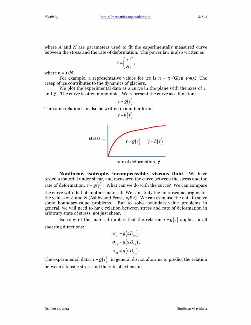
where n = 1/N. For example, a representative values for ice is n = 3 (Glen 1955). The creep of ice contributes to the dynamics of glaciers. We plot the experimental data as a curve in the plane with the axes of τ and γ . The curve is often monotonic. We represent the curve as a function:

τ = g γ( ) .

The same relation can also be written in another form:

γ = h τ( ) .

Nonlinear, isotropic, incompressible, viscous fluid. We have tested a material under shear, and measured the curve between the stress and the

rate of deformation, τ = g γ( ) . What can we do with the curve? We can compare

the curve with that of another material. We can study the microscopic origins for the values of A and N (Ashby and Frost, 1982). We can even use the data to solve some boundary-value problems. But to solve boundary-value problems in general, we will need to have relation between stress and rate of deformation in arbitrary state of stress, not just shear.

Isotropy of the material implies that the relation τ = g γ( ) applies in all

shearing directions:

σ12= g 2D

12( ) ,

σ23= g 2D

23( ) ,

σ31= g 2D

31( ) .

The experimental data, τ = g γ( ) , in general do not allow us to predict the relation

between a tensile stress and the rate of extension.

stress, τ

rate of deformation,

γ = h τ( )τ = g γ( )

γ



By viscosity here we mean that the deviatoric stress depends on the rate of deformation. In general we need to determine functions of five independent variables:

sij= s

ijD11,D22,D23,D31,D12( ) .

Here we have dropped the dependence on D33

; due to incompressibility, D33

is

not an independent quantity, D33= −D

11−D

22.

A brute-force method to determine these functions of five variables is to measure them experimentally. This method is impractical. A function of one variable corresponds to a curve, a function of two variables corresponds to many curves on a page, a function of three variables corresponds to many pages of a book, and a function of four variables corresponds to many books in a library. A function of five variables will require many libraries. We need to construct a model to reduce the number of experiments. We wish to modify the multiaxial model of viscosity in a single aspect. The new model will accommodate the nonlinear relation between stress and rate of deformation, but will preserve incompressibility and isotropy. The condition of incompressibility remains the same:

Dkk=0 .

We need to learn how to preserve isotropy.

Invariant of a vector. Let e1,e2,e3

be an orthonormal basis of a

Euclidean space. Any vector u in the Euclidean space is a linear combination of the base vectors:

u = u1e1+u

2e2+u

3e3

.

We say that u1,u2,u3

are the components of the vector u relative to the basis

e1,e2,e3

. We are familiar with the geometric interpretations of these ideas. The

vector u is an arrow in the space. The basis e1,e2,e3

consists of three unit

vectors normal to one another. The components u1,u2,u3

are the projection of

the vector u on to the three unit vectors e1,e2,e3

.

Once a vector u is given in the Euclidean space, the vector itself does not

change if we choose another basis. However, the components u1,u2,u3

do change

if we choose another basis. We know the rule of the transformation of the components of the same vector relative to two bases.

The sum uiui does not have any free index, and is a scalar. When a new

basis is used, the components u1,u2,u3

change, but uiui remains invariant. This

invariant has a familiar geometric interpretation: uiui

is the length of the

vector u. The length of the vector is invariant when the basis changes.



Invariants of a tensor. Let A be a second-rank tensor, and Aij

be the

components of the tensor relative to an orthonormal basis e1,e2,e3

. The tensor

is symmetric, so that Aij= A

ji. The components of the tensor form three scalars:

Aii, A

ijAij, A

ijAjkAki

.

We form a scalar by combining the components of the tensor in a way that makes all indices dummy. The three scalars are independent of the choice of the basis

e1,e2,e3

, and are known as the invariants of the tensor A.

Invariants of stress tensor. The state of stress is a physical fact,

independent of how we choose a basis. Once we choose a basis e1,e2,e3

, we

picture a unit cube in the fluid, with the faces of the cube on the coordinate planes. Forces acting on the faces of the cube define the components of the

stress, σij

, relative to the basis. Whereas the state of stress does not depend on

the choice of the basis, the components of the stress do. Some combinations of the components are invariants, independent of the

choice of basis. For example, the trace of the stress tensor, σkk

, is an invariant.

The flow of an incompressible fluid is unaffected when we superimpose any

hydrostatic stress. Define the deviatoric stress, sij=σ

ij−σ

kkδij/3 , and write the

other two invariants of the stress tensor as

sijsij, s

ijsjkski

.

Each invariant is a scalar measure of the state of stress. The two invariants are

sometimes designated as J2= s

ijsij/2 and J

3= s

ijsjkski/3 .

Invariants of rate-of-deformation tensor. For an incompressible material, the trace of the deformation gradient vanishes,

Dkk=0 .

We write the other two invariants of the rate of deformation as

DijDij

, DijDjkDki

.

Each invariant is a scalar measure of the rate of deformation. The two invariants

are sometimes designated as I2=D

ijDij/2 and I

3=D

ijDjkDki/3 .

The second-invariant fluid. We have tested a fluid under shear, and

measured the curve between the stress and the rate of deformation, τ = g γ( ) .

Can we use this curve to predict the curve between the stress and the rate of deformation under all other states of stress? The answer is no. However we



fudge the prediction, it will disagree with the experimental data for some states of

stress. But the desire to use the curve τ = g γ( ) to predict the curves between

stress and rate of deformation for all states of stress is so strong that we do it by making assumptions. Fudge we do. The most widely used model relies on the second invariant of the rate of deformation. The model makes two assumptions. First, the relation between the stress and the rate of deformation takes the form:

Dkk=0 ,

sij=2ηD

ij.

Second, the viscosity η varies with the rate of deformation in a particular way—

the viscosity is a function of the second invariant, η DijDij( ) . The use of the

invariant preserves isotropy. The use of only one invariant simplifies the model.

The model ensures incompressibility. Once we know the function η DijDij( ) , the

model calculates all components of the deviatoric stress for any given rate of deformation. Fit the second-invariant model to experimental data. Recall that γ12=2D

12. When the fluid flows in shear, the second-invariant model s

ij=2ηD

ij

predicts that σ12=η γ

12. Comparing this prediction to the experimental data

τ = g γ( ) , we obtain that

η =g γ( )γ

.

To make the model applicable to general state of deformation, we need to convert the independent variable from the rate of shear to the second invariant. Under the pure shear condition, the second invariant is

DijDij=D

12D12+D

21D21=12γ 2 .

Define the equivalent rate of shear by

γe= 2D

ijDij

.

The second invariant DijDij

is positive-definite. The equivalent rate of shear is

just another way to write the second invariant. Write

η γe( ) =g γ

e( )γe

.

We have just described the most commonly used model of nonlinear, isotropic, incompressible viscosity. We summarize the model as a recipe.



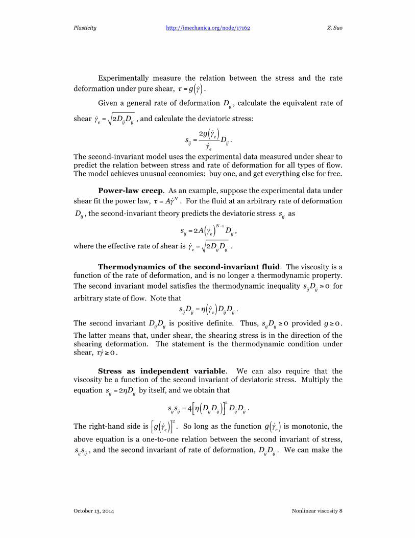
Experimentally measure the relation between the stress and the rate

deformation under pure shear, τ = g γ( ) .

Given a general rate of deformation Dij

, calculate the equivalent rate of

shear γe= 2D

ijDij

, and calculate the deviatoric stress:

sij=2g γ

e( )γe

Dij

.

The second-invariant model uses the experimental data measured under shear to predict the relation between stress and rate of deformation for all types of flow. The model achieves unusual economics: buy one, and get everything else for free. Power-law creep. As an example, suppose the experimental data under

shear fit the power law, τ = A γ N . For the fluid at an arbitrary rate of deformation

Dij

, the second-invariant theory predicts the deviatoric stress sij

as

sij=2A γ

e( )N−1Dij

,

where the effective rate of shear is γe= 2D

ijDij

.

Thermodynamics of the second-invariant fluid. The viscosity is a function of the rate of deformation, and is no longer a thermodynamic property.

The second invariant model satisfies the thermodynamic inequality sijDij≥0 for

arbitrary state of flow. Note that

sijDij=η γ

e( )DijDij . The second invariant D

ijDij

is positive definite. Thus, sijDij≥0 provided g≥0 .

The latter means that, under shear, the shearing stress is in the direction of the shearing deformation. The statement is the thermodynamic condition under shear, τ γ ≥0 . Stress as independent variable. We can also require that the viscosity be a function of the second invariant of deviatoric stress. Multiply the

equation sij=2ηD

ij by itself, and we obtain that

sijsij= 4 η D

ijDij( )!

"#$2

DijDij

.

The right-hand side is g γe( )!

"#$2

. So long as the function g γe( ) is monotonic, the

above equation is a one-to-one relation between the second invariant of stress,

sijsij

, and the second invariant of rate of deformation, DijDij

. We can make the



viscosity as a function of the second invariant of the deviatoric stress, η sijsij( ) .

The second-invariant model is also known as the J2 model. Under the pure shear condition, the deviatoric stress is

sij

!"

#$=

0 τ 0τ 0 00 0 0

!

"

%%%

#

$

&&&

.

The second invariant is

sijsij= s12s12+ s21s21=2τ 2 .

Define the equivalent shear by

τe=12sijsij

.

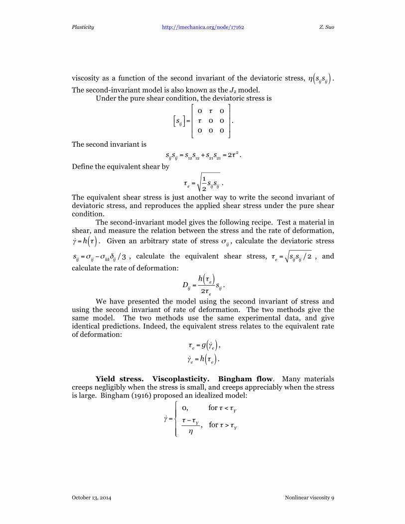
The equivalent shear stress is just another way to write the second invariant of deviatoric stress, and reproduces the applied shear stress under the pure shear condition. The second-invariant model gives the following recipe. Test a material in shear, and measure the relation between the stress and the rate of deformation, γ = h τ( ) . Given an arbitrary state of stress σ

ij, calculate the deviatoric stress

sij=σ

ij−σ

kkδij/3 , calculate the equivalent shear stress, τ

e= s

ijsij/2 , and

calculate the rate of deformation:

Dij=h τ

e( )2τe

sij

.

We have presented the model using the second invariant of stress and using the second invariant of rate of deformation. The two methods give the same model. The two methods use the same experimental data, and give identical predictions. Indeed, the equivalent stress relates to the equivalent rate of deformation:

τe= g γ

e( ) ,

γe= h τ

e( ) .

Yield stress. Viscoplasticity. Bingham flow. Many materials creeps negligibly when the stress is small, and creeps appreciably when the stress is large. Bingham (1916) proposed an idealized model:

γ =0, for τ < τ

Y

τ −τY

η, for τ > τ

Y

"

#$$

%$$



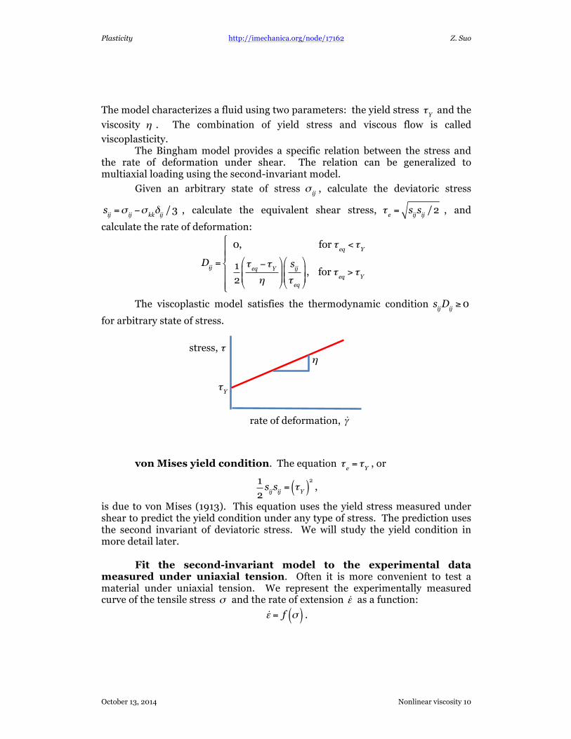
The model characterizes a fluid using two parameters: the yield stress τY

and the

viscosity η . The combination of yield stress and viscous flow is called

viscoplasticity. The Bingham model provides a specific relation between the stress and the rate of deformation under shear. The relation can be generalized to multiaxial loading using the second-invariant model.

Given an arbitrary state of stress σij

, calculate the deviatoric stress

sij=σ

ij−σ

kkδij/3 , calculate the equivalent shear stress, τ

e= s

ijsij/2 , and

calculate the rate of deformation:

Dij=

0, for τeq< τ

Y

12

τeq−τ

Y

η

"

#$$

%

&''sij

τeq

"

#$$

%

&'', for τ eq > τY

(

)**

+**

The viscoplastic model satisfies the thermodynamic condition sijDij≥0

for arbitrary state of stress.

von Mises yield condition. The equation τe= τ

Y, or

12sijsij= τ

Y( )2

,

is due to von Mises (1913). This equation uses the yield stress measured under shear to predict the yield condition under any type of stress. The prediction uses the second invariant of deviatoric stress. We will study the yield condition in more detail later. Fit the second-invariant model to the experimental data measured under uniaxial tension. Often it is more convenient to test a material under uniaxial tension. We represent the experimentally measured curve of the tensile stress σ and the rate of extension ε as a function:

ε = f σ( ) .

stress, τ

rate of deformation, γ

τY

η



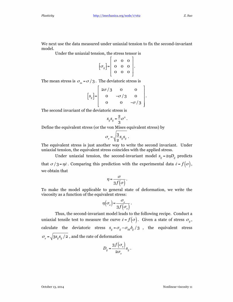
We next use the data measured under uniaxial tension to fix the second-invariant model. Under the uniaxial tension, the stress tensor is

σij

!"

#$=

σ 0 00 0 00 0 0

!

"

%%%

#

$

&&&

.

The mean stress is σm=σ /3 . The deviatoric stress is

sij

!"

#$=

2σ /3 0 0

0 −σ /3 0

0 0 −σ /3

!

"

&&&&

#

$

''''

.

The second invariant of the deviatoric stress is

sijsij=23σ 2 .

Define the equivalent stress (or the von Mises equivalent stress) by

σe=32sijsij

.

The equivalent stress is just another way to write the second invariant. Under uniaxial tension, the equivalent stress coincides with the applied stress.

Under uniaxial tension, the second-invariant model sij=2ηD

ij predicts

that σ /3=η ε . Comparing this prediction with the experimental data ε = f σ( ) ,

we obtain that

η =σ

3 f σ( ).

To make the model applicable to general state of deformation, we write the viscosity as a function of the equivalent stress:

η σe( ) = σ

e

3 f σe( )

.

Thus, the second-invariant model leads to the following recipe. Conduct a

uniaxial tensile test to measure the curve ε = f σ( ) . Given a state of stress σij

,

calculate the deviatoric stress sij=σ

ij−σ

kkδij/3 , the equivalent stress

σe= 3s

ijsij/2 , and the rate of deformation

Dij=3 f σ

e( )2σ

e

sij

.



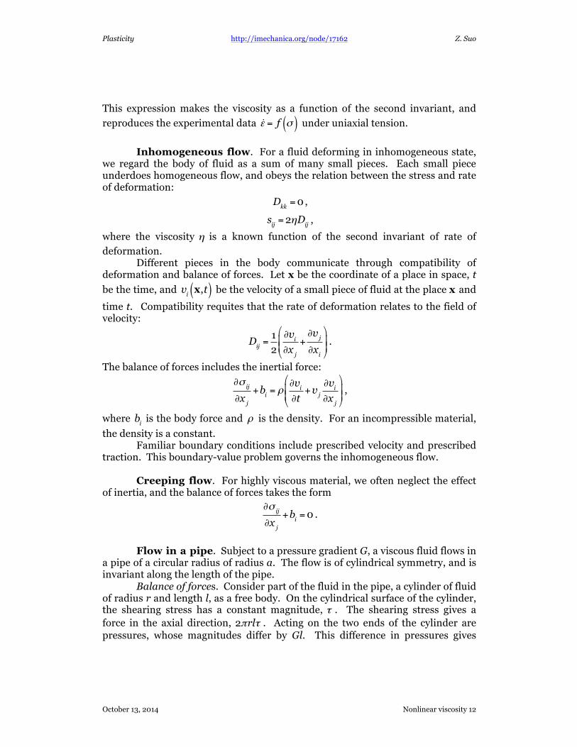
This expression makes the viscosity as a function of the second invariant, and

reproduces the experimental data ε = f σ( ) under uniaxial tension.

Inhomogeneous flow. For a fluid deforming in inhomogeneous state, we regard the body of fluid as a sum of many small pieces. Each small piece underdoes homogeneous flow, and obeys the relation between the stress and rate of deformation:

Dkk=0 ,

sij=2ηD

ij,

where the viscosity η is a known function of the second invariant of rate of

deformation. Different pieces in the body communicate through compatibility of deformation and balance of forces. Let x be the coordinate of a place in space, t

be the time, and vix,t( ) be the velocity of a small piece of fluid at the place x and

time t. Compatibility requites that the rate of deformation relates to the field of velocity:

Dij=12

∂vi

∂xj

+∂vj

∂xi

"

#$$

%

&'' .

The balance of forces includes the inertial force:

∂σ

ij

∂xj

+bi= ρ

∂vi

∂t+v

j

∂vi

∂xj

"

#$$

%

&'' ,

where bi is the body force and ρ is the density. For an incompressible material,

the density is a constant. Familiar boundary conditions include prescribed velocity and prescribed traction. This boundary-value problem governs the inhomogeneous flow. Creeping flow. For highly viscous material, we often neglect the effect of inertia, and the balance of forces takes the form

∂σ

ij

∂xj

+bi=0 .

Flow in a pipe. Subject to a pressure gradient G, a viscous fluid flows in a pipe of a circular radius of radius a. The flow is of cylindrical symmetry, and is invariant along the length of the pipe. Balance of forces. Consider part of the fluid in the pipe, a cylinder of fluid of radius r and length l, as a free body. On the cylindrical surface of the cylinder, the shearing stress has a constant magnitude, τ . The shearing stress gives a force in the axial direction, 2πrlτ . Acting on the two ends of the cylinder are pressures, whose magnitudes differ by Gl. This difference in pressures gives



another force in the axial direction, πr2Gl . The balance of the two axial forces,

2πrlτ = πr2Gl , gives that

τ =12Gr .

Thus, the shearing stress is linear in the radial distance. Compatibility of deformation. The velocity field of the fluid particles

directs in the axial direction, and varies with the radial distance, v r( ) . We

assume fluid at the surface of the pipe does not slip, v a( ) =0 . The gradient of

velocity gives the rate of shear, γ = dv /dr . Integrating, we obtain that

v r( ) = γ r( )dra

r

∫ .

The rate of discharge is

Q = v r( )2πrdr0

a

∫ .

Rheology of fluid. We model the fluid by a nonlinear relation between rate of shear γ and shearing stress.

γ = h τ( ) .

Mixing the three ingredients. The three ingredients relate the rate of discharge Q to the gradient of pressure G. First consider a linearly viscous fluid. Tested under shear, the rate of deformation relates to the stress as γ = τ /η , with η being a constant. Because the shearing stress is linear in radial distance,

τ =Gr /2 , the rate of shear is also linear in radial distance,

γ = Gr2η

.

The velocity is quadratic in the radial distance:

v r( ) = G4ηr2 −a2( ) .


Q =πa4G8η

.

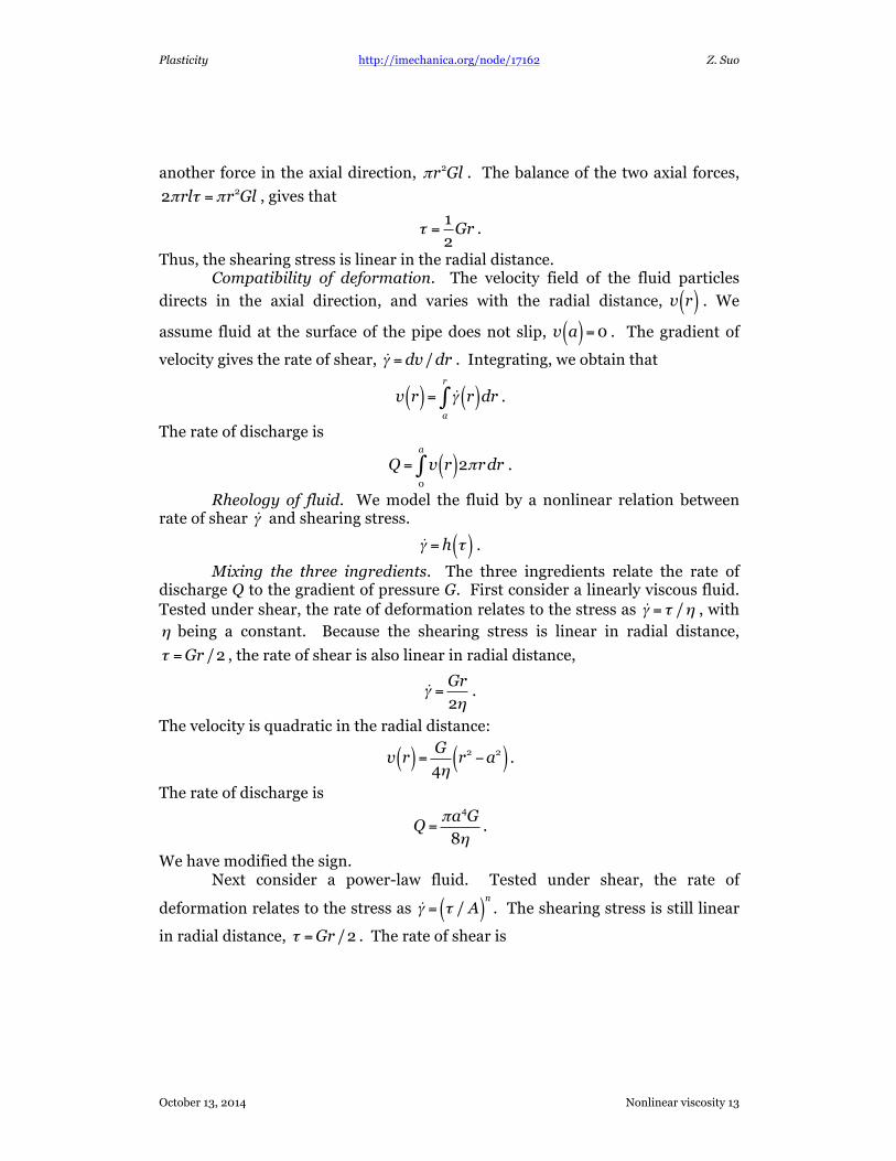
We have modified the sign. Next consider a power-law fluid. Tested under shear, the rate of

deformation relates to the stress as γ = τ / A( )n

. The shearing stress is still linear

in radial distance, τ =Gr /2 . The rate of shear is



γ = Gr2A

!

"#

$

%&

n

.

The velocity is

v r( ) = G2A

!

"#

$

%&

nrn+1 −an+1

n+1.


Q =Ga2A

!

"#

$

%&

nπa3

n+3.

Growth of a cavity. An incompressible material in a state of

hydrostatic stress σappl

does not deform. However, the material will deform if it

contains a cavity. We neglect the surface energy of the cavity, and assume that the cavity is traction-free. Consequently, near the cavity the material is not in a state of hydrostatic stress. Far away from the cavity, the material is still in the

state of hydrostatic stress σappl

. This applied stress will cause the cavity to

enlarge. We assume the cavity to be spherical, so that the non-vanishing fields are

the radial component of stress σr, circumferential components of stress σ

θ, and

the radial component of the velocity v. For the cavity at a given radius a, all these fields are functions of radial coordinate r. Balance of forces. Consider a hemispherical shell, inner radius r and outer radius r + dr, cut from a spherical shell with a plane normal to the z axis.

The radial stress on the outer surface of the shell is σrr+dr( ) , resulting in a force

in the positive z direction, π r+dr( )2σrr+dr( ) . The radial stress on the inner

surface is σrr( ) , resulting in a force in the negative z direction, πa2σ

rr( ) . The

base of the hemispherical shell is a circular annulus, and the circumferential

stress gives a force in the negative z direction, 2πrdr( )σθr( ) . Balancing these

forces acting on the hemispherical shell, we obtain that

dσ

r

dr+2rσr−σ

θ( ) =0 .

Compatibility of deformation. Denote the radius of cavity at time t by

a t( ) . At a given time, the velocity of the surface of the cavity is v a( ) = da /dt , and

the volume of material per unit time crossing the surface of the cavity is

4πa2 da /dt( ) . The volume of material per unit time crossing the spherical



surface of radius r is 4πr2v r( ) . Incompressibility of the material requires that

the two flows be equal, 4πr2v r( ) = 4πa2 da /dt( ) , giving the velocity field:

v r( ) = a2

r2dadt

.

The velocity decays as a function of the distance r. The rate of deformation in the

radial direction is Dr= dv /dr , or

Dr= −2a2

r3dadt

.

The rates of deformation in the circumferential directions are Dθ= v /r . The

material contacts in the radial direction and extends in the circumferential directions. Rheology of material. Consider a nonlinear, viscous material. Tested under uniaxial tensile stress, the stress relates to the rate of deformation as

σ = f ε( ) .

Each small piece of material around the cavity is in a state of triaxial stress,

σr,σ

θ,σ

θ( ) , and a state of triaxial rate of deformation, Dr,−D /2

r,−D

r/2( ) .

Superimposing a state of hydrostatic stress does not affect the flow. Superposing

a state of hydrostatic stress −σθ,−σ

θ,−σ

θ( ) on the original state σr,σ

θ,σ

θ( ) , we

obtain a state of uniaxial compressive stress, σr−σ

θ,0,0( ) , and keep the state of

deformation the same, Dr,−D /2

r,−D

r/2( ) . We assume that the rheological

model is symmetric with respect to tension and compression. In the relation

σ = f ε( ) , we replace σ with − σr−σ

θ( ) , and ε with −Dr, so that

− σr−σ

θ( ) = f −Dr( ) .

Mixing the three ingredients. Consider a power-law material, σ = K ε( )N

.

Replacing σ with − σr−σ

θ( ) , and ε with −Dr, we obtain that

σθ−σ

r= K

2a2

r3dadt

"

#$$

%

&''

N

.

Inserting this expression into the equation for the balance of force, we obtain that

dσ

r

dr=2Kr2a2

r3dadt

!

"##

$

%&&

N

.

Integrating over the interval r ∈ a,∞( ) , and using the boundary conditions

σra( ) =0 and σ

r∞( ) =σ appl , we obtain that



σappl

=2K3N

2adadt

!

"#

$

%&

N

.

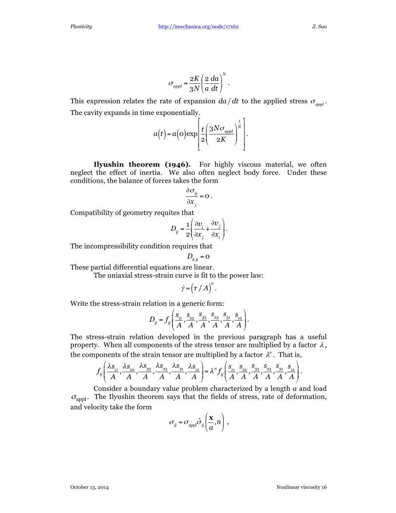
This expression relates the rate of expansion da /dt to the applied stress σappl

.

The cavity expands in time exponentially.

a t( ) = a 0( )exp t2

3Nσappl

2K

!

"##

$

%&&

1N

'

(

)))

*

+

,,,

.

Ilyushin theorem (1946). For highly viscous material, we often neglect the effect of inertia. We also often neglect body force. Under these conditions, the balance of forces takes the form

∂σ

ij

∂xj

=0 .

Compatibility of geometry requites that

Dij=12

∂vi

∂xj

+∂vj

∂xi

"

#$$

%

&'' .

The incompressibility condition requires that

Dk ,k=0

These partial differential equations are linear. The uniaxial stress-strain curve is fit to the power law:

γ = τ / A( )n

.

Write the stress-strain relation in a generic form:

Dij= f

ij

s11

A,s22

A,s33

A,s23

A,s31

A,s12

A

!

"##

$

%&& .

The stress-strain relation developed in the previous paragraph has a useful property. When all components of the stress tensor are multiplied by a factor λ , the components of the strain tensor are multiplied by a factor nλ . That is,

fij

λs11

A,λs22

A,λs33

A,λs23

A,λs31

A,λs12

A

!

"##

$

%&&= λ

n fij

s11

A,s22

A,s33

A,s23

A,s31

A,s12

A

!

"##

$

%&& .

Consider a boundary value problem characterized by a length a and load σappl . The Ilyushin theorem says that the fields of stress, rate of deformation,

and velocity take the form

σij=σ

applσ̂ij

xa,n

!

"#

$

%& ,



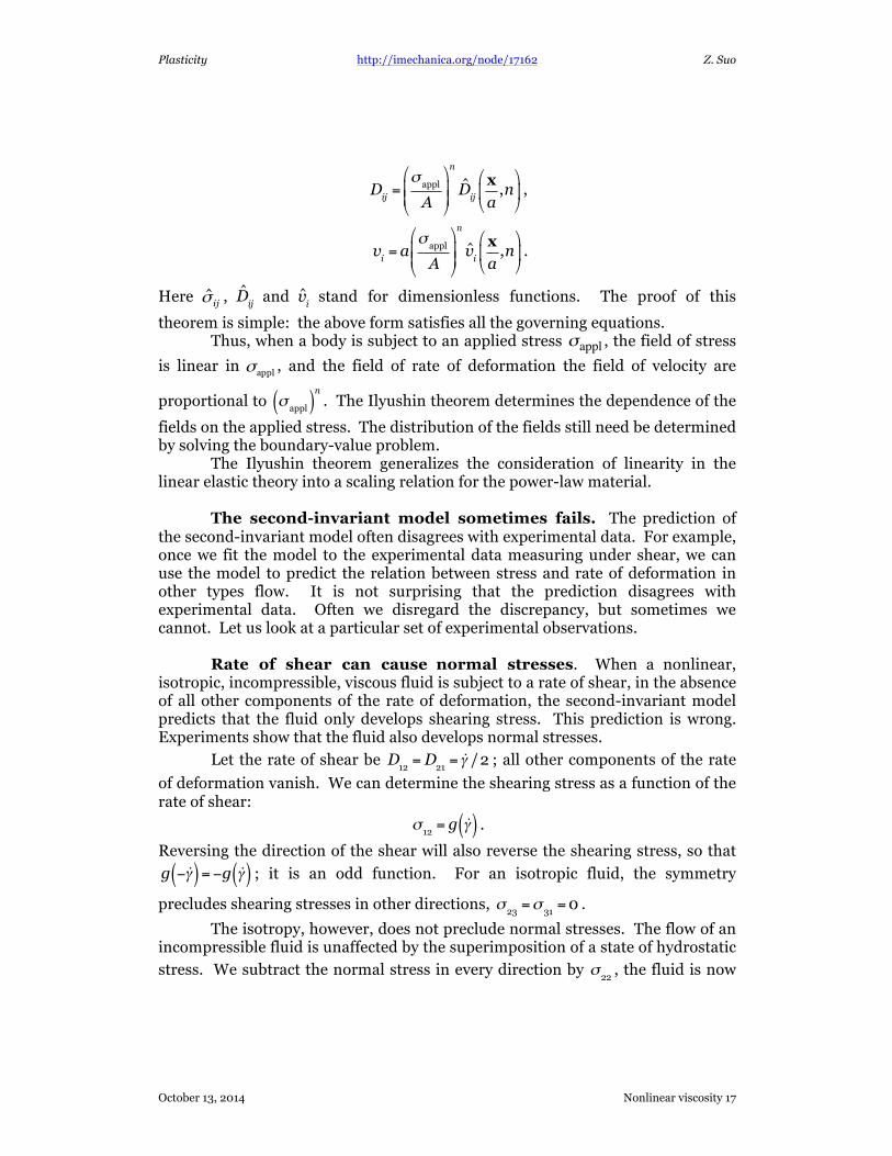
Dij=σappl

A

!

"##

$

%&&

n

D̂ij

xa,n

!

"#

$

%& ,

vi= a

σappl

A

!

"##

$

%&&

n

v̂i

xa,n

!

"#

$

%& .

Here ijσ̂ , D̂ij

and v̂i

stand for dimensionless functions. The proof of this

theorem is simple: the above form satisfies all the governing equations. Thus, when a body is subject to an applied stress σappl , the field of stress

is linear in applσ , and the field of rate of deformation the field of velocity are

proportional to σappl( )

n. The Ilyushin theorem determines the dependence of the

fields on the applied stress. The distribution of the fields still need be determined by solving the boundary-value problem. The Ilyushin theorem generalizes the consideration of linearity in the linear elastic theory into a scaling relation for the power-law material. The second-invariant model sometimes fails. The prediction of the second-invariant model often disagrees with experimental data. For example, once we fit the model to the experimental data measuring under shear, we can use the model to predict the relation between stress and rate of deformation in other types flow. It is not surprising that the prediction disagrees with experimental data. Often we disregard the discrepancy, but sometimes we cannot. Let us look at a particular set of experimental observations. Rate of shear can cause normal stresses. When a nonlinear, isotropic, incompressible, viscous fluid is subject to a rate of shear, in the absence of all other components of the rate of deformation, the second-invariant model predicts that the fluid only develops shearing stress. This prediction is wrong. Experiments show that the fluid also develops normal stresses.

Let the rate of shear be D12=D

21= γ /2 ; all other components of the rate

of deformation vanish. We can determine the shearing stress as a function of the rate of shear:

σ12= g γ( ) .

Reversing the direction of the shear will also reverse the shearing stress, so that

g − γ( ) = −g γ( ) ; it is an odd function. For an isotropic fluid, the symmetry

precludes shearing stresses in other directions, σ23=σ

31=0 .

The isotropy, however, does not preclude normal stresses. The flow of an incompressible fluid is unaffected by the superimposition of a state of hydrostatic

stress. We subtract the normal stress in every direction by σ22

, the fluid is now



subject to normal stress σ11−σ

22 in direction 1, and normal stress σ

33−σ

22 in

direction 3. The two normal stresses are also functions of the rate of shear:

σ11−σ

22= N

1γ( ) ,

σ22−σ

33= N

2γ( ) ,

Reversing the direction of the shear will not affect the normal stresses, so that

N1− γ( ) = N1 γ( ) and N

2− γ( ) = N2 γ( ) ; they are even functions. Experiments show

that the normal stress effects are pronounced in viscoelastic liquids; the first normal stress difference is larger in magnitude than the second normal stress difference (Barnes, Hutton, Walters 1989).

Reiner-Rivlin fluid. In the second invariant model, sij=2ηD

ij, the

viscosity is taken to be a function of the second invariant. We can of course assume that the viscosity is a function of second and third invariants,

η DijDij,DijDjkDki( ) . This model is more general, but requires more experimental

data to fit the function. Besides, the two-invariant model still predicts that a rate of shear generates no normal stresses.

A fluid deforms in a homogeneous state, with stress σij

and rate of

deformation Dij

. Assume that the fluid is isotropic, and that the state of stress is

a function of the state of rate of deformation. The most general form of the function is

σij= aδ

ij+bD

ij+cD

ikDkj

,

where a, b and c are functions of the three invariants Dii,DijDij,DijDjkDki

. This

result is due to Reiner (1945) and Rivlin (1948). We further assume that the fluid is incompressible:

Dkk=0 .

Superimposing a hydrostatic stress does not affect the deformation. Let the

mean stress be σm=σ

kk/3 , and the deviatoric stress be s

ij=σ

ij−σ

mδij

. Modify

the above relation between the stress and the rate of deformation as

sij= 2ηD

ij+4ξ D

ikDkj−D

mkDkmδij( ) ,

where η and ξ are functions of the two remaining invariants, DijDij,DijDjkDki

.

Now consider a fluid subject to a rate of shear, D12=D

21= γ /2 , with all

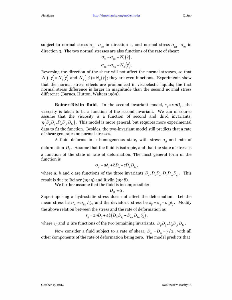
other components of the rate of deformation being zero. The model predicts that



σ12=η γ

σ23=0

σ31=0

σ11−σ11+σ

22+σ

33

3= −ξ γ 2

σ22−σ11+σ

22+σ

33

3= −ξ γ 2

σ33−σ11+σ

22+σ

33

3=2ξ γ 2

The model predicts normal stresses:

σ11−σ

22=0

σ22−σ

33= −3ξ γ 2

This form of normal stresses disagrees with experimental observations. The Reiner-Rivlin model is a general mathematical model of viscosity, but the model does not predict experimentally observed form of normal stresses. Rather, the normal stress effect is pronounced in viscoelastic liquids. Reiner-Rivlin model and the thermodynamic inequality. Let us return to the Reiner-Rivlin model:

σij= aδ

ij+bD

ij+cD

ikDkj

.

The external force does work at the rate

σijDij= aD

kk+bD

ijDij+cD

ikDkjDji

.

For an incompressible fluid, Dkk=0 . The second invariant is nonnegative for all

rates of deformation, DijDij≥0 . The third invariants, however, can be either

positive or negative. If we choose c as a constant, the model will violate the

thermodynamic inequality σijDij≥0 for some rates of deformation. If we choose

the c as c =ζDijDjkDki

with ζ as a positive constant, then the Reiner-Rivlin

model satisfies the thermodynamic inequality for all rates of deformation. Rayleigh’s dissipation function. Rayleigh (1871) introduced the idea of dissipation function in a paper on the vibration of a viscous system. The system has n generalized coordinates. The time derivative of each generalized coordinate defines the associated generalized velocity. Associated with this generalized velocity is a generalized viscous force. Thus, the system has n

generalized velocities, v1,...,v

n, and n generalized viscous forces, f

1,..., f

n. A

general kinetic model is to write each force as a function of the n velocities:



f1v1,...,v

n( )......

fnv1,...,v

n( )

These functions are nonlinear if the viscous behavior is nonlinear. Rayleigh introduced a dissipation function, a scalar function of the

generalized velocities, Q v1,...,v

n( ) . He assumed that the viscous forces take the

form:

fi=∂Q v

1,...,v

n( )∂vi

.

Rayleigh’s kinetic model is more restricted than the general model, but is also simpler. His model only requires a single scalar function of n variables,

Q v1,...,v

n( ) .

Linear viscosity. Rayleigh assumed that the dissipation function is quadratic in the generalized velocities:

Q =12Hijvivj,

where the matrix Hij

represents generalized viscosities. The value of F is

unchanged by the anti-symmetric part of the matrix. We assume that the matrix

is symmetric, Hij=H

ji. The viscous forces are linear in the velocities:

fi=H

ijvj.

We assume that the viscosity of the system dissipates energy,

fivi≥0

for all velocities. The equality holds only when all velocities vanish. In the case

of linear viscosity, fivi=H

ijvivj. The viscosity dissipates energy at all velocities if

and only if the matrix of the viscosity matrix H is positive-definite. When H is nonsingular, we can invert the matrix and obtain

vj=G

ijfi.

The matrix G represents the generalized fluidities. Introduce a scalar

A =12Gijfifj.

This scalar is a function of the viscous forces, A f1,..., f

n( ) , and is called the creep

potential. We confirm that

vi=∂A f

1,... f

n( )∂fi

.



Graphic interpretation of Rayleigh’s kinetic model. We now

generalized Rayleigh’s dissipation function to nonlinear viscosity. Let Q v1,...,v

n( )

be a scalar function of the generalized viscosities, but the function need not be a quadratic in the generalized velocities. Still assume that the viscous forces are given by

fi=∂Q v

1,...,v

n( )∂vi

.

In a linear space of n dimensions, the set of n forces are the components of a vector, and the set of n velocities are the components of another vector. A kinetic model maps one vector to another vector. For a general nonlinear kinetic model,

the map is nonlinear. The function Q v1,...,v

n( ) maps a vector to a scalar. The

gradient of the function maps a vector to a vector. The equation

Q v1,...,v

n( ) = constant

represents a surface in the linear space. The constant is independent of the velocity. At any point on the surface, the gradient of the function is a vector normal to the surface. Rayleigh’s kinetic model specifies that gradient of the

function Q v1,...,v

n( ) gives the force vector. Thus, the force vector is normal to the

surface Q v1,...,v

n( ) = constant.

The inner product of the two vectors, fivi, is power dissipated. For the

power dissipated to be positive definite, the angle between the two vectors must be acute. The shape of the surface is restricted to ensure that the force vector and the velocity vector form an acute angle. Forces as independent variables. Rayleigh’s kinetic model uses the n velocities as independent variables. Alternatively, we can use the n forces as independent variables.

Start with a scalar function of n generalized forces, A f1,..., f

n( ) . For want

of a name different from the dissipation function, let’s call this function of forces the creep potential. Assume that each velocity is the partial derivative of the creep potential with respect to the force associated with the velocity:

vi=∂A f

1,... f

n( )∂fi

.

Legendre transformation. Now we have two kinetic models, one based on a function of velocities, and the other based on a function of forces. Are the two kinetic models the same? Here is the power of mathematics. We can answer this question without worrying whether either kinetic model is useful in the real world. The mathematical idea is as follows.



Start with the model based on a function of n velocities, Q v1,...,v

n( ) . The

forces are given by partial derivatives

fi=∂Q v

1,...,v

n( )∂vi

.

Recall an identify in calculus:

dQ =∂Q v

1,...,v

n( )∂v1

dv1+ ...+

∂Q v1,...,v

n( )∂vn

dvn

.

A comparison of the two expressions gives that

dQ = f1dv1+ ... f

ndvn

.

Next define a new scalar by

A = v1f1+ ...+v

nfn−Q .

According to calculus, this definition leads to

dA = v1df1+ ...+v

ndfn

.

Thus, start with the kinetic model based on the function of n velocities,

Q v1,...,v

n( ) , we obtain n functions of n variables, fiv1,...,v

n( ) . The kinetic model

is said to be invertible if the functions fiv1,...,v

n( ) are one-to-one map between

the set of velocities and the set of forces. For the invertible kinetic model, we can

invert the functions to express velocities in terms of forces, vif1,..., f

n( ) . If the

kinetic model is invertible, the definition of the scalar A ensures that we can

express A as a function of forces, A f1,... f

n( ) . The expression

dA = v1df1+ ...+v

ndfn

tells us that each velocity is a partial derivative of the

function with respected to the force associated with the velocity:

vi=∂A f

1,... f

n( )∂fi

.

This mathematical procedure, known as the Legendre transformation, starts from a function of one set of variables and reaches another function of another set of variables. Apply Rayleigh’s model to construct a nonlinear creep model under multiaxial stress state. Start with a scalar function of stress,

F σ11,...,σ

12( ) . The function maps a tensor to a scalar. Call the function the creep

potential. Assumes that each component of the rate-of-deformation tensor is a partial derivative of the creep potential with respect to the component of stress associated with the component of the rate of deformation:



Dij=∂F σ

11,...,σ

12( )∂σ

ij

For an incompressible, isotropic material, the creep potential is a function

of the two invariants of the deviatoric stress, F J2,J3( ) . For simplicity, we drop

the dependence on J3

and assume that the creep potential is a function of a

single variable, F J3( ) . According to Rayleigh’s kinetic model, the rate of

deformation is

Dij=∂F J

2( )∂σ

ij

=dF J

2( )dJ2

∂J2

∂σij

.

Recall that J2= s

ijsij/2 , so that ∂J

2/∂σ

ij= s

ij. The kinetic model becomes that

Dij=sij

2η,

where η is a function of the second invariant. This procedure recovers the J2

model. References H.A. Barnes, The yield stress. Journal of Non-Newtonian Fluid Mechanics 81,

133-178 (1999). H.A. Barnes, J.F. Hutton, K. Walters. An Introduction to Rheology. Elsevier

1989. E.C. Bingham, Fluidity and Plasticity. McGraw-Hill, 1922. D.V. Boger and K. Walters. Rheological Phenomena in Focus. Elsevier, 1993. B.D. Coleman, H. Markovitz, W. Noll. Viscometric Flows of Non-Newtonian

Fluids. Springer, 1966. H.J. Frost and M.F. Ashby, Deformation-Mechanism Maps: The Plasticity and

Creep of Metals and Ceramics. Pergamon Press, 1982. J.W. Glen, The creep of polycrystalline ice. Proceedings of the Royal Society of

London 228, 519-538 (1955). F. Irgens, Rheology and Non-Newtonian Fluids. Springer, 2014. AA Ilyushin, The theory of small elastic-plastic deformations. Prikadnaia

Matematika i Mekhanika, PMM 10, 347-356 (1946). H. Markovitz, The emergence of rheology. Physics Today 21, 23-30 (1968). E.M. Purcell, Life at low Reynolds number. American Journal of Physics 45, 3-11

(1977). J.W. Strutt (Lord Rayleigh), Some general theorems relating to vibration.

Proceedings of London Mathematical Society s1-4, 357-368 (1871). M. Reiner, A Mathematical Theory of Dilatancy. American Journal of

Mathematics 67, 350-362 (1945).



R.S. Rivlin, The hydrodynamics of non-Newtonian fluids. Proceedings of the Royal Society of London 193, 260-281 (1948).

Documents

NONLINEAR VISCOSITY Linear, isotropic, …...NONLINEAR VISCOSITY Linear, isotropic,incompressible, viscous fluid. A fluid deforms in a homogeneous state, with stress σ ij and rate