Embed Size (px)
Citation preview
NONPARAMETRIC ESTIMATIONOF COPULAS FOR TIME SERIESJean-David FERMANIANa and Olivier SCAILLETb 1
a CDC Ixis Capital Markets, 56 rue de Lille, 75007 Paris, and CREST, 15 bd Gabriel Péri, 92245 Malako¤
cedex, France. [email protected]
b HEC Genève and FAME, Université de Genève, 102 Bd Carl Vogt, CH - 1211 Genève 4, Suisse.
revised February 2003 (November 2002)
Abstract
We consider a nonparametric method to estimate copulas, i.e. functions linking joint
distributions to their univariate margins. We derive the asymptotic properties of kernel es-
timators of copulas and their derivatives in the context of a multivariate stationary process
satisfactory strong mixing conditions. Monte Carlo results are reported for a stationary
vector autoregressive process of order one with Gaussian innovations. An empirical illus-
tration containing a comparison with the independent, comotonic and Gaussian copulas
is given for European and US stock index returns.
Key words: Nonparametric, Kernel, Time Series, Copulas, Dependence Measures, Risk Man-
agement, Loss Severity Distribution.
JEL Classi…cation: C14, D81, G10, G21, G22.
1 We would like to thank Marc Henry for many stimulating discussions and proof checking, as well as
the editor and a referee for constructive criticism. We have received fruitful comments from P. Doukhan,
H. Hong and O. Renault. The second author receives support by the Swiss National Science Foundation
through the National Center of Competence: Financial Valuation and Risk Management. Part of this
research was done when he was visiting THEMA and IRES.
Downloadable at
http://www.hec.unige.ch/professeurs/SCAILLET_Olivier/pages_web/Home_Page.htm
1
1 Introduction
Knowledge of the dependence structure between …nancial assets or claims is crucial to
achieve performant risk management in …nance and insurance. Measuring dependence by
standard correlation is adequate in the context of multivariate normally distributed risks
or for assessing linear dependence. Contemporary …nancial risk management however
calls for other tools due to the presence of an increasing proportion of nonlinear risks
(derivative assets) in trading books and the nonnormal behaviour of most …nancial time
series (skewness and leptokurticity). Using estimates of risk dependence via conventional
correlation coe¢cients neglects nonlinearities and leads in most cases to underestimation
of the global risk of a portfolio. Furthermore it is now well admitted that the choice of
the dependence structure, or similarly of the copula, is also often a key issue for numerous
pricing models in …nance and insurance. This is especially true concerning the pricing and
hedging of credit sensitive instruments such as collateralised debt obligations (CDO) or
basket credit derivatives 2 .
The copula of a multivariate distribution can be considered as the part describing its
dependence structure as opposed to the behaviour of each of its margins. One attractive
property of the copula is its invariance under strictly increasing transformation of the
margins 3 . In fact, the use of copulas allows solving a di¢cult problem, namely …nding
the whole multivariate distribution, by performing two easier tasks. The …rst step starts
by modeling each marginal distribution. The second step consists of estimating a copula,
which summarizes all the dependence structure. However this second task is still in its
infancy for most of multivariate …nancial series partly because of the presence of temporal
dependencies (serial autocorrelation, time varying heteroskedasticity,...) in returns of stock
indices, credit spreads between obligors, interest rates of various maturities...2 see e.g. Frey and McNeil (2001), Li (2000).3 Note also that scale invariant measures of dependence such as Kendall’s tau and Spearman’s rho can
be expressed by means of copulas. These quantities are often more informative and less misleading than
the usual coe¢cient of correlation. See Embrechts et al. (2002) for a discussion.
2
Estimation of copulas has essentially been developped in the context of i.i.d. samples.
If the true copula is assumed to belong to a parametric family C = fCµ; µ 2 £g, consistent
and asymptotically normally distributed estimates of the parameter of interest can be
obtained through maximum likelihood methods. There are mainly two ways to achieve
this : a fully parametric method and a semiparametric method. The …rst method relies
on the assumption of parametric marginal distributions. Each parametric margin is then
plugged in the full likelihood and this full likelihood is maximized with respects to µ.
Alternatively and without parametric assumptions for margins, the marginal empirical
cumulative distribution functions can be plugged in the likelihood. These two commonly
used methods are detailed in Genest et al. (1993) and Shi and Louis (1995) 4.
Beside these two methods, it is also possible to estimate a copula by some nonparamet-
ric methods based on empirical distributions following Deheuvels (1978), (1981a,b) 5.
The so-called empirical copulas resemble usual multivariate empirical cumulative distrib-
ution functions. They are highly discontinuous (constant on some data-dependent pave-
ments) and cannot be exploited as graphical device. In fact they are useless to help …nding
a convenient parametric family of copulas by simple visual comparison on available data
sets.
To our best knowledge, nonparametric estimation of copulas in the context of time
dependence has not yet been studied theoretically in the literature. Clearly, this is an
important omission since most …nancial series exhibit temporal dependence and copulas
are becoming more and more popular among practitioners 6 .
4 see Cebrian, Denuit and Scaillet (2002) for inference under misspeci…ed copulas.5 see some asymptotic properties and extensions in Fermanian et al. (2002).6 see Bouyé et al. (2000) for a survey of …nancial applications, Frees and Valdez (1998) for use in ac-
tuarial practice, and Patton (2001a,b), Rockinger and Jondeau (2001) for use in modelling conditional
dependencies.
3
In this paper we propose a nonparametric estimation method for copulas for time se-
ries, and use a kernel based approach. Such an approach has the advantage to provide a
smooth (di¤erentiable) reconstitution of the copula function without putting any partic-
ular parametric a priori on the dependence structure between margins and without losing
the usual parametric rate of convergence. The approach is developped in the context of
multivariate stationary processes satisfying strong mixing conditions 7. Once estimates of
copulas and their derivatives are available (need of di¤erentiability explains our choice of
a kernel approach), concepts such as positive quadrant dependence and left tail decreasing
behaviour may be empirically analysed. These estimates are also useful to draw simulated
data satisfying the dependence structure infered from observations 8. They are further
needed to build asymptotic con…dence intervals for our copula estimators. Nonparametric
estimators of copulas may also lead to statistics aimed to assess independence between
margins. These statistics are in the same spirit as kernel based tools used to test for serial
dependence for a univariate stationary time series 9 .
The paper is organized as follows. In Section 2 we outline our framework and re-
call the de…nition of copulas and some of their properties. In Section 3 we present the
kernel estimators of copulas and their derivatives, and characterize their asymptotic be-
haviour. Their use in estimation of measures of dependence between margins is also brie‡y
described. Section 4 contains some Monte Carlo results for a stationary vector autoregres-
sive process of order one with Gaussian innovations. An empirical illustration on European
and US stock index returns is provided in Section 5. Section 6 concludes. All proofs are
gathered in an appendix.7 Intuitively a process is strong mixing or ®-mixing when observations at di¤erent dates tend to behave
more and more independently when the time interval between dates gets larger and larger. See Doukhan
(1994) for relevant de…nitions and examples in ARMA and GARCH modelling with Gaussian errors.8 see Embrechts et al. (2002) for the description of an algorithm.9 see the survey of Tjostheim (1996).
4
2 Framework
We consider a strictly stationary process fYt; t 2 Zg taking values in Rn and assume
that our data consist in a realization of fYt; t = 1; :::; Tg. These data may correspond to
observed returns of n …nancial assets, say stock indices, at several dates. They may also
correspond to simulated values drawn from a parametric model (VARMA, multivariate
GARCH or di¤usion processes), possibly …tted on another set of data. Simulations are
often required when the structure of …nancial assets is too complex, as for some derivative
products. This, in turn, implies that the sample length T can sometimes be controlled,
and asked to be su¢ciently large to get satisfying estimation results.
We denote by f(y), F(y), the p.d.f. and c.d.f. of Yt = (Y1t; :::; Ynt)0 at point y =
(y1; :::; yn)0. The joint distribution F provides complete information concerning the be-
haviour of Yt. The idea behind copulas is to separate dependence and marginal behaviour
of the elements constituting Yt. The marginal p.d.f. and c.d.f. of each element Yjt at point
yj, j = 1; :::; n, will be written fj(yj), and Fj(yj), respectively. A copula describes how
the joint distribution F is "coupled" to its univariate margins Fj , hence its name. Before
de…ning formally a copula and reviewing various useful dependence concepts, we would
like to refer the reader to Nelsen (1999) and Joe (1997) for more extensive treatments.
De…nition. (Copula)
A n-dimensional copula is a function C with the following properties:
1. domC = [0; 1]n.
2. C is grounded, i.e. for every u in [0; 1]n, C(u) = 0 if at least one coordinate uj = 0,
j = 1; :::;n.
3. C is n-increasing, i.e. for every a and b in [0;1]n such that a · b, the C-volume
VC([a;b]) of the box [a;b] is positive.
4. If all coordinates of u are 1 except for some uj, j = 1; :::; n, then C(u) = uj.
5
The reason why a copula is useful in revealing the link between the joint distribution
and its margins transpires from the following theorem.
Theorem 1. (Sklar’s Theorem)
Let F be an n-dimensional distribution function with margins F1; :::;Fn. Then there exists
an n-copula C such that for all y in Rn,
F(y) = C(F1(y1); :::;Fn(yn)): (1)
If F1; :::;Fn are all continuous, then C is uniquely de…ned. Otherwise, C is uniquely
determined on rangeF1 £ ::: £rangeFn. Conversely, if C is an n-copula and F1; :::;Fn are
distribution functions, then the function F de…ned by (1) is an n-dimensional distribution
function with margins F1; :::;Fn.
As an immediate corollary of Sklar’s Theorem, we have
C(u1; :::; un) = F(F¡11 (u1); :::;F¡1
n (un)); (2)
where F¡11 ; :::;F¡1
n are quasi inverses of F1; :::;Fn, namely
F¡1j (uj) = inffyjFj(y) ¸ ujg:
Note that, if Fj is strictly increasing, the quasi inverse is the ordinary inverse. Copulas
are thus multivariate uniform distributions which describe the dependence structure of
random variables. Besides as already mentioned, strictly increasing transformations of the
underlying random variables result in the transformed variables having the same copula.
From expression (2), we may observe that the dependence structure embodied by the
copula can be recovered from the knowledge of the joint distribution F and its margins
Fj . These are the distributional objects that we propose to estimate nonparametrically
by a kernel approach in the next section. Before turning our attention to this problem,
let us review some relevant uses of copulas.
First copulas characterize independence and comonotonicity between random variables.
Indeed, n random variables are independent if and only if C(u) =Qnj=1 uj , for all u, and
each random variable is almost surely a strictly increasing function of any of the others
6
(comonotonicity) if and only if C(u) = min(u1; :::;un), for all u. In fact copulas are
intimately related to standard measures of dependence between two real valued random
variables Y1t and Y2t, whose copula is C . Indeed, the population versions of Kendall’s tau,
Spearman’s rho, Gini’s gamma and Blomqvist’s beta can be expressed as:
¿Y1;Y2 = 1 ¡ 4Z 1
0
Z 1
0
@C(u1;u2)@u1
@C(u1;u2)@u2
du1du2; (3)
½Y1;Y2 = 12Z 1
0
Z 1
0C(u1;u2)du1du2 ¡ 3; (4)
°Y1;Y2 = 4Z 1
0[C(u1;1 ¡ u1) + C(u1; u1)]du1 ¡ 2; (5)
¯Y1;Y2 = 4C(1=2; 1=2) ¡ 1: (6)
Second copulas can be used to analyse how two random variables behave together
when they are simultaneously small (or large). This will be useful in examining the joint
behaviour of small returns, especially the large negative ones (big losses), which are of
particular interest in risk management. This type of behaviour is best described by the
concept known as positive quadrant dependence after Lehmann (1966). Two random
variables Y1t and Y2t are said to be positively quadrant dependent (PQD) if, for all (y1; y2)
in IR2,
P [Y1t · y1; Y2t · y2] ¸ P [Y1t · y1]P [Y2t · y2]: (7)
This states that two random variables are PQD if the probability that they are simultane-
ously small is at least as great as it would be if they were independent. Inequality (7) can
be rewritten in terms of the copula C of the two random variables, since (7) is equivalent
to the condition C(u1;u2) ¸ u1u2, for all (u1;u2) in [0;1]2.
Finally inequality (7) can be rewritten P [Y1t · y1jY2t · y2] ¸ P [Y1t · y1] by applica-
tion of Bayes’ rule. The PQD condition may be strengthened by requiring the conditional
probability being a non increasing function of y2. This implies that the probability that
the return Y1t takes a small value does not increase as the value taken by the other return
increases. It corresponds to particular monotonicities in the tails. We say that a random
variable Y1t is left tail decreasing in Y2t, denoted LTD(Y1jY2), if P [Y1t · y1jY2t · y2] is a
7
non increasing function of y2 for all y1. This in turn is equivalent to the condition that,
for all u1 in [0; 1], C(u1; u2)=u2 is non increasing in u2, or @C(u1; u2)=@u2 · C(u1;u2)=u2
for almost all u2.
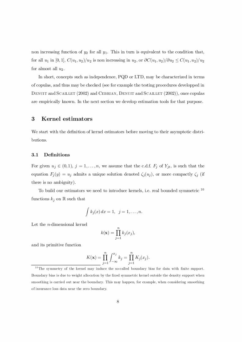
In short, concepts such as independence, PQD or LTD, may be characterized in terms
of copulas, and thus may be checked (see for example the testing procedures developped in
Denuit and Scaillet (2002) and Cebrian, Denuit and Scaillet (2002)), once copulas
are empirically known. In the next section we develop estimation tools for that purpose.
3 Kernel estimators
We start with the de…nition of kernel estimators before moving to their asymptotic distri-
butions.
3.1 De…nitions
For given uj 2 (0;1), j = 1; : : : ;n, we assume that the c.d.f. Fj of Yjt, is such that the
equation Fj(y) = uj admits a unique solution denoted ³j(uj), or more compactly ³j (if
there is no ambiguity).
To build our estimators we need to introduce kernels, i.e. real bounded symmetric 10
functions kj on R such that
Zkj(x)dx = 1; j = 1; : : : ;n:
Let the n-dimensional kernel
k(x) =nY
j=1kj(xj);
and its primitive function
K(x) =nY
j=1
Z xj¡1
kj =nY
j=1Kj(xj):
10 The symmetry of the kernel may induce the so-called boundary bias for data with …nite support.
Boundary bias is due to weight allocation by the …xed symmetric kernel outside the density support when
smoothing is carried out near the boundary. This may happen, for example, when considering smoothing
of insurance loss data near the zero boundary.
8
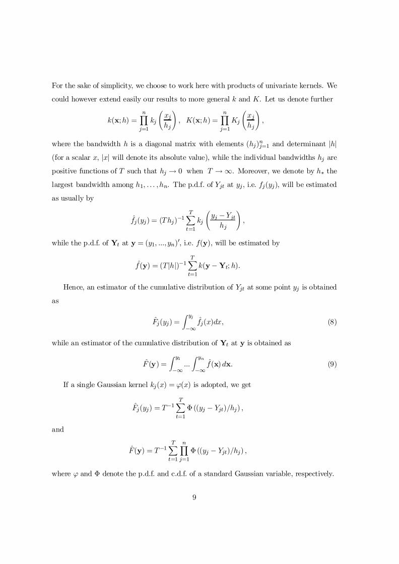
For the sake of simplicity, we choose to work here with products of univariate kernels. We
could however extend easily our results to more general k and K. Let us denote further
k(x;h) =nY
j=1kj
Ãxjhj
!; K(x;h) =
nY
j=1Kj
Ãxjhj
!;
where the bandwidth h is a diagonal matrix with elements (hj)nj=1 and determinant jhj(for a scalar x, jxj will denote its absolute value), while the individual bandwidths hj are
positive functions of T such that hj ! 0 when T ! 1. Moreover, we denote by h¤ the
largest bandwidth among h1; : : : ;hn. The p.d.f. of Yjt at yj , i.e. fj(yj), will be estimated
as usually by
fj(yj) = (Thj)¡1TX
t=1kj
Ãyj ¡Yjt
hj
!;
while the p.d.f. of Yt at y = (y1; :::; yn)0, i.e. f(y), will be estimated by
f(y) = (Tjhj)¡1TX
t=1k(y ¡ Yt; h):
Hence, an estimator of the cumulative distribution of Yjt at some point yj is obtained
as
Fj(yj) =Z yj¡1
fj(x)dx; (8)
while an estimator of the cumulative distribution of Yt at y is obtained as
F (y) =Z y1¡1
:::Z yn¡1
f(x)dx: (9)
If a single Gaussian kernel kj(x) = '(x) is adopted, we get
Fj(yj) = T¡1TX
t=1©((yj ¡ Yjt)=hj) ;
and
F(y) = T¡1TX
t=1
nY
j=1©((yj ¡ Yjt)=hj) ;
where ' and © denote the p.d.f. and c.d.f. of a standard Gaussian variable, respectively.
9
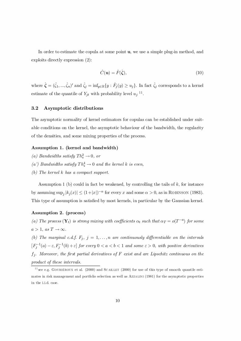
In order to estimate the copula at some point u, we use a simple plug-in method, and
exploits directly expression (2):
C(u) = F(³); (10)
where ³ = (³1; :::; ³n)0 and ³j = infy2Rfy : Fj(y) ¸ ujg. In fact ³j corresponds to a kernel
estimate of the quantile of Yjt with probability level uj 11.
3.2 Asymptotic distributions
The asymptotic normality of kernel estimators for copulas can be established under suit-
able conditions on the kernel, the asymptotic behaviour of the bandwidth, the regularity
of the densities, and some mixing properties of the process.
Assumption 1. (kernel and bandwidth)
(a) Bandwidths satisfy Th2¤ ! 0, or
(a’) Bandwidths satisfy Th4¤ ! 0 and the kernel k is even,
(b) The kernel k has a compact support.
Assumption 1 (b) could in fact be weakened, by controlling the tails of k, for instance
by assuming supj jkj(x)j · (1+jxj)¡® for every x and some ® > 0, as in Robinson (1983).
This type of assumption is satis…ed by most kernels, in particular by the Gaussian kernel.
Assumption 2. (process)
(a) The process (Yt) is strong mixing with coe¢cients ®t such that ®T = o(T¡a) for some
a > 1, as T ! 1.
(b) The marginal c.d.f. Fj, j = 1; : : : ;n are continuously di¤erentiable on the intervals
[F¡1j (a) ¡ "; F¡1
j (b)+ "] for every 0 < a < b < 1 and some " > 0, with positive derivatives
fj. Moreover, the …rst partial derivatives of F exist and are Lipschitz continuous on the
product of these intervals.11 see e.g. Gouriéroux et al. (2000) and Scaillet (2000) for use of this type of smooth quantile esti-
mates in risk management and portfolio selection as well as Azzalini (1981) for the asymptotic properties
in the i.i.d. case.
10
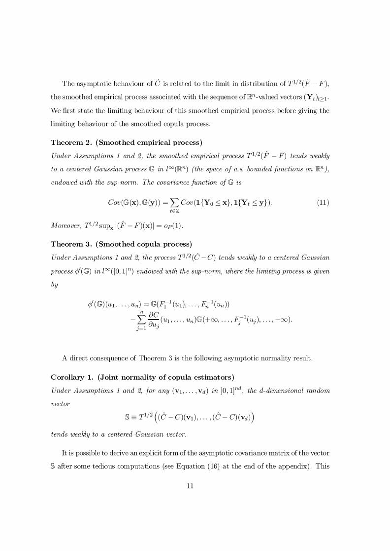
The asymptotic behaviour of C is related to the limit in distribution of T 1=2(F ¡F ),
the smoothed empirical process associated with the sequence of Rn-valued vectors (Yt)t¸1.
We …rst state the limiting behaviour of this smoothed empirical process before giving the
limiting behaviour of the smoothed copula process.
Theorem 2. (Smoothed empirical process)
Under Assumptions 1 and 2, the smoothed empirical process T 1=2(F ¡ F) tends weakly
to a centered Gaussian process G in l1(Rn) (the space of a.s. bounded functions on Rn),
endowed with the sup-norm. The covariance function of G is
Cov(G(x);G(y)) =X
t2ZCov(1fY0 · xg; 1fYt · yg): (11)
Moreover, T1=2 supx j(F ¡F )(x)j = oP(1).
Theorem 3. (Smoothed copula process)
Under Assumptions 1 and 2, the process T1=2(C ¡C) tends weakly to a centered Gaussian
process Á0(G) in l1([0;1]n) endowed with the sup-norm, where the limiting process is given
by
Á0(G)(u1; : : : ;un) = G(F¡11 (u1); : : : ; F¡1
n (un))
¡nX
j=1
@C@uj
(u1; : : : ; un)G(+1; : : : ; F¡1j (uj); : : : ; +1):
A direct consequence of Theorem 3 is the following asymptotic normality result.
Corollary 1. (Joint normality of copula estimators)
Under Assumptions 1 and 2, for any (v1; : : : ;vd) in ]0;1]nd, the d-dimensional random
vector
S ´ T1=2³(C ¡C)(v1); : : : ; (C ¡ C)(vd)
´
tends weakly to a centered Gaussian vector.
It is possible to derive an explicit form of the asymptotic covariance matrix of the vector
S after some tedious computations (see Equation (16) at the end of the appendix). This
11
covariance matrix will be used in the empirical section of this paper to build con…dence
intervals around copula estimates.
In the bivariate case Yt = (Y1t; Y2t)0, we have seen that positive quadrant depen-
dence is characterized by C(u1; u2) ¡ u1u2 ¸ 0, while left tail decreasing behaviour of
Y1t (resp. Y2t) in Y2t (resp. Y1t) is characterized by C(u1; u2)=u2 ¡ @C(u1;u2)=@u2 ¸ 0
(resp. C(u1;u2)=u1 ¡ @C(u1; u2)=@u1 ¸ 0). We have just developed a kernel estimator
for C . It is thus natural to suggest an estimator for @pC(u) = @C(u)=@up based on the
di¤erentiation of C(u) w.r.t. up:
\@pC(u) = @p³C(u)
´=
@pF(³)fp(³p)
;
with
³ = (³1; : : : ; ³n); ³j = F¡1j (uj); j = 1; : : : ; n;
and
@pF(³) =1
Thp
TX
t=1kp
óp¡ Ypt
hp
! Y
l 6=pKl
ól ¡ Ylt
hl
!:
The estimators C(u) and @pC(u) will help to detect positive quadrant dependence and
left tail decreasing behaviour through the empirical counterparts of the aforementioned
inequalities.
Assumption 3. (kernel and bandwidth)
(a) Bandwidths satisfy Thp ! +1, Th3¤ ! 0 and k is even,
(b) Each kernel kj has a compact support Aj, j = 1; : : : ; n, and the kernel kp is twice
continuously di¤erentiable.
Assumption 4. (process)
(a) The process (Yt) is strong mixing with coe¢cients ®t such that ®T = O(T¡2), as
T ! 1.
(b) The …rst derivative @pF and the marginal density fp are Lipschitz continuous.
(c) Let ft;t0 be the density function of (Yt; Yt0) with respect to the Lebesgue measure. There
exists an integrable function à : R2n¡2 ¡! R such that, for every vectors u; v in Rn, and
12
for some open subset O of R2 containing Ap £Ap, we have
supt6=t0
sup(up;vp)2O
ft;t0(u; v) · Ã(u¡p;v¡p):
Then we get:
Theorem 4. (Joint normality of derivative estimators)
Under Assumptions 3 and 4, for any u1; : : : ; ud 2]0;1[nd, the random vector
(Thp)1=2³(@pC ¡ @pC)(u1); : : : ; (@pC ¡@pC)(ud)
´
tends weakly to a centered Gaussian vector.
Again the asymptotic covariance matrix §¤ = [¾¤ij ]1·i;j·d of this random vector admits
a rather complex explicit form (see Equation (14) in the appendix).
Note that the extension of the previous propositions to higher derivatives
@kC(u)=(@u1@u2:::@uk), k · n, is straightforward. Such estimates are for example re-
quired for the implementation of an empirical counterpart of the simulation algorithm
described in Embrechts et al. (2002).
As clear from Theorem 4, a random vector of derivatives of T1=2(C ¡ C) at some
points u1; : : : ;ud does not in general tend weakly to a vector of independent Gaussian
variables. This is however the case when the components corresponding to the indices
of the derivatives are all di¤erent. A similar result is also true for successive derivatives.
Indeed, under some technical assumptions, the random vector
(Thm11 : : : : :hmnn )1=2
³@m11 : : : @mnn (C ¡ C)(u1); : : : ; @m1
1 : : : @mnn (C ¡C)(ud)´
tends weakly to a centered Gaussian vector whose covariance matrix is diagonal if
1. ml ¸ 1 for every l = 1; : : : ; n, or
2. for the indices l such that ml 6= 0, uli 6= ulj for every pair (i; j).
We end up this section with the description of how to build the sample analogues of
the dependence measures (3)-(6). First we may substitute a kernel estimator C for the
13
unknown C in (4)-(6) to estimate ½Y1 ;Y2 , °Y1;Y2, and ¯Y1;Y2. According to Theorem 3, these
estimators are consistent and asymptotically normally distributed. Second we may replace
the unkown derivatives by @C(u1;u2)=@u1 and @C(u1;u2)=@u2 in order to estimate ¿Y1;Y2.
This estimator will be consistent by Theorem 4.
4 Monte Carlo experiments
In this section we wish to investigate the …nite sample properties of our kernel estimators.
The experiments are based on a stationary vector autoregressive process of order one:
Yt = A + BYt¡1 + ºt;
where ºt » N(0;§) and all the eigenvalues of B are less than one in absolute value. The
marginal distribution of the process Y is Gaussian with mean ¹ = (Id ¡ B)¡1A and
covariance matrix satisfying vec = (Id ¡ B B)¡1vec§ (vecM is the stack of the
columns of the matrix M).
We start with a bivariate example where the components Y1t and Y2t are independent,
and thus C(u1;u2) = u1u2. The parameters are A = (1;1)0, vecB = (0:25;0;0; 0:75)0 and
vec§ = (:75; 0;0;1:25)0. The parameters of the Gaussian stationary distribution are then
¹ = (1:33; 4)0 and vec = (0:8; 0; 0;2:86)0. The number of Monte Carlo replications is
5,000, while the data length is T = 45 = 1024 (roughly four trading years of quotes).
The nonparametric estimators make use of the product of two Gaussian kernels. Band-
width values are based on the rule of thumb hi = ¾iT¡1=5, which uses the empirical
standard deviation of each series. Table 1 gives bias and mean squared error (MSE) 12
of the kernel estimates C(u1;u2) for several pairs (u1;u2) in the tails and center of the
distribution.
12 Recall that the bias is de…ned as EC ¡C and the MSE as E[(C ¡ C)2 ].
14
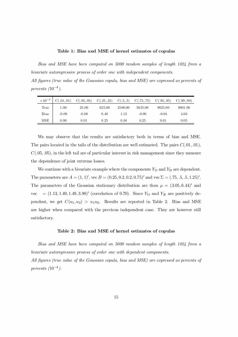
Table 1: Bias and MSE of kernel estimates of copulas
Bias and MSE have been computed on 5000 random samples of length 1024 from a
bivariate autoregressive process of order one with independent components.
All …gures (true value of the Gaussian copula, bias and MSE) are expressed as percents of
percents (10¡4).
£10¡4 C(.01,.01) C(.05,.05) C(.25,.25) C(.5,.5) C(.75,.75) C(.95,.95) C(.99,.99)
True 1.00 25.00 625.00 2500.00 5625.00 9025.00 9801.00
Bias -0.09 -0.08 0.40 1.12 -0.90 -0.04 4.66
MSE 0.00 0.01 0.25 0.48 0.25 0.01 0.05
We may observe that the results are satisfactory both in terms of bias and MSE.
The pairs located in the tails of the distribution are well estimated. The pairs C(:01; :01);
C(:05; :05); in the left tail are of particular interest in risk management since they measure
the dependence of joint extreme losses.
We continue with a bivariate examplewhere the components Y1t and Y2t are dependent.
The parameters are A = (1; 1)0, vecB = (0:25;0:2;0:2;0:75)0 and vec§ = (:75; :5; :5;1:25)0.
The parameters of the Gaussian stationary distribution are then ¹ = (3:05;6:44)0 and
vec = (1:13; 1:49; 1:49;3:98)0 (correlation of 0.70). Since Y1t and Y2t are positively de-
pendent, we get C(u1;u2) > u1u2. Results are reported in Table 2. Bias and MSE
are higher when compared with the previous independent case. They are however still
satisfactory.
Table 2: Bias and MSE of kernel estimates of copulas
Bias and MSE have been computed on 5000 random samples of length 1024 from a
bivariate autoregressive process of order one with dependent components.
All …gures (true value of the Gaussian copula, bias and MSE) are expressed as percents of
percents (10¡4).
15
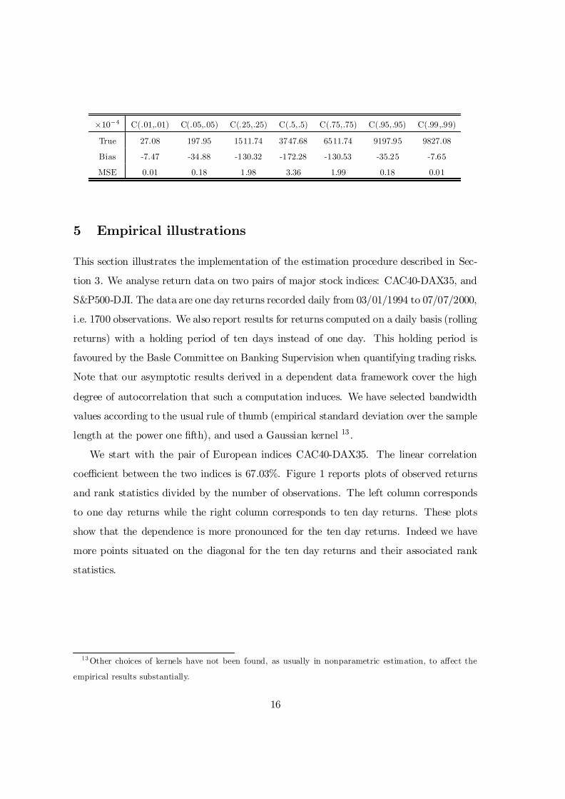
£10¡4 C(.01,.01) C(.05,.05) C(.25,.25) C(.5,.5) C(.75,.75) C(.95,.95) C(.99,.99)
True 27.08 197.95 1511.74 3747.68 6511.74 9197.95 9827.08
Bias -7.47 -34.88 -130.32 -172.28 -130.53 -35.25 -7.65
MSE 0.01 0.18 1.98 3.36 1.99 0.18 0.01
5 Empirical illustrations
This section illustrates the implementation of the estimation procedure described in Sec-
tion 3. We analyse return data on two pairs of major stock indices: CAC40-DAX35, and
S&P500-DJI. The data are one day returns recorded daily from 03/01/1994 to 07/07/2000,
i.e. 1700 observations. We also report results for returns computed on a daily basis (rolling
returns) with a holding period of ten days instead of one day. This holding period is
favoured by the Basle Committee on Banking Supervision when quantifying trading risks.
Note that our asymptotic results derived in a dependent data framework cover the high
degree of autocorrelation that such a computation induces. We have selected bandwidth
values according to the usual rule of thumb (empirical standard deviation over the sample
length at the power one …fth), and used a Gaussian kernel 13 .
We start with the pair of European indices CAC40-DAX35. The linear correlation
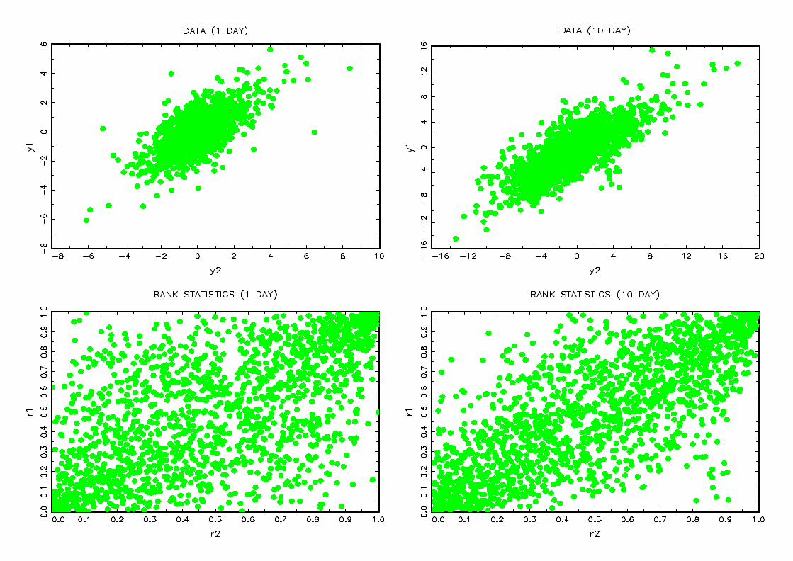
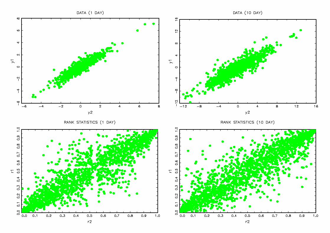
coe¢cient between the two indices is 67.03%. Figure 1 reports plots of observed returns
and rank statistics divided by the number of observations. The left column corresponds
to one day returns while the right column corresponds to ten day returns. These plots
show that the dependence is more pronounced for the ten day returns. Indeed we have
more points situated on the diagonal for the ten day returns and their associated rank
statistics.
13 Other choices of kernels have not been found, as usually in nonparametric estimation, to a¤ect the
empirical results substantially.
16
– Please insert Figure 1 –
Figure 1 : Returns and rank statistics for CAC40-DAX35
One day and ten day returns of the pair CAC40-DAX35 between 03/01/1994 and
07/07/2000 are plotted on the …rst line. The second line shows the associated rank statis-
tics divided by the number of observations.
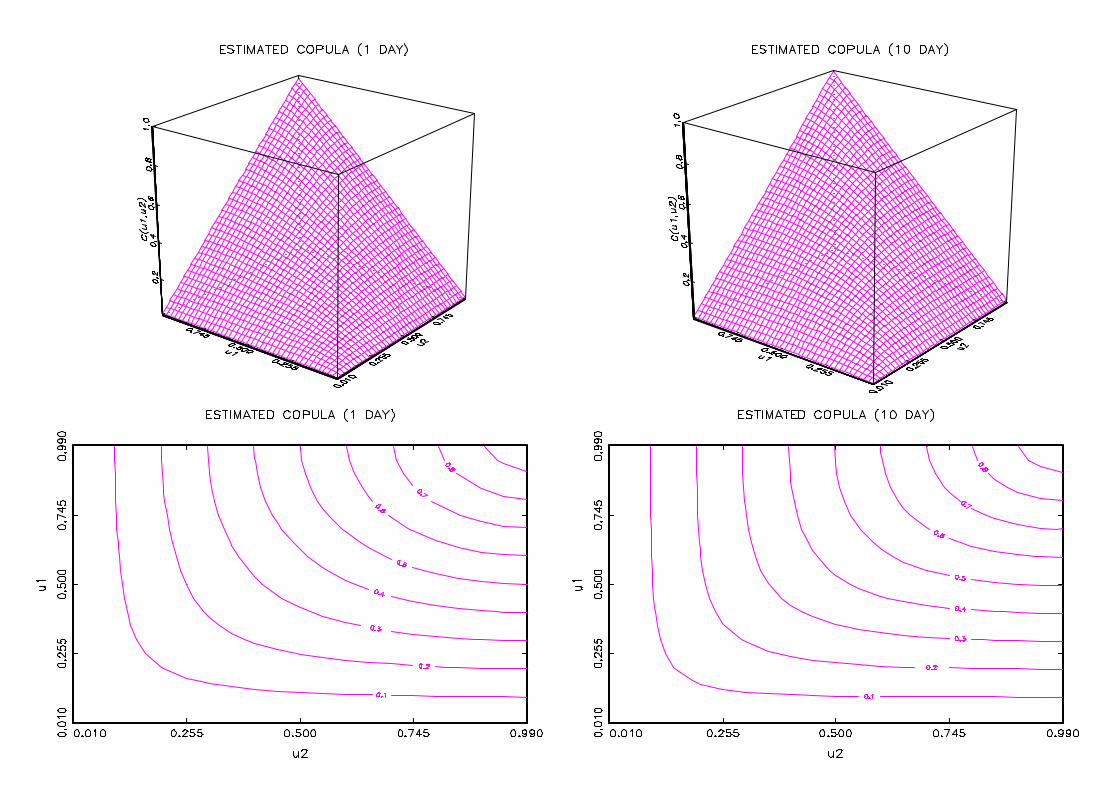
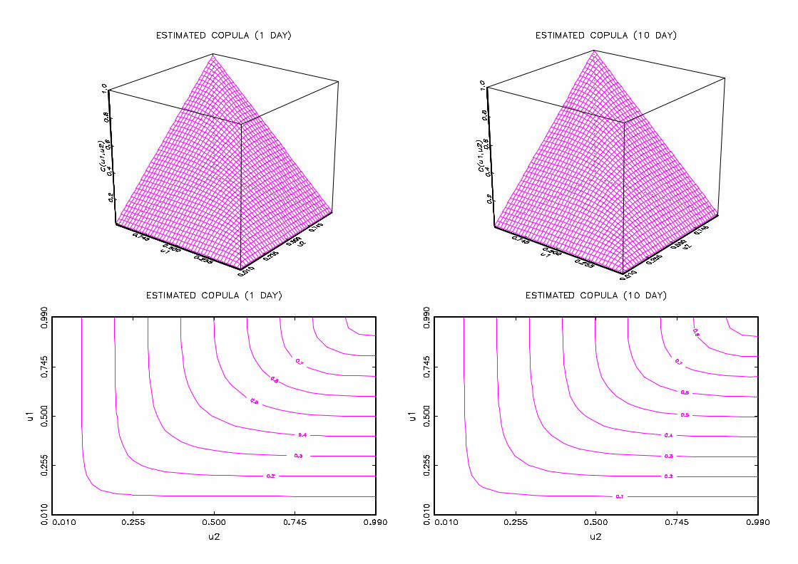
Figure 2 gives 3D and contour plots of estimated copulas. The contour plot for the
ten day returns is closer to the shape given by the comonotonic copula, namely successive
straight lines at right angles on the diagonal, which also indicates higher dependence for
the ten day returns.
– Please insert Figure 2 –
Figure 2 : Copula estimates and contour plots for CAC40-DAX35
Estimated copulas of one day and ten day returns of the pair CAC40-DAX35 between
03/01/1994 and 07/07/2000 are plotted on the …rst line. The second line shows the asso-
ciated contour plots.
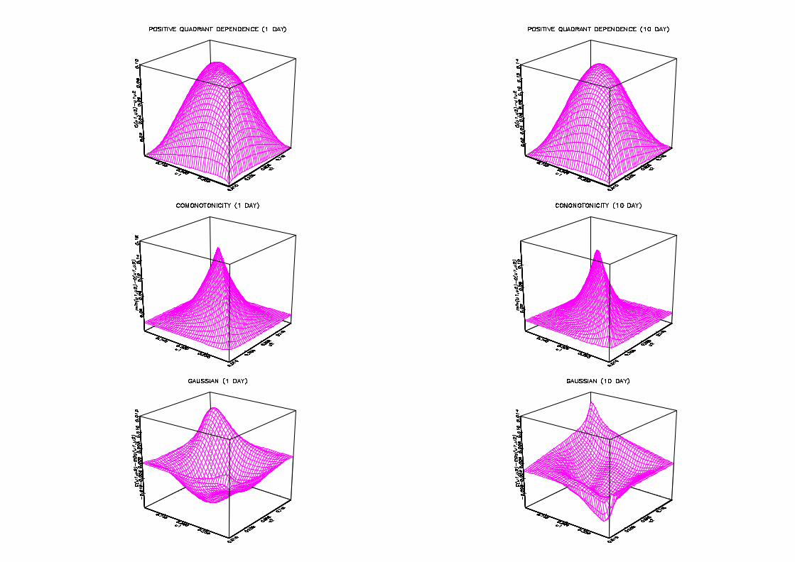
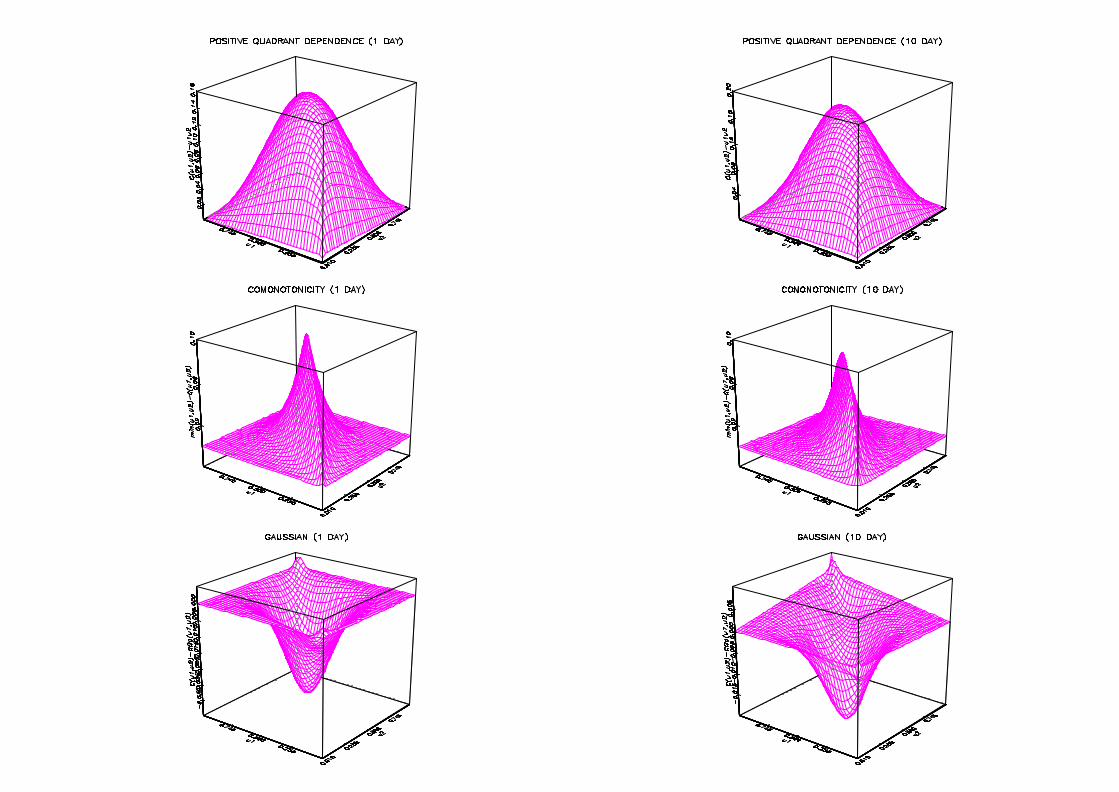
In Figure 3 we use estimates of the copulas to analyse positive quadrant dependence
(PQD). The …rst line of graphs shows that C(u1;u2) ¡ u1u2 is greater than zero, which
means that one day and ten day returns exhibit PQD. The di¤erence is larger in the
center of the distribution and decreases when we move to the extremes. Just below we …nd
comparison w.r.t. the comonotonic copula, i.e. min(u1; u2) ¡ C(u1;u2), and the Gaussian
copula, i.e. C(u1;u2) ¡ CGau(u1; u2; ½¤). The estimate ½¤ of the parameter ½¤ of the
Gaussian copula is obtained using the equation ½¤ = 2 sin(¼½=6) linking ½¤ with the rank
correlation ½ 14 . The hat of the ten day returns is lower than the hat of the one day14 Estimates obtained from the empirical rank correlation or its smoothed counterpart lead to virtually
identical results.
17
returns for comotonicity. This again indicates a higher dependence for the former than
for the latter. Interestingly the last line illustrates how smoothed copula estimates can be
used as graphical device to detect adequacy of parametric copula models. Indeed we may
observe that the Gaussian copula exhibits too low levels for small u1, u2 and large u1, u2.
In the center of the distribution this is the reverse.
– Please insert Figure 3 –
Figure 3 : Comparison with independent, comonotonic and Gaussian copulas
for CAC40-DAX35
The graphs successively compare nonparametric copula estimates with the independent
copula, the comonotonic copula and the Gaussian copula for the one day and ten day re-
turns of the pair CAC40-DAX35 between 03/01/1994 and 07/07/2000.
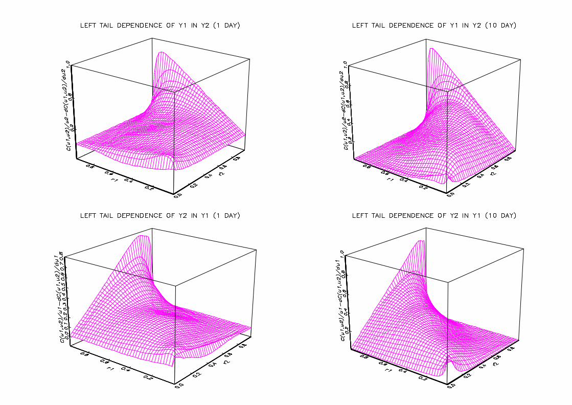
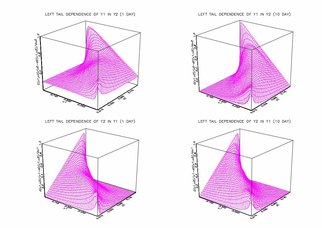
In Figure 4 copula derivatives are computed to study left tail decreasing behaviour
(LTD). The two lines carry graphs of C(u1;u2)=u2 ¡@C(u1;u2)=@u2, and C(u1; u2)=u1 ¡@C(u1;u2)=@u1, respectively. Again we get positiveness, and LTD is thus present for both
stock indices and both holding periods. Besides, LTD is heavier for the ten day holding
period.
– Please insert Figure 4 –
Figure 4 : Left tail decreasing behaviour for CAC40-DAX35
The graphs show the left tail decreasing behaviour of the one day and ten day returns
of the pair CAC40-DAX35 between 03/01/1994 and 07/07/2000.
For the pair of US indices S&P500-DJI, we get Figures 5-8. The linear correlation
coe¢cient is equal to 93.25%. Comments made for European indices carry over. However
the dependence is higher for US indices. Indeed we get further clustering around the
18
diagonal in Figure 5, even closer contour plots to the comonotonic plot in Figure 6, and
higher hats for positive quadrant dependence and comonotonicity in Figure 7.
– Please insert Figure 5 –
Figure 5 : Returns and rank statistics for S&P500-DJI
One day and ten day returns of the pair S&P500-DJI between 03/01/1994 and 07/07/2000
are plotted on the …rst line. The second line shows the associated order statistics divided
by the number of observations.
– Please insert Figure 6 –
Figure 6 : Copula estimates and contour plots for S&P500-DJI
Estimated copulas of one day and ten day returns of the pair S&P500-DJI between 03/01/1994
and 07/07/2000 are plotted on the …rst line. The second line shows the associated contour
plots.
– Please insert Figure 7 –
Figure 7 : Comparison with independent, comonotonic and Gaussian copulas
for S&P500-DJI
The graphs successively compare nonparametric copula estimates with the independent
copula, the comonotonic copula and the Gaussian copula for the one day and ten day
returns of the pair S&P500-DJI between 03/01/1994 and 07/07/2000.
19
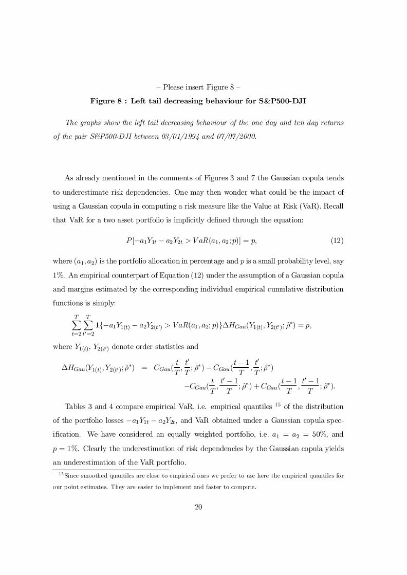
– Please insert Figure 8 –
Figure 8 : Left tail decreasing behaviour for S&P500-DJI
The graphs show the left tail decreasing behaviour of the one day and ten day returns
of the pair S&P500-DJI between 03/01/1994 and 07/07/2000.
As already mentioned in the comments of Figures 3 and 7 the Gaussian copula tends
to underestimate risk dependencies. One may then wonder what could be the impact of
using a Gaussian copula in computing a risk measure like the Value at Risk (VaR). Recall
that VaR for a two asset portfolio is implicitly de…ned through the equation:
P [¡a1Y1t ¡ a2Y2t > V aR(a1; a2;p)] = p; (12)
where (a1; a2) is the portfolio allocation in percentage and p is a small probability level, say
1%. An empirical counterpart of Equation (12) under the assumption of a Gaussian copula
and margins estimated by the corresponding individual empirical cumulative distribution
functions is simply:
TX
t=2
TX
t0=21f¡a1Y1(t) ¡ a2Y2(t0) > VaR(a1; a2; p)g¢HGau(Y1(t); Y2(t0); ½¤) = p;
where Y1(t), Y2(t0) denote order statistics and
¢HGau(Y1(t);Y2(t0); ½¤) = CGau(tT
;t0
T; ½¤) ¡CGau(
t ¡ 1T
;t0
T; ½¤)
¡CGau(tT
;t0 ¡ 1
T; ½¤) +CGau(
t ¡ 1T
;t0 ¡ 1
T; ½¤):
Tables 3 and 4 compare empirical VaR, i.e. empirical quantiles 15 of the distribution
of the portfolio losses ¡a1Y1t ¡ a2Y2t, and VaR obtained under a Gaussian copula spec-
i…cation. We have considered an equally weighted portfolio, i.e. a1 = a2 = 50%, and
p = 1%. Clearly the underestimation of risk dependencies by the Gaussian copula yields
an underestimation of the VaR portfolio.15 Since smoothed quantiles are close to empirical ones we prefer to use here the empirical quantiles for
our point estimates. They are easier to implement and faster to compute.
20
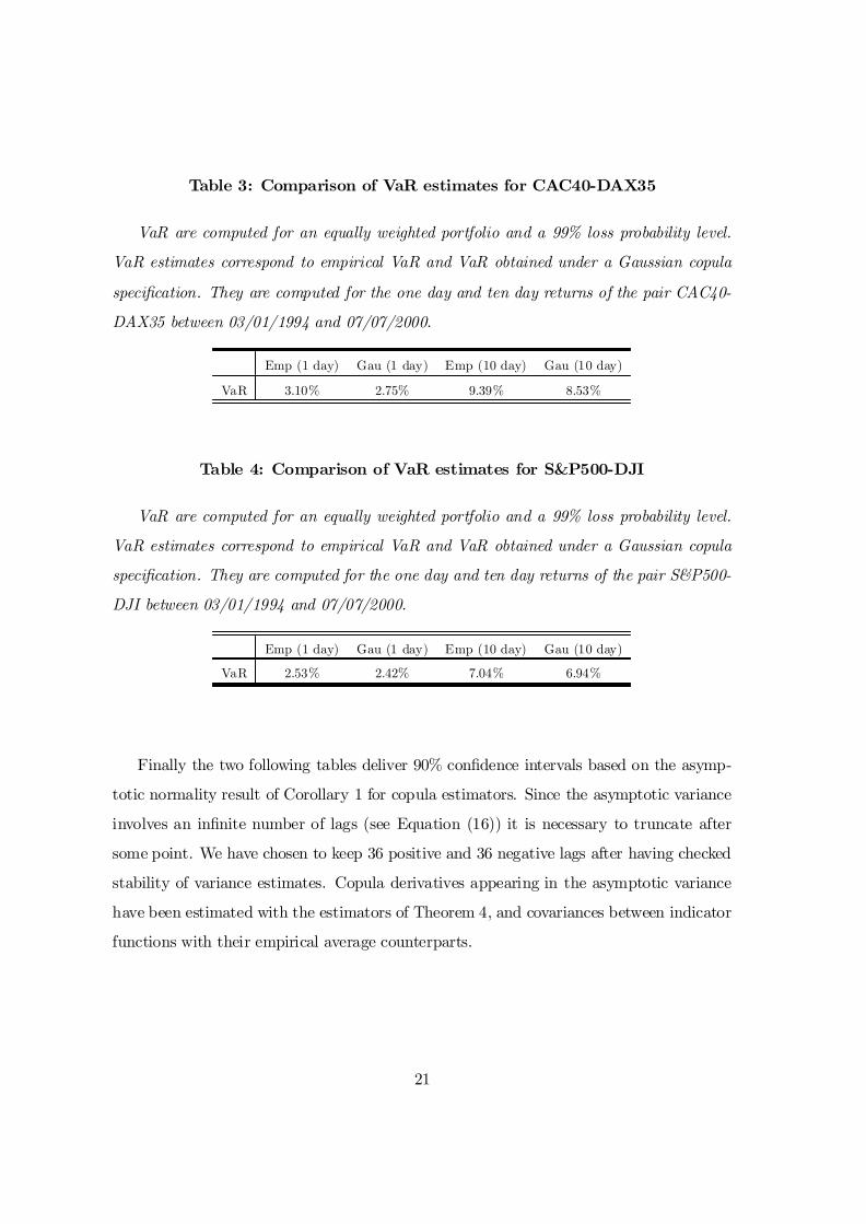
Table 3: Comparison of VaR estimates for CAC40-DAX35
VaR are computed for an equally weighted portfolio and a 99% loss probability level.
VaR estimates correspond to empirical VaR and VaR obtained under a Gaussian copula
speci…cation. They are computed for the one day and ten day returns of the pair CAC40-
DAX35 between 03/01/1994 and 07/07/2000.
Emp (1 day) Gau (1 day) Emp (10 day) Gau (10 day)
VaR 3.10% 2.75% 9.39% 8.53%
Table 4: Comparison of VaR estimates for S&P500-DJI
VaR are computed for an equally weighted portfolio and a 99% loss probability level.
VaR estimates correspond to empirical VaR and VaR obtained under a Gaussian copula
speci…cation. They are computed for the one day and ten day returns of the pair S&P500-
DJI between 03/01/1994 and 07/07/2000.
Emp (1 day) Gau (1 day) Emp (10 day) Gau (10 day)
VaR 2.53% 2.42% 7.04% 6.94%
Finally the two following tables deliver 90% con…dence intervals based on the asymp-
totic normality result of Corollary 1 for copula estimators. Since the asymptotic variance
involves an in…nite number of lags (see Equation (16)) it is necessary to truncate after
some point. We have chosen to keep 36 positive and 36 negative lags after having checked
stability of variance estimates. Copula derivatives appearing in the asymptotic variance
have been estimated with the estimators of Theorem 4, and covariances between indicator
functions with their empirical average counterparts.
21
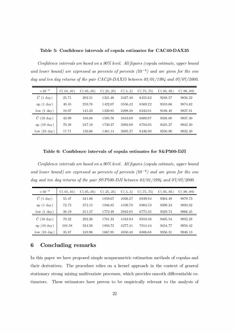
Table 5: Con…dence intervals of copula estimates for CAC40-DAX35
Con…dence intervals are based on a 90% level. All …gures (copula estimate, upper bound
and lower bound) are expressed as percents of percents (10¡4) and are given for the one
day and ten day returns of the pair CAC40-DAX35 between 03/01/1994 and 07/07/2000.
£10¡4 C(.01,.01) C(.05,.05) C(.25,.25) C(.5,.5) C(.75,.75) C(.95,.95) C(.99,.99)
C (1 day) 25.71 202.51 1321.46 3427.40 6455.62 9248.57 9856.22
up (1 day) 40.45 259.78 1422.07 3556.42 6569.22 9310.66 9874.62
low (1 day) 10.97 145.23 1220.85 3298.38 6342.01 9186.48 9837.81
C (10 day) 43.99 186.88 1595.76 3843.69 6609.97 9338.08 9937.30
up (10 day) 70.28 247.10 1730.37 3992.00 6783.05 9425.27 9942.20
low (10 day) 17.71 126.66 1461.14 3695.37 6436.90 9250.90 9932.40
Table 6: Con…dence intervals of copula estimates for S&P500-DJI
Con…dence intervals are based on a 90% level. All …gures (copula estimate, upper bound
and lower bound) are expressed as percents of percents (10¡4) and are given for the one
day and ten day returns of the pair S&P500-DJI between 03/01/1994 and 07/07/2000.
£10¡4 C(.01,.01) C(.05,.05) C(.25,.25) C(.5,.5) C(.75,.75) C(.95,.95) C(.99,.99)
C (1 day) 55.47 341.86 1859.67 4026.27 6839.94 9364.49 9879.73
up (1 day) 72.73 372.15 1946.85 4109.70 6904.53 9399.24 9893.02
low (1 day) 38.19 311.57 1772.49 3942.85 6775.35 9329.74 9866.45
C (10 day) 70.22 292.26 1781.33 4163.94 6910.56 9405.54 9952.28
up (10 day) 104.58 334.56 1894.72 4277.41 7014.44 9454.77 9958.42
low (10 day) 35.87 249.96 1667.95 4050.48 6806.68 9356.31 9946.13
6 Concluding remarks
In this paper we have proposed simple nonparametric estimation methods of copulas and
their derivatives. The procedure relies on a kernel approach in the context of general
stationary strong mixing multivariate processes, which provides smooth di¤erentiable es-
timators. These estimators have proven to be empirically relevant to the analysis of
22
dependencies among stock index returns. In particular they reveal the di¤erent types of
dependence structures present in these data. Hence they complement ideally the existing
battery of nonparametric tools by providing speci…c instruments dedicated to dependence
measurement and joint risk analysis. They should also help to design goodness-of-…t tests
for copulas. This is under current research.
23
APPENDIX
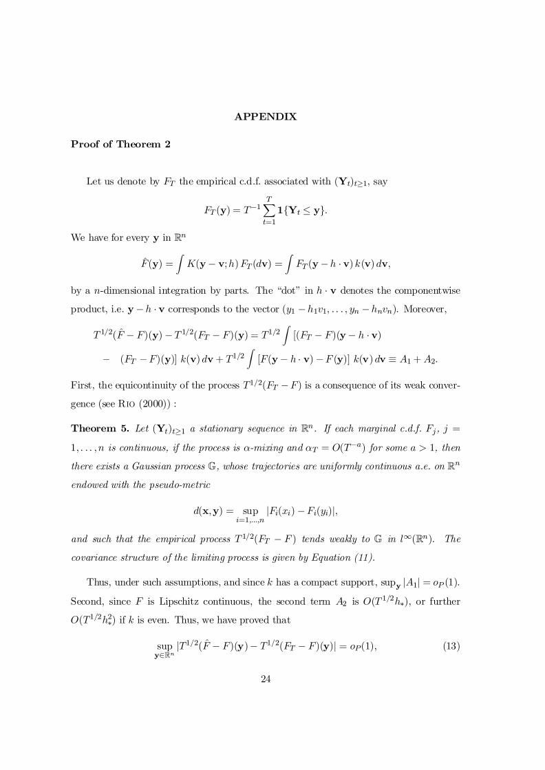
Proof of Theorem 2
Let us denote by FT the empirical c.d.f. associated with (Yt)t¸1, say
FT (y) = T¡1TX
t=11fYt · yg:
We have for every y in Rn
F(y) =Z
K(y ¡ v;h)FT (dv) =Z
FT (y ¡h ¢ v)k(v)dv;
by a n-dimensional integration by parts. The “dot” in h ¢ v denotes the componentwise
product, i.e. y ¡h ¢ v corresponds to the vector (y1 ¡h1v1; : : : ; yn ¡hnvn). Moreover,
T 1=2(F ¡ F)(y) ¡T 1=2(FT ¡ F)(y) = T1=2Z
[(FT ¡ F)(y ¡ h ¢ v)
¡ (FT ¡F)(y)] k(v)dv + T1=2Z
[F(y ¡ h ¢ v) ¡F (y)] k(v)dv ´ A1 + A2:
First, the equicontinuity of the process T1=2(FT ¡F) is a consequence of its weak conver-
gence (see Rio (2000)) :
Theorem 5. Let (Yt)t¸1 a stationary sequence in Rn. If each marginal c.d.f. Fj, j =
1; : : : ;n is continuous, if the process is ®-mixing and ®T = O(T¡a) for some a > 1, then
there exists a Gaussian process G, whose trajectories are uniformly continuous a.e. on Rn
endowed with the pseudo-metric
d(x;y) = supi=1;:::;n
jFi(xi) ¡Fi(yi)j;
and such that the empirical process T 1=2(FT ¡ F ) tends weakly to G in l1(Rn). The
covariance structure of the limiting process is given by Equation (11).
Thus, under such assumptions, and since k has a compact support, supy jA1j = oP (1).
Second, since F is Lipschitz continuous, the second term A2 is O(T 1=2h¤), or further
O(T1=2h2¤) if k is even. Thus, we have proved that
supy2Rn
jT1=2(F ¡ F)(y)¡ T1=2(FT ¡ F)(y)j = oP(1); (13)
24
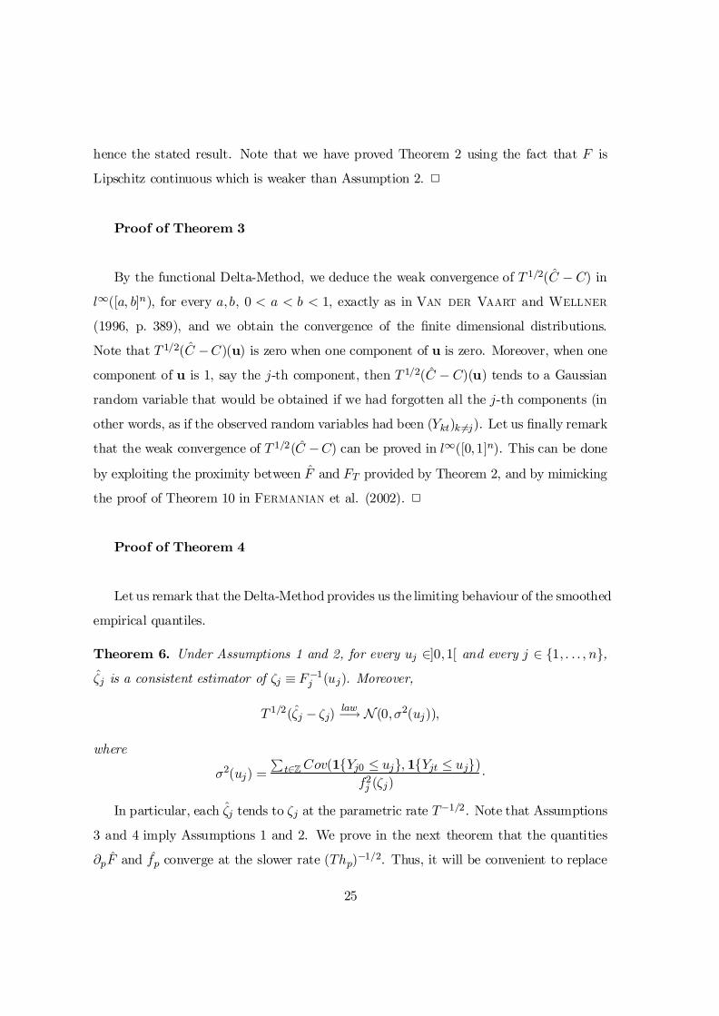
hence the stated result. Note that we have proved Theorem 2 using the fact that F is
Lipschitz continuous which is weaker than Assumption 2. 2
Proof of Theorem 3
By the functional Delta-Method, we deduce the weak convergence of T 1=2(C ¡ C) in
l1([a; b]n), for every a;b, 0 < a < b < 1, exactly as in Van der Vaart and Wellner
(1996, p. 389), and we obtain the convergence of the …nite dimensional distributions.
Note that T 1=2(C ¡C)(u) is zero when one component of u is zero. Moreover, when one
component of u is 1, say the j-th component, then T 1=2(C ¡ C)(u) tends to a Gaussian
random variable that would be obtained if we had forgotten all the j-th components (in
other words, as if the observed random variables had been (Ykt)k 6=j). Let us …nally remark
that the weak convergence of T 1=2(C ¡C) can be proved in l1([0;1]n). This can be done
by exploiting the proximity between F and FT provided by Theorem 2, and by mimicking
the proof of Theorem 10 in Fermanian et al. (2002). 2
Proof of Theorem 4
Letus remark that the Delta-Method provides us the limiting behaviour of the smoothed
empirical quantiles.
Theorem 6. Under Assumptions 1 and 2, for every uj 2]0;1[ and every j 2 f1; : : : ; ng,³j is a consistent estimator of ³j ´ F¡1
j (uj). Moreover,
T 1=2(³j ¡ ³j)law¡! N(0;¾2(uj));
where
¾2(uj) =Pt2Z Cov(1fYj0 · ujg; 1fYjt · ujg)
f2j (³j)¢
In particular, each ³j tends to ³j at the parametric rate T¡1=2. Note that Assumptions
3 and 4 imply Assumptions 1 and 2. We prove in the next theorem that the quantities
@pF and fp converge at the slower rate (Thp)¡1=2. Thus, it will be convenient to replace
25
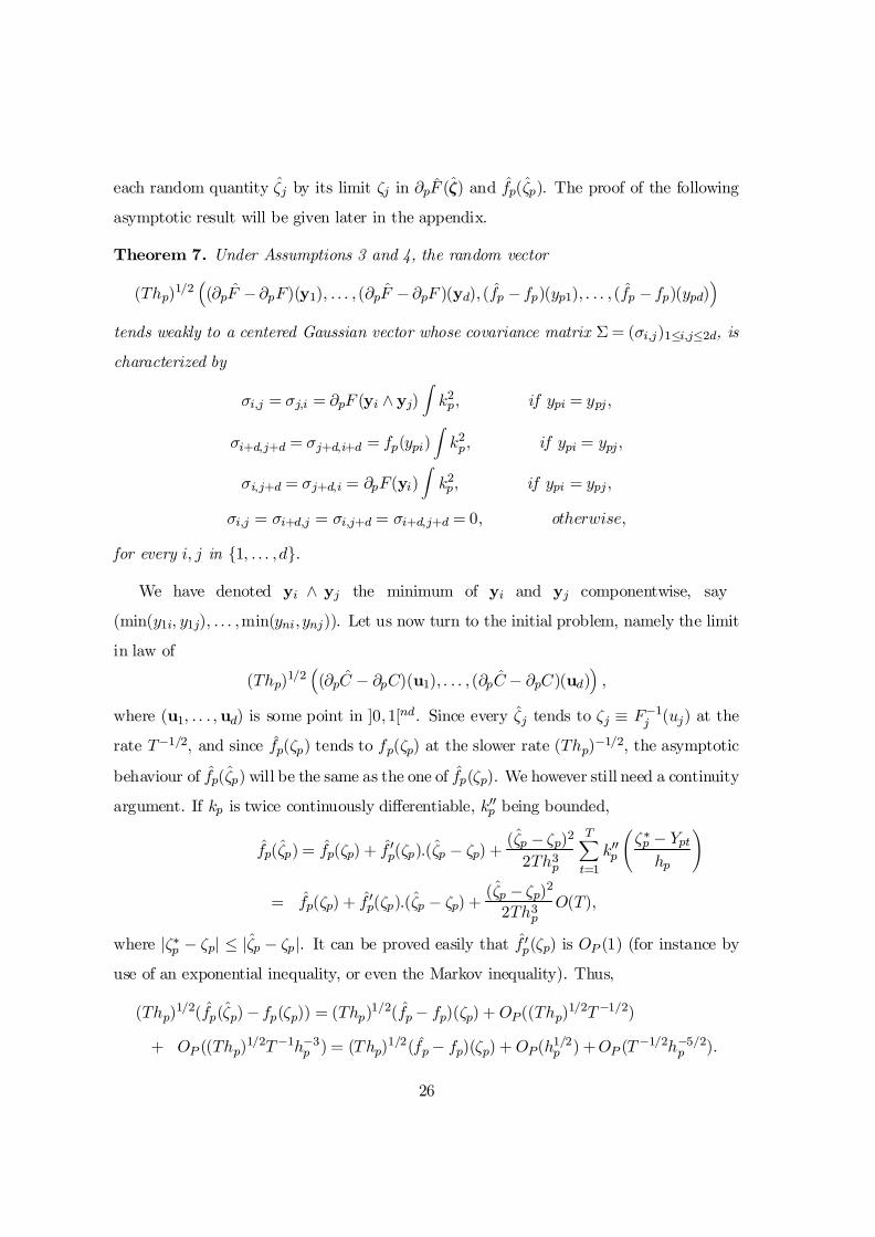
each random quantity ³j by its limit ³j in @pF (³) and fp(³p). The proof of the following
asymptotic result will be given later in the appendix.
Theorem 7. Under Assumptions 3 and 4, the random vector
(Thp)1=2³(@pF ¡@pF)(y1); : : : ; (@pF ¡@pF )(yd); (fp ¡ fp)(yp1); : : : ; (fp ¡ fp)(ypd)
´
tends weakly to a centered Gaussian vector whose covariance matrix § = (¾i;j)1·i;j·2d, is
characterized by
¾i;j = ¾j;i = @pF (yi ^ yj)Z
k2p; if ypi = ypj ;
¾i+d;j+d = ¾j+d;i+d = fp(ypi)Z
k2p; if ypi = ypj ;
¾i;j+d = ¾j+d;i = @pF(yi)Z
k2p; if ypi = ypj ;
¾i;j = ¾i+d;j = ¾i;j+d = ¾i+d;j+d = 0; otherwise;
for every i; j in f1; : : : ; dg.
We have denoted yi ^ yj the minimum of yi and yj componentwise, say
(min(y1i; y1j); : : : ;min(yni; ynj)). Let us now turn to the initial problem, namely the limit
in law of
(Thp)1=2³(@pC ¡ @pC)(u1); : : : ; (@pC ¡ @pC)(ud)
´;
where (u1; : : : ; ud) is some point in ]0;1[nd. Since every ³j tends to ³j ´ F¡1j (uj) at the
rate T¡1=2, and since fp(³p) tends to fp(³p) at the slower rate (Thp)¡1=2, the asymptotic
behaviour of fp(³p) will be the same as the one of fp(³p). We however still need a continuity
argument. If kp is twice continuously di¤erentiable, k00p being bounded,
fp(³p) = fp(³p) + f 0p(³p):(³p ¡ ³p) +(³p ¡ ³p)2
2Th3p
TX
t=1k00p
ó¤p ¡ Ypt
hp
!
= fp(³p) + f 0p(³p):(³p ¡ ³p) +(³p ¡ ³p)2
2Th3p
O(T);
where j³¤p ¡ ³pj · j³p ¡ ³pj. It can be proved easily that f 0p(³p) is OP (1) (for instance by
use of an exponential inequality, or even the Markov inequality). Thus,
(Thp)1=2(fp(³p) ¡ fp(³p)) = (Thp)1=2(fp¡ fp)(³p) + OP((Thp)1=2T¡1=2)
+ OP ((Thp)1=2T¡1h¡3p ) = (Thp)1=2(fp¡ fp)(³p) + OP(h1=2p ) +OP (T¡1=2h¡5=2p ):
26
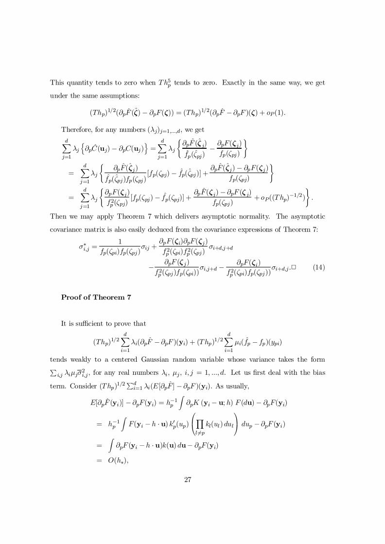
This quantity tends to zero when Th5p tends to zero. Exactly in the same way, we get
under the same assumptions:
(Thp)1=2(@pF (³) ¡ @pF(³)) = (Thp)1=2(@pF ¡@pF )(³) + oP(1):
Therefore, for any numbers (¸j)j=1;:::;d, we getdX
j=1jn@pC(uj) ¡ @pC(uj)
o=dX
j=1¸j
(@pF (³j)fp(³pj)
¡ @pF(³j)fp(³pj)
)
=dX
j=1¸j
(@pF(³j)
fp(³pj)fp(³pj)[fp(³pj) ¡ fp(³pj)] +
@pF(³j) ¡ @pF(³j)fp(³pj)
)
=dX
j=1¸j
(@pF(³j)f2p (³pj)
[fp(³pj) ¡ fp(³pj)] +@pF(³j) ¡@pF (³j)
fp(³pj)+ oP((Thp)¡1=2)
):
Then we may apply Theorem 7 which delivers asymptotic normality. The asymptotic
covariance matrix is also easily deduced from the covariance expressions of Theorem 7:
¾¤i;j =1
fp(³pi)fp(³pj)¾ij +
@pF(³i)@pF(³j)f2p (³pi)f2
p (³pj)¾i+d;j+d
¡ @pF (³j)f2p (³pj)fp(³pi))
¾i;j+d ¡ @pF(³i)f2p (³pi)fp(³pj))
¾i+d;j :2 (14)
Proof of Theorem 7
It is su¢cient to prove that
(Thp)1=2dX
i=1¸i(@pF ¡@pF )(yi) + (Thp)1=2
dX
i=1¹i(fp ¡ fp)(ypi)
tends weakly to a centered Gaussian random variable whose variance takes the formPi;j i¹j¾2
i;j , for any real numbers i, ¹j , i; j = 1; :::; d. Let us …rst deal with the bias
term. Consider (Thp)1=2Pdi=1 i(E[@pF ] ¡@pF )(yi). As usually,
E[@pF (yi)] ¡@pF(yi) = h¡1pZ
@pK (yi¡ u; h) F (du) ¡ @pF(yi)
= h¡1pZ
F(yi ¡h ¢ u)k0p(up)
0@Y
l 6=pkl(ul)dul
1A dup ¡@pF (yi)
=Z
@pF (yi ¡h ¢ u)k(u)du¡ @pF(yi)
= O(h¤);
27
since @pF is Lipschitz continuous. Then, this bias term is negligible under our assumptions.
Similarly, (Thp)1=2Pdi=1 ¹i(E[fp] ¡ f)(ypi) is o(1) under the same assumptions.
Second, to obtain the asymptotic normality, the simplest way to proceed is to apply
Lemma 7.1 in Robinson (1983) 16. In his notations, set p = 2d, ai = hp, as well as
VitT = ¸i f(@pK) (yi¡ Yt; h) ¡ E [(@pK) (yi ¡ Yt;h)]g ;
and
V ¤itT = ¹i fkp (ypi ¡Ypt; hp) ¡ E [kp (ypi¡ Ypt;hp)]g :
We now verify the conditions of validity of Lemma 7.1 in Robinson (1983).
Note that, by successive integration by parts, we get
E[V 2itT] = ¸2i
(Z(@pK)2 (yi ¡u;h) F(du) ¡
µZ(@pK) (yi ¡u;h) F(du)
¶2)
= ¸2i
8><>:
ZF(yi ¡h ¢ u)2n(kk0)p(up)
Y
l6=p(kK)l(ul)du ¡
0@
ZF(yi¡ h ¢ u)k0p(up)
Y
l 6=pkl(ul)du
1A
29>=>;
= hp¸2i
8<:
Z@pF(yi¡ h ¢ u)2n¡1k2p(up)
Y
l6=p(kK)l(ul)du
¡ hp
0@
Z@pF(yi ¡ h ¢ u)kp(up)
Y
l6=pkl(ul)du
1A
29>=>;
= 2n¡1hp¸2i@pF (yi)
Zk2p(up)
Y
l 6=p(kK)l(ul)du+ O(h2¤) = ¸2ihp¾
2ii + O(h2¤):
Moreover, by similar computations, if i 6= j,
E[VitTVjtT ] = ¸i¸j½Z
(@pK) (yi ¡u;h) (@pK) (yj ¡ u; h) F (du)
¡µZ
(@pK) (yi¡ u; h) F(du)¶
:µZ
(@pK) (yj ¡u;h) F(du)¶¾
= ¸i¸j½Z
F(yi¡ h ¢ u)hk0p(up)kp((ypj ¡ ypi)=hp+ up) + kp(up)k0p((ypj ¡ ypi)=hp +up)
i
¢Y
l6=p[kl(ul)Kl((ylj ¡ yli)=hl +ul) +Kl(ul)kl((ylj ¡ yli)=hl +ul)] du+ O(h2¤):
9=;
16 see e.g. Bierens (1985) or Bosq (1998) for some alternative sets of assumptions
28
If yip 6= yjp, then kp((ypi¡ypj)=hp+up) and k0p((ypi¡ypj)=hp+up) is zero for every up 2 Ap,
for hp su¢ciently small. We get that E[VitTVjtT ] = 0 in this case, for T su¢ciently large.
Thus, let us assume ypi = ypj . For any index l 6= p, notice that Kl((ylj ¡ yli)=hl + ul)
is zero if ylj < yli and is one if ylj > yli, for T su¢ciently large. In the …rst case,
set the change of variable yli ¡ hl:ul = ylj ¡ hl:vl. The l-th factor in brackets becomes
kl(vl)Kl((yli¡ ylj)=hl + vl), which is kl(vl) for T su¢ciently large. In the second case, the
latter factor is kl(ul). Thus, E[VitTVjtT]) is nonzero only if ypi = ypj and, for T su¢ciently
large,
E[VitTVjtT ] = ¸i¸j
8<:
ZF(yi ^ yj ¡ h ¢ u)2k0p(up)kp(up) ¢
Y
l 6=pkl(ul)du +O(h2
¤):
9=; (15)
By an integration by parts with respect to up (similarly as for E[V 2itT ]), we get easily
E[VitTVjtT] = i jhp¾2ij + o(h¤):
Similar computations yield
E[V ¤itTV ¤
jtT ] = hp¹i¹jfp(ypi)Z
k2p + oP(hp);
if ypi = ypi, and E[V ¤itTV
¤jtT] = oP(hp) otherwise. Moreover,
E[V ¤itTVjtT ] = ¹i¸j
Zkp
Ãypi ¡up
hp
!(@pK) (yj ¡ u; h) F(du)+ OP(h2
p)
= ¹i jZ
F(yj ¡h ¢ u)Y
l6=pkl(ul)
(kp(up)k0p
Ãypi ¡ ypj
hp+up
!
+ k0p(up)kp
Ãypi ¡ ypj
hp+up
!)du +OP(h2p):
If ypi 6= ypj , the latter quantity is zero for T su¢ciently large. Otherwise, it is equivalent
to ¹i jhp@pF(yj)R
k2p.
29
Thus, condition A:7:3 of Robinson (1983) is satis…ed. It remains to verify condition
A:7:4. For every i 6= j and t 6= t0,
E[jVitTVjt0Tj] = i j
Z ¯¯(@pK) (yi ¡ u;h) ¡
µZ(@pK) (yi ¡u;h) F(du)
¶¯¯
¢¯¯(@pK) (yj ¡ v; h) ¡
µZ(@pK) (yj ¡ v;h) F(dv)
¶¯¯ F(Yt;Yt0)(du; dv)
· Cst:h2p i jZ 0
@¯¯¯kp(up)
Y
l 6=pKl
µyli¡ ul
h
¶¯¯¯ + 1
1A
0@
¯¯¯kp(vp)
Y
l 6=pKl
µylj ¡ vl
h
¶¯¯¯ +1
1A
ft;t0(u¡p; ypi ¡ hpup;v¡p; ypj ¡hpvp)du dv:
Under our assumptions, the latter quantity if O(h2¤). Using similar boundings the same
property is satis…ed for E[jVitTV ¤jt0T j] and E[jV ¤
itTV ¤jt0T j].
The other conditions of Lemma 7.1 in Robinson (1983) are clearly satis…ed. Note
that our condition 4 (a) implies Robinson’s one on the mixing coe¢cients, i.e.P+1t=T ®t =
O(T¡1). Hence we have indeed proved the stated result. 2
30
Asymptotic covariance matrix in Corollary 1
The limiting distribution of S is a centered Gaussian vector whose covariance matrix
has the following (i; j)-th term:
E[Á0(G)(vi)Á0(G)(vj)] = E[G(³i)G(³j)] ¡nX
k=1@kC(vi)E[G(+1; : : : ; ³ki; : : : ; +1)G(³j)]
¡nX
k=1@kC(vj)E[G(+1; : : : ; ³kj ; : : : ; +1)G(³i)]
+nX
k;l=1@kC(vi)@lC(vj)E[G(+1; : : : ; ³ki; : : : ; +1)G(+1; : : : ; ³lj ; : : : ; +1)]
As previously, for every i = 1; : : : ; d, we have denoted by ³i the n-dimensional vector
(³1i; : : : ; ³ni) = (F¡11 (v1i); : : : ;F¡1
n (vni)):
Recalling Equation (11), we get
E[Á0(G)(vi)Á0(G)(vj)] =X
t2ZCov(1fY0 · ³ig;1fYt · ³jg)
¡nX
k=1@kC(vi)
X
t2ZCov(1fY0k · ³kig;1fYt · ³jg)
¡nX
k=1@kC(vj)
X
t2ZCov(1fY0 · ³ig;1fYtk · ³kjg)
+nX
k;l=1@kC(vi)@lC(vj)
X
t2ZCov(1fY0k · ³kig;1fYtl · ³ljg): (16)
References
[1] Azzalini, A. (1981). A Note on the Estimation of a Distribution Function and
Quantiles by a Kernel Method. Biometrika, 68, 326-328.
[2] Bierens, H. (1985). Kernel Estimators of Regression Functions. Advances in Econo-
metrics, Cambridge University Press, Cambridge, 99-144.
[3] Bosq, D. (1998). Nonparametric Statistics for Stochastic Processes: Estimation and
Prediction. Lecture Notes in Statistics, Springer-Verlag, New-York.
31
[4] Bouyé, E., V. Durrleman, A. Nikeghbali, G. Riboulet, and T. Roncalli
(2000). Copulas for …nance. A reading guide and some applications. GRO, Crédit
Lyonnais. Available on the web.
[5] Cebrian, A., M. Denuit, and O. Scaillet (2002). Testing for Concordance Or-
dering. DP FAME 41.
[6] Denuit, M., and O. Scaillet (2002). Nonparametric Tests for Positive Quadrant
Dependence. DP FAME 44.
[7] Deheuvels, P. (1979). La fonction de dépendance empirique et ses propriétés. Un
test non paramétrique d’indépendance. Acad. R. Belg., Bull. Cl. Sci., 5 Série, 65,
274-292.
[8] Deheuvels, P. (1981a). A Kolmogorov-Smirnov type test for independence and
multivariate samples. Rev. Roum. Math. Pures et Appl., Tome XXVI, 2, 213-226.
[9] Deheuvels, P. (1981b). A Nonparametric Test of Independence. Publications de
l’ISUP, 26, 29-50.
[10] Doukhan, P. (1994). Mixing: Properties and Examples. Lecture Notes in Statistics,
Springer-Verlag, New-York.
[11] Embrechts, P., A. McNeil, and D. Straumann (2002). Correlation and Depen-
dence in Risk Management: Properties and Pitfalls, in Risk Management: Value at
Risk and Beyond edited by Dempster M., Cambridge University Press, Cambridge.
[12] Fermanian, J.D., D. Radulovic, and M. Wegkamp (2002). Weak convergence
of empirical copula process. Working Paper CREST 2002 ¡ 06.
[13] Frees, E., and E. Valdez (1998). Understanding Relationships Using Copulas.
North American Actuarial J., 2, 1 ¡ 25.
[14] Frey, R., and A. McNeil (2001). Modelling dependent defaults. Working paper.
32
[15] Genest, C., Ghoudi, K. and L.P. Rivest (1993). A semiparametric estimation
procedure of dependence parameters in multivariate families of distributions. Bio-
metrika, 82, 543-552.
[16] Gouriéroux, C., J.P. Laurent and O. Scaillet (2000). Sensitivity Analysis of
Values at Risk. Journal of Empirical Finance, 7, 225-245.
[17] Joe, H. (1997). Multivariate Models and Dependence Concepts. Chapman & Hall,
London.
[18] Lehmann, E. (1966). Some Concepts of Dependence. Annals of Mathematical Sta-
tistics, 37, 1137-1153.
[19] Li, D. (2000). On default correlation : A copula function approach. Journal of Fixed
Income, 9, 43-54.
[20] Nelsen, R. (1999). An Introduction to Copulas. Lecture Notes in Statistics,
Springer-Verlag, New-York.
[21] Patton, A. (2001a). Modelling Time-Varying Exchange Rate Dependence Using the
Conditional Copula. UCSD WP 2001-09.
[22] Patton, A. (2001b). Estimation of Copula Models for Time Series of Possibly Dif-
ferent Lengths. UCSD WP 2001-17.
[23] Rio, E. (2000). Théorie Asymptotique des Processus Aléatoires Faiblement Dépen-
dants. SMAI, Springer.
[24] Robinson, P. (1983). Nonparametric Estimators for Time Series. Journal of Time
Series Analysis, 4, 185-207.
[25] Rockinger, M., and E. Jondeau (2001). Conditional Dependency of Financial
Series: An Application of Copulas. HEC Paris DP 723.
[26] Scaillet, O. (2000). Nonparametric Estimation and Sensitivity Analysis of Ex-
pected Shortfall, forthcoming in Mathematical Finance.
33
[27] Shi, J., and T. Louis (1995). Inferences on the association parameter in copula
models for bivariate survival data. Biometrics, 51, 1384-1399.
[28] Tjostheim, D. (1996). Measures of Dependence and Tests of Independence. Statis-
tics, 28, 249-284.
[29] Van der Vaart, A., and J. Wellner (1996). Weak Convergence and Empirical
Processes. Springer-Verlag, New York.
34
Figures 1-8
Figure 1 : Returns and rank statistics for CAC40-DAX35
Figure 2 : Copula estimates and contour plots for CAC40-DAX35
Figure 3 : Comparison with independent, comonotonic and Gaussian copu-
las for CAC40-DAX35
Figure 4 : Left tail decreasing behaviour for CAC40-DAX35
Figure 5 : Returns and rank statistics for S&P500-DJI
Figure 6 : Copula estimates and contour plots for S&P500-DJI
Figure 7 : Comparison with independent, comonotonic and Gaussian copu-
las for S&P500-DJI
Figure 8 : Left tail decreasing behaviour for S&P500-DJI
35