NONPARAMETRIC ESTIMATION OF THE INCUBATION TIMEDISTRIBUTION

BY PIET GROENEBOOM

Delft University of Technology

Delft University of Technology, Mekelweg 4, 2628 CD Delft, The Netherlands.P.Groeneboom@tudelft.nl

We discuss nonparametric estimators of the distribution of the incubationtime of a disease. The classical approach in these models is to use paramet-ric families like Weibull, log-normal or gamma in the estimation procedure.We analyze instead the nonparametric maximum likelihood estimator (MLE)and show that, under some conditions, its rate of convergence is cube root nand that its limit behavior is given by Chernoff’s distribution. We also studysmooth estimates, based on the MLE. The density estimates, based on theMLE, are capable of catching finer or unexpected aspects of the density, incontrast with the classical parametric methods. R scripts are provided for thenonparametric methods.

1. Introduction. In the original treatment of classical statistical inverse problems suchas the current status model it was assumed that the nonparametric maximum likelihood esti-mator (MLE) would converge as a process at

√n rate and in particular would be “tight”. It

was also conjectured that the pointwise limit distribution would be normal ([15], [17], [13]).But it was proved in [6] that the process is not tight, does not pointwise converge at

√n rate,

and that the actual pointwise limit distribution is also not normal, but in fact given by Cher-noff’s distribution (see [4] and [12]). This fact was for example noticed in [20], who refer forthe result to [11], where it is also given.

On the other hand, if we consider differentiable functionals of the model, we are backin√n asymptotics, with normal limit distributions. Theorem 3.1 on p. 183 of [19] gives

necessary and sufficient conditions for a functional to be differentiable in a very generalsetting. We give a short account of the (for us) relevant facts here, also summarized in [5] and[7].

We need the concept of Hellinger differentiability. Let the unknown distribution P on(Y,B) be contained in some class of probability measures P , which is dominated by a σ-finite measure µ. Let P have density p with respect to µ. We are interested in estimatingsome real-valued function Θ(P ) of P .

Let, for some δ > 0, the collection {Pt} with t ∈ (0, δ) be a 1-dimensional parametricsubmodel which is smooth in the following sense:∫ [

t−1(√pt −√p)− 1

2a√p

]2dµ→ 0 as t ↓ 0, for some a ∈ L2(P )

Such a submodel is called Hellinger differentiable. This property can be seen as an L2 versionof the pointwise differentiability of log pt(x) at t = 0 (with p0 = p), with the function aplaying the role of the so-called score-function ∂

∂t log pt(·)∣∣t=0

in classical statistics. For we

AMS 2000 subject classifications: Primary 62G05, 62N01; secondary 62-04.Keywords and phrases: nonparametric MLE, Chernoff’s distribution, kernel estimates, Weibull distribution,

incubation time, COVID-19.

1

2 P. GROENEBOOM

have,

limt↓0

√pt −√p0

t=

1

2√p0

∂

∂tpt

∣∣∣∣t=0

=1

2

(∂

∂tlog pt

∣∣∣∣t=0

)√p0 =

1

2a√p0

Therefore, a is also called the score function or score. The collection of scores a obtained byconsidering all possible one-dimensional Hellinger differentiable parametric submodels, is alinear space, the tangent space at P , denoted by T (P ).

In the models for inverse problems, to be considered in this paper, we work with a so-called hidden space and an observation space. All Hellinger differentiable submodels thatcan be formed in the observation space, together with the corresponding score functions, areinduced by the Hellinger differentiable paths of densities on the hidden space, according tothe following theorem:

THEOREM 1. Let P � µ be a class of probability measures on the hidden space (Y,B).P ∈ P is induced by the random vector Y . Suppose that the path {Pt} to P satisfies∫ [

t−1(√pt −√p)− 1

2a√p

]2dµ→ 0 as t ↓ 0

for some a ∈ L02(P ), where the superscript 0 means that

∫adP = 0.

Let S : (Y,B) → (Z,C) be a measurable mapping. Suppose that the induced measuresQt = PtS

−1 and Q = PS−1 on (Z,C) are absolutely continuous with respect to µS−1,with densities qt and q. Then the path {Qt} is also Hellinger differentiable, satisfying∫ [

t−1(√qt −√q)− 1

2a√q

]2dµS−1→ 0 as t ↓ 0

with a(z) =EP (a(Y )|S = z).

For a proof, see [2]. Note that a ∈ L02(Q). The relation between the scores a in the hidden

tangent space T (P ) and the induced scores a is expressed by the mapping

A : a(·) 7→EP (a(Y )|S = ·).(1.1)

This mapping is called the score operator. It is continuous and linear. Its range is the inducedtangent space, which is contained in L0

2(Q).Now Θ : P → R is pathwise differentiable at P if for each Hellinger differentiable path

{Pt}, with corresponding score a, we have

limt↓0

t−1(Θ(Pt)−Θ(P )) = Θ′P (a),

where

Θ′P : T (P )→R

is continuous and linear.Θ′P can be written in an inner product form. Since the tangent space T (P ) is a subspace

of the Hilbert-space L2(P ), the continuous linear functional Θ′P can be extended to a con-tinuous linear functional Θ

′P on L2(P ). By the Riesz representation theorem, to Θ

′P belongs

a unique θP ∈ L2(P ), called the gradient, satisfying

Θ′P (h) =< θP , h >P for all h ∈ L2(P ).

One gradient is playing a special role, which is obtained by extending T (P ) to the Hilbertspace T (P ). Then, the extension of Θ′P is unique, yielding the canonical gradient or efficient

INCUBATION TIME 3

influence function θP ∈ T (P ). This canonical gradient is also obtained by taking the orthog-onal projection of any gradient θP , obtained after extension of Θ′P , into T (P ). Hence θP isthe gradient with minimal norm among all gradients and we have (Pythagoras):

‖θP ‖2P = ‖θP ‖2P + ‖θP − θP ‖2P .

In our censoring model, differentiability of a functional Θ(Q) along the induced Hellingerdifferentiable paths in the observation space can be proved by looking at the structure of theadjoint A∗ of the score operator A according to theorem 2 below, which was first proved in[19] in a more general setting, allowing for Banach space valued functions as estimand. Thenthe proof is slightly more elaborate.

Recall that the adjoint of a continuous linear mapping A :G→H , with G and H Hilbert-spaces, is the unique continuous linear mapping A∗ :H→G satisfying

<Ag,h >H=< g,A∗h >G ∀g ∈G,h ∈H.

The score operator from (1.1) is playing the role of A. Its adjoint can be written as a condi-tional expectation as well. If Z ∼ PS−1, then:

[A∗ b](y) =EP (b(Z)|Y = y) a.e.-[P ]

THEOREM 2. Let Q=PS−1 be a class of probability measures on the image spaceof the measurable transformation S. Suppose the functional Θ : Q→ R can be written asΘ(Q) = K(P ) with K pathwise differentiable at P in the hidden space, having canonicalgradient κ.Then Θ is differentiable at QP ∈Q along the collection of induced paths in the observationspace obtained via Theorem 1 if and only if

(1.2) κ ∈R(A∗),

where A is the score operator. If (1.2) holds, then the canonical gradient θ of Θ and κ of Kare related by

κ=A∗θ.

We consider the following model, used for estimating the distribution of the incubationtime of a disease. In this model there is an infection time U , uniformly distributed on aninterval [0,E], where E (“exposure time”) has an absolutely continuous distribution functionFE on an interval [0,M2], and where U is uniform on [0,E], conditionally on E. Moreoverthere is an incubation time V with an absolutely continuous distribution F on an interval[0,M1] and a time for getting symptomatic S, where S = U + V . We assume that U and Vare independent, conditionally on E. Our observations consist of the pairs

(Ei, Si), i= 1, . . . , n.

The model is for example considered in [16], [3], [1] and [9].We define the (convolution) density qF by

qF (e, s) = e−1{F (s)− F (s− e)}= e−1∫ s

u=(s−e)+dF (u), e > 0, s ∈ [0,M1 +M2],

(1.3)

w.r.t. µ, which is the product of the measure dFE of the exposure time E and Lebesguemeasure on [0,M1 + M2], where M1 > 0 is the upper bound for the incubation time andM2 > 0 is the upper bound for the exposure time.

4 P. GROENEBOOM

For estimating the distribution function F0 of the incubation time, usually parametric dis-tributions are used, like the Weibull, log-normal or gamma distribution. However, in [9] thenonparametric maximum likelihood estimator is used. The maximum likelihood estimatorFn maximizes the function

`(F ) = n−1n∑

i=1

log {F (Si)− F (Si −Ei)}=

∫log{F (s)− F (s− e)}dQn(e, s)(1.4)

over all distribution functions F on R which satisfy F (x) = 0, x ≤ 0, see [9]. Here Qn isthe empirical distribution function of the pairs (Ei, Si), i= 1, . . . , n. We’ll prove that, undersome conditions on the underlying distributions, the MLE Fn of the incubation time hascube root n convergence and converges in distribution, after standardization, to Chernoff’sdistribution, see Theorem 4.

So this is a clear example of a situation where the MLE doe not converge pointwise at√n rate and has similar asymptotic properties as the MLE in the interval censoring models.

But deriving this is considerably more difficult than it is for the current status model and,in contrast with the proof for the current statust model, heavily relies on smooth functionaltheory, as will be clear from the proof of Theorem 4. But apart from this, there also existdifferentiable functionals of the model of which we now give two examples.

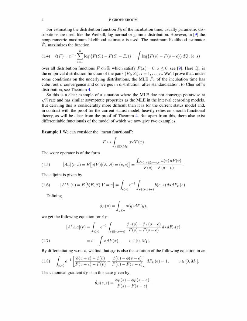
Example 1 We can consider the “mean functional”:

F 7→∫x∈[0,M1]

xdF (x)

The score operator is of the form

[Aa] (e, s) =E[a(V )|(E,S) = (e, s)

]=

∫v≥0, v∈(s−e,s] a(v)dF (v)

F (s)− F (s− e).(1.5)

The adjoint is given by

[A∗b] (v) =E[b(E,S)|V = v

]=

∫e>0

e−1∫s∈(v,v+e)

b(e, s)dsdFE(e).(1.6)

Defining

φF (u) =

∫y≤u

a(y)dF (y),

we get the following equation for φF :

[A∗Aa](v) =

∫e>0

e−1∫s∈(v,v+e)

φF (s)− φF (s− e)F (s)− F (s− e)

dsdFE(e)

= v−∫xdF (x), v ∈ [0,M1].(1.7)

By differentiating w.r.t. v, we find that φF is also the solution of the following equation in φ:∫e>0

e−1[φ(v+ e)− φ(v)

F (v+ e)− F (v)− φ(v)− φ(v− e)F (v)− F (v− e)

]dFE(e) = 1, v ∈ [0,M1].(1.8)

The canonical gradient θF is in this case given by:

θF (e, s) =φF (s)− φF (s− e)F (s)− F (s− e)

.

INCUBATION TIME 5

0 5 10 15 20

-2.5

-2.0

-1.5

-1.0

-0.5

0.0

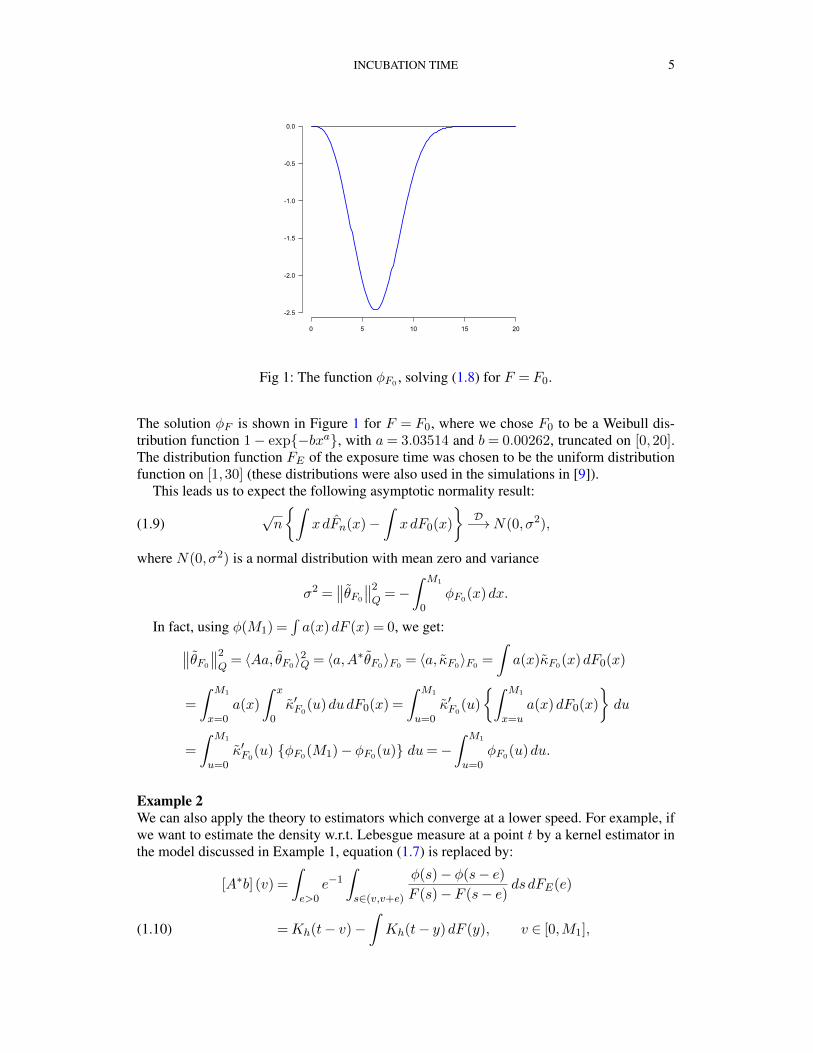
Fig 1: The function φF0, solving (1.8) for F = F0.

The solution φF is shown in Figure 1 for F = F0, where we chose F0 to be a Weibull dis-tribution function 1− exp{−bxa}, with a= 3.03514 and b= 0.00262, truncated on [0,20].The distribution function FE of the exposure time was chosen to be the uniform distributionfunction on [1,30] (these distributions were also used in the simulations in [9]).

This leads us to expect the following asymptotic normality result:√n

{∫xdFn(x)−

∫xdF0(x)

}D−→N(0, σ2),(1.9)

where N(0, σ2) is a normal distribution with mean zero and variance

σ2 =∥∥θF0

∥∥2Q

=−∫ M1

0φF0

(x)dx.

In fact, using φ(M1) =∫a(x)dF (x) = 0, we get:∥∥θF0

∥∥2Q

= 〈Aa, θF0〉2Q = 〈a,A∗θF0

〉F0= 〈a, κF0

〉F0=

∫a(x)κF0

(x)dF0(x)

=

∫ M1

x=0a(x)

∫ x

0κ′F0

(u)dudF0(x) =

∫ M1

u=0κ′F0

(u)

{∫ M1

x=ua(x)dF0(x)

}du

=

∫ M1

u=0κ′F0

(u) {φF0(M1)− φF0

(u)} du=−∫ M1

u=0φF0

(u)du.

Example 2We can also apply the theory to estimators which converge at a lower speed. For example, ifwe want to estimate the density w.r.t. Lebesgue measure at a point t by a kernel estimator inthe model discussed in Example 1, equation (1.7) is replaced by:

[A∗b] (v) =

∫e>0

e−1∫s∈(v,v+e)

φ(s)− φ(s− e)F (s)− F (s− e)

dsdFE(e)

=Kh(t− v)−∫Kh(t− y)dF (y), v ∈ [0,M1],(1.10)

6 P. GROENEBOOM

which becomes after differentiation w.r.t. v:

∫e>0

e−1[φ(v+ e)− φ(v)

F (v+ e)− F (v)− φ(v)− φ(v− e)F (v)− F (v− e)

]dFE(e) =−K ′h(t− v), v ∈ [0,M1],

(1.11)

where Kh(x) = h−1K(x/h) and K is a symmetric kernel with support [−1.1], for examplethe triweight kernel

K(x) =35

32

(1− x2

)31[−1,1](x).(1.12)

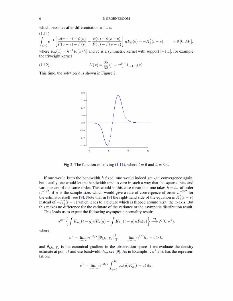
This time, the solution φ is shown in Figure 2.

0 5 10 15

-0.15

-0.10

-0.05

0.00

0.05

0.10

0.15

0.20

Fig 2: The function φ, solving (1.11), where t= 6 and h= 3.4.

If one would keep the bandwidth h fixed, one would indeed get√n convergence again,

but usually one would let the bandwidth tend to zero in such a way that the squared bias andvariance are of the same order. This would in this case mean that one takes h= hn of ordern−1/7, if n is the sample size, which would give a rate of convergence of order n−2/7 forthe estimator itself, see [9]. Note that in [9] the right-hand side of the equation is K ′h(t− v)instead of −K ′h(t− v) which leads to a picture which is flipped around w.r.t. the x-axis. Butthis makes no difference for the estimate of the variance or the asympotic distribution result.

This leads us to expect the following asymptotic normality result:

n2/7{∫

Khn(t− y)dFn(y)−

∫Khn

(t− y)dF0(y)

}D−→N(0, σ2),

where

σ2 = limn→∞

n−3/7∥∥θt,hn,F0

∥∥2Q, lim

n→∞n1/7hn = c > 0,

and θt,hn,F0is the canonical gradient in the observation space if we evaluate the density

estimate at point t and use bandwidth hn, see [9]. As in Example 1, σ2 also has the represen-tation:

σ2 = limn→∞

n−3/7∫ M1

u=0φn(u)K ′h(t− u)du,

INCUBATION TIME 7

where φn solves (1.11) for h= hn ∼ cn−1/7, for some c > 0.

The organization of the paper is as follows. In Section 2 we give necessary a sufficientconditions for Fn to be the MLE. Under some extra conditions, we derive consistency of theMLE in Section 3.

In Section 4 we discuss the limit distribution of the MLE. To our knowledge, this resulthas not been derived before. It is somewhat analogous to the methods, used in [7] for derivingthe asymptotic distribution of the MLE for the case of interval censoring, case 2 in Section4.2 of [7]. Although about 25 years have passed now since the publication of this proof, andalthough it would be nice to have a simpler proof of this result, no other proofs are known tome. So we have to go through similar but still somewhat different steps again.

In Section 5 we discuss the behavior of smooth estimates of the distribution function anddensity, based on the nonparametric MLE. We end with some concluding remarks in Section6. The Appendis, Section 7, contains technical details of the proof of the convergence of theMLE to Chernoff’s distribution.

2. Characterization of the nonparametric maximum likelihood estimator (MLE).Let Qn be the empirical distribution function of the pairs (Ei, Si). Then, for a distributionfunction F on R, which is zero on (−∞,0], we define the process

Wn,F (t) =

∫ {1− {s− e < t≤ s}

F (s)− F (s− e)

}dQn(e, s), t≥ 0,(2.1)

defining 0/0 = 0, where Qn is the empirical distribution of (E1, S1), . . . , (En, Sn). The fol-lowing lemma characterizes the MLE.

LEMMA 1. Let F be the set of discrete distribution functions with mass concentratedon a set of points Ti, i = 1, . . . ,m, where 0 < T1 < · · · < Tm and m ≥ 1. Then Fn ∈ Fmaximizes

`(F ) =

∫log{F (s)− F (s− e)}dQn(e, s)(2.2)

over F ∈ F if and only if

(i)

Wn,Fn(Tj)≥ 0, j = 1, . . . ,m,

(ii)

Wn,Fn(Tj) = 0, if Tj is a point of strictly positive mass of Fn.

PROOF. First suppose Fn satisfies (i) and (ii) and let pj = Fn(Tj) − Fn(Tj−1), j =1, . . . ,m, where T0 = 0. Then we have, using the concavity of the log function and Jensen’sinequality:

`(F )− `(Fn)

≤∫F (s)− F (s− e)− {Fn(s)− Fn(s− e)}

Fn(s)− Fn(s− e)dQn(e, s)

=

∫ ∫t∈(s−e,s] dF (t)−

∫t∈(s−e,s] dFn(t)

Fn(s)− Fn(s− e)dQn(e, s)

8 P. GROENEBOOM

=

∫ {1− {s− e < t≤ s}

Fn(s)− Fn(s− e)

}dQn(e, s)dFn(t)

−∫ {

1− {s− e < t≤ s}Fn(s)− Fn(s− e)

}dQn(e, s)dF (t)

=−∫ {

1− {s− e < t≤ s}Fn(s)− Fn(s− e)

}dQn(e, s)dF (t)≤ 0,

using (ii) and next (i) on the last line.Conversely, suppoe Fn ∈ F maximizes `(F ) over F . If Tj ∈ (Si −Ei, Si] we must have

Fn(Si)− Fn(Si −Ei)> 0, since otherwise `(Fn) =−∞. We have:

limε↓0

ε−1{`((Fn + ε1[Tj ,∞)

)/(1 + ε)

)− `(Fn)

}=

∫{s− e < Tj ≤ s}Fn(s)− Fn(s− e)

dQn(e, s)− 1 =Wn,Fn(Tj)≤ 0.

If Fn has mass at Ti, we also have:

limε↓0

ε−1{`((Fn − ε1[Tj ,∞)

)/(1− ε)

)− `(Fn)

}=−

∫{s− e < Tj ≤ s}Fn(s)− Fn(s− e)

dQn(e, s) + 1≤ 0,

and hence:

Wn,Fn(Tj) =

∫{s− e < Tj ≤ s}Fn(s)− Fn(s− e)

dQn(e, s)− 1 = 0.

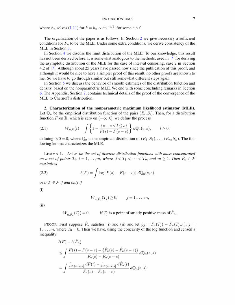
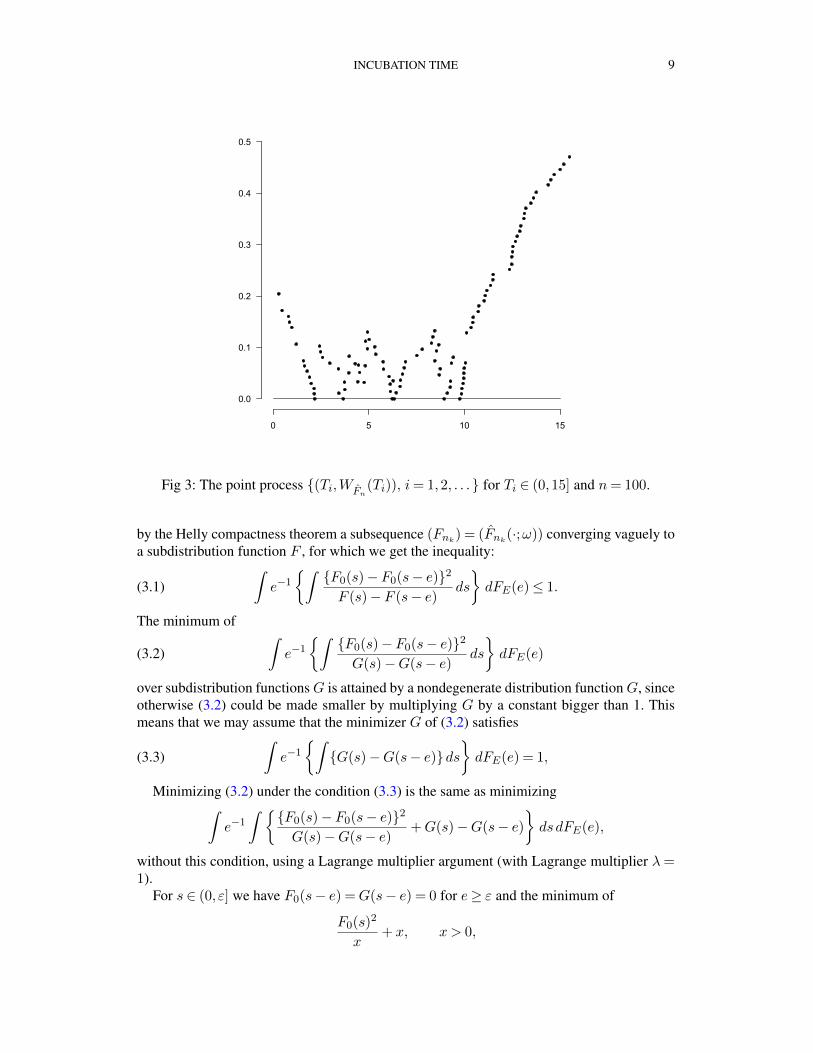
The lemma shows that the point process {(Ti,WFn(Ti)), i = 1,2, . . .} where Ti runs

through the ordered points Si and (Si − Ei)+, excluding 0, has second coordinates equalto 0 at points where the probability distribution, corresponding to Fn, has positive mass. Apicture of this point process is given in Figure 3 for sample size n= 100.

3. Consistency of the MLE. We have the following result.

THEOREM 3. Let F0 have a strictly positive density f0 on (0,M1), for some M1 > 0.Furthermore, let FE be zero on an interval [0, ε], where 0 < ε < M1 and have a strictlypositive continuous density fE on the interval (ε,M2). Let Fn ∈ Fn be the MLE, where Fn

is the set of distribution function with mass at the set of points Tj , where the Tj run throughthe ordered set of points Si and (Si −Ei)+, excluding the points (Si −Ei)+ = 0. Then theMLE Fn converges almost surely to F0 on [0,M1].

There are a lot of different ways to prove consistency, but we feel a preference for theelegant method in [14], which is used in the proof below.

PROOF. We start by observing that, by the fact that Fn is the MLE, we must have:∫F0(s)− F0(s− e)Fn(s)− Fn(s− e)

dQn(e, s)≤ 1.

On a set of probability one, the empirical probability measure Qn converges weakly to theunderlying measureQ0 on a set of elements ω which has probability one. Fixing and ω we get

INCUBATION TIME 9

0 5 10 15

0.0

0.1

0.2

0.3

0.4

0.5

Fig 3: The point process {(Ti,WFn(Ti)), i= 1,2, . . .} for Ti ∈ (0,15] and n= 100.

by the Helly compactness theorem a subsequence (Fnk) = (Fnk

(·;ω)) converging vaguely toa subdistribution function F , for which we get the inequality:∫

e−1{∫

{F0(s)− F0(s− e)}2

F (s)− F (s− e)ds

}dFE(e)≤ 1.(3.1)

The minimum of ∫e−1

{∫{F0(s)− F0(s− e)}2

G(s)−G(s− e)ds

}dFE(e)(3.2)

over subdistribution functionsG is attained by a nondegenerate distribution functionG, sinceotherwise (3.2) could be made smaller by multiplying G by a constant bigger than 1. Thismeans that we may assume that the minimizer G of (3.2) satisfies∫

e−1{∫{G(s)−G(s− e)}ds

}dFE(e) = 1,(3.3)

Minimizing (3.2) under the condition (3.3) is the same as minimizing∫e−1

∫ {{F0(s)− F0(s− e)}2

G(s)−G(s− e)+G(s)−G(s− e)

}dsdFE(e),

without this condition, using a Lagrange multiplier argument (with Lagrange multiplier λ=1).

For s ∈ (0, ε] we have F0(s− e) =G(s− e) = 0 for e≥ ε and the minimum of

F0(s)2

x+ x, x > 0,

10 P. GROENEBOOM

is attained by taking x= F0(s). If F0(s)>F0(s− e)> 0, we find that

{F0(s)− F0(s− e)}2

y− x+ y− x, x≥ 0, y− x > 0,

is minimized by taking y−x= F0(s)−F0(x), but since the minimizing values on the intervalu ∈ (0, ε] are equal F0(u), we must have G(s) = F0(s) and G(s− e) = F0(x− e) for theminimizing function G.

So the minimum of (3.2) is equal to 1 and attained for G= F0. This means that the limitF the subsequence (Fnk

) must be equal to F0, since otherwise the left-hand side of (3.1)would be strictly bigger than 1. Since this holds for all subsequences (Fnk

), the result nowfollows.

4. Asymptotic distribution of the MLE. In this section we discuss the proof of thetheorem below.

THEOREM 4. Let F0 have a continuous density f0, staying away from zero on its support[0,M1], M1 > 0, and let the exposure time E have a continuous density fE ≥ c > 0 onits support [ε,M2], for some c > 0, with a bounded derivative on the interval (ε,M2). LetFn ∈ Fn be the MLE, where the set of distribution functions Fn has the same meaning as inTheorem 3. Then we have at a point t0 ∈ (0,M1):

n1/3{Fn(t0)− F0(t0)}/(4f0(t0)/cE)1/3d−→ argmin

{W (t) + t2

},(4.1)

where W is two-sided Brownian motion on R, originating from zero and where the constantcE is given by:

cE =

∫e−1

[1

F0(t0)− F0(t0 − e)+

1

F0(t0 + e)− F0(t0)

]dFE(e),(4.2)

The result shows that the limit distribution is given by Chernoff’s distribution. This distri-bution also occurs as limit distribution in the current status model and more generally in theinterval censoring model in the so-called separated case, The jump in difficulty of the proofin going from the result for the current status model to the interval censoring, case 2, modelis considerable. Similarly the present proof is not simple. The proofs of the lemma’s will begiven in the Appendix.

We have the following lemma.

LEMMA 2. Let, under the conditions of Theorem 4, the process Xn be defined by:

Xn(t) =

∫{s− e < t0 ≤ s}Fn(s)− Fn(s− e)

d(Qn −Q0

)(e, s)

−∫{s− e < t0 + n−1/3t≤ s}

Fn(s)− Fn(s− e)d(Qn −Q0

)(e, s).

Let t0 be an interior point of the support of f0. Then n2/3Xn converges in distribution, in theSkorohod topology, to the process

t 7→√cEW (t), t ∈R,

where cE and W are the same as in Theorem 4.

We also have the following property of the MLE.

INCUBATION TIME 11

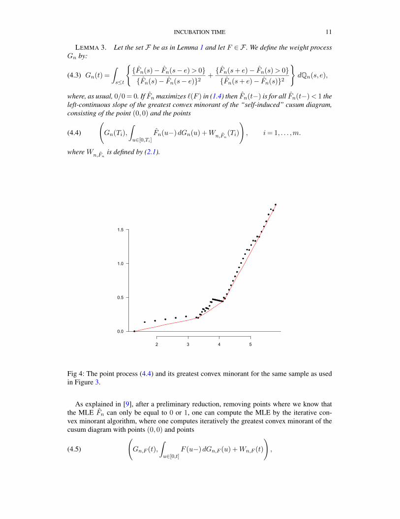
LEMMA 3. Let the set F be as in Lemma 1 and let F ∈ F . We define the weight processGn by:

Gn(t) =

∫s≤t

{{Fn(s)− Fn(s− e)> 0}{Fn(s)− Fn(s− e)}2

+{Fn(s+ e)− Fn(s)> 0}{Fn(s+ e)− Fn(s)}2

}dQn(s, e),(4.3)

where, as usual, 0/0 = 0. If Fn maximizes `(F ) in (1.4) then Fn(t−) is for all Fn(t−)< 1 theleft-continuous slope of the greatest convex minorant of the “self-induced” cusum diagram,consisting of the point (0,0) and the points(

Gn(Ti),

∫u∈[0,Ti]

Fn(u−)dGn(u) +Wn,Fn(Ti)

), i= 1, . . . ,m.(4.4)

where Wn,Fnis defined by (2.1).

2 3 4 5

0.0

0.5

1.0

1.5

Fig 4: The point process (4.4) and its greatest convex minorant for the same sample as usedin Figure 3.

As explained in [9], after a preliminary reduction, removing points where we know thatthe MLE Fn can only be equal to 0 or 1, one can compute the MLE by the iterative con-vex minorant algorithm, where one computes iteratively the greatest convex minorant of thecusum diagram with points (0,0) and points(

Gn,F (t),

∫u∈[0,t]

F (u−)dGn,F (u) +Wn,F (t)

),(4.5)

12 P. GROENEBOOM

where Gn,F is defined as in (4.3), but with Fn replaced by F , where F is the temporary esti-mate of the distribution function at an iteration, and where t runs through the order statisticsof the observations Si and (Si −Ei)+ (excluding zero). The MLE Fn corresponds to a sta-tionary point of this algorithm and is given by the left-continuous slope of the greatest convexminorant of the cusum diagram, see Figure 4. See [9] for further remarks on this algorithm.

A fundamental tool in our proof is the so-called “switch relation”, see, e.g., Section 3.8 in[10]. Let the process Vn be defined by

Vn(t) =

∫u∈[0,t]

Fn(u−)dGn(u) +Wn,Fn(t),(4.6)

where Gn is the function, defined by (4.3) at the points Ti and extended to a right-continuouspiecewise constant function elsewhere. We define, for a ∈ (0,1)

Un(a) = argmin{t ∈ [0,∞) : Vn(t)− aGn(t)}.

Then we have the switch relation:

Fn(t)≥ a ⇐⇒ Gn(t)≥Gn(Un(a)) ⇐⇒ t≥ Un(a).

see, e.g., (3.35) and Figure 3.7 in Section 3.8 of [10].We have:

P{n1/3

{Fn(t0)− F0(t0)

}≥ x}

= P{n1/3

{Un(a0 + n−1/3x)− t0

}≤ 0},

where a0 = F0(t0). Using the property that the argmin function does not change if we addconstants to the object function, we get:

Un(a0 + n−1/3x) = argmin{t ∈ [0,∞) : Vn(t)−

(a0 + n−1/3x

)Gn(t)

}= argmin

{t ∈ [0,∞) : Vn(t)− Vn(t0)−

(a0 + n−1/3x

){Gn(t)−Gn(t0)

}}= argmin

{t0 + n−1/3t≥ 0 :

∫u∈(t0,t0+n−1/3t]

Fn(u−)dGn(u)

+Wn,Fn(t0 + n−1/3t)−Wn,Fn

(t0)

− n−1/3x{Gn(t0 + n−1/3t)−Gn(t0)

}},

where ∫u∈(t,v]

Fn(u−)dGn(u) =−∫u∈[v,t)

Fn(u−)dGn(u), if v < t.

We have:

Wn,Fn(t0 + n−1/3t)

=Xn(t) +

∫{s− e < t0 ≤ s}F0(s)− F0(s− e)

dQ0(e, s)−∫{s− e < t0 + n−1/3t≤ s}

F0(s)− F0(s− e)dQ0(e, s),

where Xn is given in Lemma 2. For the second part in the last expression we have the fol-lowing result.

INCUBATION TIME 13

LEMMA 4. Let the conditions of Theorem 4 be satisfied. Then, for arbitrary M > 0 andt ∈ [−M,M ]:∫

s∈(t0,t0+n−1/3t]

{Fn(s−)− F0(t0)

}dGn(u)

+

∫{s− e < t0 ≤ s}Fn(s)− Fn(s− e)

dQ0(e, s)−∫{s− e < t0 + n−1/3t≤ s}

Fn(s)− Fn(s− e)dQ0(e, s)

= 12f0(t0)cEn

−2/3t2 +Bn + op

(n−2/3

),

where

Bn

=

∫e−1

∫s∈[t0,t0+n−1/3t)

{Fn(s− e)− F0(s− e)Fn(s)− Fn(s− e)

+Fn(s+ e)− F0(s+ e)

Fn(s+ e)− Fn(s)

}dsdFE(e).

We will also need the following rate result for the L2-distance.

LEMMA 5. Let the conditions of Theorem 4 be satisfied.. Then

‖Fn − F0‖=Op

(n−1/3

).(4.7)

The term Bn in Lemma 4 is now treated by using differentiable functional theory, asdiscussed in the Introduction. We really have to use smooth functional theory here and cannotuse simple L2-bounds or other tools of that type only to show that Bn is of order op(n−2/3).One could say that this is the heart of the difficulty of the proof. We have:

LEMMA 6. Let the conditions of Theorem 4 be satisfied. Then, for arbitrary M > 0 andt ∈ [−M,M ]:

Bn =Op

(n−5/6

).

A slightly more general result of the same type is that∫s∈[t,u]

∫e−1

{Fn(s− e)− F0(s− e)Fn(s)− Fn(s− e)

+Fn(s+ e)− F0(s+ e)

Fn(s+ e)− Fn(s)

}dFE(e)ds

=Op

((u− t)n−1/2

)+Op

(n−5/6

),(4.8)

for intervals [t, u] such that 0< t < u<M1.We also need the following upper bound,

LEMMA 7. Let the conditions of Theorem 4 be satisfied. Then

supx∈[0,M1]

∣∣∣Fn(x)− F0(x)∣∣∣=Op

(n−1/4

).

We finally need the following “tightness” lemma.

14 P. GROENEBOOM

LEMMA 8. Let the conditions of Theorem 4 be satisfied and let a0 ∈ (0,1). Then, foreach δ > 0 and K1 > 0 a K2 > 0 can be found such that

P

{sup

x∈[−K1,K1]n1/3

{Un

(a0 + n−1/3x

)− t0

}>K2

}< δ,

and

P{

infx∈[−K1,K1]

n1/3{Un

(a0 + n−1/3x

)− t0

}<−K2

}< ε,

for all large n.

We now have:

n1/3{Un(a0 + n−1/3x)− t0

}= argmin

{t≥−n2/3t0 : n2/3Xn(t) + 1

2cEf0(t0)t2 − n1/3x

{Gn(t0 + n−1/3t)−Gn(t0)

}+ op(1)

}

= argmin

{t≥−n2/3t0 : n2/3Xn(t) + 1

2cEf0(t0)t2 − cExt+ op(1)

},

which converges in distribution to the argmin of the process

t 7→√cEW (t) + 1

2cEf0(t0)t2 − cExt, t ∈R,

whereW is two-sided Brownian motion, originating from zero. Theorem 4 now follows fromBrownian scaling.

0 2 4 6 8 10 12 14

0.0

0.2

0.4

0.6

0.8

1.0

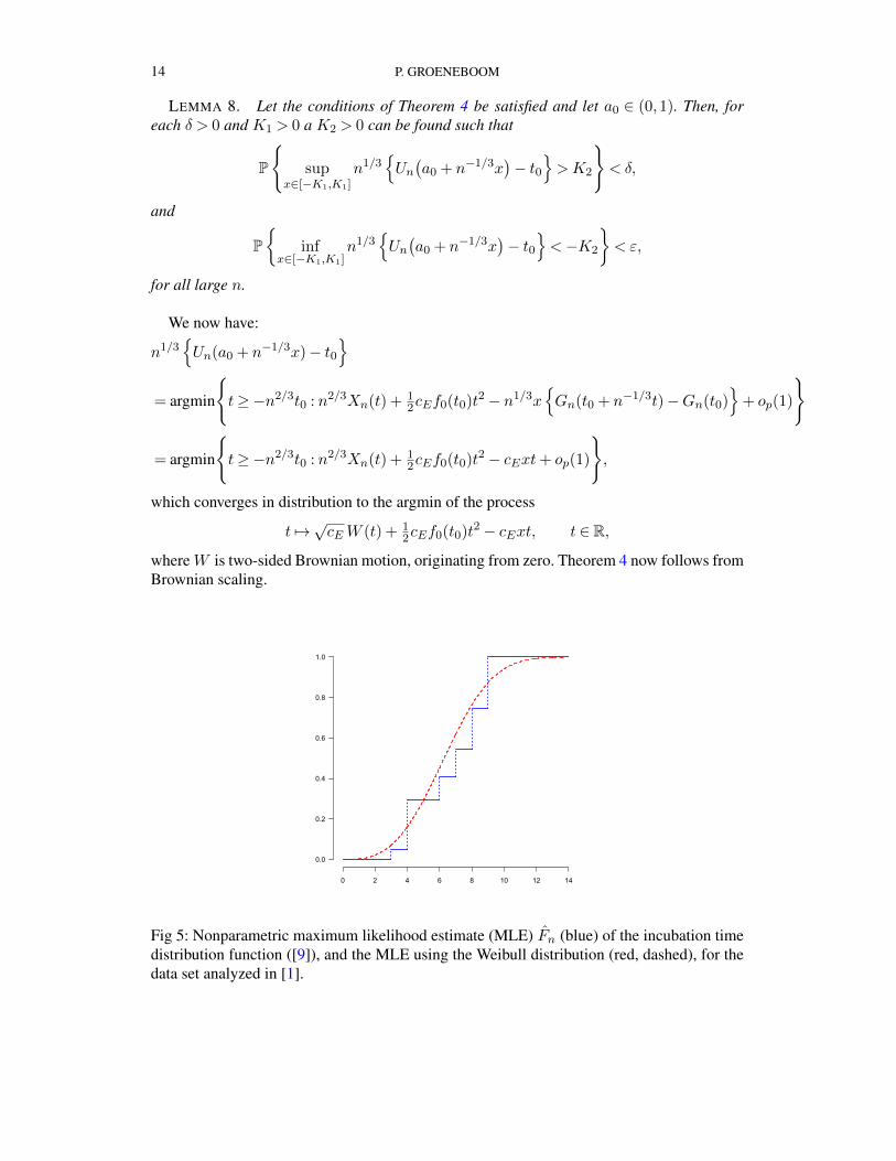
Fig 5: Nonparametric maximum likelihood estimate (MLE) Fn (blue) of the incubation timedistribution function ([9]), and the MLE using the Weibull distribution (red, dashed), for thedata set analyzed in [1].

INCUBATION TIME 15

5. Estimates of differentiable functionals. The data of 81 travelers from Wuhan wereanalyzed in connection with the start of the COVID-19 pandemic ([1]). One can maximize

`(F ) =

n∑i=1

log{F (Si)− F (Si −Ei)

]over Weibull distribtions F (or other distributions of that type), as is done in [1]

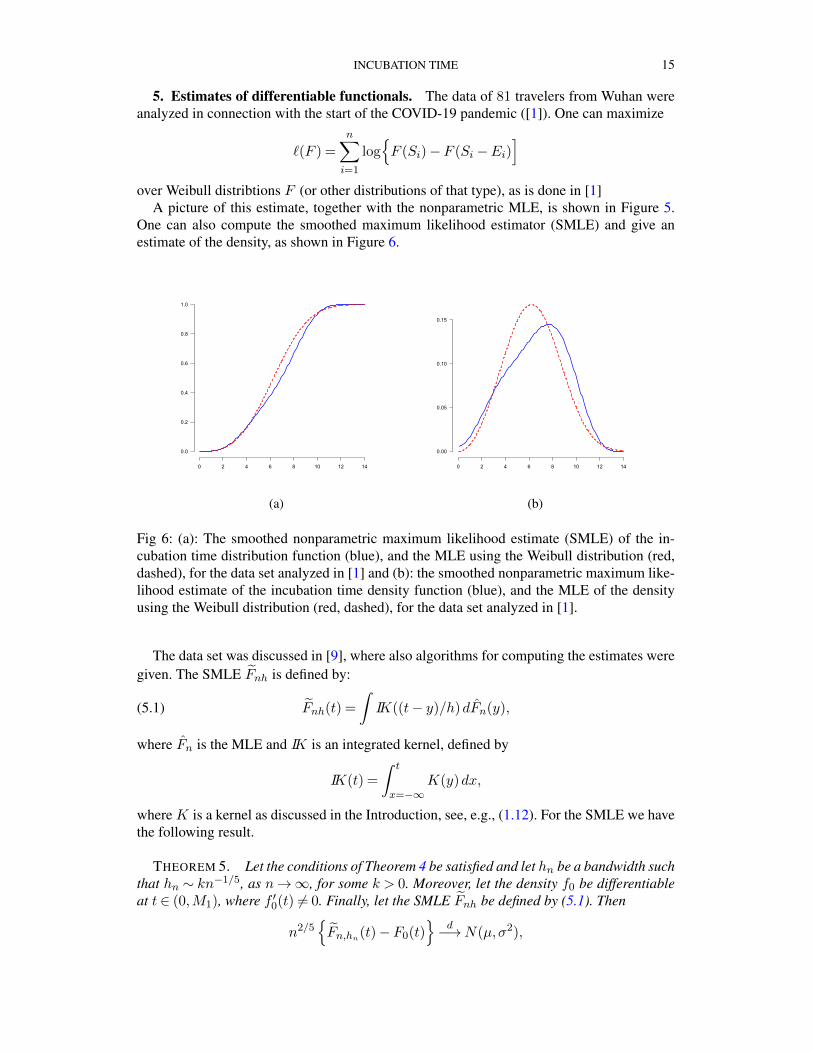
A picture of this estimate, together with the nonparametric MLE, is shown in Figure 5.One can also compute the smoothed maximum likelihood estimator (SMLE) and give anestimate of the density, as shown in Figure 6.

0 2 4 6 8 10 12 14

0.0

0.2

0.4

0.6

0.8

1.0

(a)

0 2 4 6 8 10 12 14

0.00

0.05

0.10

0.15

(b)

Fig 6: (a): The smoothed nonparametric maximum likelihood estimate (SMLE) of the in-cubation time distribution function (blue), and the MLE using the Weibull distribution (red,dashed), for the data set analyzed in [1] and (b): the smoothed nonparametric maximum like-lihood estimate of the incubation time density function (blue), and the MLE of the densityusing the Weibull distribution (red, dashed), for the data set analyzed in [1].

The data set was discussed in [9], where also algorithms for computing the estimates weregiven. The SMLE Fnh is defined by:

Fnh(t) =

∫IK((t− y)/h)dFn(y),(5.1)

where Fn is the MLE and IK is an integrated kernel, defined by

IK(t) =

∫ t

x=−∞K(y)dx,

where K is a kernel as discussed in the Introduction, see, e.g., (1.12). For the SMLE we havethe following result.

THEOREM 5. Let the conditions of Theorem 4 be satisfied and let hn be a bandwidth suchthat hn ∼ kn−1/5, as n→∞, for some k > 0. Moreover, let the density f0 be differentiableat t ∈ (0,M1), where f ′0(t) 6= 0. Finally, let the SMLE Fnh be defined by (5.1). Then

n2/5{Fn,hn

(t)− F0(t)}

d−→N(µ,σ2),

16 P. GROENEBOOM

where

µ= 12k

2f ′0(t)

∫u2K(u)du,(5.2)

and

σ2 = limn→∞

n−1/5∫φn,F0

(y)Khn(t− y)dy(5.3)

where the function φn,F0solves the equation

∫e>0

e−1[φ(v+ e)− φ(v)

F0(v+ e)− F0(v)− φ(v)− φ(v− e)F0(v)− F0(v− e)

]dFE(e) =−Khn

(t− v), v ∈ (0,M1).

(5.4)

PROOF. This time the adjoint equation is (for Fn instead of F0):

[A∗b] (v) =

∫e>0

e−1∫s∈(v,v+e)

φ(s)− φ(s− e)Fn(s)− Fn(s− e)

dsdFE(e)

= IK((t− v)/hn)−∫Kh((t− y)/hn)dFn(y), v ∈ (0,M1).(5.5)

We have, for all large n:∫IK(t− v)/hn)d

(Fn − F0

)(v)

=

∫ ∫e>0

e−1∫s∈(v,v+e)

φn(s)− φn(s− e)Fn(s)− Fn(s− e)

dsdFE(e)d(Fn − F0

)(v)

=−∫e>0

e−1∫ [

φn(v+ e)− φn(v)

Fn(v+ e)− Fn(v)− φ(v)− φ(v− e)Fn(v)− Fn(v− e)

](Fn − F0

)(v)dv dFE(e),

where the last equality follows from integration by parts, and where φn = φn,Fnis a solution

of (5.5). So we get:∫IK(t− v)/hn)d

(Fn − F0

)(v)

=−∫e>0

e−1∫ {

Fn(s)− F0(s)}[φn(s+ e)− φn(s)

Fn(s+ e)− Fn(s)− φn(s)− φn(s− e)Fn(s)− Fn(s− e)

]dsdFE(e)

=−∫e>0

e−1∫ {

Fn(s)− Fn(s− e)− F0(s) + F0(s− e)} φn(s)− φn(s− e)Fn(s)− Fn(s− e)

dsdFE(e)

=

∫e>0

e−1∫{F0(s)− F0(s− e)}

φn(s)− φn(s− e)Fn(s)− Fn(s− e)

dsdFE(e)

=

∫φn(s)− φn(s− e)Fn(s)− Fn(s− e)

dQ0(e, s).

Replacing φn by a piecewise constant function φn, absolutely continuous w.r.t. Fn, in thesame way as is done on p. 290 of [10], we find∣∣∣∣∫ φn(s)− φn(s− e)

Fn(s)− Fn(s− e)dQ0(e, s)−

∫φn(s)− φn(s− e)Fn(s)− Fn(s− e)

dQ0(e, s)

∣∣∣∣

INCUBATION TIME 17

=

∣∣∣∣∫e>0

e−1∫ {

Fn(s)− Fn(s− e)− F0(s) + F0(s− e)}

· φn(s)− φn(s)− φn(s− e) + φn(s− e)Fn(s)− Fn(s− e)

dsdFE(e)

∣∣∣∣. ‖Fn − F0‖2‖φn − φn‖2 ==Op

(h−1n n−2/3

)=Op

(n−7/15

)= op

(n−2/5

),

using Lemma 5 and the arguments on p. 333 of [10] (see in particular (11.49)). Moreover,∫φn(s)− φn(s− e)Fn(s)− Fn(s− e)

dQn(e, s) = 0.

Thus we find: ∫IK(t− v)/hn)d

(Fn − F0

)(v)

=

∫φn(s)− φn(s− e)Fn(s)− Fn(s− e)

dQ0(e, s)

=

∫φn(s)− φn(s− e)Fn(s)− Fn(s− e)

dQ0(e, s) + op

(n−2/5

)=−

∫φn(s)− φn(s− e)Fn(s)− Fn(s− e)

d(Qn −Q0

)(e, s) + op

(n−2/5

)=−

∫φn(s)− φn(s− e)Fn(s)− Fn(s− e)

d(Qn −Q0

)(e, s) + op

(n−2/5

).

Finally,

n2/5∫IK(t− v)/hn)d

(Fn − F0

)(v)

∼−n2/5∫φn(s)− φn(s− e)Fn(s)− Fn(s− e)

d(Qn −Q0

)(e, s)

=−n2/5∫φn,F0

(s)− φn,F0(s− e)

F0(s)− F0(s− e)d(Qn −Q0

)(e, s) + op(1)

=−n2/5∫θn,F0

(e, s)d(Qn −Q0

)(e, s) + op(1),

where θn,F0is the canonical gradient, and the asymptotic variance σ2is therefore given by

limn→∞

n−1/5‖θn,F0‖2Q0

= limn→∞

n−1/5∫φn,F0

(u)Khn(u)du.

The expression (5.2) for µ arises from the expansion of the bias∫IK(t− y)dF0(y)− F0(t).

We likewise have:

18 P. GROENEBOOM

THEOREM 6. Let the conditions of Theorem 4 be satisfied and let hn be a bandwidthsuch that hn ∼ kn−1/7, as n→∞, for some k > 0. Moreover, let the density f0 be twicedifferentiable at t ∈ (0,M1), where f ′′0 (t) 6= 0. Finally, let the density estimate fnh(t) bedefined by

fnh(t) =

∫Kh(t− y)dFn(y),

where Fn is the MLE. Then

n2/7{fn,hn

(t)− f0(t)}

d−→N(µ,σ2),

where

µ= 12k

2f ′′0 (t)

∫u2K(u)du,(5.6)

and

σ2 = limn→∞

n−3/7∫φn,F0

(y)K ′hn(t− y)dy,(5.7)

where the function φn,F0solves the equation

∫e>0

e−1[φ(v+ e)− φ(v)

F0(v+ e)− F0(v)− φ(v)− φ(v− e)F0(v)− F0(v− e)

]dFE(e) =−K ′hn

(t− v), v ∈ (0,M1).

(5.8)

The proof proceeds along similar lines as the proof of Theorem 5, where we use equation(5.8) this time, as mentioned in the Introduction (see (1.11)). The rather good fit of simula-tions of the variance with the theoretical expressions of type (5.7) was discussed in [9].

Finally, results of type (1.9) for moment type functionals can again be proved in a similarway. See for other results of type (1.9) Chapter 10 of [10].

6. Conclusion. We proved that the nonparametric MLE in an often used model for theincubation time distribution converges in distribution, after standardization, to Chernoff’sdistribution. The rate of convergence is cube root n, if n is the sample size. We also dis-cussed differentiable functionals of the model, estimated by corresponding functionals of thenonparametric MLE, which converge after standardization to a normal distribution, wherethe constants are given by the solutions of integral equations.

This provides an alternative for the parametric models which are usually applied in thiscontext, estimating the incubaton time distribution by, e.g., Weibull, gamma or log-normaldistributions. The latter methods will not be able to catch finer aspects of the data, in contrastwith, for example, the nonparametric density estimates, discussed in this paper.

There is also something deeply unsatisfactory in having to use several parametric distribu-tions in the estimating procedure, because there is no compelling reason to use one of these.Unlike the situation where one has convergence to a universal distribution, like the normaldistribution or Chernoff’s distribution in the so-called non-standard asymptotics case. More-over, these parametric distribution estimates will generally be inconsistent, in contrast withthe nonparametric estimates (as proved in the present paper).R scripts for computing the estimates are given in [8].

INCUBATION TIME 19

7. Appendix.

PROOF OF LEMMA 2. This follows from the convergence to the same limit process of∫{s− e < t0 ≤ s}F0(s)− F0(s− e)

d(Qn −Q0

)(e, s)−

∫{s− e < t0 + n−1/3t≤ s}

F0(s)− F0(s− e)d(Qn −Q0

)(e, s),

and the consistency of Fm together with the entropy with bracketing for the L2-norm of thefunctions

(e, s) 7→ 1

F (s)− F (s− e), s ∈ [t0 − n−1/3M,t0 + n−1/3M ], e≥ ε,

for M > 0 and distribution functions F such that {F (s)−F (s− e)}1{e≥ε} stays away fromzero for s in the relevant interval (see, e.g., p. 59, 59 of [10]).

PROOF OF LEMMA 3. We use the characterization of Lemma 1. Let Tj be the leftmostpoint of mass of Fn. Then Wn,Fn

(Tj) = 0. Since also Fn(Tj−) = 0 and, by monotonicity,

Fn(Ti−) = 0 for all Ti < Tj , the second coordinate of the cusum diagram is zero at Tj . IfTk is the second point of mass from the left, the slope of the greatest convex minorant isFn(Tk−) on (Gn(Ti),Gn(Tk)]. This can be continued up to the rightmost point T`, wherethe distribution corresponding to Fn has mass.

PROOF OF LEMMA 4. We have:∫{s− e < t0 ≤ s}Fn(s)− Fn(s− e)

dQ0(e, s)−∫{s− e < t0 + n−1/3t≤ s}

Fn(s)− Fn(s− e)dQ0(e, s)

=

∫e−1

∫s∈[t0,t0++n−1/3t)

F0(s)− F0(s− e)Fn(s)− Fn(s− e)

dsdFE(e)

−∫e−1

∫s∈[t0+e,t0+e+n−1/3t)

F0(s)− F0(s− e)Fn(s)− Fn(s− e)

dsdFE(e)

=

∫e−1

∫s∈[t0,t0+n−1/3t)

{F0(s)− F0(s− e)Fn(s)− Fn(s− e)

− F0(s+ e)− F0(s)

Fn(s+ e)− Fn(s)

}dsdFE(e)

=

∫e−1

∫s∈[t0,t0+n−1/3t)

F0(s)− F0(s− e)− Fn(s) + Fn(s− e)Fn(s)− Fn(s− e)

dsdFE(e)

−∫e−1

∫s∈[t0,t0+n−1/3t)

F0(s+ e)− F0(s)− Fn(s+ e) + Fn(s)

Fn(s+ e)− Fn(s)dsdFE(e).

The last expression can be rewritten in the form An +Bn, where

An

=−∫e−1

∫s∈[t0,t0+n−1/3t)

{Fn(s)− F0(s)

}{ 1

Fn(s)− Fn(s− e)+

1

Fn(s+ e)− Fn(s)

}dsdFE(e),

and

Bn

=

∫e−1

∫s∈[t0,t0+n−1/3t)

{Fn(s− e)− F0(s− e)Fn(s)− Fn(s− e)

+Fn(s+ e)− F0(s+ e)

Fn(s+ e)− Fn(s)

}dsdFE(e).

20 P. GROENEBOOM

We also have:∫s∈(t0,t0+n−1/3t]

Fn(s−)dGn(s)− a0{Gn(t0 + n−1/3t)−Gn(t0)

}=

∫s∈(t0,t0+n−1/3t]

{Fn(s)− F0(t0)

{Fn(s)− Fn(s− e)}2+

Fn(s)− F0(t0)

{Fn(s+ e)− Fn(s)}2

}dQn(s, e)

=

∫s∈(t0,t0+n−1/3t]

{Fn(s)− F0(s)

{Fn(s)− Fn(s− e)}2+

Fn(s)− F0(s)

{Fn(s+ e)− Fn(s)}2

}dQn(s, e)

+

∫s∈(t0,t0+n−1/3t]

{F0(s)− F0(t0)

{Fn(s)− Fn(s− e)}2+

F0(s)− F0(t0)

{Fn(s+ e)− Fn(s)}2

}dQn(s, e)

=

∫s∈(t0,t0+n−1/3t]

{Fn(s)− F0(s)

{Fn(s)− Fn(s− e)}2+

Fn(s)− F0(s)

{Fn(s+ e)− Fn(s)}2

}dQn(s, e)

+ 12cEf0(t0)t

2 + op

(n−2/3

)=−An + 1

2cEf0(t0)n−2/3t2 + op

(n−2/3

),

where cE is given by (4.2). This is seen by writing∫s∈(t0,t0+n−1/3t]

{Fn(s)− F0(s)

{Fn(s)− Fn(s− e)}2+

Fn(s)− F0(s)

{Fn(s+ e)− Fn(s)}2

}dQn(s, e)

=

∫s∈(t0,t0+n−1/3t]

{Fn(s)− F0(s)

{Fn(s)− Fn(s− e)}2+

Fn(s)− F0(s)

{Fn(s+ e)− Fn(s)}2

}d(Qn −Q0

)(s, e)

+

∫s∈(t0,t0+n−1/3t]

{Fn(s)− F0(s)

{Fn(s)− Fn(s− e)}2+

Fn(s)− F0(s)

{Fn(s+ e)− Fn(s)}2

}dQ0(s, e)

=−An + op

(n−2/3

),

using the consistency of Fn to show that the first term after the next to last equality is of orderop(n−2/3

). The result now follows.

PROOF OF LEMMA 5. We define the (convolution) density qF by (1.3). We now followthe exposition in the related model of interval censoring, case 2, in [18], Example 7.4.4. Thecondition that the exposure time E stays away from zero is comparable to the condition (7.4)on p. 16 of [18] that the intervals [U,V ] have a length which stays away from zero. In thiscase we find that the squared Hellinger distance satisfies:

h(qFn

, qF0

)2= 1

2

∫ {√qFn−√qF0

}2dsdFE(e)

= 12

∫e∈[ε,M2]

e−1∫s∈[0,M1+M2]

{√Fn(s)− Fn(s− e)−

√F0(s)− F0(s− e)

}2

dsdFE(e)

=Op

(n−2/3

),

see (7.42) in [18].

INCUBATION TIME 21

By the assumptions on the underlying distributions this also implies that∫e∈[ε,M2]

∫s∈[0,M1+M2]

{√Fn(s)− Fn(s− e)−

√F0(s)− F0(s− e)

}2

dsde

=Op

(n−2/3

),

and by the relation

(a− b)2 ={√

a−√b}2{√

a+√b}2≤ 2

{√a−√b}2

, a, b ∈ [0,1],

this implies{∫e∈[ε,M2]

∫s∈[0,M1+M2]

{Fn(s)− Fn(s− e)− F0(s) + F0(s− e)

}2dsde

}1/2

=Op

(n−1/3

).

We now partition the integration interval [0,M1 +M2] for s into a finite number of intervalsof length at most ε: [0, ε], ε,2ε], . . . , [kε,M1 +M2]. For s ∈ [0, ε] we get:{∫

e∈[ε,M2]

∫s∈[0,ε]

{Fn(s)− Fn(s− e)− F0(s) + F0(s− e)

}2dsde

}1/2

=

{(M2 − ε)

∫s∈[0,ε]

{Fn(s)− F0(s)

}2ds

}1/2

= (M2 − ε)1/2∥∥∥(Fn − F0

)1s∈[0,ε]

∥∥∥2

=Op

(n−1/3

).

For s ∈ [ε,2ε] we get:{∫u∈[0,ε]

∫s∈[ε,2ε]

{Fn(s)− Fn(u)− F0(s) + F0(u)

}2dsdu

}1/2

≤

{∫e∈[ε,M2]

∫s∈[ε,2ε]

{Fn(u)− F0(u)

}2dsdu

}1/2

=Op

(n−1/3

),

Introducing the L2-norm

‖h}=

{∫h(u, v)2 dudv

}1/2

for functions on R2, we get by the triangle inequality

√ε

{∫s∈[ε,2ε]

{Fn(s)− F0(s)

}2ds

}1/2

=

{∫u∈[0,ε]

∫s∈[ε,2ε]

{Fn(s)− F0(s)

}2dsdu

}1/2

22 P. GROENEBOOM

≤

{∫u∈[0,ε]

∫s∈[ε,2ε]

{Fn(s)− Fn(u)− F0(s) + F0(u)

}2dsdu

}1/2

+

{∫u∈[0,ε]

∫s∈[ε,2ε]

{Fn(u)− F0(u)

}2dsdu

}1/2

=Op

(n−1/3

).

Continuing this procedure on the next intervals [kε, (k + 1)ε] we get from the triangle in-equation for l2-norms:{∫

s∈[0,M1]

{Fn(s)− F0(s)

}2ds

}1/2

=Op

(n−1/3

).

PROOF OF LEMMA 6. We consider for s ∈ [t0, t0 + n−1/3t).the integral equations∫e>0

e−1[φ(v+ e)− φ(v)

Fn(v+ e)− Fn(v)− φ(v)− φ(v− e)Fn(v)− Fn(v− e)

]fE(e)de

= 1[0,s−ε)(v)fE(s− v){

Fn(s)− Fn(v)}

(s− v).(7.1)

Let

gs(v) = 1[0,s−ε)(v)fE(s− v){

Fn(s)− Fn(v)}

(s− v),(7.2)

and let φs be the solution of the integral equation in φ. The proof of the existence and unique-ness of the solution follows the lines of the proofs for similar equations in [7]. We have:∫

e−1Fn(s− e)− F0(s− e)Fn(s)− Fn(s− e)

dFE(e)

=

∫1[0,s−ε)(v)

fE(s− v){Fn(s)− Fn(v)

}(s− v)

{Fn(v)− F0(v)

}dv

=

∫gs(v)

{Fn(v)− F0(v)

}dv

=

∫{Fn(v)− F0(v)}

∫e>0

e−1[φs(v+ e)− φs(v)

Fn(v+ e)− Fn(v)− φs(v)− φs(v− e)Fn(v)− Fn(v− e)

]dFE(e)dv

=−∫{Fn(v)− Fn(v− e)− F0(v) + F0(v− e)}

∫e>0

e−1φs(v)− φs(v− e)Fn(v)− Fn(v− e)

dFE(e)dv

=

∫φs(v)− φs(v− e)Fn(v)− Fn(v− e)

dQ0(e, v) =

∫θg,Fn

dQ0(e, v).

where Q0 is the probability measure on the observation space, noting that∫{Fn(v)− Fn(v− e)}

∫e>0

e−1φs(v)− φs(v− e)Fn(v)− Fn(v− e)

dFE(e)dv

=

∫e>0

e−1∫ {

φs(v)− φs(v− e)}dv dFE(e) = 0.

INCUBATION TIME 23

We can replace φs by a piecewise constant function φs, absolutely continuous w.r.t. Fn,leading to gradient θg,Fn

in a similar way as done, for example, in the proof of Lemma 4.4on p. 146 of [7]. For this replacement we get∫

θg,FndQ0(e, v) =

∫θg,Fn

dQ0(e, v) +Op

(n−2/3

)=−

∫θg,Fn

d (Qn −Q0) (e, v) +Op

(n−2/3

)So the conclusion is:∫

e−1Fn(s− e)− F0(s− e)Fn(s)− Fn(s− e)

dFE(e) =−∫θg,Fn

d (Qn −Q0) (e, v) +Op

(n−2/3

)=Op

(n−1/2

).

Similarly: ∫e−1

Fn(s+ e)− F0(s+ e)

Fn(s)− Fn(s− e)dFE(e) =Op

(n−1/2

).

Since, just as in [7] these terms are Op

(n−1/2

)uniform in s ∈ [t0, t0 + n−1/3t), we can

conclude that

Bn =Op

(n−5/6

).

The extension to (4.8) is straightforwward.

PROOF OF LEMMA 7. The proof is analogous to the proof of Corollary 4.4 in [7], whichuses

supt∈(0,M1)

∣∣∣∣√n∫ t

0

{Fn(x)− F0(x)

}dx

∣∣∣∣=Op(1).

The latter statement can be proved along the same lines as Lemma 4.4 of [7] and uses theintegral equation (in φ):∫

e>0e−1

[φ(v+ e)− φ(v)

Fn(v+ e)− Fn(v)− φ(v)− φ(v− e)Fn(v)− Fn(v− e)

]fE(e)de= 1.

instead of the integral equation (7.1).

PROOF OF LEMMA 8. The proof follows the lines of the proof of Lemma 4.6 in [7]. Thekey is that the “off-diagonal” values Fn(v − e) and Fn(v + e) in the denominators of theweight process can be replaced by F0(v− e) and F0(v+ e), using Lemma 7.

REFERENCES

[1] BACKER, J. A., KLINKENBERG, D. and WALLINGA, J. (2020). Incubation period of 2019 novel coro-navirus (2019-nCov) infections among travellers from Wuhan, China, 20-28 January 2020. EuroSurveill. 25.

[2] BICKEL, P. J., KLAASSEN, C. A. J., RITOV, Y. and WELLNER, J. A. (1998). Efficient and adaptive estima-tion for semiparametric models. Springer-Verlag, New York. Reprint of the 1993 original. MR1623559(99c:62076)

[3] BRITTON, T. and SCALIA TOMBA, G. (2019). Estimation in emerging epidemics: bases and remedies. J.R. Soc. Interface 16.

24 P. GROENEBOOM

[4] CHERNOFF, H. (1964). Estimation of the mode. Ann. Inst. Statist. Math. 16 31–41. MR0172382 (30##2601)

[5] GESKUS, R. B. (1997). Estimation of Smooth Functionals with Interval Censored Data. Ph.D. thesis, DelftUniversity of Technology.

[6] GROENEBOOM, P. (1987). Asymptotics for incomplete censored observations. Report 87-18, MathematicalInstitute, University of Amsterdam.

[7] GROENEBOOM, P. (1996). Lectures on inverse problems. In Lectures on probability theory and statistics(Saint-Flour, 1994). Lecture Notes in Math. 1648 67–164. Springer, Berlin. MR1600884 (99c:62092)

[8] GROENEBOOM, P. (2020). Incubation Time. https://github.com/pietg/incubationtime.[9] GROENEBOOM, P. (2021). Estimation of the incubation time distribution for COVID-19. Stat. Neerl. 75

161–179. MR4245907[10] GROENEBOOM, P. and JONGBLOED, G. (2014). Nonparametric Estimation under Shape Constraints. Cam-

bridge Univ. Press, Cambridge.[11] GROENEBOOM, P. and WELLNER, J. A. (1992). Information bounds and nonparametric maximum likeli-

hood estimation. DMV Seminar 19. Birkhauser Verlag, Basel. MR1180321 (94k:62056)[12] GROENEBOOM, P. and WELLNER, J. A. (2001). Computing Chernoff’s distribution. J. Comput. Graph.

Statist. 10 388–400. MR1939706[13] GRUGER, J. (1986). Nichtparametrische Analyse sporadisch beobachtbarer Krankheitsverlaufsdaten, Ph.D.

dissertation, Technische Universitat, Dortmund, Germany.[14] JEWELL, N. P. (1982). Mixtures of exponential distributions. The Annals of Statistics 479–484.[15] PETO, R. (1973). Experimental survival curves for interval-censored data. J.R. Statist. Soc. Series C 22

86–91.[16] REICH, N. G., LESSLER, J., CUMMINGS, D. A. T. and BROOKMEYER, R. (2009). Estimating incubation

period distributions with coarse data. Stat. Med. 28 2769–2784. MR2750164[17] TURNBULL, B. W. (1976). The empirical distribution function with arbitrarily grouped, censored and trun-

cated data. J. Roy. Statist. Soc. Ser. B 38 290–295. MR652727[18] VAN DE GEER, S. A. (2000). Applications of empirical process theory. Cambridge Series in Statistical and

Probabilistic Mathematics 6. Cambridge University Press, Cambridge. MR1739079 (2001h:62002)[19] VAN DER VAART, A. W. (1991). On differentiable functionals. Ann. Statist. 19 178–204. MR1091845

(92i:62100)[20] YU, Q., SCHICK, A., LI, L. and WONG, G. Y. C. (1998). Asymptotic properties of the GMLE in the case 1

interval-censorship model with discrete inspection times. Canad. J. Statist. 26 619–627. MR1671976