NONPARAMETRIC ESTIMATION OFVARYING COEFFICIENT DYNAMIC

PANEL DATA MODELS∗

Zongwu Caia,b and Qi Lic†

aDepartment of Mathematics & Statistics, University of North Carolina at Charlotte

Charlotte, NC 28223, USA.bWang Yanan Institute for Studies in Economics, Xiamen University, Xiamen, China.

cDepartment of Economics, Texas A&M University, College Station, TX 77843, USA.

This Version: April 22, 2007

We suggest using a class of semiparametric dynamic panel data models to captureindividual variations in panel data. The model assumes linearity in some continu-ous/discrete variables which can be exogenous/endogenous, and allows for nonlinearityin other weakly exogenous variables. We propose a nonparametric generalized method ofmoments (NPGMM) procedure to estimate the functional coefficients, and we establishthe consistency and asymptotic normality of the resulting estimators.

JEL classification: C13; C14; C33

Keywords: Local linear fitting; generalized method of moments; instrumental variables; paneldata; varying coefficient model.

Forthcoming in Econometric Theory

∗We thank a co-editor and two anonymous referees for insightful comments that lead to a greatly improvedthis paper. We also thank Jeff Racine and Dennis Jansen for their help in editorial suggestions. Cai’s researchwas supported, in part, by the National Science Foundation grants DMS-0072400 and DMS-0404954 and fundsprovided by the University of North Carolina at Charlotte. Li’s research was partially supported by the PrivateEnterprise Research Center, Texas A&M University. The authors thank participants at the 11th InternationalPanel Data Conference (in June 2004 at Texas A&M University) for their helpful comments.

†Corresponding author: Tel. (979) 845-9954. E-mail address: qi@econmail.tamu.edu (Q. Li).

brought to you by COREView metadata, citation and similar papers at core.ac.uk

provided by Xiamen University Institutional Repository

1 INTRODUCTION

There exists a rich literature on linear and nonlinear parametric dynamic panel data models

which assume that all regression coefficients are constant, both over time and across indi-

viduals. The readers are referred to the books by Arellano (2003), Baltagi (2005) and Hsiao

(2003) for an overview of statistical inference and econometric interpretation of this widely

used class of parametric panel data models. It is well known, however, that parametric panel

data models may be misspecified, and estimators obtained from misspecified models are often

inconsistent. To deal with this issue, some nonparametric/semiparametric dynamic panel data

models have been proposed. For example, Robertson and Symons (1992) considered a model

that assumes the coefficients of the dynamic part to be constant while the coefficients for the

static part are allowed to change over individuals, while Pesaran and Smith (1995) treated the

case where coefficients of both the dynamic and the static parts can vary across individuals.

Horowitz and Markatou (1996), Li and Hsiao (1998) and Kniesner and Li (2002) considered

partially linear panel data models with exogenous regressors, while Li and Stengos (1996)

and Baltagi and Li (2002) considered instrumental variable (IV) estimation of partially linear

models. One of the advantages of the nonparametric/semiparametric approach is that little

prior restriction is imposed on the model’s structure. Also, this approach may offer useful in-

sights for the construction of parametric models. Obviously there are many possible nonlinear

semiparametric functional forms to be explored. In this paper we contribute to this literature

by extending a varying coefficient method to the analysis of dynamic panel data models. We

consider a panel with N individual units and over T time periods. We consider the case of

large N , and allow for both fixed T and large T . Moreover, we allow for endogenous variables

to enter the parametric part of the model. We propose a nonparametric generalized method

of moment (NPGMM) approach which is a combination of the local linear fitting of Fan and

Gijbels (1996) and the generalized method of moments (GMM) approach of Hansen (1982).

We establish both the consistency and asymptotic normality of the proposed estimators. A

related work to this paper is the paper by Cai, Das, Xiong and Wu (2006). Cai et al. con-

sidered estimating a varying coefficient model and they also allowed for endogenous variables

to enter the parametric part of the paper. However, Cai et al. (2006) only considered the

independent data case, while we consider a panel data allowing for both small T and large T

cases. Moreover, our estimation procedure is fundamentally different from the two-stage esti-

1

mation procedure proposed by Cai et al. (2006). Their two-stage estimation method requires

one to first estimate a high-dimension nonparametric model, and then to estimate a varying

coefficient model using the first-stage nonparametric estimates as generated regressors. Our

estimation method only requires a one-step estimation of a varying coefficient model (a low

dimension semiparametric model). We will discuss more on the comparison of our estimator

with that of Cai et al. (2006) in Section 3 after we introduce our estimation method. Re-

cently, Ai and Chen (2003) considered an efficient estimation of the parametric components in

a general class of semiparametric models where the endogenous variable is allowed to appear

inside an unknown function, i.e., the endogenous variable appears at the nonparametric part

of the model. Their model is more challenging to handle than ours technically. However,

the difference of the present paper and their paper is that Ai and Chen mainly considered

the efficient estimation of the√

n (n is the sample size) asymptotic normality result for the

finite dimensional parameters but they did not provide asymptotic distribution of the non-

parametric components because the exact leading bias term in series estimation is generally

unknown, while in this paper we use the kernel method and we derive the asymptotic normal

distribution of our (the nonparametric component of the model) semiparametric estimator.

Varying coefficient models are well known in the statistics/econometrics literature and

there are a variety of applications; see, e.g., Cai, Fan and Yao (2000), Chen and Tsay (1993),

and Hastie and Tibshirani (1993) for details. The structures of these models are analogous

to those of random coefficients models (e.g., Hsiao (2003); Granger and Terasvirta (1993)).

Recently, these models have been used in various empirical applications. For example, Hong

and Lee (2003) explored inference and forecasting of exchange rates, Juhl (2005) studied the

possible unit root behavior of U.S. unemployment data, Li, Huang, Li and Fu (2002) modelled

the production frontier using Chinese manufacturing data, and Cai et al. (2006) considered

nonparametric two-stage instrumental variable estimators for returns to education.

The rest of this paper is organized as follows. In Section 2, we formally introduce the vary-

ing coefficient dynamic panel data model and discuss model identification issues. In Section

3, we propose a nonparametric instrumental variables estimation procedure that combines

the local linear fitting scheme and the generalized method of moments to estimate the coef-

ficient functions, and we establish the consistency and asymptotic normality of the resulting

estimators. All technical proofs are relegated to the appendix.

2

2 VARYING COEFFICIENT DYNAMIC PANEL MOD-ELS

We consider a class of semiparametric panel data models, called “varying coefficient dynamic

panel data models”, which assume the following form

Yit = X′it g(Zit) + ǫit, 1 ≤ i ≤ N, and 1 ≤ t ≤ T, (1)

where Xit is of dimension d×1 with its first element Xit,1 = 1, the prime denotes the transpose

of a matrix or vector, the coefficient functions gj(·) (j = 1, ..., d) are unspecified smooth

functions in ℜp (p ≥ 1, Zit ∈ ℜp), the errors ǫit can be serially correlated and are assumed

to be stationary (also strong mixing if T is large), and E(ǫit |Zit) = 0. The main focus in this

paper is on estimating model (1) under the assumption that some or all components of Xit

may be correlated with the error ǫit. More specifically, we assume that E(ǫit |Zit) = 0 but

allow for E(ǫit |Xit) 6= 0. If both Xit and Zit are exogenous, and in particular do not contain

lagged values of Yit, then model (1) becomes a varying coefficient static panel data model.

The general setting in model (1) includes many familiar models in the literature. For

example, it covers the following partially linear dynamic panel data model

Yit = g1(Zit) + X′

itβ + ǫit, 1 ≤ i ≤ N, and 1 ≤ t ≤ T, (2)

where Xit is Xit without the first component Xit,1. Indeed, model (2) has been studied

by many authors in the literature. For example, Li and Hsiao (1998) and Kniesner and

Li (2002) studied model (2) under the assumption that E(ǫit | Xit, Zit) = 0 (i.e., there is

no endogenous regressor), and Li and Stengos (1996) and Baltagi and Li (2002) tackled it by

allowing some or all components of Xit to be correlated with the error ǫit (i.e., there exist some

endogenous regressors). If some or all components of Xit are endogenous, model (1) covers the

nonparametric IV models considered by Das (2005) for discrete endogenous regressors and Cai

et al. (2006) for both discrete and continuous endogenous regressors, and the semi-parametric

IV models by Newey (1990), and Cai and Xiong (2006) with cross-sectional data. Finally,

if there is no endogenous variable, model (1) includes the static panel transition regression

model of Gonzalez, Terasvirta and Van Dijk (2004) and the threshold non-dynamic panel

model of Hansen (1999).

When E(ǫit|Xit) 6= 0, it is clear from (1) that E(Yit |Xit, Zit) 6= X′it g(Zit). Therefore, one

cannot consistently estimate the coefficient functions gj(·) by projecting Yit on X′itg(Zit) (in

3

the L2(X, Z) projection space). To obtain a consistent estimator of the coefficient functions

gj(·), we assume that there exists a q× 1 vector of instrumental variables Wit with the first

component Wit,1 ≡ 1 such that E(ǫit|Wit) = 0. Then, we have the following orthogonality

condition

E(ǫit |Vit) = 0, (3)

where Vit = (W′it,Z

′it)

′. Multiplying (1) by π(Vit) ≡ E(Xit|Vit) on both sides and taking

expectations, conditional on Zit = z, we obtain

E(π(Vit)Yit|Zit = z) = E(π(Vit)X′it|Zit = z)g(z) = E(π(Vit)π(Vit)

′|Zit = z)g(z),

where we have made use of the law of iterated expectations. Under the assumption that

E(π(Vit)π(Vit)′|Zit = z) is positive definite, we obtain

g(z) = [E(π(Vit)π(Vit)′|Zit = z)]

−1E(π(Vit)Yit|Zit = z]. (4)

The condition that E(π(Vit)π(Vit)′|Zit = ·) is positive definite guarantees that g(·) is

identified. In principle one can also construct an estimator of g(z) based on (4). However,

such an estimator will require a two-stage nonparametric estimation procedure: the first step

is to estimate a the conditional mean π(Vit) and the second stage is to estimate another con-

ditional mean function of π(Vit)Yit conditional on Zit = z where π(Vit) is the nonparametric

estimate obtained at the first step; see, e.g., Cai et al. (2006). Such a double nonparametric

estimation procedure complicates the asymptotic analysis of such an estimator. To overcome

this shortcoming, in the next section we propose a simple estimator for g(·) which requires

only one nonparametric estimation procedure.

3 STATISTICAL PROPERTIES

3.1 NPGMM Estimation

In the remaining part of the paper we assume that the model is identified. It follows from the

orthogonality condition (3) that, for any vector function Q(Vit) with dimension m1 specified

later, we have

0 = E(Q(Vit) ǫit |Vit) = E [Q(Vit) Yit − X′it g(Zit) |Vit] . (5)

If Q(Vit) is chosen to be π(Vit), solving g(·) from the above leads to equation (4). However,

for computational simplicity, we will not choose Q(·) as π(·).

4

Clearly, (5) provides conditional moment restrictions and can lead to an estimation ap-

proach similar to the generalized method of moments of Hansen (1982) for parametric models.

We propose an estimation procedure to combine the orthogonality conditions given in (5) and

the local linear fitting scheme of Fan and Gijbels (1996) to estimate the coefficient functions.

This nonparametric estimation procedure is termed as “nonparametric generalized method of

moments” (NPGMM).

We apply local linear fitting to estimate the coefficient functions gj(·) although other

smoothing methods such as the Nadaraya-Watson kernel method and spline methods are

applicable. The main reason for preferring local linear fitting is because it possesses some at-

tractive properties, such as high statistical efficiency in an asymptotic minimax sense, design

adaptation, and automatic boundary corrections (e.g., Fan and Gijbels (1996)). The detailed

description of this approach can be found in Fan and Gijbels (1996) and its basic idea is

illustrated next. Note that although a general local polynomial technique is applicable here,

Fan and Gijbels (1996) argued that local linear fitting might be sufficient for most applica-

tions while the theory developed for the local linear estimator holds for the local polynomial

estimator with a slight modification. Therefore, in this paper we focus only on local linear

estimation.

We assume throughout that gj(·) are twice continuously differentiable. Then, for a given

point z ∈ ℜp and for Zit in a neighborhood of z, using Taylor expansions, gj(Zit) can be

approximated by a linear function aj + b′j (Zit − z) with aj = gj(z) and bj = ∇ gj(z) =

∂gj(z)/∂z, the derivative of gj(z). Hence, model (1) is approximated by the following working

linear model

Yit ≃ U′it α + ǫit,

where Uit =

(Xit

Xit ⊗ (Zit − z)

)

is an m2×1 (m2 = d(p+1)) vector, ⊗ denotes the Kronecker

product, and α = (a1, . . . , ad, b′1, . . . , b′

d)′ is an m2 × 1 vector of parameters. Therefore, for

Zit in a neighborhood of z, the orthogonality conditions in (5) implies the following locally

weighted orthogonality conditions

N∑

i=1

T∑

t=1

Q(Vit) (Yit − U′it α) Kh(Zit − z) = 0, (6)

where Kh(·) = h−pK(·/h), K(·) is a kernel function in ℜp, and h = hn > 0 is a bandwidth

which controls the amount of smoothing used in the estimation.

5

We will estimate g(z) based on (6). Although (6) is the sample analogue of an unconditional

zero population mean equation, it is equivalent to the conditional mean restriction of (3) if one

requires that (6) holds true for all measurable functions Q(·). For a specific choice of Q(·), (6)

is is weaker than (3). It might be possible to relax the conditional mean restriction (3) to a

weak unconditional population mean restriction based on (6). However, this will complicates

the asymptotic analysis. Therefore, we will impose the orthogonal condition (3) throughout

the paper in order to simplify the asymptotic analysis.

Equation (6) can be viewed as the IV version of the nonparametric estimation equations

discussed in Cai (2003) and the locally weighted version of (9.2.29) in Hamilton (1994, p.243)

or (14.2.20) in Hamilton (1994, p.419) for parametric IV models. To ensure that equation

(6) has a unique solution, the dimension of Q(·) must satisfy m1 ≥ m2 since the number of

parameters in (6) is m2. However, when m1 > m2, the model is over-identified, and there

may not exist a unique α to satisfy (6). In order to obtain a unique α satisfying (6), we

pre-multiply (6) by an m2 × m1 matrix S′n, where with Qit = Q(Vit) and n = N T ,

Sn =1

n

N∑

i=1

T∑

t=1

Qit U′it Kh(Zit − z).

Then solving for α we obtain

α = (S′n Sn)−1 S′

n Tn, (7)

where

Tn =1

n

N∑

i=1

T∑

t=1

Qit Kh(Zit − z) Yit.

The estimator α defined in (7) is termed as the NPGMM estimate of α, which gives the

NPGMM estimate of g(z) and its first order derivatives ∇ gj(z) (1 ≤ j ≤ d).

We now compare our estimation procedure with the two-stage estimation method proposed

by Cai et al. (2006), described briefly as follows. At the first stage, one estimates π(Vit)

nonparametrically (say, by a kernel method). Let π(Vit) denote the resulting nonparametric

estimator. Then at the second stage, one estimates g(·) based on the varying coefficient

model: Yit = π(Vit)′ g(Zit) + uit. Recall that the dimensions of Wit and Zit are q and p,

respectively. Hence, Cai et al. (2006)’s first-stage requires the estimation of a nonparametric

regression model of dimension q+p. Also, their two-step method requires the use of two sets of

smoothing parameters and that first-step estimation should be under-smoothed. In contrast,

our proposed method only involves a one-step estimation procedure of a varying coefficient

6

model with nonparametric components of dimension p. In empirical applications, it is likely

that Wit is a high dimension vector, while Zit is a scalar (or a low dimension vector). In such

situations our proposed estimator is expected to have much better finite sample performance

than that for the two-stage estimator of Cai et al. (2006) because our estimator only involves

low dimensional nonparametric estimations.

Note that if there is no endogenous variable (all components of Xit are exogenous), then

one can choose Wit to be Xit and choose Q(Vit) to be Uit. In this case, equation (6) becomes

N∑

i=1

T∑

t=1

Uit Kh(Zit − z) (Yit − U′it α) = 0,

which is the normal equation of the following locally linear least squares problem for the

varying coefficient panel data model

N∑

i=1

T∑

t=1

Kh(Zit − z) (Yit − U′it α)

2.

Therefore, in this case the NPGMM estimator given by (6) reduces to the ordinary local linear

estimator.

We now turn to the question of how to best choose Q(Vit) in (6). Motivated by local

linear fitting, a simple choice of Q(Vit) is

Qit = Q(Vit) =

(Wit

Wit ⊗ (Zit − z)/h

)

, (8)

so that the dimension of Qit is m1 = q(p+1). Therefore, the identification condition m1 ≥ m2

becomes q ≥ d. Note that the choice of Q(Vit) given in (8) is computationally simple, but it

may not be optimal in the sense of minimizing the estimation asymptotic variance. For fixed

orthogonality conditions, optimal instruments can be constructed by following approaches

similar to Newey (1990) and Ai and Chen (2003). In this paper we focus only on the simple

case whereby Q(Vit) has the form given in (8).

Before we derive the asymptotic distribution of α, we first introduce some notation. Let

H = diagId, h Idp, which is of dimension m2 ×m2, where Ij denotes a j × j identity matrix.

Substituting (8) into (6), multiplying H on both sides of (7) and also inserting HH−1 on the

middle at the right hand of (7), we obtain

Hα = H(S′n Sn)−1 HH−1S′

n Tn = [(SnH−1)′SnH

−1 ]−1(SnH−1)′ Tn = [S

′

nS′

n ]−1S′

n Tn, (9)

7

where

Sn = SnH−1 =

1

n

N∑

i=1

T∑

t=1

QitU′

itKh(Zit − z)

with

Uit = H−1Uit =

(Wit

Wit ⊗ (Zit − z)/h

)

(so that U′

it = U′itH

−1). We are now ready to derive the asymptotic distribution of α which

is the subject of the next section.

3.2 Asymptotic Theory

First, for ease of reference, we state the definition of a strongly mixing sequence. Let ζt be a

strictly stationary stochastic process and F ts denote the sigma algebra generated by (ζs, . . . , ζt)

for s ≤ t. A process ζt is said to be strongly mixing or α-mixing, if

α(τ) = sups∈N

|P (A ∩ B) − P (A) P (B)| : A ∈ F s

−∞, B ∈ F∞s+τ

→ 0

as τ → ∞.

Next, we introduce the following notation. Denote by µ2(K) =∫uu′ K(u) du and ν0 =

∫K2(u) du. Define σ2(v) = Var(ǫit |Vit = v), Ω = Ω(z) = E(WitX

′it|Zit = z), Ω1 = Ω1(z) =

VarWit ǫit

∣∣∣ Zit = z, σ1t(Vi1,Vit) = Eǫi1ǫit |Vi1,Vit, and

G1t(Zi1,Zit) = EWi1 W′

itσ1t(Vi1,Vit)∣∣∣ Zi1,Zit

= E

Wi1 W′

itǫi1ǫit

∣∣∣ Zi1,Zit

.

Then, it is obvious that Ω1 = G1(z, z) and σ2(v) = σ11(v,v). Set

S = S(z) =

(Ω 00 Ω ⊗ µ2(K)

)

, S∗ = S∗(z) =

(Ω1 ν0 0

0 Ω1 ⊗ µ2(K2)

)

,

and

B(z) =∫ (

ΩA(u, z)ΩA(u, z) ⊗ u

)

K(u) du, where A(u, z) =

u′ ∇2g1(z)u...

u′ ∇2gd(z)u

and ∇2 gj(z) = ∂2gj(z)/∂z∂z′. We now impose some regularity conditions which are sufficient

for deriving the consistency and asymptotic normality of the proposed estimators, although

they might not be the weakest possible.

ASSUMPTION A:

8

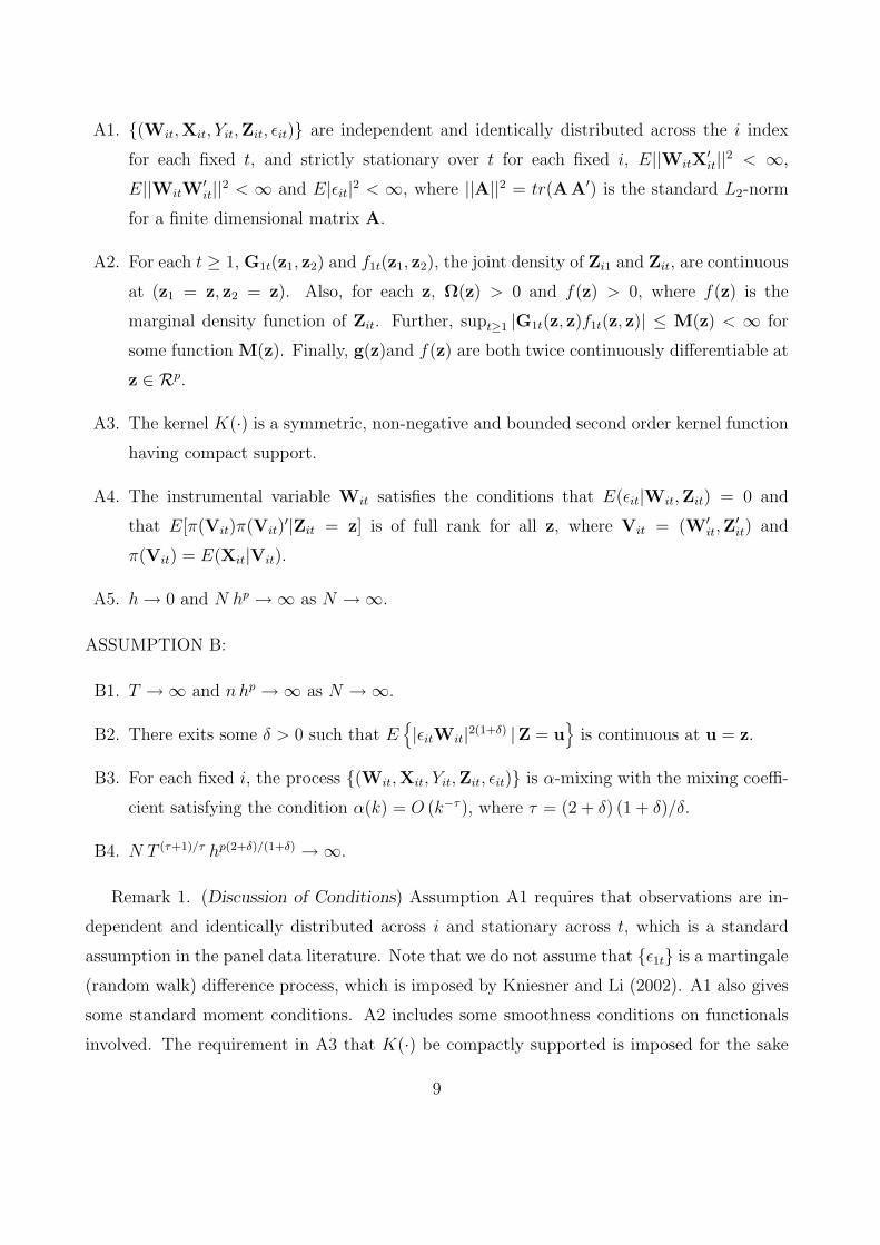
A1. (Wit,Xit, Yit,Zit, ǫit) are independent and identically distributed across the i index

for each fixed t, and strictly stationary over t for each fixed i, E||WitX′it||2 < ∞,

E||WitW′it||2 < ∞ and E|ǫit|2 < ∞, where ||A||2 = tr(AA′) is the standard L2-norm

for a finite dimensional matrix A.

A2. For each t ≥ 1, G1t(z1, z2) and f1t(z1, z2), the joint density of Zi1 and Zit, are continuous

at (z1 = z, z2 = z). Also, for each z, Ω(z) > 0 and f(z) > 0, where f(z) is the

marginal density function of Zit. Further, supt≥1 |G1t(z, z)f1t(z, z)| ≤ M(z) < ∞ for

some function M(z). Finally, g(z)and f(z) are both twice continuously differentiable at

z ∈ Rp.

A3. The kernel K(·) is a symmetric, non-negative and bounded second order kernel function

having compact support.

A4. The instrumental variable Wit satisfies the conditions that E(ǫit|Wit,Zit) = 0 and

that E[π(Vit)π(Vit)′|Zit = z] is of full rank for all z, where Vit = (W′

it,Z′it) and

π(Vit) = E(Xit|Vit).

A5. h → 0 and N hp → ∞ as N → ∞.

ASSUMPTION B:

B1. T → ∞ and nhp → ∞ as N → ∞.

B2. There exits some δ > 0 such that E|ǫitWit|2(1+δ) |Z = u

is continuous at u = z.

B3. For each fixed i, the process (Wit,Xit, Yit,Zit, ǫit) is α-mixing with the mixing coeffi-

cient satisfying the condition α(k) = O (k−τ ), where τ = (2 + δ) (1 + δ)/δ.

B4. N T (τ+1)/τ hp(2+δ)/(1+δ) → ∞.

Remark 1. (Discussion of Conditions) Assumption A1 requires that observations are in-

dependent and identically distributed across i and stationary across t, which is a standard

assumption in the panel data literature. Note that we do not assume that ǫ1t is a martingale

(random walk) difference process, which is imposed by Kniesner and Li (2002). A1 also gives

some standard moment conditions. A2 includes some smoothness conditions on functionals

involved. The requirement in A3 that K(·) be compactly supported is imposed for the sake

9

of brevity of proofs, and can be removed at the cost of lengthier arguments. In particular,

the Gaussian kernel is allowed. A4 is a necessary and sufficient condition for model identi-

fication. A5 allows for T either fixed (bounded) or going to infinity. When T is fixed, the

theoretical results are similar to the cross-sectional data case. But for large T (T → ∞), the

mathematical derivation is more involved. Therefore, for large T , we need some additional

(stronger) conditions such as B2 - B4. In particular, B2 requires the existence of some high

order moments. α-mixing is one of the weakest mixing conditions for weakly dependent sto-

chastic processes. Stationary time series or Markov chains fulfilling certain (mild) conditions

are α-mixing with exponentially decaying coefficients; see Cai (2002) and Carrasco and Chen

(2002) for additional examples. On the other hand, the assumption on the convergence rate of

α(k) in B3 might not be the weakest possible and is imposed to simplify the proof. Conditions

B2 - B4 are similar to those needed for nonlinear time series models (e.g., Cai, Fan and Yao

(2000)). Finally, we note that B4 is not restrictive, for example, if we consider the optimal

bandwidth such that hopt = O(n−1/(p+4)) (see Remark 3 below), then, B4 is satisfied when

δ ≥ p/4 − 1. Therefore, the conditions imposed here are quite mild and standard.

Before presenting some auxiliary results, we need to introduce some notation. Denote

Rj(Zit, z) = gj(Zit) − aj − b′j (Zit − z) − 1

2(Zit − z)′ ∇2gj(z) (Zit − z),

Bn =1

n

N∑

i=1

T∑

t=1

Kh(Zit − z)Qit

1

2

d∑

j=1

(Zit − z)′ ∇2gj(z) (Zit − z) Xitj,

Rn =1

n

N∑

i=1

T∑

t=1

Kh(Zit − z)Qit

d∑

j=1

Rj(Zit, z) Xitj,

and

T∗n =

1

n

N∑

i=1

T∑

t=1

Kh(Zit − z)Qit ǫit.

Then, Tn = Sn Hα + T∗n + Bn + Rn. Substituting this into (9), we obtain

H (α − α) − (S′

nSn)−1 S′

n Bn − (S′

nSn)−1 S′

n Rn = (S′

nSn)−1 S′

n T∗n. (10)

In order to establish the asymptotic distribution of α, we will show that the second term

on the left hand side of (10) contributes to the asymptotic bias, the third term on the left

hand side is negligible in probability, and the term on the right hand side is asymptotically

normal. To this end, we first provide some preliminary results stated below with their proofs

relegated to the appendix.

10

PROPOSITION 1. Under Assumptions A1 - A5, we have

(i) Sn = f(z)S 1 + op(1), (ii) Bn =h2

2f(z)B(z) + op(h

2), and (iii) Rn = op(h2).

PROPOSITION 2. (i) Under Assumptions A1 - A4, and B1, and if T hp → 0, then,

nhp Var(T∗n) → f(z)S∗. (11)

(ii) If T hp ≥ C > 0, and Assumptions A1 - A4, and B1 - B3 are satisfied, then (11) holds

true.

It follows from (10), Proposition 1 and Assumption A3 that

H (α − α) − h2

2

(Bg(z)

0

)

+ op(h2) = f−1(z) (S′S)−1 S′ T∗

n1 + op(1), (12)

where Bg(z) =∫A(u, z) K(u) du = (tr(∇2gj(z)µ2(K)))d×1 is a d× 1 vector. The asymptotic

sampling theory for the NPGMM estimators is established in Theorem 1 for consistency and

in Theorems 2 and 3 for asymptotic normality with detailed proofs relegated to the appendix.

THEOREM 1. (i) If T hp → 0, under Assumptions A1 - A5, we have

H (α − α) − h2

2

(Bg(z)

0

)

= op(h2) + Op

((nhp)−1/2

). (13)

(ii) If T hp ≥ C for some C > 0, and Assumptions A1 - A5, B2 and B3 are satisfied, then

(13) holds true.

The proof of Theorem 1 is straightforward from Proposition 2 and (12) and is therefore

omitted.

Remark 2. Theorem 1 shows that α is consistent (with rate of convergence) for both

large and small T cases. In particular, for the case where T hp → 0, it does not require

any assumptions on the dependence structure such as Assumption B3. This is particularly

useful in practice. For example, it covers models with serially correlated errors. The next two

theorems give the asymptotic normal distribution for α for fixed and large T cases.

THEOREM 2. If T is finite, under Assumptions A1 - A5 and B2, we have

√nhp

[

H (α − α) − h2

2

(Bg(z)

0

)

+ op(h2)

]d→ N

(0, f−1(z)∆

), (14)

11

where ∆ = diagν0Ωg,Ωg ⊗ [µ−12 (K)µ2(K

2)µ−12 (K)] with Ωg = (Ω′Ω)−1Ω′ Ω1 Ω(Ω′Ω)−1.

THEOREM 3. If T → ∞, and Assumptions A1 - A5, and B2 - B4 are satisfied. Then

(14) holds true. In particular we have,

√nhp

[

g(z) − g(z) − h2

2Bg(z) + op(h

2)

]d→ N

(0, ν0 f−1(z)Ωg

).

To prove the asymptotic normality results stated in Theorems 2 and 3, given the results

of Theorem 1, it suffices to show that√

nhp T∗n → N(0, f(z)S∗(z)), which is proved in the

appendix.

Remark 3. From Theorem 2 it is easy to see that the asymptotic variance of√

nhp(g(z)−g(z)) is ν0f

−1(z)Ωg, which is the same as that given in Theorem 3. Hence, Theorems 2 and

3 show that g(z) has the same leading bias and variance expressions for both finite T and

the large T cases. This implies if one first let N → ∞ (for a fixed value of T ), and then let

T → ∞; this sequential limit is the same as the joint limit of N → ∞ and T → ∞. Therefore,

we know that the asymptotic mean squares error (AMSE) of g(z), whether T is fixed or large,

is given by

AMSE = h4||Bg(z)||2/4 + ν0f−1(z) tr(Ωg)(nhp)−1.

Then it is easy to show that the optimal bandwidth hopt that minimizes the above AMSE is

given by

hopt =(p ν0 f−1(z) tr(Ωg) ||Bg(z)||−2

)1/(p+4)n−1/(p+4)

and the resulting optimal AMSE is

AMSEopt =(p4/(p+4)/ + p−p/(p+4)

) (ν0 tr(Ωg)f

−1(z))4/(p+4) ||Bg(z)||2p/(p+4)n−4/(p+4),

which is the optimal rate of convergence.

Also, it can be shown that, when T is sufficiently large and N is small, the results of

Theorem 3 still hold although the theoretical justification needs some modifications.

Finally, let us consider the special case when model (1) does not have any endogenous

variable, (e.g., Wit = Xit). For this case, we have the following asymptotic normality result

for the local linear estimator of the coefficient functions, which covers the results in Cai, Fan

and Yao (2000).

12

THEOREM 4. (i) Under Assumptions A1 - A5 and B2, if T is finite, then we have

√nhp

[

g(z) − g(z) − h2

2Bg(z) + op(h

2)

]

→ N(0, ν0 f−1(z)Ω∗

g(z)), (15)

where

Ω∗g(z) =

[E

Xit X

′it

∣∣∣ Zit = z]−1

Eσ2(Vit) Xit X

′it

∣∣∣ Zit = z [

EXit X

′it

∣∣∣ Zit = z]−1

.

(ii) If T → ∞, and Assumptions A1 - A5, and B2 - B4 are satisfied, then (15) holds true.

Remark 4. Note first that Theorem 4 (i) and (ii) are special cases of Theorems 2 and 3 by

letting Wit = Xit. Also, Remarks 2 and 3 are applicable here for Theorem 4.

Remark 5. It is quite difficult to compare the relative efficiency of our estimator and

two-stage estimator proposed by Cai et al (2006) for the general set up. For the simplest

case that both Xit and Wit are scalars and that the error is conditional homogenous, one

can show that Cai et al’s (2006) two-stage estimator is asymptotically more efficient than

the estimator proposed in this paper (in the sense of having smaller asymptotic variance).

However, since Cai et al’s (2006) estimator requires one first estimates a high dimensional

nonparametric regression model, this will affect the finite sample performance of Cai et al’s

(2006) estimator. If one focuses on the first order condition of (5), then Cai and Li (2005)

showed that the optimal choice of Q(Vit) is Q(Vit) = E(Xit|Vit)/σ2(Vit) and the resulting

estimator will be asymptotically more efficient than both the estimator discussed in section 3

of this paper and the two-stage estimator of Cai et al (2006). However, a general treatment

of efficient estimation is complex because (5) does not take care of the correlation of the T

moment conditions.1 We leave the general efficient estimation problem as a topic for future

research.

REFERENCES

Ai, C. & X. Chen (2003) Efficient estimation of models with conditional moment restrictionsconditioning unknown functions. Econometrica 71, 1795-1843.

Arellano, M. (2003) Panel Data Econometrics. Oxford: Oxford University Press.

Baltagi, B. (2005), Econometric Analysis of Panel Data, 2nd Edition, New York: John Wileyand Sons.

Baltagi, B. & Q. Li (2002) On instrumental variable estimation of semiparametric dynamicpanel data models. Economics Letters 76, 1-9.

1We owe this observation to a referee.

13

Cai, Z. (2002). Regression quantiles for time series data. Econometric Theory 18, 169-192.

Cai, Z. (2003) Nonparametric estimation equations for time series data. Statistics and Prob-ability Letters 62, 379-390.

Cai, Z., M. Das, H. Xiong & X. Wu (2006) Functional-coefficient instrumental variablesmodels. Journal of Econometrics 133, 207-241.

Cai, Z., J. Fan & Q. Yao (2000) Functional-coefficient regression models for nonlinear timeseries. Journal of the American Statistical Association 95, 941-956.

Cai, Z. & Q. Li (2005), Nonparametric estimation of varying coefficient dynamic panel datamodels. Working Paper, Department of Economics, Taxes A&M University.

Cai, Z. & H. Xiong (2006) Efficient estimation of partially varying-coefficient instrumentalvariables models. Working Paper, Department of Mathematics and Statistics, Universityof North Carolina at Charlotte.

Carrasco, M. & X. Chen, (2002) Mixing and moment properties of various GARCH andstochastic volatility models. Econometric Theory 18, 17-39.

Chen, R. & R.S. Tsay (1993) Functional-coefficient autoregressive models. Journal of theAmerican Statistical Association 88, 298-308.

Das, M. (2005) Instrumental variables estimators for nonparametric models with discreteendogenous regressors. Journal of Econometrics 124, 335-361.

Fan, J. & I. Gijbels (1996) Local Polynomial Modeling and Its Applications. London: Chap-man and Hall.

Gonzalez, A., T. Terasvirta & D. Van Dijk (2004) Panel smooth transition regression modeland an application to investment under credit constraints. Working Paper, Departmentof Economic Statistics, Stockholm School of Economics.

Granger, C.L.J. & T. Terasvirta (1993) Modelling Nonlinear Economic Relationships. Ox-ford: Oxford University Press.

Hall, P. & C.C. Heyde (1980) Martingale Limit Theory and its Applications. New York:Academic Press.

Hamilton, J.D. (1994) Time Series Analysis. Princeton: Princeton University Precess.

Hansen, B.E. (1999) Threshold effects in non-dynamic panels: Estimation, testing, and in-ference. Journal of Econometrics 93, 345-368.

Hansen, P.L. (1982) Large sample properties of generalized method of moments estimators.Econometrica 50, 1029-1054.

Hastie, T.J., & R. Tibshirani (1993) Varying-coefficient models (with discussion). Journalof the Royal Statistical Society, Series B 55, 757-796.

Hong, Y. & T.-H. Lee (2003) Inference and forecast of exchange rates via generalized spec-trum and nonlinear time series models. The Review of Economics and Statistics 85,1048-1062.

14

Horowitz, J.L. & M. Markatou (1996) Semiparametric estimation of regression models forpanel data. The Review of Economic Studies 63, 145-168.

Hsiao, C. (2003) Analysis of Panel Data, 2nd Edition. Cambridge: Cambridge UniversityPress.

Ibragimov, I.A. & Yu.V. Linnik (1971) Independent and Stationary Sequences of RandomVariables. Groningen, the Netherlands: Walters-Noordhoff.

Juhl, T. (2005) Functional-coefficient models under unit root behavior. Econometrics Journal8, 197-213.

Kniesner, T.J. & Q. Li (2002) Nonlinearity in dynamic adjustment: Semiparametric estima-tion of panel labor supply. Empirical Economics 27, 131-148.

Li, Q. & C. Hsiao (1998) Testing serial correlation in semiparametric panel data models.Journal of Econometrics 87, 207-237.

Li, Q., C. Huang, D. Li & F. Fu (2002) Semiparametric smooth coefficient model. Journalof Business and Economic Statistics 20, 412-422.

Li, Q. & T. Stengos (1996) Semiparametric estimation of partially linear panel data model.Journal of Econometrics 71, 389-397.

Newey, W.K. (1990) Efficient instrumental variables estimation of nonlinear models. Econo-metrica 58, 809-837.

Pesaran, M.H. & R. Smith (1995) Estimating long-run relationships from dynamic heteroge-neous panels. Journal of Econometrics 68, 79-113.

Robertson, D. & J. Symons (1992) Some strange properties of panel data estimators. Journalof Applied Econometrics 7, 175-189.

Shao, Q. & H. Yu (1996) Weak convergence or weighted empirical processes of dependentsequences. The Annals of Probability 24, 2098-2127.

Volkonskii, V.A. & Yu.A. Rozanov (1959) Some limit theorems for random functions. I.Theory of Probability and Its Applications 4, 178-197.

APPENDIX

Before we prove the main results of the paper, for reference convenience, we first present some

lemmas which will be used in the proofs of Theorems 2 and 3, although they are just stated

here without proof. Indeed, Lemma 1 is the so-called Davydov’s inequality which is Corollary

A2 in Hall and Heyde (1980, p.278), Lemma 2 is Lemma 1.1 of Volkonkii and Rozanov (1959)

and also appears in the books by Ibragimov and Linnik (1971, Remark 17.2.1) and Fan and

Gijbels (1996, Lemma 6.1), and Lemma 3 is a part of Theorem 4.1 of Shao and Yu (1996).

For the detailed proofs, see the aforementioned books and papers.

15

LEMMA 1. Suppose that U and V are random variables which are F t−∞ and F∞

t+τ -

measurable, respectively, and that ||U ||p < ∞, ||V ||q < ∞, where ||U ||p = E[|U |p]1/p

and p, q > 1, p−1 + q−1 < 1. Then,

|E(UV ) − E(U)E(V )| ≤ 8[α(τ)]r ||U ||p ||V ||q,

where r = 1 − p−1 − q−1.

LEMMA 2. Let V1, . . . , VL be α mixing stationary random variables which are F j1i1 , . . .,

F jL

iL-measurable, respectively with 1 ≤ i1 < j1 < i2 · · · < jL, il+1 − jl ≥ τ , and |Vl| ≤ 1 for

l = 1, ..., L. Then, ∣∣∣∣∣E

(L∏

l=1

Vl

)

−L∏

l=1

E(Vl)

∣∣∣∣∣ ≤ 16 (L − 1)α(τ).

LEMMA 3. Let 2 < p < r ≤ ∞, and Vt be an α-mixing process with E(Vt) = 0 and

||Vt||r < ∞. Define Sn =∑n

t=n Vt and assume that α(τ) = O(τ−θ) for some θ > p r/(2(r − p).

Then,

E|Sn|p ≤ K np/2 maxt≤n

||Vt||pr,

where K is a finite positive constant.

We use the same notation introduced in Sections 2 and 3. Throughout this appendix, we

denote by C a generic positive constant, which may take different values at different places.

Proof of Proposition 1. By the stationarity given in Assumption A1, we have

E(Sn) = EQit U

′

it Kh(Zit − z)

= E

(WX′ WX′ ⊗ (Z − z)′/h

XW′ ⊗ (Z − z)/h WX′ ⊗ (Z − z)(Z − z)′/h2

)

Kh(Z − z)

= E

(Ω(Z) Ω(Z) ⊗ (Z − z)′/h

Ω′(Z) ⊗ (Z − z)/h Ω(Z) ⊗ (Z − z)(Z − z)′/h2

)

Kh(Z − z)

=∫ (

Ω(u) Ω(u) ⊗ (u − z)′/hΩ′(u) ⊗ (u − z)/h Ω(u) ⊗ (u − z)(u − z)′/h2

)

Kh(u − z) f(u) du

=∫ (

Ω(z + hu) Ω(z + hu) ⊗ u′

Ω′(z + hu) ⊗ u Ω(z + hu) ⊗ uu′

)

K(u) f(z + hu) du → f(z)S(z)

by Assumptions A2 and A3. To establish the assertion in (i), we now define, for 1 ≤ l ≤ q

and 1 ≤ j ≤ d,

sn,lj =1

n

N∑

i=1

T∑

t=1

Witl Xitj Kh(Zit − z),

16

where Witl is the l-th element of Wit and Xitj is the j-th element of Xit. Then, by the

stationarity given in Assumption A1, we have

nhp Var(sn,lj)

=hp

TVar

(T∑

t=1

Witl Xitj Kh(Zit − z)

)

= hp Var (Wi1l Xi1j Kh(Zi1 − z)) +

2 hp

T

T−1∑

t=1

(T − t)Cov(Wi1l Xi1jKh(Zi1 − z),Wi(t+1)l Xi(t+1)jKh(Zi(t+1) − z)

)

≡ I1 + I2.

By Assumptions A1 and A2, it is easy to see that I1 ≤ C. Next, we consider I2. By Cauchy-

Schwarz inequality, |I2| ≤ C T . Therefore, Var(sn,lm) ≤ C/(N hp) → 0 by Assumption A5, so

that1

n

N∑

i=1

T∑

t=1

Wit X′it Kh(Zit − z) = f(z)Ω(z) + op(1). (A.1)

Similarly, one can show that

1

n

N∑

i=1

T∑

t=1

Wit X′it ⊗

(Zit − z

h

)

Kh(Zit − z) = op(1)

and

1

n

N∑

i=1

T∑

t=1

Wit X′it ⊗

(Zit − z

h

) (Zit − z

h

)′

Kh(Zit − z) = f(z)Ω(z) ⊗ µ2(K) + op(1).

Hence, we have proved (i).

Next, we prove (ii). Indeed, it is easy to see that

h−2E(Bn) =1

2E

(WitX

′it A((Zit − z)/h)

WitX′it A((Zit − z)/h) ⊗ (Zit − z)/h

)

Kh(Zit − z)

=1

2

∫ (Ω(u)A((u − z)/h)

Ω(u)A((u − z)/h) ⊗ (u − z)/h

)

Kh(u − z)f(u)du

=1

2

∫ (Ω(z + hu)A(u)

Ω(z + hu)A(u) ⊗ u

)

K(u)f(z + hu)du → 1

2f(z)B(z).

Similar to (A.1), it is easy to show that any component of the variance of h−2Bn converges to

zero so that (ii) holds true.

Finally, we establish (iii). To this end, it is not difficult to check that

h−2 E(Rn) = h−2 E

(WitX

′it R(Zit, z)

WitX′it R(Zit, z) ⊗ (Zit − z)/h

)

Kh(Zit − z)

17

= h−2∫ (

Ω(u)R(u, z)Ω(u)R(u, z) ⊗ (u − z)/h

)

Kh(u − z)f(u)du

= h−2∫ (

Ω(z + hu)R(z + hu, z)Ω(z + hu)R(z + hu, z) ⊗ u

)

K(u)f(z + hu)du → 0,

since

h−2Rj(z + hu, z) = h−2[gj(z + hu, z) − gj(z) −∇gj(z)

′(hu) − (1/2)h2u′∇2gj(z)u]

= o(1)

for any u and that any component of the variance of h−2Rn converges to zero.2 Therefore,

(iii) is verified. This completes the proof of Proposition 1.

Proof of Proposition 2. Clearly, E(T∗n) = 0 and

nhp Var(T∗n) =

hp

TVar

(T∑

t=1

Qit ǫit Kh(Zit − z)

)

= hp Var (Qi1 ǫi1 Kh(Zi1 − z)) +

2 hp

T

T−1∑

t=1

(T − t)Cov(Qi1 ǫi1Kh(Zi1 − z),Qi(t+1) ǫi(t+1)Kh(Zi(t+1) − z)

)

≡ I3 + I4.

By Assumptions A1 and A2, I3 → f(z)Ω1(z). Clearly,

|I4| ≤ C hpT−1∑

t=1

∣∣∣Cov(Qi1 ǫi1Kh(Zi1 − z),Qi(t+1) ǫi(t+1)Kh(Zi(t+1) − z)

)∣∣∣ . (A.2)

We now show that the right hand side of the above inequality goes to zero. We consider it in

two cases: (I) T hp → 0 and (II) T hp ≥ C > 0.

Case I: For any t ≥ 1, by Assumption A2,

Cov(Qi1 ǫi1Kh(Zi1 − z),Qi(t+1) ǫi(t+1)Kh(Zi(t+1) − z)

)

= EQi1 Q′

i(t+1) σ2(Wi1,Wi(t+1),Zi1,Zi(t+1))Kh(Zi1 − z)Kh(Zi(t+1) − z)

→ f1,t+1(z, z)

(G1,t+1(z, z) 0

0 G1,t+1(z, z) ⊗ µ2(K)

)

.

By Assumption A2, then

|I4| ≤ C hp T → 0. (A.3)

Cases II: First, we split the sum in (A.2) into two parts as I5 =∑dn

t=1(. . .) and I6 =∑

t>dn(· · ·),

where dn is a sequence of positive integers such that dn hp → 0. First, we show that I5 → 0,

2Recall that Rj(Zit, z) = gj(Zit) − aj(z) −∇g(z)′ (Zit − z) − (1/2) (Zit − z)′ ∇2gj(z) (Zit − z).

18

which can be done by an analog of (A.3). Next we consider the upper bound of I6. For this

purpose, we denote by Kνit = Kh(Zit − z) [(Zit − z)/h]ν , where ν = 0 or 1, and use Lemma 1

to obtain

|Cov(ǫi1 Wi1lKν1

i1 , ǫi(t+1) Wi(t+1)mKν2

i(t+1))| ≤ C [α(t)]δ/(2+δ) ||ǫi1 Wi1lKν1

i1 ||2+δ · ||ǫi1 Wi1lKν2

i1 ||2+δ

for ν1, ν2 = 0 or 1. Conditioning on Zi1 and using Assumption B2 yield

E|ǫi1 Wi1lKνi1|2+δ = E

[E

|ǫi1 Wi1l|2+δ

∣∣∣ Zi1

K2+δ

h (Zi1 − z)|Zi1 − z|/hν(2+δ)]

= h−p(1+δ) f(z) E|ǫi1 Wi1l|2+δ

∣∣∣ Zi1 = z ∫

|u|ν(2+δ) K2+δ(u) du

+o(h−p(1+δ))

≤ Ch−p(1+δ) = O(h−p(1+δ)). (A.4)

Then,

|Cov(ǫi1 Wi1lKν1

i1 , ǫi(t+1) Wi(t+1)mKν2

i(t+1))| = O(αδ/(2+δ)(t) h−2p(1+δ)/(2+δ)).

Therefore, the (l, j)-th element of I6 becomes

|I6(l,j)| ≤ C h−pδ/(2+δ)∑

t>dn

[α(t)]δ/(2+δ) = O(h−pδ/(2+δ) d−δn ) → 0

by Assumption B3 and choosing dn such that hp d2n = O(1), so the requirement that dn hp

n → 0

is satisfied. Therefore, I4 → 0. This proves Proposition 2.

To prove Theorems 2 and 3, from (12), clearly, it suffices to establish the asymptotic

normality of√

nhpT∗n. To this end, we now employ the Cramer-Wold device since T∗

n is

multivariate. For any unit vector d ∈ ℜm1 , let ωit = hp/2d′ Qit Kh(Zit − z) ǫit, 1 ≤ i ≤ N and

1 ≤ t ≤ T . Then,√

nhp d′ T∗n =

1√n

N∑

i=1

T∑

t=1

ωit

and by Proposition 2 and (A.2), for any 1 ≤ i ≤ N and 1 ≤ t ≤ T ,

Var(ωit) = f(z)d′ S∗(z)d (1 + o(1)) ≡ θ2(z)(1 + o(1)), andT∑

t=2

|Cov(ωi1, ωit)| = o(1).

Therefore, Var(√

nhp d′ T∗n) = θ2(z)(1 + o(1)).

Proof of Theorem 2. Define ω∗n,i = T−1/2 ∑T

t=1 ωit. Then, ω∗n,i are independent

double array random variables since T is finite and√

nhp d′ T∗n = N−1/2 ∑N

i=1 ω∗n,i. To show

19

the asymptotic normality, it suffices to check the Lyapounov’s condition. By Minkowski’s

inequality and using the similar derivations as those used in the proof of (A.4), we have

E|ω∗n,i|2+δ ≤ C T (2+δ)/2 E|ωi1|2+δ ≤ C T (2+δ)/2 h−pδ/2

by Assumption B2. Therefore, n−(2+δ)/2 ∑Ni=1 E|ω∗

n,i|2+δ ≤ C (N hp)−δ/2 → 0 by Assumption

A5. Thus, we have shown that the Lyapounov’s condition holds and Theorem 2 follows.

Proof of Theorem 3. When T → ∞, for each i, ωi,tTt=1 is a stationary α-mixing

sequence. Therefore, the proof is more complicated; see Hall and Heyde (1980) and Ibragimov

and Linnik (1971). The common approach to prove the asymptotic normality for a station-

ary α-mixing sequence is to employ the Doob’s small-block and large-block technique; see

Ibragimov and Linnik (1971, Chapter 18), Cai (2002, 2003) and Cai, Fan and Yao (2000) for

details. For this setting, we partition 1, . . . , T into 2 qT + 1 subsets with large-block of

size rT and small-block of size sT < T with rT + sT < T and rT and sT specified later. Set

qT = ⌊T/(rT + sT )⌋ and define the random variables, for 0 ≤ j ≤ qT − 1,

ηij =j(rT +sT )+rT∑

t=j(rT +sT )+1

ωit, ξij =(j+1)(rT +sT )∑

t=j(rT +sT )+rT +1

ωit, and ζiqT=

T∑

t=qT (rT +sT )+1

ωit.

Then,

√nhp d′ T∗

n =1√n

N∑

i=1

qT−1∑

j=0

ηij +N∑

i=1

qT−1∑

j=0

ξij +N∑

i=1

ζiqT

≡ 1√nQn,1 + Qn,2 + Qn,3 .

To establish the asymptotic normality of√

nhp d′ T∗n, it suffices to show the followings: as

N → ∞ and T → ∞,

1

nE [Qn,2]

2 → 0,1

nE [Qn,3]

2 → 0, (A.5)

∣∣∣∣∣∣E

exp

i tqT−1∑

j=0

ηkj

−qT−1∏

j=0

E [exp(i t ηkj)]

∣∣∣∣∣∣→ 0, for any 1 ≤ k ≤ N , (A.6)

1

n

N∑

i=1

qT−1∑

j=0

E(η2

ij

)→ θ2(z), (A.7)

and1

n

N∑

i=1

qT−1∑

j=0

E[η2

ijI|ηij| ≥ ǫ θ(z)

√N

]→ 0 (A.8)

20

for every ǫ > 0. The explanations of the above four equations (A.5) - (A.8) are as follows: (A.5)

implies that Qn,2/√

n and Qn,3/√

n are asymptotically negligible in probability; (A.6) shows

that ηkj in Qn,1/√

n are asymptotically independent; and (A.7) and (A.8) are the standard

Lindeberg-Feller conditions for the asymptotic normality of Qn,1/√

n for the independent

setup. It follows from the proof of Theorem 18.4.1 in Ibragimov and Linnik (1971) that

a combination of (A.6) - (A.8) concludes Qn,2/√

n → N(0, θ2(z)). Therefore, since both

Qn,1/√

n and Qn,3/√

n converge to zero in probability, by applying the Slusky’s theorem, we

prove the asymptotic normality of√

nhp d′ T∗n.

The remaining parts of the proof are to verify the above four equations (A.5) - (A.8). First,

let us establish (A.5). For this purpose, we choose the large-block size rT by rT = ⌊T 1/τ⌋ and

the small-block size by sT = ⌊T 1/(τ+1)⌋, where τ is given in Assumption B3 and ⌊x⌋ denotes

the integer part of x. Then, it can easily be shown from Assumption B3 that

sT /rT → 0, rT /T → 0, and qT α(sT ) ≤ C T−1/(τ+1)τ → 0. (A.9)

Observe that

N−1 E [Qn,2]2 =

qT−1∑

j=0

Var(ξij) + 2∑

0≤k<j≤qT−1

Cov(ξik, ξij) ≡ J1 + J2. (A.10)

It follows from the stationarity and Proposition 2 that

J1 = qT Var(ξi1) = qT Var

(sT∑

t=1

ωit

)

= qT sT [θ2(z) + o(1)]. (A.11)

Next consider the second term J2 on the right hand side of (A.10). Let r∗j = j(rT + sT ), then

r∗j − r∗k ≥ rT for all j > k. Therefore, we have

|J2| ≤ 2∑

0≤k<j≤qT−1

sT∑

j1=1

sT∑

j2=1

|Cov(ωi,r∗k+rT +j1 , ωi,r∗

j+rT +j2)| ≤ 2

T−rT∑

j1=1

T∑

j2=j1+rT

|Cov(ωij1 , ωi,j2)|.

By the stationarity and (A.2), one obtains

|J2| ≤ 2TT∑

j=rT +1

|Cov(ωi1, ωij)| = o(T ). (A.12)

Hence, by (A.9)-(A.12), we have

1

nE(Qn,2)

2 = O (qT sT /T ) + o(1) = o(1). (A.13)

21

It follows from the stationarity, (A.9) and Proposition 2 that

Var(Qn,3) = N Var

T−qT (rT +sT )∑

t=1

ωit

= O(N(T − qT (rT + sT ))) = o(n). (A.14)

Combining (A.9), (A.13) and (A.14), we have established (A.5).

To establish (A.6), we use Lemma 2 to obtain

∣∣∣∣∣∣E

exp

i tqT−1∑

j=0

ηkj

−qT−1∏

j=0

E [exp(i t ηkj)]

∣∣∣∣∣∣≤ 16 qT α(sT )

which goes to zero as T → ∞ by (A.9). Therefore, (A.6) is proved.

As for (A.7), by the stationarity, (A.2), (A.9) and Proposition 2, it is easily seen that

1

n

N∑

i=1

qT−1∑

j=0

E(η2

ij

)=

qT

TE

(η2

i1

)=

qT rT

T· 1

rT

Var

(rT∑

t=1

ωit

)

→ θ2(z),

so that (A.7) is proved.

It remains to establish (A.8). For this purpose, we employ Lemma 3 and Assumption B3

to obtain

E[η2

i1 I|ηi1| ≥ ǫ θ(z)

√N

]≤ C N−δ/2 E

(|ηi1|2+δ

)≤ C N−δ/2r

1+δ/2T ||ωi1||2+δ

2+2δ.

Similar to (A.4), one can show easily that

E(|ωi1|2+2δ

)≤ C h−pδ,

which in conjunction with the above result, implies that

E[η2

i1 I|ηi1| ≥ ǫ θ(z)

√n

]≤ C n−δ/2 r

1+δ/2T h−pδ(2+δ)/2(1+δ).

Thus, by the definition of rT , we obtain

1

n

N∑

i=1

qT−1∑

j=0

E[η2

ijI|ηij| ≥ ǫ θ(z)

√n

]≤ C

(N T (τ+1)/τ hp(2+δ)/(1+δ)

)−δ/2

tending to zero by Assumption B4 Thus, this completes the proof of Theorem 3.

22