Embed Size (px)
Citation preview
Nonsmooth and nonconvex optimization under statisticalassumptions
Damek Davis1
School of Operations Research and Information EngineeringCornell University
1https://people.orie.cornell.edu/dsd95/0 / 40
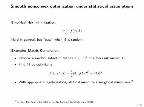
Smooth nonconvex optimization under statistical assumptions
Empirical risk minimization.
minx
f(x;A)
Hard in general, but “easy” when A is random.
Example: Matrix Completion.
• Observe a random subset of entries A ⊆ [n]2 of a low rank matrix M .
• Find M by optimizing
f(L,R;A) = 12‖ΠA(LRT −M)‖2
• With appropriate regularization, all local minimizers are global minimizers.2
2Ge, Lee, Ma. Matrix Completion has No Spurious Local Minimum (2016)1 / 40
Smooth nonconvex optimization under statistical assumptions
Further Examples. Provable complexity guarantees for MatrixCompletion/Sensing, Tensor Recovery/Decomposition and Latent VariableModels, Phase retrieval, Dictionary Learning, Deep Learning,Nonnegative/Sparse Principal Component Analysis, Mixture of LinearRegression, Super Resolution, Synchronization and Community Detection,Joint Alignment Problems, and System Identification.
Extensive list. http://sunju.org/research/nonconvex/
2 / 40
Smooth nonconvex optimization under statistical assumptions
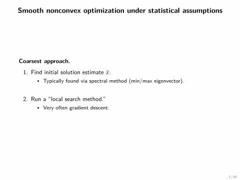
Coarsest approach.
1. Find initial solution estimate x.• Typically found via spectral method (min/max eigenvector).
2. Run a “local search method.”• Very often gradient descent.
3 / 40
Smooth nonconvex optimization under statistical assumptions
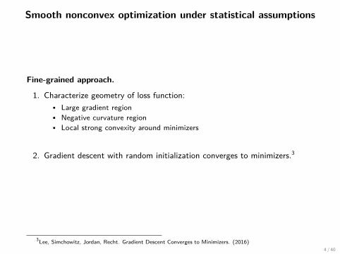
Fine-grained approach.
1. Characterize geometry of loss function:• Large gradient region• Negative curvature region• Local strong convexity around minimizers
2. Gradient descent with random initialization converges to minimizers.3
3Lee, Simchowitz, Jordan, Recht. Gradient Descent Converges to Minimizers. (2016)4 / 40
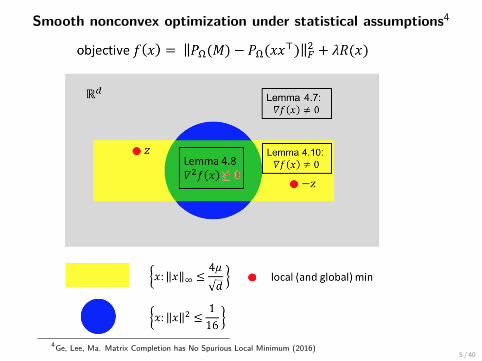
Smooth nonconvex optimization under statistical assumptions4
4Ge, Lee, Ma. Matrix Completion has No Spurious Local Minimum (2016)5 / 40
Smooth nonconvex optimization under statistical assumptions
How to Characterize Geometry.
1. Analyze population riskEA [f(x;A)]
Randomness “integrated out.” Typically simple function.
2. “Transfer” geometry of population model back to empirical risk
f(x;A),
using concentration inequalities.• Gradients and Hessians of empirical risk often concentrate around
population gradients and Hessians.
6 / 40
Smooth nonconvex optimization under statistical assumptions
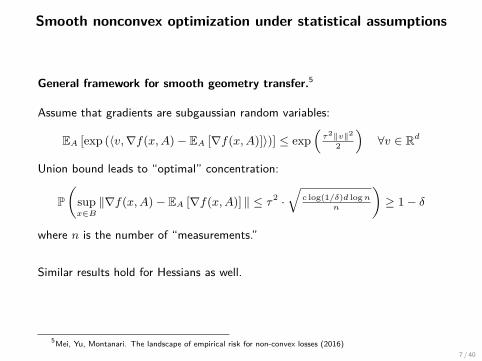
General framework for smooth geometry transfer.5
Assume that gradients are subgaussian random variables:
EA [exp (〈v,∇f(x,A)− EA [∇f(x,A)]〉)] ≤ exp(τ2‖v‖2
2
)∀v ∈ Rd
Union bound leads to “optimal” concentration:
P(
supx∈B‖∇f(x,A)− EA [∇f(x,A)] ‖ ≤ τ2 ·
√c log(1/δ)d logn
n
)≥ 1− δ
where n is the number of “measurements.”
Similar results hold for Hessians as well.
5Mei, Yu, Montanari. The landscape of empirical risk for non-convex losses (2016)7 / 40
Smooth nonconvex optimization under statistical assumptions
Conclusions.
• The pipeline is well-understood.
• Techniques typically tailored to individual problems.
8 / 40

What to do in the nonsmooth setting?
Why should we care?
1. `1-type losses insensitive to outliers/enforce sparsity.
2. ReLU (max0, x) nonsmooth activation units in deep networks verysuccessful in practice.
3. Even in traditional nonlinear programming, difficult constraints c(x) = 0,typically enforced with exact penalty:
‖c(x)‖.
9 / 40
Nonsmooth nonconvex optimization under statistical assumptions
What fails for nonsmooth?
1. Unclear what “local-search” should mean.
2. Geometry• No good quantifiable concept of saddle points (negative eigenvalue of
Hessian).
• Strong convexity 6=⇒ fast convergence.
• Subdifferentials do not concentrate.
What’s coming. Develop general principles for nonsmooth setting, guided byconcrete application.
10 / 40
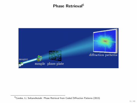
Phase Retrieval6
6Candes, Li, Soltanolkotabi. Phase Retrieval from Coded Diffraction Patterns (2013)11 / 40
Example: nonsmooth phase retrieval
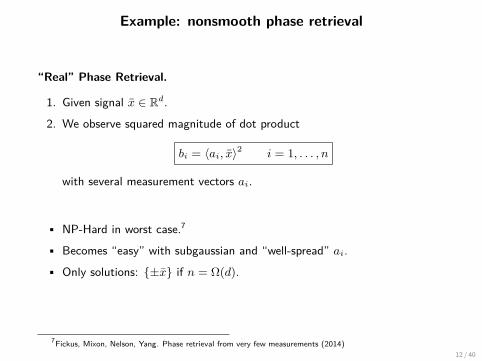
“Real” Phase Retrieval.
1. Given signal x ∈ Rd.
2. We observe squared magnitude of dot product
bi = 〈ai, x〉2 i = 1, . . . , n
with several measurement vectors ai.
• NP-Hard in worst case.7
• Becomes “easy” with subgaussian and “well-spread” ai.
• Only solutions: ±x if n = Ω(d).
7Fickus, Mixon, Nelson, Yang. Phase retrieval from very few measurements (2014)12 / 40
Example: nonsmooth phase retrieval
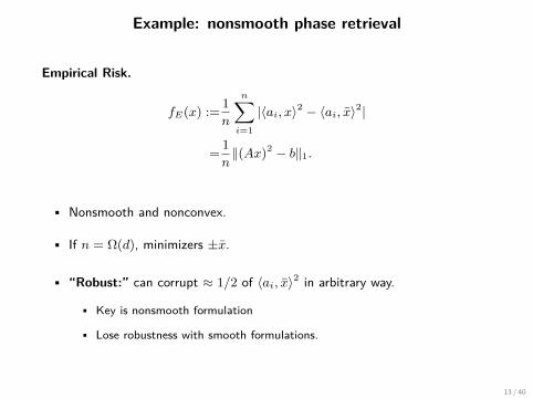
Empirical Risk.
fE(x) := 1n
n∑i=1
|〈ai, x〉2 − 〈ai, x〉2|
= 1n‖(Ax)2 − b‖1.
• Nonsmooth and nonconvex.
• If n = Ω(d), minimizers ±x.
• “Robust:” can corrupt ≈ 1/2 of 〈ai, x〉2 in arbitrary way.
• Key is nonsmooth formulation
• Lose robustness with smooth formulations.
13 / 40
Example: nonsmooth phase retrieval
Key Questions.
1. Linearly convergent algorithm?
2. Stationary point structure?
14 / 40
Linearly convergent algorithm for nonsmooth nonconvex?
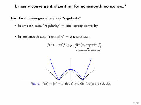
Fast local convergence requires “regularity.”
• In smooth case, “regularity” = local strong convexity.
• In nonsmooth case “regularity” = µ-sharpness:
f(x)− inf f ≥ µ · dist(x, arg min f)︸ ︷︷ ︸distance to solution set
Figure: f(x) = |x2 − 1| (blue) and dist(x; ±1) (black).
15 / 40
Sharpness of fE
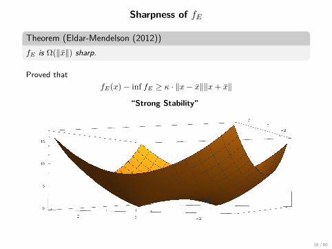
Theorem (Eldar-Mendelson (2012))fE is Ω(‖x‖) sharp.
Proved thatfE(x)− inf fE ≥ κ · ‖x− x‖‖x+ x‖
“Strong Stability”
16 / 40
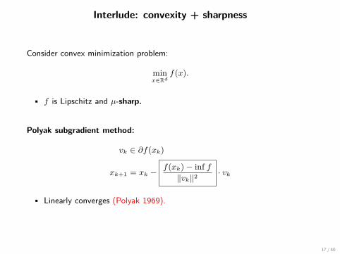
Interlude: convexity + sharpness
Consider convex minimization problem:
minx∈Rd
f(x).
• f is Lipschitz and µ-sharp.
Polyak subgradient method:
vk ∈ ∂f(xk)
xk+1 = xk −f(xk)− inf f‖vk‖2 · vk
• Linearly converges (Polyak 1969).
17 / 40
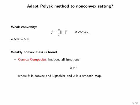
Adapt Polyak method to nonconvex setting?
Weak convexity:f + ρ
2‖ · ‖2 is convex,
where ρ > 0.
Weakly convex class is broad.
• Convex Composite: Includes all functions
h c
where h is convex and Lipschitz and c is a smooth map.
18 / 40
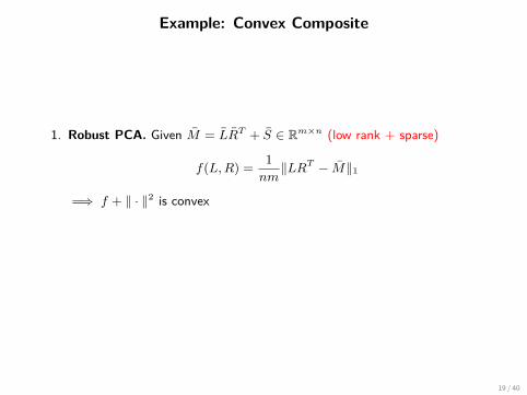
Example: Convex Composite
1. Robust PCA. Given M = LRT + S ∈ Rm×n (low rank + sparse)
f(L,R) = 1nm‖LRT − M‖1
=⇒ f + ‖ · ‖2 is convex
2. Phase Retrieval. fE + 5‖ · ‖2 is convex (w.h.p if ai ∼ N(0, Id))
19 / 40
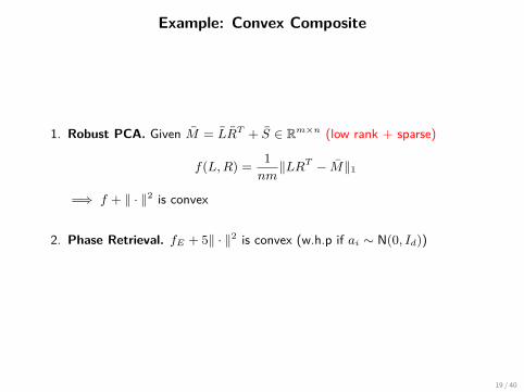
Example: Convex Composite
1. Robust PCA. Given M = LRT + S ∈ Rm×n (low rank + sparse)
f(L,R) = 1nm‖LRT − M‖1
=⇒ f + ‖ · ‖2 is convex
2. Phase Retrieval. fE + 5‖ · ‖2 is convex (w.h.p if ai ∼ N(0, Id))
19 / 40
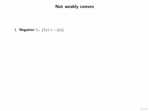
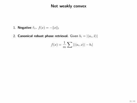
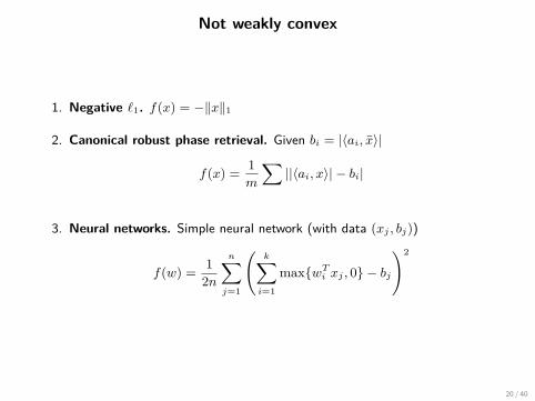
Not weakly convex
1. Negative `1. f(x) = −‖x‖1
2. Canonical robust phase retrieval. Given bi = |〈ai, x〉|
f(x) = 1m
∑||〈ai, x〉| − bi|
3. Neural networks. Simple neural network (with data (xj , bj))
f(w) = 12n
n∑j=1
(k∑i=1
maxwTi xj , 0 − bj
)2
20 / 40
Not weakly convex
1. Negative `1. f(x) = −‖x‖1
2. Canonical robust phase retrieval. Given bi = |〈ai, x〉|
f(x) = 1m
∑||〈ai, x〉| − bi|
3. Neural networks. Simple neural network (with data (xj , bj))
f(w) = 12n
n∑j=1
(k∑i=1
maxwTi xj , 0 − bj
)2
20 / 40
Not weakly convex
1. Negative `1. f(x) = −‖x‖1
2. Canonical robust phase retrieval. Given bi = |〈ai, x〉|
f(x) = 1m
∑||〈ai, x〉| − bi|
3. Neural networks. Simple neural network (with data (xj , bj))
f(w) = 12n
n∑j=1
(k∑i=1
maxwTi xj , 0 − bj
)2
20 / 40
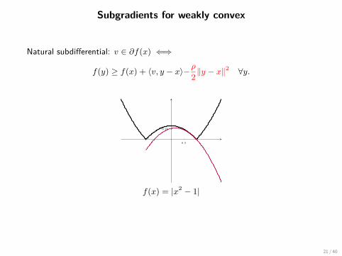
Subgradients for weakly convex
Natural subdifferential: v ∈ ∂f(x) ⇐⇒
f(y) ≥ f(x) + 〈v, y − x〉−ρ2‖y − x‖2 ∀y.
0.5
0.75
f(x) = |x2 − 1|
21 / 40
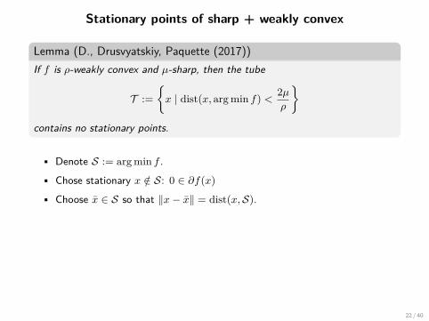
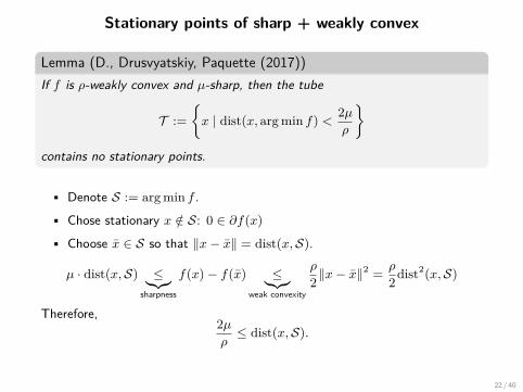
Stationary points of sharp + weakly convex
Lemma (D., Drusvyatskiy, Paquette (2017))If f is ρ-weakly convex and µ-sharp, then the tube
T :=x | dist(x, arg min f) < 2µ
ρ
contains no stationary points.
• Denote S := arg min f .
• Chose stationary x /∈ S: 0 ∈ ∂f(x)
• Choose x ∈ S so that ‖x− x‖ = dist(x,S).
µ · dist(x,S) ≤︸︷︷︸sharpness
f(x)− f(x) ≤︸︷︷︸weak convexity
ρ
2‖x− x‖2 = ρ
2dist2(x,S)
Therefore,2µρ≤ dist(x,S).
22 / 40
Polyak for sharp + weakly convex
Theorem (D., Drusyatskiy, Paquette (2017))Polyak method linearly converges when initialized in T .
• Follow up work for case when inf f is not known.8
• Little was known about convergence rates of subgradient methods fornonconvex problems until quite recently.9 10
• Other problems• Covariance estimation, blind deconvolution, robust PCA, matrix
completion....11
8D., Drusvyatskiy, MacPhee, Paquette (2018)9D., Grimmer. Proximally guided stochastic subgradient method for nonsmooth, nonconvex problems (2017)
10D., Drusvyatskiy. Stochastic model-based minimization of weakly convex functions. (2018)11Charisopoulos, Chen, D., Diaz, Ding, Drusvyatskiy. Low-rank matrix recovery with composite optimization:
good conditioning and rapid convergence. (2019)23 / 40
Consequences for phase retrieval
Theorem (D., Drusvyatskiy, Paquette (2017))Suppose n = Ω(d). After spectral initialization, the Polyak method convergeslinearly on fE .
• In phase retrieval, µ = Ω(‖x‖), ρ = O(1)
T =x | dist(x, ±x)
‖x‖ = O(1).
• Spectral initialization can produce initializer in T .12
• Cost per iteration is two matrix multiplications
2n
n∑i=1
〈ai, x〉sign(〈ai, x〉2 − 〈ai, x〉2)ai ∈ ∂fE(x).
12Duchi, Ruan. Solving (most) of a set of quadratic equalities: Composite optimization for robust phaseretrieval. (2017)
24 / 40
Polyak for sharp + weakly convex: experiment
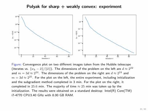
Figure: Convergence plot on two different images taken from the Hubble telescope(iterates vs. ‖xk − x‖/‖x‖). The dimensions of the problem on the left are d ≈ 222
and m = 3d ≈ 224. The dimensions of the problem on the right are d ≈ 224 andm = 3d ≈ 225. For the plot on the left, the entire experiment, including initializationand the subgradient method completed in 3 min. For the plot on the right, itcompleted in 25.6 min. The majority of time ≈ 25 min was taken up by theinitialization. The results were obtained on a standard desktop: Intel(R) Core(TM)i7-4770 CPU3.40 GHz with 8.00 GB RAM.
25 / 40
Comparison to smooth case
fS(x) = 1n
n∑i=1
|〈ai, x〉2 − 〈ai, x〉2|2
• Poorly conditioned near ±x:
12I ∇
2fS(x) O(d)I.
• Overly pessimistic contraction factor:
‖xk+1 − x‖ ≤ (1−O(1/d))‖xk − x‖.
To overcome, carefully analyze trajectory of gradient descent.13
• Nonsmooth Polyak fast “out-of-the-box:” constant contraction factor.
13Chi, Lu, and Chen. Nonconvex Optimization Meets Low-Rank Matrix Factorization: An Overview (2019)26 / 40
Example: nonsmooth phase retrieval
Key Questions.
1. Linearly convergent algorithm?
2. Stationary point structure?
27 / 40
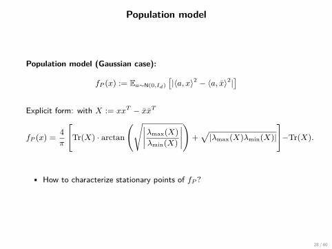
Population model
Population model (Gaussian case):
fP (x) := Ea∼N(0,Id)[|〈a, x〉2 − 〈a, x〉2|
]Explicit form: with X := xxT − xxT
fP (x) = 4π
[Tr(X) · arctan
(√∣∣∣∣λmax(X)λmin(X)
∣∣∣∣)
+√|λmax(X)λmin(X)|
]−Tr(X).
• How to characterize stationary points of fP ?
28 / 40

Spectral function characterization
Lemma (D., Drusvyatskiy, Paquette (2017))There is a symmetric convex function gP satisfying
fP (x) = gP (λ(X)).
where λ(X) is the vector of eigenvalues of X := xxT − xxT .
• Still nonconvex and nonsmooth.
• Exploit symmetries to characterize stationary points.
• Instead of thinking about fP , analyze all functions of the same form.
29 / 40
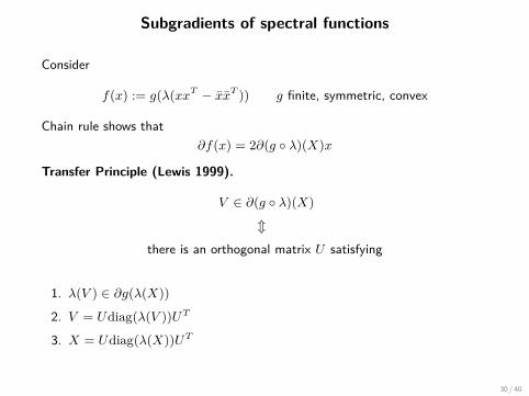
Subgradients of spectral functions
Consider
f(x) := g(λ(xxT − xxT )) g finite, symmetric, convex
Chain rule shows that∂f(x) = 2∂(g λ)(X)x
Transfer Principle (Lewis 1999).
V ∈ ∂(g λ)(X)
m
there is an orthogonal matrix U satisfying
1. λ(V ) ∈ ∂g(λ(X))
2. V = Udiag(λ(V ))UT
3. X = Udiag(λ(X))UT
30 / 40
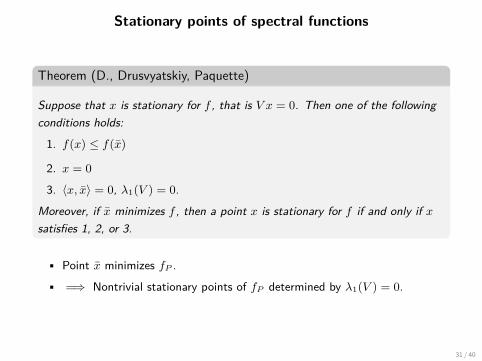
Stationary points of spectral functions
Theorem (D., Drusvyatskiy, Paquette)
Suppose that x is stationary for f , that is V x = 0. Then one of the followingconditions holds:
1. f(x) ≤ f(x)
2. x = 0
3. 〈x, x〉 = 0, λ1(V ) = 0.
Moreover, if x minimizes f , then a point x is stationary for f if and only if xsatisfies 1, 2, or 3.
• Point x minimizes fP .
• =⇒ Nontrivial stationary points of fP determined by λ1(V ) = 0.
31 / 40
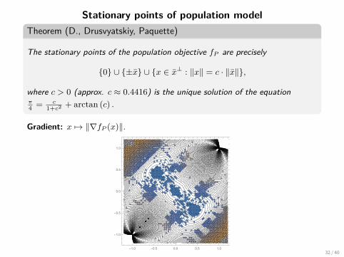
Stationary points of population modelTheorem (D., Drusvyatskiy, Paquette)
The stationary points of the population objective fP are precisely
0 ∪ ±x ∪ x ∈ x⊥ : ‖x‖ = c · ‖x‖,
where c > 0 (approx. c ≈ 0.4416) is the unique solution of the equationπ4 = c
1+c2 + arctan (c) .
Gradient: x 7→ ‖∇fP (x)‖.
-1.0 -0.5 0.0 0.5 1.0
-1.0
-0.5
0.0
0.5
1.0
32 / 40
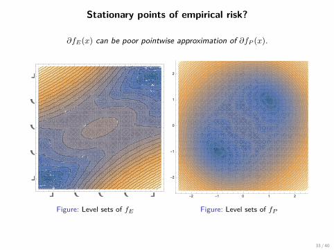
Stationary points of empirical risk?
∂fE(x) can be poor pointwise approximation of ∂fP (x).
1.00.50.00.51.01.00.50.00.51.0
Figure: Level sets of fE Figure: Level sets of fP
33 / 40
Function value concentration
Theorem (Eldar-Mendelson (2012))With high probability
|fE(x)− fP (x)| ≤ C ·√d
n‖x− x‖‖x+ x‖ for all x ∈ Rd.
Does function value approximation imply any “closeness” ofsubdifferentials?
• Hausdorff distance plays key role.
34 / 40
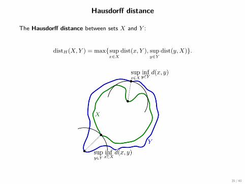
Hausdorff distance
The Hausdorff distance between sets X and Y :
distH(X,Y ) = maxsupx∈X
dist(x, Y ), supy∈Y
dist(y,X).
35 / 40
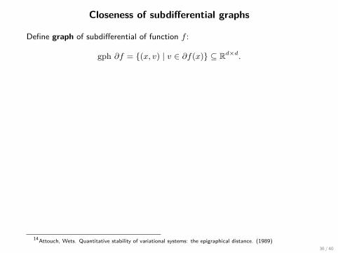
Closeness of subdifferential graphs
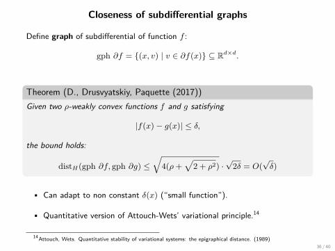
Define graph of subdifferential of function f :
gph ∂f = (x, v) | v ∈ ∂f(x) ⊆ Rd×d.
Theorem (D., Drusvyatskiy, Paquette (2017))Given two ρ-weakly convex functions f and g satisfying
|f(x)− g(x)| ≤ δ,
the bound holds:
distH(gph ∂f, gph ∂g) ≤√
4(ρ+√
2 + ρ2) ·√
2δ = O(√δ)
• Can adapt to non constant δ(x) (“small function”).
• Quantitative version of Attouch-Wets’ variational principle.14
14Attouch, Wets. Quantitative stability of variational systems: the epigraphical distance. (1989)36 / 40
Closeness of subdifferential graphs
Define graph of subdifferential of function f :
gph ∂f = (x, v) | v ∈ ∂f(x) ⊆ Rd×d.
Theorem (D., Drusvyatskiy, Paquette (2017))Given two ρ-weakly convex functions f and g satisfying
|f(x)− g(x)| ≤ δ,
the bound holds:
distH(gph ∂f, gph ∂g) ≤√
4(ρ+√
2 + ρ2) ·√
2δ = O(√δ)
• Can adapt to non constant δ(x) (“small function”).
• Quantitative version of Attouch-Wets’ variational principle.14
14Attouch, Wets. Quantitative stability of variational systems: the epigraphical distance. (1989)36 / 40
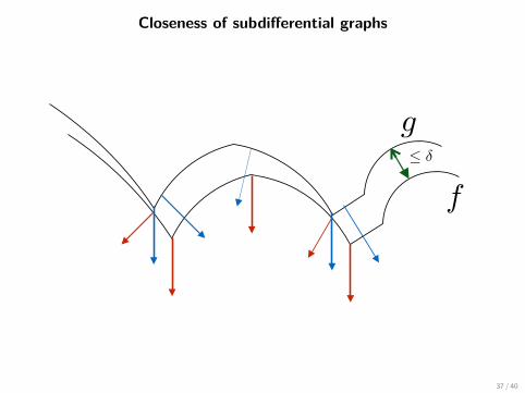
Closeness of subdifferential graphs
g
f
37 / 40
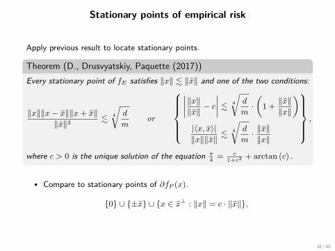
Stationary points of empirical risk
Apply previous result to locate stationary points.
Theorem (D., Drusvyatskiy, Paquette (2017))Every stationary point of fE satisfies ‖x‖ . ‖x‖ and one of the two conditions:
‖x‖‖x− x‖‖x+ x‖‖x‖3 . 4
√d
mor
∣∣∣∣‖x‖‖x‖ − c
∣∣∣∣ . 4
√d
m·(
1 + ‖x‖‖x‖
)|〈x, x〉|‖x‖‖x‖ . 4
√d
m· ‖x‖‖x‖
,
where c > 0 is the unique solution of the equation π4 = c
1+c2 + arctan (c) .
• Compare to stationary points of ∂fP (x).
0 ∪ ±x ∪ x ∈ x⊥ : ‖x‖ = c · ‖x‖,
38 / 40
Extensions of ideas
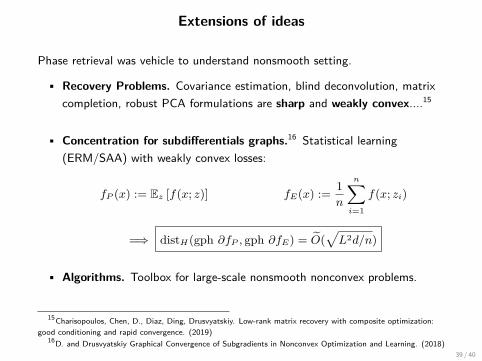
Phase retrieval was vehicle to understand nonsmooth setting.
• Recovery Problems. Covariance estimation, blind deconvolution, matrixcompletion, robust PCA formulations are sharp and weakly convex....15
• Concentration for subdifferentials graphs.16 Statistical learning(ERM/SAA) with weakly convex losses:
fP (x) := Ez [f(x; z)] fE(x) := 1n
n∑i=1
f(x; zi)
=⇒ distH(gph ∂fP , gph ∂fE) = O(√L2d/n)
• Algorithms. Toolbox for large-scale nonsmooth nonconvex problems.
15Charisopoulos, Chen, D., Diaz, Ding, Drusvyatskiy. Low-rank matrix recovery with composite optimization:good conditioning and rapid convergence. (2019)
16D. and Drusvyatskiy Graphical Convergence of Subgradients in Nonconvex Optimization and Learning. (2018)39 / 40
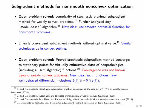
Subgradient methods for nonsmooth nonconvex optimization
• Open problem solved: complexity of stochastic proximal subgradientmethod for weakly convex problems.17 Further analyzed any“model-based” algorithm.18 New idea: use smooth potential function fornonsmooth problems.
• Linearly convergent subgradient methods without optimal value.19 Similartechniques as in convex setting.
• Open problem solved: Proved stochastic subgradient method convergesto stationary points for virtually exhaustive class of nonpathological(including all semialgebraic) functions.20 Convergence was not knownbeyond weakly convex problems. New idea: such functions havewell-behaved differential inclusions z(t) ∈ −∂f(z(t)).
17D. and Drusvyatskiy. Stochastic subgradient method converges at the rate O(k−1/4) on weakly convexfunctions (2018)
18D. and Drusvyatskiy. Stochastic model-based minimization of weakly convex functions (2018)19D. and Drusvyatskiy, MacPhee, and Paquette. Subgradient methods for sharp weakly convex functions (2018)20D., Drusvyatskiy, Kakade, Lee. Stochastic subgradient method converges on tame functions (2018)
40 / 40
Thanks!
• The nonsmooth landscape of phase retrieval. (2017)D., Drusvyatskiy, Paquette. IMA Journal of Numerical Analysis
• Subgradient methods for sharp weakly convex functions. (2018)D., Drusvyatskiy, MacPhee, Paquette. JOTA
• Stochastic model-based minimization of weakly convex functions. (2018)D., Drusvyatskiy. SIOPT
• Stochastic subgradient method converges on tame functions. (2018)D., Drusvyatskiy, Kakade, Lee. FOCM
• Graphical Convergence of Subgradients in Nonconvex Optimization andLearning. (2018)D., Drusvyatskiy, Kakade, Lee. arXiv:1810.07590
• Composite optimization for robust blind deconvolution. (2019)Charisopoulos, D., Dıaz, Drusvyatskiy. arXiv:1901.01624
• Low-rank matrix recovery with composite optimization: good conditioningand rapid convergence. (2019)Charisopoulos, Chen, D., Ding, Dıaz, Drusvyatskiy. arXiv:1904.10020
40 / 40