Embed Size (px)
Citation preview
Front. Math. China 2014, 9(1): 93–99DOI 10.1007/s11464-013-0349-z
Normal projection:deterministic and probabilistic algorithms
Dongmei LI1, Jinwang LIU1, Weijun LIU2
1 Department of Mathematics and Computing Sciences, Hunan University of Scienceand Technology, Xiangtan 411201, China
2 Department of Mathematics and Statistics, Central South University, Changsha 410083,China
c© Higher Education Press and Springer-Verlag Berlin Heidelberg 2013
Abstract We consider the following problem: for a collection of points in ann-dimensional space, find a linear projection mapping the points to the groundfield such that different points are mapped to different values. Such projectionsare called normal and are useful for making algebraic varieties into normalpositions. The points may be given explicitly or implicitly and the coefficientsof the projection come from a subset S of the ground field. If the subset Sis small, this problem may be hard. This paper deals with relatively large S,a deterministic algorithm is given when the points are given explicitly, and alower bound for success probability is given for a probabilistic algorithm fromin the literature.
Keywords Normal projection, primary decomposition of ideal, deterministicalgorithmMSC 13B25, 13F20, 16D25
1 Introduction
In several applications, one often encounters the following problem: for acollection of m different points p1, . . . , pm ∈ kn, where k is an arbitrary field,and a subset S ⊆ k, find c ∈ Sn such that the inner products (c, p1), . . . , (c, pm)are distinct in k. The points pi’s may be given explicitly or implicitly inapplications [10–12,16–18]. For example, in algebraic geometry, suppose thatI is a zero-dimensional ideal in the polynomial ring k[x1, . . . , xn]. The pointspi’s are the zeros of I over the algebraic closure of k. To make I into Noethernormal position, one needs to find
Received July 18, 2013; accepted December 4, 2013Corresponding author: Weijun LIU, E-mail: [email protected]
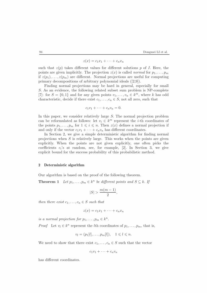
94 Dongmei LI et al.
z(x) = c1x1 + · · · + cnxn
such that z(p) takes different values for different solutions p of I. Here, thepoints are given implicitly. The projection z(x) is called normal for p1, . . . , pm
if z(p1), . . . , z(pm) are different. Normal projections are useful for computingprimary decompositions of arbitrary polynomial ideals ([2,9]).
Finding normal projections may be hard in general, especially for smallS. As an evidence, the following related subset sum problem is NP-complete[7]: for S = {0, 1} and for any given points v1, . . . , vn ∈ km, where k has oddcharacteristic, decide if there exist c1, . . . , cn ∈ S, not all zero, such that
c1v1 + · · · + cnvn = 0.
In this paper, we consider relatively large S. The normal projection problemcan be reformulated as follows: let vi ∈ km represent the i-th coordinates ofthe points p1, . . . , pm for 1 � i � n. Then z(x) defines a normal projection ifand only if the vector c1v1 + · · · + cnvn has different coordinates.
In Section 2, we give a simple deterministic algorithm for finding normalprojections when S is relatively large. This works when the points are givenexplicitly. When the points are not given explicitly, one often picks thecoefficients ci’s at random, see, for example, [2]. In Section 3, we giveexplicit bound for the success probability of this probabilistic method.
2 Deterministic algorithm
Our algorithm is based on the proof of the following theorem.
Theorem 1 Let p1, . . . , pm ∈ kn be different points and S ⊆ k. If
|S| >m(m − 1)
2,
then there exist c1, . . . , cn ∈ S such that
z(x) = c1x1 + · · · + cnxn
is a normal projection for p1, . . . , pm ∈ kn.
Proof Let vl ∈ kn represent the lth coordinates of p1, . . . , pm, that is,
vl = (p1[l], . . . , pm[l]), 1 � l � n.
We need to show that there exist c1, . . . , cn ∈ S such that the vector
c1v1 + · · · + cnvn
has different coordinates.
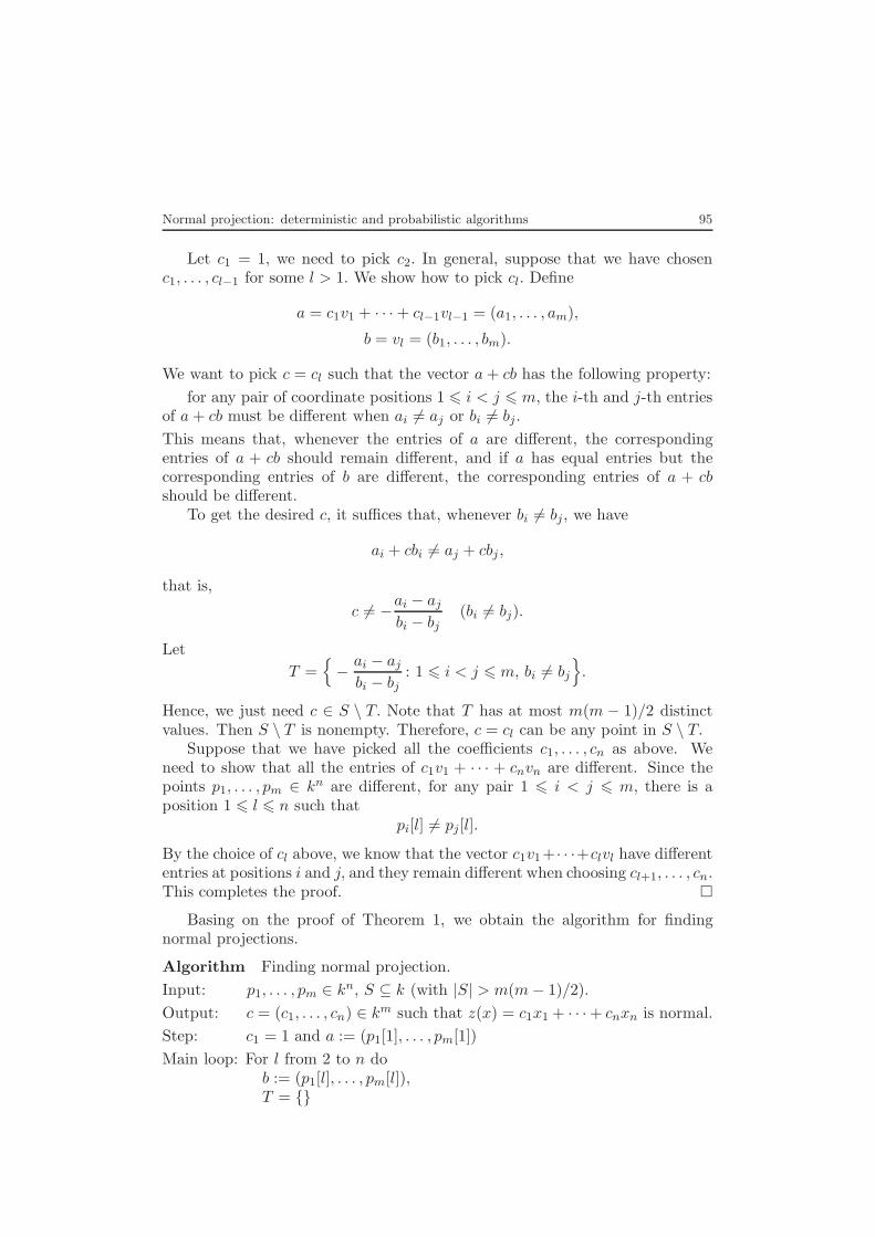
Normal projection: deterministic and probabilistic algorithms 95
Let c1 = 1, we need to pick c2. In general, suppose that we have chosenc1, . . . , cl−1 for some l > 1. We show how to pick cl. Define
a = c1v1 + · · · + cl−1vl−1 = (a1, . . . , am),
b = vl = (b1, . . . , bm).
We want to pick c = cl such that the vector a + cb has the following property:for any pair of coordinate positions 1 � i < j � m, the i-th and j-th entries
of a + cb must be different when ai �= aj or bi �= bj.
This means that, whenever the entries of a are different, the correspondingentries of a + cb should remain different, and if a has equal entries but thecorresponding entries of b are different, the corresponding entries of a + cbshould be different.
To get the desired c, it suffices that, whenever bi �= bj, we have
ai + cbi �= aj + cbj ,
that is,
c �= −ai − aj
bi − bj(bi �= bj).
LetT =
{− ai − aj
bi − bj: 1 � i < j � m, bi �= bj
}.
Hence, we just need c ∈ S \ T. Note that T has at most m(m − 1)/2 distinctvalues. Then S \ T is nonempty. Therefore, c = cl can be any point in S \ T.
Suppose that we have picked all the coefficients c1, . . . , cn as above. Weneed to show that all the entries of c1v1 + · · · + cnvn are different. Since thepoints p1, . . . , pm ∈ kn are different, for any pair 1 � i < j � m, there is aposition 1 � l � n such that
pi[l] �= pj[l].
By the choice of cl above, we know that the vector c1v1+ · · ·+clvl have differententries at positions i and j, and they remain different when choosing cl+1, . . . , cn.This completes the proof. �
Basing on the proof of Theorem 1, we obtain the algorithm for findingnormal projections.
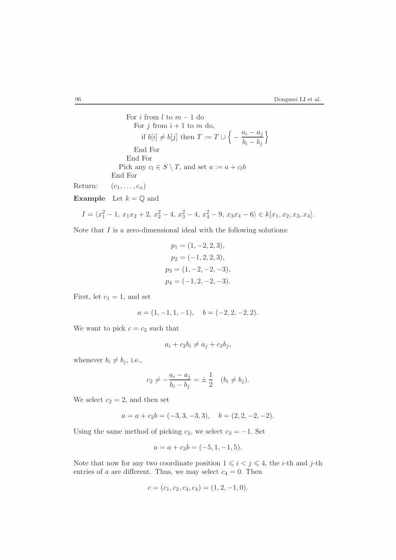
Algorithm Finding normal projection.Input: p1, . . . , pm ∈ kn, S ⊆ k (with |S| > m(m − 1)/2).Output: c = (c1, . . . , cn) ∈ km such that z(x) = c1x1 + · · ·+ cnxn is normal.Step: c1 = 1 and a := (p1[1], . . . , pm[1])Main loop: For l from 2 to n do
b := (p1[l], . . . , pm[l]),T = {}
96 Dongmei LI et al.
For i from l to m − 1 doFor j from i + 1 to m do,
if b[i] �= b[j] then T := T ∪{− ai − aj
bi − bj
}
End ForEnd For
Pick any cl ∈ S \ T, and set a := a + clbEnd For
Return: (c1, . . . , cn)
Example Let k = Q and
I = 〈x21 − 1, x1x2 + 2, x2
2 − 4, x23 − 4, x2
4 − 9, x3x4 − 6〉 ∈ k[x1, x2, x3, x4].
Note that I is a zero-dimensional ideal with the following solutions:
p1 = (1,−2, 2, 3),
p2 = (−1, 2, 2, 3),
p3 = (1,−2,−2,−3),
p4 = (−1, 2,−2,−3).
First, let c1 = 1, and set
a = (1,−1, 1,−1), b = (−2, 2,−2, 2).
We want to pick c = c2 such that
ai + c2bi �= aj + c2bj ,
whenever bi �= bj, i.e.,
c2 �= −ai − aj
bi − bj= ± 1
2(bi �= bj).
We select c2 = 2, and then set
a = a + c2b = (−3, 3,−3, 3), b = (2, 2,−2,−2).
Using the same method of picking c2, we select c3 = −1. Set
a = a + c3b = (−5, 1,−1, 5).
Note that now for any two coordinate position 1 � i < j � 4, the i-th and j-thentries of a are different. Thus, we may select c4 = 0. Then
c = (c1, c2, c3, c4) = (1, 2,−1, 0).

Normal projection: deterministic and probabilistic algorithms 97
3 Success probability for probabilistic method
In computational algebraic geometry, one is often given a zero-dimensionalideal I ⊂ k[x1, . . . , xn] and wants to compute the set of solutions V (I) of Iover the algebraic closure of k or the primary decomposition of I. For primarydecomposition of ideals, we refer to [1–4,6,8,9,13,14]. Here, the set V (I) isunknown, but it is desirable to find a linear function
z(x) = c1x1 + · · · + cnxn
such that z(x) is normal with respect to V (I). In this case, we say that Z(x)is normal for I. The above algorithm cannot be used, since one does not knowthe points explicitly. In practice, one picks the coefficients ci’s from a set Srandomly and independently (see [2,6]). The question is how likely z(x) isnormal for I. The following theorem gives an explicit bound on the successprobability.
Theorem 2 Let I be a zero-dimensional ideal in k[x1, . . . , xn] with degree d,and let S be any subset of k. Pick c1, . . . , cn from S uniform randomly andindependently. Then the probability that z(x) is normal for I is at least
1 − d(d − 1)2|S| .
Proof There are two ways to prove this theorem. The first method is to use[5, Lemma 2.9] in terms of matrix. More precisely, let p1, . . . , pm ∈ kn be allthe distinct solutions in of I. We know that m � d. View each point pi as acolumn vector. Then we get an n × m matrix:
A = (p1, . . . , pm),
where the columns are different. By [5, Lemma 2.9], for random ci ∈ S, theprobability that the vector (c1, . . . , cn)A has different entries is at least
1 − m(m − 1)2|S| � 1 − d(d − 1)
2|S| ,
and hence, the theorem is proved.The other method is to use the well-known Schwartz-Zippel lemma [15,19],
which says that, for any nonzero polynomial
f(y1, . . . , yn) ∈ R[y1, . . . , yn]
of total degree t, where R is an integral domain, and any set S ⊆ R, whenai ∈ S is random and independent for 1 � i � n, the probability that
f(a1, . . . , an) �= 0
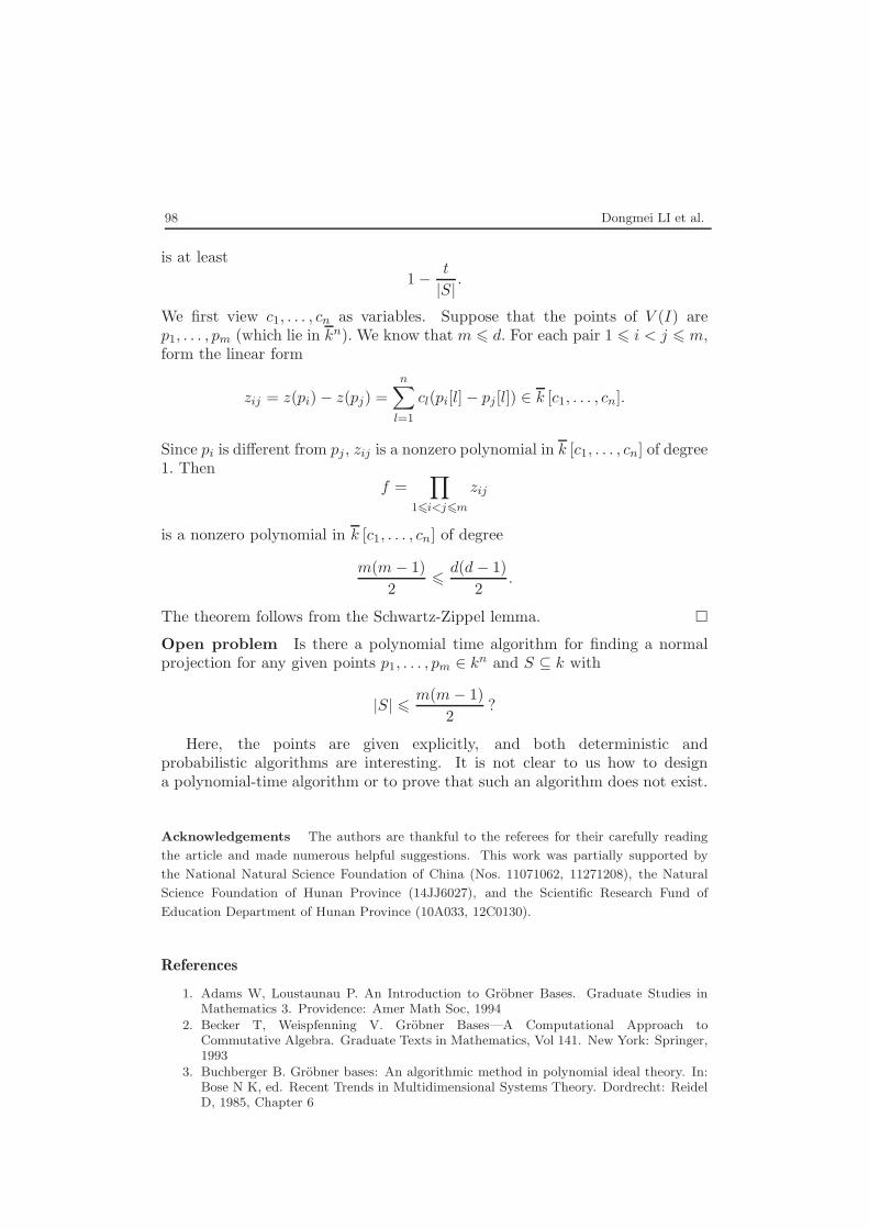
98 Dongmei LI et al.
is at least1 − t
|S| .
We first view c1, . . . , cn as variables. Suppose that the points of V (I) arep1, . . . , pm (which lie in kn). We know that m � d. For each pair 1 � i < j � m,form the linear form
zij = z(pi) − z(pj) =n∑
l=1
cl(pi[l] − pj[l]) ∈ k [c1, . . . , cn].
Since pi is different from pj, zij is a nonzero polynomial in k [c1, . . . , cn] of degree1. Then
f =∏
1�i<j�m
zij
is a nonzero polynomial in k [c1, . . . , cn] of degree
m(m − 1)2
� d(d − 1)2
.
The theorem follows from the Schwartz-Zippel lemma. �Open problem Is there a polynomial time algorithm for finding a normalprojection for any given points p1, . . . , pm ∈ kn and S ⊆ k with
|S| � m(m − 1)2
?
Here, the points are given explicitly, and both deterministic andprobabilistic algorithms are interesting. It is not clear to us how to designa polynomial-time algorithm or to prove that such an algorithm does not exist.
Acknowledgements The authors are thankful to the referees for their carefully reading
the article and made numerous helpful suggestions. This work was partially supported by
the National Natural Science Foundation of China (Nos. 11071062, 11271208), the Natural
Science Foundation of Hunan Province (14JJ6027), and the Scientific Research Fund of
Education Department of Hunan Province (10A033, 12C0130).
References
1. Adams W, Loustaunau P. An Introduction to Grobner Bases. Graduate Studies inMathematics 3. Providence: Amer Math Soc, 1994
2. Becker T, Weispfenning V. Grobner Bases—A Computational Approach toCommutative Algebra. Graduate Texts in Mathematics, Vol 141. New York: Springer,1993
3. Buchberger B. Grobner bases: An algorithmic method in polynomial ideal theory. In:Bose N K, ed. Recent Trends in Multidimensional Systems Theory. Dordrecht: ReidelD, 1985, Chapter 6
Normal projection: deterministic and probabilistic algorithms 99
4. Decker W, Greuel G -M, Pfister G. Primary decomposition: algorithms andcomparisons. In: Matzat B H, Greuel G -M, Hiss G, eds. Algorithmic Algebra andNumber Theory (Heidelberg, 1997). Berlin: Springer, 1999, 187–220
5. Gao S. Factoring multivariate polynomials via partial differential equations. MathComp, 2003, 72: 801–822
6. Gao S, Wan D, Wang M. Primary decomposition of zero-dimensional ideals over finitefields. Math of Comp, 2009, 78: 509–521
7. Garey M R, Johnson D S. Computers and Intractability: A Guide to the Theory ofNP-Completeness. Series of Books in the Mathematical Sciences. New York: W HFreeman, 1979
8. Grabe H -G. Minimal primary decomposition and factorized Grobner bases. ApplAlgebra Engrg Comm Comput, 1997, 8: 265–278
9. Greuel G -M, Pfister G. A Singular Introduction to Commutative Algebra. New York:Spinger-Verlag, 2002
10. Liu J, Li D. The λ-Grobner bases under polynomial composition. J Syst Sci Complex,2007, 20: 610–613
11. Liu J, Wang M. Homogeneous Grobner bases under composition. J Algebra, 2006, 303:668–676
12. Liu J, Wang M. Further results on homogeneous Grobner bases under composition.J Algebra, 2007, 315: 134–143
13. Monico C. Computing the primary decomposition of zero-dimensional ideals.J Symbolic Comput, 2002, 34: 451–459
14. Sausse A. A new approach to primary decomposition. J Symbolic Comput, 2001, 31:243–257
15. Schwartz J T. Fast probabilistic algorithms for verification of polynomial identities.J ACM, 1980, 27: 701–717
16. Steel A. Conquering inseparability:primary decomposition and multivariatefactorization over algebraic function fields of positive characteristic. J SymbolicComput, 2005, 40: 1053–1075
17. Takayama N. An approach to the zero recognition problem by Buchberger algorithm.J Symbolic Comput, 1992, 14: 265–282
18. Wang D. Decomposing algebraic varieties, Automated deduction in geometry (Beijing,1998). In: Lecture Notes Comput Sci, Vol 1669. Berlin: Springer, 1999, 180–206
19. Zippel R. Probabilistic algorithms for sparse polynomials. In: Proceedings of theInternational Symposium on Symbolic and Algebraic Computation. 1979, 216–226