Embed Size (px)
Citation preview

Normality, Modal Risk Level, and Exchange-Rate Jumps
By
Yoel Hecht* and Helena Pompushko**
2005.01 February 2005
2
Normality, Modal Risk Level, and Exchange-Rate Jumps
By
Yoel Hecht* and Helena Pompushko**
2005.01 February 2005
* Research Unit of the Banking Supervision Department, Bank of Israel, [email protected].
** Monetary Department, Bank of Israel, [email protected]
The views expressed in this article do not necessarily reflect those of the Bank of Israel.
© Bank of Israel
Those wishing to quote from this article may do so provided that the source is credited.
The Monetary Department, Bank of Israel, POB 780m 91007 Jerusalem
Catalogue no. 3111505001/0
http://www.bankisrael.gov.il

3
Normality, Modal Risk Level, and Exchange-Rate Jumps 1
Abstract
This article presents three indexes that may be used to examine the expected
exchange rate as reflected in trading in exchange-rate options. With these indexes one
may examine, on a daily basis, whether the expectations of exchange-rate change
were determined in a normal-distribution environment (hereinafter: the “N-Index”),
the modal risk level in the forex market (hereinafter: the “R-Index”), and the expected
direction and intensity of exchange-rate change in the event of an exchange-rate jump
(hereinafter: the “J-Index”).
We applied the indexes to daily trading in NIS/dollar exchange-rate options on
the Tel Aviv Stock Exchange. By analyzing the indexes for the October 2002–June
2004 period, we found that even though the NIS appreciated perceptibly against the
dollar (about 10 percent in the first half of 2003), the Israeli public continued to
associate the exchange-rate risk with depreciation: When the N-Index reflected an
abnormal market environment and the R-Index reflected a high modal risk level, the
J-Index reflected expectations of an exchange-rate jump only in the direction of
depreciation.
One of the possible reasons for the decrease in the forex sector’s contribution to
financing activity earnings in the Israeli banking system in 2003 (Supervisor of
Banks, 2004) may have been the rather severe misalignment between the expected
behavior of the exchange rate and its de facto behavior.
Key words: exchange rate, options, stochastic process, bi-lognormal distribution,
expectations, normality index, modal risk level index, exchange-rate jump index
1 We thank Akiva Offenbacher, Edi Azulai, Roy Stein and Asher Weingarten for their comments and
Menachem Brener for his contribution in calculating the VIX® index. We also thank the participants in
the Monetary Department and the Research Unit at the Banking Supervision Department for their
useful remarks and insights. Errors, if any, are the authors’ alone.
4
A. Introduction
The information implicit in the prices of sophisticated financial assets, especially
options, is of crucial interest to central banks as an input in the shaping of monetary
policy and to commercial banks in the management of foreign-exchange exposures.
This information reflects the market’s expectations about the future price of the
underlying asset upon the expiration of the options, since the income to be obtained
upon expiration depends on the price of the underlying asset at the time. Thus, option
prices depend on market expectations about the price of the underlying asset, the
standard deviation (Std) of it, the possibility of an abrupt change (“jump”) in the price
of the underlying asset, and additional parameters that are distribution indicative. For
example, options on the NIS/dollar exchange rate at various exercise prices may be
indicative not only of the average expected rate and its expected volatility but also of
the probabilities of various exchange-rate changes (Hecht and Stein, 2004).
The distribution, as observed by the markets, is clearly reflected in option prices
at various exercise prices. This is because option prices are highly sensitive to
expected developments in financial markets. The distribution of the future exchange
rate depends on the stochastic process that is typical of the exchange rate. Various
models that have attempted to monitor the stochastic process statistically have
undergone an evolutionary process, from the Random Walk to the mixed-diffusion-
jump process with conditional heteroscedasticity. Below we describe the models in
the order of their evolution.
1. Random Walk
The basic process used to describe exchange-rate behavior statistically is the Random
Walk, the continuous formulation of which is Brownian motion (Ross, 1996).
Krugman (1979) used this process to analyze an exchange-rate management regime
that relies partly on a target zone. Black and Scholes (1973) invoked it for the pricing
of options generally and Garman and Kohlhagen (1983) employed it for the pricing of
exchange-rate options specifically.
One of the premises of the basic process is that exchange-rate changes are
distributed normally. It was found, however, that this premise does not always obtain
and the distribution of changes in the prices of financial assets at large, and of those in
forex specifically, are better described by distribution with "fat tails" than by normal
5
distribution (Boothe and Glassman [1986]). Such findings led to studies that proposed
alternative exchange-rate distributions and more refined processes than the Random
Walk.
2. Mixed-Diffusion-Jump
The mixed-diffusion-jump, a combination of pure diffusion and discontinuous jumps,
is a more advanced development of Brownian motion. The process is defined by five
parameters: the expectation and variance of the diffusion process, the frequency of the
jumps, and the expectation and diffusion of the jumps (Booth and Akgiray [1988]).
Booth and Akgiray (1988) presented this process and showed that it is superior to
a mix of normal distributions in a model of exchange-rate changes in the pound
sterling, the Swiss franc, and the East German mark against the dollar is concerned.
Booth and Akgiray performed an empirical examination of exchange rates between
October 1976 and September 1985, when a “dirty” float regime was in effect. They
noted that monetary policy does have an effect on the formulation of exchange rates
but that exchange rates do not necessarily respond to this effect in the same way.
Their findings are consistent with the idea that the stochastic exchange-rate process
may change over time. In their estimation, markets respond to information in
consideration of policy targets such as money supply and interest rates, and that
structural changes may be related to inflation.
3. Autoregressive Conditional Heteroscedasticity
Autoregressive conditional heteroscedasticity is a process that describes the
development of exchange rate variance. Hecht (2000), basing himself on the Random
Walk model, compared several processes that describe the distribution of NIS/dollar
exchange-rate variance. The models examined were ARCH, GARCH, TARCH, and
EGARCH on daily exchange rates between December 1991 and June 1999. The
findings show that the model best suited to describing the development of NIS/dollar
exchange-rate variance is TARCH.
Johnston and Scott (2000) examined the extent to which the GARCH model
contributed to our understanding of the stochastic exchange-rate process and asked
whether more advanced GARCH processes were in fact promising. Their findings
show that the GARCH process is not promising and that there is a better formulation
that uses a standardization of the data by means of expectation and variance.
6
4. Mean Reversion, Conditional Heteroscedasticity, and Jump
Jiang (1998) presented an integration of the diffusion-jump process with
autoregressive conditional heteroscedasticity and added an element of mean
reversion. Arguing that there is some difficulty in estimating the model, he presented
an estimation of a parametric model formed from observed data by means of indirect
induction on the basis of simulations.
His results indicate that jumps are an important element in the exchange-rate
dynamic even when conditional heteroscedasticity (ARCH) and mean reversion are
taken into account. Models that take conditional heteroscedasticity into account,
however, tend to overestimate the frequency of the jumps and underestimate their
size.
The general parametric model estimated by Jiang follows:
(5) ( )( ) ( ) ( )( ) ( )λββσλµβα ttttttt dqYdWdtSdS 1/ 0 −++−=
where:
tS = asset price during period t.
tα = expected yield in the immediate term
2tσ = the immediate-term variance of the asset yield provided that a poissonian
jump does not take place
tW = the standard Gauss-Wiener process or the ordinary Brownian process
( )λtdq = an iid poissonian process
λ = the parameter of the poissonian process
( ) 1−βtY = random size of the jump when 0≥tY
0µ = expectations of jump size, i.e., [ ]1−tYE
( ) tt dWdq ,λ , statistically independent
( ) Θ∈= λµβθ ,, 0 = the parametric space that defines the function coefficients,
jump size, and the intensity of the poissonian process
Jiang phrased (5) in an alternative way:
( ) ( ) ( ) ( )λββσβµ tttttt dqYdWdtds ln++=
where:
tt Ss ln=
7
221
0 ttt σλµαµ −+=
The jump diffusion process described by Equation (6) is a Markov process with
one discontinuous parameter and one continuous one.
5. Summing Up the Processes
In sum, the evolution of the stochastic processes may be presented in the following
way:
(1) Black and Scholes Non-Jump Model (1973):
tt dWdtds σµ +=
(2) Merton's Jump Model (1976)
( ) ( )λσλµµ tttt dqYdWdtds ln0 ++−=
(3) Conditional Heteroscedasticity and Jump (in Jiang 1998)
( ) ( ) ( )λσσλµµ tttttt dqYdWsdtds ln0 +++−=
(4) Mean-Reversion, Conditional Heteroscedasticity, and Jump (in Jiang (1998))
( ) ( ) ( )λσσλµβµ ttttttt dqYdWsdtsds ln0 +++−−=
where,
),(ln 20 νµNiidYt ≈
For simplicity’s sake, this study assumes, in accordance with the model in
Merton (1976), that the changes in the underlying asset are continuous, random, and
accompanied by jumps, e.g., as in Ball and Torous (1983, 1985), Bates (1991) and
Beber and Brandt (2004) . Ball and Torous (1983) applied a model of jumps that
invokes this premise to forty-seven shares listed on the NYSE over 500 trading days
and found that 78 percent of the shares showed price jumps at a significance level of 1
percent.
Ball and Torous (1985) examined and compared two models for options pricing:
the Black and Scholes model—assuming that the changes in the underlying asset
develop in a continuous Random Walk pattern, meaning that the distribution function
is lognormal—and that of Merton (1976), which assumes that the underlying-asset
changes behave in a random-walk-jumps manner. Ball and Torous used the Bernoulli
version of the jump-diffusion model, in which jump size is not a stochastic variable.
In this case, the largest possible number of jumps during the life of the option is one.
Accordingly, one may describe the distribution function by mixing two lognormal
8
distributions. Ball and Torous found that the difference between the two models in the
shape of the distribution of changes in shares commonly traded on the NYSE is not
substantial. They noted, however, that the Merton model is more suitable for other
assets such as forex, in which price jumps are rare but large. Due to the paucity of the
daily data, our study presumes that the exchange rate jumps only once at the most.
Beber and Brandt (2004) examined the effect of regular and ordinary
macroeconomic announcements on the beliefs and preferences of players in the
American bond market by comparing short-term distributions before and after the
announcements. Using the standard diffusion-jump model, they found that the
announcements reduced the implicit uncertainty at the second moment of the
distribution irrespective of what the announcements had to say.
Distribution within a bi-lognormal framework is easy to estimate and elicits a
variety of parameters that provide information about the possible progression of the
underlying asset. Furthermore, as Aguilar and Hördahl (1991) note, this estimation
method is flexible: it may elicit a wide spectrum of types of distributions, including
the lognormal distribution as a private case. Within the framework of the bi-
lognormal distribution, four parameters (moments) that are typical of the expectations
may be calculated: expectation, standard deviation, kurtosis, and skewness.
Accordingly, the distribution that may be elicited within the bi-lognormal framework
is more realistic than a lognormal distribution.
This study is organized in the following way: Sections B and C describe the
methodology and the data. These sections, quoted from Hecht and Stein (2004), are
added because of their centrality in this article. Section D presents the index that we
use to examine normality of the foreign-exchange market. Section E presents an index
for modal risk level in the forex market. Section F presents an index of aberrant
exchange-rate change (jumps). Section G presents additional findings about the forex
market and compares the VIX® index with the implicit standard deviation as
calculated using the method in this study. Section H summarizes the study.
B. Methodology
1. General background
9
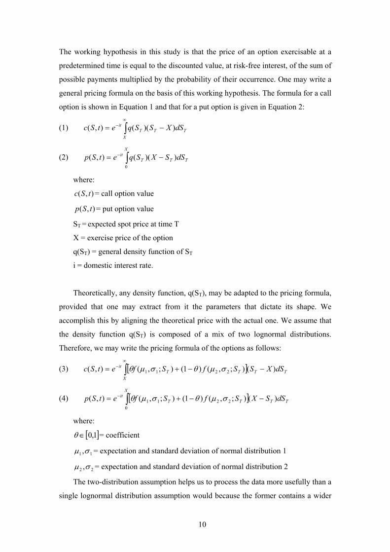
The working hypothesis in this study is that the price of an option exercisable at a
predetermined time is equal to the discounted value, at risk-free interest, of the sum of
possible payments multiplied by the probability of their occurrence. One may write a
general pricing formula on the basis of this working hypothesis. The formula for a call
option is shown in Equation 1 and that for a put option is given in Equation 2:
(1) ∫∞
− −=X
TTTit dSXSSqetSc ))((),(
(2) ∫ −= −X
TTTit dSSXSqetSp
0
))((),(
where:
),( tSc = call option value
),( tSp = put option value
ST = expected spot price at time T
X = exercise price of the option
q(ST) = general density function of ST
i = domestic interest rate.
Theoretically, any density function, q(ST), may be adapted to the pricing formula,
provided that one may extract from it the parameters that dictate its shape. We
accomplish this by aligning the theoretical price with the actual one. We assume that
the density function q(ST) is composed of a mix of two lognormal distributions.
Therefore, we may write the pricing formula of the options as follows:
(3) [ ]∫∞
− −−+=X
TTTTit dSXSSfSfetSc )();,()1();,(),( 2211 σµθσµθ
(4) [ ]∫ −−+= −X
TTTTit dSSXSfSfetSp
02211 )();,()1();,(),( σµθσµθ
where:
[ 1,0∈ ]θ = coefficient
11 ,σµ = expectation and standard deviation of normal distribution 1
22 ,σµ = expectation and standard deviation of normal distribution 2
The two-distribution assumption helps us to process the data more usefully than a
single lognormal distribution assumption would because the former contains a wider
10
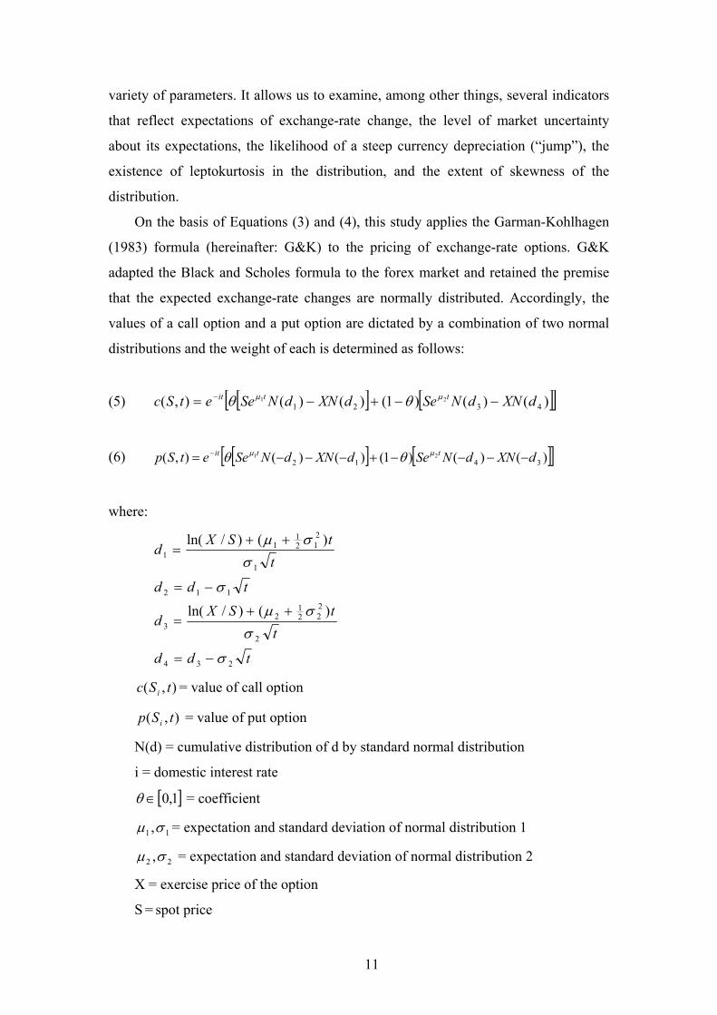
variety of parameters. It allows us to examine, among other things, several indicators
that reflect expectations of exchange-rate change, the level of market uncertainty
about its expectations, the likelihood of a steep currency depreciation (“jump”), the
existence of leptokurtosis in the distribution, and the extent of skewness of the
distribution.
On the basis of Equations (3) and (4), this study applies the Garman-Kohlhagen
(1983) formula (hereinafter: G&K) to the pricing of exchange-rate options. G&K
adapted the Black and Scholes formula to the forex market and retained the premise
that the expected exchange-rate changes are normally distributed. Accordingly, the
values of a call option and a put option are dictated by a combination of two normal
distributions and the weight of each is determined as follows:
(5) [ ] [ ][ ])()()1()()(),( 432121 dXNdNSedXNdNSeetSc ttit −−+−= − µµ θθ
(6) [ ] [ ][ ])()()1()()(),( 341221 dXNdNSedXNdNSeetSp ttit −−−−+−−−= − µµ θθ
where:
tdd
ttSX
d
tdd
ttSX
d
234
2
222
12
3
112
1
212
11
1
)()/ln(
)()/ln(
σ
σσµ
σ
σσµ
−=
++=
−=
++=
),( tSc i = value of call option
),( tSp i = value of put option
N(d) = cumulative distribution of d by standard normal distribution
i = domestic interest rate
[ 1,0∈ ]θ = coefficient
11 ,σµ = expectation and standard deviation of normal distribution 1
22 ,σµ = expectation and standard deviation of normal distribution 2
X = exercise price of the option
S = spot price
11
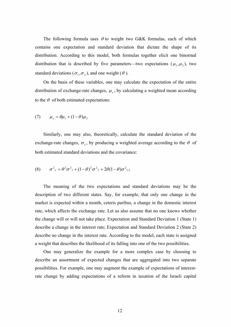
The following formula uses θ to weight two G&K formulas, each of which
contains one expectation and standard deviation that dictate the shape of its
distribution. According to this model, both formulas together elicit one binormal
distribution that is described by five parameters—two expectations ( 21 ,µµ ), two
standard deviations ( 21 ,σσ ), and one weight (θ ).
On the basis of these variables, one may calculate the expectation of the entire
distribution of exchange-rate changes, eµ , by calculating a weighted mean according
to the θ of both estimated expectations:
(7) 21 )1( µθθµµ −+=e
Similarly, one may also, theoretically, calculate the standard deviation of the
exchange-rate changes, eσ , by producing a weighted average according to the θ of
both estimated standard deviations and the covariance:
(8)
2,12
222
1222 )1(2)1( σθθσθσθσ −+−+=e
The meaning of the two expectations and standard deviations may be the
description of two different states. Say, for example, that only one change in the
market is expected within a month, ceteris paribus, a change in the domestic interest
rate, which affects the exchange rate. Let us also assume that no one knows whether
the change will or will not take place. Expectation and Standard Deviation 1 (State 1)
describe a change in the interest rate; Expectation and Standard Deviation 2 (State 2)
describe no change in the interest rate. According to the model, each state is assigned
a weight that describes the likelihood of its falling into one of the two possibilities.
One may generalize the example for a more complex case by choosing to
describe an assortment of expected changes that are aggregated into two separate
possibilities. For example, one may augment the example of expectations of interest-
rate change by adding expectations of a reform in taxation of the Israeli capital
12
market. This example, broader than the previous one, elicits four states.2 One may,
however, describe the four states by means of two groups that are differentiated by
their effect on exchange-rate development; each group has one expectation and one
standard deviation that are appropriate for all natural states in the group. Reality is
obviously more complex and the number of possible states is infinite. Therefore, the
meaning of the two expectations and standard deviations should be expanded to
represent two groups into which many states are aggregated.
The table below gives a condensed presentation of the variables in the model.
2 The states are: an interest rate increase with no change in taxation; an interest rate increase with a
change in taxation; an interest rate cut with no change in taxation; and an interest rate cut with a
change in taxation.
13
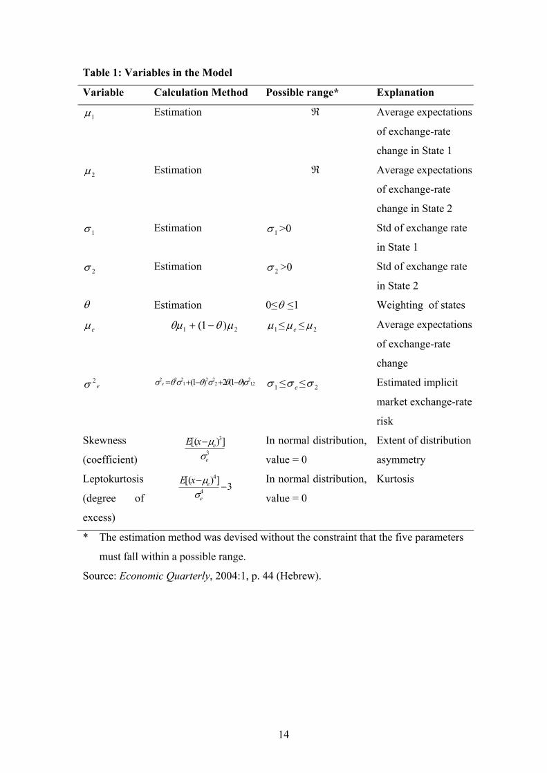
Table 1: Variables in the Model
Variable Calculation Method Possible range* Explanation
1µ Estimation ℜ Average expectations
of exchange-rate
change in State 1
2µ Estimation ℜ Average expectations
of exchange-rate
change in State 2
1σ Estimation 1σ >0 Std of exchange rate
in State 1
2σ Estimation 2σ >0 Std of exchange rate
in State 2
θ Estimation 0≤θ ≤1 Weighting of states
eµ 21 )1( µθθµ −+ 1µ ≤ eµ ≤ 2µ Average expectations
of exchange-rate
change
e2σ 2,1
22
221
222 )1(2)1( σθθσθσθσ −+−+=e 1σ ≤ eσ ≤ 2σ Estimated implicit
market exchange-rate
risk
Skewness
(coefficient) 3
3])[(
e
exEσµ− In normal distribution,
value = 0
Extent of distribution
asymmetry
Leptokurtosis
(degree of
excess)
3])[(4
4
−−
e
exEσµ In normal distribution,
value = 0
Kurtosis
* The estimation method was devised without the constraint that the five parameters
must fall within a possible range.
Source: Economic Quarterly, 2004:1, p. 44 (Hebrew).
14
2. Estimation
The method of estimating the double-log-normal distribution is based on the loss
function whose aim is to minimize the squared deviations between the prices of
options as assessed and priced by investors and the estimates obtained from the
pricing equation. The idea behind the method is to give a general description of the
options market by means of a limited number of variables (Hecht and Stein, 2004). In
practical terms, we are trying to find a set of variables which will minimize the
following objective function:
(9) { }∑ ⎥⎦
⎢⎣
+⎥⎦ p
Min=
⎤⎡ −⎤⎢⎣
⎡ −N
i i
ii
i
ii ppc
cc1
22
,,,,
ˆˆ2121 θσσµµ
Where:
ic – the price of a call option.
ip – the price of a put option.
ic - the price of a call option, estimated by equation 5.
ip - the price of a put option, estimated by equation 6.
The objective function is minimized by using the Gauss-Newton method, which is
based on changes in the gradient of the objective function. Use of this method
guarantees finding the global minimum by a complete search of the parameter space.
In the estimation there is no a priori constraint requiring the five parameters to be
within any possible range. Nevertheless, the values of the parameters obtained via this
estimation method are within reasonable bounds. Even so, the implied distribution on
the basis of a double log normal assumption sometimes has occasional spikes or a fat
tail, which seems to be a drawback in the estimation method. This happens when,
statistically, the estimated distribution is characterized as a one-log-normal
distribution and not as a double-log-normal distribution. Examining the significance
of the weight's parameter (θ) helps to overcome this drawback: If the weight's
parameter (θ) is significantly different from zero then the estimated distribution
should be based on only a one log-normal distribution.
15
C. Description of the Data
NIS/dollar options traded on the Tel Aviv Stock Exchange are typically series that are
differentiated by dates of maturity. In each series, both call and put options are traded
at several constant exercise prices. Since the exercise dates of the series are monthly,
at any point in time there are three series of options for the coming three months and
an additional series to the end of the next quarter. An additional series of options was
issued in 2002 and its expiration date was set at the end of the calendar year. The
determining exercise price of the options is the last price published by the Bank of
Israel before the exercise date, provided that the exercise date is a trading day on the
stock exchange. Options traded on the exchange are “shelf products” that have
homogeneous characteristics, unlike commercial bank options and Bank of Israel
options that are not typified by series. For the purposes of the model, which estimates
the prices of NIS/dollar options of identical maturities but at different exercise prices,
we used data pertaining to options traded on the Tel Aviv Stock Exchange.
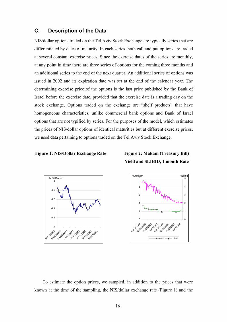
Figure 1: NIS/Dollar Exchange Rate
Figure 2: Makam (Treasury Bill)
Yield and $LIBID, 1 month Rate
0
2
4
6
8
10
01/10/2
002
01/01/2
003
01/04/2
003
01/07/2
003
01/10/2
003
01/01/2
004
01/04/2
004
01/07/2
004
0
1
2
3
4
5
makam libid
%libid%makam
4
4.2
4.4
4.6
4.8
5
01/10
/2002
01/01
/2003
01/04
/2003
01/07
/2003
01/10
/2003
01/01
/2004
01/04
/2004
01/07
/2004
NIS/Dollar
x xx
x
To estimate the option prices, we sampled, in addition to the prices that were
known at the time of the sampling, the NIS/dollar exchange rate (Figure 1) and the
16
NIS interest rate for the term of option life—the yield on Treasury bills redeemed at
approximately the time of option expiration (Figure 2). Notably, the dollar interest
rate (Figure 2) was not sampled here because it is endogenous in the model.
The option prices are sensitive to the price of the underlying asset (the NIS/dollar
exchange rate), market interest rates, and players’ expectations about the future
behavior of the underlying asset. Therefore, a change in one of these factors at any
time during the trading day is expected to affect the prices of the options, provided
that time for at least one transaction remains. Furthermore, when option prices are
sampled on the basis of transactions actually made, e.g., the closing price on the stock
exchange, it is not necessarily the case that transactions actually took place in all
options that were simultaneously listed at a given point in time. One option, or even
several options at different exercise prices, may have been traded earlier in the trading
day on the basis of information that had become irrelevant by closing time. An
alternative way to sample option prices solves the problem of temporal uniformity:
calculation of average bid and ask prices, as shown in the books of the stock exchange
at a predetermined point in time, and sampling of the dollar exchange rate and the
NIS interest rates at the same point in time.
In view of these characteristics of the data, we sampled, at a specific time in the
afternoon of each trading day, the best bid and ask prices for each option, as recorded
in the books of the stock exchange, along with the rest of the data—the known
NIS/dollar exchange rate and the Treasury bill yield at the time. The number of
options (put and call) at different exercise prices for which bids exist is not constant
throughout the trading day. On average, there are twenty options at different exercise
prices—all liquid options that exist in the market.
Most of the trading in options on the stock exchange is concentrated around
options whose exercise prices are close to the representative exchange rate and are of
short maturity. Therefore, one may obtain sufficiently extensive information by
sampling relatively short terms options — up to fifty days. At this maturity, the
trading volume is greater and spans a larger number of exercise prices; at the longest
maturities, in contrast, only three options at different exercise prices are traded and
such trading usually takes place around the representative NIS/dollar exchange rate.
17
These data gave us a basis for estimating the expected distribution of the
NIS/dollar exchange rate, on each trading day, with the help of the bi-lognormal
distribution function.
The data included trading days between October 2002 and May 2004—410 days
in all—and 9,818 series of options (see Appendix A).
To perform the estimation, we used only observations for which the implicit
standard deviation ranged from 2 percent to 20 percent. We treated other observations
as aberrant and deleted them. Notably, the deletion hardly affected the nature of the
estimated distribution (lognormal or bi-lognormal) but did affect the estimates of the
parameters.
There are four interrelated approaches to the distribution of the future exchange
rate (Hecht and Stein, 2004):
(1) The actual distribution of the future exchange rate is the only distribution
that describes the behavior of the future exchange rate. This distribution cannot be
identified.
(2) The subjective distribution of each player in the market is the distribution
by which the players price transactions in derivatives. This distribution does not
necessarily correspond to that of the actual future exchange rate; it may include
subjective elements related to decision-making under risk conditions, as Kahneman
and Tversky’s Prospect Theory (1979) and Levy and Levy (2002) notes. Furthermore,
since various market players observe different “actual” distributions, the distribution
observed by the various players is a weighting of these distributions. Because players
are strongly influenced by the distributions that they observe, however, these
distributions may be of greater interest than the actual distribution.
(3) A distribution based on a theoretical assumption about exchange-rate
behavior is a function (or a set of functions) that describes the exchange-rate
distribution. The distribution may be derived from a stochastic theoretical process
and/or from a theoretical process of market equilibration. This distribution may not
describe reality with exactitude but is usually more convenient to use in analyzing the
behavior of the exchange rate. Thus, for example, Krugman (1979) assumes a
theoretical exchange-rate process and, on this basis, presents a regime of exchange-
rate flexibility within a range.
18
(4) Estimated exchange-rate distribution—average of subjective
distributions is the result of empirical examination of the market data by means of
various techniques. The result pertains to a specific period in time, a predetermined
frequency, specific currencies, etc.
The various approaches are interrelated. The actual distribution of the exchange
rate (1) affects the distribution observed by the players (2). However, changes in
players’ expectations may affect the actual distribution (1). The methods that players
use to shape the distributions that they observe (2) are usually an estimated
distribution of the exchange rate (4) and a distribution based on a theoretical premise
(3).
We may improve the estimated distribution by examining these interrelations.
One well-known phenomenon is the “volatility smile”: the estimated distribution
indicates that the farther the exercise price is from the money, the larger the implicit
standard deviation of the options is. The “smile” phenomenon is elicited by using the
Black and Scholes formula, which bases the exchange-rate distribution on the
theoretical assumption (3) of a lognormal distribution. The “smile” effect clashes with
the theoretical premise of our model. By implication, the exchange-rate distribution
that the players observe (2) is not lognormal. Consequently, various ways of
improving the theoretical distribution have been proposed.
A regime of exchange-rate flexibility within a trading band, such as Israel’s, is
expected to affect the exchange-rate distribution as observed by the market players.
The closer the exchange rate is to the boundaries of the range, the stronger the effect
on the distribution is expected to be. Campa, Chang, and Refalo (1998) examined the
credibility of Brazil’s exchange-rate trading band during 1994–1997 on the basis of
options and found that credibility increased after 1996. Our study did not examine the
effect of the band on exchange-rate distribution. Israel’s trading band evidently had
little effect on the distribution as long as the NIS/currency-basket exchange rate was
relatively far from the bounds of the band. In late 1996, during the first half of 1997,
and in the first half of 1998, however, the rate verged on the lower bound. Although
the market data during the sampling period of this study showed a negligible
likelihood of returning to the vicinity of the lower bound, this may change in the
future. In such a state, the bi-lognormal distribution will reflect the distribution of the
exchange rate more credibly and the exchange rate will be more indicative of the
19
credibility of Israeli’s exchange-rate regime in investors’ eyes. When the exchange
rate stays within the band but approaches one of its bounds, the bi-lognormal
distribution will be indicative both of the probability of breaching the bound in an
exchange rate “jump” and the size of the jump as an indication that the exchange-rate
policy lacks credibility.
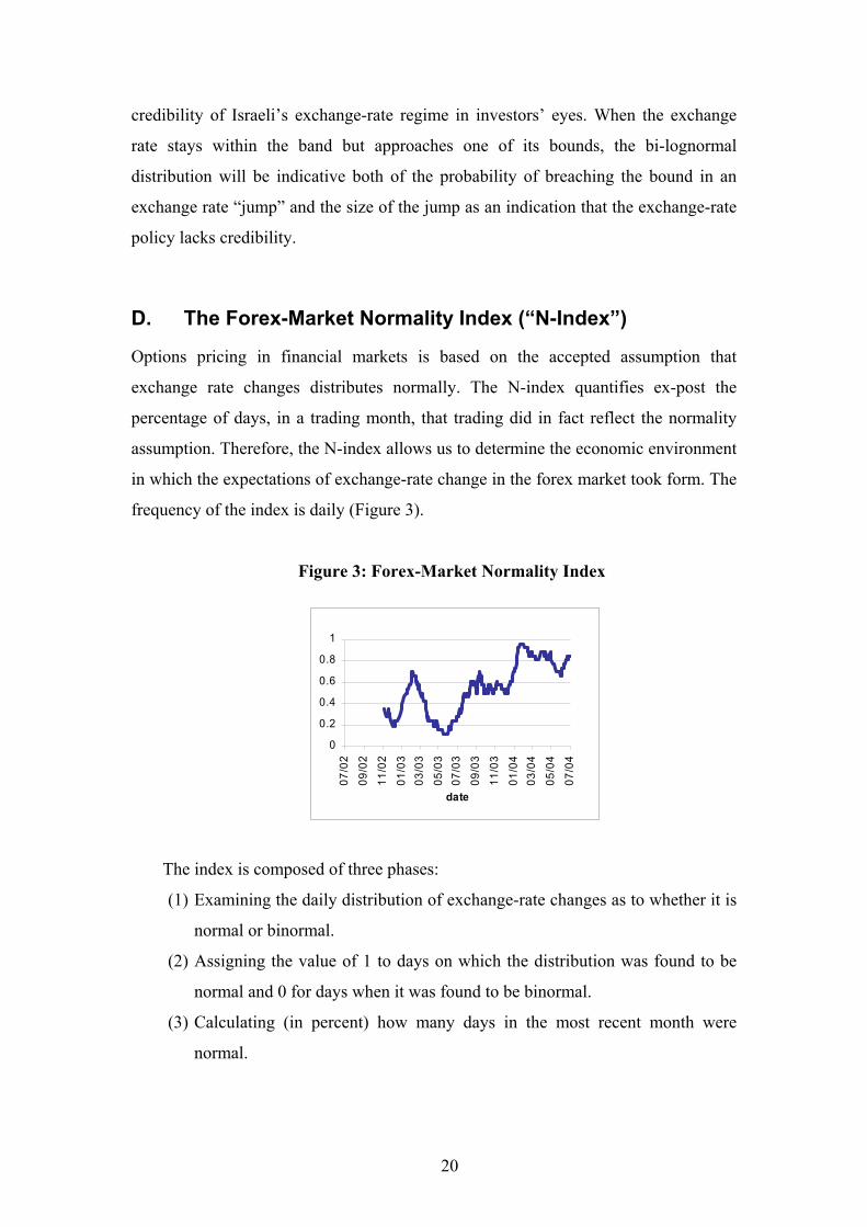
D. The Forex-Market Normality Index (“N-Index”)
Options pricing in financial markets is based on the accepted assumption that
exchange rate changes distributes normally. The N-index quantifies ex-post the
percentage of days, in a trading month, that trading did in fact reflect the normality
assumption. Therefore, the N-index allows us to determine the economic environment
in which the expectations of exchange-rate change in the forex market took form. The
frequency of the index is daily (Figure 3).
Figure 3: Forex-Market Normality Index
0
0.2
0.4
0.6
0.8
1
07/0
2
09/0
2
11/0
2
01/0
303
/03
05/0
307
/03
09/0
3
11/0
3
01/0
403
/04
05/0
4
07/0
4
date
The index is composed of three phases:
(1) Examining the daily distribution of exchange-rate changes as to whether it is
normal or binormal.
(2) Assigning the value of 1 to days on which the distribution was found to be
normal and 0 for days when it was found to be binormal.
(3) Calculating (in percent) how many days in the most recent month were
normal.
20

Phase 1 is performed by means of four tests that allow us to determine whether,
at 10 percent statistical significance, θ , 1-θ , Std1, and Std2 are other than zero (see
Appendix B). If one of these is not significantly different from 0, the exchange-rate
change is normal. If all are different from 0, the distribution of the exchange-rate
change is composed of two normal distributions and that of the exchange rate itself is
bi-lognormal. Notably, the statistical test is incomplete because it allows only two
possibilities of exchange-rate distribution even though additional possibilities may
exist in other time ranges. This is why we call our test of normality an “index” and
not a “test.” The values that this index may receive range from 0 percent to 100
percent.
Analysis of the index during the recent period shows that it changed perceptibly,
climbing from 10 percent normal distribution days in the middle of 2003 to almost
100 percent in early 2004. These changes are consistent with stylized facts that are
familiar from forex-market and Nis/dollar exchange-rate developments during that
time: an increase in nonresident capital inflows in the first half of 2003 and a halt to
the inflow and reversal of the exchange-rate trend in late June (Supervisor of Banks,
2004).
Figure 4: Implicit Std of Call Options less Put Options Versus the N-Index
-0.01
-0.005
0
0.005
0.01
0.015
0.02
0 0.2 0.4 0.6 0.8 1
N מדד
ה ומגל הקןהת
טיי
סבין
ת ביש פרה
ת מולוהג
לו אן
לca
ll ותציופבא
put ת
ציוופבא
Impl
icit
Std
of C
all O
ptio
ns
less
Put
Opt
ions
N index
21
We examined the N-Index in an additional direction by calculating the implicit
standard deviation in call options and put options separately. At times of normal
exchange-rate distribution, we expected the separately calculated standard deviations
to be equal and, therefore, expected the difference between the calculations to be
closer to 0. We posited the difference against the N-Index (Figure 4) and found, as
expected, a negative correspondence between the two series. That is, when the
distribution was normal—when the N-Index was high—the implicit standard
deviations of call options and put options were similar and, therefore, the difference
between them was small, and vice versa.
Notably, we did not expect to find, in “abnormal” times, that the difference
between the implicit standard deviations of call options and put options would go in
one direction most of the time. The direction obtained during “abnormal” times was
positive. The explanation lies in a phenomenon typical of the Israeli economy: the
public associates exchange-rate risk with depreciation (Hecht, 2000). Therefore, when
risk increases, the market assigns in the right tail of the distribution a higher price to
call options than to put options in the same distance in the left tail, as reflected in a
higher implicit standard deviation. This correspondence was expressed in the intensity
of the pro-depreciation skew of the distribution during most of the sample period.
The depreciation expectations calculated by the method used in this study
correspond to the financial behavior of Israel’s private sector. In the first half of 2000,
the business sector had a net asset surplus in forex. In the event of currency
appreciation, however, this sector is liable to sustain a considerable loss.
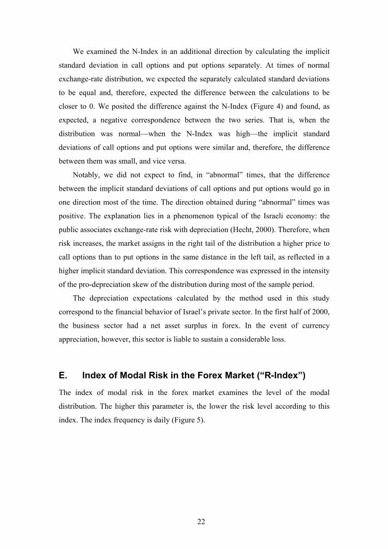
E. Index of Modal Risk in the Forex Market (“R-Index”)
The index of modal risk in the forex market examines the level of the modal
distribution. The higher this parameter is, the lower the risk level according to this
index. The index frequency is daily (Figure 5).
22
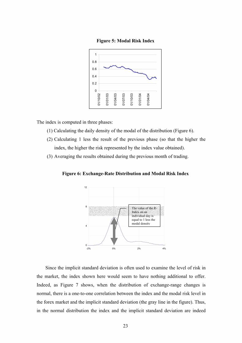
Figure 5: Modal Risk Index
0
0.2
0.4
0.6
0.8
1
01/1
0/02
01/0
1/03
01/0
4/03
01/0
7/03
01/1
0/03
01/0
1/04
01/0
4/04
The index is computed in three phases:
(1) Calculating the daily density of the modal of the distribution (Figure 6).
(2) Calculating 1 less the result of the previous phase (so that the higher the
index, the higher the risk represented by the index value obtained).
(3) Averaging the results obtained during the previous month of trading.
Figure 6: Exchange-Rate Distribution and Modal Risk Index
0
4
8
12
-2% 0% 2% 4%
צפיפות
The value of the R-Index on an individual day is equal to 1 less the modal density
Since the implicit standard deviation is often used to examine the level of risk in
the market, the index shown here would seem to have nothing additional to offer.
Indeed, as Figure 7 shows, when the distribution of exchange-range changes is
normal, there is a one-to-one correlation between the index and the modal risk level in
the forex market and the implicit standard deviation (the gray line in the figure). Thus,
in the normal distribution the index and the implicit standard deviation are indeed
23
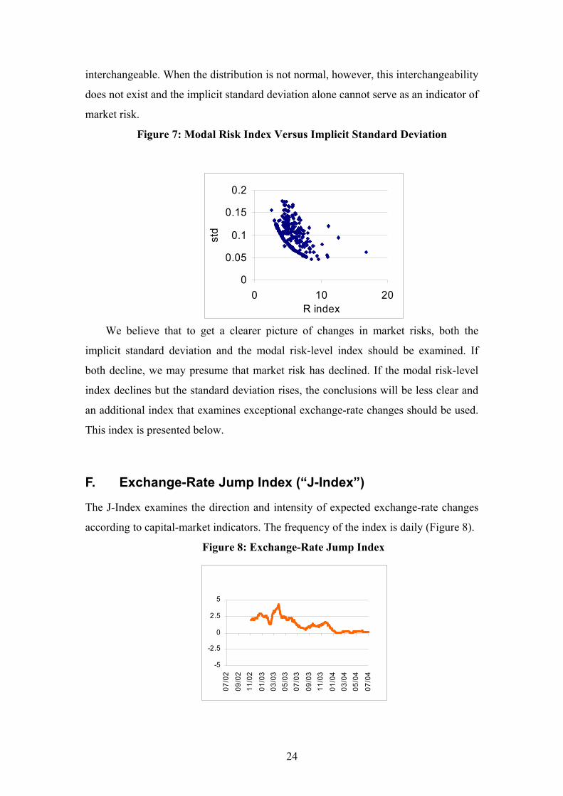
interchangeable. When the distribution is not normal, however, this interchangeability
does not exist and the implicit standard deviation alone cannot serve as an indicator of
market risk.
Figure 7: Modal Risk Index Versus Implicit Standard Deviation
0
0.05
0.1
0.15
0.2
0 10R index
std
20
We believe that to get a clearer picture of changes in market risks, both the
implicit standard deviation and the modal risk-level index should be examined. If
both decline, we may presume that market risk has declined. If the modal risk-level
index declines but the standard deviation rises, the conclusions will be less clear and
an additional index that examines exceptional exchange-rate changes should be used.
This index is presented below.
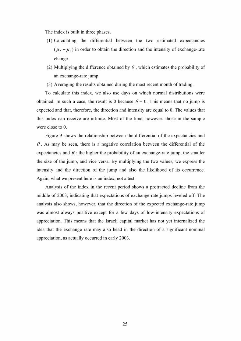
F. Exchange-Rate Jump Index (“J-Index”)
The J-Index examines the direction and intensity of expected exchange-rate changes
according to capital-market indicators. The frequency of the index is daily (Figure 8).
Figure 8: Exchange-Rate Jump Index
-5
-2.5
0
2.5
5
07/0
2
09/0
211
/02
01/0
303
/03
05/0
307
/03
09/0
311
/03
01/0
403
/04
05/0
4
07/0
4
24
The index is built in three phases.
(1) Calculating the differential between the two estimated expectancies
( 12 µµ − ) in order to obtain the direction and the intensity of exchange-rate
change.
(2) Multiplying the difference obtained by θ , which estimates the probability of
an exchange-rate jump.
(3) Averaging the results obtained during the most recent month of trading.
To calculate this index, we also use days on which normal distributions were
obtained. In such a case, the result is 0 because θ = 0. This means that no jump is
expected and that, therefore, the direction and intensity are equal to 0. The values that
this index can receive are infinite. Most of the time, however, those in the sample
were close to 0.
Figure 9 shows the relationship between the differential of the expectancies and
θ . As may be seen, there is a negative correlation between the differential of the
expectancies and θ : the higher the probability of an exchange-rate jump, the smaller
the size of the jump, and vice versa. By multiplying the two values, we express the
intensity and the direction of the jump and also the likelihood of its occurrence.
Again, what we present here is an index, not a test.
Analysis of the index in the recent period shows a protracted decline from the
middle of 2003, indicating that expectations of exchange-rate jumps leveled off. The
analysis also shows, however, that the direction of the expected exchange-rate jump
was almost always positive except for a few days of low-intensity expectations of
appreciation. This means that the Israeli capital market has not yet internalized the
idea that the exchange rate may also head in the direction of a significant nominal
appreciation, as actually occurred in early 2003.
25
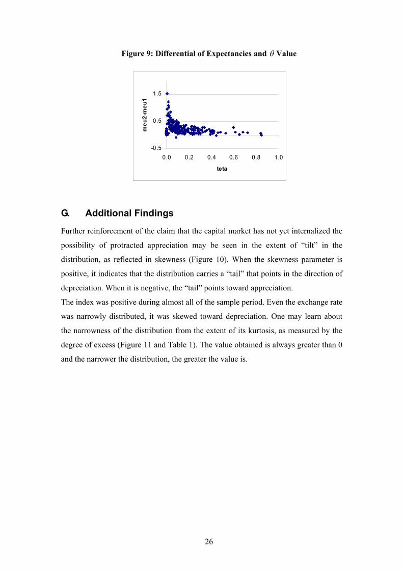
Figure 9: Differential of Expectancies and θ Value
-0.5
0.5
1.5
0.0 0.2 0.4 0.6 0.8 1.0
teta
meu
2-m
eu1
G. Additional Findings
Further reinforcement of the claim that the capital market has not yet internalized the
possibility of protracted appreciation may be seen in the extent of “tilt” in the
distribution, as reflected in skewness (Figure 10). When the skewness parameter is
positive, it indicates that the distribution carries a “tail” that points in the direction of
depreciation. When it is negative, the “tail” points toward appreciation.
The index was positive during almost all of the sample period. Even the exchange rate
was narrowly distributed, it was skewed toward depreciation. One may learn about
the narrowness of the distribution from the extent of its kurtosis, as measured by the
degree of excess (Figure 11 and Table 1). The value obtained is always greater than 0
and the narrower the distribution, the greater the value is.
26
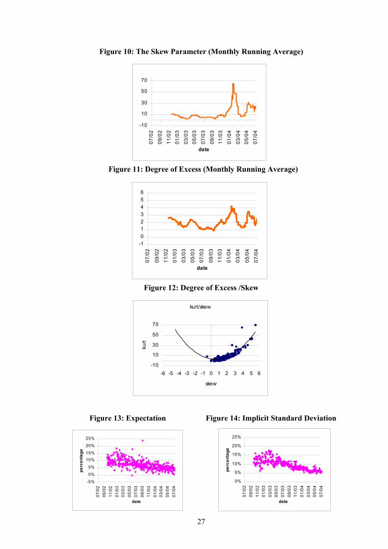
Figure 10: The Skew Parameter (Monthly Running Average)
-10
10
30
50
70
07/0
2
09/0
2
11/0
201
/03
03/0
305
/03
07/0
3
09/0
311
/03
01/0
4
03/0
405
/04
07/0
4
date
Figure 11: Degree of Excess (Monthly Running Average)
-10123456
07/0
2
09/0
2
11/0
2
01/0
3
03/0
3
05/0
3
07/0
3
09/0
3
11/0
3
01/0
4
03/0
4
05/0
4
07/0
4
date
Figure 12: Degree of Excess /Skew
kurt/skew
-10
10
30
50
70
-6 -5 -4 -3 -2 -1 0 1 2 3 4 5 6
skew
kurt
Figure 13: Expectation Figure 14: Implicit Standard Deviation
0%
5%
10%
15%
20%
25%
07/0
209
/02
11/0
201
/03
03/0
305
/03
07/0
309
/03
11/0
301
/04
03/0
405
/04
07/0
4
date
perc
enta
ge
-5%
0%
5%
10%15%
20%
25%
07/0
209
/02
11/0
201
/03
03/0
305
/03
07/0
309
/03
11/0
301
/04
03/0
405
/04
07/0
4
date
perc
enta
ge
27

In principle, no correlation is expected between skewness and kurtosis; it may be
negative or positive (the black theoretical line in Figure 12). Figure 12 shows,
however, that the capital market did elicit a significant correlation: the narrower the
distribution (the less the kurtosis), the more skewed it was. This indicates that the
capital market has not yet internalized the fact that the exchange rate can also move
toward a significant nominal appreciation, such as the one that occurred in early 2003.
The direction of the expected exchange-rate jump was almost always positive—
except for a few days when it did turn toward appreciation but at low intensity.
Figures 13 and 14 show the expectation and standard deviation of the expected
exchange rate. Both parameters declined during the period reviewed.
During 1993, the Chicago Board Option Exchange (CBOE®) introduced the
VIX® index, a nonparametric method to calculate the implicit standard deviation of
options. The index became a yardstick for the volatility of the American stock market
(CBOE [2003]). Since volatility sometimes reflects exceptional financial changes, the
VIX® index has evolved into an “investor-fear index” as well. With this in mind, we
applied the VIX® index to the forex options data. Afterwards we compared the VIX®
index results with the implicit standard deviation of options as calculated on the basis
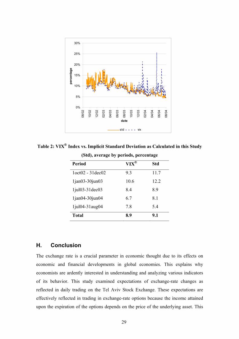
of the methods shown in this study (Figure 15). As Figure 15 and Table 2 show, the
behavior of the VIX® index is perceptibly different from the implicit standard
deviation as calculated in this study. We believe that our method is preferable to the
VIX® index as an "investor fear index" for the Israeli forex market from two
standpoints. Firstly, from an economic standpoint, the index in this study provides a
better reflection of periods of calm and turmoil in the Israeli forex market. Secondly,
form a statistical standpoint, the loss function of the estimation elicited a lower value
for the standard deviation in this study (3.7) than for the VIX® index (63.3).
Figure 15: VIX® Index Versus Implicit Standard Deviation (Std) as
Calculated in this paper
28
0%
5%
10%
15%
20%
25%
30%
08/0
2
10/0
2
12/0
2
02/0
3
04/0
3
06/0
3
08/0
3
10/0
3
12/0
3
02/0
4
04/0
4
06/0
4
08/0
4
date
perc
enta
ge
std vix
Table 2: VIX® Index vs. Implicit Standard Deviation as Calculated in this Study
(Std), average by periods, percentage
Period VIX® Std
1oct02 - 31dec02 9.3 11.7
1jan03-30jun03 10.6 12.2
1jul03-31dec03 8.4 8.9
1jan04-30jun04 6.7 8.1
1jul04-31aug04 7.8 5.4
Total 8.9 9.1
H. Conclusion
The exchange rate is a crucial parameter in economic thought due to its effects on
economic and financial developments in global economies. This explains why
economists are ardently interested in understanding and analyzing various indicators
of its behavior. This study examined expectations of exchange-rate changes as
reflected in daily trading on the Tel Aviv Stock Exchange. These expectations are
effectively reflected in trading in exchange-rate options because the income attained
upon the expiration of the options depends on the price of the underlying asset. This
29
study describes these expectations as the estimated distribution of the exchange rate.
The distribution estimated in this study is of exchange-rate changes on the assumption
of bi-lognormal distribution of the rate itself. This premise is consistent with the
stochastic process proposed by Merton (1976), according to which changes in the
underlying asset are continuous, random, and accompanied by jumps. Due to the
small number of observations per day, we assumed in this study that the exchange rate
is expected to undergo no more than one jump during the process.
Using data on options trading on the Tel Aviv Stock Exchange, we estimated 410
daily distributions between October 2002 and June 2004 and found that the direction
of the expected jump in the NIS/dollar exchange rate was almost always positive—
except for a few days when it pointed toward appreciation but at a low intensity. We
adduced from this that the Israeli capital market has still not internalized the
awareness that the exchange rate can also move in the direction of significant nominal
appreciation, as indeed happened in early 2003.
One of the factors behind the decline in the contribution of the forex sector to
Israeli banks’ financing activity earnings in 2003 (Supervisor of Banks [2004]) may
have been the rather severe misalignment between the expectations of a currency
depreciation and the appreciation that actually occurred.
30
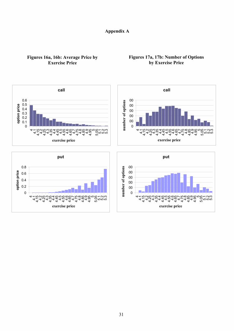
Appendix A
Figures 16a, 16b: Average Price by
Exercise Price Figures 17a, 17b: Number of Options
by Exercise Price
call
0100200300400500
44.
14.
15 4.2
4.25 4.3
4.35 4.4
4.45 4.5
4.55 4.6
4.65 4.7
4.75 4.8
4.85 4.9
4.95 5
5.05 5.1
5.2
5.3
Exercise Price
Num
ber o
f Opt
ions
put
0100200300400500
44.
14.
15 4.2
4.25 4.3
4.35 4.4
4.45 4.5
4.55 4.6
4.65 4.7
4.75 4.8
4.85 4.9
4.95 5
5.05 5.1
5.2
5.3
eExercise Pric
Num
ber o
f Opt
ions
num
ber
of o
ptio
ns
num
ber
of o
ptio
ns
exercise price
exercise price
call
00.10.20.30.40.50.6
44.
14.
15 4.2
4.25 4.3
4.35 4.4
4.45 4.5
4.55 4.6
4.65 4.7
4.75 4.8
4.85 4.9
4.95 5
5.05 5.1
5.2
5.3
Exercise Price
optio
n pr
ice
put
0
0.2
0.4
0.6
0.8
44.
14.
15 4.2
4.25 4.3
4.35 4.4
4.45 4.5
4.55 4.6
4.65 4.7
4.75 4.8
4.85 4.9
4.95 5
5.05 5.1
5.2
5.3
e
optio
n pr
ice
Exercise Pricexercise price
exercise price
31
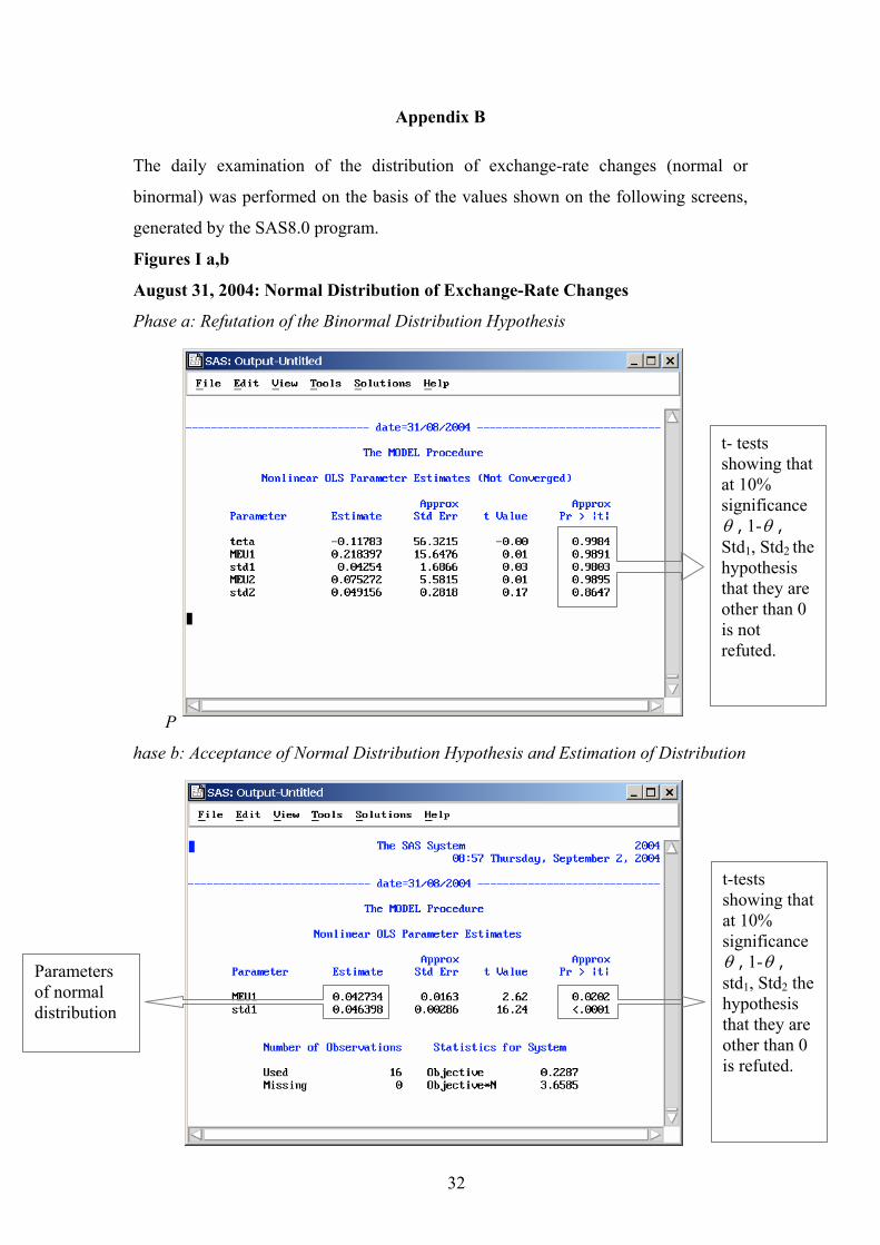
Appendix B
The daily examination of the distribution of exchange-rate changes (normal or
binormal) was performed on the basis of the values shown on the following screens,
generated by the SAS8.0 program.
Figures I a,b
August 31, 2004: Normal Distribution of Exchange-Rate Changes
Phase a: Refutation of the Binormal Distribution Hypothesis
P
hase b: Acceptance of Normal Distribution Hypothesis and Estimation of Distribution
t- tests showing that at 10% significance θ , 1-θ , Std1, Std2 the hypothesis that they are other than 0 is not refuted.
Parameters of normal distribution
t-tests showing that at 10% significance θ , 1-θ , std1, Std2 the hypothesis that they are other than 0 is refuted.
32
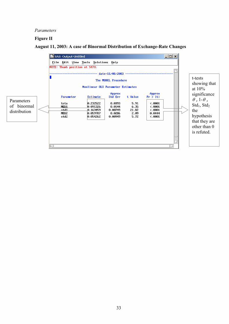
Parameters
Figure II
August 11, 2003: A case of Binormal Distribution of Exchange-Rate Changes
Parameters of binormal distribution
t-tests showing that at 10% significance θ , 1-θ , Std1, Std2 the hypothesis that they are other than 0 is refuted.
33

Bibliography
Hebrew Sources
Hecht, Y. (2000), “Estimating the Standard Deviation of Daily Changes in the
NIS/Dollar Exchange Rate by Means of the GARCH Model,” Bank of Israel,
internal paper.
Hecht, Y., and R. Stein (2004), “Estimating the Implicit Expected Distribution of the
NIS/Dollar Exchange Rate in Option Prices,” Economic Quarterly 2004 (1) 36–
60.
Supervisor of Banks (2004), 2003 Annual Survey, 147-148.
Ruthenberg, D. (2002), Banking Management in Israel, Keter, Jerusalem, 274–283.
English Sources
Aguilar, J., and P. Hördahl (1991), “Option Prices and Market Expectations,”
Monetary and Exchange Rate Policy Department Quarterly Review, 1, 43–70.
Ball, C. A., and W. N. Torous (1983), “A Simplified Jump Process for Common
Stock Returns,” Journal of Financial and Quantitative Analysis, 18, No. 1, 53–65.
Ball, C. A., and W. N. Torous (1985), “On Jumps in common Stock Prices and Their
Impact on Call Option Pricing,” The Journal of Finance, XL No. 1, 155–173.
Bates, D. S. (1991), “The Crash of ‘87: Was It Expected? The Evidence from Option
Markets,” The Journal of Finance, 46, 1009-1044.
Beber, A., and M. Brandt (2003), “The Effect of Macroeconomic News on Beliefs
and Preferences: Evidence from the Options Market,” NBER Working Paper No.
9914.
Black, F., and M. Scholes (1973), “The Pricing of Options and Corporate Liabilities,”
Journal of Political Economy 81 (May-June), pp. 637-654.
Booth, G., and V. Akgiray (1988), “Mixed Diffusion-Jump Process Modeling of
Exchange Rate Movements,” The Review of Economics and Statistics, Vol. 70,
631–637.
Boothe, P., and D. Glassman (1986), “The Statistical Distribution of Exchange Rates:
Empirical Evidence and Economic Implications,” Journal of International
Economics 22, 297–319.
34
Campa, J. M., K. P. H. Chang, and J. F. Refalo (1998), “An Options-Based Analysis
of Emerging Market Exchange Rate Expectations: Brazil’s Real Plan, 1994–
1997,” Estimating and Interpreting Probability Density Functions, proceedings of
workshop held at BIS on June 14, 1999, 211–234.
Chicago Board Options Exchange (CBOE) (2003), “The New CBOE Volatility
Index—VIX,” available at www.cboe.com/micro/vix/vixwhite.pdf.
Garman, M. B., and S. W. Kohlhagen (1983), “Foreign Currency Option Values,”
Journal of International Money and Finance, 2, 231–237.
Jiang, G. J. (1998), “Jump-Diffusion Model of Exchange Rate Dynamics—Estimation
via Indirect Inference,” available at www.ub.rug.nl/eldoc/som/a/98A40/98a40.pdf
Johnston, K., and E. Scott (2000), “GARCH Model and the Stochastic Process
underlying Exchange Rate Price Changes,” Journal of Financial and Strategic
Decisions, Vol. 13.
Krugman, P. (1979), “Target Zones and Exchange Rate Dynamics,” NBER Working
Paper No. 2481, January.
Kahneman, D., and A. Tversky (1979), “Prospect Theory: An Analysis of Decision
Under Risk,” Econometrica, 47, 263–291.
Levi, M., and H. Levi (2002), “Prospect Theory: Much Ado about Nothing?”
Management Science, 48, 870–873.
Merton, R. (1976), “Option Pricing When Underlying Stock Returns are
Discontinuous,” Journal of Financial Economics 3, 125–144.
Ross S. M. (1996), Stochastic Process, John Wiley & Sons, second edition.
35
Monetary Studies עיונים מוניטריים מודל לבחינת ההשפעה של המדיניות המוניטרית –אלקיים ' ד, אזולאי' א1999.01
על 1996 עד 1988, האינפלציה בישראל
השערת הניטרליות של שיעור האבטלה ביחס –סוקולר ' מ, אלקיים' ד1999.021998 עד 1990, בחינה אמפירית–לאינפלציה בישראל
2000.01M. Beenstock, O. Sulla – The Shekel’s Fundamental Real Value
2000.02O. Sulla, M. Ben-Horin –Analysis of Casual Relations and Long and Short-term Correspondence between Share Indices in Israel and the United States
2000.03Y. Elashvili, M. Sokoler, Z. Wiener, D. Yariv – A Guaranteed-return Contract for Pension Funds’ Investments in the Capital Market
חוזה להבטחת תשואת רצפה –סוקולר ' מ, יריב' ד, וינר' צ, אלאשווילי' י2000.04 לקופות פנסיה תוך כדי הפנייתן להשקעות בשוק ההון
מודל לניתוח ולחיזוי– יעד האינפלציה והמדיניות המוניטרית –אלקיים ' ד2001.01
תחות מול מדינות מפו: דיסאינפלציה ויחס ההקרבה–ברק ' ס, אופנבכר' ע2001.02 מדינות מתעוררות
2001.03D. Elkayam – A Model for Monetary Policy Under Inflation Targeting: The Case of Israel
אמידת פער התוצר ובחינת השפעתו על –אלאשווילי ' י, רגב' מ, אלקיים' ד2002.01 האינפלציה בישראל בשנים האחרונות
ער החליפין הצפוי באמצעות אופציות אמידת ש–שטיין ' ר2002.02 Call - על שער ה Forward
2003.01
הסחירות של חוזים עתידיים - מחיר אי–קמרה ' א, קהן' מ, האוזר' ש, אלדור' ר )בשיתוף הרשות לניירות ערך(
2003.02 R. Stein - Estimation of Expected Exchange-Rate Change Using Forward Call Options
דולר - אמידת ההתפלגות הצפויה של שער החליפין שקל–הכט ' י, שטיין' ר 2003.03 הגלומה במחירי האופציות
2003.04 D. Elkayam – The Long Road from Adjustable Peg to Flexible Exchange Rate Regimes: The Case of Israel
2003.05 R. Stein, Y. Hecht – Distribution of the Exchange Rate Implicit in Option Prices: Application to TASE
מודל לחיזוי הגירעון המקומי של הממשלה–ארגוב ' א 2004.01
רמת סיכון שכיחה ושינוי חריג בשער החליפין, נורמליות–פומפושקו ' וה, הכט' י 2004.02
2004.03 D.Elkayam ,A.Ilek – The Information Content of Inflationary Expectations Derived from Bond Prices in Israel
36
התפלגות , דולר- ההתפלגות הצפויה של שער החליפין שקל–שטיין . ר 2004.04 פרמטרית הגלומה באופציות מטבע חוץ -א
2005.01 Y. Hecht, H. Pompushko – Normality, Modal Risk Level, and Exchange-Rate Jumps
המחלקה המוניטרית–בנק ישראל
91007 ירושלים 780ד "ת
Bank of Israel – Monetary DepartmentPOB 780 91007 Jerusalem, Israel
37