Embed Size (px)
Citation preview
Notas de Aula (Gibbons, 1992) - Teoria dos Jogos
J. Bertolai
September 26, 2017
Contents
Teoria dos Jogos: Panorama geral 2
Um exemplo . . . . . . . . . . . . . . . . . . . . . . . . . . . . . . . . . . . . . . . . . . . . . . . . 2
A Teoria Economica e a Teoria dos Jogos . . . . . . . . . . . . . . . . . . . . . . . . . . . . . . . 11
Cap. 1 - Static Games of Complete Information 15
1.1 Normal form games and Nash equilibrium . . . . . . . . . . . . . . . . . . . . . . . . . . . . . 15
1.2 Applications . . . . . . . . . . . . . . . . . . . . . . . . . . . . . . . . . . . . . . . . . . . . . 24
1.3 Mixed strategies and existence of equilibrium . . . . . . . . . . . . . . . . . . . . . . . . . . . 36
Cap. 2 - Dynamic Games of Complete Information 49
2.1 Dynamic games of complete and perfect information . . . . . . . . . . . . . . . . . . . . . . . 49
2.2 Two-stage games of complete but imperfect information . . . . . . . . . . . . . . . . . . . . . 61
2.3 Repeated games . . . . . . . . . . . . . . . . . . . . . . . . . . . . . . . . . . . . . . . . . . . 74
2.4 Dynamic games of complete but imperfect information . . . . . . . . . . . . . . . . . . . . . . 96
Cap. 3 - Static Games of Incomplete Information 107
3.1 Static Bayesian games and Bayesian Nash equilibrium . . . . . . . . . . . . . . . . . . . . . . 107
3.2 Applications . . . . . . . . . . . . . . . . . . . . . . . . . . . . . . . . . . . . . . . . . . . . . 115
3.3 The Revelation Principle . . . . . . . . . . . . . . . . . . . . . . . . . . . . . . . . . . . . . . . 125
Cap. 4 - Dynamic games of incomplete information 132
4.1 Introduction to Perfect Bayesian equilibrium . . . . . . . . . . . . . . . . . . . . . . . . . . . 132
4.2 Signaling Games . . . . . . . . . . . . . . . . . . . . . . . . . . . . . . . . . . . . . . . . . . . 138
4.3 Other applications of Signaling Games . . . . . . . . . . . . . . . . . . . . . . . . . . . . . . . 168
4.4 Refinements of Perfect Bayesian Equilibrium . . . . . . . . . . . . . . . . . . . . . . . . . . . 188
Topicos Especiais 199
Instabilidade Financeira (Bank runs) . . . . . . . . . . . . . . . . . . . . . . . . . . . . . . . . . . 199
Casamentos Estaveis (Matching) . . . . . . . . . . . . . . . . . . . . . . . . . . . . . . . . . . . . 199
References 206
1
Teoria dos Jogos: Panorama geral
Um exemplo
Remark (Teoria dos Jogos). A Teoria dos Jogos proporciona previsoes sobre qual sera o comportamento dos
indivıduos sob um dado conjunto de regras (instituicao).
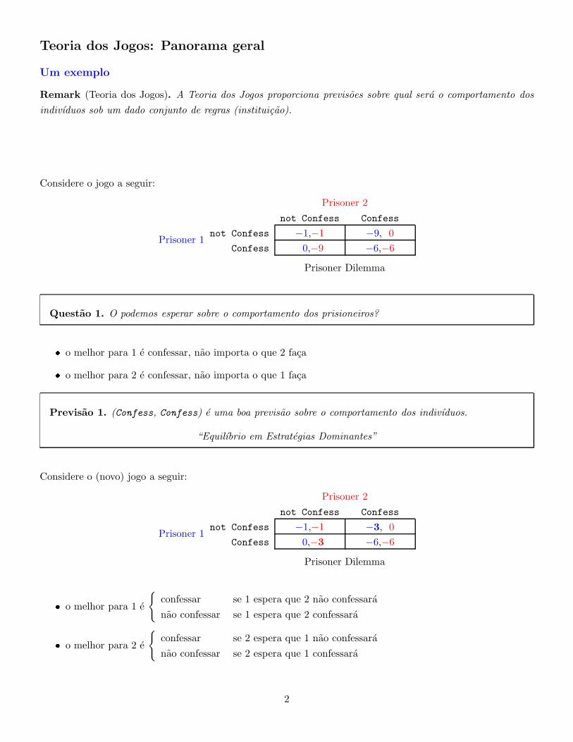
Considere o jogo a seguir:
Prisoner 1
Prisoner 2
not Confess Confess
not Confess −1,−1 −9, 0
Confess 0,−9 −6,−6
Prisoner Dilemma
Questao 1. O podemos esperar sobre o comportamento dos prisioneiros?
� o melhor para 1 e confessar, nao importa o que 2 faca
� o melhor para 2 e confessar, nao importa o que 1 faca
Previsao 1. (Confess, Confess) e uma boa previsao sobre o comportamento dos indivıduos.
“Equilıbrio em Estrategias Dominantes”
Considere o (novo) jogo a seguir:
Prisoner 1
Prisoner 2
not Confess Confess
not Confess −1,−1 −3, 0
Confess 0,−3 −6,−6
Prisoner Dilemma
� o melhor para 1 e
{
confessar se 1 espera que 2 nao confessara
nao confessar se 1 espera que 2 confessara
� o melhor para 2 e
{
confessar se 2 espera que 1 nao confessara
nao confessar se 2 espera que 1 confessara
2
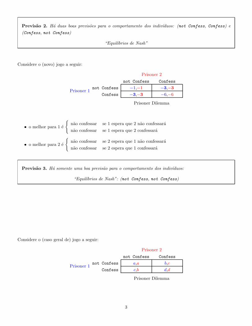
Previsao 2. Ha duas boas previsoes para o comportamento dos indivıduos: (not Confess, Confess) e
(Confess, not Confess)
“Equilıbrios de Nash”
Considere o (novo) jogo a seguir:
Prisoner 1
Prisoner 2
not Confess Confess
not Confess −1,−1 −3,−3
Confess −3,−3 −6,−6
Prisoner Dilemma
� o melhor para 1 e
{
nao confessar se 1 espera que 2 nao confessara
nao confessar se 1 espera que 2 confessara
� o melhor para 2 e
{
nao confessar se 2 espera que 1 nao confessara
nao confessar se 2 espera que 1 confessara
Previsao 3. Ha somente uma boa previsao para o comportamento dos indivıduos:
“Equilıbrios de Nash”: (not Confess, not Confess)
Considere o (caso geral de) jogo a seguir:
Prisoner 1
Prisoner 2
not Confess Confess
not Confess a,a b,c
Confess c,b d,d
Prisoner Dilemma
3
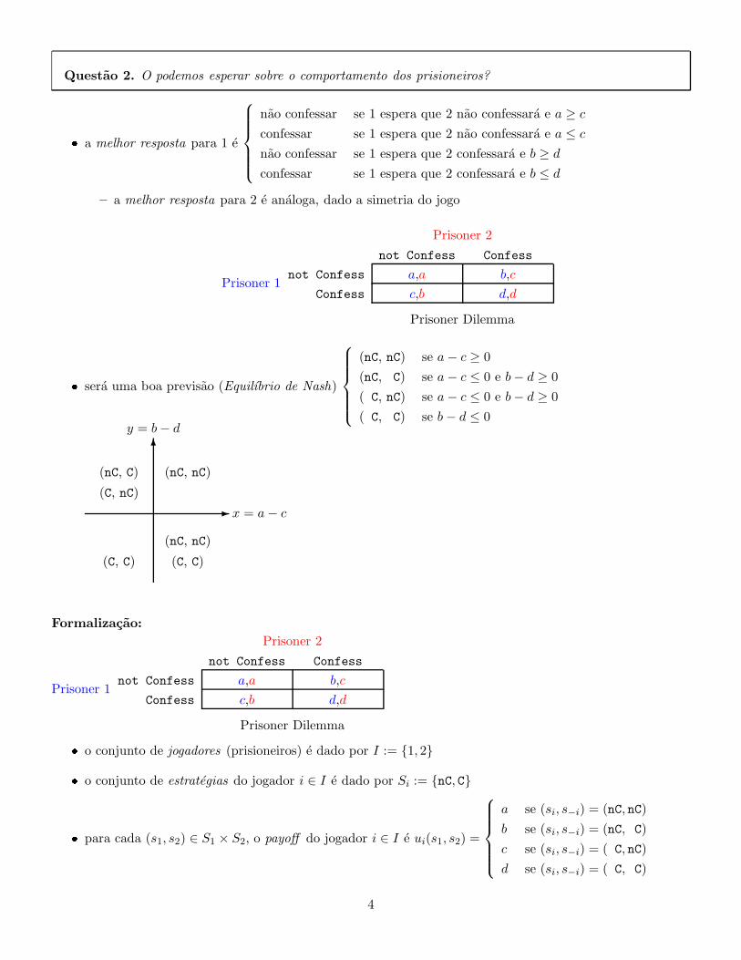
Questao 2. O podemos esperar sobre o comportamento dos prisioneiros?
� a melhor resposta para 1 e
nao confessar se 1 espera que 2 nao confessara e a ≥ c
confessar se 1 espera que 2 nao confessara e a ≤ c
nao confessar se 1 espera que 2 confessara e b ≥ d
confessar se 1 espera que 2 confessara e b ≤ d
– a melhor resposta para 2 e analoga, dado a simetria do jogo
Prisoner 1
Prisoner 2
not Confess Confess
not Confess a,a b,c
Confess c,b d,d
Prisoner Dilemma
� sera uma boa previsao (Equilıbrio de Nash)
(nC, nC) se a− c ≥ 0
(nC, C) se a− c ≤ 0 e b− d ≥ 0
( C, nC) se a− c ≤ 0 e b− d ≥ 0
( C, C) se b− d ≤ 0
✲
✻
x = a− c
y = b− d
(nC, nC)
(nC, nC)
(C, C)(C, C)
(nC, C)
(C, nC)
Formalizacao:
Prisoner 1
Prisoner 2
not Confess Confess
not Confess a,a b,c
Confess c,b d,d
Prisoner Dilemma
� o conjunto de jogadores (prisioneiros) e dado por I := {1, 2}
� o conjunto de estrategias do jogador i ∈ I e dado por Si := {nC, C}
� para cada (s1, s2) ∈ S1 × S2, o payoff do jogador i ∈ I e ui(s1, s2) =
a se (si, s−i) = (nC, nC)
b se (si, s−i) = (nC, C)
c se (si, s−i) = ( C, nC)
d se (si, s−i) = ( C, C)
4
� o conjunto de melhores respostas de i para a conjectura s−i e dado por
Ri(s−i) := argmaxσ∈Si
ui(σ, s−i)
Definicao 1. O perfil de estrategias (s1, s2) e um equilıbrio de Nash se s1 ∈ R1(s2) e s2 ∈ R2(s1). Ou
seja, se si e ponto fixo de Ri ◦R−i:
s1 ∈ R1(R2(s1)) e s2 ∈ R2(R1(s2))
Teorema 1 (Nash et al. (1950)). In the n-player normal-form game
G = {S1, S2, · · · , Sn;u1, u2, · · · , un},
� if n is finite and Si is finite for every i
then there is at least one Nash Equilibrium (possibly involving mixed strategies).
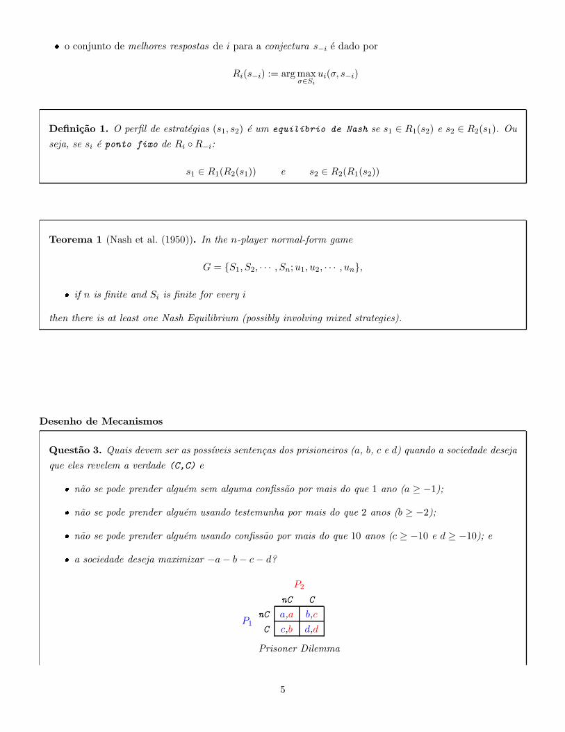
Desenho de Mecanismos
Questao 3. Quais devem ser as possıveis sentencas dos prisioneiros (a, b, c e d) quando a sociedade deseja
que eles revelem a verdade (C,C) e
� nao se pode prender alguem sem alguma confissao por mais do que 1 ano (a ≥ −1);
� nao se pode prender alguem usando testemunha por mais do que 2 anos (b ≥ −2);
� nao se pode prender alguem usando confissao por mais do que 10 anos (c ≥ −10 e d ≥ −10); e
� a sociedade deseja maximizar −a− b− c− d?
P1
P2
nC C
nC a,a b,c
C c,b d,d
Prisoner Dilemma
5
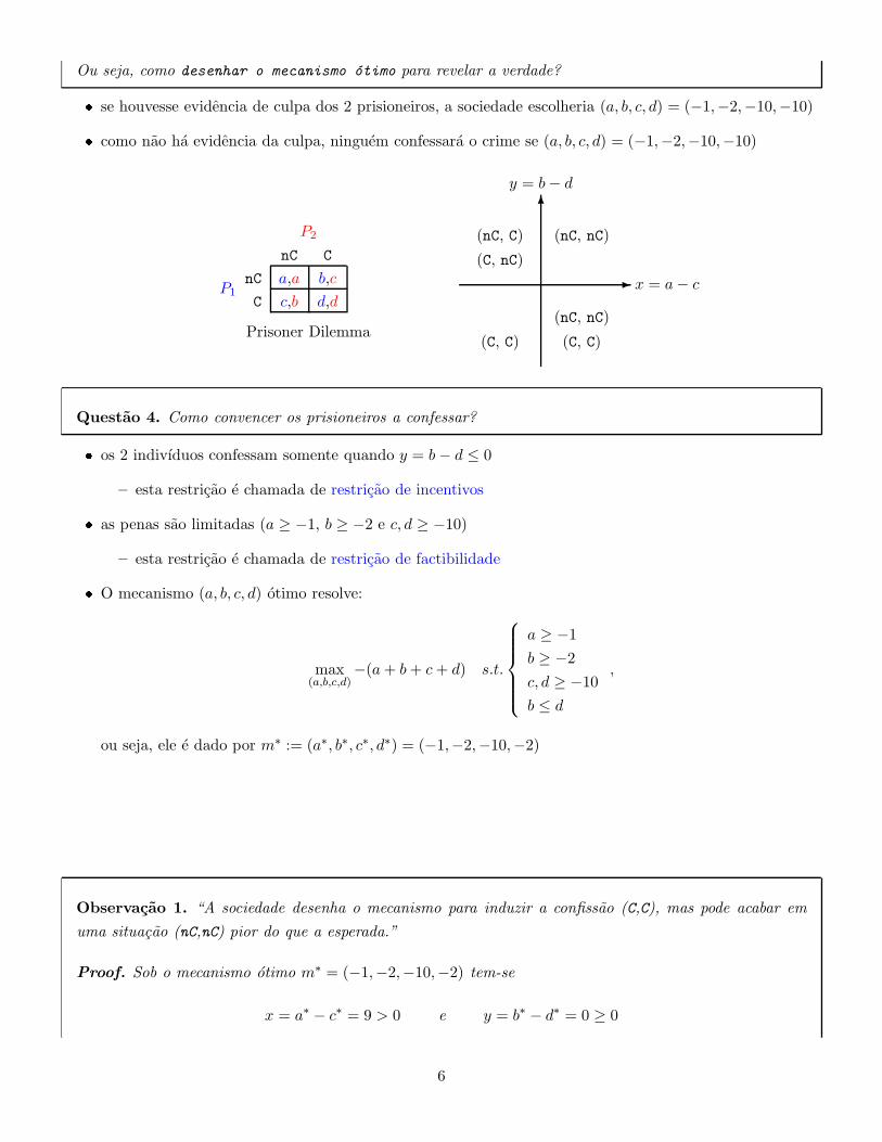
Ou seja, como desenhar o mecanismo otimo para revelar a verdade?
� se houvesse evidencia de culpa dos 2 prisioneiros, a sociedade escolheria (a, b, c, d) = (−1,−2,−10,−10)
� como nao ha evidencia da culpa, ninguem confessara o crime se (a, b, c, d) = (−1,−2,−10,−10)
P1
P2
nC C
nC a,a b,c
C c,b d,d
Prisoner Dilemma
✲
✻
x = a− c
y = b− d
(nC, nC)
(nC, nC)
(C, C)(C, C)
(nC, C)
(C, nC)
Questao 4. Como convencer os prisioneiros a confessar?
� os 2 indivıduos confessam somente quando y = b− d ≤ 0
– esta restricao e chamada de restricao de incentivos
� as penas sao limitadas (a ≥ −1, b ≥ −2 e c, d ≥ −10)
– esta restricao e chamada de restricao de factibilidade
� O mecanismo (a, b, c, d) otimo resolve:
max(a,b,c,d)
−(a+ b+ c+ d) s.t.
a ≥ −1
b ≥ −2
c, d ≥ −10
b ≤ d
,
ou seja, ele e dado por m∗ := (a∗, b∗, c∗, d∗) = (−1,−2,−10,−2)
Observacao 1. “A sociedade desenha o mecanismo para induzir a confissao (C,C), mas pode acabar em
uma situacao (nC,nC) pior do que a esperada.”
Proof. Sob o mecanismo otimo m∗ = (−1,−2,−10,−2) tem-se
x = a∗ − c∗ = 9 > 0 e y = b∗ − d∗ = 0 ≥ 0
6
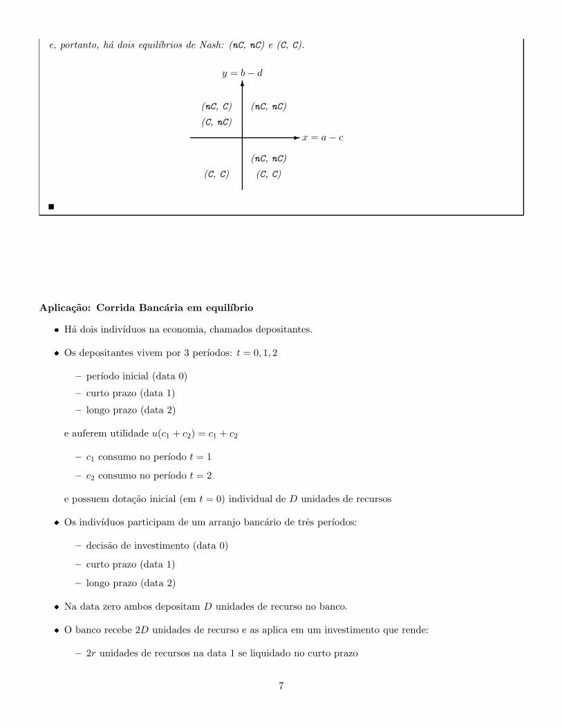
e, portanto, ha dois equilıbrios de Nash: (nC, nC) e (C, C).
✲
✻
x = a− c
y = b− d
(nC, nC)
(nC, nC)
(C, C)(C, C)
(nC, C)
(C, nC)
Aplicacao: Corrida Bancaria em equilıbrio
� Ha dois indivıduos na economia, chamados depositantes.
� Os depositantes vivem por 3 perıodos: t = 0, 1, 2
– perıodo inicial (data 0)
– curto prazo (data 1)
– longo prazo (data 2)
e auferem utilidade u(c1 + c2) = c1 + c2
– c1 consumo no perıodo t = 1
– c2 consumo no perıodo t = 2
e possuem dotacao inicial (em t = 0) individual de D unidades de recursos
� Os indivıduos participam de um arranjo bancario de tres perıodos:
– decisao de investimento (data 0)
– curto prazo (data 1)
– longo prazo (data 2)
� Na data zero ambos depositam D unidades de recurso no banco.
� O banco recebe 2D unidades de recurso e as aplica em um investimento que rende:
– 2r unidades de recursos na data 1 se liquidado no curto prazo
7
– 2R unidades de recursos na data 2 se liquidado no longo prazo
� Se ambos os depositantes sacam recursos na data 1,
– o investimento e liquidado no curto prazo
– cada depositante recebe r
� Se somente um dos depositantes saca recursos na data 1,
– o investimento e liquidado no curto prazo
– o depositante que saca na data 1 recebe D
– o depositante que saca na data 2 recebe 2r −D
� Se ambos os depositantes sacam recursos na data 2,
– o investimento e liquidado somente no longo prazo
– cada depositante recebe R
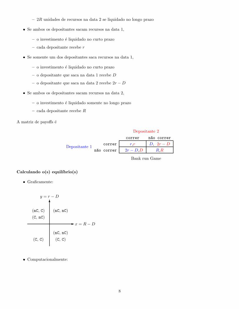
A matriz de payoffs e
Depositante 1
Depositante 2
correr n~ao correr
correr r,r D, 2r −D
n~ao correr 2r −D,D R,R
Bank run Game
Calculando o(s) equilıbrio(s)
� Graficamente:
✲
✻
x = R−D
y = r −D
(nC, nC)
(nC, nC)
(C, C)(C, C)
(nC, C)
(C, nC)
� Computacionalmente:
8
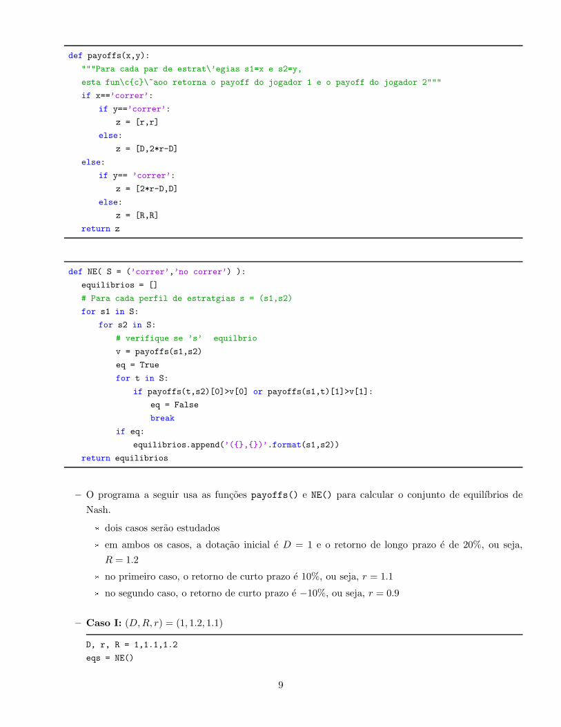
def payoffs(x,y):
"""Para cada par de estrat\’egias s1=x e s2=y,
esta fun\c{c}\~aoo retorna o payoff do jogador 1 e o payoff do jogador 2"""
if x==’correr’:
if y==’correr’:
z = [r,r]
else:
z = [D,2*r-D]
else:
if y== ’correr’:
z = [2*r-D,D]
else:
z = [R,R]
return z
def NE( S = (’correr’,’no correr’) ):
equilibrios = []
# Para cada perfil de estratgias s = (s1,s2)
for s1 in S:
for s2 in S:
# verifique se ’s’ equilbrio
v = payoffs(s1,s2)
eq = True
for t in S:
if payoffs(t,s2)[0]>v[0] or payoffs(s1,t)[1]>v[1]:
eq = False
break
if eq:
equilibrios.append(’({},{})’.format(s1,s2))
return equilibrios
– O programa a seguir usa as funcoes payoffs() e NE() para calcular o conjunto de equilıbrios de
Nash.
* dois casos serao estudados
* em ambos os casos, a dotacao inicial e D = 1 e o retorno de longo prazo e de 20%, ou seja,
R = 1.2
* no primeiro caso, o retorno de curto prazo e 10%, ou seja, r = 1.1
* no segundo caso, o retorno de curto prazo e −10%, ou seja, r = 0.9
– Caso I: (D,R, r) = (1, 1.2, 1.1)
D, r, R = 1,1.1,1.2
eqs = NE()
9
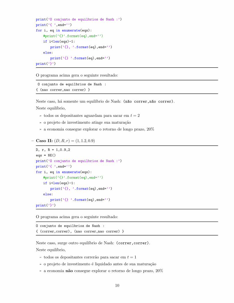
print(’O conjunto de equilbrios de Nash :’)
print(’{ ’,end=’’)
for i, eq in enumerate(eqs):
#print(’{}’.format(eq),end=’’)
if i<len(eqs)-1:
print(’{}, ’.format(eq),end=’’)
else:
print(’{} ’.format(eq),end=’’)
print(’}’)
O programa acima gera o seguinte resultado:
O conjunto de equilbrios de Nash :
{ (nao correr,nao correr) }
Neste caso, ha somente um equilıbrio de Nash: (n~ao correr,n~ao correr).
Neste equilıbrio,
* todos os depositantes aguardam para sacar em t = 2
* o projeto de investimento atinge sua maturacao
* a economia consegue explorar o retorno de longo prazo, 20%
– Caso II: (D,R, r) = (1, 1.2, 0.9)
D, r, R = 1,0.9,2
eqs = NE()
print(’O conjunto de equilbrios de Nash :’)
print(’{ ’,end=’’)
for i, eq in enumerate(eqs):
#print(’{}’.format(eq),end=’’)
if i<len(eqs)-1:
print(’{}, ’.format(eq),end=’’)
else:
print(’{} ’.format(eq),end=’’)
print(’}’)
O programa acima gera o seguinte resultado:
O conjunto de equilbrios de Nash :
{ (correr,correr), (nao correr,nao correr) }
Neste caso, surge outro equilıbrio de Nash: (correr,correr).
Neste equilıbrio,
* todos os depositantes correrao para sacar em t = 1
* o projeto de investimento e liquidado antes de sua maturacao
* a economia nao consegue explorar o retorno de longo prazo, 20%
10
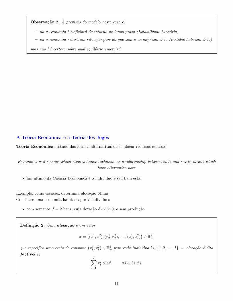
Observacao 2. A previsao do modelo neste caso e:
– ou a economia beneficiara do retorno de longo prazo (Estabilidade bancaria)
– ou a economia estara em situacao pior do que sem o arranjo bancario (Instabilidade bancaria)
mas nao ha certeza sobre qual equilıbrio emergira.
A Teoria Economica e a Teoria dos Jogos
Teoria Economica: estudo das formas alternativas de se alocar recursos escassos.
Economics is a science which studies human behavior as a relationship between ends and scarce means which
have alternative uses
� fim ultimo da Ciencia Economica e o indivıduo e seu bem estar
Exemplo: como escassez determina alocacao otima
Considere uma economia habitada por I indivıduos
� com somente J = 2 bens, cuja dotacao e ωj ≥ 0, e sem producao
Definicao 2. Uma alocacao e um vetor
x =((x11, x
21), (x
12, x
22), . . . , (x
1I , x
2I))∈ R
2I+
que especifica uma cesta de consumo (x1i , x2i ) ∈ R
2+ para cada indivıduo i ∈ {1, 2, . . . , I}. A alocacao e dita
factıvel seI∑
i=1
xji ≤ ωj, ∀j ∈ {1, 2}.
11
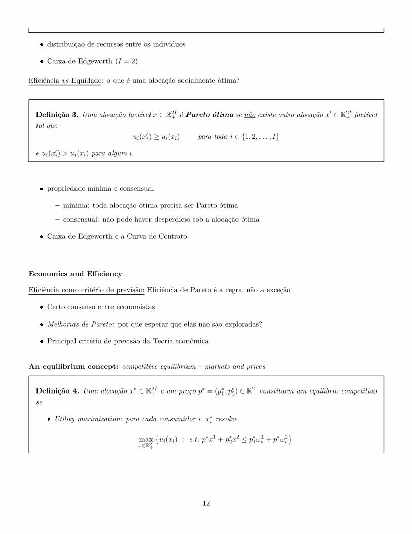
� distribuicao de recursos entre os indivıduos
� Caixa de Edgeworth (I = 2)
Eficiencia vs Equidade: o que e uma alocacao socialmente otima?
Definicao 3. Uma alocacao factıvel x ∈ R2I+ e Pareto otima se nao existe outra alocacao x′ ∈ R
2I+ factıvel
tal que
ui(x′i) ≥ ui(xi) para todo i ∈ {1, 2, . . . , I}
e ui(x′i) > ui(xi) para algum i.
� propriedade mınima e consensual
– mınima: toda alocacao otima precisa ser Pareto otima
– consensual: nao pode haver desperdıcio sob a alocacao otima
� Caixa de Edgeworth e a Curva de Contrato
Economics and Efficiency
Eficiencia como criterio de previsao: Eficiencia de Pareto e a regra, nao a excecao
� Certo consenso entre economistas
� Melhorias de Pareto: por que esperar que elas nao sao exploradas?
� Principal criterio de previsao da Teoria economica
An equilibrium concept: competitive equilibrium – markets and prices
Definicao 4. Uma alocacao x∗ ∈ R2I+ e um preco p∗ = (p∗1, p
∗2) ∈ R
2+ constituem um equilıbrio competitivo
se
� Utility maximization: para cada consumidor i, x∗i resolve
maxx∈R2
+
{ui(xi) : s.t. p∗1x
1 + p∗2x2 ≤ p∗1ω
1i + p∗ω2
i
}
12
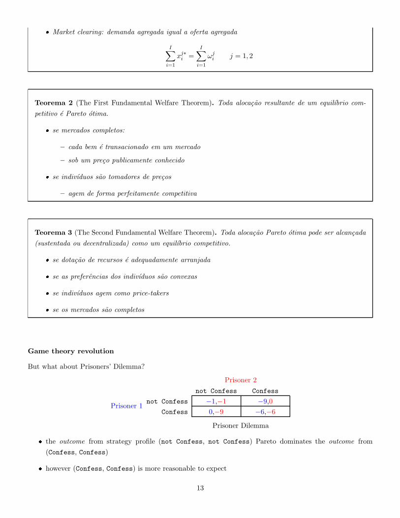
� Market clearing: demanda agregada igual a oferta agregada
I∑
i=1
xj∗i =I∑
i=1
ωji j = 1, 2
Teorema 2 (The First Fundamental Welfare Theorem). Toda alocacao resultante de um equilıbrio com-
petitivo e Pareto otima.
� se mercados completos:
– cada bem e transacionado em um mercado
– sob um preco publicamente conhecido
� se indivıduos sao tomadores de precos
– agem de forma perfeitamente competitiva
Teorema 3 (The Second Fundamental Welfare Theorem). Toda alocacao Pareto otima pode ser alcancada
(sustentada ou decentralizada) como um equilıbrio competitivo.
� se dotacao de recursos e adequadamente arranjada
� se as preferencias dos indivıduos sao convexas
� se indivıduos agem como price-takers
� se os mercados sao completos
Game theory revolution
But what about Prisoners’ Dilemma?
Prisoner 1
Prisoner 2
not Confess Confess
not Confess −1,−1 −9,0
Confess 0,−9 −6,−6
Prisoner Dilemma
� the outcome from strategy profile (not Confess, not Confess) Pareto dominates the outcome from
(Confess, Confess)
� however (Confess, Confess) is more reasonable to expect
13
Another equilibrium concept: Nash equilibrium
Strategic interdependence:
� Each individual’s welfare depends not only on his own actions but also on the actions of the other
individuals
� The actions that are best for an individual to take may depend on what he expects the other players to
do
Even more equilibrium concepts and some refinements:
� Equilibrium in Dominant strategies
� Nash equilibrium
� subgame-Perfect Nash equilibrium
� Bayesian Nash equilibrium
� Perfect Bayesian Nash equilibrium
� The Intuitive Criterion (Cho and Kreps (1987))
Mechanism Design
Questao 5 (Choosing among games:). How to design games in order to implement optimal allocations?
� Principal-Agent problems
– moral hazard
– adverse selection
� The Social Planner problems (social optimum)
– fiscal policy
– monetary policy
– regulation
� The Revelation Principle
14
Cap. 1 - Static Games of Complete Information
Static Games of Complete Information:
� Static:
– players simultaneously choose actions
– payoffs players receive depend on the combination of actions just chosen
� Complete information:
– each player’s payoff function is common knowledge among all players
– exemplo: leiloes
Questao 6. What is a game?
Definicao 5. A game is a formal representation of a situation in which a number of individuals interact
in a setting of strategic interdependence.
� Each individual’s welfare depends not only on his own actions but also on the actions of the other
individuals
� The actions that are best for an individual to take may depend on what he expects the other players to
do
1.1 Normal form games and Nash equilibrium
Normal-form representation of games
In the normal-form representation of the game
� each player simultaneously chooses a strategy.
� the combination of strategies chosen by players determines a payoff for each player
Exemplo 1 (The prisoners’ dilemma).
The environment
� Two suspects are arrested and charged with a crime
� The police lack sufficient evidence to convict the suspects, unless at least one confesses
� The suspects are in separate cells
� The police explain the consequences that will follow from the actions they could take
15

Actions and payoffs
� If neither confesses, they will be convicted of a minor offense and sentenced to one month in jail
� If both confess then both will be sentenced to jail for six months
� If one confesses but the other does not, then the confessor will be released immediately but the other
will be sentenced to nine months in jail
– Six for crime
– Three for obstructing justice
Matrix representation
� Each player has 2 strategies: Confess or not Confess
� Implicitly assumed that each player does not like to stay in jail
Prisoner 1
Prisoner 2
not Confess Confess
not Confess −1,−1 −9,0
Confess 0,−9 −6,−6
Prisoner Dilemma
General case:
The normal form representation
(a) Players
(b) Strategies
(c) Payoffs
Players: A finite set I of players
� We write “player i” where i is the name of the player and I is the collection of names
� We denote by n the number of players, i.e., n = #I
� The set I may be denoted by I = {1, 2, · · · , n}
Strategies: The set of strategies available to player i is denoted by Si
� An element si ∈ Si is called a strategy (play or action)
� The set Si is called strategy space and may have any structure: finite, countable, metric space, vector
space
� The collection (si)i∈I = (s1, · · · , sn) is called a strategy profile and denoted by s or s
16
� Given an agent j and a profile s, we denote by (s−j ; s′j) the new profile σ = (σi)i∈I defined by
σi =
{
s′j if i = j
si if i 6= j
1 < j < n ⇒ (s−j; s′j) = (s1, . . . , sj−1, s
′j , sj+1, . . . , sn)
Payoffs:
� The payoff of player i is a function
ui :
∏
j∈I Sj → [−∞,+∞]
s 7→ ui(s)
where ui(s) is the payoff of player i when
– he plays strategy si
– and any other player j plays strategy sj
� We use alternatively the following notation
ui(s) = ui ((sj)j∈I) = ui(s−i; si) = ui(s1, s2, . . . , sn)
Definicao 6. A game in normal form is a family
G = (Si, ui)i∈I
where for each i ∈ I
� Si is a set
� ui is a function from S =∏
j∈I Sj to [−∞,+∞]
Observacao 3. We should know describe how to solve a game-theoretic problem
Questao 7. Can we anticipate how a game will be played?
� What should we expect to observe in a game played by
– rational players
17
– who are fully knowledgeable about
* the structure of the game
* and each others’ rationality?
Simultaneous moves: In a normal form game the players choose their strategies simultaneously
� This does not imply that they act simultaneously
� It suffices that each choose his or her action without knowledge of the others’ choices
– Prisoners’ dilemma: the prisoners may reach decisions at arbitrary times but it must be in separate
cells
– Bidders in an sealed-bid auction
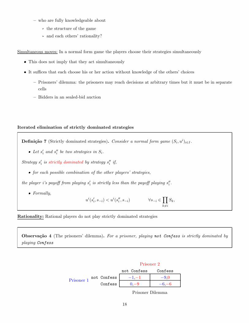
Iterated elimination of strictly dominated strategies
Definicao 7 (Strictly dominated strategies). Consider a normal form game (Si, ui)i∈I .
� Let s′i and s′′i be two strategies in Si.
Strategy s′i is strictly dominated by strategy s′′i if,
� for each possible combination of the other players’ strategies,
the player i’s payoff from playing s′i is strictly less than the payoff playing s′′i .
� Formally,
ui(s′i, s−i) < ui(s′′i , s−i) ∀s−i ∈∏
k 6=i
Sk,
Rationality: Rational players do not play strictly dominated strategies
Observacao 4 (The prisoners’ dilemma). For a prisoner, playing not Confess is strictly dominated by
playing Confess
Prisoner 1
Prisoner 2
not Confess Confess
not Confess −1,−1 −9,0
Confess 0,−9 −6,−6
Prisoner Dilemma
18

Assume we are player 1
� If player 2 chooses Confess
– We prefer to play Confess and stay 6 months in jail
– rather than playing not Confess and stay 9 months in jail
� If player 2 chooses not Confess
– We prefer to play Confess and be free
– rather than playing not Confess and stay 1 month in jail
� A rational player will not choose to play not Confess
– therefore, a rational player will choose to play Confess
The outcome reached by the two prisoners is (Confess,Confess)
� This results in a worse payoff for both players than would
(Not Confess,Not confess)
– This inefficiency is a consequence of the lack of coordination
� This happens in many other situations
– the arms race
– the free-rider problem in the provision of public goods
Iterated elimination
Questao 8. Can we use the idea that “rational players do not play strictly dominated strategies” to find a
solution to other games?
� Consider a game (in normal form) with two players
I = {1, 2}
� Player 1 has two available strategies
S1 = {Up;Down}
� Player 2 has three available strategies
S2 = {Left;Middle;Right}
� The payoffs are given by the following matrix
Player 1
Player 2
Left Middle Right
Up 1, 0 1, 2 0, 1
Down 0, 3 0, 1 2, 0
19

� for Player 1
– Up is not strictly dominated by Down
– Down is not strictly dominated by Up
� for Player 2
– Right is strictly dominated by Middle
– player 2 will never play Right
� if Player 1 knows that Player 2 is rational
– then Player 1 can eliminate Right from Player 2’s strategy set
� then both players can play the game as if it were the following game
Player 1
Player 2
Left Middle
Up 1, 0 1, 2
Down 0, 3 0, 1
� For Player 1 the strategy Down is strictly dominated by Up
� If Player 2 knows that
– Player 1 is rational; and
– Player 1 knows that Player 2 is rational
then Player 2 can eliminate Down from S1
� Now the game is as follows
Player 1
Player 2
Left Middle
Up 1, 0 1, 2
� For Player 2 the strategy Left is strictly dominated by Middle
Observacao 5. By iterated elimination of strictly dominated strategies
� the outcome of the game is (Up,Middle)
Definicao 8 (Iterated elimination of strictly dominated strategies). This process is called iterated elimi-
nation of strictly dominated strategies.
20

Proposicao 1. The set of strategy profiles that survive to iterated elimination of strictly dominated strate-
gies is independent of the order of deletion
Drawbacks:
(i) Each step requires a further assumption about what the players know about each other’s rationality
� to apply the process for an arbitrary number of steps,
we need to assume that
it is common knowledge that players are rational
Definicao 9. Players’ rationality is common knowledge if
– All the players are rational
– All the players know that all the players are rational
– So on, ad infinitum
(ii) this process often produces a very imprecise prediction about the play of the game
Consider the following game
L C R
U 0, 4 4, 0 5, 3
M 4, 0 0, 4 5, 3
D 3, 5 3, 5 6, 6
� There are no strictly dominated strategies to be eliminated
� The process produces no prediction whatsoever about the play of the game
Questao 9. Is there a stronger solution concept than IESDS which produces much tighter predictions in a
very broad class of games?
Nash equilibrium: motivation and definition
Motivation:
Suppose that game theory makes a unique prediction about the strategy each player will choose
� in order for this prediction to be compatible with incentives (or correct) it is necessary that
– each player be willing to choose the strategy predicted by the theory
21
– each player’s predicted strategies must be that player’s best response to the predicted strategies of
other players
� such a prediction could be called
strategically stable or self-enforcing
– no single player wants to deviate from his or her predicted strategy
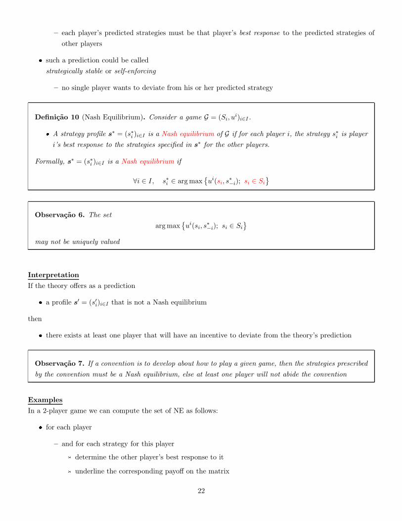
Definicao 10 (Nash Equilibrium). Consider a game G = (Si, ui)i∈I .
� A strategy profile s∗ = (s∗i )i∈I is a Nash equilibrium of G if for each player i, the strategy s∗i is player
i’s best response to the strategies specified in s∗ for the other players.
Formally, s∗ = (s∗i )i∈I is a Nash equilibrium if
∀i ∈ I, s∗i ∈ argmax{ui(si, s
∗−i); si ∈ Si
}
Observacao 6. The set
argmax{ui(si, s
∗−i); si ∈ Si
}
may not be uniquely valued
Interpretation
If the theory offers as a prediction
� a profile s′ = (s′i)i∈I that is not a Nash equilibrium
then
� there exists at least one player that will have an incentive to deviate from the theory’s prediction
Observacao 7. If a convention is to develop about how to play a given game, then the strategies prescribed
by the convention must be a Nash equilibrium, else at least one player will not abide the convention
Examples
In a 2-player game we can compute the set of NE as follows:
� for each player
– and for each strategy for this player
* determine the other player’s best response to it
* underline the corresponding payoff on the matrix
22
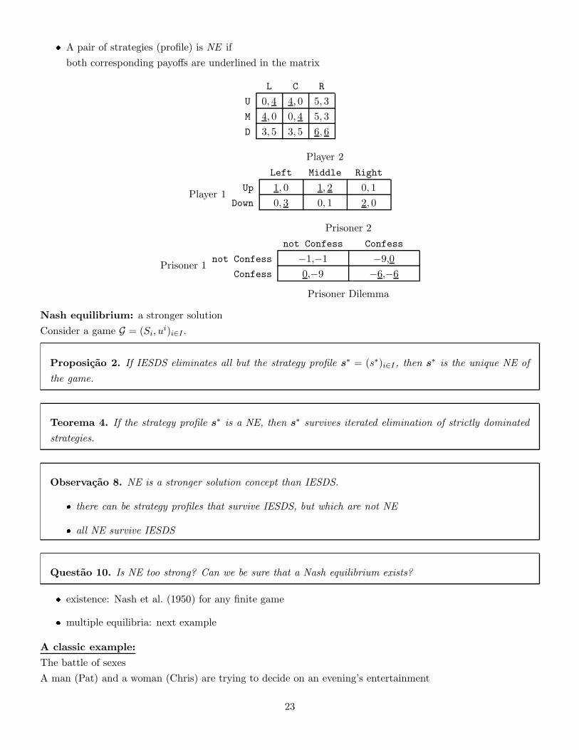
� A pair of strategies (profile) is NE if
both corresponding payoffs are underlined in the matrix
L C R
U 0, 4 4, 0 5, 3
M 4, 0 0, 4 5, 3
D 3, 5 3, 5 6, 6
Player 1
Player 2
Left Middle Right
Up 1, 0 1, 2 0, 1
Down 0, 3 0, 1 2, 0
Prisoner 1
Prisoner 2
not Confess Confess
not Confess −1,−1 −9,0
Confess 0,−9 −6,−6
Prisoner Dilemma
Nash equilibrium: a stronger solution
Consider a game G = (Si, ui)i∈I .
Proposicao 2. If IESDS eliminates all but the strategy profile s∗ = (s∗)i∈I , then s∗ is the unique NE of
the game.
Teorema 4. If the strategy profile s∗ is a NE, then s∗ survives iterated elimination of strictly dominated
strategies.
Observacao 8. NE is a stronger solution concept than IESDS.
� there can be strategy profiles that survive IESDS, but which are not NE
� all NE survive IESDS
Questao 10. Is NE too strong? Can we be sure that a Nash equilibrium exists?
� existence: Nash et al. (1950) for any finite game
� multiple equilibria: next example
A classic example:
The battle of sexes
A man (Pat) and a woman (Chris) are trying to decide on an evening’s entertainment
23
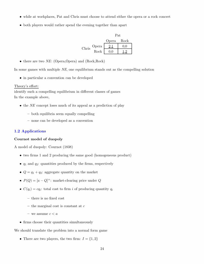
� while at workplaces, Pat and Chris must choose to attend either the opera or a rock concert
� both players would rather spend the evening together than apart
Chris
Pat
Opera Rock
Opera 2,1 0,0
Rock 0,0 1,2
� there are two NE : (Opera,Opera) and (Rock,Rock)
In some games with multiple NE, one equilibrium stands out as the compelling solution
� in particular a convention can be developed
Theory’s effort:
identify such a compelling equilibrium in different classes of games
In the example above,
� the NE concept loses much of its appeal as a prediction of play
– both equilibria seem equally compelling
– none can be developed as a convention
1.2 Applications
Cournot model of duopoly
A model of duopoly: Cournot (1838)
� two firms 1 and 2 producing the same good (homogeneous product)
� q1 and q2: quantities produced by the firms, respectively
� Q = q1 + q2: aggregate quantity on the market
� P (Q) = [a−Q]+: market-clearing price under Q
� C(qi) = cqi: total cost to firm i of producing quantity qi
– there is no fixed cost
– the marginal cost is constant at c
– we assume c < a
� firms choose their quantities simultaneously
We should translate the problem into a normal form game
� There are two players, the two firm: I = {1, 2}
24
� The strategies available to each firm are the different quantities Qi = [0,∞)
� An element of Qi is denoted qi
– One could reduce the set Qi to [0, a] since P (Q) = 0 for Q ≥ a
� The payoff of firm i for a profile (qi, qj) is its profit defined by
πi(qi, qj) = qi[P (qi + qj)− c] = qi([a− (qi + qj)]
+ − c)
The game is then G = (Qi, πi)i∈I
Nash equilibrium (NE)
A strategy to find a NE is to look for necessary condition (and then to check that it is sufficient)
� if (q∗1 , q∗2) is a Nash equilibrium, then
∀i ∈ I, q∗i ∈ argmax{πi(qi; q∗j ) : qi ≥ 0}
� we have
πi(qi; q∗j ) =
{
qi[(a− c− q∗j )− qi] if qi < a− q∗j−qic if qi ≥ a− q∗j
� all strategies qi ≥ a− q∗j are SD by qi = 0. Therefore,
q∗i ∈ argmax{πi(qi; q∗j ) : 0 ≤ qi < a− q∗j}
and the first order condition is necessary and sufficient
� objective function’s derivative is∂πi∂qi
(qi, q∗j ) = a− c− q∗j − 2qi
� assuming that q∗i ∈ (0, a− c) for each firm i, we have
q∗i =1
2(a− q∗j − c)
which yields
q∗i =a− c
3, ∀i ∈ I
obs.: this is consistent with the assumption q∗i ∈ (0, a − c)
Observacao 9. There is a unique Nash equilibrium, called Cournot equilibrium
Interpretation
Each firm would like to be a monopolist in this market
25
� it would choose qi to maximize πi(qi, 0). The solution is
qm =a− c
2
and the associated profit is
πi(qm; 0) =(a− c)2
4
With the two firms
� aggregate profits would be maximized by setting
q1 + q2 = qm
this would occur with qi = qm/2
Problem with the strategy profile (qm/2, qm/2):
� the market price P (qm) is too high
– at this price, each firm has an incentive to deviate by increasing the production
– in spite of the fact that such a deviation drives down the market price, the profit obtained still
increases
In the Cournot equilibrium,
� the aggregate quantity is higher
� so the associated price is lower
the temptation to increase output is reduced,
� just enough that each firm i is just deterred from increasing qi
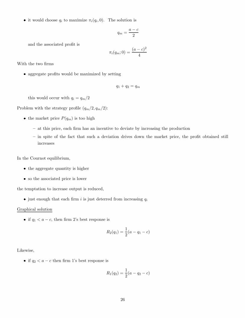
Graphical solution
� if q1 < a− c, then firm 2’s best response is
R2(q1) =1
2(a− q1 − c)
Likewise,
� if q2 < a− c then firm 1’s best response is
R1(q2) =1
2(a− q2 − c)
26
� The two best response functions intersect only once,
at the equilibrium profile (q∗1 , q∗2)
Cournot duopoly and iterated elimination
A third proof: iterated elimination of strictly dominated strategies
� if there is a unique solution then it is a Nash equilibrium
Proposicao 3. The monopoly quantity qm = a−c2 strictly dominates any higher quantity.
We can then consider the game G(3) = (Q(3)i , πi)i∈I with
Q(3)i = [0, qm]
Proof. Step 1: Assume qm + qj < a. Then
πi(qm; qj) = qm
[a− c
2− qj
]
while
πi(qm + x, qj) = [qm + x]
[a− c
2− x− qj
]
= πi(qm, qj)− x(x+ qj)
Step 2: Assume qm + qj > a. Then,
πi(qm + x; qj) = −c[qm + x]
27
Proposicao 4. Given that quantities exceeding qm = (a − c)/2 have been eliminated, the quantity qm/2
strictly dominates any lower quantity.
Formally,
� for any x ∈ (0, qm/2] we have
πi[qm/2, qj ] > πi[qm/2 − x, qj ]; ∀qj ∈ [0, (a − c)/2]
Proof.
πi(qm/2, qj) = qm/2
[3
4(a− c)− qj
]
and
πi(qm/2− x, qj) = [qm/2− x]
[3
4(a− c) + x− qj
]
= πi(qm/2, qj)− x
[a− c
2+ x− qj
]
After these two steps, the quantities remaining in each firm’s strategy space are those in the interval
[a− c
4,a− c
2
]
� repeating these arguments leads to ever smaller intervals of remaining quantities
� in the limit (we need countably many steps), these intervals converge to the single point q∗i = a−c3
Cournot duopoly and iterated elimination
If we add one or more firms in Cournot’s model
� then the first step of elimination continues to hold
� but that’s it
Observacao 10. IESDS yields only the imprecise prediction that each firm’s quantity will not exceed the
monopoly quantity
Example: Three firms
28
� Q−i: sum of the quantities chosen by the firms other than i
πi(qi;Q−i) =
{
qi(a− qi −Q−i − c) if qi +Q−i < a
−cqi if qi +Q−i > a
� it is again true that qm strictly dominates any higher quantity
∀x > 0; πi(qm;Q−i) > πi(qm + x;Q−i); ∀Q−i > 0
Each firm reduces its strategy set to [0, qm], but
� no further strategies can be eliminated
Proposicao 5. No quantity qi ∈ [0, qm] is strictly dominated
Proof. For each qi ∈ [0, qm] there is a Q−i such that
qi ∈ argmax{πi(q′i, Q−i) : q′i ∈ [0, qm]}
In effect, we know that Q−i ∈ [0, 2qm] = [0, a− c]. Fix qi ∈ [0, qm] and recall that
πi(qi;Q−i) =
{
qi(a− qi −Q−i − c) if qi +Q−i < a
−cqi if qi +Q−i > a.
Then, the FOC is satisfied for qi and Q−i = a− c− 2qi.
Bertrand model of duopoly
We consider a different model of how two duopolists might interact
� Bertrand (1883) suggested that firms actually choose prices, rather than quantities as in Cournot’s model
We consider the case of differentiated products
� firms 1 and 2 choose prices p1 and p2, respectively
� the quantity that consumers demand from firm i’s product is
qi(pi, pj) = [a− pi + bpj]+ 0 < b < 2
� b reflects the extent to which
firm i’s product is a substitute for firm j’s product
29
Observacao 11. This is an unrealistic demand function
� demand for firm i’s product is positive
� even when firm i charges an arbitrarily high price,
provided firm j also charges a high enough price.
� there are no fixed costs of production
� marginal cost of production is constant at a value c ∈ (0, a)
The normal form game:
� the set of players is I = {1, 2}
� the strategy set Pi of player i is Pi = [0,∞)
� the payoff function corresponds to profits:
πi(pi, pj) = qi(pi, pj)[pi − c] = [a− pi + bpj ]+(pi − c)
The game is G = (Pi, πi)i∈I
Nash equilibrium:
the price pair (p∗1, p∗2) is a Nash equilibrium if,
� for each firm i the price p∗i solves
max0≤pi<∞
πi(pi, p∗j) = max
c<pi<a+bp∗j
[a− pi + bp∗j ][pi − c]
� objective function’s derivative is∂πi∂pi
(pi, p∗j) = a+ c+ bp∗j − 2pi
and, therefore, the solution to firm i’s optimization problem is
p∗i =1
2(a+ bp∗j + c)
If (p∗1, p∗2) is a Nash equilibrium, one must have
p∗1 =1
2(a+ bp∗2 + c) and p∗2 =
1
2(a+ bp∗1 + c)
30
� if b < 2 then the unique Nash equilibrium is
p∗1 = p∗2 =a+ c
2− b
Final-offer arbritation
Consider a firm and a union which dispute wages
(i) the firm and the union simultaneously make offers
� the firm offers the wage wf
� the union offers the wage wu
(ii) an arbitrator chooses one of the two offers as the settlement
� x: ideal settlement arbitrator would like to impose
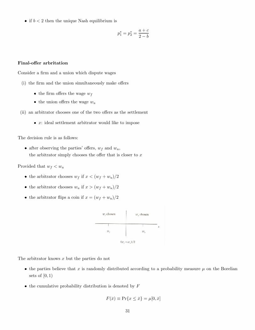
The decision rule is as follows:
� after observing the parties’ offers, wf and wu,
the arbitrator simply chooses the offer that is closer to x
Provided that wf < wu
� the arbitrator chooses wf if x < (wf + wu)/2
� the arbitrator chooses wu if x > (wf + wu)/2
� the arbitrator flips a coin if x = (wf + wu)/2
The arbitrator knows x but the parties do not
� the parties believe that x is randomly distributed according to a probability measure µ on the Borelian
sets of [0, 1)
� the cumulative probability distribution is denoted by F
F (x) ≡ Pr{x ≤ x} = µ[0, x]
31
� F : [0, 1) → [0, 1] is differentiable, with derivative f
� f represents the density function, i.e.,
∫
[0,∞)h(x)µ(dx) =
∫
[0,∞)h(x)f(x)dx
for every Borel measurable function h : [0,∞) → R+
Given the offers wf and wu, the parties believe that
� wf is chosen under probability
Pr{wf chosen} = µ
[
0,wf + wu
2
)
= F
(wf + wu
2
)
� wu is chosen under probability
Pr{wu chosen} = µ
[wf + wu
2,∞
)
= 1− F
(wf + wu
2
)
and, therefore, expected wage settlement is given by
E(w) = wf × Pr{wf chosen}+ wu × Pr{wu chosen}
= wfF
(wf +wu
2
)
+ wu
[
1− F
(wf + wu
2
)]
We assume that
� the firm wants to minimize E(w)
� the union wants to maximize E(w)
If (w∗f , w
∗u) is a Nash equilibrium, then
� w∗f must solve
min0≤wf<∞
{
wfF
(wf + w∗
u
2
)
+ w∗u
[
1− F
(wf + w∗
u
2
)]}
� w∗u must solve
max0≤wu<∞
{
w∗fF
(w∗f + wu
2
)
+ wu
[
1− F
(w∗f + wu
2
)]}
Suppose that (w∗f , w
∗u) is strictly positive
� FOC for the firm’s problem
(w∗u − w∗
f )×1
2f
(w∗u + w∗
f
2
)
= F
(w∗u + w∗
f
2
)
32
� FOC for the union’s problem
(w∗u − w∗
f )×1
2f
(w∗u +w∗
f
2
)
= 1− F
(w∗u + w∗
f
2
)
Therefore,
F
(w∗u + w∗
f
2
)
=1
2
The average of the offers must equal
� the median of the arbitrator’s preferred settlement
F
(w∗u + w∗
f
2
)
=1
2
The gap between the offers must equal
� the inverse of the value of the density function
� at the median of the arbitrator’s preferred settlement
w∗u − w∗
f =1
f(w∗
u+w∗
f
2
)
An example:
Suppose the arbitrator’s preferred settlement is normally distributed with mean m and variance σ2, i.e.,
f(x) =1√2πσ2
exp
{
− 1
2σ(x−m)2
}
� the median of the distribution equals the mean m
– the normal distribution is symmetric around its mean,
The necessary conditions are then translated into
w∗u + w∗
f
2= m and w∗
u − w∗f =
1
f(m)=
√2πσ2
The Nash equilibrium offers are
w∗u = m+
√
πσ2
2and w∗
f = m−√
πσ2
2
In equilibrium,
33
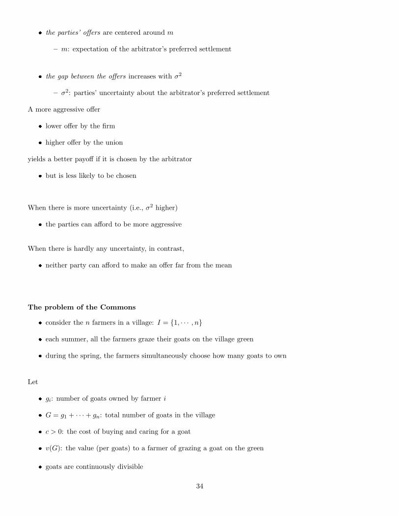
� the parties’ offers are centered around m
– m: expectation of the arbitrator’s preferred settlement
� the gap between the offers increases with σ2
– σ2: parties’ uncertainty about the arbitrator’s preferred settlement
A more aggressive offer
� lower offer by the firm
� higher offer by the union
yields a better payoff if it is chosen by the arbitrator
� but is less likely to be chosen
When there is more uncertainty (i.e., σ2 higher)
� the parties can afford to be more aggressive
When there is hardly any uncertainty, in contrast,
� neither party can afford to make an offer far from the mean
The problem of the Commons
� consider the n farmers in a village: I = {1, · · · , n}
� each summer, all the farmers graze their goats on the village green
� during the spring, the farmers simultaneously choose how many goats to own
Let
� gi: number of goats owned by farmer i
� G = g1 + · · ·+ gn: total number of goats in the village
� c > 0: the cost of buying and caring for a goat
� v(G): the value (per goats) to a farmer of grazing a goat on the green
� goats are continuously divisible
34
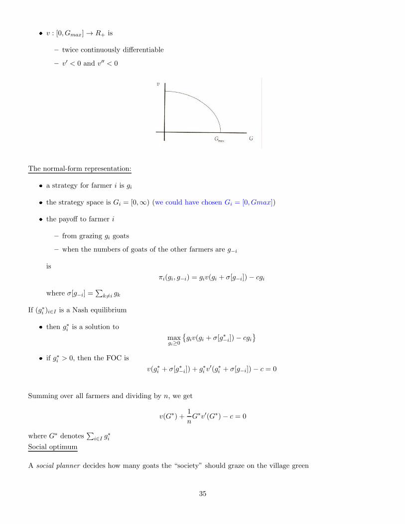
� v : [0, Gmax] → R+ is
– twice continuously differentiable
– v′ < 0 and v′′ < 0
The normal-form representation:
� a strategy for farmer i is gi
� the strategy space is Gi = [0,∞) (we could have chosen Gi = [0, Gmax])
� the payoff to farmer i
– from grazing gi goats
– when the numbers of goats of the other farmers are g−i
is
πi(gi, g−i) = giv(gi + σ[g−i])− cgi
where σ[g−i] =∑
k 6=i gk
If (g∗i )i∈I is a Nash equilibrium
� then g∗i is a solution to
maxgi≥0
{giv(gi + σ[g∗−i])− cgi
}
� if g∗i > 0, then the FOC is
v(g∗i + σ[g∗−i]) + g∗i v′(g∗i + σ[g−i])− c = 0
Summing over all farmers and dividing by n, we get
v(G∗) +1
nG∗v′(G∗)− c = 0
where G∗ denotes∑
i∈I g∗i
Social optimum
A social planner decides how many goats the “society” should graze on the village green
35
� the planner should solve
maxG≥0
{Gv(G) −Gc}
independent on the way the social profit should be divided
� the FOC is
v(Gs) +Gsv′(Gs)− c = 0
Lema 1. One must have G∗ > Gs.
Observacao 12. Too many goats are grazed in the Nash equilibrium, compared to the social equilibrium
� The common resource is overutilized
When a farmer considers the effect of adding one more goat, he focuses on
� the cost of production: c
� the additional benefit: v(gi + σ[g−i∗])
� the harm to his other goats: giv′(gi + σ[g−i∗])
He does not care about the effect of his action on the other farmers
� this is the reason we have G∗v′(G∗)/n and not GSv′(GS)
1.3 Mixed strategies and existence of equilibrium
Non-existence: Matching pennies
Consider the following game
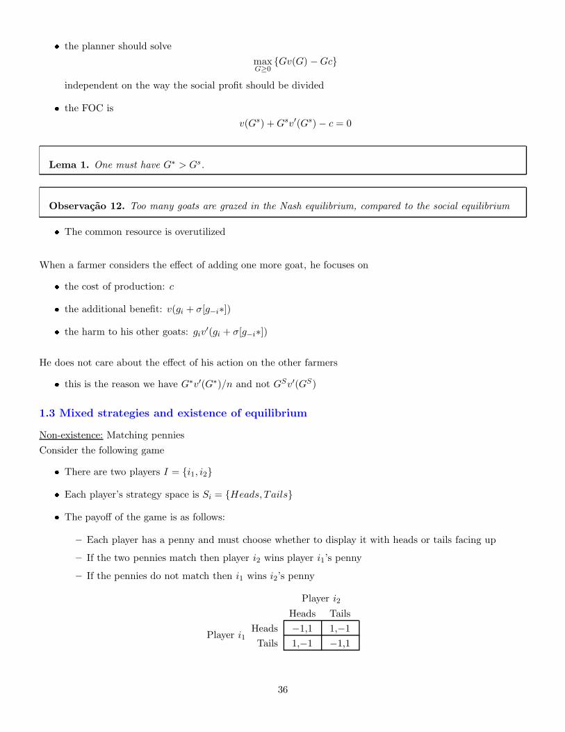
� There are two players I = {i1, i2}
� Each player’s strategy space is Si = {Heads, Tails}
� The payoff of the game is as follows:
– Each player has a penny and must choose whether to display it with heads or tails facing up
– If the two pennies match then player i2 wins player i1’s penny
– If the pennies do not match then i1 wins i2’s penny
Player i1
Player i2
Heads Tails
Heads −1,1 1,−1
Tails 1,−1 −1,1
36
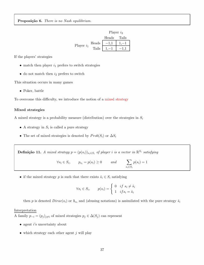
Proposicao 6. There is no Nash equilibrium.
Player i1
Player i2
Heads Tails
Heads −1,1 1,−1
Tails 1,−1 −1,1
If the players’ strategies
� match then player i1 prefers to switch strategies
� do not match then i2 prefers to switch
This situation occurs in many games
� Poker, battle
To overcome this difficulty, we introduce the notion of a mixed strategy
Mixed strategies
A mixed strategy is a probability measure (distribution) over the strategies in Si
� A strategy in Si is called a pure strategy
� The set of mixed strategies is denoted by Prob(Si) or ∆Si
Definicao 11. A mixed strategy p = (p(si))si∈Siof player i is a vector in R
Si satisfying
∀si ∈ Si, psi = p(si) ≥ 0 and∑
si∈Si
p(si) = 1
� if the mixed strategy p is such that there exists si ∈ Si satisfying
∀si ∈ Si, p(si) =
{
0 if si 6= si
1 ifsi = si
then p is denoted Dirac(si) or 1si and (abusing notations) is assimilated with the pure strategy si
Interpretation
A family p−i = (pj)j 6=i of mixed strategies pj ∈ ∆(Sj) can represent
� agent i’s uncertainty about
� which strategy each other agent j will play
37
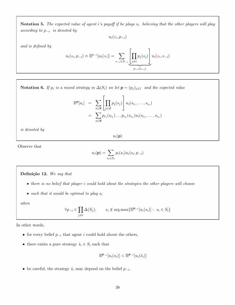
Notation 5. The expected value of agent i’s payoff if he plays si believing that the other players will play
according to p−i is denoted by
ui(si, p−i)
and is defined by
ui(si, p−i) ≡ Ep−i [ui(si)] =
∑
s−i∈S−i
∏
j 6=i
pj(sj)
︸ ︷︷ ︸
p−i(s−i)
ui(si, s−i)
Notation 6. If pi is a mixed strategy in ∆(Si) we let p = (pj)j∈I and the expected value
Ep[ui] =
∑
s∈S
∏
j∈J
pj(sj)
ui(si1 , . . . , sin)
=∑
s∈S
pi1(si1) . . . pin(sin)ui(si1 , . . . , sin)
is denoted by
ui(p)
Observe that
ui(p) =∑
si∈Si
pi(si)ui(si, p−i)
Definicao 12. We say that
� there is no belief that player i could hold about the strategies the other players will choose
� such that it would be optimal to play si
when
∀p−i ∈∏
j 6=i
∆(Sj), si /∈ argmax{Ep−i [ui(si)] : si ∈ Si}
In other words,
� for every belief p−i that agent i could hold about the others,
� there exists a pure strategy si ∈ Si such that
Ep−i [ui(si)] < E
p−i [ui(si)]
� be careful, the strategy si may depend on the belief p−i.
38
Proposicao 7. Assume that the pure strategy si is strictly dominated by the pure strategy σi
∀s−i ∈ S−i, ui(si, s−i) < ui(σi, s−i)
Then
� there is no belief that player i could hold about the strategies the other players will choose such that
it would be optimal to play si.
More precisely, for every family p−i = (pj)j 6=i of mixed strategies pj ∈ ∆(Sj), we have
Ep−i [ui(si)] < E
p−i [ui(σi)]
In this case, the strategy σi improves the expected payoff independently of the belief p−i agent i holds about
the other players’ actions
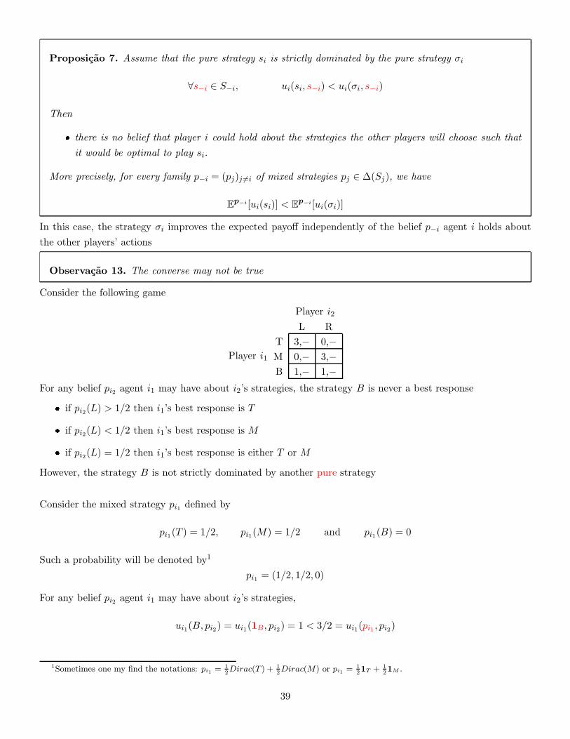
Observacao 13. The converse may not be true
Consider the following game
Player i1
Player i2
L R
T 3,− 0,−M 0,− 3,−B 1,− 1,−
For any belief pi2 agent i1 may have about i2’s strategies, the strategy B is never a best response
� if pi2(L) > 1/2 then i1’s best response is T
� if pi2(L) < 1/2 then i1’s best response is M
� if pi2(L) = 1/2 then i1’s best response is either T or M
However, the strategy B is not strictly dominated by another pure strategy
Consider the mixed strategy pi1 defined by
pi1(T ) = 1/2, pi1(M) = 1/2 and pi1(B) = 0
Such a probability will be denoted by1
pi1 = (1/2, 1/2, 0)
For any belief pi2 agent i1 may have about i2’s strategies,
ui1(B, pi2) = ui1(1B , pi2) = 1 < 3/2 = ui1(pi1 , pi2)
1Sometimes one my find the notations: pi1 = 1
2Dirac(T ) + 1
2Dirac(M) or pi1 = 1
21T + 1
21M .
39
Observacao 14. The strategy B is strictly dominated by the mixed strategy pi1 = (1/2, 1/2, 0)
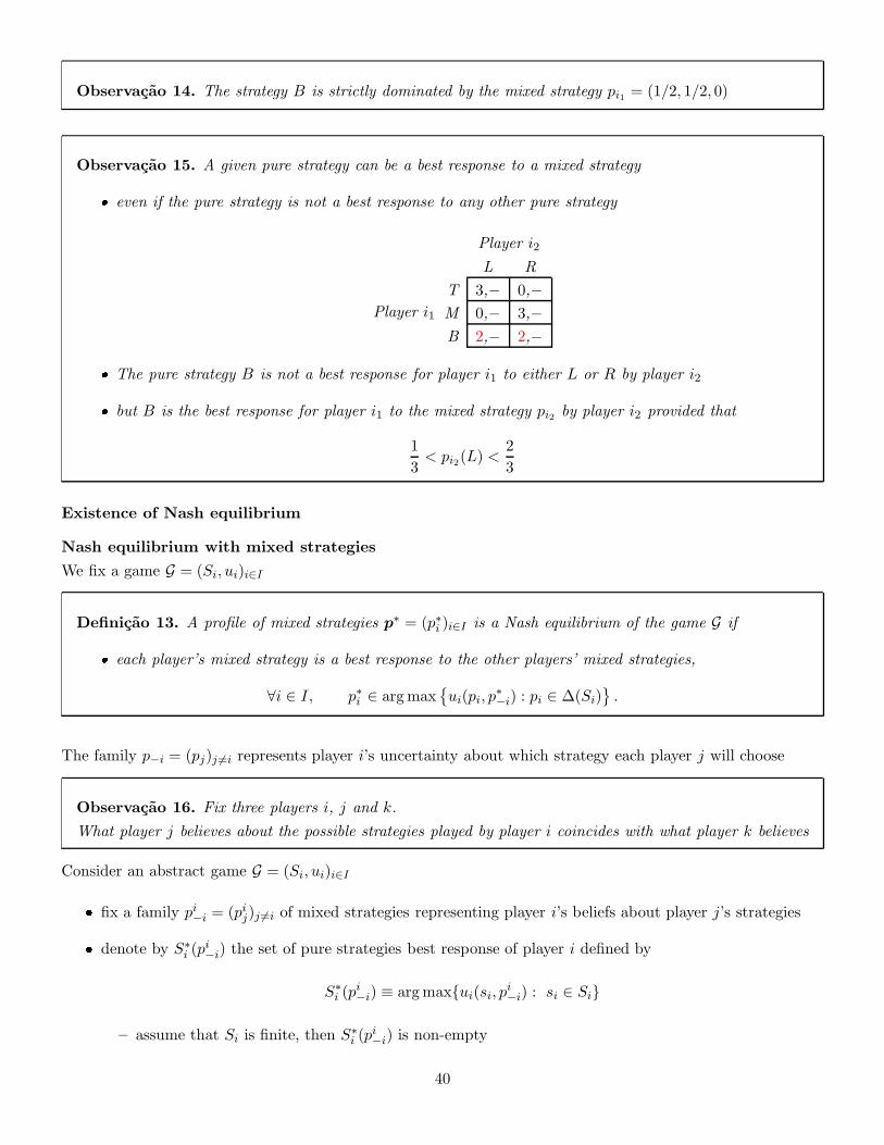
Observacao 15. A given pure strategy can be a best response to a mixed strategy
� even if the pure strategy is not a best response to any other pure strategy
Player i1
Player i2
L R
T 3,− 0,−M 0,− 3,−B 2,− 2,−
� The pure strategy B is not a best response for player i1 to either L or R by player i2
� but B is the best response for player i1 to the mixed strategy pi2 by player i2 provided that
1
3< pi2(L) <
2
3
Existence of Nash equilibrium
Nash equilibrium with mixed strategies
We fix a game G = (Si, ui)i∈I
Definicao 13. A profile of mixed strategies p∗ = (p∗i )i∈I is a Nash equilibrium of the game G if
� each player’s mixed strategy is a best response to the other players’ mixed strategies,
∀i ∈ I, p∗i ∈ argmax{ui(pi, p
∗−i) : pi ∈ ∆(Si)
}.
The family p−i = (pj)j 6=i represents player i’s uncertainty about which strategy each player j will choose
Observacao 16. Fix three players i, j and k.
What player j believes about the possible strategies played by player i coincides with what player k believes
Consider an abstract game G = (Si, ui)i∈I
� fix a family pi−i = (pij)j 6=i of mixed strategies representing player i’s beliefs about player j’s strategies
� denote by S∗i (p
i−i) the set of pure strategies best response of player i defined by
S∗i (p
i−i) ≡ argmax{ui(si, pi−i) : si ∈ Si}
– assume that Si is finite, then S∗i (p
i−i) is non-empty
40
� if pi is a mixed strategy in ∆(Si), we denote by supp pi its support defined by
supp pi = {pi > 0} = {si ∈ Si : pi(si) > 0}
Proposicao 8. A mixed strategy p∗i is a best response to pi−i, i.e.,
p∗i ∈ argmax{ui(pi, pi−i) : pi ∈ ∆(Si)}
if and only if the support of p∗i is a subset of all pure strategies that are best response to pi−i, i.e.,
{si ∈ Si : p∗i (si) > 0} ≡ supp p∗i ⊂ S∗
i (pi−i)
In other words the set
argmax{ui(pi, pi−i) : pi ∈ ∆(Si)}
of best responses to pi−i coincides with
Prob(S∗i (p
i−i)) = ∆(S∗
i (pi−i))
NE with mixed strategies: An equivalent definition
Teorema 7. A profile of mixed strategies p∗ = (p∗i )i∈I is a Nash equilibrium of the game G if and only if
� for every player i every pure strategy in the support of p∗i is a best response to the other players’ mixed
strategies
∀i ∈ I, supp p∗i ⊂ argmax{ui(si, p∗−i) : si ∈ Si}
Interpretation 8. Players
� have identical beliefs about other players’ possible actions or strategies
� choose best response strategies consistent with these beliefs
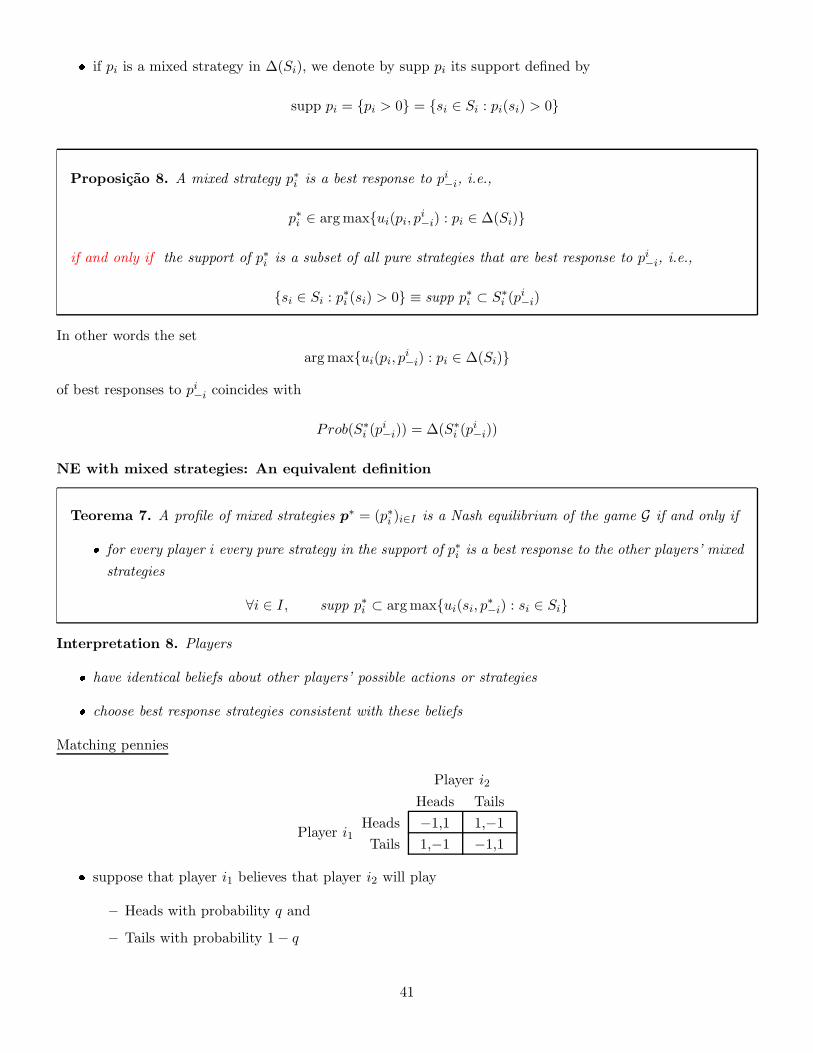
Matching pennies
Player i1
Player i2
Heads Tails
Heads −1,1 1,−1
Tails 1,−1 −1,1
� suppose that player i1 believes that player i2 will play
– Heads with probability q and
– Tails with probability 1− q
41
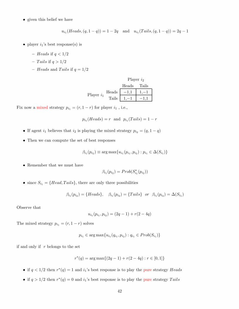
� given this belief we have
ui1(Heads, (q, 1 − q)) = 1− 2q and ui1(Tails, (q, 1 − q)) = 2q − 1
� player i1’s best response(s) is
– Heads if q < 1/2
– Tails if q > 1/2
– Heads and Tails if q = 1/2
Player i1
Player i2
Heads Tails
Heads −1,1 1,−1
Tails 1,−1 −1,1
Fix now a mixed strategy pi1 = (r, 1 − r) for player i1 , i.e.,
pi1(Heads) = r and pi1(Tails) = 1− r
� If agent i1 believes that i2 is playing the mixed strategy pi2 = (q, 1− q)
� Then we can compute the set of best responses
βi1(pi2) ≡ argmax{ui1(pi1 , pi2) : pi1 ∈ ∆(Si1)}
� Remember that we must have
βi1(pi2) = Prob(S∗i1(pi2))
� since Si1 = {Head, Tails}, there are only three possibilities
βi1(pi2) = {Heads}, βi1(pi2) = {Tails} or βi1(pi2) = ∆(Si1)
Observe that
ui1(pi1 , pi2) = (2q − 1) + r(2− 4q)
The mixed strategy pi1 = (r, 1 − r) solves
pi1 ∈ argmax{ui1(qi1 , pi2) : qi1 ∈ Prob(Si1)}
if and only if r belongs to the set
r∗(q) = argmax{(2q − 1) + r(2− 4q) : r ∈ [0, 1]}
� if q < 1/2 then r∗(q) = 1 and i1’s best response is to play the pure strategy Heads
� if q > 1/2 then r∗(q) = 0 and i1’s best response is to play the pure strategy Tails
42
� if q = 1/2 then r∗(q) = [0, 1] and any mixed strategy is a best response, i.e., i1 is indifferent between
Heads and Tails
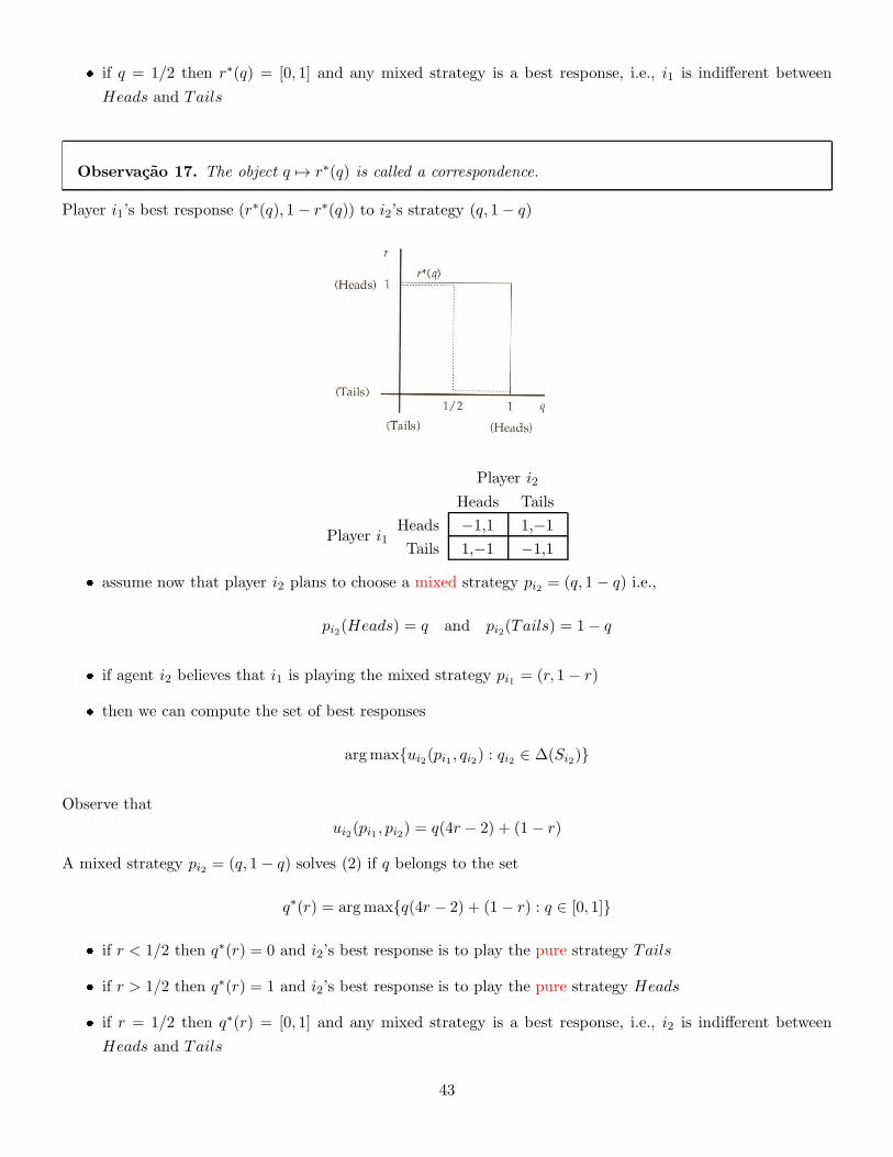
Observacao 17. The object q 7→ r∗(q) is called a correspondence.
Player i1’s best response (r∗(q), 1 − r∗(q)) to i2’s strategy (q, 1− q)
Player i1
Player i2
Heads Tails
Heads −1,1 1,−1
Tails 1,−1 −1,1
� assume now that player i2 plans to choose a mixed strategy pi2 = (q, 1 − q) i.e.,
pi2(Heads) = q and pi2(Tails) = 1− q
� if agent i2 believes that i1 is playing the mixed strategy pi1 = (r, 1 − r)
� then we can compute the set of best responses
argmax{ui2(pi1 , qi2) : qi2 ∈ ∆(Si2)}
Observe that
ui2(pi1 , pi2) = q(4r − 2) + (1− r)
A mixed strategy pi2 = (q, 1− q) solves (2) if q belongs to the set
q∗(r) = argmax{q(4r − 2) + (1− r) : q ∈ [0, 1]}
� if r < 1/2 then q∗(r) = 0 and i2’s best response is to play the pure strategy Tails
� if r > 1/2 then q∗(r) = 1 and i2’s best response is to play the pure strategy Heads
� if r = 1/2 then q∗(r) = [0, 1] and any mixed strategy is a best response, i.e., i2 is indifferent between
Heads and Tails
43
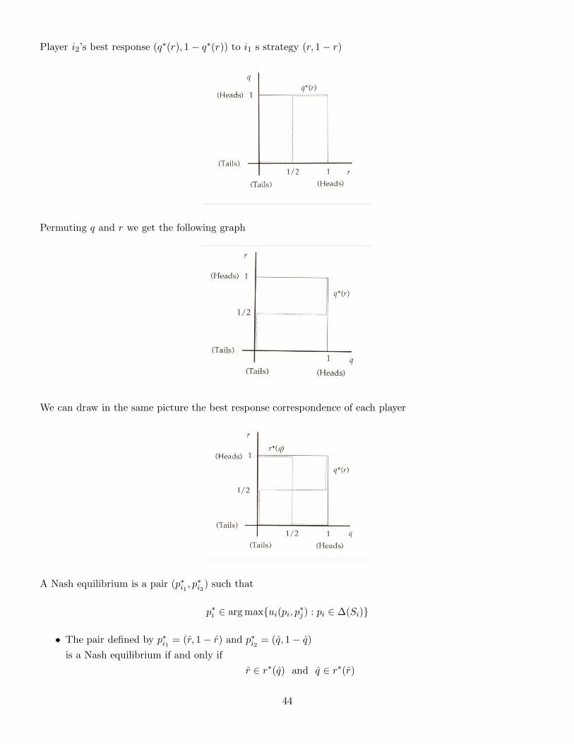
Player i2’s best response (q∗(r), 1 − q∗(r)) to i1 s strategy (r, 1 − r)
Permuting q and r we get the following graph
We can draw in the same picture the best response correspondence of each player
A Nash equilibrium is a pair (p∗i1 , p∗i2) such that
p∗i ∈ argmax{ui(pi, p∗j) : pi ∈ ∆(Si)}
� The pair defined by p∗i1 = (r, 1 − r) and p∗i2 = (q, 1− q)
is a Nash equilibrium if and only if
r ∈ r∗(q) and q ∈ r∗(r)
44

� The unique Nash equilibrium of the Matching Pennies is then
pi1 = (1/2, 1/2) and pi2 = (1/2, 1/2)
The battle of sexes
Chris
Pat
Opera Fight
Opera 2,1 0,0
Fight 0,0 1,2
Denote by
� (q, 1− q) the mixed strategy in which Pat plays Opera with probability q
� (r, 1 − r) the mixed strategy in which Chris plays Opera with probability r
3 NE with mixed strategies
1. Pat and Chris play the pure strategy Opera
2. Pat and Chris play the pure strategy Fight
3. Pat plays the mixed strategy where Opera is chosen with probability 1/3 and Chris plays the mixed
strategy where Opera is chosen with probability 2/3
2 players with 2 pure strategies
Consider the problem of defining player i1’s best response (r, 1 − r) when player i2 plays (q, 1− q)
Player i1
Player i2
Left Right
Up x,− y,−Down z,− w,−
We discuss the four following cases
(i) x > z and y > w
45
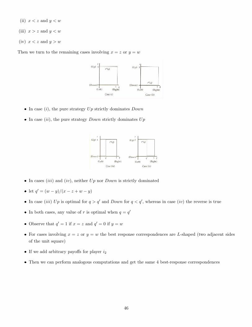
(ii) x < z and y < w
(iii) x > z and y < w
(iv) x < z and y > w
Then we turn to the remaining cases involving x = z or y = w
� In case (i), the pure strategy Up strictly dominates Down
� In case (ii), the pure strategy Down strictly dominates Up
� In cases (iii) and (iv), neither Up nor Down is strictly dominated
� let q′ = (w − y)/(x− z + w − y)
� In case (iii) Up is optimal for q > q′ and Down for q < q′, whereas in case (iv) the reverse is true
� In both cases, any value of r is optimal when q = q′
� Observe that q′ = 1 if x = z and q′ = 0 if y = w
� For cases involving x = z or y = w the best response correspondences are L-shaped (two adjacent sides
of the unit square)
� If we add arbitrary payoffs for player i2
� Then we can perform analogous computations and get the same 4 best-response correspondences
46

� Fix any of the four best response correspondence for player i1
� Fix any of the four best response correspondence for player i2
� Checking all 16 possible pairs, there is always at least one intersection
We obtain the following qualitative features that can result: There can be
� a single pure strategy Nash equilibrium
� a single mixed strategy equilibrium
� 2 pure strategy equilibria and a single mixed strategy equilibrium
Nash existence result
Teorema 9 (Nash). Consider a game G = (Si, ui)i∈I . If for each player i the set of pure strategies Si is
finite then there exists at least one Nash equilibrium with mixed strategies.
47
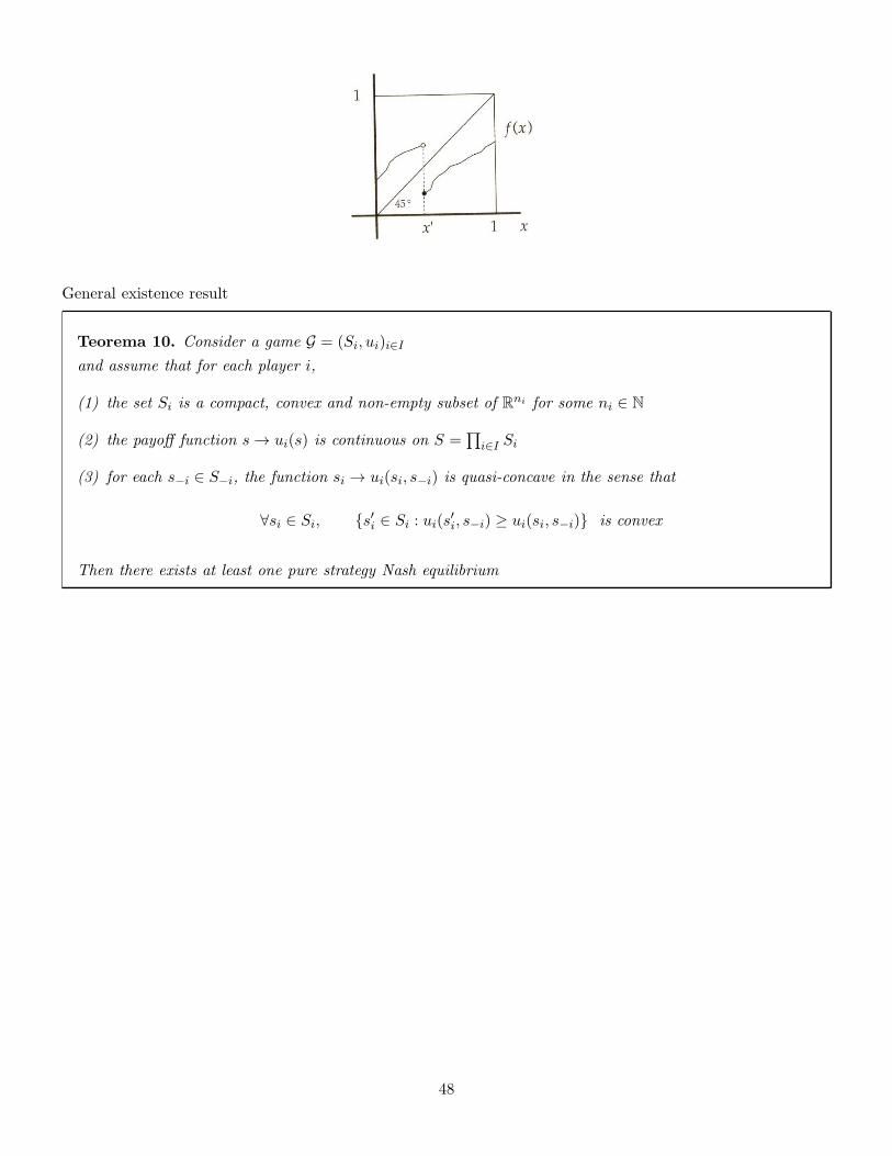
General existence result
Teorema 10. Consider a game G = (Si, ui)i∈I
and assume that for each player i,
(1) the set Si is a compact, convex and non-empty subset of Rni for some ni ∈ N
(2) the payoff function s → ui(s) is continuous on S =∏
i∈I Si
(3) for each s−i ∈ S−i, the function si → ui(si, s−i) is quasi-concave in the sense that
∀si ∈ Si, {s′i ∈ Si : ui(s′i, s−i) ≥ ui(si, s−i)} is convex
Then there exists at least one pure strategy Nash equilibrium
48
Cap. 2 - Dynamic games of complete information
2.1 Dynamic games of complete and perfect information
Theory: Backwards induction
Important words
� we introduce dynamic games
� restrict our attention to games with complete information
– the players’ payoff functions are common knowledge
� in this chapter we analyze dynamic games with complete but also perfect information
– at each move in the game
– the player with the move knows the full history of the play of the game thus far
� the central issue in dynamic games is credibility
An example:
Consider the following 2-move game
1. player i1 chooses between giving player i2 $1,000 and giving player i2 nothing
2. player i2 observes player i1’s move and then chooses whether or not to explode a grenade that will kill
both players
Suppose that player i2 threatens to explode the grenade unless player i1 pays the $1, 000
� if player i1 believes the threat, then
player i1’s best response is to pay the $1, 000
� but player i1 should not believe the threat, because it is not credible:
– if player i2 were given the opportunity to carry out the threat
– player i2 would choose not to carry it out
� player i1 should pay player i2 nothing
The framework
We analyze in this chapter the following class of dynamic games with complete and perfect information
� there are 2 players and 2 moves
� first, player i1 moves
49
� then player i2 observes player i1’s move
� then player i2 moves and the game ends
Description of a specific class of games
1. player i1 chooses an action ai1 from a feasible set Ai1
2. player i2 observes ai1 and then chooses an action ai2 from a feasible set Ai2
3. payoffs are ui1(ai1 , ai2) and ui2(ai1 , ai2)
Other dynamic games with complete and perfect information
The key features of a dynamic game of complete and perfect information are that
1. the moves occur in sequence
2. all previous moves are observed before the next move is chosen
3. the players’ payoffs from each feasible combination of moves are common knowledge
Backwards induction
We solve a game from this class by backwards induction as follows:
� when player i2 gets the move at the second stage of the game
� he will face the following problem
maxai2∈Ai2
{ui2(ai1 , ai2) : ai1 given}
� assume that for each ai1 ∈ Ai1 , player i2’s optimization problem has a unique solution, denoted by Ri2(ai1)
– this is player i2’s reaction (or best response) to player i1’s action
� recall that payoffs are common knowledge
– therefore player i1 can solve i2’s problem as well as i2 can
� player i1 will anticipate player i2’s reaction to each action ai1 that i1 might take
� thus player i1’s problem at the first stage amounts to
maxai1∈Ai1
{ui1(ai1 , Ri2(ai1))}
� assume that the previous optimization problem for i1 also has a unique solution, denoted by a∗i1
50

Definicao 14. The pair of actions (a∗i1 , Ri2(a∗i1)) is called the backwards induction outcome of this game
Backwards induction and credible threats
� the backwards induction outcome does not involve non-credible threats
� player i1 anticipates that player i2 will respond optimally to any action ai1 that i1 might choose, by
playing Ri2(ai1)
� player i1 gives no credence to threats by player i2 to respond in ways that will not be in i2’s self-interest
when the second stage arrives
A 3-move game
Consider the following 3-move game: player i1 moves twice
1. Player i1 chooses L or R
� L ends the game with payoffs of 2 to i1 and 0 to i2
2. Player i2 observes i1’s choice:
if i1 chose R then i2 can choose between L′ and R′
� L′ ends the game with payoffs of 1 to both players
3. Player i1 observes i2’s choice2:
if the earlier choices were R and R′ then i1 chooses L′′ of R′′, both of which end the game
� L′′ with payoffs of 3 to player i1 and 0 to player i2
� R′′ with payoffs of 0 to player i1 and 2 to player i2
2And recalls his own choice in the first stage
51
Let’s compute the backwards induction outcome of this game
� we begin at the third stage, i.e., player i1’s second move
– the strategy L′′ is optimal
� at the second stage, player i2 anticipates that if the game reaches the third stage then i1 will play L′′
– payoff of 1 from action L′
– payoff of 0 from action R′
at the second stage, the optimal action for player i2 is L′
� at the first stage, player i1 anticipates that if the game reaches the second stage then i2 will play L′
– payoff of 2 from action L
– payoff of 1 from action R
the first stage choice for player i1 is L, thereby ending the game
Stackelberg model of duopoly
Von Stackelberg (1934) proposed a dynamic model of duopoly
� a dominant (leader) firm moves first
� a subordinate (follower) firm moves second
At some points in the history of the U.S. automobile history, for example, General Motors has seemed to play
such a leadership role
� as in the Cournot model, Stackelberg assumes that firms choose quantities
Timing of the game
1. firm i1 chooses the quantity qi1
2. firm i2 observes qi1 and then chooses a quantity qi2
3. the payoff to firm i is given by the profit function
πi(qi, qj) = qi[P (Q)− c]
where
52
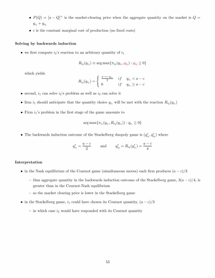
� P (Q) = [a − Q]+ is the market-clearing price when the aggregate quantity on the market is Q =
qi1 + qi2
� c is the constant marginal cost of production (no fixed costs)
Solving by backwards induction
� we first compute i2’s reaction to an arbitrary quantity of i1
Ri2(qi1) ≡ argmax{πi2(qi1 , qi2) : qi2 ≥ 0}
which yields
Ri2(qi1) =
{a−c−qi1
2 if qi1 < a− c
0 if qi1 ≥ a− c
� second, i1 can solve i2’s problem as well as i2 can solve it
� firm i1 should anticipate that the quantity choice qi1 will be met with the reaction Ri2(qi1)
� Firm i1’s problem in the first stage of the game amounts to
argmax{πi1(qi1 , Ri2(qi1)) : qi1 ≥ 0}
� The backwards induction outcome of the Stackelberg duopoly game is (q∗i1 , q∗i2) where
q∗i1 =a− c
2and q∗i2 = Ri2(q
∗i1) =
a− c
4
Interpretation
� in the Nash equilibrium of the Cournot game (simultaneous moves) each firm produces (a− c)/3
– thus aggregate quantity in the backwards induction outcome of the Stackelberg game, 3(a− c)/4, is
greater than in the Cournot-Nash equilibrium
– so the market clearing price is lower in the Stackelberg game
� in the Stackelberg game, i1 could have chosen its Cournot quantity, (a− c)/3
– in which case i2 would have responded with its Cournot quantity
53
� in the Stackelberg game, i1 could have achieved its Cournot profit level but chose to do otherwise
� so i1’s profit in the Stackelberg game must exceed its profit in the Cournot game
� but because the market clearing price is lower in the Stackelberg game
� the aggregate profits are lower wrt. the Cournot outcome
� therefore, the fact that i1 is better off implies that i2 is worse off
Observacao 18. In game theory, having more information can make a player worse off.
� more precisely, having it known to the other players that one has more information can make a player
worse off
� in the Stackelberg game, the information in question is i1’s quantity
� firm i2 knows i1’s action qi1
� and firm i1 knows that i2 knows qi1
Wages and employment in a unionized firm
Leontief (1946) proposed the following model of the relationship between a firm and a monopoly union
� The union is the monopoly seller of labor to the firm
� The union has exclusive control over wages
� But the firm has exclusive control over employment
� The union’s utility function is U(w,L) where
– w is the wage the union demands from the firm
– L is employment
� We assume that (w,L) → U(w,L) is increasing in both w and L
� The firm’s profit function is
π(w,L) ≡ R(L)− wL
– R(L): revenue the firm can earn if it employs L workers
� We assume that L 7→ R(L) is
– twice continuously differentiable
54
– strictly increasing (i.e., R′ > 0)
– strictly concave (i.e., R′′ < 0) and
– satisfies Inada’s condition at 0 and ∞, i.e.,
limL→0+
R′(L) = ∞ and limL→∞
R(L) = 0
Timing of the game
1. The union makes a wage demand, w
2. The firm observes and accepts w and then chooses employment, L
3. Payoffs are U(w,L) and π(w,L)
Backwards induction outcome of the game
� First, we can characterize the firm’s best response L∗(w) in stage 2 to an arbitrary wage demand w by
the union in stage 1
� Given w the firm chooses L∗(w) to solve
L∗(w) ≡ argmax{π(w,L) : L ≥ 0}
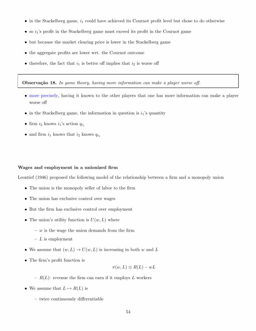
� If w > 0 then there is a unique solution L∗(w) satisfying
R′(L∗(w)) = w
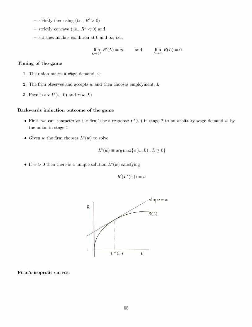
Firm’s isoprofit curves:
55
Fixing the wage level w′ on the vertical line
� the firm’s choice of L is a point on the horizontal line {(L,w′) : L ≥ 0}
� Holding L fixed, the firm does better when w is lower
– optimal L is such that the isoprofit curve through (L,w) is tangent to the constraint {(L,w′) : L ≥ 0}
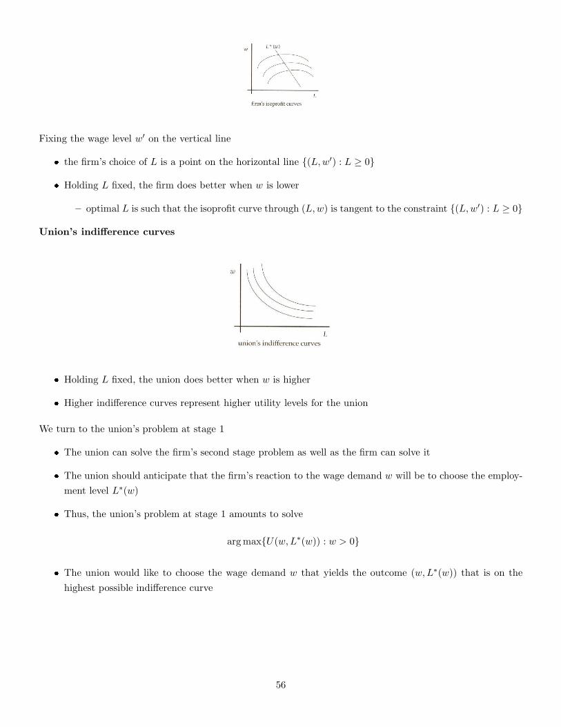
Union’s indifference curves
� Holding L fixed, the union does better when w is higher
� Higher indifference curves represent higher utility levels for the union
We turn to the union’s problem at stage 1
� The union can solve the firm’s second stage problem as well as the firm can solve it
� The union should anticipate that the firm’s reaction to the wage demand w will be to choose the employ-
ment level L∗(w)
� Thus, the union’s problem at stage 1 amounts to solve
argmax{U(w,L∗(w)) : w > 0}
� The union would like to choose the wage demand w that yields the outcome (w,L∗(w)) that is on the
highest possible indifference curve
56
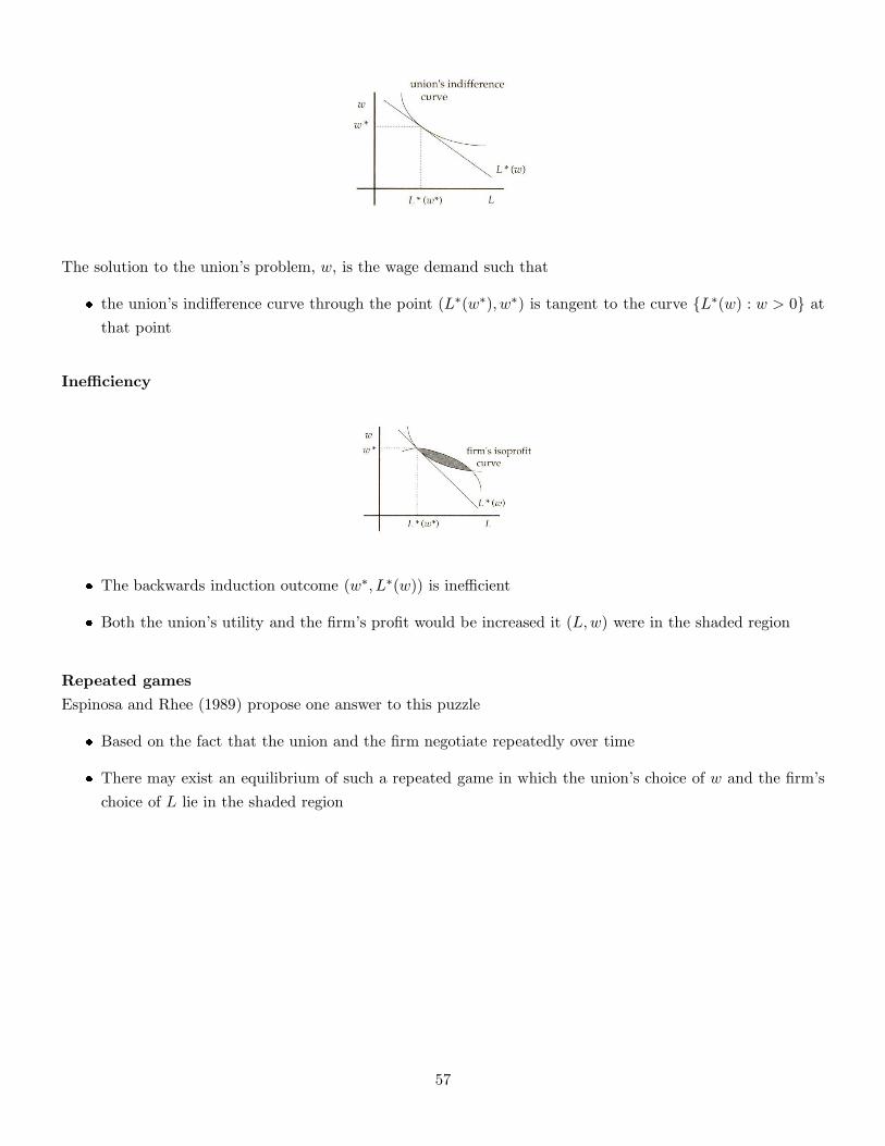
The solution to the union’s problem, w, is the wage demand such that
� the union’s indifference curve through the point (L∗(w∗), w∗) is tangent to the curve {L∗(w) : w > 0} at
that point
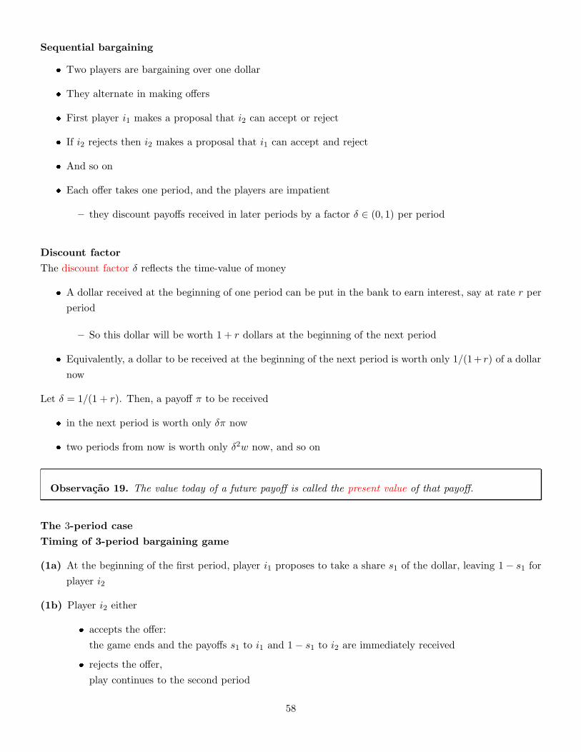
Inefficiency
� The backwards induction outcome (w∗, L∗(w)) is inefficient
� Both the union’s utility and the firm’s profit would be increased it (L,w) were in the shaded region
Repeated games
Espinosa and Rhee (1989) propose one answer to this puzzle
� Based on the fact that the union and the firm negotiate repeatedly over time
� There may exist an equilibrium of such a repeated game in which the union’s choice of w and the firm’s
choice of L lie in the shaded region
57
Sequential bargaining
� Two players are bargaining over one dollar
� They alternate in making offers
� First player i1 makes a proposal that i2 can accept or reject
� If i2 rejects then i2 makes a proposal that i1 can accept and reject
� And so on
� Each offer takes one period, and the players are impatient
– they discount payoffs received in later periods by a factor δ ∈ (0, 1) per period
Discount factor
The discount factor δ reflects the time-value of money
� A dollar received at the beginning of one period can be put in the bank to earn interest, say at rate r per
period
– So this dollar will be worth 1 + r dollars at the beginning of the next period
� Equivalently, a dollar to be received at the beginning of the next period is worth only 1/(1+ r) of a dollar
now
Let δ = 1/(1 + r). Then, a payoff π to be received
� in the next period is worth only δπ now
� two periods from now is worth only δ2w now, and so on
Observacao 19. The value today of a future payoff is called the present value of that payoff.
The 3-period case
Timing of 3-period bargaining game
(1a) At the beginning of the first period, player i1 proposes to take a share s1 of the dollar, leaving 1− s1 for
player i2
(1b) Player i2 either
� accepts the offer:
the game ends and the payoffs s1 to i1 and 1− s1 to i2 are immediately received
� rejects the offer,
play continues to the second period
58
(2a) At the beginning of the second period, i2 proposes that player i1 take a share s2 of the dollar,3 leaving
1− s2 for i2
(2b) Player i1 either
� accepts the offer:
the game ends and the payoffs s2 to i1 and 1− s2 to i2 are immediately received
� rejects the offer:
play continues to the third period
(3) At the beginning of the third period,
� i1 receives a share s of the dollar
� i2 receives a share 1− s of the dollar
where s ∈ (0, 1) is exogenously given
Backwards induction outcome
We first compute i2’s optimal offer if the second period is reached
� Player i1 can receive s in the third period by rejecting i2’s offer of s2 this period
� But the value this period of receiving s next period is only δs
� Thus, i1 will
– accept s2 if s2 ≥ δs
– reject s2 if s2 < δs
� We assume that each player will accept an offer if indifferent between accepting and rejecting
� Player i2’s decision problem in the second period amounts to choosing between
– receiving 1− δs this period by offering s2 = δs to player i1
– receiving 1− s next period by offering player i1 any s2 < δs
� The discounted value of the latter decision is δ(1 − s),
– which is less than 1− δs available from the former option
� So player i2’s optimal second-period offer is s∗2 = δs
3st always goes to player i1 regardless of who made the offer
59
Observacao 20. If play reaches the second period, player i2 will offer s∗2 and player i1 will accept.
� Since i1 can solve i2’s second-period problem as well as player i2 can
� Then i1 knows that i2 can receive 1− s∗2 in the second period by rejecting i1’s offer of s1 this period
� The value this period of receiving 1− s∗2 next period is only δ(1 − s∗2)
� Thus player i2 will accept i1’s offer of s1 this period ⇔
1− s1 ≥ δ(1− s∗2) or s1 ≤ 1− δ(1 − s∗2)
� Player i1’s first-period decision problem therefore amounts to choosing between
– receiving 1− δ(1 − s∗2) this period by offering 1− s1 = δ(1 − s∗2) to i2
– receiving s∗2 next period by offering 1− s1 < δ(1 − s∗2) to i2
� The discounted value of the latter option is δs∗2 = δ2s
– which is less than the 1− δ(1 − s∗2) = 1− δ(1 − δs) available from the former option
� Thus player i1’s optimal first-period offer is
s∗1 = 1− δ(1 − s∗2) = 1− δ(1 − δs)
Observacao 21. The backwards induction outcome of this 3-period game is
� i1 offers the settlement (s∗1, 1− s∗1) to i2, who accepts
The infinite horizon case
� The timing is as described previously
� Except that the exogenous settlement in step (3) is replaced by an infinite sequence of steps (3a), (3b),
(4a), (4b), and so on
– Player i1 makes the offer in odd-numbered period
– Player i2 in even-numbered
� Bargaining continues until one player accepts an offer
� We would like to solve backwards
� Because the game could go on infinitely, there is no last move at which to begin such an analysis
60
A solution was proposed by Shaked and Sutton (1984)
� The game beginning in the third period (should it be reached) is identical to the game as a whole (beginning
in the first period)
� In both cases (game beginning in the 3° period or as a whole)
– player i1 makes the first offer
– the players alternate in making subsequent offers
– the bargaining continues until one player accepts an offer
� Suppose that there is a backwards induction outcome of the game as a whole in which players i1 and i2
receive the payoffs s and 1− s
� We can use these payoffs in the game beginning in the third period, should it be reached
� And then work backwards to the first period, as in the 3-period model, to compute a new backwards
induction outcome for the game as a whole
� In this new backwards induction outcome, i1 will offer the settlement (f(s), 1 − f(s)) in the first period
and i2 will accept, where
f(s) = 1− δ(1− δs)
� Let sH be the highest payoff player i1 can achieve in any backwards induction outcome of the game as a
whole
� Using sH as the third-period payoff to player i1, this will produce a new backwards induction outcome in
which player i1’s first-period payoff is f(sH)
� Since s 7→ f(s) = 1− δ + δ2s is increasing, the payoff f(sH) must coincide with sH
� The only value of s that satisfies f(s) = s is 1/(1 + δ), which will be denoted by s∗
� Actually we can prove that (s∗, 1− s∗) is the unique backwards-induction outcome of the game as a whole
– In the first period, i1 offers the settlement (s∗, 1− s∗)
– Player i2 accepts
2.2 Two-stage games of complete but imperfect information
Theory: Subgame perfection
� We continue to assume that play proceeds in a sequence of stages
� The moves in all previous stages are observed before the next stage begins
� However, we now allow there be simultaneous moves within each stage
61

– The game has imperfect information
We will analyze the following simple game:
1. Players i1 and i2 simultaneously choose actions ai1 and ai2 from feasible sets Ai1 and Ai2 , respectively
2. Players i3 and i4 observe the outcome of the first stage, (ai1 , ai2), and then simultaneously choose actions
ai3 and ai4 from feasible sets Ai3 and Ai4 , respectively
3. Payoffs are ui(ai1 , ..., ai4)
� The feasible action sets of players i3 and i4 in the second stage, Ai3 and Ai4 , could be allowed to depend
on the outcome of the first stage, (ai1 , ai2)
� In particular, there may be values of (ai1 , ai2) that end the game
� One could allow for a longer sequence of stages either by allowing players to move in more than one stage
or by adding players
� In some applications, players i3 and i4 are players i1 and i2
� In other applications, either player i2 or player i4 is missing
� We solve the game by using an approach in the spirit of backwards induction
� The first step in working backwards from the end of the game involves solving a simultaneous-move game
between players i3 and i4 in stage 2, given the outcome of stage 1
� We will assume that for each feasible outcome (ai1 , ai2) of the first game, the second-stage game that
remains between players i3 and i4 has a unique Nash equilibrium denoted by (ai3(ai1 , ai2), ai4(ai1 , ai2))
62
� If i1 and i2 anticipate that the second-stage behavior of i3 and i4 will be given by the functions ai3 and
ai4
� Then the first-stage interaction between i1 and i2 amounts to the following simultaneous-move game
1. Players i1 and i2 simultaneously choose actions ai1 and ai2 from feasible sets Ai1 and Ai2 , respectively
2. Payoffs are
ui(ai1 , ai2 , ai3(ai1 , ai2), ai4(ai1 , ai2))
� Suppose (a∗i1 , a∗i2) is the unique Nash equilibrium of this simultaneous-move game
� We will call
(a∗i1 , a∗i2, a∗i3 , a
∗i4)
the subgame-perfect outcome of this two-stage game, where
a∗i3 = ai3(a∗i1, a∗i2) and a∗i4 = ai4(a
∗i1, a∗i2)
Attractive feature 11.
� Players i1 and i2 should not believe a threat by players i3 and i4 that the latter will respond with actions
that are not a Nash equilibrium in the remaining second-stage game
� Because when play actually reaches the second stage at least one of i3 and i4 will not want to carry out
such a threat exactly because it is not a best response
Unattractive feature 12.
� Suppose player i1 is also player i3 and that player i1 does not play a∗i1 in the first stage
� Player i4 may then want to reconsider the assumption that player i3 (i.e., player i1 ) will play ai3(ai1 , ai2)
in the second stage
Bank runs
Diamond and Dybvig (1983)
� Two investors have each deposited D with a bank
� The bank has invested the deposits 2D in a long-term project
� If the bank is forced to liquidate its investment before the project matures, a total of α(2D) can be
recovered, where1
2< α < 1
63

� If the bank allows the investment to reach maturity, the project will pay out a total of β(2D), where
β > 1
� There are two dates at which investors can make withdrawals from the bank
– date 1 is before the bank’s investment matures
– date 2 is after
� For simplicity we assume that there is no discounting
� If both investors make withdrawals at date 1 then each receives αD and the game ends
� If only one investor makes a withdrawal at date 1
– then that investor receives the whole deposit D,
– the other receives (2α− 1)D,
– and the game ends
� Finally, if neither investor makes a withdrawal at date 1 then the project matures and the investors make
withdrawal decisions at date 2
� If both investors make withdrawals at date 2 then each receives βD > D and the game ends
� If only one investor makes a withdrawal at date 2 then that investor receives (2β − 1)D > βD, the other
receives D, and the game ends
� Finally if neither investor makes a withdrawal at date 2 then the bank returns βD to each investor and
the game ends
withdraw don’t withdraw
withdraw αD,αD D, (2α − 1)D
don’t withdraw (2α − 1)D,D next stage
withdraw don’t withdraw
withdraw βD, βD (2β − 1)D,D
don’t withdraw D, (2β − 1)D βD, βD
� To analyze this game, we work backwards
� Consider the normal-form game at date 2
� The strategy withdraw strictly dominates don’t withdraw
� There is a unique Nash equilibrium in this game: both investors withdraw, leading to a payoff of (βD, βD)
� Since there is no discounting, we can simply substitute this payoff into the normal-form game at date 1
64

Date 1
withdraw don’t withdraw
withdraw αD,αD D, (2α − 1)D
don’t withdraw (2α − 1)D,D βD, βD
This one period version of the two-period game has two pure strategy Nash equilibria:
1. both investors withdraw, leading to a payoff of (αD,αD)
2. both investors do not withdraw, leading to a payoff of (βD, βD)
� The original 2-period bank runs game has two subgame perfect outcomes
1. both investors withdraw at date 1, yielding payoffs of (αD,αD)
2. both investors do not withdraw at date 1 but do withdraw at date 2, yielding payoffs of (βD, βD)
at date 2
� The first of these outcomes can be interpreted as a run on the bank
� If investor i1 believes that investor i2 will withdraw at t = 1
– then investor i1’s best response is to withdraw,
– even though both investors would be better off if they waited until date 2 to withdraw
Observacao 22. Since there are two subgame perfect equilibria,
� this model does not predict when bank runs will occur,
� but does show that they can occur as an equilibrium phenomenon
Tariffs and imperfect international competition
� Consider two identical countries, denoted by i1 and i2
� Each country has
– a government that chooses a tariff rate
– a firm that produces output for both home consumption and export
– consumers who buy on the home market from either the home firm or the foreign firm
� If the total quantity on the market in country i is Qi, then the market clearing price is
Pi(Qi) = [a−Qi]+
65
� The firm in country i (called firm i) produces hi for home consumption and ei for export, in particular
we have
Qi = hi + ej
� The firms have a constant marginal cost c and no fixed costs (we assume that c < a)
� The total cost of production for firm i is
Ci(hi, ei) ≡ c(hi + ei)
� The firms also incur tariff costs on exports
– if firm i exports ei to country j
– when government j has set the tariff rate tj
then firm i must pay tjei to government j
Timing
1. The governments simultaneously choose tariff rates, ti1 and ti2
2. The firms observe the tariff rates and simultaneously choose quantities for home consumption and for
export (hi, ei)
3. Payoffs are profit to firms and total welfare to governments
� Profit to firm i is
πi(ti, tj , hi, ei, hj , ej) ≡ [a− (hi + ej)]+hi + [a− (ei + hj)]
+ei
−c(hi + ei)− tjei
� Total welfare to government i,
Wi(ti, tj , hi, ei, hj , ej) ≡1
2Q2
i + πi(ti, tj , hi, ei, hj , ej) + tiej
where total welfare is the sum of
– consumers’ surplus enjoyed by the consumers in country i,
– the profit earned by the firm i, and
– the tariff revenue collected by government i from firm j
Solucao
� Suppose the governments have chosen the tariffs ti1 and ti2
� Assume that (h∗i1 , e∗i1, h∗i2 , e
∗i2) is a Nash equilibrium in the remaining game between firms i1 and i2
66
� Then, for each i, (h∗i , e∗i ) must solve
argmax{πi(ti, tj, hi, ei, h∗j , e∗j ) : hi ≥ 0 and ei ≥ 0}
� Firm i is maximizing profits on market i and market j
– h∗i must solve
argmax{hi[a− (hi + e∗j )]+ − chi : hi ≥ 0}
– e∗i must solve
argmax{ei[a− (ei + h∗j )]+ − (c+ tj)ei : ei ≥ 0}
� Assuming e∗j ≤ a− c, we have
h∗i =1
2(a− e∗j − c)
� Assuming h∗j ≤ a− c− tj, we have
e∗i =1
2(a− h∗j − c− tj)
� We obtain four equations with four unknowns
� If ti ≤ (a− c)/2 for each player i, then the solutions are
h∗i (ti) =a− c+ ti
3and e∗i (tj) =
a− c− 2tj3
67
� In the Cournot game, both firms were choosing the quantity (a− c)/3,
– but this result was derived under the assumption of symmetric marginal costs
� In the equilibrium described above, the governments’ tariff choices make marginal costs asymmetric
– On market i, firm i’s marginal cost is c but firm j’s is c+ ti
– Since firm j’s cost is higher it wants to produce less
– If firm j is going to produce less, then the market-clearing price will be higher, so firm i wants to
produce more
� In equilibrium the function h∗i increases in ti and e∗j decreases (at a faster rate) in ti
� Having solved the second-stage game that remains between the two firms after the governments choose
tariff rates
� We can now represent the first-stage interaction between the two governments as the following simultaneous-
move game
� First, the governments simultaneously choose tariff rates ti1 and ti2
� Second, payoffs are
Wi(ti, tj , h∗i (ti), e
∗i (tj), h
∗j (tj), e
∗j (ti))
� We now solve for the Nash equilibrium of this game between the governments
� We denote by (ti, tj) 7→ W ∗i (ti, tj) the function defined by
W ∗i (ti, tj) ≡ Wi(ti, tj , h
∗i (ti), e
∗i (tj), h
∗j (tj), e
∗j (ti))
� If (t∗i , t∗j ) is a Nash equilibrium of this game between governments then, for each i, the tariff t∗i must solve
argmax{W ∗i (ti, t
∗j ) : ti ≥ 0}
� We propose to show that there exists a solution
(t∗i , t∗j) ∈ (0, (a − c)/2) × (0, (a− c)/2)
� Observe that if ti and t∗j belong to (0, (a − c)/2) then W ∗i (ti, t
∗j) equals
(2(a− c)− ti)2
18+
(a− c+ ti)2
9+
(a− c− 2t∗j )2
9+
ti(a− c− 2ti)
3
� A solution is
t∗i =a− c
3
for each i, independent of t∗j
68
� In this model, choosing a tariff rate of (a− c)/3 is a dominant strategy for each government
� We then obtain the following firms’ quantity choices for the second-stage
h∗i (t∗i ) =
4(a− c)
9and e∗i (t
∗j) =
a− c
9
� Thus, the subgame-perfect outcome of this tariff game is
t∗i1 = t∗i2 =a− c
3, h∗i1 = h∗i2 =
4(a− c)
9and e∗i1 = e∗i2 =
a− c
9
� If the governments had chosen tariff rates equal to 0
� Then the aggregate quantity on each market would have been
Qi =2(a− c)
3
just as in the Cournot model
� The consumers’ surplus on market i is lower when the governments choose their dominant strategy tariffs
than it would be if they chose zero tariffs
� In fact, zero tariffs is socially optimal, i.e., it is the solution of
argmax{W ∗i1(ti1 , ti2) +W ∗
i2(ti1 , ti2) : ti1 ≥ 0 and ti2 ≥ 0}
� There is an incentive for the governments to sign a treaty in which they commit to zero tariffs
Tournaments
Lazear and Rosen (1981)
� Consider two workers J = {j1, j2} and their boss
� Worker j produces output yj = ej + εj
– ej is effort and εj is noise
� Production proceeds as follows:
1. The workers simultaneously choose non-negative effort levels: ej ≥ 0
2. The noise terms εj1 and εj2 are independently drawn from a density f : R → [0,∞) with zero mean
3. The workers’ output are observed but their effort choices are not
� The workers’ wages therefore can depend on their outputs but not directly on their effort levels
� Suppose the boss decides to induce effort by having the workers compete in a tournament
69
� The winner of the tournament is the worker with the higher output
– wH : wage earned by the winner of the tournament
– wL: the wage earned by the loser
� The payoff to a worker from earning wage w and expending effort e is
u(w, e) = w − g(e)
– g(e): disutility under the effort level e
– g : [0,∞) → [0,∞) is twice continuously differentiable and satisfies g′ > 0 (strictly increasing) and
g′′ > 0 (strictly convex)
� The payoff to the boss is yj1 + yj2 − wH − wL
� The boss is player i1 whose action ai1 is choosing the wages to be paid in the tournament, wH and wL
� There is no player i2
� Worker j1 is player i3 and worker j2 is player i4
� Workers observe the wages chosen in the first stage and then simultaneously choose actions ai3 and ai4 ,
namely effort choices ej1 and ej2
� Since outputs (and so also wages) are functions not only of the players actions but also of the noise term
εj1 and εj2 , we work with the players’ expected payoffs according to the density f
� Suppose that the boss has chosen the wages wH and wL
� Let (e∗j1 , e∗j2) be a Nash equilibrium of the remaining game between the workers
� For each j, e∗j must solve
argmax{πj(wH , wL, ej , e∗k) : ej ≥ 0}
where πj(wH , wL, ej , e∗k) is the expected profit defined by
πj(wH , wL, ej , e∗k) = wH Pr{yj(ej) > yk(e
∗k)}+ wL Pr{yj(ej) < yk(e
∗k)} − g(ej)
= (wH − wL) Pr{yj(ej) > yk(e∗k)}+ wL − g(ej)
where yj(ej) = ej + εj and yk(e∗k) = e∗k + εk
� Assume e∗j is strictly positive
� The first-order condition of the maximization problem is
(wH − wL)∂ Pr{yj(ej) > yk(e
∗k)}
∂ej= g′(ej)
70
� The worker j chooses ej such that the marginal disutility of extra effort, g′(ej), equals the marginal gain
from extra effort
Observe that by Bayes’ rule
Prob{yj(ej) > yk(e∗k)} = Prob{εj > e∗k + εk − ej}
=
∫
Prob{εj > e∗k + z − ej |εk = z}f(z)dz
Since εj and εk are independent we have
Prob{εj > e∗k + z − ej |εk = z} = Prob{εj > e∗k + z − ej}
implying that4
Prob{yj(ej) > yk(e∗k)} =
∫
[1− F (e∗k − ej + z)]f(z)dz
The first order condition becomes
(wH − wL)
∫
f(e∗k − ej + z)f(z)dz = g′(ej)
� If we look for symmetric Nash equilibria
e∗j = e∗k = e∗(wH , wL)
we get
(wH − wL)
∫
R
f(z)2dz = g′(e∗(wH , wL))
� Since g is convex, g′ is increasing
– a bigger prize for winning (i.e., a larger value of wH − wL) induces more effort
Observacao 23. Holding the prize constant,
� it is not worthwhile to work hard when output is very noisy,
� because the outcome of the tournament is likely to be determined by luck rather than effort
� If εj is normally distributed with variance σ2, then
∫
f(z)2dz =1
2σ√π
which decreases in σ, so e∗(wH , wL) decreases in σ
� We work backwards to the first stage of the game
4F is the cumulative distribution of f
71
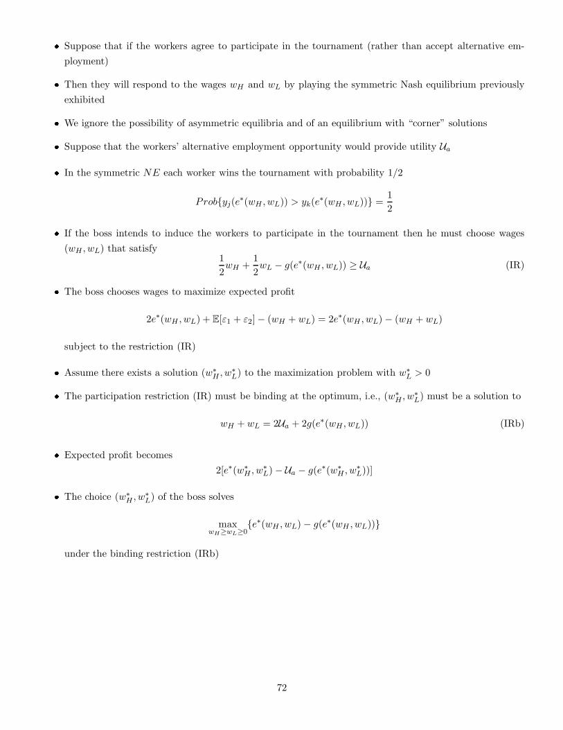
� Suppose that if the workers agree to participate in the tournament (rather than accept alternative em-
ployment)
� Then they will respond to the wages wH and wL by playing the symmetric Nash equilibrium previously
exhibited
� We ignore the possibility of asymmetric equilibria and of an equilibrium with “corner” solutions
� Suppose that the workers’ alternative employment opportunity would provide utility Ua
� In the symmetric NE each worker wins the tournament with probability 1/2
Prob{yj(e∗(wH , wL)) > yk(e∗(wH , wL))} =
1
2
� If the boss intends to induce the workers to participate in the tournament then he must choose wages
(wH , wL) that satisfy1
2wH +
1
2wL − g(e∗(wH , wL)) ≥ Ua (IR)
� The boss chooses wages to maximize expected profit
2e∗(wH , wL) + E[ε1 + ε2]− (wH + wL) = 2e∗(wH , wL)− (wH + wL)
subject to the restriction (IR)
� Assume there exists a solution (w∗H , w∗
L) to the maximization problem with w∗L > 0
� The participation restriction (IR) must be binding at the optimum, i.e., (w∗H , w∗
L) must be a solution to
wH + wL = 2Ua + 2g(e∗(wH , wL)) (IRb)
� Expected profit becomes
2[e∗(w∗H , w∗
L)− Ua − g(e∗(w∗H , w∗
L))]
� The choice (w∗H , w∗
L) of the boss solves
maxwH≥wL≥0
{e∗(wH , wL)− g(e∗(wH , wL))}
under the binding restriction (IRb)
72
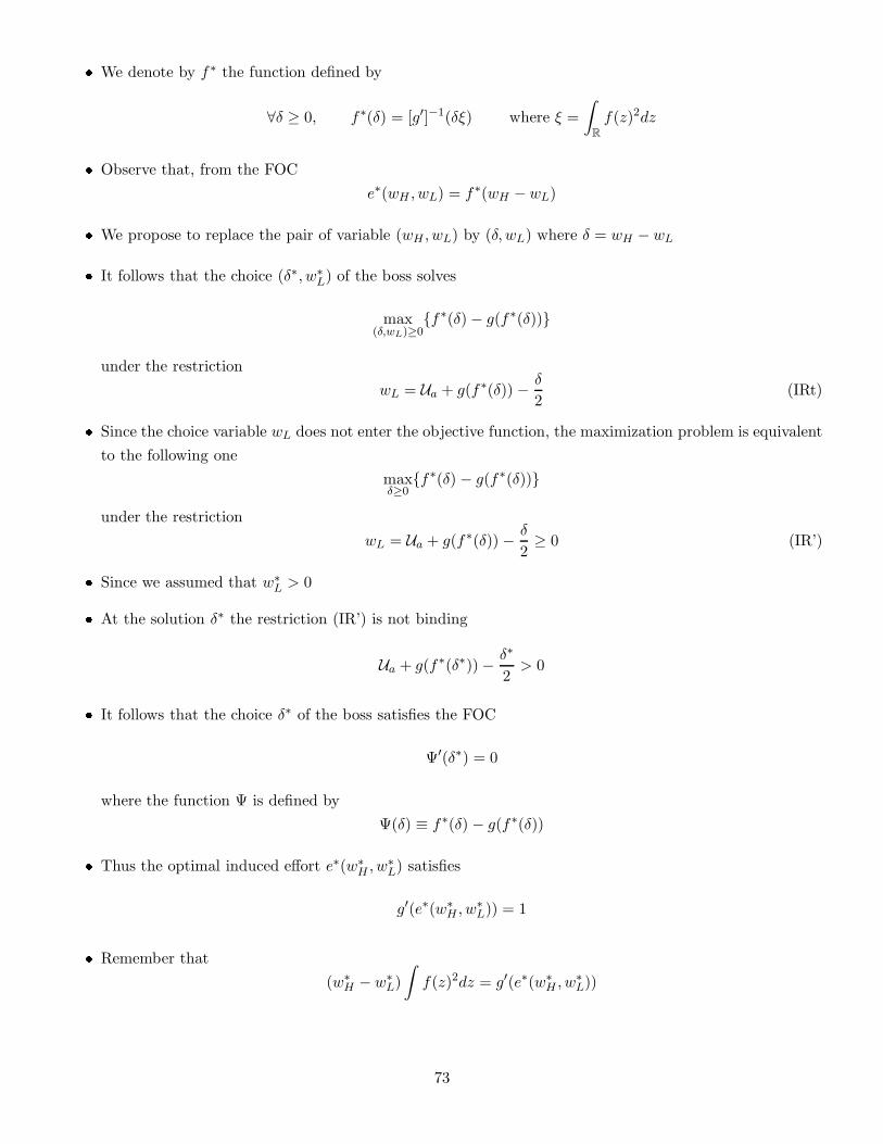
� We denote by f∗ the function defined by
∀δ ≥ 0, f∗(δ) = [g′]−1(δξ) where ξ =
∫
R
f(z)2dz
� Observe that, from the FOC
e∗(wH , wL) = f∗(wH −wL)
� We propose to replace the pair of variable (wH , wL) by (δ, wL) where δ = wH − wL
� It follows that the choice (δ∗, w∗L) of the boss solves
max(δ,wL)≥0
{f∗(δ)− g(f∗(δ))}
under the restriction
wL = Ua + g(f∗(δ)) − δ
2(IRt)
� Since the choice variable wL does not enter the objective function, the maximization problem is equivalent
to the following one
maxδ≥0
{f∗(δ) − g(f∗(δ))}
under the restriction
wL = Ua + g(f∗(δ)) − δ
2≥ 0 (IR’)
� Since we assumed that w∗L > 0
� At the solution δ∗ the restriction (IR’) is not binding
Ua + g(f∗(δ∗))− δ∗
2> 0
� It follows that the choice δ∗ of the boss satisfies the FOC
Ψ′(δ∗) = 0
where the function Ψ is defined by
Ψ(δ) ≡ f∗(δ) − g(f∗(δ))
� Thus the optimal induced effort e∗(w∗H , w∗
L) satisfies
g′(e∗(w∗H , w∗
L)) = 1
� Remember that
(w∗H − w∗
L)
∫
f(z)2dz = g′(e∗(w∗H , w∗
L))
73
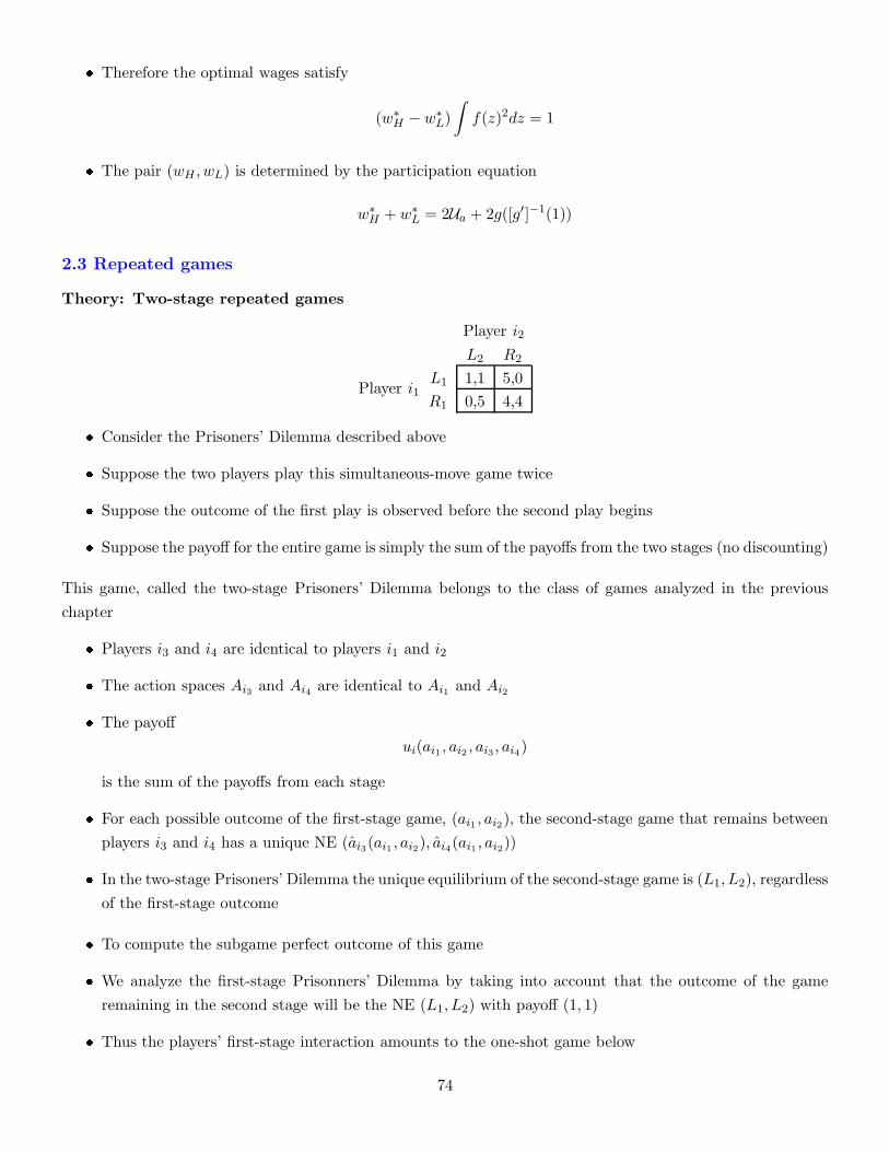
� Therefore the optimal wages satisfy
(w∗H − w∗
L)
∫
f(z)2dz = 1
� The pair (wH , wL) is determined by the participation equation
w∗H + w∗
L = 2Ua + 2g([g′]−1(1))
2.3 Repeated games
Theory: Two-stage repeated games
Player i1
Player i2
L2 R2
L1 1,1 5,0
R1 0,5 4,4
� Consider the Prisoners’ Dilemma described above
� Suppose the two players play this simultaneous-move game twice
� Suppose the outcome of the first play is observed before the second play begins
� Suppose the payoff for the entire game is simply the sum of the payoffs from the two stages (no discounting)
This game, called the two-stage Prisoners’ Dilemma belongs to the class of games analyzed in the previous
chapter
� Players i3 and i4 are identical to players i1 and i2
� The action spaces Ai3 and Ai4 are identical to Ai1 and Ai2
� The payoff
ui(ai1 , ai2 , ai3 , ai4)
is the sum of the payoffs from each stage
� For each possible outcome of the first-stage game, (ai1 , ai2), the second-stage game that remains between
players i3 and i4 has a unique NE (ai3(ai1 , ai2), ai4(ai1 , ai2))
� In the two-stage Prisoners’ Dilemma the unique equilibrium of the second-stage game is (L1, L2), regardless
of the first-stage outcome
� To compute the subgame perfect outcome of this game
� We analyze the first-stage Prisonners’ Dilemma by taking into account that the outcome of the game
remaining in the second stage will be the NE (L1, L2) with payoff (1, 1)
� Thus the players’ first-stage interaction amounts to the one-shot game below
74
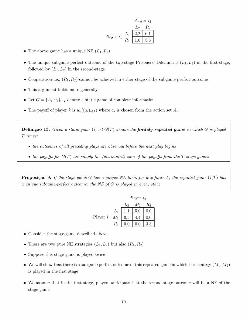
Player i1
Player i2
L2 R2
L1 2,2 6,1
R1 1,6 5,5
� The above game has a unique NE (L1, L2)
� The unique subgame perfect outcome of the two-stage Prisoners’ Dilemma is (L1, L2) in the first-stage,
followed by (L1, L2) in the second-stage
� Cooperation-i.e., (R1, R2)-cannot be achieved in either stage of the subgame perfect outcome
� This argument holds more generally
� Let G = {Ai, ui}i∈I denote a static game of complete information
� The payoff of player k is uk((ai)i∈I) where ai is chosen from the action set Ai
Definicao 15. Given a static game G, let G(T ) denote the finitely repeated game in which G is played
T times:
� the outcomes of all preceding plays are observed before the next play begins
� the payoffs for G(T ) are simply the (discounted) sum of the payoffs from the T stage games
Proposicao 9. If the stage game G has a unique NE then, for any finite T , the repeated game G(T ) has
a unique subgame-perfect outcome: the NE of G is played in every stage
Player i1
Player i2
L2 M2 R2
L1 1,1 5,0 0,0
M1 0,5 4,4 0,0
R1 0,0 0,0 3,3
� Consider the stage-game described above
� There are two pure NE strategies (L1, L2) but also (R1, R2)
� Suppose this stage game is played twice
� We will show that there is a subgame perfect outcome of this repeated game in which the strategy (M1,M2)
is played in the first stage
� We assume that in the first-stage, players anticipate that the second-stage outcome will be a NE of the
stage game
75
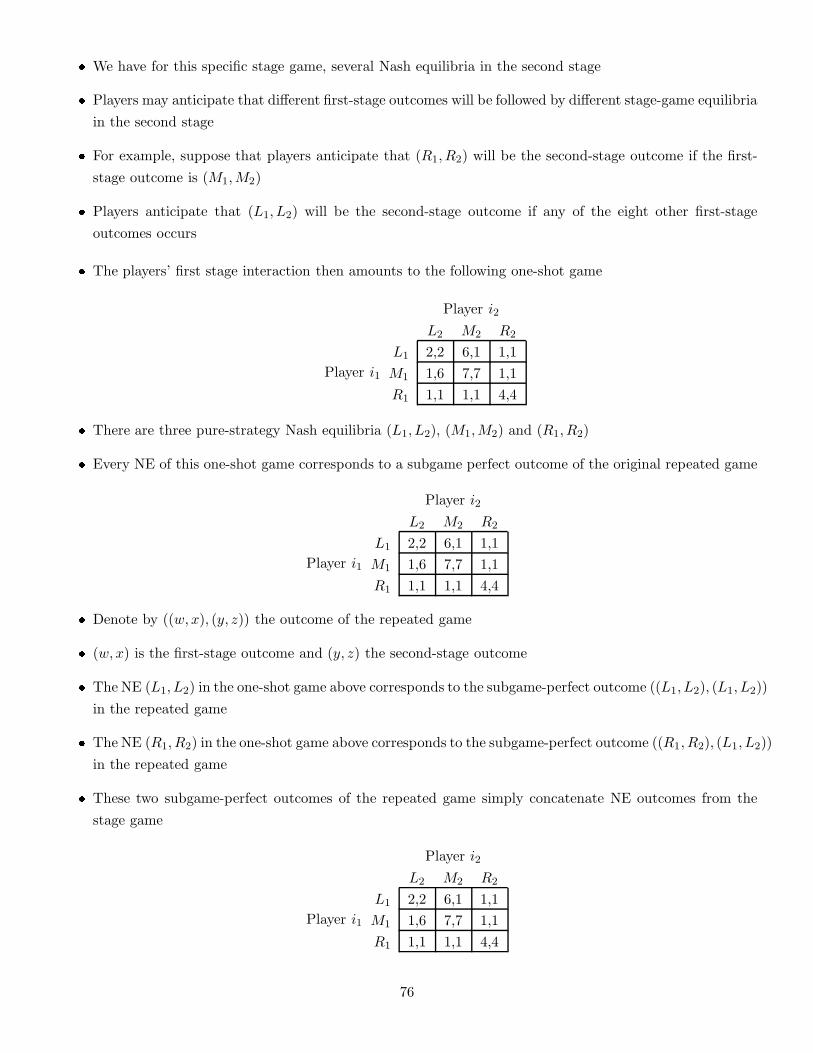
� We have for this specific stage game, several Nash equilibria in the second stage
� Players may anticipate that different first-stage outcomes will be followed by different stage-game equilibria
in the second stage
� For example, suppose that players anticipate that (R1, R2) will be the second-stage outcome if the first-
stage outcome is (M1,M2)
� Players anticipate that (L1, L2) will be the second-stage outcome if any of the eight other first-stage
outcomes occurs
� The players’ first stage interaction then amounts to the following one-shot game
Player i1
Player i2
L2 M2 R2
L1 2,2 6,1 1,1
M1 1,6 7,7 1,1
R1 1,1 1,1 4,4
� There are three pure-strategy Nash equilibria (L1, L2), (M1,M2) and (R1, R2)
� Every NE of this one-shot game corresponds to a subgame perfect outcome of the original repeated game
Player i1
Player i2
L2 M2 R2
L1 2,2 6,1 1,1
M1 1,6 7,7 1,1
R1 1,1 1,1 4,4
� Denote by ((w, x), (y, z)) the outcome of the repeated game
� (w, x) is the first-stage outcome and (y, z) the second-stage outcome
� The NE (L1, L2) in the one-shot game above corresponds to the subgame-perfect outcome ((L1, L2), (L1, L2))
in the repeated game
� The NE (R1, R2) in the one-shot game above corresponds to the subgame-perfect outcome ((R1, R2), (L1, L2))
in the repeated game
� These two subgame-perfect outcomes of the repeated game simply concatenate NE outcomes from the
stage game
Player i1
Player i2
L2 M2 R2
L1 2,2 6,1 1,1
M1 1,6 7,7 1,1
R1 1,1 1,1 4,4
76
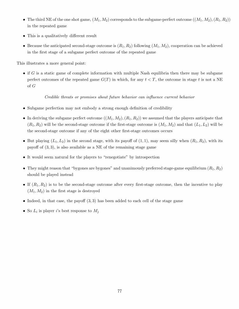
� The third NE of the one shot game, (M1,M2) corresponds to the subgame-perfect outcome ((M1,M2), (R1, R2))
in the repeated game
� This is a qualitatively different result
� Because the anticipated second-stage outcome is (R1, R2) following (M1,M2), cooperation can be achieved
in the first stage of a subgame perfect outcome of the repeated game
This illustrates a more general point:
� if G is a static game of complete information with multiple Nash equilibria then there may be subgame
perfect outcomes of the repeated game G(T ) in which, for any t < T , the outcome in stage t is not a NE
of G
Credible threats or promises about future behavior can influence current behavior
� Subgame perfection may not embody a strong enough definition of credibility
� In deriving the subgame perfect outcome ((M1,M2), (R1, R2)) we assumed that the players anticipate that
(R1, R2) will be the second-stage outcome if the first-stage outcome is (M1,M2) and that (L1, L2) will be
the second-stage outcome if any of the eight other first-stage outcomes occurs
� But playing (L1, L2) in the second stage, with its payoff of (1, 1), may seem silly when (R1, R2), with its
payoff of (3, 3), is also available as a NE of the remaining stage game
� It would seem natural for the players to “renegotiate” by introspection
� They might reason that “bygones are bygones” and unanimously preferred stage-game equilibrium (R1, R2)
should be played instead
� If (R1, R2) is to be the second-stage outcome after every first-stage outcome, then the incentive to play
(M1,M2) in the first stage is destroyed
� Indeed, in that case, the payoff (3, 3) has been added to each cell of the stage game
� So Li is player i’s best response to Mj
77
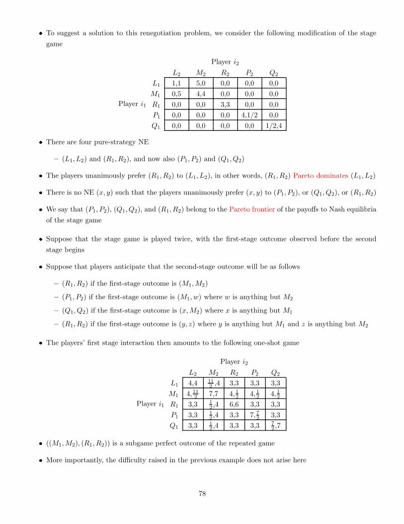
� To suggest a solution to this renegotiation problem, we consider the following modification of the stage
game
Player i1
Player i2
L2 M2 R2 P2 Q2
L1 1,1 5,0 0,0 0,0 0,0
M1 0,5 4,4 0,0 0,0 0,0
R1 0,0 0,0 3,3 0,0 0,0
P1 0,0 0,0 0,0 4,1/2 0,0
Q1 0,0 0,0 0,0 0,0 1/2,4
� There are four pure-strategy NE
– (L1, L2) and (R1, R2), and now also (P1, P2) and (Q1, Q2)
� The players unanimously prefer (R1, R2) to (L1, L2), in other words, (R1, R2) Pareto dominates (L1, L2)
� There is no NE (x, y) such that the players unanimously prefer (x, y) to (P1, P2), or (Q1, Q2), or (R1, R2)
� We say that (P1, P2), (Q1, Q2), and (R1, R2) belong to the Pareto frontier of the payoffs to Nash equilibria
of the stage game
� Suppose that the stage game is played twice, with the first-stage outcome observed before the second
stage begins
� Suppose that players anticipate that the second-stage outcome will be as follows
– (R1, R2) if the first-stage outcome is (M1,M2)
– (P1, P2) if the first-stage outcome is (M1, w) where w is anything but M2
– (Q1, Q2) if the first-stage outcome is (x,M2) where x is anything but M1
– (R1, R2) if the first-stage outcome is (y, z) where y is anything but M1 and z is anything but M2
� The players’ first stage interaction then amounts to the following one-shot game
Player i1
Player i2
L2 M2 R2 P2 Q2
L1 4,4 112 ,4 3,3 3,3 3,3
M1 4,112 7,7 4,12 4,12 4,12R1 3,3 1
2 ,4 6,6 3,3 3,3
P1 3,3 12 ,4 3,3 7,72 3,3
Q1 3,3 12 ,4 3,3 3,3 7
2 ,7
� ((M1,M2), (R1, R2)) is a subgame perfect outcome of the repeated game
� More importantly, the difficulty raised in the previous example does not arise here
78
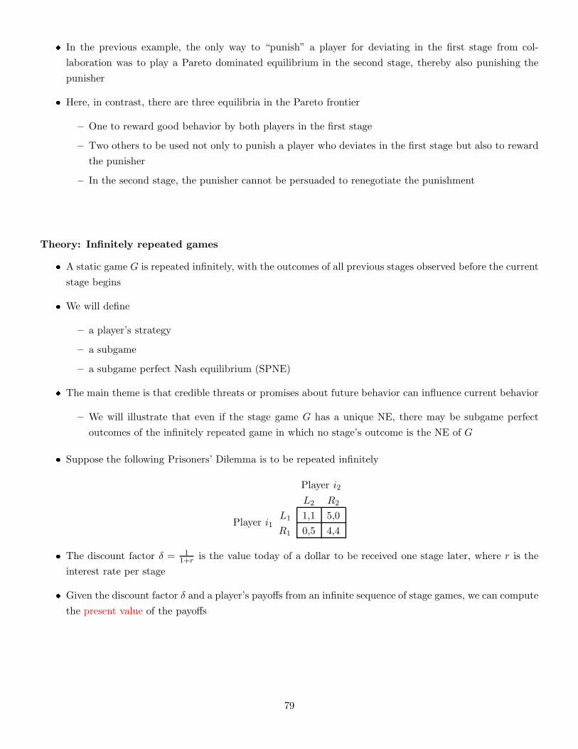
� In the previous example, the only way to “punish” a player for deviating in the first stage from col-
laboration was to play a Pareto dominated equilibrium in the second stage, thereby also punishing the
punisher
� Here, in contrast, there are three equilibria in the Pareto frontier
– One to reward good behavior by both players in the first stage
– Two others to be used not only to punish a player who deviates in the first stage but also to reward
the punisher
– In the second stage, the punisher cannot be persuaded to renegotiate the punishment
Theory: Infinitely repeated games
� A static game G is repeated infinitely, with the outcomes of all previous stages observed before the current
stage begins
� We will define
– a player’s strategy
– a subgame
– a subgame perfect Nash equilibrium (SPNE)
� The main theme is that credible threats or promises about future behavior can influence current behavior
– We will illustrate that even if the stage game G has a unique NE, there may be subgame perfect
outcomes of the infinitely repeated game in which no stage’s outcome is the NE of G
� Suppose the following Prisoners’ Dilemma is to be repeated infinitely
Player i1
Player i2
L2 R2
L1 1,1 5,0
R1 0,5 4,4
� The discount factor δ = 11+r
is the value today of a dollar to be received one stage later, where r is the
interest rate per stage
� Given the discount factor δ and a player’s payoffs from an infinite sequence of stage games, we can compute
the present value of the payoffs
79
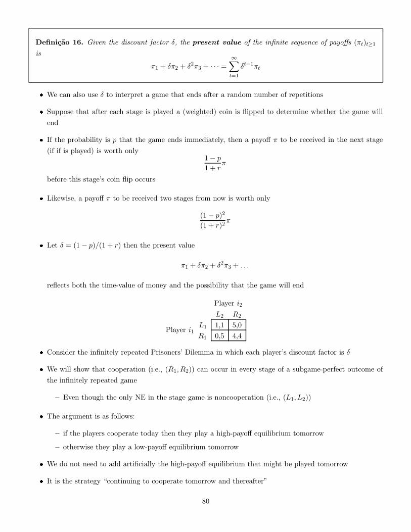
Definicao 16. Given the discount factor δ, the present value of the infinite sequence of payoffs (πt)t≥1
is
π1 + δπ2 + δ2π3 + · · · =∞∑
t=1
δt−1πt
� We can also use δ to interpret a game that ends after a random number of repetitions
� Suppose that after each stage is played a (weighted) coin is flipped to determine whether the game will
end
� If the probability is p that the game ends immediately, then a payoff π to be received in the next stage
(if if is played) is worth only1− p
1 + rπ
before this stage’s coin flip occurs
� Likewise, a payoff π to be received two stages from now is worth only
(1− p)2
(1 + r)2π
� Let δ = (1− p)/(1 + r) then the present value
π1 + δπ2 + δ2π3 + . . .
reflects both the time-value of money and the possibility that the game will end
Player i1
Player i2
L2 R2
L1 1,1 5,0
R1 0,5 4,4
� Consider the infinitely repeated Prisoners’ Dilemma in which each player’s discount factor is δ
� We will show that cooperation (i.e., (R1, R2)) can occur in every stage of a subgame-perfect outcome of
the infinitely repeated game
– Even though the only NE in the stage game is noncooperation (i.e., (L1, L2))
� The argument is as follows:
– if the players cooperate today then they play a high-payoff equilibrium tomorrow
– otherwise they play a low-payoff equilibrium tomorrow
� We do not need to add artificially the high-payoff equilibrium that might be played tomorrow
� It is the strategy “continuing to cooperate tomorrow and thereafter”
80
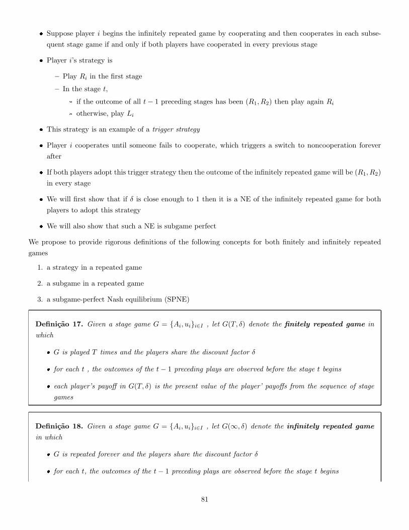
� Suppose player i begins the infinitely repeated game by cooperating and then cooperates in each subse-
quent stage game if and only if both players have cooperated in every previous stage
� Player i’s strategy is
– Play Ri in the first stage
– In the stage t,
* if the outcome of all t− 1 preceding stages has been (R1, R2) then play again Ri
* otherwise, play Li
� This strategy is an example of a trigger strategy
� Player i cooperates until someone fails to cooperate, which triggers a switch to noncooperation forever
after
� If both players adopt this trigger strategy then the outcome of the infinitely repeated game will be (R1, R2)
in every stage
� We will first show that if δ is close enough to 1 then it is a NE of the infinitely repeated game for both
players to adopt this strategy
� We will also show that such a NE is subgame perfect
We propose to provide rigorous definitions of the following concepts for both finitely and infinitely repeated
games
1. a strategy in a repeated game
2. a subgame in a repeated game
3. a subgame-perfect Nash equilibrium (SPNE)
Definicao 17. Given a stage game G = {Ai, ui}i∈I , let G(T, δ) denote the finitely repeated game in
which
� G is played T times and the players share the discount factor δ
� for each t , the outcomes of the t− 1 preceding plays are observed before the stage t begins
� each player’s payoff in G(T, δ) is the present value of the player’ payoffs from the sequence of stage
games
Definicao 18. Given a stage game G = {Ai, ui}i∈I , let G(∞, δ) denote the infinitely repeated game
in which
� G is repeated forever and the players share the discount factor δ
� for each t, the outcomes of the t− 1 preceding plays are observed before the stage t begins
81
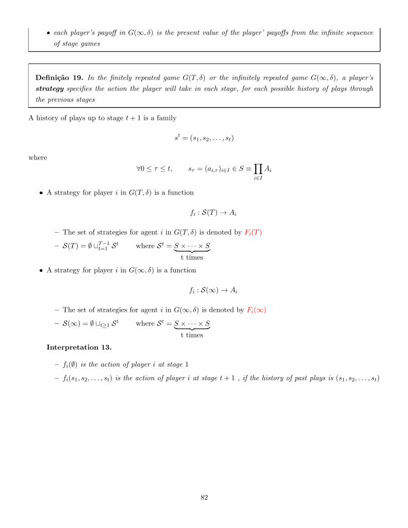
� each player’s payoff in G(∞, δ) is the present value of the player’ payoffs from the infinite sequence
of stage games
Definicao 19. In the finitely repeated game G(T, δ) or the infinitely repeated game G(∞, δ), a player’s
strategy specifies the action the player will take in each stage, for each possible history of plays through
the previous stages
A history of plays up to stage t+ 1 is a family
st = (s1, s2, . . . , st)
where
∀0 ≤ τ ≤ t, sτ = (ai,τ )i∈I ∈ S ≡∏
i∈I
Ai
� A strategy for player i in G(T, δ) is a function
fi : S(T ) → Ai
– The set of strategies for agent i in G(T, δ) is denoted by Fi(T )
– S(T ) = ∅ ∪T−1t=1 St where St = S × · · · × S
︸ ︷︷ ︸
t times
� A strategy for player i in G(∞, δ) is a function
fi : S(∞) → Ai
– The set of strategies for agent i in G(∞, δ) is denoted by Fi(∞)
– S(∞) = ∅ ∪t≥1 St where St = S × · · · × S︸ ︷︷ ︸
t times
Interpretation 13.
– fi(∅) is the action of player i at stage 1
– fi(s1, s2, . . . , st) is the action of player i at stage t+ 1 , if the history of past plays is (s1, s2, . . . , st)
82
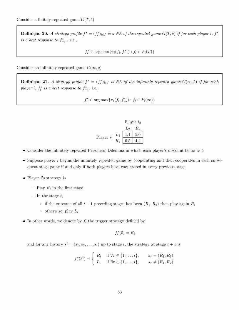
Consider a finitely repeated game G(T, δ)
Definicao 20. A strategy profile f∗ = (f∗i )i∈I is a NE of the repeated game G(T, δ) if for each player i, f∗
i
is a best response to f∗−i , i.e.,
f∗i ∈ argmax{πi(fi, f∗
−i) : fi ∈ Fi(T )}
Consider an infinitely repeated game G(∞, δ)
Definicao 21. A strategy profile f∗ = (f∗i )i∈I is NE of the infinitely repeated game G(∞, δ) if for each
player i, f∗i is a best response to f∗
−i, i.e.,
f∗i ∈ argmax{πi(fi, f∗
−i) : fi ∈ Fi(∞)}
Player i1
Player i2
L2 R2
L1 1,1 5,0
R1 0,5 4,4
� Consider the infinitely repeated Prisoners’ Dilemma in which each player’s discount factor is δ
� Suppose player i begins the infinitely repeated game by cooperating and then cooperates in each subse-
quent stage game if and only if both players have cooperated in every previous stage
� Player i’s strategy is
– Play Ri in the first stage
– In the stage t,
* if the outcome of all t− 1 preceding stages has been (R1, R2) then play again Ri
* otherwise, play Li
� In other words, we denote by fi the trigger strategy defined by
f∗i (∅) = Ri
and for any history st = (s1, s2, . . . , st) up to stage t, the strategy at stage t+ 1 is
f∗i (s
t) =
{
Ri if ∀τ ∈ {1, . . . , t}, sτ = (R1, R2)
Li if ∃τ ∈ {1, . . . , t}, sτ 6= (R1, R2)
83
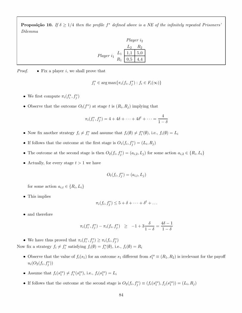
Proposicao 10. If δ ≥ 1/4 then the profile f∗ defined above is a NE of the infinitely repeated Prisoners’
Dilemma
Player i1
Player i2
L2 R2
L1 1,1 5,0
R1 0,5 4,4
Proof. � Fix a player i, we shall prove that
f∗i ∈ argmax{πi(fi, f∗
j ) : fi ∈ Fi(∞)}
� We first compute πi(f∗i , f
∗j )
� Observe that the outcome Ot(f∗) at stage t is (Ri, Rj) implying that
πi(f∗i , f
∗j ) = 4 + 4δ + · · ·+ 4δt + · · · = 4
1− δ
� Now fix another strategy fi 6= f∗i and assume that fi(∅) 6= f∗
i (∅), i.e., fi(∅) = Li
� If follows that the outcome at the first stage is O1(fi, f∗j ) = (Li, Rj)
� The outcome at the second stage is then O2(fi, f∗j ) = (ai,2, Lj) for some action ai,2 ∈ {Ri, Li}
� Actually, for every stage t > 1 we have
Ot(fi, f∗j ) = (ai,t, Lj)
for some action ai,t ∈ {Ri, Li}
� This implies
πi(fi, f∗j ) ≤ 5 + δ + · · ·+ δt + . . .
� and therefore
πi(f∗i , f
∗j )− πi(fi, f
∗j ) ≥ −1 + 3
δ
1− δ=
4δ − 1
1− δ
� We have thus proved that πi(f∗i , f
∗j ) ≥ πi(fi, f
∗j )
Now fix a strategy fi 6= f∗i satisfying fi(∅) = f∗
i (∅), i.e., fi(∅) = Ri
� Observe that the value of fi(s1) for an outcome s1 different from sco1 ≡ (R1, R2) is irrelevant for the payoff
ui(O2(fi, f∗j ))
� Assume that fi(sco1 ) 6= f∗
i (sco1 ), i.e., fi(s
co1 ) = Li
� If follows that the outcome at the second stage is O2(fi, f∗j ) ≡ (fi(s
co1 ), fj(s
co1 )) = (Li, Rj)
84
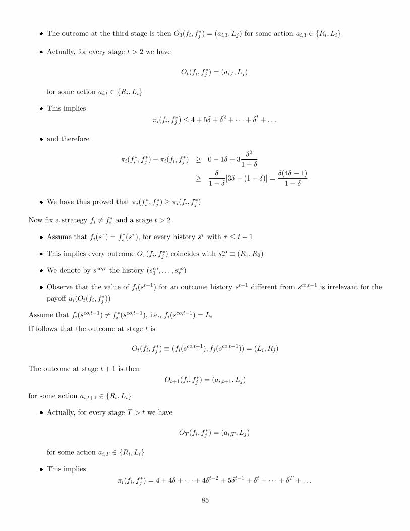
� The outcome at the third stage is then O3(fi, f∗j ) = (ai,3, Lj) for some action ai,3 ∈ {Ri, Li}
� Actually, for every stage t > 2 we have
Ot(fi, f∗j ) = (ai,t, Lj)
for some action ai,t ∈ {Ri, Li}
� This implies
πi(fi, f∗j ) ≤ 4 + 5δ + δ2 + · · ·+ δt + . . .
� and therefore
πi(f∗i , f
∗j )− πi(fi, f
∗j ) ≥ 0− 1δ + 3
δ2
1− δ
≥ δ
1− δ[3δ − (1− δ)] =
δ(4δ − 1)
1− δ
� We have thus proved that πi(f∗i , f
∗j ) ≥ πi(fi, f
∗j )
Now fix a strategy fi 6= f∗i and a stage t > 2
� Assume that fi(sτ ) = f∗
i (sτ ), for every history sτ with τ ≤ t− 1
� This implies every outcome Oτ (fi, f∗j ) coincides with scoτ ≡ (R1, R2)
� We denote by sco,τ the history (sco1 , . . . , scoτ )
� Observe that the value of fi(st−1) for an outcome history st−1 different from sco,t−1 is irrelevant for the
payoff ui(Ot(fi, f∗j ))
Assume that fi(sco,t−1) 6= f∗
i (sco,t−1), i.e., fi(s
co,t−1) = Li
If follows that the outcome at stage t is
Ot(fi, f∗j ) ≡ (fi(s
co,t−1), fj(sco,t−1)) = (Li, Rj)
The outcome at stage t+ 1 is then
Ot+1(fi, f∗j ) = (ai,t+1, Lj)
for some action ai,t+1 ∈ {Ri, Li}
� Actually, for every stage T > t we have
OT (fi, f∗j ) = (ai,T , Lj)
for some action ai,T ∈ {Ri, Li}
� This implies
πi(fi, f∗j ) = 4 + 4δ + · · ·+ 4δt−2 + 5δt−1 + δt + · · ·+ δT + . . .
85
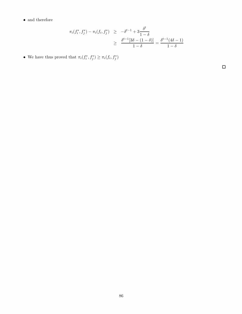
� and therefore
πi(f∗i , f
∗j )− πi(fi, f
∗j ) ≥ −δt−1 + 3
δt
1− δ
≥ δt−1[3δ − (1− δ)]
1− δ=
δt−1(4δ − 1)
1− δ
� We have thus proved that πi(f∗i , f
∗j ) ≥ πi(fi, f
∗j )
86
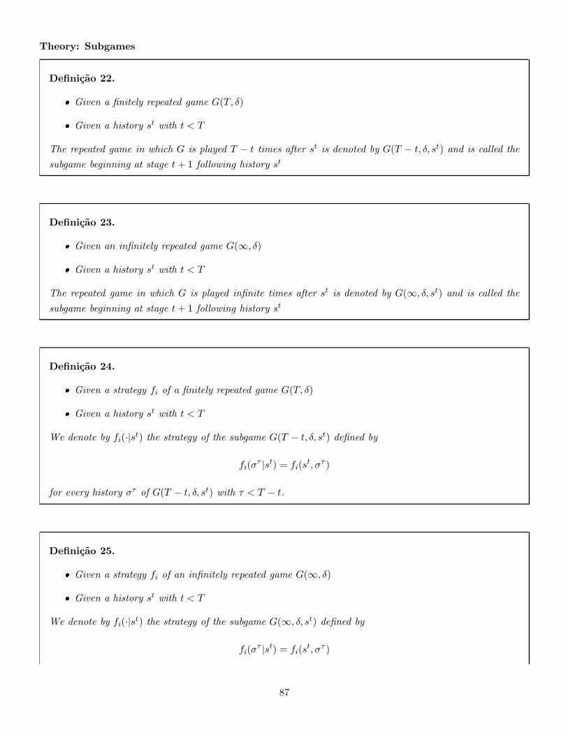
Theory: Subgames
Definicao 22.
� Given a finitely repeated game G(T, δ)
� Given a history st with t < T
The repeated game in which G is played T − t times after st is denoted by G(T − t, δ, st) and is called the
subgame beginning at stage t+ 1 following history st
Definicao 23.
� Given an infinitely repeated game G(∞, δ)
� Given a history st with t < T
The repeated game in which G is played infinite times after st is denoted by G(∞, δ, st) and is called the
subgame beginning at stage t+ 1 following history st
Definicao 24.
� Given a strategy fi of a finitely repeated game G(T, δ)
� Given a history st with t < T
We denote by fi(·|st) the strategy of the subgame G(T − t, δ, st) defined by
fi(στ |st) = fi(s
t, στ )
for every history στ of G(T − t, δ, st) with τ < T − t.
Definicao 25.
� Given a strategy fi of an infinitely repeated game G(∞, δ)
� Given a history st with t < T
We denote by fi(·|st) the strategy of the subgame G(∞, δ, st) defined by
fi(στ |st) = fi(s
t, στ )
87
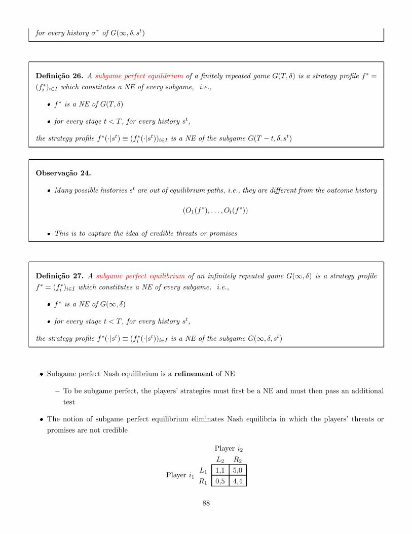
for every history στ of G(∞, δ, st)
Definicao 26. A subgame perfect equilibrium of a finitely repeated game G(T, δ) is a strategy profile f∗ =
(f∗i )i∈I which constitutes a NE of every subgame, i.e.,
� f∗ is a NE of G(T, δ)
� for every stage t < T , for every history st,
the strategy profile f∗(·|st) ≡ (f∗i (·|st))i∈I is a NE of the subgame G(T − t, δ, st)
Observacao 24.
� Many possible histories st are out of equilibrium paths, i.e., they are different from the outcome history
(O1(f∗), . . . , Ot(f
∗))
� This is to capture the idea of credible threats or promises
Definicao 27. A subgame perfect equilibrium of an infinitely repeated game G(∞, δ) is a strategy profile
f∗ = (f∗i )i∈I which constitutes a NE of every subgame, i.e.,
� f∗ is a NE of G(∞, δ)
� for every stage t < T , for every history st,
the strategy profile f∗(·|st) ≡ (f∗i (·|st))i∈I is a NE of the subgame G(∞, δ, st)
� Subgame perfect Nash equilibrium is a refinement of NE
– To be subgame perfect, the players’ strategies must first be a NE and must then pass an additional
test
� The notion of subgame perfect equilibrium eliminates Nash equilibria in which the players’ threats or
promises are not credible
Player i1
Player i2
L2 R2
L1 1,1 5,0
R1 0,5 4,4
88
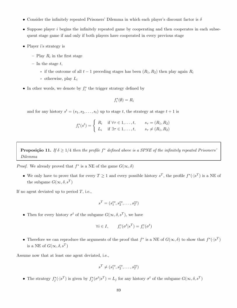
� Consider the infinitely repeated Prisoners’ Dilemma in which each player’s discount factor is δ
� Suppose player i begins the infinitely repeated game by cooperating and then cooperates in each subse-
quent stage game if and only if both players have cooperated in every previous stage
� Player i’s strategy is
– Play Ri in the first stage
– In the stage t,
* if the outcome of all t− 1 preceding stages has been (R1, R2) then play again Ri
* otherwise, play Li
� In other words, we denote by f∗i the trigger strategy defined by
f∗i (∅) = Ri
and for any history st = (s1, s2, . . . , st) up to stage t, the strategy at stage t+ 1 is
f∗i (s
t) =
{
Ri if ∀τ ∈ 1, . . . , t, sτ = (R1, R2)
Li if ∃τ ∈ 1, . . . , t, sτ 6= (R1, R2)
Proposicao 11. If δ ≥ 1/4 then the profile f∗ defined above is a SPNE of the infinitely repeated Prisoners’
Dilemma
Proof. We already proved that f∗ is a NE of the game G(∞, δ)
� We only have to prove that for every T ≥ 1 and every possible history sT , the profile f∗(·|sT ) is a NE of
the subgame G(∞, δ, sT )
If no agent deviated up to period T , i.e.,
sT = (sco1 , sco2 , . . . , scoT )
� Then for every history σt of the subgame G(∞, δ, sT ), we have
∀i ∈ I, f∗i (σ
t|sT ) = f∗i (σ
t)
� Therefore we can reproduce the arguments of the proof that f∗ is a NE of G(∞, δ) to show that f∗(·|sT )is a NE of G(∞, δ, sT )
Assume now that at least one agent deviated, i.e.,
sT 6= (sco1 , sco2 , . . . , scoT )
� The strategy f∗j (·|sT ) is given by f∗
j (σt|sT ) = Lj for any history σt of the subgame G(∞, δ, sT )
89
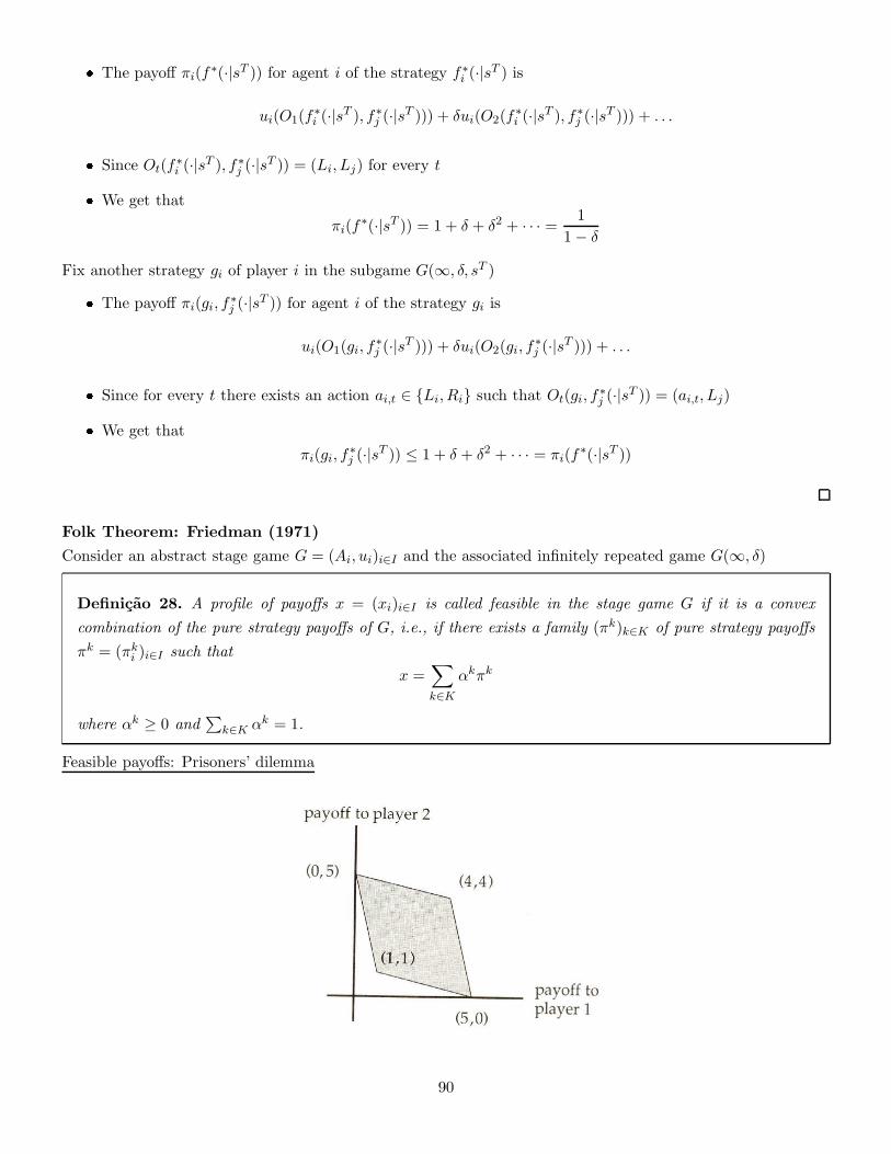
� The payoff πi(f∗(·|sT )) for agent i of the strategy f∗
i (·|sT ) is
ui(O1(f∗i (·|sT ), f∗
j (·|sT ))) + δui(O2(f∗i (·|sT ), f∗
j (·|sT ))) + . . .
� Since Ot(f∗i (·|sT ), f∗
j (·|sT )) = (Li, Lj) for every t
� We get that
πi(f∗(·|sT )) = 1 + δ + δ2 + · · · = 1
1− δ
Fix another strategy gi of player i in the subgame G(∞, δ, sT )
� The payoff πi(gi, f∗j (·|sT )) for agent i of the strategy gi is
ui(O1(gi, f∗j (·|sT ))) + δui(O2(gi, f
∗j (·|sT ))) + . . .
� Since for every t there exists an action ai,t ∈ {Li, Ri} such that Ot(gi, f∗j (·|sT )) = (ai,t, Lj)
� We get that
πi(gi, f∗j (·|sT )) ≤ 1 + δ + δ2 + · · · = πi(f
∗(·|sT ))
Folk Theorem: Friedman (1971)
Consider an abstract stage game G = (Ai, ui)i∈I and the associated infinitely repeated game G(∞, δ)
Definicao 28. A profile of payoffs x = (xi)i∈I is called feasible in the stage game G if it is a convex
combination of the pure strategy payoffs of G, i.e., if there exists a family (πk)k∈K of pure strategy payoffs
πk = (πki )i∈I such that
x =∑
k∈K
αkπk
where αk ≥ 0 and∑
k∈K αk = 1.
Feasible payoffs: Prisoners’ dilemma
90
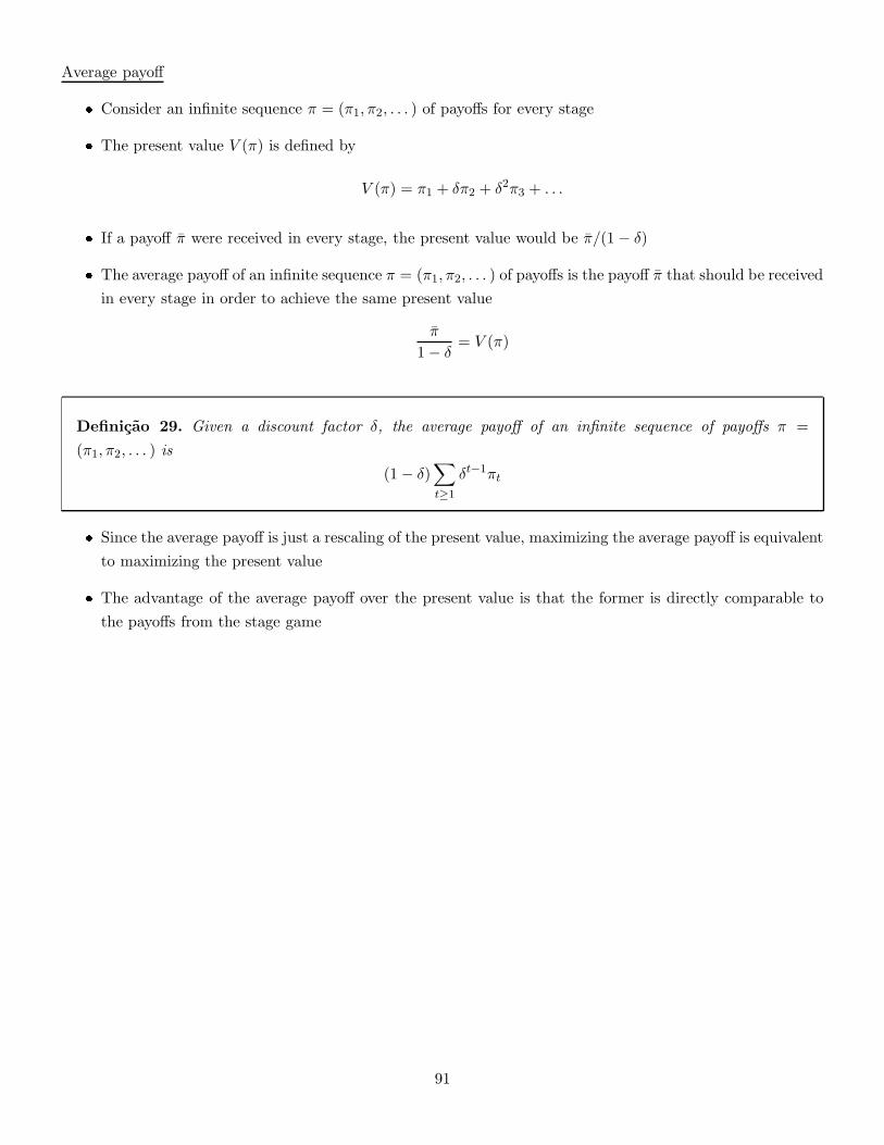
Average payoff
� Consider an infinite sequence π = (π1, π2, . . . ) of payoffs for every stage
� The present value V (π) is defined by
V (π) = π1 + δπ2 + δ2π3 + . . .
� If a payoff π were received in every stage, the present value would be π/(1− δ)
� The average payoff of an infinite sequence π = (π1, π2, . . . ) of payoffs is the payoff π that should be received
in every stage in order to achieve the same present value
π
1− δ= V (π)
Definicao 29. Given a discount factor δ, the average payoff of an infinite sequence of payoffs π =
(π1, π2, . . . ) is
(1− δ)∑
t≥1
δt−1πt
� Since the average payoff is just a rescaling of the present value, maximizing the average payoff is equivalent
to maximizing the present value
� The advantage of the average payoff over the present value is that the former is directly comparable to
the payoffs from the stage game
91
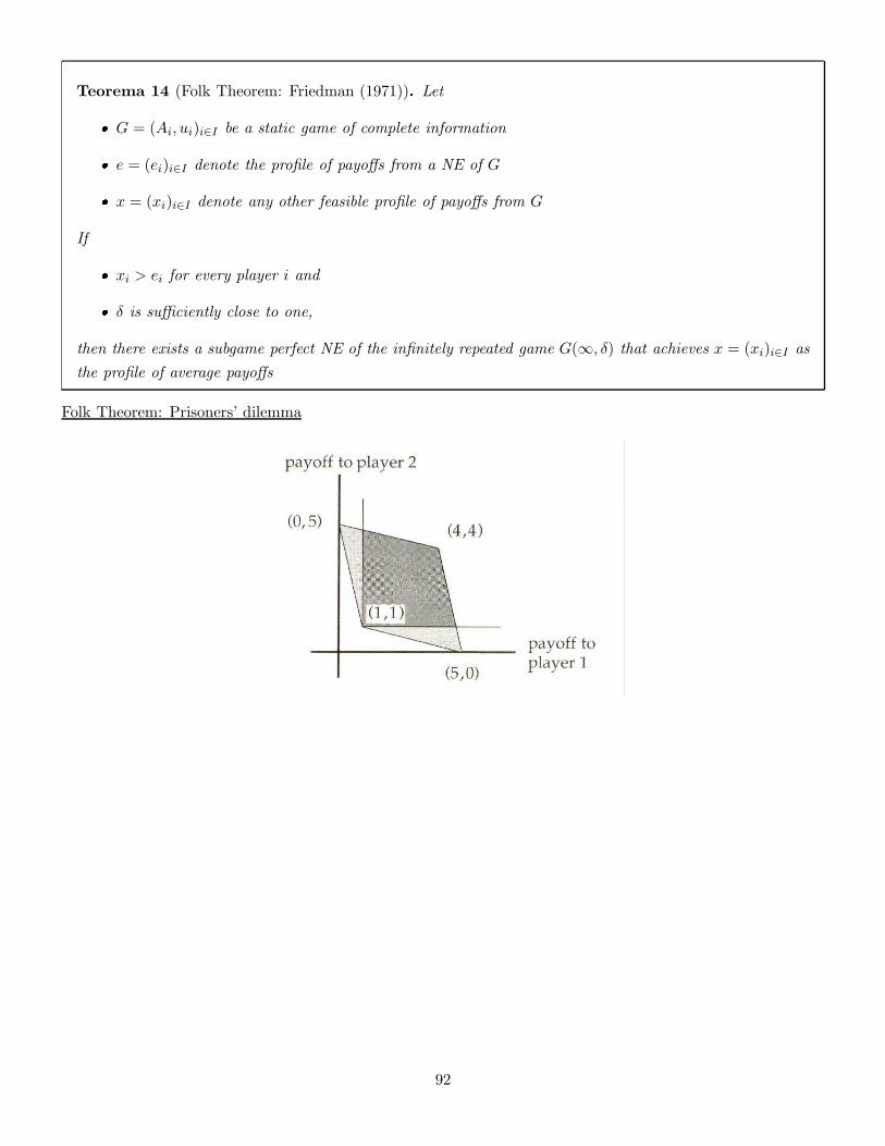
Teorema 14 (Folk Theorem: Friedman (1971)). Let
� G = (Ai, ui)i∈I be a static game of complete information
� e = (ei)i∈I denote the profile of payoffs from a NE of G
� x = (xi)i∈I denote any other feasible profile of payoffs from G
If
� xi > ei for every player i and
� δ is sufficiently close to one,
then there exists a subgame perfect NE of the infinitely repeated game G(∞, δ) that achieves x = (xi)i∈I as
the profile of average payoffs
Folk Theorem: Prisoners’ dilemma
92
Collusion between Cournot duopolists
Cournot duopoly
� Recall the static Cournot game
� If the aggregate quantity on the market is Q = qi1 + qi2
� Then the market clearing price is P (Q) = [a−Q]+
� Each firm has a marginal cost of c > 0 and no fixed costs
� Firms choose quantities simultaneously
� In the unique NE, each firm produces the quantity (a− c)/3
� This quantity is called the Cournot quantity and is denoted by qC
� The equilibrium aggregate quantity, 2(a− c)/3 exceeds the monopoly quantity, qm ≡ (a− c)/2
� Both firms would be better off if each produced half the monopoly quantity, qi = qm/2
Infinitely repeated Cournot duopoly
� Consider the infinitely repeated game based on this Cournot stage game when both firms have the dis-
counted factor δ
� Consider the following trigger strategy for each firm
– Produce half the monopoly quantity, qm/2, in the first period
– In stage t,
* produce qm/2 if both firms have produced qm/2 in each of the t− 1 previous stages;
* otherwise, produce the Cournot quantity, qC
� We propose to compute the values of δ for which it is a subgame perfect Nash equilibrium to play the
previous trigger strategy
� The profit to one firm when both produce qm/2 is (a− c)2/8, which will be denoted by πm/2
� The profit to one firm when both produce qC is (a− c)2/9, which will be denoted by πC
� If firm i is going to produce qm/2 this period then the quantity that maximizes firm j’s profit this period
solves
argmax{[a− c− qj − (qm/2)]qj : qj ≥ 0}
� The solution is qj = 3(a− c)/8, with associated profit of πd ≡ 9(a− c)2/64
� It is a NE for both firms to play the trigger strategy when
1
1− δ× πm
2≥ πd +
δ
1− δπC
93
� This yields δ ≥ 9/17
� For the same reasons as the Prisoners’ Dilemma infinitely repeated game, this NE is subgame perfect
� We propose to study what the firms can achieve if δ < 9/17
� We first determine, for a given value of δ, the most profitable quantity the firms can produce if they both
play trigger strategies that switch forever to the Cournot quantity after any deviation
� We know that such trigger strategies cannot support a quantity as low as qm/2
� But for any value of δ it is a SPNE simply to repeat the Cournot quantity forever
� This implies that the most profitable quantity that triggers strategies can support is between qm/2 and
qC
� Consider the following trigger strategy
– Produce q∗ in the first period
– In the stage t,
* produce q∗ if both firms have produced q∗ in each of t− 1 previous periods;
* otherwise, produce the Cournot quantity, qC
� The profit of one firm if both play q∗ is π∗ ≡ (a− c− 2q∗)q∗
� If firm i is going to produce q∗ this period, then the quantity that maximizes firm j’s profit this period
solves
argmax{(a− c− qj − q∗)qj : qj ≥ 0}
� The solution is qj = (a− c− q∗)/2 with associated profit
πd ≡ (a− c− q∗)2
4
� It is a NE for both firms to play the trigger strategy given before provided that
1
1− δπ∗ ≥ πd +
δ
1− δπC
� Solving the resulting quadratic in q∗ shows that the lowest value of q∗ for which the trigger strategies are
a SPNE is
q∗(δ) =9− 5δ
3(9 − δ)(a− c)
� The function δ 7→ q∗(δ) is decreasing and satisfies
limδ→ 9
17
q∗(δ) =qm2
and limδ→0
q∗(δ) = qC
94
� We now explore the second approach, which involves threatening to administer the strongest credible
punishment
� We propose to show that Abreu’s approach can achieve the monopoly outcome in our model when δ = 1/2
(which is less than 9/17)
� Consider the following “two phase” strategy
– Produce half the monopoly quantity, qm/2, in the first period
– In stage t,
* produce qm/2 if both firms produced qm/2 in period t− 1
* produce qm/2 if both firms produced x in period t− 1
* Otherwise produce x
� This strategy involves a one-period punishment phase
� And a (potentially infinite) collusive phase in which the firm produces qm/2
� The profit to one firm if both produce x is π(x) ≡ (a− c− 2x)x
� Let V (x) denote the present value of receiving π(x) this period and half the monopoly profit forever after:
V (x) = π(x) +δ
1− δ× πm
2
� If firm i is going to produce x this period, then the quantity that maximizes firm j’s profit this period
solves
argmax{(a− c− qj − x)qj : qj ≥ 0}
� The solution is qj = (a− c− x)/2, with associated profit
πdp(x) ≡(a− c− x)2
4
Teorema 15. The “two-phase” strategy is a SPNE if and only if
1
1− δ× 1
2πm ≥ πd + δV (x) (1)
and
V (x) ≥ πdp(x) + δV (x) (2)
� For δ = 1/2, condition (3) is satisfied provided
x
a− c/∈[1
8,3
8
]
95
� For δ = 1/2, condition (4) is satisfied provided
x
a− c∈[3
10,1
2
]
� For δ = 1/2, the two-phase strategy achieves the monopoly outcome as a SPNE provided that
x
a− c∈[3
8,1
2
]
2.4 Dynamic games of complete but imperfect information
Extensive-form representation of games
Extensive-form representation
� It may seem that that static games must be represented in normal form and dynamic games in extensive
form
– This is not the case
� Any game can be represented in either normal or extensive form
� Although for some games one of the two forms is more convenient to analyze
� We will discuss how static games can be represented using extensive form and how dynamic games can
be represented using normal form
Normal-form representation
The normal-form representation of a game specifies
1. the players in the game
2. the strategies available to each player
3. the payoff received by each player for each combination of strategies that could be chosen by the players
Definicao 30. The extensive-form representation of a game specifies
1. the players in the game
2. (a) when each player has the move
(b) what each player can do at each of his or her opportunities to move
(c) what each player knows at each of his or her opportunities to move
96
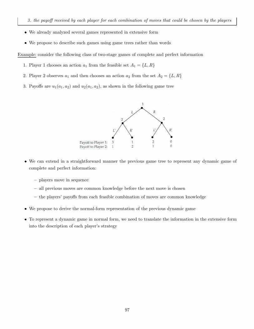
3. the payoff received by each player for each combination of moves that could be chosen by the players
� We already analyzed several games represented in extensive form
� We propose to describe such games using game trees rather than words
Example: consider the following class of two-stage games of complete and perfect information
1. Player 1 chooses an action a1 from the feasible set A1 = {L,R}
2. Player 2 observes a1 and then chooses an action a2 from the set A2 = {L,R}
3. Payoffs are u1(a1, a2) and u2(a1, a2), as shown in the following game tree
� We can extend in a straightforward manner the previous game tree to represent any dynamic game of
complete and perfect information:
– players move in sequence
– all previous moves are common knowledge before the next move is chosen
– the players’ payoffs from each feasible combination of moves are common knowledge
� We propose to derive the normal-form representation of the previous dynamic game
� To represent a dynamic game in normal form, we need to translate the information in the extensive form
into the description of each player’s strategy
97
Normal-form representation of dynamic games
Definicao 31. A strategy for a player is a complete plan of action: it specifies a feasible action for the
player in every contingency in which the player might be called on to act
� We could not apply the notion of Nash equilibrium to dynamic games of complete information if we
allowed a player’s strategy to leave the actions in some contingencies unspecified
� For player j to compute a best response to payer i’s strategy, j may need to consider how i would act in
every contingency, not just in the contingencies i thinks likely to arise
� In the previous game, player 2 has two actions but four strategies
� This is because there are two contingencies
Strategies of player 2:
Strategy 1 If player 1 plays L then play L′, if player 1 plays R then play L′
f2(a1) =
{
L′ if a1 = L
L′ if a1 = R
This strategy may be denoted by (L′, L′)
Strategy 2 If player 1 plays L then play L′, if player 1 plays R then play R′
f2(a1) =
{
L′ if a1 = L
R′ if a1 = R
This strategy may be denoted by (L′, R′)
Strategy 3 If player 1 plays L then play R′, if player 1 plays R then play L′
f2(a1) =
{
R′ if a1 = L
L′ if a1 = R
This strategy may be denoted by (R′, L′)
Strategy 4 If player 1 plays L then play R′, if player 1 plays R then play R′
f2(a1) =
{
R′ if a1 = L
R′ if a1 = R
This strategy may be denoted by (R′, R′)
� Player 1 has two actions but only two strategies: play L or R
� The reason is that player 1 has only one contingency in which he might be called upon to act
98
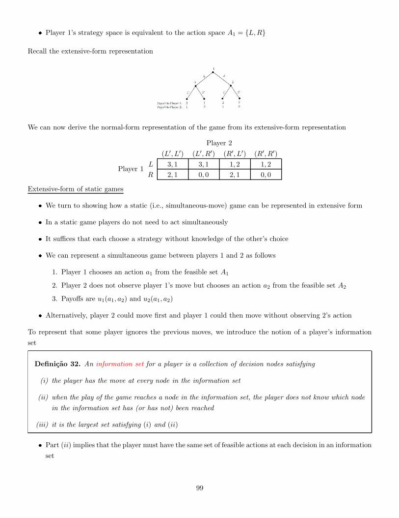
� Player 1’s strategy space is equivalent to the action space A1 = {L,R}
Recall the extensive-form representation
We can now derive the normal-form representation of the game from its extensive-form representation
Player 1
Player 2
(L′, L′) (L′, R′) (R′, L′) (R′, R′)
L 3, 1 3, 1 1, 2 1, 2
R 2, 1 0, 0 2, 1 0, 0
Extensive-form of static games
� We turn to showing how a static (i.e., simultaneous-move) game can be represented in extensive form
� In a static game players do not need to act simultaneously
� It suffices that each choose a strategy without knowledge of the other’s choice
� We can represent a simultaneous game between players 1 and 2 as follows
1. Player 1 chooses an action a1 from the feasible set A1
2. Player 2 does not observe player 1’s move but chooses an action a2 from the feasible set A2
3. Payoffs are u1(a1, a2) and u2(a1, a2)
� Alternatively, player 2 could move first and player 1 could then move without observing 2’s action
To represent that some player ignores the previous moves, we introduce the notion of a player’s information
set
Definicao 32. An information set for a player is a collection of decision nodes satisfying
(i) the player has the move at every node in the information set
(ii) when the play of the game reaches a node in the information set, the player does not know which node
in the information set has (or has not) been reached
(iii) it is the largest set satisfying (i) and (ii)
� Part (ii) implies that the player must have the same set of feasible actions at each decision in an information
set
99
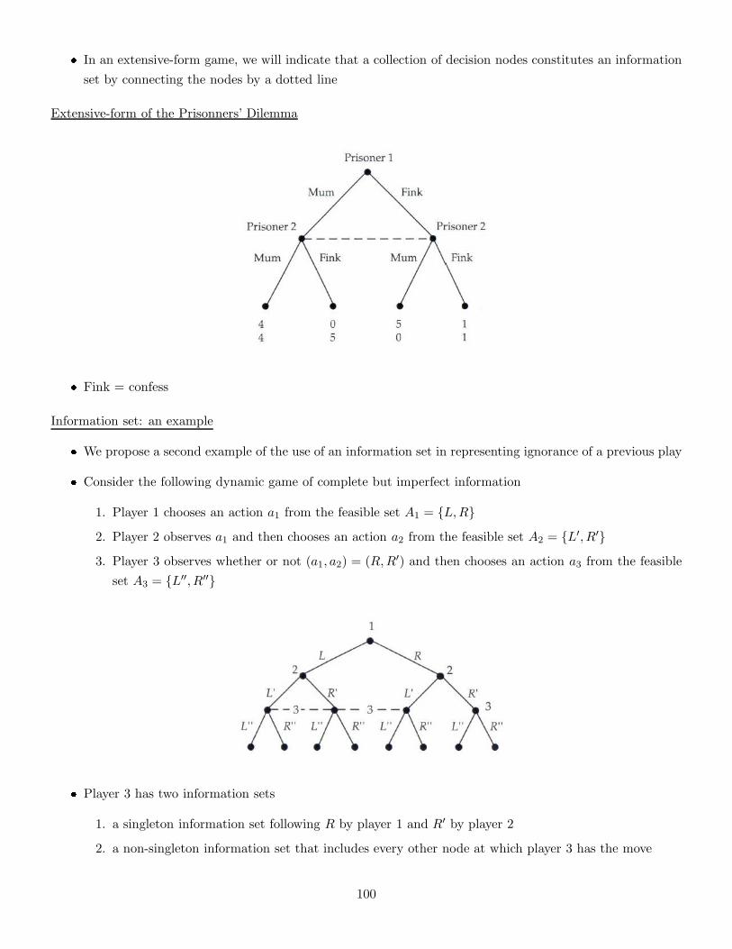
� In an extensive-form game, we will indicate that a collection of decision nodes constitutes an information
set by connecting the nodes by a dotted line
Extensive-form of the Prisonners’ Dilemma
� Fink = confess
Information set: an example
� We propose a second example of the use of an information set in representing ignorance of a previous play
� Consider the following dynamic game of complete but imperfect information
1. Player 1 chooses an action a1 from the feasible set A1 = {L,R}2. Player 2 observes a1 and then chooses an action a2 from the feasible set A2 = {L′, R′}3. Player 3 observes whether or not (a1, a2) = (R,R′) and then chooses an action a3 from the feasible
set A3 = {L′′, R′′}
� Player 3 has two information sets
1. a singleton information set following R by player 1 and R′ by player 2
2. a non-singleton information set that includes every other node at which player 3 has the move
100
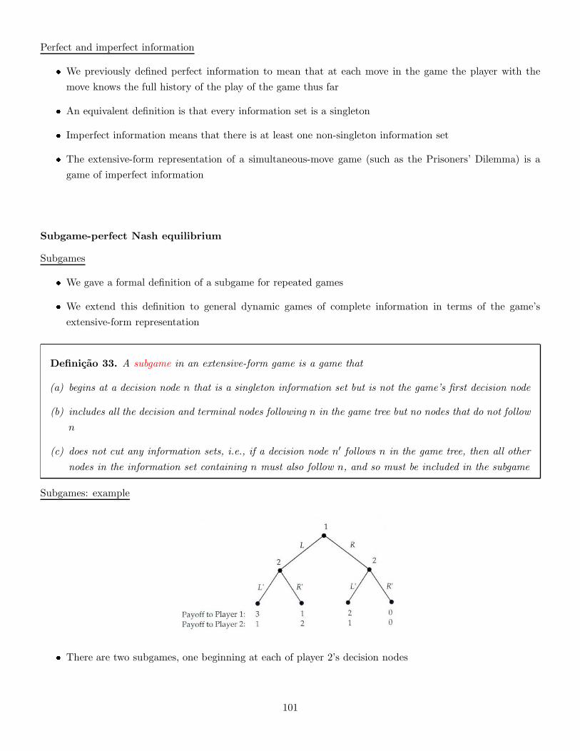
Perfect and imperfect information
� We previously defined perfect information to mean that at each move in the game the player with the
move knows the full history of the play of the game thus far
� An equivalent definition is that every information set is a singleton
� Imperfect information means that there is at least one non-singleton information set
� The extensive-form representation of a simultaneous-move game (such as the Prisoners’ Dilemma) is a
game of imperfect information
Subgame-perfect Nash equilibrium
Subgames
� We gave a formal definition of a subgame for repeated games
� We extend this definition to general dynamic games of complete information in terms of the game’s
extensive-form representation
Definicao 33. A subgame in an extensive-form game is a game that
(a) begins at a decision node n that is a singleton information set but is not the game’s first decision node
(b) includes all the decision and terminal nodes following n in the game tree but no nodes that do not follow
n
(c) does not cut any information sets, i.e., if a decision node n′ follows n in the game tree, then all other
nodes in the information set containing n must also follow n, and so must be included in the subgame
Subgames: example
� There are two subgames, one beginning at each of player 2’s decision nodes
101

Subgames: example
� There are no subgames
Subgames: example
� There is only one subgame: it begins at player 3’s decision node following R by player 1 and R′ by player
2
� Because of part (c), a subgame does not begin at either of player 2’s decision nodes, even though both of
these nodes are singleton information sets
102
Subgame perfect Nash equilibrium
Definicao 34. A profile of strategies of a dynamic game with complete information is a subgame perfect
Nash equilibrium if it is a Nash equilibrium of the initial game and the players’ strategies restricted to every
subgame constitute a Nash equilibrium of the subgame
� We already encountered two game solutions for dynamic games: backwards induction outcome and subgame
perfect outcome
� The difference is that a SPNE is a collection of strategies and a strategy is a complete plan of actions
� Whereas an outcome describes what will happen only in the contingencies that are expected to arise, not
in every contingency that might arise
Equilibrium vs outcome
Consider the standard two-stage game of complete and perfect information defined as follows
1. Player 1 chooses an action a1 from a feasible set A1
2. Player 2 observes a1 and then chooses an action a2 from a feasible set A2
3. Payoffs are u1(a1, a2) and u2(a1, a2)
Assume that for each a1 in A1, player 2’s optimization problem
argmax{u2(a1, a2) : a2 ∈ A2}
has a unique solution, denoted by R2(a1)
� Player 1’s problem at the first stage amounts to
argmax{u1(a1, R2(a1)) : a1 ∈ A1}
� Assume that the previous optimization problem for player 1 also has a unique solution, denoted by a∗1
� The pair of actions (a∗1, R2(a∗1)) is the backwards induction outcome of this game
� To define a SPNE we need to construct strategies
� For player 1 a strategy coincides with an action since there is only one contingency in which player 1 can
be called upon to act – the beginning of the game
� A strategy for player 2 is a function a1 7→ f2(a1) from A1 to A2
– R2(a∗1) is an action but not a strategy
– the best response function R2 is a possible strategy for player 2
� In this game, the subgames begin with player 2’s move in the second stage
� There is one subgame for each player 1’s feasible action a1
103
Observacao 25. The profile of strategies f∗ ≡ (a∗1, R2) is a SPNE
� We have to show that f∗ = (a∗1, R2) is a NE and that the restriction to each subgame is also a NE
� Subgames are simply single-person decision problems
– Being a NE reduces to requiring that player 2’s action be optimal in every subgame
– This is exactly the problem that the best-response function R2 solves
� Now we have to prove that f∗ is a Nash equilibrium
� Recall that a∗1 satisfies
u1(a∗1, R2(a
∗1)) ≥ u1(a1, R2(a1)) ∀a1 ∈ A1
implying that a1 is a best response to R2
� R2 is a best response to a1 since
u2(a∗1, R2(a
∗1)) ≥ u2(a
∗1, f2(a
∗1))
for every strategy f2 : A1 7→ A2
Consider the standard two-stage game of complete but imperfect information defined as follows:
� Players i1 and i2 simultaneously choose actions ai1 and ai2 from feasible sets Ai1 and Ai2 , respectively
� Players i3 and i4 observe the outcome of the first stage, (ai1 , ai2), and then simultaneously choose actions
ai3 and ai4 from feasible sets Ai3 and Ai4 , respectively
� Payoffs are ui(ai1 , ..., ai4)
� We will assume that for each feasible outcome (ai1 , ai2) of the first game, the second-stage game that
remains between players i3 and i4 has a unique NE denoted by
(ai3(ai1 , ai2), ai4(ai1 , ai2))
� Assume that (ai1 , ai2) is the unique NE of the first-stage interaction between i1 and i2 defined by the
following simultaneous-move game
1. Players i1 and i2 simultaneously choose actions ai1 and ai2 from feasible sets Ai1 and Ai2 , respectively
2. Payoffs are
ui(ai1 , ai2 , ai3(ai1 , ai2), ai4(ai1 , ai2))
Proposicao 12. In the two-stage game of complete but imperfect information defined above, the subgame
perfect outcome is
(a∗i1 , a∗i2, ai3(a
∗i1, a∗i2), ai4(a
∗i1, a∗i2))
104
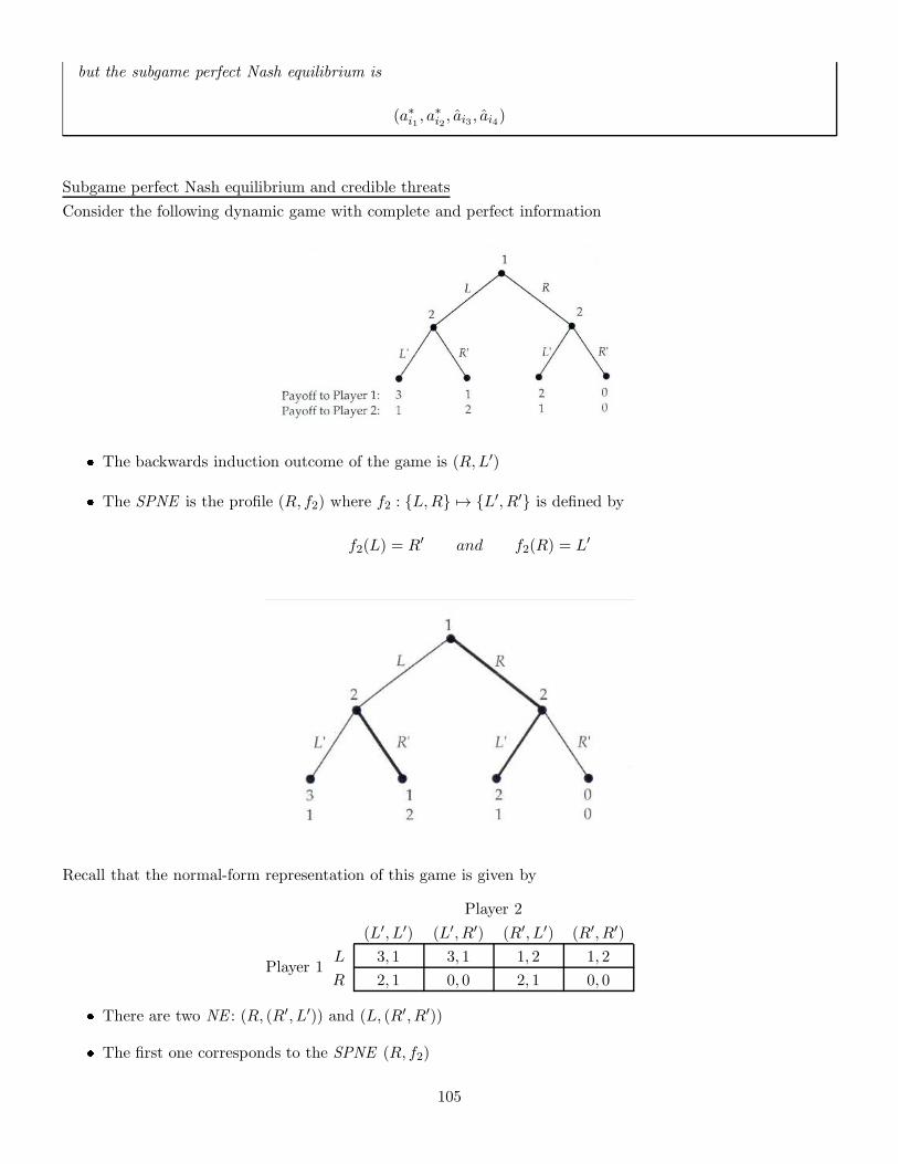
but the subgame perfect Nash equilibrium is
(a∗i1 , a∗i2, ai3 , ai4)
Subgame perfect Nash equilibrium and credible threats
Consider the following dynamic game with complete and perfect information
� The backwards induction outcome of the game is (R,L′)
� The SPNE is the profile (R, f2) where f2 : {L,R} 7→ {L′, R′} is defined by
f2(L) = R′ and f2(R) = L′
Recall that the normal-form representation of this game is given by
Player 1
Player 2
(L′, L′) (L′, R′) (R′, L′) (R′, R′)
L 3, 1 3, 1 1, 2 1, 2
R 2, 1 0, 0 2, 1 0, 0
� There are two NE : (R, (R′, L′)) and (L, (R′, R′))
� The first one corresponds to the SPNE (R, f2)
105
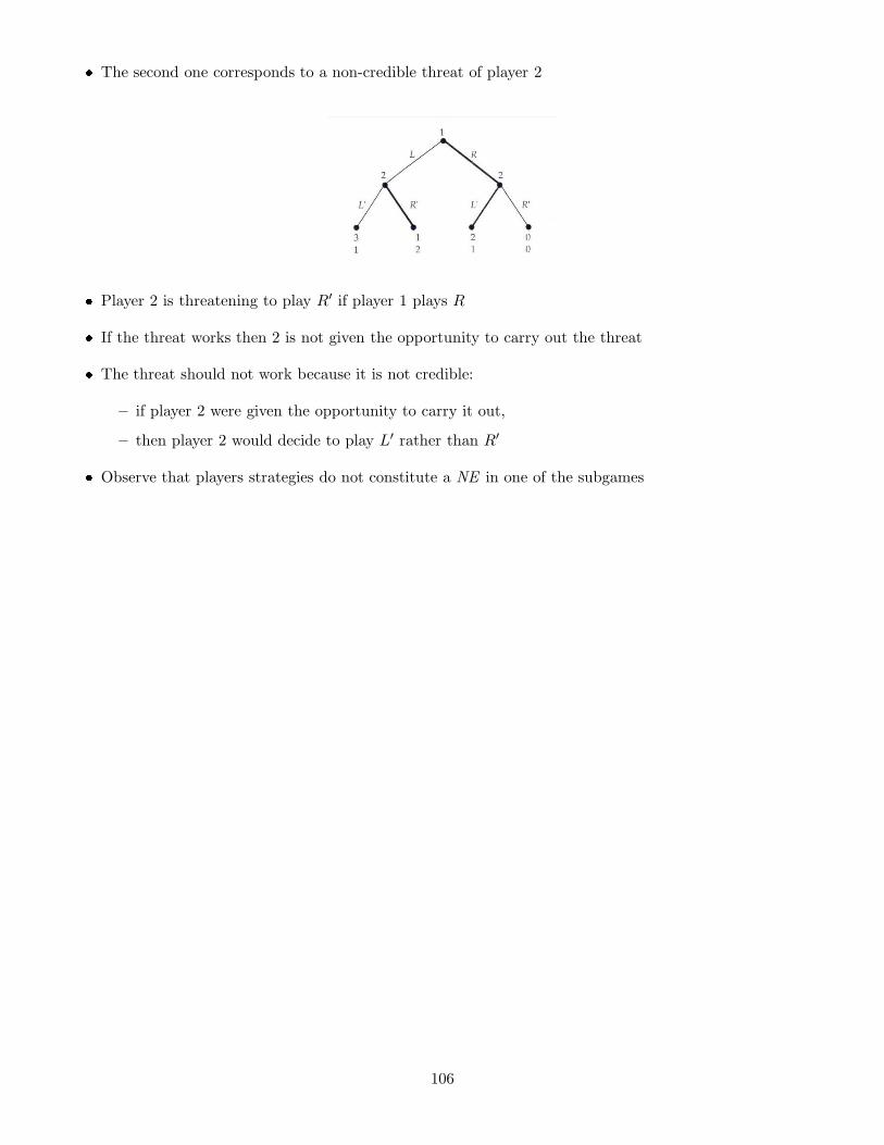
� The second one corresponds to a non-credible threat of player 2
� Player 2 is threatening to play R′ if player 1 plays R
� If the threat works then 2 is not given the opportunity to carry out the threat
� The threat should not work because it is not credible:
– if player 2 were given the opportunity to carry it out,
– then player 2 would decide to play L′ rather than R′
� Observe that players strategies do not constitute a NE in one of the subgames
106
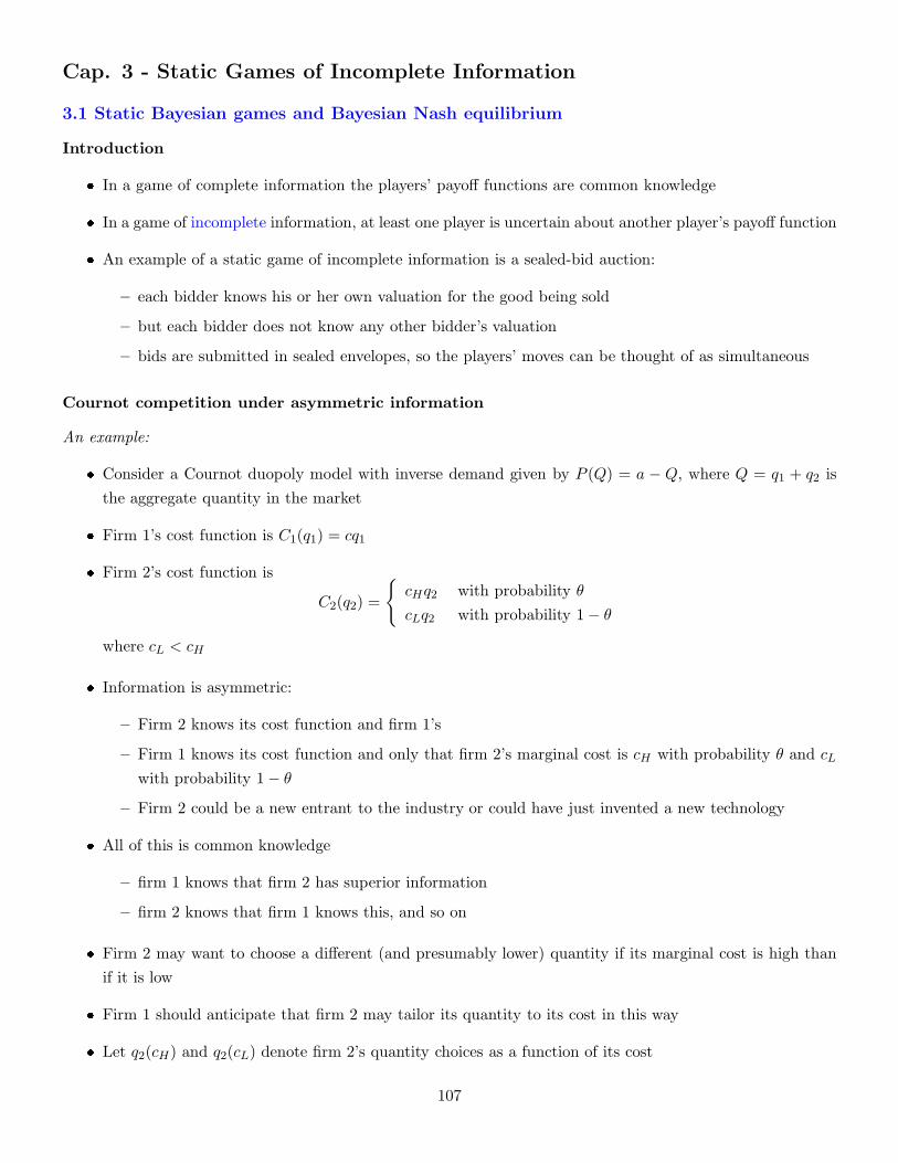
Cap. 3 - Static Games of Incomplete Information
3.1 Static Bayesian games and Bayesian Nash equilibrium
Introduction
� In a game of complete information the players’ payoff functions are common knowledge
� In a game of incomplete information, at least one player is uncertain about another player’s payoff function
� An example of a static game of incomplete information is a sealed-bid auction:
– each bidder knows his or her own valuation for the good being sold
– but each bidder does not know any other bidder’s valuation
– bids are submitted in sealed envelopes, so the players’ moves can be thought of as simultaneous
Cournot competition under asymmetric information
An example:
� Consider a Cournot duopoly model with inverse demand given by P (Q) = a − Q, where Q = q1 + q2 is
the aggregate quantity in the market
� Firm 1’s cost function is C1(q1) = cq1
� Firm 2’s cost function is
C2(q2) =
{
cHq2 with probability θ
cLq2 with probability 1− θ
where cL < cH
� Information is asymmetric:
– Firm 2 knows its cost function and firm 1’s
– Firm 1 knows its cost function and only that firm 2’s marginal cost is cH with probability θ and cL
with probability 1− θ
– Firm 2 could be a new entrant to the industry or could have just invented a new technology
� All of this is common knowledge
– firm 1 knows that firm 2 has superior information
– firm 2 knows that firm 1 knows this, and so on
� Firm 2 may want to choose a different (and presumably lower) quantity if its marginal cost is high than
if it is low
� Firm 1 should anticipate that firm 2 may tailor its quantity to its cost in this way
� Let q2(cH) and q2(cL) denote firm 2’s quantity choices as a function of its cost
107
� Let q1 denote firm 1’s single quantity choice
� If firm 2’s cost is high, it will choose q2(cH) to solve
argmax{[(a − q1 − q2)− cH ]q2 : q2 ≥ 0}
� If firm 2’s cost is low, it will choose q2(cL) to solve
argmax{[(a− q1 − q2)− cL]q2 : q2 ≥ 0}
� Firm 1 knows that firm 2’s cost is high with probability θ and should anticipate that firm 2’s quantity
choice will be q2(cH) or q2(cL), depending on firm 2’s cost
� Firm 1 chooses q1 to solve
argmax{f1(q1, q∗2) : q1 ≥ 0}
where
f1(q1, q∗2) ≡ θ[(a− q1 − q∗2(cH))− c]q1 + (1− θ)[(a− q1 − q∗2(cL))− c]q1
so as to maximize expected profits
� The first order conditions are
q∗2(cH) =a− q∗1 − cH
2
q∗2(cL) =a− q∗1 − cL
2
and
q∗1 =θ[a− q∗2(cH)− c] + (1− θ)[(a− q∗2(cL)− c]
2
� We assume that parameters are such that these FOCs characterize the solutions to the optimization
problems
The solutions to the three FOCs are
q∗2(cH) =a− 2cH + c
3+
1− θ
6(cH − cL)
q∗2(cL) =a− 2cL + c
3− θ
6(cH − cL)
and
q∗1 =a− 2c+ θcH + (1− θ)cL
3
� Consider the Cournot equilibrium under complete information with costs c1 and c2
� Under conditions on c1 and c2, firm i produces at equilibrium the quantity
qi =a− 2ci + cj
3
108
� In the incomplete information case, q∗2(cH) is greater than (a − 2cH + c)/3 and q∗2(cL) is less than (a −2cL + c)/3
� This occurs because firm 2 not only tailors its quantity to its costs
� But also responds to the fact that firm 1 cannot do so
Normal-form representation of static Bayesian games
� Recall that the normal-form representation of a game of complete information is G = (Si, ui)i∈I
– Si is player i’s strategy space
– ui(si, s−i) is player i’s payoff when he chooses the strategy si and the others choose s−i
� In a simultaneous-move game of complete information a strategy for a player is simply an action
� We can write G = (Ai, ui)i∈I where Ai is player i’s action space and ui(ai, a−i) is player i’s payoff
� The timing of a static game of complete information is as follows
1. the players simultaneously choose actions
2. payoffs are received
� We develop the normal-form representation of a simultaneous-move game of incomplete information, also
called static Bayesian game
� We should represent the idea that each player knows his or her payoff function but may be uncertain
about the other players’ payoff functions
� Let player i’s possible payoff functions be represented by ui(ai, a−i; ti) where ti is called player i’s type
� The type ti belongs to a set of possible types Ti also called type space
� Each ti corresponds to a different payoff function that player i might have
� For example, suppose that player i has two possible payoff functions
� We would say that player i has two types ti1 and ti2
� Player i’s type space is Ti = {ti1 , ti2} and player i’s two payoff functions are ui(a; ti1) and ui(a; ti2)
� We can also represent the possibility that the player might have different sets of feasible actions
– Suppose for example that player i’s set of feasible actions is {a, b} with probability q and {a, b, c}with probability 1− q
– We can say that i has two types: ti1 and ti2 where the probability of ti1 is q
109
– We can define i’s feasible set of actions to be {a, b, c} for both types but define the payoff from taking
action c to be −∞ for type ti1
Another example
� Consider the Cournot game previously presented
� The firms’ actions are their quantity choices, q1 and q2
� Firm 2 has two possible cost functions and thus two possible profit or payoff functions
π2(q1, q2; cL) = [(a− q1 − q2)− cL]q2
and
π2(q1, q2; cH) = [(a− q1 − q2)− cH ]q2
� Firm 1 has only one possible payoff function
π1(q1, q2; c) = [(a− q1 − q2)− c]q1
� We say that firm 2’s type space is T2 = {cL, cH} and that firm 1’s type space if T1 = {c}
� Saying that player i knows his or her own payoff function is equivalent to saying that player i knows his
or her type
� Saying that player i may be uncertain about the other players’ payoff functions is equivalent to saying
that player i may be uncertain about the types of the other players, denoted by
t−i = (t1, · · · , ti−1, ti+1, · · · , tn)
� We use T−i to denote the set of all possible values of t−i , i.e.,
T−i ≡∏
j 6=i
Tj = T1 × · · · × Ti−1 × Ti+1 × · · · × Tn
� We use the probability distribution π(t−i|ti) to denote player i’s belief about the other players’ types, t−i,
given player i’s knowledge of his or her own type, ti
� In many applications, the players’ types are independent, in which case π(t−i|ti) does not depend on ti,
so we can write player i’s beliefs as π(t−i)
� Imagine two firms racing to develop a new technology
� Each firm’s chance of success depends in part on how difficult the technology is to develop, which is not
known
110
� Each firm knows only whether it has succeeded and not whether the other has
� If firm 1 has succeeded, then it is more likely that the technology is easy to develop and so also more
likely that firm 2 has succeeded
� Firm 1’s belief about firm 2’s type depends on firm 1’s knowledge of its own type
Definicao 35. The normal-form representation of a static Bayesian game is
G = (Ai, Ti, pi, ui)i∈I
where
� Ai is player i’s action space
� Ti is player i’s type space
� pi ∈ Prob(T ) is player i’s beliefs about T = Ti × T−i
� ui : Ai ×A−i × Ti 7→ [−∞,∞) is player i’s payoff function
ui(ai, a−i; ti)
The normal-form representation of a static Bayesian game is
G = (Ai, Ti, pi, ui)i∈I
� Player i’s type ti is privately known by player i, determines player i’s payoff function ui(ai, a−i; ti)
� Player i’s belief
pi(t−i|ti) =pi({(ti, t−i)})pi({ti} × T−i)
describes i’s uncertainty about the other players’ possible types t−i, given i’s own type ti
111
� To simplify notations,
– pi({(ti, t−i)}) is denoted by pi(ti, t−i) or pi(t)
– pi({ti} × T−i) is denoted by pi(ti)
� Therefore
pi(t−i|ti) =pi(ti, t−i)
pi(ti)
� Since player i observes his own type, we do not need to define the probability pi on the whole space T
� One may consider as a primitive of the game the conditional probabilities
(pi(·|ti))ti∈Ti∈ [Prob(T−i)]
Ti
i.e., player i’s beliefs can be represented by a function
ti 7→ pi(·|ti)
from Ti to Prob(T−i)
Following Harsanyi (1968) we will assume that the timing of a static Bayesian game is as follows
1. Nature draws a type vector t = (ti)i∈I where ti is drawn from the set of possible types Ti
2. Nature reveals ti to player i but not to any other player
3. The players simultaneously choose actions, player i choosing ai from the feasible set Ai
4. Payoffs ui(ai, a−i; ti) are received
� We can interpret a game of incomplete information as a game of imperfect information since at some move
in the game the player with the move does not know the complete history of the game thus far
� Indeed, nature reveals player i’s type to player i but not to player j in step (2)
� Player j does not know the complete history of the game when actions are chosen in step (3)
� For some games, player i’s payoff may depend not only on the actions (ai, a−i), his type ti but also on all
the other types t−i
� In that case player i’s payoff is denoted by ui(ai, a−i; ti, t−i)
� We will assume that it is common knowledge that in step (1) of the timing, nature draws a type vector
t = (ti)i∈I according to a common prior probability distribution p ∈ Prob(T )
� When nature reveals ti to player i, he can compute the belief pi(t−i|ti) using Bayes’ rule
pi(t−i|ti) = p(t−i|ti) ≡p(ti, t−i)
p(ti)=
p(ti, t−i)∑
τ−i∈T−ip(ti, τ−i)
112
� The other players can compute the various beliefs π(·|ti) that player i might hold, depending on i’s type
ti
� We will frequently assume that players’ type are independent, i.e., there exists qi ∈ Prob(Ti) such that
p(t1, · · · , tn) = q1(t1)× · · · × qn(tn)
� In this case pi(t−i|ti) does not depend on ti since
pi(t−i|ti) = q1(t1)× · · · × qi−1(ti−1)× qi+1(ti+1)× · · · × qn(tn)
� In this case the other players know i’s belief about their types
Definition of Bayesian Nash equilibrium
� In order to define an equilibrium concept for static Bayesian games, we must first define the player’s
strategies
� Recall that a player’s strategy is a complete plan of action, specifying a feasible action in every contingency
in which the player might be called on to act
� Giving the timing of a static Bayesian game, in which nature begins the game by drawing the players’
types, a (pure) strategy for player i must specify a feasible action for each of player i’s possible types
Definicao 36. A strategy for player i in the static Bayesian game G = (Ai, Ti, pi, ui)i∈I is a function
si : Ti 7→ Ai
which specifies for each type ti ∈ Ti an action si(ti) from the feasible set Ai
� In a Bayesian game the strategy spaces are constructed from the type and action spaces
� Player i’s set of possible (pure) strategies, Si, is the set of all possible functions with domain Ti and range
Ai
Si ≡ ATi
i
� In a separating strategy, each type ti chooses a different action ai
� In a pooling strategy, all types choose the same action
� It may seem unnecessary to require player i’s strategy to specify a feasible action for each player i’s
possible types
113
� Once nature has drawn a particular type and revealed it to a player, it may seem that the player need
not be concerned with the actions he should have taken had nature drawn some other type
� But player i needs to consider what the other players will do
� What they will do depends on what the other players think player i will do, for each ti in Ti (since they
do not observe ti )
� In deciding what to do once one type has been drawn, player i will have to think about what he would
have done if each other types in Ti had been drawn
� When player j has to decide what to do, he should think about what player i may do for each possible
types in Ti, since player j cannot observe player i’s type
Definicao 37. In the static game G = (Ai, Ti, pi, ui)i∈I the profile of strategies
s∗ = (s∗i )i∈I
is a (pure strategy) Bayesian Nash equilibrium (BNE) if for each player i and for each of i’s types ti in Ti,
the action s∗i (ti) solves
argmax
∑
t−i∈T−i
ui(ai, s∗−i(t−i); (ti, t−i))pi(t−i|ti) : ai ∈ Ai
where ui(ai, s∗−i(t−i); t) is given by
ui(s∗1(t1), · · · , s∗i−1(ti−1), ai, s
∗i+1(ti+1), · · · , s∗n(tn); t)
� One may also write in condensed form
s∗i (ti) ∈ argmax{Ep[ui(ai, s∗−i)|ti] : ai ∈ Ai}
� In a static BNE, no player wants to change his strategy, even if the change involves only one action by
one type
� We can show that in a finite static Bayesian game (i.e., a game in which Ai and Ti are finite sets) there
exists a BNE, perhaps in mixed strategies
Proposicao 13. Assume that (s∗i )i∈I is a Bayesian Nash equilibrium, i.e.,
∀ti, s∗i (ti) ∈ argmax{Ep[ui(ai, s∗−i)|ti] : ai ∈ Ai}
Then we have
s∗i ∈ argmax{Ep[ui(si, s∗−i)] : si ∈ Si = [Ai]
Ti}
114
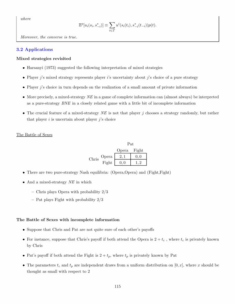
where
Ep[ui(si, s
∗−i)] ≡
∑
t∈T
ui(si(ti), s∗−i(t−i))p(t).
Moreover, the converse is true.
3.2 Applications
Mixed strategies revisited
� Harsanyi (1973) suggested the following interpretation of mixed strategies
� Player j’s mixed strategy represents player i’s uncertainty about j’s choice of a pure strategy
� Player j’s choice in turn depends on the realization of a small amount of private information
� More precisely, a mixed-strategy NE in a game of complete information can (almost always) be interpreted
as a pure-strategy BNE in a closely related game with a little bit of incomplete information
� The crucial feature of a mixed-strategy NE is not that player j chooses a strategy randomly, but rather
that player i is uncertain about player j’s choice
The Battle of Sexes
Chris
Pat
Opera Fight
Opera 2, 1 0, 0
Fight 0, 0 1, 2
� There are two pure-strategy Nash equilibria: (Opera,Opera) and (Fight,Fight)
� And a mixed-strategy NE in which
– Chris plays Opera with probability 2/3
– Pat plays Fight with probability 2/3
The Battle of Sexes with incomplete information
� Suppose that Chris and Pat are not quite sure of each other’s payoffs
� For instance, suppose that Chris’s payoff if both attend the Opera is 2 + tc , where tc is privately known
by Chris
� Pat’s payoff if both attend the Fight is 2 + tp, where tp is privately known by Pat
� The parameters tc and tp are independent draws from a uniform distribution on [0, x], where x should be
thought as small with respect to 2
115
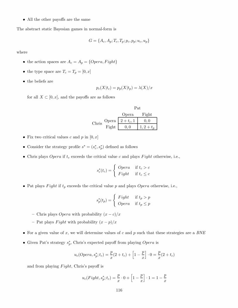
� All the other payoffs are the same
The abstract static Bayesian games in normal-form is
G = {Ac, Ap;Tc, Tp; pc, pp;uc, up}
where
� the action spaces are Ac = Ap = {Opera, F ight}
� the type space are Tc = Tp = [0, x]
� the beliefs are
pc(X|tc) = pp(X|tp) = λ(X)/x
for all X ⊂ [0, x], and the payoffs are as follows
Chris
Pat
Opera Fight
Opera 2 + tc, 1 0, 0
Fight 0, 0 1, 2 + tp
� Fix two critical values c and p in [0, x]
� Consider the strategy profile s∗ = (s∗c , s∗p) defined as follows
� Chris plays Opera if tc exceeds the critical value c and plays Fight otherwise, i.e.,
s∗c(tc) =
{
Opera if tc > c
Fight if tc ≤ c
� Pat plays Fight if tp exceeds the critical value p and plays Opera otherwise, i.e.,
s∗p(tp) =
{
Fight if tp > p
Opera if tp ≤ p
– Chris plays Opera with probability (x− c)/x
– Pat plays Fight with probability (x− p)/x
� For a given value of x, we will determine values of c and p such that these strategies are a BNE
� Given Pat’s strategy s∗p, Chris’s expected payoff from playing Opera is
uc(Opera, s∗p; tc) =p
x(2 + tc) +
[
1− p
x
]
· 0 =p
x(2 + tc)
and from playing Fight, Chris’s payoff is
uc(Fight, s∗p; tc) =p
x· 0 +
[
1− p
x
]
· 1 = 1− p
x
116
� Playing Opera is optimal (best response) if and only if
tc ≥x
p− 3 ≡ c
� Given Chris’s strategy s∗c , Pat’s expected payoff from playing Fight is
up(Fight, s∗c ; tp) =[
1− c
x
]
· 0 + c
x(2 + tp) =
c
x(2 + tp)
and from playing Opera, Pat’s payoff is
up(Opera, sc; tp) =[
1− c
x
]
· 1 + c
x· 0 = 1− c
x
� Playing Fight is optimal if and only if
tp ≥x
c− 3 ≡ p
� Solvingx
p− 3 ≡ c
andx
c− 3 ≡ p
simultaneously
� Yields p = c and p2 + 3p− x = 0
� Solving the quadratic equation then shows that both
– the probability that Chris plays Opera, namely (x− c)/x, and
– the probability that Pat plays Fight, namely (x− p)/x,
equal
1− −3 +√9 + 4x
2x
which approaches 2/3 as x approaches zero
As the incomplete information disappears (x → 0), the players’ behavior in this pure-strategy BNE of the
incomplete information game approaches the players’ behavior in the mixed-strategy NE in the original game
of complete information
An auction
� Consider the following first-price, sealed-bid auction
� There are two bidders, I = {1, 2}
117
� Bidder i has a valuation vi for the good
– If bidder i gets the good and pays the price p, then i’s payoff is vi − p
� The two players’ valuations are independently and uniformly distributed on [0, 1]
� The players simultaneously submit their non-negative bids
� The higher bidder wins the good and pays the price she bid; the other bidder gets and pays nothing
� In case of a tie, the winner is determined by a flip of a coin
� The bidders are risk-neutral and all this is common knowledge
The static Bayesian game associated to this problem is defined by
� the action space Ai = [0,∞)
� the type space Ti = [0, 1]
� Player i believes that vj is uniformly distributed on [0, 1]
∀V ∈ B([0, 1]), pi({vj ∈ V }|vi) = λ(V )
where λ is the Lebesgue measure on [0, 1]
� Abusing notations, pi(·|vi) is denoted pi(·) since it is independent of vi
� Player i’s (expected) payoff function is
ui(b1, b2; v1, v2) =
vi − bi if bi > bj
(vi − bi)/2 if bi = bj
0 if bi < bj
� A strategy for player i is a function
bi : vi 7→ bi(vi)
� A profile (b1, b2) is BNE if for each player i, for each valuation vi ∈ [0, 1], the value bi(vi) belongs to
argmax
{
(vi − bi)pi{bi > bj}+1
2(vi − bi)pi{bi = bj} : bi ≥ 0
}
� Recall that
pi{bi > bj} = λ{vj ∈ [0, 1] : bi > bj(vj)}
and
pi{bi = bj} = λ{vj ∈ [0, 1] : bi = bj(vj)}
An auction: existence of a linear equilibrium
118
� We propose to look for a linear equilibrium of the form
bi : vi 7→ ai + civi
where ci > 0
� We are not restricting the players’ strategy spaces to include only linear strategies
� We allow players to choose arbitrary strategies but ask whether there is an equilibrium that is linear
� Suppose that player j adopts the linear strategy
bj = aj + cjId
where
Id : [0, 1] → [0, 1] is defined by Id(v) = v
� For a given valuation vi, player i’s best response solves
maxbi≥0
{(vi − bi)λ{bi > aj + cjId}}
where we recall that
λ{bi > aj + cjId} = λ{vj ∈ [0, 1] : bj > aj + cjvj}
� We have used the fact that λ{bi = bj} = 0
� Observe that the best reply bi(vi) must satisfy
aj ≤ bi(vi) ≤ aj + cj
� If bi belongs to [aj , aj + cj ] then
λ{bi > aj + cjId} = λ[0, (bi − aj)/cj) =bi − aj
cj
� Player i’s best response is therefore
bi(vi) =
{
(vi + aj)/2 if vi ≥ aj
aj if vi < aj
� If 0 < aj < 1 then there are some values of vi such that vi < aj , in which case bi is not linear
� Can we find a NE where aj ≥ 1 or aj ≤ 0?
� Assume that aj ≤ 0, in this case player i’s best response is
bi(vi) =aj2
+1
2vi
119
� The function bi takes the form ai + ciId where ai = aj/2 and ci = 1/2
� This implies that ((1/2)Id, (1/2)Id) is a BNE
An auction: uniqueness
� We propose to prove that there is a unique symmetric BNE which is the linear equilibrium already derived
� A BNE is called symmetric if the players’ strategies are identical
� We propose to prove that there is a single function b such that (b, b) is a BNE
� Since players’ valuations typically will be different, their bids typically will be different, even if both use
the same strategy
� Suppose that player j adopts a strategy b and assume that b is strictly increasing and differentiable
� For a given value of vi, player i’s optimal bid solves5
maxbi≥0
(vi − bi)λ{bi > b}
If bi ∈ Im(b) then
{bi > b} =[
0, b−1(bi))
implying that
−b−1(bi(vi)) + (vi − bi(vi))[
b−1]′(bi(vi)) = 0
� In order to get a symmetric BNE we need to have bi = b
� The first-order condition is then
−b−1(b(vi)) + (vi − b(vi))[
b−1]′(b(vi)) = 0
� Since we have b−1(b(vi)) = vi and[
b−1]′(b(vi)) =
1[
b]′(vi)
� Then the function b must satisfy
vi
[
b]′(vi) + b(vi) = vi
� Observe that[
Id × b]′(vi) = vi
[
b]′(vi) + b(vi)
� This leads to[
Id× b− (1/2)Id2]′
= 0
5Observe that λ{bi = b} = 0
120
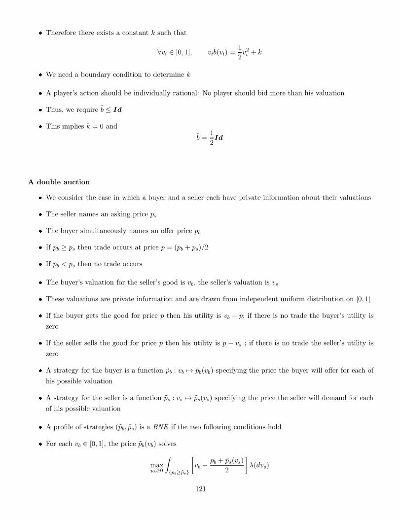
� Therefore there exists a constant k such that
∀vi ∈ [0, 1], vib(vi) =1
2v2i + k
� We need a boundary condition to determine k
� A player’s action should be individually rational: No player should bid more than his valuation
� Thus, we require b ≤ Id
� This implies k = 0 and
b =1
2Id
A double auction
� We consider the case in which a buyer and a seller each have private information about their valuations
� The seller names an asking price ps
� The buyer simultaneously names an offer price pb
� If pb ≥ ps then trade occurs at price p = (pb + ps)/2
� If pb < ps then no trade occurs
� The buyer’s valuation for the seller’s good is vb, the seller’s valuation is vs
� These valuations are private information and are drawn from independent uniform distribution on [0, 1]
� If the buyer gets the good for price p then his utility is vb − p; if there is no trade the buyer’s utility is
zero
� If the seller sells the good for price p then his utility is p − vs ; if there is no trade the seller’s utility is
zero
� A strategy for the buyer is a function pb : vb 7→ pb(vb) specifying the price the buyer will offer for each of
his possible valuation
� A strategy for the seller is a function ps : vs 7→ ps(vs) specifying the price the seller will demand for each
of his possible valuation
� A profile of strategies (pb, ps) is a BNE if the two following conditions hold
� For each vb ∈ [0, 1], the price pb(vb) solves
maxpb≥0
∫
{pb≥ps}
[
vb −pb + ps(vs)
2
]
λ(dvs)
121
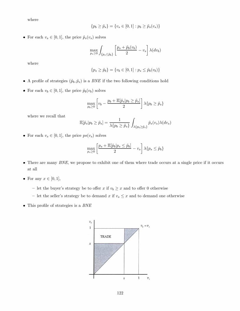
where
{pb ≥ ps} = {vs ∈ [0, 1] : pb ≥ ps(vs)}
� For each vs ∈ [0, 1], the price ps(vs) solves
maxps≥0
∫
{ps≤pb}
[ps + pb(vb)
2− vs
]
λ(dvb)
where
{ps ≥ pb} = {vb ∈ [0, 1] : ps ≤ pb(vb)}
� A profile of strategies (pb, ps) is a BNE if the two following conditions hold
� For each vb ∈ [0, 1], the price pb(vb) solves
maxpb≥0
[
vb −pb + E[ps|pb ≥ ps]
2
]
λ{pb ≥ ps}
where we recall that
E[ps|pb ≥ ps] =1
λ{pb ≥ ps}
∫
λ{pb≥ps}ps(vs)λ(dvs)
� For each vs ∈ [0, 1], the price ps(vs) solves
maxps≥0
[ps + E[pb|ps ≤ pb]
2− vs
]
λ{ps ≤ pb}
� There are many BNE, we propose to exhibit one of them where trade occurs at a single price if it occurs
at all
� For any x ∈ [0, 1],
– let the buyer’s strategy be to offer x if vb ≥ x and to offer 0 otherwise
– let the seller’s strategy be to demand x if vs ≤ x and to demand one otherwise
� This profile of strategies is a BNE
122
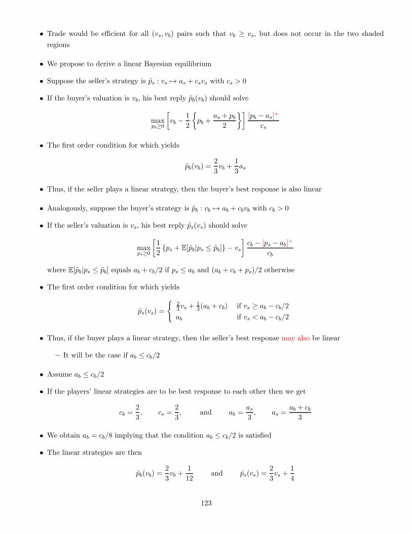
� Trade would be efficient for all (vs, vb) pairs such that vb ≥ vs, but does not occur in the two shaded
regions
� We propose to derive a linear Bayesian equilibrium
� Suppose the seller’s strategy is ps : vs 7→ as + csvs with cs > 0
� If the buyer’s valuation is vb, his best reply pb(vb) should solve
maxpb≥0
[
vb −1
2
{
pb +as + pb
2
}][pb − as]
+
cs
� The first order condition for which yields
pb(vb) =2
3vb +
1
3as
� Thus, if the seller plays a linear strategy, then the buyer’s best response is also linear
� Analogously, suppose the buyer’s strategy is pb : vb 7→ ab + cbvb with cb > 0
� If the seller’s valuation is vs, his best reply ps(vs) should solve
maxps≥0
[1
2{ps + E[pb|ps ≤ pb]} − vs
]cb − [ps − ab]
+
cb
where E[pb|ps ≤ pb] equals ab + cb/2 if ps ≤ ab and (ab + cb + ps)/2 otherwise
� The first order condition for which yields
ps(vs) =
{23vs +
13(ab + cb) if vs ≥ ab − cb/2
ab if vs < ab − cb/2
� Thus, if the buyer plays a linear strategy, then the seller’s best response may also be linear
– It will be the case if ab ≤ cb/2
� Assume ab ≤ cb/2
� If the players’ linear strategies are to be best response to each other then we get
cb =2
3, cs =
2
3, and ab =
as3, as =
ab + cb3
� We obtain ab = cb/8 implying that the condition ab ≤ cb/2 is satisfied
� The linear strategies are then
pb(vb) =2
3vb +
1
12and ps(vs) =
2
3vs +
1
4
123
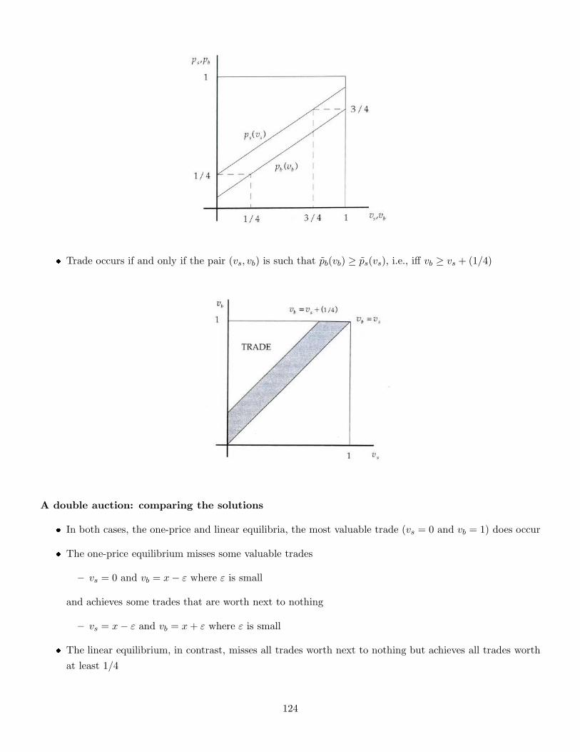
� Trade occurs if and only if the pair (vs, vb) is such that pb(vb) ≥ ps(vs), i.e., iff vb ≥ vs + (1/4)
A double auction: comparing the solutions
� In both cases, the one-price and linear equilibria, the most valuable trade (vs = 0 and vb = 1) does occur
� The one-price equilibrium misses some valuable trades
– vs = 0 and vb = x− ε where ε is small
and achieves some trades that are worth next to nothing
– vs = x− ε and vb = x+ ε where ε is small
� The linear equilibrium, in contrast, misses all trades worth next to nothing but achieves all trades worth
at least 1/4
124
� This suggests that the linear equilibrium may dominate the one-price equilibria, in terms of the expected
gains the players receive
� One may wonder if it is possible to find other BNE for which the players might do even better
� Myerson and Satterthwaite (Jet 1983) show that, for the uniform valuation distributions, the linear
equilibrium yields higher expected gains for the players than any other Bayesian Nash equilibria of the
double auction
� This implies that there is no BNE of the double auction in which trade occurs if and only if it is efficient
(i.e., if and only if vb ≥ vs)
3.3 The Revelation Principle
Desenho de Mecanismo
� E comum que um dos jogadores possa definir os termos em que um processo de interacao estrategica ira
se desenvolver
� Quando o governo decide privatizar alguma de suas empresas
– o governo e vendedor
– mas tambem e o agente que determina as regras do jogo (regras da privatizacao)
� Um empresario que decide vender sua empresa pode tambem definir os termos em que se desenvolvera a
negociacao com eventuais compradores
� O Banco Central, nos seus leiloes de tıtulos publicos, estabelece as proprias regras desses leiloes
Informacao privada e mecanismos
� O fato que alguns jogadores possuem informacao privada e essencial para que o jogador que define as
regras consiga maximizar sua recompensa
� Quando se vai vender uma empresa (ou um tıtulo do BC) em geral nao se conhece o valor que o comprador
esta disposto a pagar
� Uma regra do jogo e chamada de mecanismo
Questao 11. Como elaborar ou desenhar um mecanismo para que determinado objetivo seja alcancado?
Regras basicas do mecanismo
� O jogador que possui o poder de desenhar o mecanismo tem a liberdade de definir as regras do jogo
� No entanto, ele enfrente duas restricoes
125
1. individual rationality: o jogador responsavel pelo desenho nao pode adotar nenhuma coercao
– os jogadores envolvidos no mecanismo devem jogar de forma voluntaria
2. incentive compatibility: o jogador responsavel pelo desenho tem que ter expectativas razoaveis sobre
o comportamento dos outros jogadores
– os jogadores envolvidos no mecanismo nao irao jogar algo que nao seja um equilıbrio do mecan-
ismo consistente com seus proprios interesses
Exemplo
� Um governo decidiu vender uma empresa publica
� Apenas um comprador se qualificou em um processo previo para a aquisicao da empresa
� Existem dois tipos de comprador:
– um tipo que atribui a empresa um valor elevado a > 0
– um tipo que atribui um valor baixo b, com a > b > 0
� O governo nao sabe de que tipo e o comprador
� Mas sabe que ele pode ser de dois tipos, a ou b
� Os possıveis tipos de compradores da empresa, {a, b}, sao de conhecimento comum dos jogadores
� Seja v o valor pago pela empresa
– Se o comprador e do tipo t ∈ {a, b}, ele extraira um excedente igual a t− v
� O governo procura vender a empresa pelo maior preco possıvel
� O governo nao sabe qual e o tipo do comprador
� Ele atribui uma probabilidade p do que o comprador seja do tipo t = a
� Vamos supor que a = 30, b = 10 e p = 0.5
Exemplo: mecanismos triviais
� Existem dois mecanismos simples para o governo
1. Perguntar ao comprador qual e o tipo dele, ou de forma equivalente, e quanto ele esta disposto a
pagar pela empresa
2. Estabelecer um preco que o comprador, qualquer que seja o seu tipo, estara disposto a pagar
� No primeiro caso, o comprador sempre ira declarar que e do tipo b, que valoriza menos a empresa
– A consequencia e que a venda da empresa se dara por o valor v = b
126
� Sera o mesmo resultado do caso em que o governo estabelece um preco que seja aceitavel para qualquer
um dos dois tipos de comprador
� Ha alternativas possıveis que podem produzir melhores resultados para o governo
Exemplo: um mecanismo mais sofisticado
� O governo pode estabelecer um mecanismo em que a venda esteja assegurada se for oferecido um preco
acima de v = 17
� Se for oferecido um valor v menor (seria entao v = b) a probabilidade de a venda efetivamente se concretizar
seria de 50%
– Nesse caso o governo joga um dado de duas faces
– Essa ameaca e crıvel?
� Como v > v, o comprador tipo t = b ira preferir correr o risco de nao efetuar a compra, fazendo a oferta
mais baixa b
� Valera a pena para o comprador de alta avaliacao t = a pagar v?
� Se o comprador de alta avaliacao t = a paga v, seu excedente (payoff) e dado por a− v = 13
– Esse valor e certo (sem risco)
� Se o comprador de tipo t = a oferece o preco mais baixo
(porque oferecer mais do que b?),
seu excedente esperado (neutro ao risco) sera
1
2(a− b) +
1
20 =
a− b
2=
30 − 10
2= 10
� Assim e melhor negocio para o comprador de alta avaliacao t = a pagar o preco mais elevado estipulado
pelo governo e assegurar a aquisicao da empresa
� Esse esquema valera a pena para o governo?
� O governo vendera a empresa para um comprador de alta avaliacao com uma probabilidade p
� Para o comprador com baixa avaliacao, ha 50% de chances de o governo vender, mas tambem ha 50% de
chances de o governo cancelar a venda
� A receita esperada (neutro ao risco) do governo sera:
Prob{t = a}v + Prob{t = b}[1
2b+
1
20
]
=1
2× 17 +
1
4× 10 +
1
4× 0 = 11
� O valor esperado 11 e superior a 10 que alternativamente obteria
127
� Esse mecanismo e melhor para o governo do que o mecanismo de um so preco para ambos os tipos
Exemplo: generalizacao do mecanismo
� Sejam α > β > 0 e θ ∈ [0, 1] valores que caracterizam o seguinte mecanismo
� Para um valor pago pelo comprador igual a α, a venda e assegurada
� Para um valor igual a β, ha uma probabilidade (1− θ) de que o governo cancele a privatizacao
� O comprador de alta avaliacao (t = a) prefere comprar a empresa pagando o valor α do que correr o risco
de ofertar o valor baixo, desde que
a− α ≥ θ(a− β) i.e. , a ≥ α− θβ
1− θ
� O comprador de baixa avaliacao (t = b) prefere correr o risco de ofertar o valor baixo β do que pagar o
valor alto, se
θ(b− β) ≥ b− α i.e., b ≤ α− θβ
1− θ
� A equacao
b ≤ α− θβ
1− θ≤ a
e chamada de restricao de compatibilidade de incentivos (incentive compatibility)
� Gracas a ela, cada tipo de comprador prefere selecionar o valor a ser pago mais adequado ao seu tipo
� Estabelecendo o valor α muito alto pode estimular o comprador de alta avaliacao a incorrer o risco de
propor o valor mais baixo
� O mesmo problema ocorre se a probabilidade (1− θ) de cancelar a venda for muito baixo
� Temos que adicionar a restricao de que nenhum tipo de comprador pode ser coagido a adquirir a empresa
(i.e., participar do mecanismo)
� O lucro esperado de cada tipo de comprador tem que ser maior do que o custo de oportunidade (nao
participar do mecanismo), i.e.,
a ≥ α e b ≥ β
� Essa restricao e chamada de restricao de racionalidade individual (individual rationality)
� Dada as restricoes
b ≤ α− θβ
1− θ≤ a
� a receita esperada do governo e
pα+ (1− p)θβ
� A questao e encontrar os valores (α, β, θ) que maximizam a receita a e dadas as restricao de
128
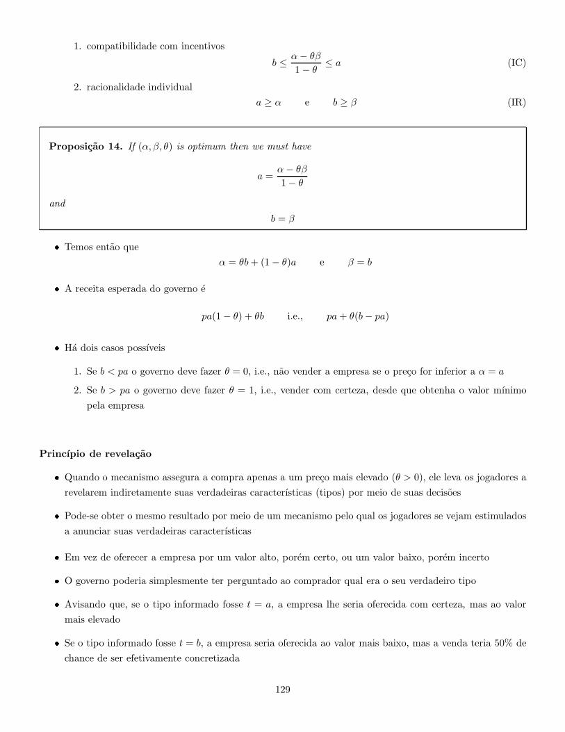
1. compatibilidade com incentivos
b ≤ α− θβ
1− θ≤ a (IC)
2. racionalidade individual
a ≥ α e b ≥ β (IR)
Proposicao 14. If (α, β, θ) is optimum then we must have
a =α− θβ
1− θ
and
b = β
� Temos entao que
α = θb+ (1− θ)a e β = b
� A receita esperada do governo e
pa(1− θ) + θb i.e., pa+ θ(b− pa)
� Ha dois casos possıveis
1. Se b < pa o governo deve fazer θ = 0, i.e., nao vender a empresa se o preco for inferior a α = a
2. Se b > pa o governo deve fazer θ = 1, i.e., vender com certeza, desde que obtenha o valor mınimo
pela empresa
Princıpio de revelacao
� Quando o mecanismo assegura a compra apenas a um preco mais elevado (θ > 0), ele leva os jogadores a
revelarem indiretamente suas verdadeiras caracterısticas (tipos) por meio de suas decisoes
� Pode-se obter o mesmo resultado por meio de um mecanismo pelo qual os jogadores se vejam estimulados
a anunciar suas verdadeiras caracterısticas
� Em vez de oferecer a empresa por um valor alto, porem certo, ou um valor baixo, porem incerto
� O governo poderia simplesmente ter perguntado ao comprador qual era o seu verdadeiro tipo
� Avisando que, se o tipo informado fosse t = a, a empresa lhe seria oferecida com certeza, mas ao valor
mais elevado
� Se o tipo informado fosse t = b, a empresa seria oferecida ao valor mais baixo, mas a venda teria 50% de
chance de ser efetivamente concretizada
129
� O resultado desse mecanismo chamado de direto seria o mesmo, apesar da forma do jogo ser diferente
� Os jogadores anunciariam seu verdadeiro tipo ao governo que em seguida atribuiria as recompensas ade-
quadas
� Eles nao teriam qualquer motivo para mentira
� Esse resultado e chamado de princıpio da revelacao
Fix
� a set of players I
� a family of types (Ti)i∈I
� a family of priors (pi)i∈I with
pi = (pi(·|ti))ti∈Tiand pi(·|ti) ∈ Prob(T−i)
Revelation principle: mechanisms
Definicao 38. A mechanism is a family
(Ai, ui)i∈I
where
� Ai is a set of available actions for player i
� ui : A× T → [−∞,∞) where
ui(ai, a−i; t)
is the payoff received by player i if he chooses ai, given that the other players choose a−i and players
type are t = (ti, t−i)
A strategy for this mechanism is a function si : Ti → Ai
Revelation principle: direct mechanisms
Definicao 39. A direct mechanism is a mechanism (Bi, vi)i∈I where
∀i ∈ I, Bi = Ti
� A strategy for a direct mechanism is a function τi : Ti → Ti
� Each agent is asked to announce his type
130
Definicao 40. A direct mechanism (vi)i∈I is said to be incentive compatible (or truth telling) if telling the
truth is a Bayesian Nash equilibrium, i.e., the strategies
(Idi)i∈I where Idi(ti) = ti
is a BNE of the Bayesian game defined by the direct mechanism.
Teorema 16 (Revelation principle). Every payoff profile (π∗i )i∈I obtained in a BNE of any mechanism
(Ai, ui)i∈I can be obtained through an incentive compatible direct mechanism, i.e., there exists a direct
mechanism (vi)i∈I which is incentive compatible and for which (π∗i )i∈I is the payoff profile of its truth
telling BNE
π∗i (ti) = E
pi [vi(ti, Id−i; (ti, ·))] =∫
T−i
vi(ti, t−i; (ti, t−i))pi(t−i|ti)
Proof. Pose
vi(τi, τ−i; t) ≡ ui(s∗i (τi), s
∗−i(τ−i); t)
where (s∗i )i∈I is the BNE of the mechanism (Ai, ui)i∈I leading to the payoff profile (πi)i∈I
131
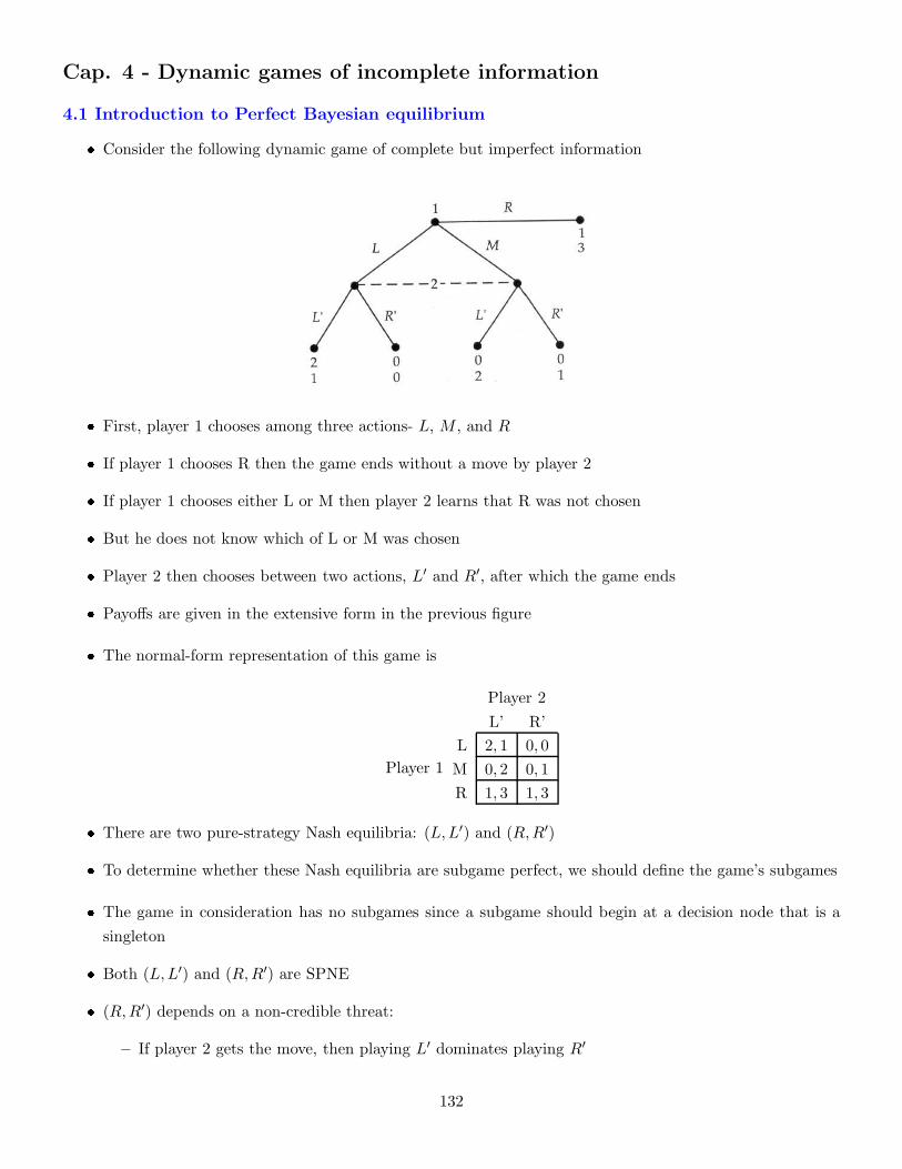
Cap. 4 - Dynamic games of incomplete information
4.1 Introduction to Perfect Bayesian equilibrium
� Consider the following dynamic game of complete but imperfect information
� First, player 1 chooses among three actions- L, M , and R
� If player 1 chooses R then the game ends without a move by player 2
� If player 1 chooses either L or M then player 2 learns that R was not chosen
� But he does not know which of L or M was chosen
� Player 2 then chooses between two actions, L′ and R′, after which the game ends
� Payoffs are given in the extensive form in the previous figure
� The normal-form representation of this game is
Player 1
Player 2
L’ R’
L 2, 1 0, 0
M 0, 2 0, 1
R 1, 3 1, 3
� There are two pure-strategy Nash equilibria: (L,L′) and (R,R′)
� To determine whether these Nash equilibria are subgame perfect, we should define the game’s subgames
� The game in consideration has no subgames since a subgame should begin at a decision node that is a
singleton
� Both (L,L′) and (R,R′) are SPNE
� (R,R′) depends on a non-credible threat:
– If player 2 gets the move, then playing L′ dominates playing R′
132
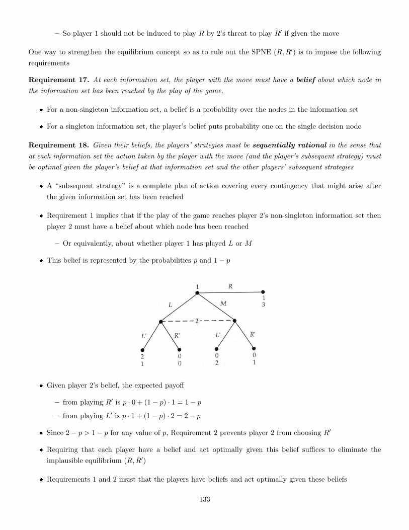
– So player 1 should not be induced to play R by 2’s threat to play R′ if given the move
One way to strengthen the equilibrium concept so as to rule out the SPNE (R,R′) is to impose the following
requirements
Requirement 17. At each information set, the player with the move must have a belief about which node in
the information set has been reached by the play of the game.
� For a non-singleton information set, a belief is a probability over the nodes in the information set
� For a singleton information set, the player’s belief puts probability one on the single decision node
Requirement 18. Given their beliefs, the players’ strategies must be sequentially rational in the sense that
at each information set the action taken by the player with the move (and the player’s subsequent strategy) must
be optimal given the player’s belief at that information set and the other players’ subsequent strategies
� A “subsequent strategy” is a complete plan of action covering every contingency that might arise after
the given information set has been reached
� Requirement 1 implies that if the play of the game reaches player 2’s non-singleton information set then
player 2 must have a belief about which node has been reached
– Or equivalently, about whether player 1 has played L or M
� This belief is represented by the probabilities p and 1− p
� Given player 2’s belief, the expected payoff
– from playing R′ is p · 0 + (1− p) · 1 = 1− p
– from playing L′ is p · 1 + (1− p) · 2 = 2− p
� Since 2− p > 1− p for any value of p, Requirement 2 prevents player 2 from choosing R′
� Requiring that each player have a belief and act optimally given this belief suffices to eliminate the
implausible equilibrium (R,R′)
� Requirements 1 and 2 insist that the players have beliefs and act optimally given these beliefs
133
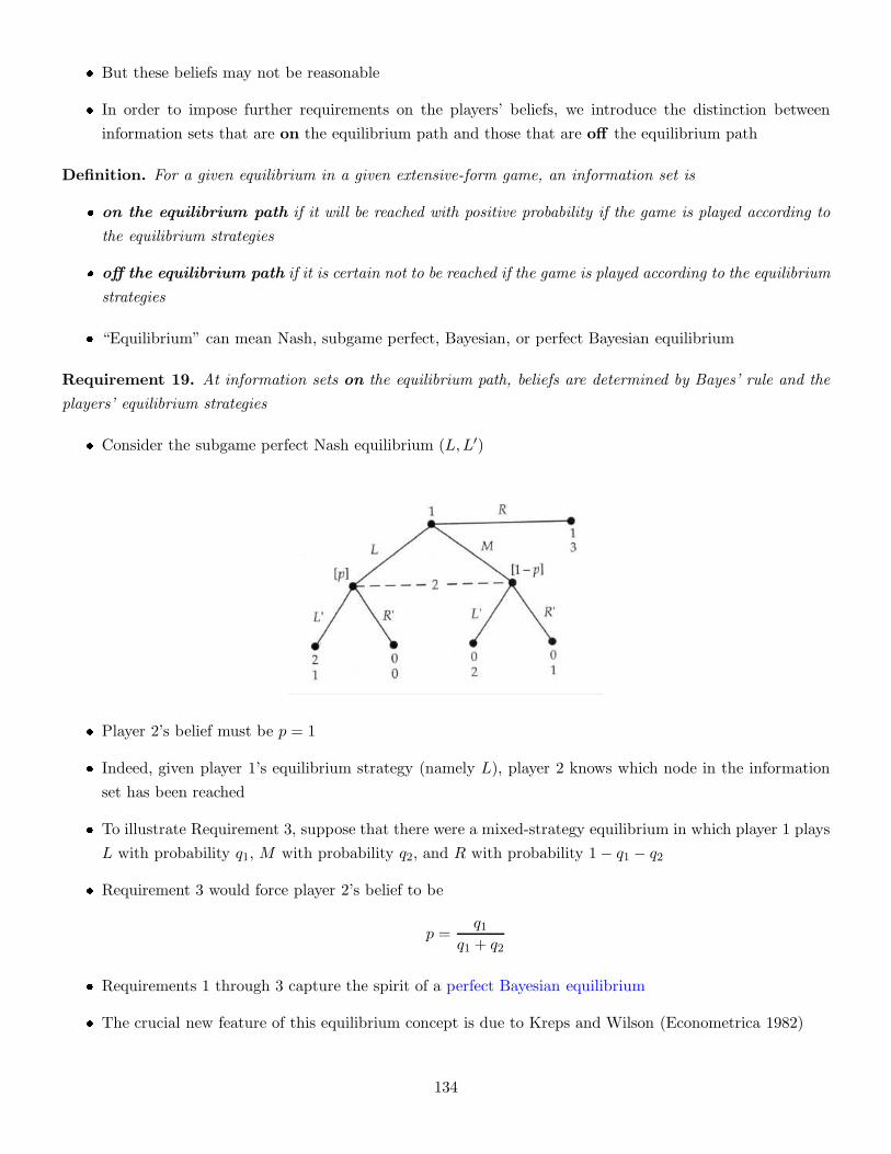
� But these beliefs may not be reasonable
� In order to impose further requirements on the players’ beliefs, we introduce the distinction between
information sets that are on the equilibrium path and those that are off the equilibrium path
Definition. For a given equilibrium in a given extensive-form game, an information set is
� on the equilibrium path if it will be reached with positive probability if the game is played according to
the equilibrium strategies
� off the equilibrium path if it is certain not to be reached if the game is played according to the equilibrium
strategies
� “Equilibrium” can mean Nash, subgame perfect, Bayesian, or perfect Bayesian equilibrium
Requirement 19. At information sets on the equilibrium path, beliefs are determined by Bayes’ rule and the
players’ equilibrium strategies
� Consider the subgame perfect Nash equilibrium (L,L′)
� Player 2’s belief must be p = 1
� Indeed, given player 1’s equilibrium strategy (namely L), player 2 knows which node in the information
set has been reached
� To illustrate Requirement 3, suppose that there were a mixed-strategy equilibrium in which player 1 plays
L with probability q1, M with probability q2, and R with probability 1− q1 − q2
� Requirement 3 would force player 2’s belief to be
p =q1
q1 + q2
� Requirements 1 through 3 capture the spirit of a perfect Bayesian equilibrium
� The crucial new feature of this equilibrium concept is due to Kreps and Wilson (Econometrica 1982)
134
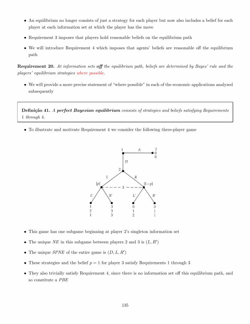
� An equilibrium no longer consists of just a strategy for each player but now also includes a belief for each
player at each information set at which the player has the move
� Requirement 3 imposes that players hold reasonable beliefs on the equilibrium path
� We will introduce Requirement 4 which imposes that agents’ beliefs are reasonable off the equilibrium
path
Requirement 20. At information sets off the equilibrium path, beliefs are determined by Bayes’ rule and the
players’ equilibrium strategies where possible.
� We will provide a more precise statement of “where possible” in each of the economic applications analyzed
subsequently
Definicao 41. A perfect Bayesian equilibrium consists of strategies and beliefs satisfying Requirements
1 through 4.
� To illustrate and motivate Requirement 4 we consider the following three-player game
� This game has one subgame beginning at player 2’s singleton information set
� The unique NE in this subgame between players 2 and 3 is (L,R′)
� The unique SPNE of the entire game is (D,L,R′)
� These strategies and the belief p = 1 for player 3 satisfy Requirements 1 through 3
� They also trivially satisfy Requirement 4, since there is no information set off this equilibrium path, and
so constitute a PBE
135
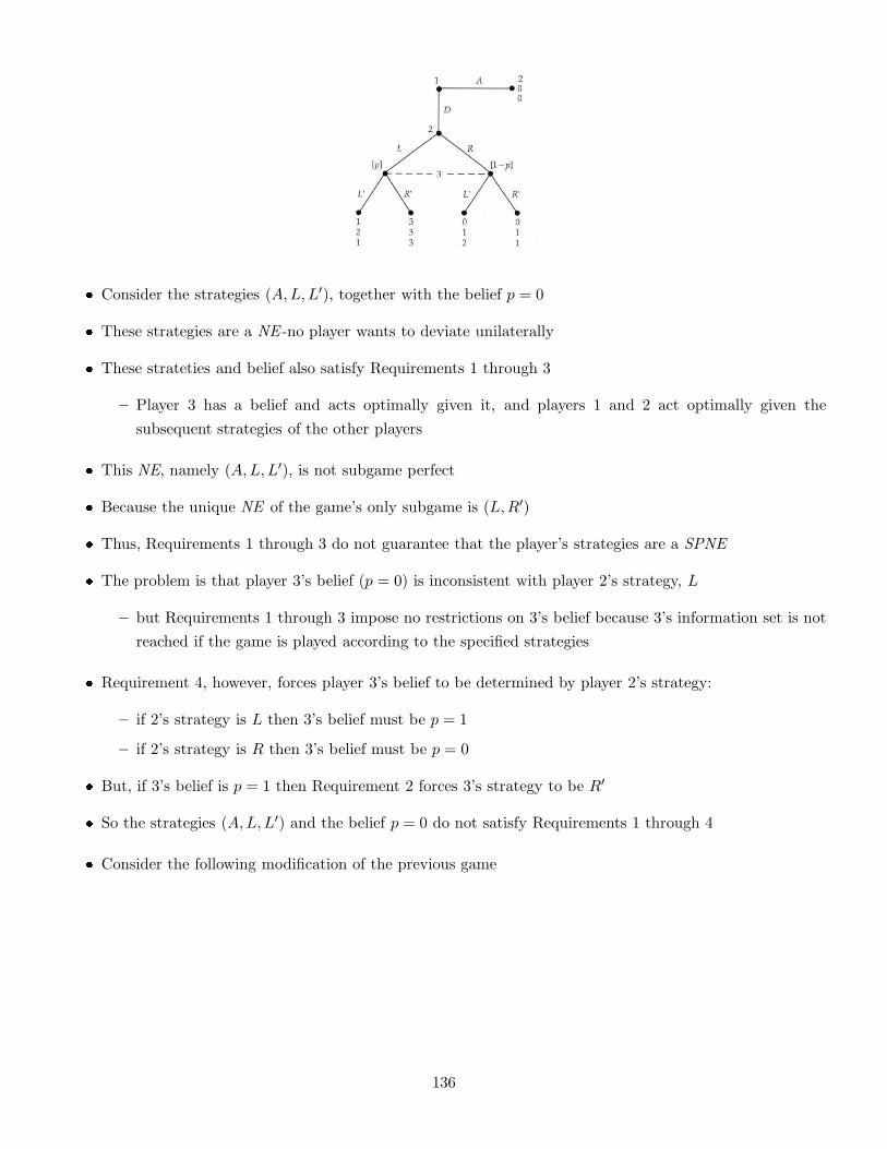
� Consider the strategies (A,L,L′), together with the belief p = 0
� These strategies are a NE -no player wants to deviate unilaterally
� These strateties and belief also satisfy Requirements 1 through 3
– Player 3 has a belief and acts optimally given it, and players 1 and 2 act optimally given the
subsequent strategies of the other players
� This NE, namely (A,L,L′), is not subgame perfect
� Because the unique NE of the game’s only subgame is (L,R′)
� Thus, Requirements 1 through 3 do not guarantee that the player’s strategies are a SPNE
� The problem is that player 3’s belief (p = 0) is inconsistent with player 2’s strategy, L
– but Requirements 1 through 3 impose no restrictions on 3’s belief because 3’s information set is not
reached if the game is played according to the specified strategies
� Requirement 4, however, forces player 3’s belief to be determined by player 2’s strategy:
– if 2’s strategy is L then 3’s belief must be p = 1
– if 2’s strategy is R then 3’s belief must be p = 0
� But, if 3’s belief is p = 1 then Requirement 2 forces 3’s strategy to be R′
� So the strategies (A,L,L′) and the belief p = 0 do not satisfy Requirements 1 through 4
� Consider the following modification of the previous game
136
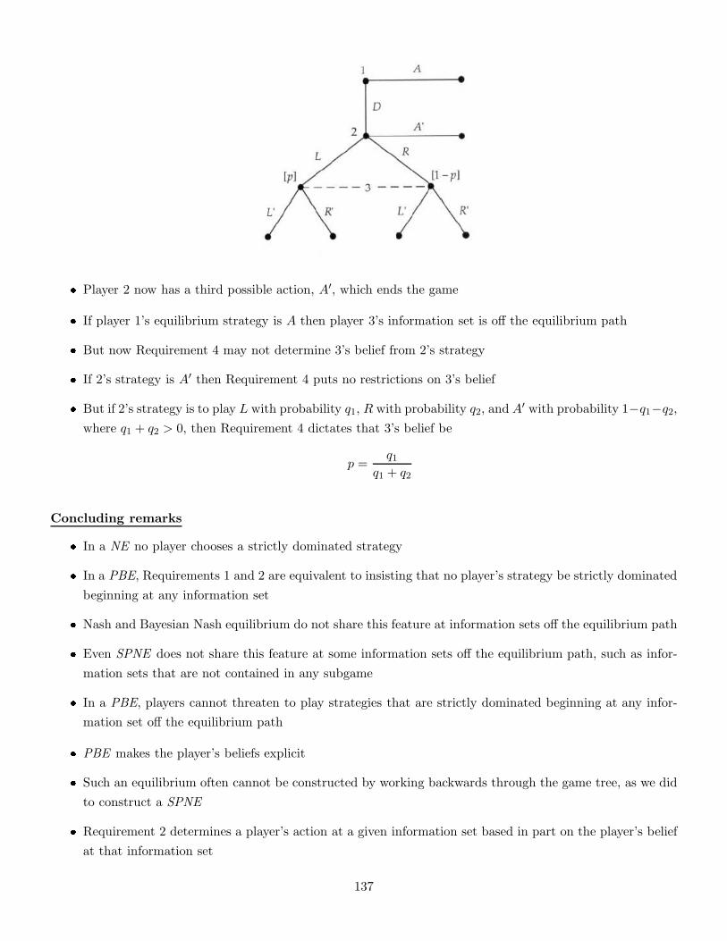
� Player 2 now has a third possible action, A′, which ends the game
� If player 1’s equilibrium strategy is A then player 3’s information set is off the equilibrium path
� But now Requirement 4 may not determine 3’s belief from 2’s strategy
� If 2’s strategy is A′ then Requirement 4 puts no restrictions on 3’s belief
� But if 2’s strategy is to play L with probability q1, R with probability q2, and A′ with probability 1−q1−q2,
where q1 + q2 > 0, then Requirement 4 dictates that 3’s belief be
p =q1
q1 + q2
Concluding remarks
� In a NE no player chooses a strictly dominated strategy
� In a PBE, Requirements 1 and 2 are equivalent to insisting that no player’s strategy be strictly dominated
beginning at any information set
� Nash and Bayesian Nash equilibrium do not share this feature at information sets off the equilibrium path
� Even SPNE does not share this feature at some information sets off the equilibrium path, such as infor-
mation sets that are not contained in any subgame
� In a PBE, players cannot threaten to play strategies that are strictly dominated beginning at any infor-
mation set off the equilibrium path
� PBE makes the player’s beliefs explicit
� Such an equilibrium often cannot be constructed by working backwards through the game tree, as we did
to construct a SPNE
� Requirement 2 determines a player’s action at a given information set based in part on the player’s belief
at that information set
137
� either Requirement 3 or 4 applies at this information set, then it determines the player’s belief from the
players’ action higher up the game tree
� But Requirement 2 determines these actions higher up the game tree based in part on the players’ subse-
quent strategies, including the action at the original information set
� This circularity implies that a single pass working backwards through the tree will not suffice to compute
a PBE
4.2 Signaling Games
Perfect Bayesian equilibrium in signaling games
A signaling game is a dynamic game of incomplete information involving two players:
� A Sender (S)
� A Receiver (R)
The timing of the game is
1. Nature draws a type ti for the Sender from a finite set of feasible types T = {t1, · · · , tI} according to a
probability distribution p ∈ Prob(T ) with full support, i.e., p(ti) > 0 for every ti
2. The Sender observes ti and then chooses a message mj from a finite set of feasible messages M =
{m1, · · · ,mJ}
3. The Receiver observes mj but not ti and then chooses an action ak from a finite set of actions A =
{a1, · · · , aK}
4. Payoffs are given by US(ti,mj, ak) and UR(ti,mj , ak)
� In many applications, the sets T , M and A are intervals on the real line, rather than finite sets
� One may allow the set of feasible messages to depend on the type Nature draws
� One may allow the set of feasible actions to depend on the message the Senders chooses
Job-market signaling
� In Spence’s (QJE 1973) model of job-market signaling
– the Sender is the worker
– the Receiver is the market of prospective employers
– the type is the worker’s productive ability
– the message is the worker’s education choice
– the action is the wage paid by the market
138
Corporate investment and capital structure
� In Myers and Majluf’s (JFE 1984) model of corporate investment and capital structure
– the Sender is a firm needing capital to finance a new project
– the Receiver is a potential investor
– the type is the profitability of the firm’s existing assets
– the message is the firm’s offer of an equity stake in return for financing
– the action is the investor’s decision about whether to invest
Monetary policy
� A signaling game may be embedded within a richer game
– there could be an action by the Receiver before the Sender chooses the message in step 2
– there could be an action by the Sender after (or while) the Receiver chooses the action in step 3
� Consider the following game:
In Vicker’s (1986) model of monetary policy
� the Federal Reserve has private information about its willingness to accept inflation in order to increase
employment
� the Sender is the Federal Reserve
� the Receiver is the market of employers
� the type is the Fed’s willingness to accept inflation in order to increase employment
� the message is the Fed’s choice of first-period inflation
� the action is the employers’ expectation of second-period inflation
� the employers’ expectation of first-period inflation precedes the signaling game
� the Fed’s choice of second-period inflation follows it
PBE definition in signaling games
� We consider an extensive form representation of a simple case: T = {t1, t2}, M = {m1,m2}, A = {a1, a2}and Prob{t1} = p
139
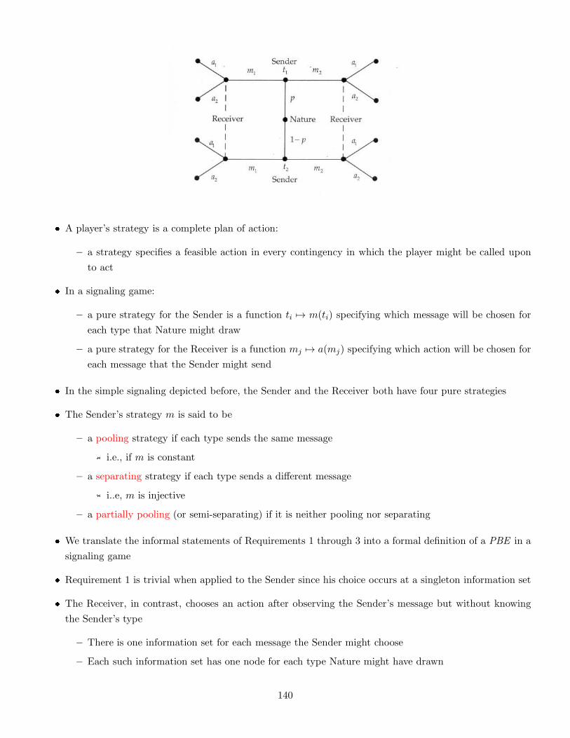
� A player’s strategy is a complete plan of action:
– a strategy specifies a feasible action in every contingency in which the player might be called upon
to act
� In a signaling game:
– a pure strategy for the Sender is a function ti 7→ m(ti) specifying which message will be chosen for
each type that Nature might draw
– a pure strategy for the Receiver is a function mj 7→ a(mj) specifying which action will be chosen for
each message that the Sender might send
� In the simple signaling depicted before, the Sender and the Receiver both have four pure strategies
� The Sender’s strategy m is said to be
– a pooling strategy if each type sends the same message
* i.e., if m is constant
– a separating strategy if each type sends a different message
* i..e, m is injective
– a partially pooling (or semi-separating) if it is neither pooling nor separating
� We translate the informal statements of Requirements 1 through 3 into a formal definition of a PBE in a
signaling game
� Requirement 1 is trivial when applied to the Sender since his choice occurs at a singleton information set
� The Receiver, in contrast, chooses an action after observing the Sender’s message but without knowing
the Sender’s type
– There is one information set for each message the Sender might choose
– Each such information set has one node for each type Nature might have drawn
140
Requirement 21 (1). After observing any message mj from M , the Receiver must have a belief about which
types could have sent mj
� Denote this belief by the probability distribution µ(·|mj) ∈ Prob(T )
Requirement 22 (2R). For each mj in M , the Receiver’s action a∗(mj) must maximize the Receiver’s expected
utility, given the belief µ(·|mj)
� That is, a∗(mj) solves
maxa∈A
∑
t∈T
µ(t|mj)UR(t,mj, a)
� Requirement 2 also applies to the Sender, but the Sender has complete information
Requirement 23 (2S). For each ti in T , the Sender’s message m∗(ti) must maximize the Sender’s utility,
given the Receiver’s strategy a∗(mj)
– That is, m∗(ti) solves
maxm∈M
US(ti,m, a∗(m))
� Given the Sender’s strategy ti 7→ m∗(ti), let Tj denote the set of types that send the message mj
Tj ≡ {ti ∈ T : m∗(ti) = mj}
or equivalently6
Tj = [m∗]−1(mj)
– The signal ti is a member of the set Tj if m∗(ti) = mj
� Given a message mj,
– if Tj is non-empty then the information set corresponding to the message mj is on the equilibrium
path
– otherwise, mj is not sent (at equilibrium) by any type and so the corresponding information set is
off the equilibrium path
For messages on the equilibrium path, one should apply Requirement 3 to the Receiver’s strategy
Requirement 24 (3). For each mj ∈ M , if there exists ti ∈ T such that m∗(ti) = mj, then the Receiver’s
belief at the information set corresponding to mj must follow from Bayes’ rule and the Sender’s strategy:
µ(ti|mj) = p(ti|[m∗]−1(mj)) =p(ti)
∑
τi∈Tjp(τi)
6Rigorously, we should write [m∗]−1({mj}).
141
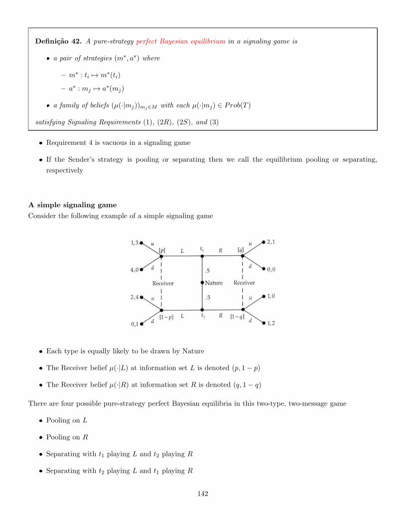
Definicao 42. A pure-strategy perfect Bayesian equilibrium in a signaling game is
� a pair of strategies (m∗, a∗) where
– m∗ : ti 7→ m∗(ti)
– a∗ : mj 7→ a∗(mj)
� a family of beliefs (µ(·|mj))mj∈M with each µ(·|mj) ∈ Prob(T )
satisfying Signaling Requirements (1), (2R), (2S), and (3)
� Requirement 4 is vacuous in a signaling game
� If the Sender’s strategy is pooling or separating then we call the equilibrium pooling or separating,
respectively
A simple signaling game
Consider the following example of a simple signaling game
� Each type is equally likely to be drawn by Nature
� The Receiver belief µ(·|L) at information set L is denoted (p, 1− p)
� The Receiver belief µ(·|R) at information set R is denoted (q, 1− q)
There are four possible pure-strategy perfect Bayesian equilibria in this two-type, two-message game
� Pooling on L
� Pooling on R
� Separating with t1 playing L and t2 playing R
� Separating with t2 playing L and t1 playing R
142
A simple signaling game: pooling on L
� Suppose there is an equilibrium (m∗, a∗, µ) in which the Sender’s strategy is
m∗(t) =
{
L if t = t1
L if t = t2
� Then the Receiver’s information set corresponding to L is on the equilibrium path
� So the Receiver’s belief (p, 1 − p) at this information set is determined by Bayes’ rule and the Sender’s
strategy
� This implies that
µ(t1|L) ≡ p =0.5
0.5 + 0.5= 0.5
� Given this belief µ, the Receiver’s best response following L is to play u
� The Sender’s type t1 earns payoff of 1 and the Sender’s type t2 earns payoff of 2
� To determine whether both “Sender types” are willing to choose L, we need to specify how the Receiver
would react to R
� If the Receiver’s response to R is u, i.e., a∗(R) = u then type t1’s payoff from playing R is 2, which exceeds
t1’s payoff of 1 from playing L
� But if the Receiver’s response to R is d, i.e., a∗(R) = d then t1 and t2 earn payoffs of 0 and 1 from playing
R, whereas they earn 1 and 2 from playing L
� To get the pooling equilibrium on L, the Receiver’s response to R must be d, i.e., a∗(R) = d
� One have to check that a∗(R) = d is an optimal action with respect to the Receiver’s belief at the
information set corresponding to R
� Observe that
Eµ(·|R)[UR(·, R, d)] = q × 0 + (1− q)× 2 = 2(1− q)
� and
Eµ(·|R)[UR(·, R, u)] = q × 1 + (1− q)× 0 = q
� Playing d is optimal for the Receiver for any q ≤ 2/3
Observacao 26. The pair of strategies (m∗, a∗) defined by
m∗(t) = L, ∀t ∈ {t1, t2}
a∗(m) =
{
u if m = L
d if m = R
143
and the beliefs m 7→ µ(·|m) defined by
µ(·|m) =
{
(0.5, 0.5) if m = L
(q, 1− q) if m = R
form a pure-strategy PBE if q ≤ 2/3.
A simple signaling game: pooling on R
� Suppose the Sender’s strategy is m∗(t) = R for any t in T
� Then q = 0.5 and the Receiver’s best response is a∗(R) = d
� Thus the contingent payoffs for the Sender are
US(t1, R, d) = 0 and US(t2, R, d) = 1
� But t1 can earn 1 by playing L, since the Receiver’s best response to L is u for any value of p
Observacao 27. There is no equilibrium in which the Sender plays m∗(t) = R for any t in T .
A simple signaling game: Separating with m∗(t1) = L
� Suppose the Sender’s strategy m∗ is defined by
m∗(t) =
{
L if t = t1
R if t = t2
� Both of the Receiver’s information sets are on the equilibrium path
� So both beliefs are determined by Bayes’ rule and the Sender’s strategy
p = 1 and q = 0
� The Receiver’s best responses to these beliefs are
a∗(m) =
{
u if m = L
d if m = R
� It remains to check whether the Sender’s strategy is optimal given the Receiver’s strategy a
� It is not:
– if type t2 deviates by playing L rather than R,
– then the Receiver’s responds with u,
144
– earning t2 a payoff of 2,
– which exceeds t2’s payoff of 1 from playing R
A simple signaling game: Separating with m∗(t1) = R
� Suppose the Sender’s strategy m is defined by
m∗(t) =
{
R if t = t1
L if t = t2
� Both of the Receiver’s information sets are on the equilibrium path
� So both beliefs are determined by Bayes’ rule and the Sender’s strategy
p = 0 and q = 1
� The Receiver’s best response to these beliefs is
a∗(m) = u, ∀m ∈ {L,R}
� Both types t1 and t2 earn payoffs of 2
� If t1 were to deviate by playing L, then the Receiver would react with u
� t1’s payoff would then be 1, so there is no incentive for t1 to deviate from playing R
� If t2 were to deviate by playing R, then the Receiver would react with u
� t2’s payoff would then be 1, so there is no incentive for t2 to deviate from playing L
Observacao 28. � The pair of strategies (m∗, a∗) defined by
m∗(t) =
{
R if t = t1
L if t = t2
a∗(m) = u, ∀m ∈ {L,R}
� and the beliefs m 7→ µ(·|m) defined by
µ(·|m) =
{
(0, 1) if m = L
(1, 0) if m = R
form a separating pure-strategy perfect Bayesian equilibrium
145
Job market signaling
� We restate Spence’s (QJE 1973) model as an extensive-form game and describe some of its perfect Bayesian
equilibria
� The timing is as follows
1. Nature determines a worker’s productive ability, η, which can be either high H or low L. The
probability that η = H is q
2. The worker learns his or her ability and then chooses a level of education, e ≥ 0
3. Two firms observe the worker’s education but not the worker’s ability, and then simultaneously make
wage offers to the worker
4. The worker accepts the higher of the two wage offers, flipping a coin in case of a tie
Payoffs
� Let w denote the wage the worker accepts
� The payoff to worker is
w − c(η, e)
where c(η, e) is the cost to a worker with ability η of obtaining education e
� The payoff to the firm that employs the worker is
y(η, e) − w
where y(η, e) is the output of a worker with ability η who has obtained education e
� The payoff to the firm that does not employ the worker is zero
Assumption on production
� We allow for the possibility that output increases not only with ability but also with education
� We assume that high-ability workers are more productive, i.e.,
∀e, y(H, e) > y(L, e)
� We assume that education does not reduce productivity, i.e.,
∀(η, e), ye(η, e) ≥ 0
where ye(η, e) is the marginal productivity of education for a worker of ability η at education e
ye(η, e) =∂y
∂e(η, e) ≥ 0
146
Interpretation of education
� We interpret differences in e as differences in the quality of a student’s performance
� Not as differences in the duration of the student’s schooling
� Thus, the game could apply to a cohort of high school graduates, or to a cohort of college graduates or
MBAs
� Under this interpretation, e measures the number and kind of courses taken and the caliber of grades and
distinctions earned during an academic program of fixed length
� Tuition costs (if they exist at all) are independent of e, so the cost function c(η, e) measures non-monetary
(or psychic) costs
� Students of lower ability find it more difficult to achieve high grades at a given school, and also more
difficult to achieve the same grades at a more competitive school
� Firm’s use of education as a signal thus reflects the fact that firms hire and pay more to the best graduates
of a given school and to the graduates of the best schools
Assumption on costs
� The crucial assumption in Spence’s model is that low-ability workers find signaling more costly than do
high-ability workers
� More precisely, we assume that the marginal cost of education is higher for low-ability than for high-ability
workers
∀e, ce(L, e) > ce(H, e)
where ce(η, e) denoted the marginal cost of education for a worker of ability η at education e
ce(η, e) =∂c
∂e(η, e)
Assumption on costs: Interpretation
� Consider a worker believing that with education e1 he would get paid wage w1
� We investigate the increase in wages that would be necessary to compensate this worker for an increase
in education from e1 to e2
� The answer depends on the worker’s ability:
– Low-ability workers find it more difficult to acquire the extra education and so require a larger
increase in wages to compensate them for it
∆w = w2 − w1 =
∫ e2
e1
∂c
∂e(η, e)de
147
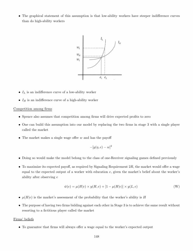
� The graphical statement of this assumption is that low-ability workers have steeper indifference curves
than do high-ability workers
� IL is an indifference curve of a low-ability worker
� IH is an indifference curve of a high-ability worker
Competition among firms
� Spence also assumes that competition among firms will drive expected profits to zero
� One can build this assumption into our model by replacing the two firms in stage 3 with a single player
called the market
� The market makes a single wage offer w and has the payoff
−[y(η, e) − w]2
� Doing so would make the model belong to the class of one-Receiver signaling games defined previously
� To maximize its expected payoff, as required by Signaling Requirement 2R, the market would offer a wage
equal to the expected output of a worker with education e, given the market’s belief about the worker’s
ability after observing e
w(e) = µ(H|e)× y(H, e) + [1− µ(H|e)] × y(L, e) (W)
� µ(H|e) is the market’s assessment of the probability that the worker’s ability is H
� The purpose of having two firms bidding against each other in Stage 3 is to achieve the same result without
resorting to a fictitious player called the market
Firms’ beliefs
� To guarantee that firms will always offer a wage equal to the worker’s expected output
148
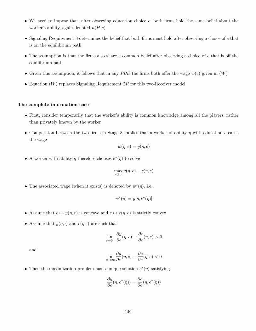
� We need to impose that, after observing education choice e, both firms hold the same belief about the
worker’s ability, again denoted µ(H|e)
� Signaling Requirement 3 determines the belief that both firms must hold after observing a choice of e that
is on the equilibrium path
� The assumption is that the firms also share a common belief after observing a choice of e that is off the
equilibrium path
� Given this assumption, it follows that in any PBE the firms both offer the wage w(e) given in (W )
� Equation (W ) replaces Signaling Requirement 2R for this two-Receiver model
The complete information case
� First, consider temporarily that the worker’s ability is common knowledge among all the players, rather
than privately known by the worker
� Competition between the two firms in Stage 3 implies that a worker of ability η with education e earns
the wage
w(η, e) = y(η, e)
� A worker with ability η therefore chooses e∗(η) to solve
maxe≥0
y(η, e) − c(η, e)
� The associated wage (when it exists) is denoted by w∗(η), i.e.,
w∗(η) = y[η, e∗(η)]
� Assume that e 7→ y(η, e) is concave and e 7→ c(η, e) is strictly convex
� Assume that y(η, ·) and c(η, ·) are such that
lime→0+
∂y
∂e(η, e) − ∂c
∂e(η, e) > 0
and
lime→∞
∂y
∂e(η, e) − ∂c
∂e(η, e) < 0
� Then the maximization problem has a unique solution e∗(η) satisfying
∂y
∂e(η, e∗(η)) =
∂c
∂e(η, e∗(η))
149
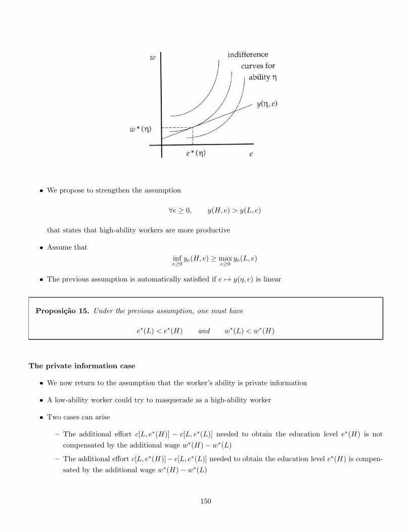
� We propose to strengthen the assumption
∀e ≥ 0, y(H, e) > y(L, e)
that states that high-ability workers are more productive
� Assume that
infe≥0
ye(H, e) ≥ maxe≥0
ye(L, e)
� The previous assumption is automatically satisfied if e 7→ y(η, e) is linear
Proposicao 15. Under the previous assumption, one must have
e∗(L) < e∗(H) and w∗(L) < w∗(H)
The private information case
� We now return to the assumption that the worker’s ability is private information
� A low-ability worker could try to masquerade as a high-ability worker
� Two cases can arise
– The additional effort c[L, e∗(H)] − c[L, e∗(L)] needed to obtain the education level e∗(H) is not
compensated by the additional wage w∗(H)− w∗(L)
– The additional effort c[L, e∗(H)]− c[L, e∗(L)] needed to obtain the education level e∗(H) is compen-
sated by the additional wage w∗(H)− w∗(L)
150
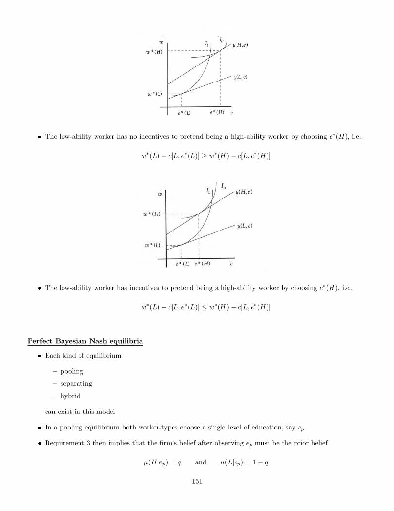
� The low-ability worker has no incentives to pretend being a high-ability worker by choosing e∗(H), i.e.,
w∗(L)− c[L, e∗(L)] ≥ w∗(H)− c[L, e∗(H)]
� The low-ability worker has incentives to pretend being a high-ability worker by choosing e∗(H), i.e.,
w∗(L)− c[L, e∗(L)] ≤ w∗(H)− c[L, e∗(H)]
Perfect Bayesian Nash equilibria
� Each kind of equilibrium
– pooling
– separating
– hybrid
can exist in this model
� In a pooling equilibrium both worker-types choose a single level of education, say ep
� Requirement 3 then implies that the firm’s belief after observing ep must be the prior belief
µ(H|ep) = q and µ(L|ep) = 1− q
151
� This in turn implies that the wage offered by the firm after observing ep must be
wp = q × y(H, ep) + (1− q)× y(L, ep)
� To complete the description of a pooling PBE, it remains
1. to specify the firm’s belief µ(·|e) for out-of-equilibrium education choices e 6= ep (Requirement 1)
2. these beliefs will then determine the firm’s strategy e 7→ w(e) through
w(e) = µ(H|e)× y(H, e) + [1− µ(H|e)] × y(L, e) (W)
(Requirement 2R)
3. to show that both worker-types’ best response to the firm’s strategy w is to choose e = ep (Require-
ment 2S)
Pooling equilibrium
� One possibility is that the firms believe that any education level other than ep implies that the worker
has low ability
∀e 6= ep, µ(H|e) = 0
� Nothing in the definition of PBE rules these beliefs out
– Requirements 1 through 2 put no restrictions on beliefs off the equilibrium path
– Requirement 4 is vacuous in a signaling game
� The refinement we will introduce in a subsequent chapter will rule out the beliefs analyzed here
� If the firm’s beliefs are
µ(H|e) ={
0 for e 6= ep
q for e = ep
� Then Equation (W) implies that the firms’ strategy is
w(e) =
{
y(L, e) for e 6= ep
wp for e = ep
where we recall that
wp = q × y(H, ep) + (1− q)× y(L, ep)
� A worker of ability η chooses e to solve
maxe≥0
w(e) − c(η, e)
152
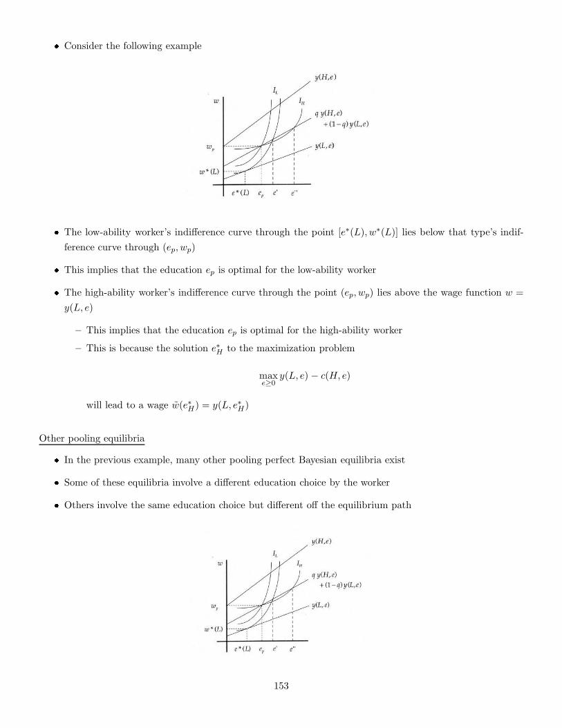
� Consider the following example
� The low-ability worker’s indifference curve through the point [e∗(L), w∗(L)] lies below that type’s indif-
ference curve through (ep, wp)
� This implies that the education ep is optimal for the low-ability worker
� The high-ability worker’s indifference curve through the point (ep, wp) lies above the wage function w =
y(L, e)
– This implies that the education ep is optimal for the high-ability worker
– This is because the solution e∗H to the maximization problem
maxe≥0
y(L, e) − c(H, e)
will lead to a wage w(e∗H) = y(L, e∗H)
Other pooling equilibria
� In the previous example, many other pooling perfect Bayesian equilibria exist
� Some of these equilibria involve a different education choice by the worker
� Others involve the same education choice but different off the equilibrium path
153
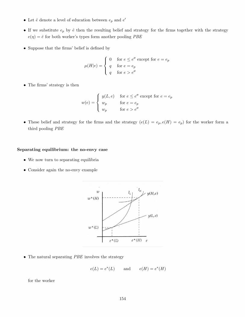
� Let e denote a level of education between ep and e′
� If we substitute ep by e then the resulting belief and strategy for the firms together with the strategy
e(η) = e for both worker’s types form another pooling PBE
� Suppose that the firms’ belief is defined by
µ(H|e) =
0 for e ≤ e′′ except for e = ep
q for e = ep
q for e > e′′
� The firms’ strategy is then
w(e) =
y(L, e) for e ≤ e′′ except for e = ep
wp for e = ep
wp for e > e′′
� These belief and strategy for the firms and the strategy (e(L) = ep, e(H) = ep) for the worker form a
third pooling PBE
Separating equilibrium: the no-envy case
� We now turn to separating equilibria
� Consider again the no-envy example
� The natural separating PBE involves the strategy
e(L) = e∗(L) and e(H) = e∗(H)
for the worker
154
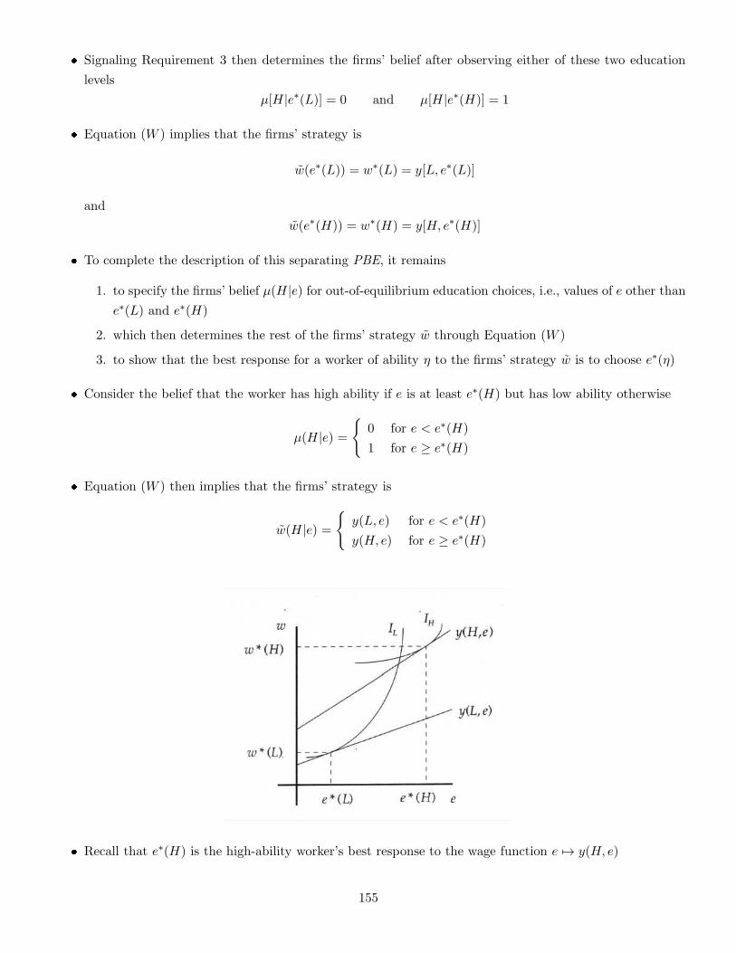
� Signaling Requirement 3 then determines the firms’ belief after observing either of these two education
levels
µ[H|e∗(L)] = 0 and µ[H|e∗(H)] = 1
� Equation (W ) implies that the firms’ strategy is
w(e∗(L)) = w∗(L) = y[L, e∗(L)]
and
w(e∗(H)) = w∗(H) = y[H, e∗(H)]
� To complete the description of this separating PBE, it remains
1. to specify the firms’ belief µ(H|e) for out-of-equilibrium education choices, i.e., values of e other than
e∗(L) and e∗(H)
2. which then determines the rest of the firms’ strategy w through Equation (W )
3. to show that the best response for a worker of ability η to the firms’ strategy w is to choose e∗(η)
� Consider the belief that the worker has high ability if e is at least e∗(H) but has low ability otherwise
µ(H|e) ={
0 for e < e∗(H)
1 for e ≥ e∗(H)
� Equation (W ) then implies that the firms’ strategy is
w(H|e) ={
y(L, e) for e < e∗(H)
y(H, e) for e ≥ e∗(H)
� Recall that e∗(H) is the high-ability worker’s best response to the wage function e 7→ y(H, e)
155
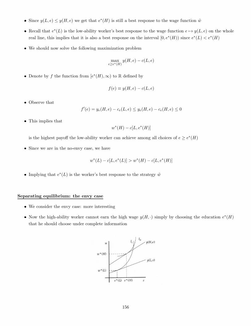
� Since y(L, e) ≤ y(H, e) we get that e∗(H) is still a best response to the wage function w
� Recall that e∗(L) is the low-ability worker’s best response to the wage function e 7→ y(L, e) on the whole
real line, this implies that it is also a best response on the interval [0, e∗(H)) since e∗(L) < e∗(H)
� We should now solve the following maximization problem
maxe≥e∗(H)
y(H, e)− c(L, e)
� Denote by f the function from [e∗(H),∞) to R defined by
f(e) ≡ y(H, e) − c(L, e)
� Observe that
f ′(e) = ye(H, e)− ce(L, e) ≤ ye(H, e) − ce(H, e) ≤ 0
� This implies that
w∗(H)− c[L, e∗(H)]
is the highest payoff the low-ability worker can achieve among all choices of e ≥ e∗(H)
� Since we are in the no-envy case, we have
w∗(L)− c[L, e∗(L)] > w∗(H)− c[L, e∗(H)]
� Implying that e∗(L) is the worker’s best response to the strategy w
Separating equilibrium: the envy case
� We consider the envy case: more interesting
� Now the high-ability worker cannot earn the high wage y(H, ·) simply by choosing the education e∗(H)
that he should choose under complete information
156
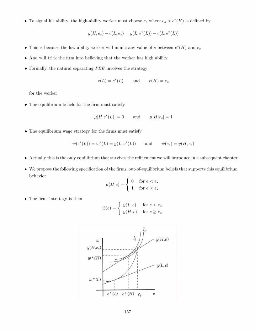
� To signal his ability, the high-ability worker must choose es where es > e∗(H) is defined by
y(H, es)− c(L, es) = y(L, e∗(L))− c(L, e∗(L))
� This is because the low-ability worker will mimic any value of e between e∗(H) and es
� And will trick the firm into believing that the worker has high ability
� Formally, the natural separating PBE involves the strategy
e(L) = e∗(L) and e(H) = es
for the worker
� The equilibrium beliefs for the firm must satisfy
µ[H|e∗(L)] = 0 and µ[H|es] = 1
� The equilibrium wage strategy for the firms must satisfy
w(e∗(L)) = w∗(L) = y(L, e∗(L)) and w(es) = y(H, es)
� Actually this is the only equilibrium that survives the refinement we will introduce in a subsequent chapter
� We propose the following specification of the firms’ out-of-equilibrium beliefs that supports this equilibrium
behavior
µ(H|e) ={
0 for e < es
1 for e ≥ es
� The firms’ strategy is then
w(e) =
{
y(L, e) for e < es
y(H, e) for e ≥ es
157
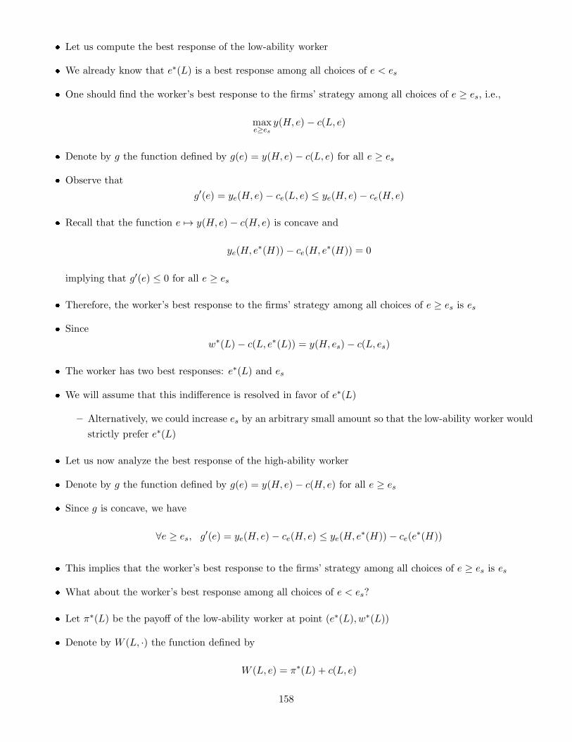
� Let us compute the best response of the low-ability worker
� We already know that e∗(L) is a best response among all choices of e < es
� One should find the worker’s best response to the firms’ strategy among all choices of e ≥ es, i.e.,
maxe≥es
y(H, e) − c(L, e)
� Denote by g the function defined by g(e) = y(H, e)− c(L, e) for all e ≥ es
� Observe that
g′(e) = ye(H, e) − ce(L, e) ≤ ye(H, e)− ce(H, e)
� Recall that the function e 7→ y(H, e)− c(H, e) is concave and
ye(H, e∗(H)) − ce(H, e∗(H)) = 0
implying that g′(e) ≤ 0 for all e ≥ es
� Therefore, the worker’s best response to the firms’ strategy among all choices of e ≥ es is es
� Since
w∗(L)− c(L, e∗(L)) = y(H, es)− c(L, es)
� The worker has two best responses: e∗(L) and es
� We will assume that this indifference is resolved in favor of e∗(L)
– Alternatively, we could increase es by an arbitrary small amount so that the low-ability worker would
strictly prefer e∗(L)
� Let us now analyze the best response of the high-ability worker
� Denote by g the function defined by g(e) = y(H, e)− c(H, e) for all e ≥ es
� Since g is concave, we have
∀e ≥ es, g′(e) = ye(H, e) − ce(H, e) ≤ ye(H, e∗(H)) − ce(e∗(H))
� This implies that the worker’s best response to the firms’ strategy among all choices of e ≥ es is es
� What about the worker’s best response among all choices of e < es?
� Let π∗(L) be the payoff of the low-ability worker at point (e∗(L), w∗(L))
� Denote by W (L, ·) the function defined by
W (L, e) = π∗(L) + c(L, e)
158
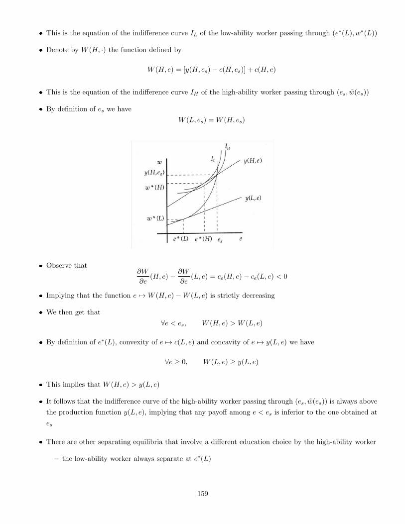
� This is the equation of the indifference curve IL of the low-ability worker passing through (e∗(L), w∗(L))
� Denote by W (H, ·) the function defined by
W (H, e) = [y(H, es)− c(H, es)] + c(H, e)
� This is the equation of the indifference curve IH of the high-ability worker passing through (es, w(es))
� By definition of es we have
W (L, es) = W (H, es)
� Observe that∂W
∂e(H, e)− ∂W
∂e(L, e) = ce(H, e)− ce(L, e) < 0
� Implying that the function e 7→ W (H, e)−W (L, e) is strictly decreasing
� We then get that
∀e < es, W (H, e) > W (L, e)
� By definition of e∗(L), convexity of e 7→ c(L, e) and concavity of e 7→ y(L, e) we have
∀e ≥ 0, W (L, e) ≥ y(L, e)
� This implies that W (H, e) > y(L, e)
� It follows that the indifference curve of the high-ability worker passing through (es, w(es)) is always above
the production function y(L, e), implying that any payoff among e < es is inferior to the one obtained at
es
� There are other separating equilibria that involve a different education choice by the high-ability worker
– the low-ability worker always separate at e∗(L)
159
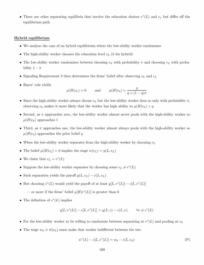
� There are other separating equilibria that involve the education choices e∗(L) and es but differ off the
equilibrium path
Hybrid equilibrium
� We analyze the case of an hybrid equilibrium where the low-ability worker randomizes
� The high-ability worker chooses the education level eh (h for hybrid)
� The low-ability worker randomizes between choosing eh with probability π and choosing eL with proba-
bility 1− π
� Signaling Requirement 3 then determines the firms’ belief after observing eh and eL
� Bayes’ rule yields
µ(H|eL) = 0 and µ(H|eh) =q
q + (1− q)π
� Since the high-ability worker always choose eh but the low-ability worker does so only with probability π,
observing eh makes it more likely that the worker has high ability so µ(H|eh) > q
� Second, as π approaches zero, the low-ability worker almost never pools with the high-ability worker so
µ(H|eh) approaches 1
� Third, as π approaches one, the low-ability worker almost always pools with the high-ability worker so
µ(H|eh) approaches the prior belief q
� When the low-ability worker separates from the high-ability worker by choosing eL
� The belief µ(H|eL) = 0 implies the wage w(eL) = y(L, eL)
� We claim that eL = e∗(L)
� Suppose the low-ability worker separates by choosing some eL 6= e∗(L)
� Such separation yields the payoff y(L, eL)− c(L, eL)
� But choosing e∗(L) would yield the payoff of at least y[L, e∗(L)] − c[L, e∗(L)]
– or more if the firms’ belief µ[H|e∗(L)] is greater than 0
� The definition of e∗(L) implies
y[L, e∗(L)]− c[L, e∗(L)] > y(L, e)− c(L, e), ∀e 6= e∗(L)
� For the low-ability worker to be willing to randomize between separating at e∗(L) and pooling at eh
� The wage wh ≡ w(eh) must make that worker indifferent between the two
w∗(L)− c[L, e∗(L)] = wh − c(L, eh) (P)
160
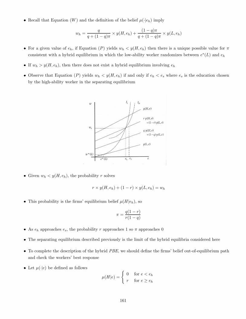
� Recall that Equation (W ) and the definition of the belief µ(·|eh) imply
wh =q
q + (1− q)π× y(H, eh) +
(1− q)π
q + (1− q)π× y(L, eh)
� For a given value of eh, if Equation (P ) yields wh < y(H, eh) then there is a unique possible value for π
consistent with a hybrid equilibrium in which the low-ability worker randomizes between e∗(L) and eh
� If wh > y(H, eh), then there does not exist a hybrid equilibrium involving eh
� Observe that Equation (P ) yields wh < y(H, eh) if and only if eh < es where es is the education chosen
by the high-ability worker in the separating equilibrium
� Given wh < y(H, eh), the probability r solves
r × y(H, eh) + (1− r)× y(L, eh) = wh
� This probability is the firms’ equilibrium belief µ(H|eh), so
π =q(1− r)
r(1− q)
� As eh approaches es, the probability r approaches 1 so π approaches 0
� The separating equilibrium described previously is the limit of the hybrid equilibria considered here
� To complete the description of the hybrid PBE, we should define the firms’ belief out-of-equilibrium path
and check the workers’ best response
� Let µ(·|e) be defined as follows
µ(H|e) ={
0 for e < eh
r for e ≥ eh
161
� The firms’ strategy is then
w(e) =
{
y(L, e) for e < eh
r × y(L, e) + (1− r)× y(H, e) for e ≥ eh
� It remains to check that the workers’ strategy
– e(L) = eh with probability π and e(L) = e∗(L) with probability 1− π
– e(H) = eh
is a best response to the firms’ strategy
Corporate investment and capital structure
� Consider an entrepreneur who has started a company but needs outside financing to undertake an attrac-
tive new project
� The entrepreneur has private information about the profitability of the existing company
� The payoff of the new project cannot be disentangled from the payoff of the existing company
� All that can be observed is the aggregate profit of the firm
� Suppose the entrepreneur offers a potential investor an equity stake in the firm in exchange for the
necessary financing
� Under what circumstances will the new project be undertaken?
� What will the equity stake be?
� Suppose that the profit of the existing company can be either high or low: π ∈ {H,L} with H > L > 0
� The potential investor’s opportunity cost is r, i.e., there is an alternative investment possibility with rate
of return r
� The required investment in the new project is I
� The payoff will be R
� The new project is attractive in the sense that the NPV is positive, i.e., R > I(1 + r)
The timing and the payoffs of the game are:
1. Nature determines the profit of the existing company
� The probability that π = L is p
162
2. The entrepreneur learns π and then offers the potential investor an equity stake s, where 0 ≤ s ≤ 1
3. The investor observes s but not π and then decides either to accept or to reject the offer
4. Payoffs:
� If the investor rejects the offer then the investor’s payoff is I(1 + r) and the entrepreneur’s payoff is
π
� If the investor accepts s then the investor’s payoff is s(π+R) and the entrepreneur’s is (1−s)(π+R)
� Suppose that after receiving the offer s the investor believes that the probability that π = L is q(s)
� Then the investor will accept s if and only if
s[qL+ (1− q)H +R] ≥ I(1 + r) (PC-I)
� Suppose the profit of the existing company is π
� The entrepreneur prefers to receive the financing at the cost of an equity stake of s if and only if
s ≤ R
π +R(PC-E)
� In a pooling PBE, the investor’s belief must be q(spo) = p after receiving the equilibrium offer spo
� The participation constraint (PC − E) is more difficult to satisfy for π = H than for π = L
� Therefore, a pooling equilibrium (with “accepts” as an action) exists only if
I(1 + r)
pL+ (1− p)H +R≤ R
H +R(NC-p)
� If p is close enough to zero, (NC-p) holds because R > I(1 + r)
� If p is close enough to one, however, the necessary condition (NC-p) holds only if
R− I(1 + r) ≥ I(1 + r)
RH − L (sNC-p)
� In a pooling equilibrium, the high-profit type must subsidize the low-profit type
� Setting q(spo) = p yields that the investor accepts to finance the project if and only if
spo ≥ I(1 + r)
pL+ (1− p)H +R>
I(1 + r)
H +R
� If the investor were certain that π = H the he would accept the smaller equity stake
ssyH =I(1 + r)
H +R
163

� The larger equity stake required in a pooling equilibrium may be so expensive that the high-profit firm
would prefer to forego the new project
� A pooling equilibrium exists if p is close to zero, so that the cost of subsidization is small
� Or if the profit from the new project outweighs the cost of subsidization
� If (NC-p) fails then a pooling equilibrium does not exist
� A separating equilibrium always exists, however
� The low-profit type offers
sL =I(1 + r)
L+R
which the investor accepts
� The high-profit type offers
sH <I(1 + r)
H +R
and the investor rejects
� In such an equilibrium, investment is inefficiently low: the new project is certain to be profitable, but the
high-profit type foregoes the investment
� There is no way for the high-profit type to distinguish itself
� Financing terms that are attractive to the high-profit type are even more attractive to the low-profit type
� As Myers and Majluf (J. Fin. Econ. 1984) observes, the forces in this model push firms toward either
debt or internal sources of funds
� Actually, Myers and Majluf analyze a large firm (with shareholders and a manager) rather than an
entrepreneur (who is both the manager and the sole shareholder)
� We consider the possibility that the entrepreneur can offer debt as well as equity
� Suppose the investor accepts the debt contract D
� If the entrepreneur does not declare bankruptcy then the investor’s payoff is D and the entrepreneur’s is
π +R−D
� If the entrepreneur does declare bankruptcy then the investor’s payoff is π +R and the entrepreneur’s is
zero
� Since L > 0, there is always a pooling equilibrium: both profit-types offer the debt contract D = I(1+ r),
which the investor accepts
� If L were sufficiently negative that R + L < I(1 + r), then the low-profit type could not repay this debt
so the investor would not accept the contract
164
� A similar argument would apply if L and H represented expected rather than certain profits
� Suppose that the type π means that the existing company’s profit will be
– π +K with probability 1/2
– π −K with probability 1/2
� If L−K + R < I(1 + r) then there is probability 1/2 that the low profit type will not be able to repay
the debt D = I(1 + r) so the investor will not accept the contract
Monetary policy
� Consider a sequential-move game in which employers and workers negotiate nominal wages
� After the negotiation, the monetary authority chooses the money supply, which in turn determines the
rate of inflation
� If wage contracts cannot be perfectly indexed, employers and workers will try to anticipate inflation in
setting the wage
� Once an imperfectly indexed nominal wage has been set, actual inflation above the anticipated level of
inflation will erode the real wage
� This causes employers to expand employment and output
� The monetary authority therefore faces a trade-off between the costs of inflation and the benefits of
reduced unemployment and increased output that follow from surprise inflation
We follow Barro and Gordon (J. Mon. Econ. 1983) and analyzed a reduced-form version of this model in the
following game
� First, employers form an expectation of inflation, πe
� Second, the monetary authority observes this expectation and chooses actual inflation, π
� The payoff to employers is −(π−πe)2: employers simply want to anticipate inflation correctly, they achieve
their maximum payoff when π = πe
� The monetary authority would like inflation to be zero but output (y) to be at its efficient level (y∗)
� The payoff to the monetary authority is
U(π, y) = −cπ2 − (y − y∗)2
where the parameter c > 0 reflects the monetary authority’s trade-off between its two goals
165
� Suppose the actual output is the following function of target output and surprise inflation
y(π, πe) = by∗ + d(π − πe)
– Where b < 1 reflects the presence of monopoly power in product markets
– If there is no surprise inflation, π = πe, then actual output will be smaller than would be efficient
– Where d > 0 measures the effect of surprise inflation on output through real wages
� We can then rewrite the monetary authority’s payoff as
W (π, πe) = U(π, y(π, πe)) = −cπ2 − [(b− 1)y∗ + d(π − πe)]2
� We propose to solve the subgame-perfect outcome of this game
� We first compute the monetary authority’s optimal choice of π given employers’ expectation πe:
π∗(πe) =d
c+ d2[(1− b)y∗ + dπe]
� Since employers anticipate that the monetary authority will choose π∗(πe), employers choose πe to maxi-
mize −[π∗(πe)− πe]2, which yields π∗(πe) = πe, or
πe =d(1− b)
cy∗ ≡ πs
� In this subgame-perfect outcome, the monetary authority is expected to inflate and does so
� We consider a two-period version of the previous model and we add private information
� In the two-period model, each player’s payoff is the sum of the player’s one-period payoffs
W (π1, πe1) +W (π2, π
e2) and − (π1 − πe
1)2 − (π2 − πe
2)2
where πt is actual inflation in period t and πet is employers’ expectation (at end of period t−1 or beginning
of period t) of inflation in period t
� We now assume that the parameter c is privately known by the monetary authority: c ∈ {S,W}
– c = S or W for “strong” and “weak” at fighting inflation where S > W > 0
1. Nature draws the monetary authority’s type, c
� The probability that c = W is p
2. Employers form πe1, their expectation of first-period inflation
3. The monetary authority observes πe1 and then chooses actual first-period inflation, π1
4. Employers observe π1 but not c, and then form πe2, their expectation of second-period inflation
166
5. The monetary authority observes πe2 and then chooses actual second-period inflation, π2
� There is a one-period signaling game embedded in this two-period monetary-policy game
� The Sender’s message is the monetary authority’s first-period choice of inflation, π1
� The Receiver’s action is employers’ second-period expectation of inflation, πe2
� Employers’ first-period expectation of inflation and the monetary authority’s second-period choice of
inflation precede and follow the signaling game
� If the monetary authority’s type is c then its optimal choice of π2 given the expectation πe2 is
π∗2(π
e2, c) ≡
d
c+ d2[(1− b)y∗ + dπe
2]
� Employers anticipate this
� If employers begin the second period believing that the probability that c = W is q, then they will form
the expectation πe2(q) that maximizes
−q[π∗2(π
e2,W )− πe
2]2 − (1− q)[π∗
2(πe2, S)− πe
2]2
Monetary policy: pooling equilibrium
� In a pooling equilibrium, both types choose the same first-period inflation π∗1
� Employers’ first-period expectation is πe1 = π∗
1
� On the equilibrium path, employers begin the second period believing that the probability that c = W is
p and so form the expectation πe2(p)
� Then the monetary authority of type c chooses its optimal second-period inflation given this expectation,
namely π∗2 [π
e2(p), c], thus ending the game
Monetary policy: separating equilibrium
� In a separating equilibrium, the two types choose different first-period inflation levels, say πW and πS
� So employers’ first-period expectation is πe1 = pπW + (1− p)πS
� After observing πW , employers begin the second period believing that c = W and so form the expectation
πe2(1) solution of the equation
πe2 = π∗
2(πe2(1),W ) i.e., πe
2(1) =d(1 − b)
Wy∗
� Likewise, observing πS leads to
πe2(0) =
d(1− b)
Sy∗
167
� In equilibrium, the weak type then chooses π∗2 [π
e2(1),W ] and the strong type π∗
2[πe2(0), S], ending the game
To complete the description of the such an equilibrium it remains
1. to specify the Receiver’s out-of-equilibrium beliefs and actions
2. to check that no Sender-type has an incentive to deviate
3. in particular, to check neither type has an incentive to mimic the other’s equilibrium behavior
� The weak-type might be tempted to choose πS in the first period, thereby inducing πe2(0) as the employers’
second-period expectation
� And then choose π∗2[π
e2(0),W ] to end the game
� Even if πS is uncomfortably low for the weak type, the ensuing expectation πe2(0) might be so low that
the weak type receives a huge payoff from the unanticipated inflation
π∗2 [π
e2(0),W ]− πe
2(0)
� In a separating equilibrium, the strong type’s first period inflation must be low enough that the weak
type is not tempted to mimic the strong type
� In spite of the subsequent benefit from unanticipated second-period inflation
4.3 Other applications of Signaling Games
Cheap-Talk games
� Cheap-talk games are analogous to signaling games
� But the Sender’s messages are just talk: costless, non-binding, non-verifiable claims
� Such talk cannot be informative in Spence’s job market signaling game:
– a worker who simply announced “My ability is high” would not be believed
� In other contexts, cheap talk can be informative
� Stein (Am. Econ. Rev. 1989) shows that policy announcements by the Federal Reserve can be informative
but cannot be too precise
� Matthews (Quarterly J. Econ. 1989) studies how a veto threat by the president can influence which bill
gets through Congress
� One can also ask how to design environments to take advantage of cheap talk
� Austen-Smith (1990): muito interessante!!
shows that in some settings debate among self-interested legislators improves the social value of the
eventual legislation
168
� Farrell and Gibbons (1991) show that in some settings unionization improves social welfare because it
facilitates communication from the work force to management
� In Spence’s job market model, cheap talk cannot be informative because all the Sender’s types have the
same preferences over the Receiver’s possible actions:
– all workers prefer higher wages, independent of ability
� Let’s illustrate why uniformity of preferences over the Receiver’s possible actions vitiates cheap talk
� Suppose there were a pure-strategy equilibrium in which one subset of Sender-types, T1, send one message,
m1
� While another subset of types, T2, sends another message, m2
� In equilibrium, the Receiver will interpret mi as coming from Ti and so will take the optimal action given
this belief; denote this action by ai
� Since all Sender-type have the same preferences over actions
– If one type prefers a1 to a2 , then all types have this preference and will send m1 rather than m2
� This destroys the putative equilibrium
There are 3 necessary conditions for cheap talk to be informative
1. different Sender-types have different preferences over the Receiver’s actions
2. the Receiver prefers different actions depending on the Sender’s type
3. Receiver’s preferences over actions not be completely opposed to the Sender’s preferences
� Suppose that the Receiver prefers low actions when the Sender’s type is low and high actions when
the Sender’s type is high
� If low Sender-types prefer low actions and high types high actions, then communication can occur
� If the Sender has the opposite preference then communication cannot occur because the Sender would
like to mislead the Receiver
� Crawford and Sobel (Econometrica 1982) analyze an abstract model that satisfies these three necessary
conditions: they show that
– more communication can occur through cheap talk when the players’ preferences are more closely
aligned
– perfect communication cannot occur unless the players’ preferences are perfectly aligned
� Each of economic applications (cheap talk of the Fed, veto threats, information transmission in debate,
union voice) involve complicated models of economic environments
� We will only analyze abstract cheap-talk games
169
An abstract cheap-talk game
The timing of the simplest cheap-talk game is identical to the timing of a signaling game; only payoffs differ
1. Nature draws a type ti for the Sender from a set T = {t1, ..., tI} of feasible types according to a probability
distribution p with full support, i.e., p(t) > 0 for every t ∈ T
2. The Sender observes ti and then chooses a message mj from a set of feasible messages M = {m1, ...,mJ}
3. The Receiver observes mj (but not ti) and then chooses an action ak from a set of feasible actions
A = {a1, ..., ak}
4. Payoffs are given by US(ti, ak) and UR(ti, ak)
� The key feature of such a game is that the message has no direct effect on either the Sender’s or the
Receiver’s payoff
� The only way the message can matter is through its information content
� By changing the Receiver’s belief about the Sender’s type, a message can change the Receiver’s action
� And thus, indirectly affect both players’ payoffs
� We will assume that anything can be said in the sense that M = T
� Because the simplest cheap-talk and signaling games have the same timing, the definitions of PBE in the
two games are identical
� A pure-strategy PBE is a pair of strategies m∗ : T → M and a∗ : M → A, and a family (µ(·|mj))mj∈M
of beliefs over T satisfying Requirements (1), (2R), (2S) and (3)
� In a cheap-talk game, a pooling equilibrium always exists
� Because messages have no direct effect on the Sender’s payoff
� If the Receiver will ignore all messages then pooling is a best response for the Sender; and if the Sender
is pooling then a best response for the Receiver is to ignore all messages
� More formally, let a denote the Receiver’s optimal action in a pooling equilibrium, i.e., a solves
maxak∈A
∑
ti∈T
p(ti)UR(ti, ak)
� Define a∗ by a∗(mj) = a for every mj ∈ M
� Fix an arbitrary message m in M and define m∗ by m∗(ti) = m for every ti ∈ T
� Let µ(·|ti) = p for every ti ∈ T
� This is a pooling equilibrium
170
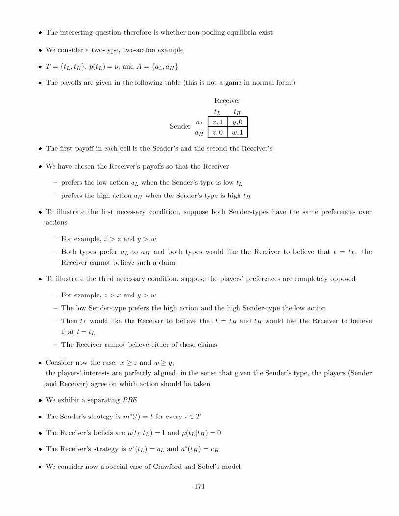
� The interesting question therefore is whether non-pooling equilibria exist
� We consider a two-type, two-action example
� T = {tL, tH}, p(tL) = p, and A = {aL, aH}
� The payoffs are given in the following table (this is not a game in normal form!)
Sender
Receiver
tL tH
aL x, 1 y, 0
aH z, 0 w, 1
� The first payoff in each cell is the Sender’s and the second the Receiver’s
� We have chosen the Receiver’s payoffs so that the Receiver
– prefers the low action aL when the Sender’s type is low tL
– prefers the high action aH when the Sender’s type is high tH
� To illustrate the first necessary condition, suppose both Sender-types have the same preferences over
actions
– For example, x > z and y > w
– Both types prefer aL to aH and both types would like the Receiver to believe that t = tL: the
Receiver cannot believe such a claim
� To illustrate the third necessary condition, suppose the players’ preferences are completely opposed
– For example, z > x and y > w
– The low Sender-type prefers the high action and the high Sender-type the low action
– Then tL would like the Receiver to believe that t = tH and tH would like the Receiver to believe
that t = tL
– The Receiver cannot believe either of these claims
� Consider now the case: x ≥ z and w ≥ y;
the players’ interests are perfectly aligned, in the sense that given the Sender’s type, the players (Sender
and Receiver) agree on which action should be taken
� We exhibit a separating PBE
� The Sender’s strategy is m∗(t) = t for every t ∈ T
� The Receiver’s beliefs are µ(tL|tL) = 1 and µ(tL|tH) = 0
� The Receiver’s strategy is a∗(tL) = aL and a∗(tH) = aH
� We consider now a special case of Crawford and Sobel’s model
171
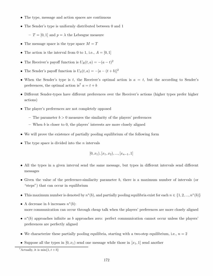
� The type, message and action spaces are continuous
� The Sender’s type is uniformly distributed between 0 and 1
– T = [0, 1] and p = λ the Lebesgue measure
� The message space is the type space M = T
� The action is the interval from 0 to 1, i.e., A = [0, 1]
� The Receiver’s payoff function is UR(t, a) = −(a− t)2
� The Sender’s payoff function is US(t, a) = −[a− (t+ b)]2
� When the Sender’s type is t, the Receiver’s optimal action is a = t, but the according to Sender’s
preferences, the optimal action is7 a = t+ b
� Different Sender-types have different preferences over the Receiver’s actions (higher types prefer higher
actions)
� The player’s preferences are not completely opposed
– The parameter b > 0 measures the similarity of the players’ preferences
– When b is closer to 0, the players’ interests are more closely aligned
� We will prove the existence of partially pooling equilibrium of the following form
� The type space is divided into the n intervals
[0, x1), [x1, x2), ..., [xn−1, 1]
� All the types in a given interval send the same message, but types in different intervals send different
messages
� Given the value of the preference-similarity parameter b, there is a maximum number of intervals (or
“steps”) that can occur in equilibrium
� This maximum number is denoted by n∗(b), and partially pooling equilibria exist for each n ∈ {1, 2, ..., n∗(b)}
� A decrease in b increases n∗(b):
more communication can occur through cheap talk when the players’ preferences are more closely aligned
� n∗(b) approaches infinite as b approaches zero: perfect communication cannot occur unless the players’
preferences are perfectly aligned
� We characterize these partially pooling equilibria, starting with a two-step equilibrium, i.e., n = 2
� Suppose all the types in [0, x1) send one message while those in [x1, 1] send another
7Actually, it is min{1, t+ b}
172
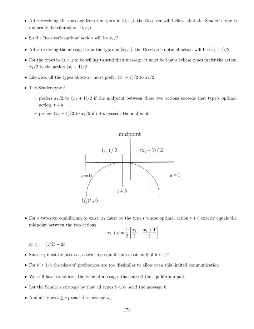
� After receiving the message from the types in [0, x1), the Receiver will believe that the Sender’s type is
uniformly distributed on [0, x1)
� So the Receiver’s optimal action will be x1/2
� After receiving the message from the types in [x1, 1], the Receiver’s optimal action will be (x1 + 1)/2
� For the types in [0, x1) to be willing to send their message, it must be that all these types prefer the action
x1/2 to the action (x1 + 1)/2
� Likewise, all the types above x1 must prefer (x1 + 1)/2 to x1/2
� The Sender-type t
– prefers x1/2 to (x1 + 1)/2 if the midpoint between these two actions exceeds that type’s optimal
action, t+ b
– prefers (x1 + 1)/2 to x1/2 if t+ b exceeds the midpoint
� For a two-step equilibrium to exist, x1 must be the type t whose optimal action t+ b exactly equals the
midpoint between the two actions
x1 + b =1
2
[x12
+x1 + 1
2
]
or x1 = (1/2) − 2b
� Since x1 must be positive, a two-step equilibrium exists only if b < 1/4
� For b ≥ 1/4 the players’ preferences are too dissimilar to allow even this limited communication
� We still have to address the issue of messages that are off the equilibrium path
� Let the Sender’s strategy be that all types t < x1 send the message 0
� And all types t ≥ x1 send the message x1
173
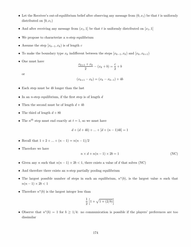
� Let the Receiver’s out-of-equilibrium belief after observing any message from (0, x1) be that t is uniformly
distributed on [0, x1)
� And after receiving any message from (x1, 1] be that t is uniformly distributed on [x1, 1]
� We propose to characterize a n-step equilibrium
� Assume the step [xk−1, xk) is of length c
� To make the boundary type xk indifferent between the steps [xk−1, xk) and [xk, xk+1)
� One must havexk+1 + xk
2− (xk + b) =
c
2+ b
or
(xk+1 − xk) = (xk − xk−1) + 4b
� Each step must be 4b longer than the last
� In an n-step equilibrium, if the first step is of length d
� Then the second must be of length d+ 4b
� The third of length d+ 8b
� The nth step must end exactly at t = 1, so we must have
d+ (d+ 4b) + ...+ [d+ (n− 1)4b] = 1
� Recall that 1 + 2 + ...+ (n− 1) = n(n− 1)/2
� Therefore we have
n× d+ n(n− 1)× 2b = 1 (NC)
� Given any n such that n(n− 1)× 2b < 1, there exists a value of d that solves (NC)
� And therefore there exists an n-step partially pooling equilibrium
� The largest possible number of steps in such an equilibrium, n∗(b), is the largest value n such that
n(n− 1)× 2b < 1
� Therefore n∗(b) is the largest integer less than
1
2
[
1 +√
1 + (2/b)]
� Observe that n∗(b) = 1 for b ≥ 1/4: no communication is possible if the players’ preferences are too
dissimilar
174
� Moreover, n∗(b) approaches infinity only as b approaches zero: perfect communication cannot occur unless
the players’ preferences are perfectly aligned
Sequential bargaining under asymmetric information
� Consider a firm and a union bargaining over wages
� For simplicity, assume that employment is fixed
� The amount that union members earn if not employed, called union’s reservation wage, is denoted by wr
� The firm’s profit, denoted by π, is uniformly distributed on [πL, πH ]
� The value of π is privately known by the firm
– The firm might have superior knowledge concerning new products in the planning stage
� We simplify the analysis by assuming that wr = πL = 0
The bargaining game lasts at most two periods
1. In the first period, the union makes a wage offer, w1
� If the firm accepts this offer then the game ends
� The union’s payoff is w1 and the firm’s is π − w1
� These payoffs are the present values of the wage and (net) profit streams that accrue to the players
over the life of the contract being negotiated
2. If the firm rejects this offer the game proceeds to the second period
� The union makes a second wage offer, w2
� If the firm accepts this offer then the present values of the players’ payoffs are δw2 for the union and
δ(π − w2) for the firm
� δ reflects both discounting and the reduced life of the contract remaining after the first period
� If the firm rejects the union’s second offer then the game ends and payoffs are zero for both players
� A more realistic model might allow the bargaining to continue until an offer is accepted
� Or might force the parties to submit to binding arbitration after a prolonged strike
� Here we sacrifice realism for tractability
� We refer to Sobel adn Takahashi (Rev. Econ. Sud. 1983) for an infinite horizon analysis
175
We begin by sketching the unique PBE of this game
� The union’s first-period wage offer is
w∗1 =
(2− δ)2
2(4 − 3δ)πH
� If the firm’s profit, π, exceeds
π∗1 =
2w∗1
2− δ=
2− δ
4− 3δπH
then the firm accepts w∗1; otherwise the firm rejects w∗
1
� If its first-period offer is rejected, the union updates its belief about the firm’s profit
– The union believes that π is uniformly distributed on [0, π∗1 ]
� The union’s second-period wage offer (conditional on w1 being rejected) is
w∗2 =
π∗1
2=
2− δ
2(4− 3δ)πH < w∗
1
� If the firm’s profit, π, exceeds w∗2 then the firm accepts the offer; otherwise, it rejects it
� We will refer interchangeably to one firm with many possible profit types and to many firms each with
its own profit level
� In each period, high-profits firms accept the union’s offer
� While low-profit firms reject it
� The union’s second-period belief reflects the fact that high-profit firms accepted the first-period offer
� In equilibrium, low-profit firms tolerate a one-period strike in order to convince the union that they are
low-profit and so induce the union to offer a lower second-period wage
� Firms with very low profits find even the lower second-period offer intolerably high and so reject it, too
� We propose an extensive-form representation of a simplified version of the game
� There are only two values of π: πL and πH
� The union has only two possible wage offers wL and wH
� In this simplified game, the union has the move at three information sets: the union’s strategy consists
of three wage offers
1. The first-period offer, w1
2. The second-period offer, w2(H) after w1 = wH is rejected
3. The second-period offer, w2(L) after w1 = wL is rejected
176
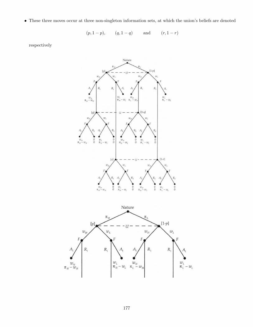
� These three moves occur at three non-singleton information sets, at which the union’s beliefs are denoted
(p, 1− p), (q, 1 − q) and (r, 1− r)
respectively
177
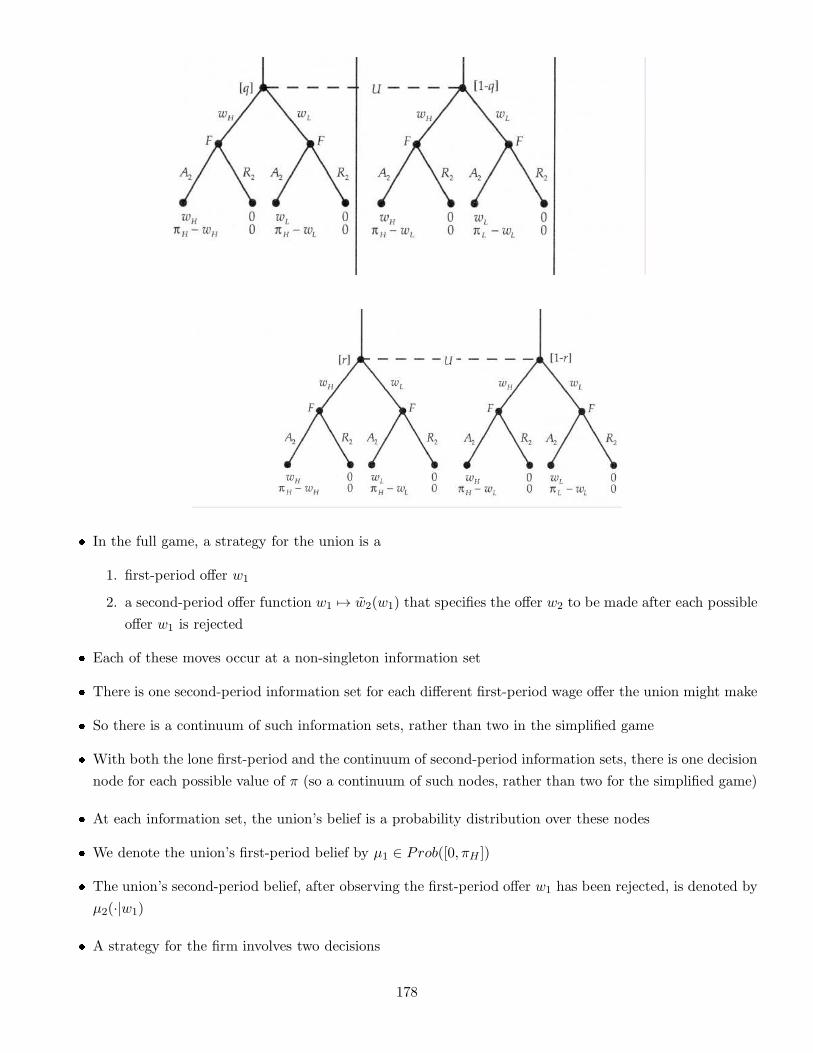
� In the full game, a strategy for the union is a
1. first-period offer w1
2. a second-period offer function w1 7→ w2(w1) that specifies the offer w2 to be made after each possible
offer w1 is rejected
� Each of these moves occur at a non-singleton information set
� There is one second-period information set for each different first-period wage offer the union might make
� So there is a continuum of such information sets, rather than two in the simplified game
� With both the lone first-period and the continuum of second-period information sets, there is one decision
node for each possible value of π (so a continuum of such nodes, rather than two for the simplified game)
� At each information set, the union’s belief is a probability distribution over these nodes
� We denote the union’s first-period belief by µ1 ∈ Prob([0, πH ])
� The union’s second-period belief, after observing the first-period offer w1 has been rejected, is denoted by
µ2(·|w1)
� A strategy for the firm involves two decisions
178
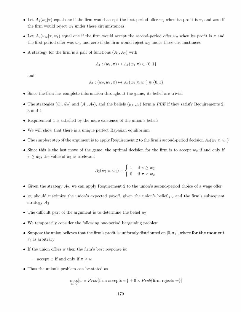
� Let A1(w1|π) equal one if the firm would accept the first-period offer w1 when its profit is π, and zero if
the firm would reject w1 under these circumstances
� Let A2(ww|π,w1) equal one if the firm would accept the second-period offer w2 when its profit is π and
the first-period offer was w1, and zero if the firm would reject w2 under these circumstances
� A strategy for the firm is a pair of functions (A1, A2) with
A1 : (w1, π) 7→ A1(w1|π) ∈ {0, 1}
and
A1 : (w2, w1, π) 7→ A2(w2|π,w1) ∈ {0, 1}
� Since the firm has complete information throughout the game, its belief are trivial
� The strategies (w1, w2) and (A1, A2), and the beliefs (µ1, µ2) form a PBE if they satisfy Requirements 2,
3 and 4
� Requirement 1 is satisfied by the mere existence of the union’s beliefs
� We will show that there is a unique perfect Bayesian equilibrium
� The simplest step of the argument is to apply Requirement 2 to the firm’s second-period decision A2(w2|π,w1)
� Since this is the last move of the game, the optimal decision for the firm is to accept w2 if and only if
π ≥ w2; the value of w1 is irrelevant
A2(w2|π,w1) =
{
1 if π ≥ w2
0 if π < w2
� Given the strategy A2, we can apply Requirement 2 to the union’s second-period choice of a wage offer
� w2 should maximize the union’s expected payoff, given the union’s belief µ2 and the firm’s subsequent
strategy A2
� The difficult part of the argument is to determine the belief µ2
� We temporarily consider the following one-period bargaining problem
� Suppose the union believes that the firm’s profit is uniformly distributed on [0, π1], where for the moment
π1 is arbitrary
� If the union offers w then the firm’s best response is:
– accept w if and only if π ≥ w
� Thus the union’s problem can be stated as
maxw≥0
[w × Prob{firm accepts w}+ 0× Prob{firm rejects w}]
179
where
Prob{firm accepts w} =π1 − w
π1
� The optimal wage offer is therefore w∗(π1) = π1/2
� We return (permanently) to the two-period problem
� Assume that the union offers w1 in the first period and the firm expects the union to offer w2 in the
second period
� The firm’s possible payoffs are
– π − w − 1 from accepting w1
– δ(π − w2) from rejecting w1 and accepting w2
– zero from rejecting both offers
� The firm prefers accepting w1 to accepting w2 if π −w1 ≥ δ(π − w2), or
π ≥ w1 − δw2
1− δ≡ π∗(w1, w2)
� And the firm prefers accepting w1 to rejecting both offers if π − w1 ≥ 0
� Thus for arbitrary values of w1 and w2, firms with π ≥ max{π∗(w1, w2), w1} will accept w1 and the other
firms will reject
� Since Requirement 2 dictates that the firm act optimally given the players’ subsequent strategies, we can
derive A1(w1|π) by replacing the arbitrary wage w2 by w2(w1), i.e.,
A1(w1|π) ={
1 if π ≥ max{π∗(w1, w2(w1)), w1}0 if π < max{π∗(w1, w2(w1)), w1}
� We can derive µ2, the union’s second-period belief at the information set reached if the first period offer
w1 is rejected
� Requirement 4 dictates that the union’s belief be determined by Bayes’ rule and the firm’s strategy
� Thus, given the first part of the firm’s strategy A1 just derived
� The union’s belief must be that the types remaining in the second period are uniformly distributed on
[0, π1(w1, w2)] where
π1(w1, w2) ≡ max{π∗(w1, w2(w1)), w1}
� Given this belief, the union’s optimal second-period offer must be
w2(w1) = w∗(π1(w1, w2)) =π1(w1, w2)
2
180
� It follows that w2(w1) solves the implicit equation for w2 as a function of w1:
2w2 = max{π∗(w1, w2), w1}
� To solve this equation, suppose that w1 ≥ π∗(w1, w2)
� Then 2w2 = w1 but this contradicts w1 ≥ π∗(w1, w2)
� Therefore, we must have 2w2 = π∗(w1, w2) implying that
w2(w1) =w1
2− δ
� Therefore, the union’s second-period belief at the information set reached if the first period offer w1 is
rejected
� Is that the types remaining in the second period are uniformly distributed on
[0, π(w1)] where π(w1) = π1(w1, w2(w1))
� Since w2(w1) = w1/(2 − δ) we get that
π(w1) =2w1
2− δ
� We have now reduced the game to a single-period optimization problem for the union
� Given the union’s first-period wage offer, w1, we have specified
– the firm’s optimal first-period response
A1(w1|π) = 1 ⇔ π ≥ π(w1) =2w1
2− δ
– the union’s belief entering the second period
µ2(·|w1) =1
π(w1)λ[0,π(w1))
– the union’s optimal second-period offer
w2(w1) =w1
2− δ
– the firm’s optimal second-period response
A2(w2|π,w1) = 1 ⇔ π ≥ w2
� Thus, the union’s first-period wage offer w1 should be chosen to solve
w1 × µ1{A1(w1|·) = 1}+Π2(π1)× [1− µ1{A1(w1|·) = 1}]
181
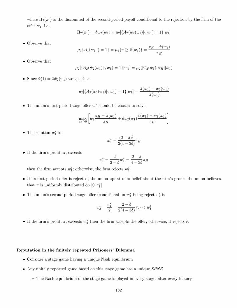
where Π2(π1) is the discounted of the second-period payoff conditional to the rejection by the firm of the
offer w1, i.e.,
Π2(π1) = δw2(w1)× µ2[{A2(w2(w1)|·, w1) = 1}|w1]
� Observe that
µ1{A1(w1|·) = 1} = µ1{π ≥ π(w1)} =πH − π(w1)
πH
� Observe that
µ2[{A2(w2(w1)|·, w1) = 1}|w1] = µ2([w2(w1), πH ]|w1)
� Since π(1) = 2w2(w1) we get that
µ2[{A2(w2(w1)|·, w1) = 1}|w1] =π(w1)− w2(w1)
π(w1)
� The union’s first-period wage offer w∗1 should be chosen to solve
maxw1≥0
[
w1πH − π(w1)
πH+ δw2(w1)
π(w1)− w2(w1)
πH
]
� The solution w∗1 is
w∗1 =
(2− δ)2
2(4 − 3δ)πH
� If the firm’s profit, π, exceeds
π∗1 =
2
2− δw∗1 =
2− δ
4− 3δπH
then the firm accepts w∗1; otherwise, the firm rejects w∗
1
� If its first period offer is rejected, the union updates its belief about the firm’s profit: the union believes
that π is uniformly distributed on [0, π∗1 ]
� The union’s second-period wage offer (conditional on w∗1 being rejected) is
w∗2 =
π∗1
2=
2− δ
2(4− 3δ)πH < w∗
1
� If the firm’s profit, π, exceeds w∗2 then the firm accepts the offer; otherwise, it rejects it
Reputation in the finitely repeated Prisoners’ Dilemma
� Consider a stage game having a unique Nash equilibrium
� Any finitely repeated game based on this stage game has a unique SPNE
– The Nash equilibrium of the stage game is played in every stage, after every history
182

� A great deal of experimental evidence suggests that cooperation occurs frequently during finitely repeated
Prisoners’ Dilemmas
� Especially in stages that are not too close to the end
� Kreps, Milgrom, Roberts, and Wilson (J. Econ. Theory 1982) show that a reputation model offers an
explanation of this evidence
� We introduce a new way of modeling asymmetric information
� Rather than assume that one player has private information about his or her payoffs
� We will assume that the player has private information about his or her feasible strategies
� We will assume that with probability p the Row player can play only the Tit-for-Tat strategy
– This strategy begins the repeated game by cooperating and thereafter mimics the opponent’s previous
play
� While with probability 1 − p the Row player can play any of the strategies available in the complete-
information repeated game (including Tit-for-Tat)
– This Row-type is called “rational”
� Under this formulation, if the Row player ever deviates from the Tit-for-Tat strategy then it becomes
common knowledge that Row is rational
� The spirit of KMRW’s analysis is that even if p is very small
– i.e., even if the Column player has only a tiny suspicion that the Row player might not be rational
� This uncertainty can have a big effect
� KMRW show that there is an upper bound on the number of stages in which either player finks in
equilibrium
� This upper bound depends on p and on the stage-game payoffs but not on the number of stages in the
repeated game
� Thus, in any equilibrium of a long enough repeated game, the fraction of stages in which both players
cooperate is large
The two key steps in KMRW’s argument are
1. If the Row player deviates from Tit-for-Tat then it becomes common knowledge that Row is rational
� So neither player cooperates thereafter
� So the rational Row has an incentive to mimic Tit-for-Tat
183

2. Given an assumption on the stage-game payoffs to be imposed below, the Column player’s best response
against Tit-for-Tat would be to cooperate until the last stage of the game
� We will consider the complement of the analysis in KMRW
� Rather than assume that p is small and analyze long repeated games
� We will assume that p is large enough that there exists an equilibrium in which both players cooperate in
all but the last two stages of a (possibly short) repeated game
� We begin with the two period case
The timing is
1. Nature draws a type for the Row player
� With probability p, Row has only the Tit-for-Tat strategy available
� With probability 1− p, Row can play any strategy
� Row learns his or her type, but Column does not learn Row’s type
2. Row and Column play the Prisoners’ Dilemma
� The players’ choices in this stage game become common knowledge
3. Row and Column play the Prisoners’ Dilemma for a second and last time
4. Payoffs are received
� The playoffs are the (undiscounted) sums of their stage-game payoffs
Row
Column
Cooperate Fink
Cooperate 1, 1 b, a
Fink a, b 0, 0
� To make this stage game a Prisoners’ Dilemma, we assume that
a > 1 and b < 0
� Recall that finking (F) strictly dominates cooperating (C) in the stage game, both for rational Row and
for Column
� Since, in the last stage of this two-period game of incomplete information, Column will surely fink
� Then, there is no reason for the rational Row to cooperate in the first stage
� Tit-for-Tat begins the game by cooperating
� Thus, the only move to be determined is Column’s first-period move (X)
184
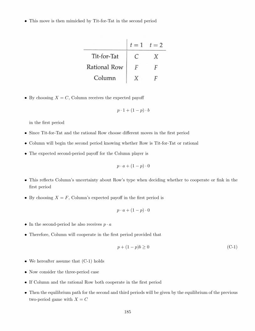
� This move is then mimicked by Tit-for-Tat in the second period
� By choosing X = C, Column receives the expected payoff
p · 1 + (1− p) · b
in the first period
� Since Tit-for-Tat and the rational Row choose different moves in the first period
� Column will begin the second period knowing whether Row is Tit-for-Tat or rational
� The expected second-period payoff for the Column player is
p · a+ (1− p) · 0
� This reflects Column’s uncertainty about Row’s type when deciding whether to cooperate or fink in the
first period
� By choosing X = F , Column’s expected payoff in the first period is
p · a+ (1− p) · 0
� In the second-period he also receives p · a
� Therefore, Column will cooperate in the first period provided that
p+ (1− p)b ≥ 0 (C-1)
� We hereafter assume that (C-1) holds
� Now consider the three-period case
� If Column and the rational Row both cooperate in the first period
� Then the equilibrium path for the second and third periods will be given by the equilibrium of the previous
two-period game with X = C
185
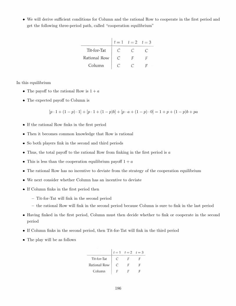
� We will derive sufficient conditions for Column and the rational Row to cooperate in the first period and
get the following three-period path, called “cooperation equilibrium”
In this equilibrium
� The payoff to the rational Row is 1 + a
� The expected payoff to Column is
[p · 1 + (1− p) · 1] + [p · 1 + (1− p)b] + [p · a+ (1− p) · 0] = 1 + p+ (1− p)b+ pa
� If the rational Row finks in the first period
� Then it becomes common knowledge that Row is rational
� So both players fink in the second and third periods
� Thus, the total payoff to the rational Row from finking in the first period is a
� This is less than the cooperation equilibrium payoff 1 + a
� The rational Row has no incentive to deviate from the strategy of the cooperation equilibrium
� We next consider whether Column has an incentive to deviate
� If Column finks in the first period then
– Tit-for-Tat will fink in the second period
– the rational Row will fink in the second period because Column is sure to fink in the last period
� Having finked in the first period, Column must then decide whether to fink or cooperate in the second
period
� If Column finks in the second period, then Tit-for-Tat will fink in the third period
� The play will be as follows
186
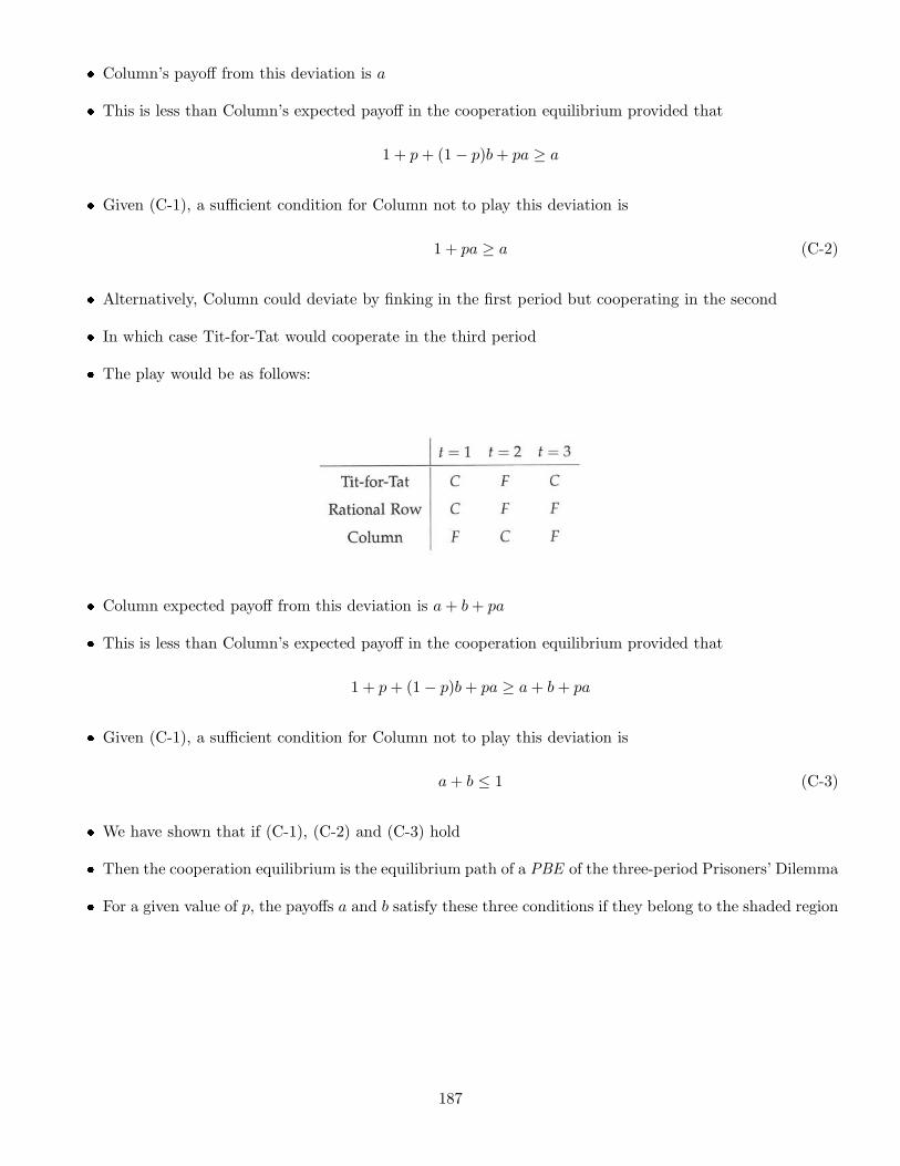
� Column’s payoff from this deviation is a
� This is less than Column’s expected payoff in the cooperation equilibrium provided that
1 + p+ (1− p)b+ pa ≥ a
� Given (C-1), a sufficient condition for Column not to play this deviation is
1 + pa ≥ a (C-2)
� Alternatively, Column could deviate by finking in the first period but cooperating in the second
� In which case Tit-for-Tat would cooperate in the third period
� The play would be as follows:
� Column expected payoff from this deviation is a+ b+ pa
� This is less than Column’s expected payoff in the cooperation equilibrium provided that
1 + p+ (1− p)b+ pa ≥ a+ b+ pa
� Given (C-1), a sufficient condition for Column not to play this deviation is
a+ b ≤ 1 (C-3)
� We have shown that if (C-1), (C-2) and (C-3) hold
� Then the cooperation equilibrium is the equilibrium path of a PBE of the three-period Prisoners’ Dilemma
� For a given value of p, the payoffs a and b satisfy these three conditions if they belong to the shaded region
187
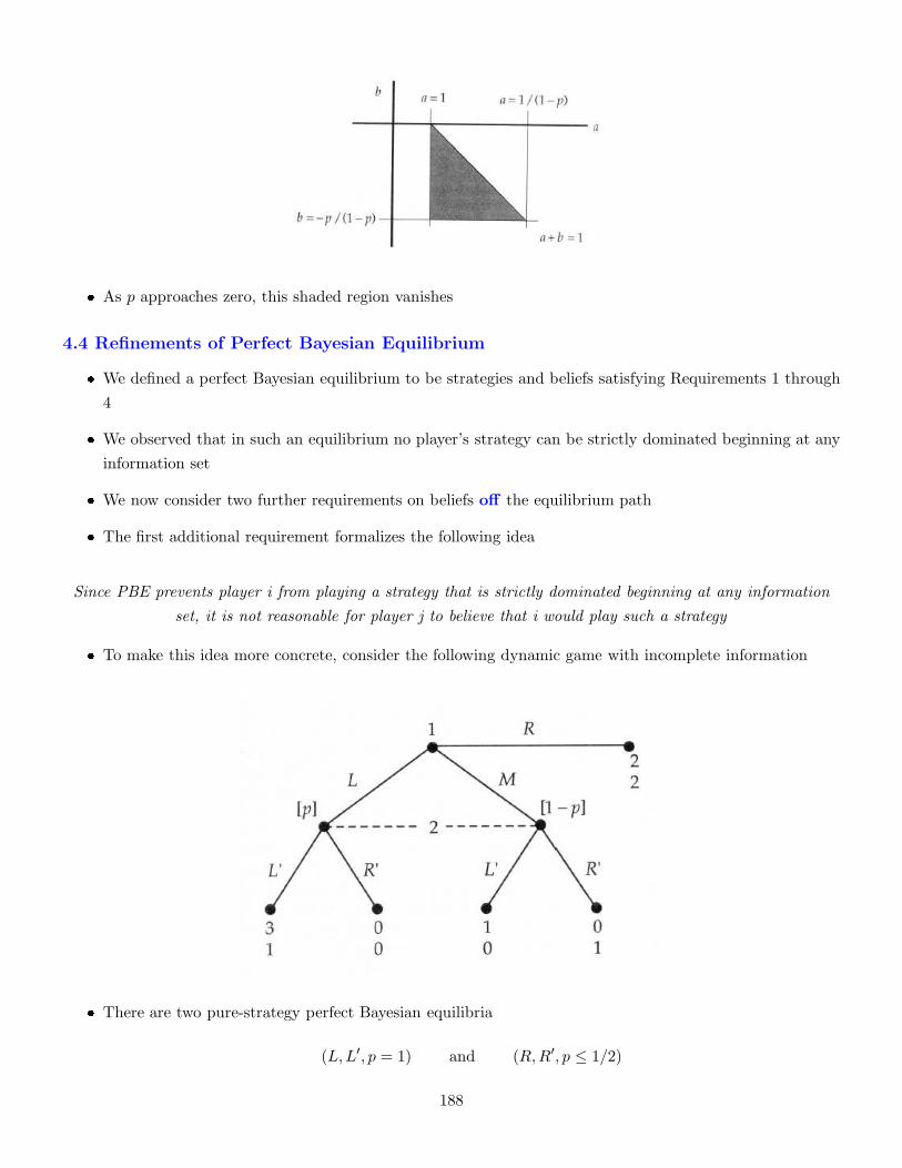
� As p approaches zero, this shaded region vanishes
4.4 Refinements of Perfect Bayesian Equilibrium
� We defined a perfect Bayesian equilibrium to be strategies and beliefs satisfying Requirements 1 through
4
� We observed that in such an equilibrium no player’s strategy can be strictly dominated beginning at any
information set
� We now consider two further requirements on beliefs off the equilibrium path
� The first additional requirement formalizes the following idea
Since PBE prevents player i from playing a strategy that is strictly dominated beginning at any information
set, it is not reasonable for player j to believe that i would play such a strategy
� To make this idea more concrete, consider the following dynamic game with incomplete information
� There are two pure-strategy perfect Bayesian equilibria
(L,L′, p = 1) and (R,R′, p ≤ 1/2)
188
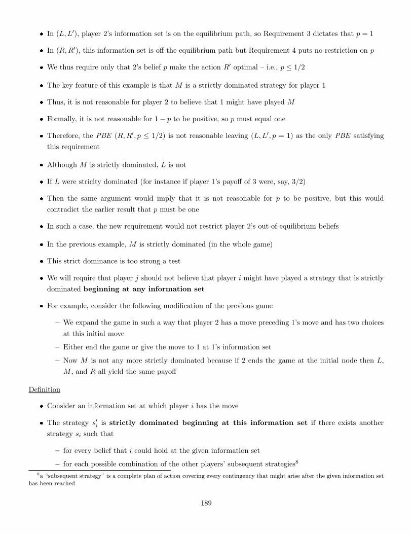
� In (L,L′), player 2’s information set is on the equilibrium path, so Requirement 3 dictates that p = 1
� In (R,R′), this information set is off the equilibrium path but Requirement 4 puts no restriction on p
� We thus require only that 2’s belief p make the action R′ optimal – i.e., p ≤ 1/2
� The key feature of this example is that M is a strictly dominated strategy for player 1
� Thus, it is not reasonable for player 2 to believe that 1 might have played M
� Formally, it is not reasonable for 1− p to be positive, so p must equal one
� Therefore, the PBE (R,R′, p ≤ 1/2) is not reasonable leaving (L,L′, p = 1) as the only PBE satisfying
this requirement
� Although M is strictly dominated, L is not
� If L were striclty dominated (for instance if player 1’s payoff of 3 were, say, 3/2)
� Then the same argument would imply that it is not reasonable for p to be positive, but this would
contradict the earlier result that p must be one
� In such a case, the new requirement would not restrict player 2’s out-of-equilibrium beliefs
� In the previous example, M is strictly dominated (in the whole game)
� This strict dominance is too strong a test
� We will require that player j should not believe that player i might have played a strategy that is strictly
dominated beginning at any information set
� For example, consider the following modification of the previous game
– We expand the game in such a way that player 2 has a move preceding 1’s move and has two choices
at this initial move
– Either end the game or give the move to 1 at 1’s information set
– Now M is not any more strictly dominated because if 2 ends the game at the initial node then L,
M , and R all yield the same payoff
Definition
� Consider an information set at which player i has the move
� The strategy s′i is strictly dominated beginning at this information set if there exists another
strategy si such that
– for every belief that i could hold at the given information set
– for each possible combination of the other players’ subsequent strategies8
8a “subsequent strategy” is a complete plan of action covering every contingency that might arise after the given information sethas been reached
189
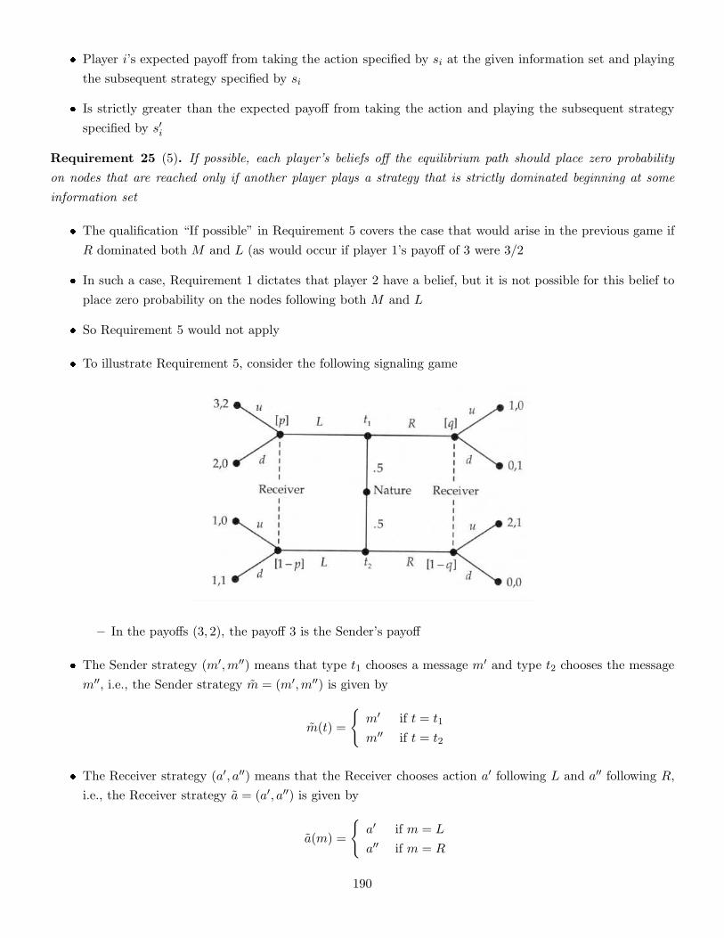
� Player i’s expected payoff from taking the action specified by si at the given information set and playing
the subsequent strategy specified by si
� Is strictly greater than the expected payoff from taking the action and playing the subsequent strategy
specified by s′i
Requirement 25 (5). If possible, each player’s beliefs off the equilibrium path should place zero probability
on nodes that are reached only if another player plays a strategy that is strictly dominated beginning at some
information set
� The qualification “If possible” in Requirement 5 covers the case that would arise in the previous game if
R dominated both M and L (as would occur if player 1’s payoff of 3 were 3/2
� In such a case, Requirement 1 dictates that player 2 have a belief, but it is not possible for this belief to
place zero probability on the nodes following both M and L
� So Requirement 5 would not apply
� To illustrate Requirement 5, consider the following signaling game
– In the payoffs (3, 2), the payoff 3 is the Sender’s payoff
� The Sender strategy (m′,m′′) means that type t1 chooses a message m′ and type t2 chooses the message
m′′, i.e., the Sender strategy m = (m′,m′′) is given by
m(t) =
{
m′ if t = t1
m′′ if t = t2
� The Receiver strategy (a′, a′′) means that the Receiver chooses action a′ following L and a′′ following R,
i.e., the Receiver strategy a = (a′, a′′) is given by
a(m) =
{
a′ if m = L
a′′ if m = R
190
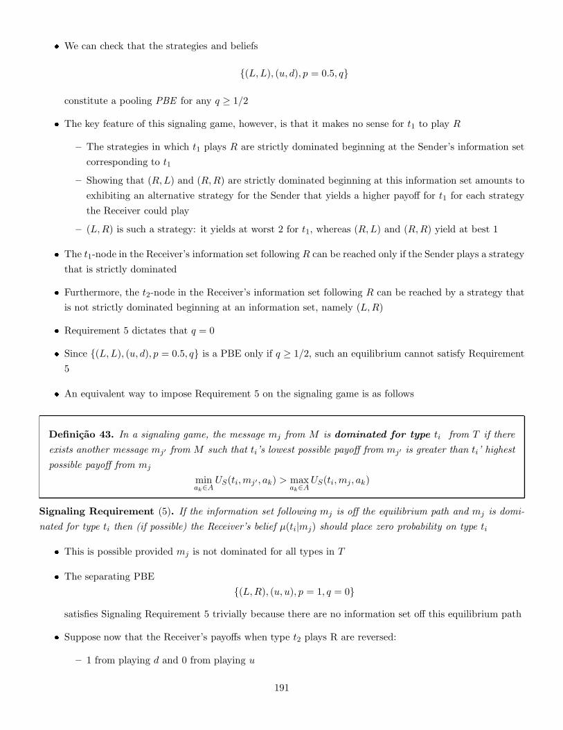
� We can check that the strategies and beliefs
{(L,L), (u, d), p = 0.5, q}
constitute a pooling PBE for any q ≥ 1/2
� The key feature of this signaling game, however, is that it makes no sense for t1 to play R
– The strategies in which t1 plays R are strictly dominated beginning at the Sender’s information set
corresponding to t1
– Showing that (R,L) and (R,R) are strictly dominated beginning at this information set amounts to
exhibiting an alternative strategy for the Sender that yields a higher payoff for t1 for each strategy
the Receiver could play
– (L,R) is such a strategy: it yields at worst 2 for t1, whereas (R,L) and (R,R) yield at best 1
� The t1-node in the Receiver’s information set following R can be reached only if the Sender plays a strategy
that is strictly dominated
� Furthermore, the t2-node in the Receiver’s information set following R can be reached by a strategy that
is not strictly dominated beginning at an information set, namely (L,R)
� Requirement 5 dictates that q = 0
� Since {(L,L), (u, d), p = 0.5, q} is a PBE only if q ≥ 1/2, such an equilibrium cannot satisfy Requirement
5
� An equivalent way to impose Requirement 5 on the signaling game is as follows
Definicao 43. In a signaling game, the message mj from M is dominated for type ti from T if there
exists another message mj′ from M such that ti’s lowest possible payoff from mj′ is greater than ti’ highest
possible payoff from mj
minak∈A
US(ti,mj′ , ak) > maxak∈A
US(ti,mj, ak)
Signaling Requirement (5). If the information set following mj is off the equilibrium path and mj is domi-
nated for type ti then (if possible) the Receiver’s belief µ(ti|mj) should place zero probability on type ti
� This is possible provided mj is not dominated for all types in T
� The separating PBE
{(L,R), (u, u), p = 1, q = 0}
satisfies Signaling Requirement 5 trivially because there are no information set off this equilibrium path
� Suppose now that the Receiver’s payoffs when type t2 plays R are reversed:
– 1 from playing d and 0 from playing u
191
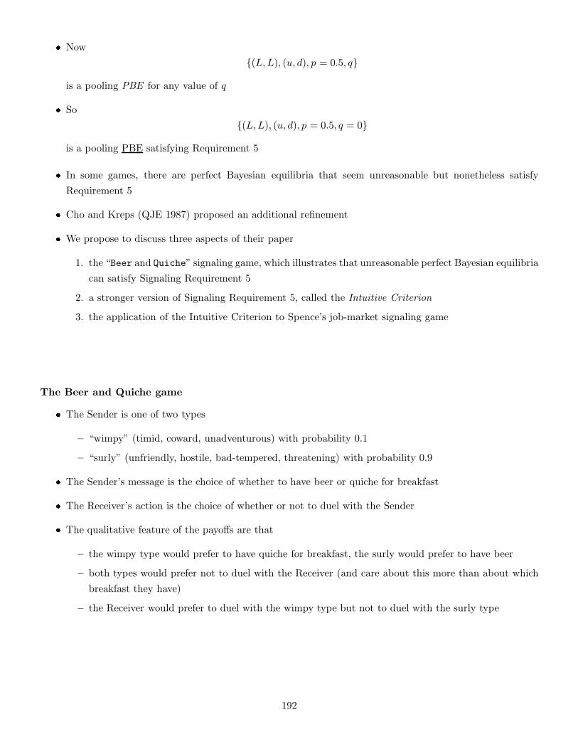
� Now
{(L,L), (u, d), p = 0.5, q}
is a pooling PBE for any value of q
� So
{(L,L), (u, d), p = 0.5, q = 0}
is a pooling PBE satisfying Requirement 5
� In some games, there are perfect Bayesian equilibria that seem unreasonable but nonetheless satisfy
Requirement 5
� Cho and Kreps (QJE 1987) proposed an additional refinement
� We propose to discuss three aspects of their paper
1. the “Beer and Quiche” signaling game, which illustrates that unreasonable perfect Bayesian equilibria
can satisfy Signaling Requirement 5
2. a stronger version of Signaling Requirement 5, called the Intuitive Criterion
3. the application of the Intuitive Criterion to Spence’s job-market signaling game
The Beer and Quiche game
� The Sender is one of two types
– “wimpy” (timid, coward, unadventurous) with probability 0.1
– “surly” (unfriendly, hostile, bad-tempered, threatening) with probability 0.9
� The Sender’s message is the choice of whether to have beer or quiche for breakfast
� The Receiver’s action is the choice of whether or not to duel with the Sender
� The qualitative feature of the payoffs are that
– the wimpy type would prefer to have quiche for breakfast, the surly would prefer to have beer
– both types would prefer not to duel with the Receiver (and care about this more than about which
breakfast they have)
– the Receiver would prefer to duel with the wimpy type but not to duel with the surly type
192
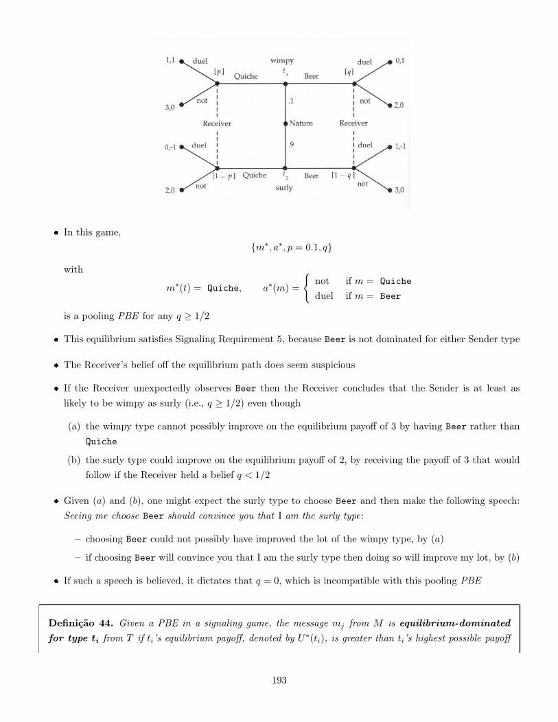
� In this game,
{m∗, a∗, p = 0.1, q}
with
m∗(t) = Quiche, a∗(m) =
{
not if m = Quiche
duel if m = Beer
is a pooling PBE for any q ≥ 1/2
� This equilibrium satisfies Signaling Requirement 5, because Beer is not dominated for either Sender type
� The Receiver’s belief off the equilibrium path does seem suspicious
� If the Receiver unexpectedly observes Beer then the Receiver concludes that the Sender is at least as
likely to be wimpy as surly (i.e., q ≥ 1/2) even though
(a) the wimpy type cannot possibly improve on the equilibrium payoff of 3 by having Beer rather than
Quiche
(b) the surly type could improve on the equilibrium payoff of 2, by receiving the payoff of 3 that would
follow if the Receiver held a belief q < 1/2
� Given (a) and (b), one might expect the surly type to choose Beer and then make the following speech:
Seeing me choose Beer should convince you that I am the surly type:
– choosing Beer could not possibly have improved the lot of the wimpy type, by (a)
– if choosing Beer will convince you that I am the surly type then doing so will improve my lot, by (b)
� If such a speech is believed, it dictates that q = 0, which is incompatible with this pooling PBE
Definicao 44. Given a PBE in a signaling game, the message mj from M is equilibrium-dominated
for type ti from T if ti’s equilibrium payoff, denoted by U∗(ti), is greater than ti’s highest possible payoff
193
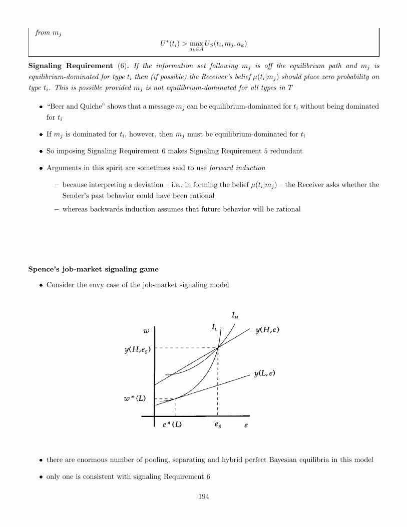
from mj
U∗(ti) > maxak∈A
US(ti,mj , ak)
Signaling Requirement (6). If the information set following mj is off the equilibrium path and mj is
equilibrium-dominated for type ti then (if possible) the Receiver’s belief µ(ti|mj) should place zero probability on
type ti. This is possible provided mj is not equilibrium-dominated for all types in T
� “Beer and Quiche” shows that a message mj can be equilibrium-dominated for ti without being dominated
for ti
� If mj is dominated for ti, however, then mj must be equilibrium-dominated for ti
� So imposing Signaling Requirement 6 makes Signaling Requirement 5 redundant
� Arguments in this spirit are sometimes said to use forward induction
– because interpreting a deviation – i.e., in forming the belief µ(ti|mj) – the Receiver asks whether the
Sender’s past behavior could have been rational
– whereas backwards induction assumes that future behavior will be rational
Spence’s job-market signaling game
� Consider the envy case of the job-market signaling model
� there are enormous number of pooling, separating and hybrid perfect Bayesian equilibria in this model
� only one is consistent with signaling Requirement 6
194
– ti = L chooses e∗(L)
– ti = H chooses es
� Remember that, in any PBE, worker’s wage is
w(e) = µ(H|e) · y(H, e) + (1− µ(H|e)) · y(L, e)
� Because
y[L, e∗(L)]− c[L, e∗(L)] > w(e) − c(L, e) ∀e > es
any education level e > es is dominated for the low-ability type
– in terms of Signaling Requirement 5
– therefore, µ(H|e) = 1 for all e > es
� There is no other separating PBE satisfying Signaling Requirement 5
� For any PBE with e(H) = e, e > es, a deviation would be choose e ∈ [es, e)
– see the previous figure
� in any equilibrium that satisfies Signaling Requirement 5, type-H’s utility must be at least
y(H, es)− c(H, es)
otherwise, the worker would deviate to (w, e) = (y(H, es), es)
� Some pooling and hybrid equilibria cannot satisfy Signaling Requirement 5
� There are 2 cases:
(a) q is low enough
(b) q is not low enough
that the wage function
w = q · y(H, e) + (1− q) · y(L, e)
is below the high-ability worker’s indifference curve through the point [es, y(H, es)]
� First, consider case (a):
195
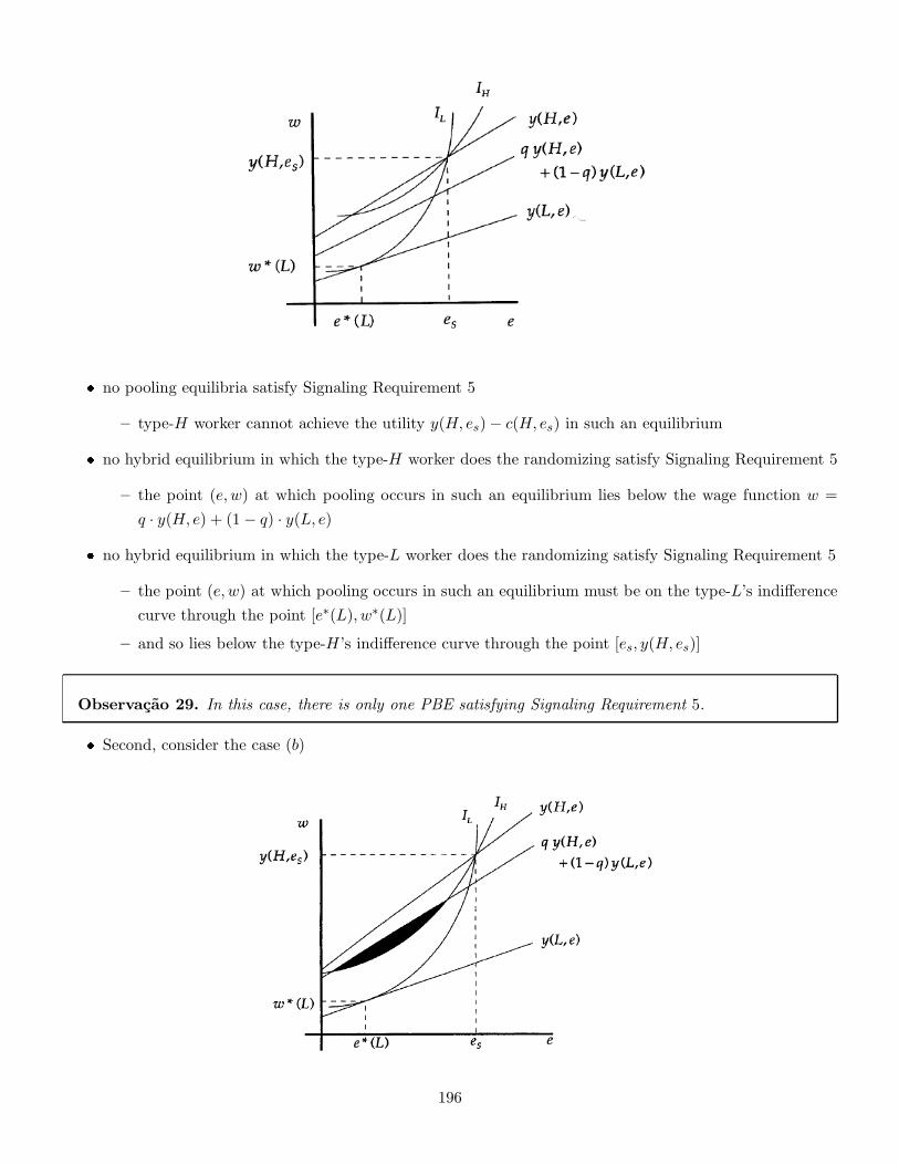
� no pooling equilibria satisfy Signaling Requirement 5
– type-H worker cannot achieve the utility y(H, es)− c(H, es) in such an equilibrium
� no hybrid equilibrium in which the type-H worker does the randomizing satisfy Signaling Requirement 5
– the point (e, w) at which pooling occurs in such an equilibrium lies below the wage function w =
q · y(H, e) + (1− q) · y(L, e)
� no hybrid equilibrium in which the type-L worker does the randomizing satisfy Signaling Requirement 5
– the point (e, w) at which pooling occurs in such an equilibrium must be on the type-L’s indifference
curve through the point [e∗(L), w∗(L)]
– and so lies below the type-H’s indifference curve through the point [es, y(H, es)]
Observacao 29. In this case, there is only one PBE satisfying Signaling Requirement 5.
� Second, consider the case (b)
196
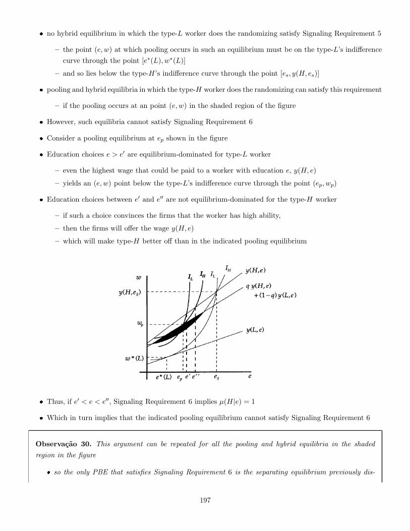
� no hybrid equilibrium in which the type-L worker does the randomizing satisfy Signaling Requirement 5
– the point (e, w) at which pooling occurs in such an equilibrium must be on the type-L’s indifference
curve through the point [e∗(L), w∗(L)]
– and so lies below the type-H’s indifference curve through the point [es, y(H, es)]
� pooling and hybrid equilibria in which the type-H worker does the randomizing can satisfy this requirement
– if the pooling occurs at an point (e, w) in the shaded region of the figure
� However, such equilibria cannot satisfy Signaling Requirement 6
� Consider a pooling equilibrium at ep shown in the figure
� Education choices e > e′ are equilibrium-dominated for type-L worker
– even the highest wage that could be paid to a worker with education e, y(H, e)
– yields an (e, w) point below the type-L’s indifference curve through the point (ep, wp)
� Education choices between e′ and e′′ are not equilibrium-dominated for the type-H worker
– if such a choice convinces the firms that the worker has high ability,
– then the firms will offer the wage y(H, e)
– which will make type-H better off than in the indicated pooling equilibrium
� Thus, if e′ < e < e′′, Signaling Requirement 6 implies µ(H|e) = 1
� Which in turn implies that the indicated pooling equilibrium cannot satisfy Signaling Requirement 6
Observacao 30. This argument can be repeated for all the pooling and hybrid equilibria in the shaded
region in the figure
� so the only PBE that satisfies Signaling Requirement 6 is the separating equilibrium previously dis-
197

cussed
198
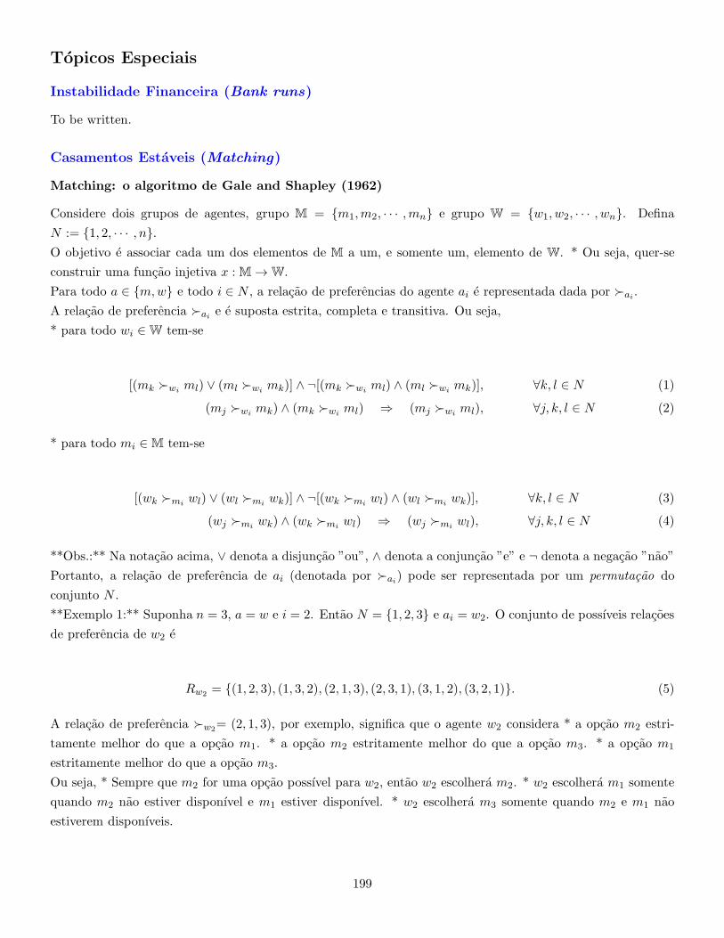
Topicos Especiais
Instabilidade Financeira (Bank runs)
To be written.
Casamentos Estaveis (Matching)
Matching: o algoritmo de Gale and Shapley (1962)
Considere dois grupos de agentes, grupo M = {m1,m2, · · · ,mn} e grupo W = {w1, w2, · · · , wn}. Defina
N := {1, 2, · · · , n}.O objetivo e associar cada um dos elementos de M a um, e somente um, elemento de W. * Ou seja, quer-se
construir uma funcao injetiva x : M → W.
Para todo a ∈ {m,w} e todo i ∈ N , a relacao de preferencias do agente ai e representada dada por ≻ai .
A relacao de preferencia ≻ai e e suposta estrita, completa e transitiva. Ou seja,
* para todo wi ∈ W tem-se
[(mk ≻wiml) ∨ (ml ≻wi
mk)] ∧ ¬[(mk ≻wiml) ∧ (ml ≻wi
mk)], ∀k, l ∈ N (1)
(mj ≻wimk) ∧ (mk ≻wi
ml) ⇒ (mj ≻wiml), ∀j, k, l ∈ N (2)
* para todo mi ∈ M tem-se
[(wk ≻miwl) ∨ (wl ≻mi
wk)] ∧ ¬[(wk ≻miwl) ∧ (wl ≻mi
wk)], ∀k, l ∈ N (3)
(wj ≻miwk) ∧ (wk ≻mi
wl) ⇒ (wj ≻miwl), ∀j, k, l ∈ N (4)
**Obs.:** Na notacao acima, ∨ denota a disjuncao ”ou”, ∧ denota a conjuncao ”e” e ¬ denota a negacao ”nao”
Portanto, a relacao de preferencia de ai (denotada por ≻ai) pode ser representada por um permutacao do
conjunto N .
**Exemplo 1:** Suponha n = 3, a = w e i = 2. Entao N = {1, 2, 3} e ai = w2. O conjunto de possıveis relacoes
de preferencia de w2 e
Rw2= {(1, 2, 3), (1, 3, 2), (2, 1, 3), (2, 3, 1), (3, 1, 2), (3, 2, 1)}. (5)
A relacao de preferencia ≻w2= (2, 1, 3), por exemplo, significa que o agente w2 considera * a opcao m2 estri-
tamente melhor do que a opcao m1. * a opcao m2 estritamente melhor do que a opcao m3. * a opcao m1
estritamente melhor do que a opcao m3.
Ou seja, * Sempre que m2 for uma opcao possıvel para w2, entao w2 escolhera m2. * w2 escolhera m1 somente
quando m2 nao estiver disponıvel e m1 estiver disponıvel. * w2 escolhera m3 somente quando m2 e m1 nao
estiverem disponıveis.
199
**Exemplo 2 (descricao completa em [ams.org](http://www.ams.org/samplings/feature-column/fc-2015-03)):**
Suponha N = 4 e que as relacoes de preferencia de mi e de wi sao representadas pela i-esima linha da matriz
M e W , respectivamente.
M =
w1 w2 w3 w4
w1 w4 w3 w2
w2 w1 w3 w4
w4 w2 w3 w1
, W =
m4 m3 m1 m2
m2 m4 m1 m3
m4 m1 m2 m3
m3 m2 m1 m4
(6)
Por exemplo, a preferencia de m3 e dada por ≻m3= (2, 1, 3, 4).
O algoritmo:
O objetivo do algoritmo e computar a funcao injetiva x : M → W. Tal funcao e calculada como o limite de
uma sequencia de funcoes {xt}Tt=0 tal que xt : M → W para todo t. O valor de T e escolhido de forma que
xT = xT−1. Ele segue os passos a seguir:
Passo 0: O primeiro elemento da sequencia, x0 e escolhido neste passo. Cada m ∈ M e associado ao elemento
de W mais peferido por m, ou seja,
x0(m) = min{≻(i)m : wi ∈ W}, ∀m ∈ M. (7)
em que ≻(i)m denota a i-esima entrada de ≻m.
� Passo 0.1: Considere um elemento w ∈ W arbitrario. O conjunto de elementos de M associados a w via
x0 e dado por
M0w = {m ∈ M : x0(m) = w} ⊆ M. (8)
Deste conjunto, w escolhe seu elemento preferido, min{≻(i)w : mi ∈ M0
w}, e rejeita os demais.
� Passo 0.2: Considere um elemento m ∈ M arbitrario. O conjunto de elementos de W que nao rejeitaram
m e dado por
W 0m = W \ {w ∈ W : (x0(m) = w) ∧ (m 6= min{≻(i)
w : mi ∈ M0w})} ⊆ W. (9)
�
Passo k > 0: Cada m ∈ M e associado ao elemento de W k−1m mais peferido por m, ou seja,
xk(m) = min{≻(i)m : wi ∈ W k−1
m }, ∀m ∈ M. (10)
� Passo k.1: Considere um elemento w ∈ W arbitrario. O conjunto de elementos de M associados a w via
xk e dado por
Mkw = {m ∈ M : xk(m) = w} ⊆ M.
200
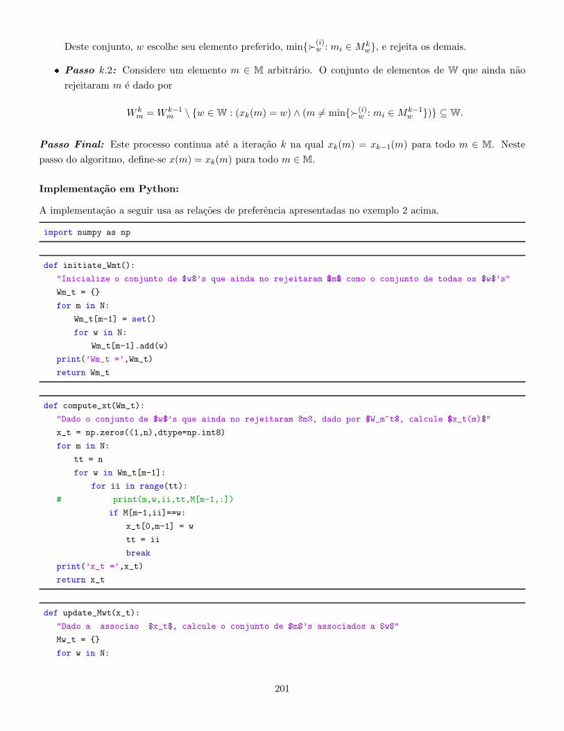
Deste conjunto, w escolhe seu elemento preferido, min{≻(i)w : mi ∈ Mk
w}, e rejeita os demais.
� Passo k.2: Considere um elemento m ∈ M arbitrario. O conjunto de elementos de W que ainda nao
rejeitaram m e dado por
W km = W k−1
m \ {w ∈ W : (xk(m) = w) ∧ (m 6= min{≻(i)w : mi ∈ Mk−1
w })} ⊆ W.
Passo Final: Este processo continua ate a iteracao k na qual xk(m) = xk−1(m) para todo m ∈ M. Neste
passo do algoritmo, define-se x(m) = xk(m) para todo m ∈ M.
Implementacao em Python:
A implementacao a seguir usa as relacoes de preferencia apresentadas no exemplo 2 acima.
import numpy as np
def initiate_Wmt():
"Inicialize o conjunto de $w$’s que ainda no rejeitaram $m$ como o conjunto de todas os $w$’s"
Wm_t = {}
for m in N:
Wm_t[m-1] = set()
for w in N:
Wm_t[m-1].add(w)
print(’Wm_t =’,Wm_t)
return Wm_t
def compute_xt(Wm_t):
"Dado o conjunto de $w$’s que ainda no rejeitaram $m$, dado por $W_m^t$, calcule $x_t(m)$"
x_t = np.zeros((1,n),dtype=np.int8)
for m in N:
tt = n
for w in Wm_t[m-1]:
for ii in range(tt):
# print(m,w,ii,tt,M[m-1,:])
if M[m-1,ii]==w:
x_t[0,m-1] = w
tt = ii
break
print(’x_t =’,x_t)
return x_t
def update_Mwt(x_t):
"Dado a associao $x_t$, calcule o conjunto de $m$’s associados a $w$"
Mw_t = {}
for w in N:
201
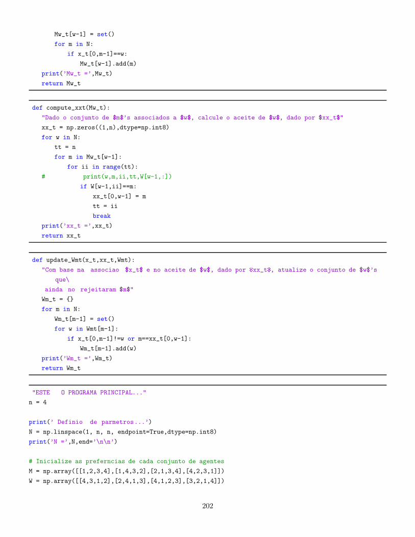
Mw_t[w-1] = set()
for m in N:
if x_t[0,m-1]==w:
Mw_t[w-1].add(m)
print(’Mw_t =’,Mw_t)
return Mw_t
def compute_xxt(Mw_t):
"Dado o conjunto de $m$’s associados a $w$, calcule o aceite de $w$, dado por $xx_t$"
xx_t = np.zeros((1,n),dtype=np.int8)
for w in N:
tt = n
for m in Mw_t[w-1]:
for ii in range(tt):
# print(w,m,ii,tt,W[w-1,:])
if W[w-1,ii]==m:
xx_t[0,w-1] = m
tt = ii
break
print(’xx_t =’,xx_t)
return xx_t
def update_Wmt(x_t,xx_t,Wmt):
"Com base na associao $x_t$ e no aceite de $w$, dado por $xx_t$, atualize o conjunto de $w$’s
que\
ainda no rejeitaram $m$"
Wm_t = {}
for m in N:
Wm_t[m-1] = set()
for w in Wmt[m-1]:
if x_t[0,m-1]!=w or m==xx_t[0,w-1]:
Wm_t[m-1].add(w)
print(’Wm_t =’,Wm_t)
return Wm_t
"ESTE O PROGRAMA PRINCIPAL..."
n = 4
print(’ Definio de parmetros...’)
N = np.linspace(1, n, n, endpoint=True,dtype=np.int8)
print(’N =’,N,end=’\n\n’)
# Inicialize as preferncias de cada conjunto de agentes
M = np.array([[1,2,3,4],[1,4,3,2],[2,1,3,4],[4,2,3,1]])
W = np.array([[4,3,1,2],[2,4,1,3],[4,1,2,3],[3,2,1,4]])
202
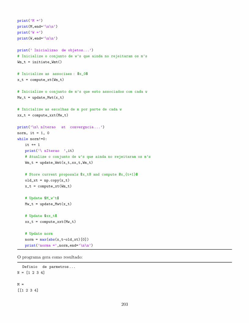
print(’M =’)
print(M,end=’\n\n’)
print(’W =’)
print(W,end=’\n\n’)
print(’ Inicializao de objetos...’)
# Inicialize o conjunto de w’s que ainda no rejeitaram os m’s
Wm_t = initiate_Wmt()
# Inicialize as associaes : $x_0$
x_t = compute_xt(Wm_t)
# Inicialize o conjunto de m’s que esto associados com cada w
Mw_t = update_Mwt(x_t)
# Inicialize as escolhas de m por parte de cada w
xx_t = compute_xxt(Mw_t)
print(’\n\ nIterao at convergncia...’)
norm, it = 1, 0
while norm!=0:
it += 1
print(’\ nIterao ’,it)
# Atualize o conjunto de w’s que ainda no rejeitaram os m’s
Wm_t = update_Wmt(x_t,xx_t,Wm_t)
# Store current proposals $x_t$ and compute $x_{t+1}$
old_xt = np.copy(x_t)
x_t = compute_xt(Wm_t)
# Update $M_w^t$
Mw_t = update_Mwt(x_t)
# Update $xx_t$
xx_t = compute_xxt(Mw_t)
# Update norm
norm = max(abs(x_t-old_xt)[0])
print(’norma =’,norm,end=’\n\n’)
O programa gera como resultado:
Definio de parmetros...
N = [1 2 3 4]
M =
[[1 2 3 4]
203
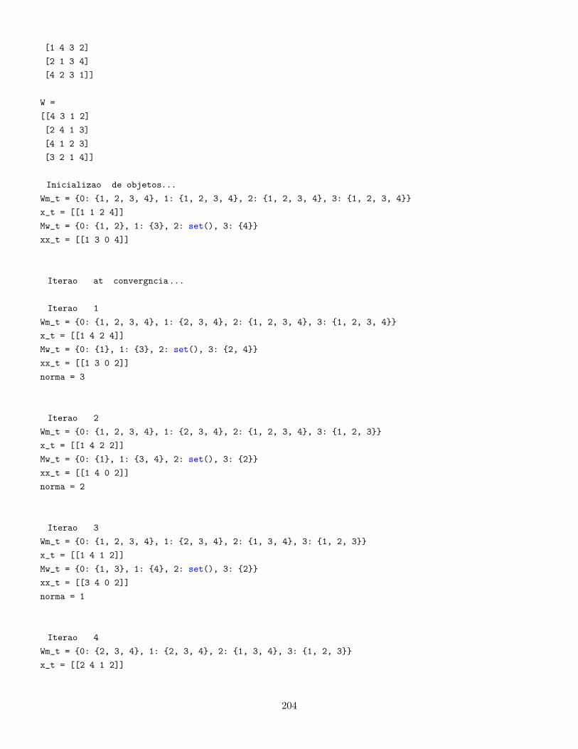
[1 4 3 2]
[2 1 3 4]
[4 2 3 1]]
W =
[[4 3 1 2]
[2 4 1 3]
[4 1 2 3]
[3 2 1 4]]
Inicializao de objetos...
Wm_t = {0: {1, 2, 3, 4}, 1: {1, 2, 3, 4}, 2: {1, 2, 3, 4}, 3: {1, 2, 3, 4}}
x_t = [[1 1 2 4]]
Mw_t = {0: {1, 2}, 1: {3}, 2: set(), 3: {4}}
xx_t = [[1 3 0 4]]
Iterao at convergncia...
Iterao 1
Wm_t = {0: {1, 2, 3, 4}, 1: {2, 3, 4}, 2: {1, 2, 3, 4}, 3: {1, 2, 3, 4}}
x_t = [[1 4 2 4]]
Mw_t = {0: {1}, 1: {3}, 2: set(), 3: {2, 4}}
xx_t = [[1 3 0 2]]
norma = 3
Iterao 2
Wm_t = {0: {1, 2, 3, 4}, 1: {2, 3, 4}, 2: {1, 2, 3, 4}, 3: {1, 2, 3}}
x_t = [[1 4 2 2]]
Mw_t = {0: {1}, 1: {3, 4}, 2: set(), 3: {2}}
xx_t = [[1 4 0 2]]
norma = 2
Iterao 3
Wm_t = {0: {1, 2, 3, 4}, 1: {2, 3, 4}, 2: {1, 3, 4}, 3: {1, 2, 3}}
x_t = [[1 4 1 2]]
Mw_t = {0: {1, 3}, 1: {4}, 2: set(), 3: {2}}
xx_t = [[3 4 0 2]]
norma = 1
Iterao 4
Wm_t = {0: {2, 3, 4}, 1: {2, 3, 4}, 2: {1, 3, 4}, 3: {1, 2, 3}}
x_t = [[2 4 1 2]]
204
Mw_t = {0: {3}, 1: {1, 4}, 2: set(), 3: {2}}
xx_t = [[3 4 0 2]]
norma = 1
Iterao 5
Wm_t = {0: {3, 4}, 1: {2, 3, 4}, 2: {1, 3, 4}, 3: {1, 2, 3}}
x_t = [[3 4 1 2]]
Mw_t = {0: {3}, 1: {4}, 2: {1}, 3: {2}}
xx_t = [[3 4 1 2]]
norma = 1
Iterao 6
Wm_t = {0: {3, 4}, 1: {2, 3, 4}, 2: {1, 3, 4}, 3: {1, 2, 3}}
x_t = [[3 4 1 2]]
Mw_t = {0: {3}, 1: {4}, 2: {1}, 3: {2}}
xx_t = [[3 4 1 2]]
norma = 0
References
J. Bertrand. Review of recherches sur le principe mathematique de latheorie des richesses. Journal des Savants,
499, 1883.
I.-K. Cho and D. M. Kreps. Signaling games and stable equilibria. The Quarterly Journal of Economics, 102
(2):179–221, 1987.
A.-A. Cournot. Recherches sur les principes mathematiques de la theorie des richesses par Augustin Cournot.
chez L. Hachette, 1838.
D. W. Diamond and P. H. Dybvig. Bank runs, deposit insurance, and liquidity. Journal of political economy,
91(3):401–419, 1983.
M. P. Espinosa and C. Rhee. Efficient wage bargaining as a repeated game. The Quarterly Journal of Economics,
104(3):565–588, 1989.
J. W. Friedman. A non-cooperative equilibrium for supergames. The Review of Economic Studies, 38(1):1–12,
1971.
D. Gale and L. S. Shapley. College admissions and the stability of marriage. The American Mathematical
Monthly, 69(1):9–15, 1962.
R. Gibbons. Game Theory for Applied Economists. Princeton University Press, 1992. ISBN 9781400835881.
J. C. Harsanyi. Games with incomplete information played by” bayesian” players, i-iii. part ii. bayesian equi-
librium points. Management Science, pages 320–334, 1968.
205
J. C. Harsanyi. Games with randomly disturbed payoffs: A new rationale for mixed-strategy equilibrium points.
International Journal of Game Theory, 2(1):1–23, 1973.
E. P. Lazear and S. Rosen. Rank-order tournaments as optimum labor contracts. Journal of political Economy,
89(5):841–864, 1981.
W. Leontief. The pure theory of the guaranteed annual wage contract. Journal of Political Economy, 54(1):
76–79, 1946.
J. F. Nash et al. Equilibrium points in n-person games. Proceedings of the national academy of sciences, 36(1):
48–49, 1950.
H. Von Stackelberg. Marktform und gleichgewicht. J. springer, 1934.
206