Notes on Dynamic ProgrammingAlgorithms & Data Structures

Dr Mary Cryan

These notes are to accompany lectures 10 and 11 of ADS.

1 Introduction

The technique of Dynamic Programming (DP) could be described “recursion turned upside-down”.However, it is not usually used as an alternative to recursion. Rather, dynamic programmingis used (if possible) for cases when a recurrence for an algorithmic problem will not run inpolynomial-time if it is implemented recursively. So in fact Dynamic Programming is a more-powerful technique than basic Divide-and-Conquer.

Designing, Analysing and Implementing a dynamic programming algorithm is (like Divide-and-Conquer) highly problem specific. However, there are particular features shared by mostdynamic programming algorithms, and we describe them below on page 2 (dp1(a), dp1(b), dp2,dp3). It will be helpful to carry along an introductory example-problem to illustrate these fea-tures. The introductory problem will be the problem of computing the nth Fibonacci number,where F(n) is defined as follows:

F0 = 0,

F1 = 1,

Fn = Fn−1 + Fn−2 (for n ≥ 2).

Since Fibonacci numbers are defined recursively, the definition suggests a very natural recursivealgorithm to compute F(n):

Algorithm REC-FIB(n)

1. if n = 0 then

2. return 0

3. else if n = 1 then

4. return 1

5. else

6. return REC-FIB(n− 1) + REC-FIB(n− 2)

First note that were we to implement REC-FIB, we would not be able to use the Master Theo-rem to analyse its running-time. The recurrence for the running-time TREC-FIB(n) that we wouldget would be

TREC-FIB(n) = TREC-FIB(n− 1) + TREC-FIB(n− 2) +Θ(1), (1)

where the Θ(1) comes from the fact that, at most, we have to do enough work to add two valuestogether (on line 6). The Master Theorem cannot be used to analyse this recurrence because therecursive calls have sizes n−1 and n−2, rather than size n/b for some b > 1. The actual presenceof non-b/n calls need not *necessarily* exclude the possibility of proving a good running-time -for example, if we think back to QUICKSORT (lecture 8), the worst-case recurrence for QUICKSORT

contains a call of size n − 1. However, the particular form of (1) does in fact imply that TREC-FIB(n)is exponential - by examining (1) and noting its similarity with the recurrence defining F(n), wefind TREC-FIB(n) ≥ F(n). But Fn ≈ 1.6n as n gets large. We won’t prove this lower bound, but seeour BOARD NOTE for a proof that F(n) ≥ 1

2(3/2)n for n ≥ 8.

1

Notes on Dynamic Programming ADS

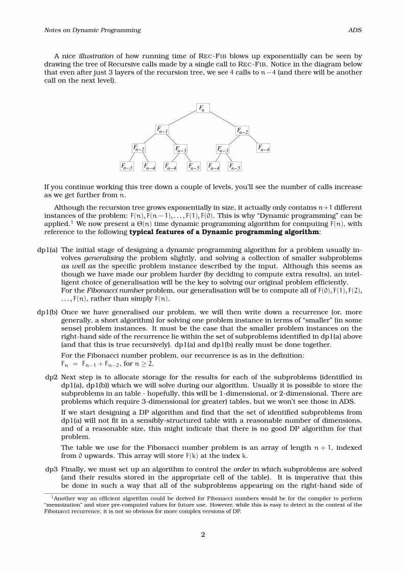
A nice illustration of how running time of REC-FIB blows up exponentially can be seen bydrawing the tree of Recursive calls made by a single call to REC-FIB. Notice in the diagram belowthat even after just 3 layers of the recursion tree, we see 4 calls to n−4 (and there will be anothercall on the next level).

Fn

Fn−1 Fn−2

Fn−3 Fn−4Fn−2 Fn−3

Fn−4 Fn−4 Fn−5 Fn−4 Fn−5Fn−3

If you continue working this tree down a couple of levels, you’ll see the number of calls increaseas we get further from n.

Although the recursion tree grows exponentially in size, it actually only contains n+1 differentinstances of the problem: F(n), F(n− 1), . . . , F(1), F(0). This is why “Dynamic programming” can beapplied.1 We now present a Θ(n) time dynamic programming algorithm for computing F(n), withreference to the following typical features of a Dynamic programming algorithm:

dp1(a) The initial stage of designing a dynamic programming algorithm for a problem usually in-volves generalising the problem slightly, and solving a collection of smaller subproblemsas well as the specific problem instance described by the input. Although this seems asthough we have made our problem harder (by deciding to compute extra results), an intel-ligent choice of generalisation will be the key to solving our original problem efficiently.For the Fibonacci number problem, our generalisation will be to compute all of F(0), F(1), F(2),. . . , F(n), rather than simply F(n).

dp1(b) Once we have generalised our problem, we will then write down a recurrence (or, moregenerally, a short algorithm) for solving one problem instance in terms of “smaller” (in somesense) problem instances. It must be the case that the smaller problem instances on theright-hand side of the recurrence lie within the set of subproblems identified in dp1(a) above(and that this is true recursively). dp1(a) and dp1(b) really must be done together.

For the Fibonacci number problem, our recurrence is as in the definition:Fn = Fn−1 + Fn−2, for n ≥ 2.

dp2 Next step is to allocate storage for the results for each of the subproblems (identified indp1(a), dp1(b)) which we will solve during our algorithm. Usually it is possible to store thesubproblems in an table - hopefully, this will be 1-dimensional, or 2-dimensional. There areproblems which require 3-dimensional (or greater) tables, but we won’t see those in ADS.

If we start designing a DP algorithm and find that the set of identified subproblems fromdp1(a) will not fit in a sensibly-structured table with a reasonable number of dimensions,and of a reasonable size, this might indicate that there is no good DP algorithm for thatproblem.

The table we use for the Fibonacci number problem is an array of length n + 1, indexedfrom 0 upwards. This array will store F(k) at the index k.

dp3 Finally, we must set up an algorithm to control the order in which subproblems are solved(and their results stored in the appropriate cell of the table). It is imperative that thisbe done in such a way that all of the subproblems appearing on the right-hand side of

1Another way an efficient algorithm could be derived for Fibonacci numbers would be for the compiler to perform“memoization” and store pre-computed values for future use. However, while this is easy to detect in the context of theFibonacci recurrence, it is not so obvious for more complex versions of DP.

2

Notes on Dynamic Programming ADS

the recurrence must be computed and stored in the table in advance of the call to thatrecurrence (in cases where we can’t see how to do this, it may be that our problem, orrecurrence, is not amenable to DP).

Note that for Fibonacci numbers, the order is simple. We first fill in the array at index 0and 1 (with values 0 and 1 respectively), and thereafter we compute and store F(i) using therecurrence in the order i = 2, . . . , n.

We note that for the problem of computing Fibonacci numbers, we could in fact dispose ofthe table altogether, and just work with two variables fib and fibm1, representing the currentFibonacci number and the previous one. However, in more interesting examples of dynamicprogramming we always need a table (often of larger size/dimensions).

2 Matrix-chain Multiplication Problem

In the general setting of matrix multiplication, we may be given an entire list of rectangularmatrices A1, . . . , An, and wish to evaluate the product of this sequence. We assume that thematrices are rectangular, ie, each matrix is of the form p × q for some positive integers p, q.If the product of A1, . . . , An is to exist at all, it must be the case that for each 1 ≤ i < n, thenumber of columns of Ai is equal to the number of rows of Ai+1. Therefore, we may assumethat the dimensions of all n matrices can be described by a sequence p0, p1, p2, . . . , pn, such thatmatrix Ai has dimensions pi−1×pi, for 1 ≤ i ≤ n. Recall from Lecture 4 that Strassen’s algorithmwas designed for square matrices, not rectangular ones.2 We therefore work in the setting wherewe always use the naive “high-school” algorithm to multiply pairs of matrices. Given any tworectangular matrices A and B of dimensions p × q and q × r respectively, the naive algorithmrequires pqr number multiplications to evaluate the product AB.

We now give an example which shows that when we have an entire sequence of matrices tomultiply together, the way we “bracket” the sequence can have a huge effect on the total numberof multiplications we need to perform.

Example:Suppose our set of input matrices have dimensions as follows:

A · B · C · D30× 1 1× 40 40× 10 10× 25

If we were to multiply the sequence according to the order (A · B) · (C ·D) we would use

30 · 1 · 40+ 40 · 10 · 25+ 30 · 40 · 25 = 41, 200

multiplications. The initial term 30 · 1 · 40 is the number of multiplications to get AB, which willthen have dimensions 30× 40. The term 40 · 10 · 25 is the number of mults. to evaluate CD, whichhas dimensions 40× 25. Then from these two results, we can get A ·B ·C ·D using 30 · 40 · 25 extramultiplications.

However, if we instead use the parenthesisation A · ((B · C) ·D) to guide our computation, weuse only 1,400 multiplications to compute A · B · C ·D:

1 · 40 · 10+ 1 · 10 · 25+ 30 · 1 · 25 = 1, 400

This example motivates the problem of finding an optimal parenthesisation (“bracketing”) forevaluating the product of a sequence of matrices, called the Matrix-chain Multiplication Problem:

2There is a simple adaption of Strassen’s algorithm for rectangular matrices, but it is only an improvement on thenaive algorithm if p, q and r are very close in value. Therefore it is not appropriate to consider this adapted version ofStrassen in the general setting where we expect to have wildly varying row-counts and column-counts among the Ai

matrices.

3

Notes on Dynamic Programming ADS

Input: Sequence of matrices A1, . . . , An, where Ai is a pi−1 × pi-matrix

Output: Optimal number of multiplications needed to compute A1A2 · · ·An, and anoptimal parenthesisation

Note that we would expect the Matrix-chain Multiplication Problem to be solved well in advance ofdoing any matrix multiplication, as the solution will tell us how the matrix multiplications shouldbe organised. Therefore we only really need to give p0, p1, . . . , pn as the input. The running timeof our algorithms will therefore be measured in terms of n.

2.1 Matrix-Chain solution “attempts” (which don’t work)

Before we attack the problem using Dynamic Programming (or even Divide-and-Conquer), wemention certain algorithms/strategies which are inefficient and/or non-optimal.

Approach 1: Exhaustive search.This approach involves enumerating all possible parenthesisations, evaluating the number ofmultiplications for each one. Then the best is taken. This approach is correct, but extremelyslow - it can be shown that the running time is Ω(3n), because there are Ω(3n) different paren-thesisations. The proof of this Ω(3n) is ugly (many base cases), so we do not prove this in ADS.

Approach 2: Greedy algorithm.This version of a greedy algorithm involves doing the cheapest multiplication first. This approachwould run in O(n lg(n)) time (by sorting of the pi−1 · pi · pi+1 values and intelligently updating thesorted list after each decision is made). However, this technique does not work correctly —sometimes, it returns a parenthesisation that is not optimal, as in the following example:

A1 · A2 · A3

3× 100 100× 2 2× 2

The solution proposed by the greedy algorithm is A1 · (A2 · A3). Evaluating the product this wayuses 100·2·2+3·100·2 = 1000multiplications. However, the optimal parenthesisation is (A1 ·A2)·A3

which uses 3 · 100 · 2+ 3 · 2 · 2 = 612 multiplications.

Two alternative approaches, neither of which is guaranteed to give the optimal parenthesisa-tion (though both are reasonably fast), are:

- Set the outermost parentheses so that the cheapest multiplication gets done last (alternativegreedy).

- Choose the initial pairing of two neighbouring matrices AiAi+1 to maximize the numberof columns of Ai (this pi will disappear immediately after the computation AiAi+1 is per-formed).

Note this was the main “heuristic” I mentioned in discussing the example on slide 7 ofLectures 10.11)

Try to find examples where the techniques above fail to return an optimal parenthesisation.

2.2 Matrix-Chain Dynamic Programming solution

We now consider how we might set up a recurrence to solve the Matrix-chain Multiplicationproblem (this is dp1(b) from our list of features of DP). A very simple observation is that everyparenthesisation must have some top-level parenthesis - the multiplication which is “done last”.Therefore one way of partitioning the set of all parenthesisations is according to the matrix indexwhere the top-level parenthesisation is done:

(A1 · · ·Ak) · (Ak+1 · · ·An)

4

Notes on Dynamic Programming ADS

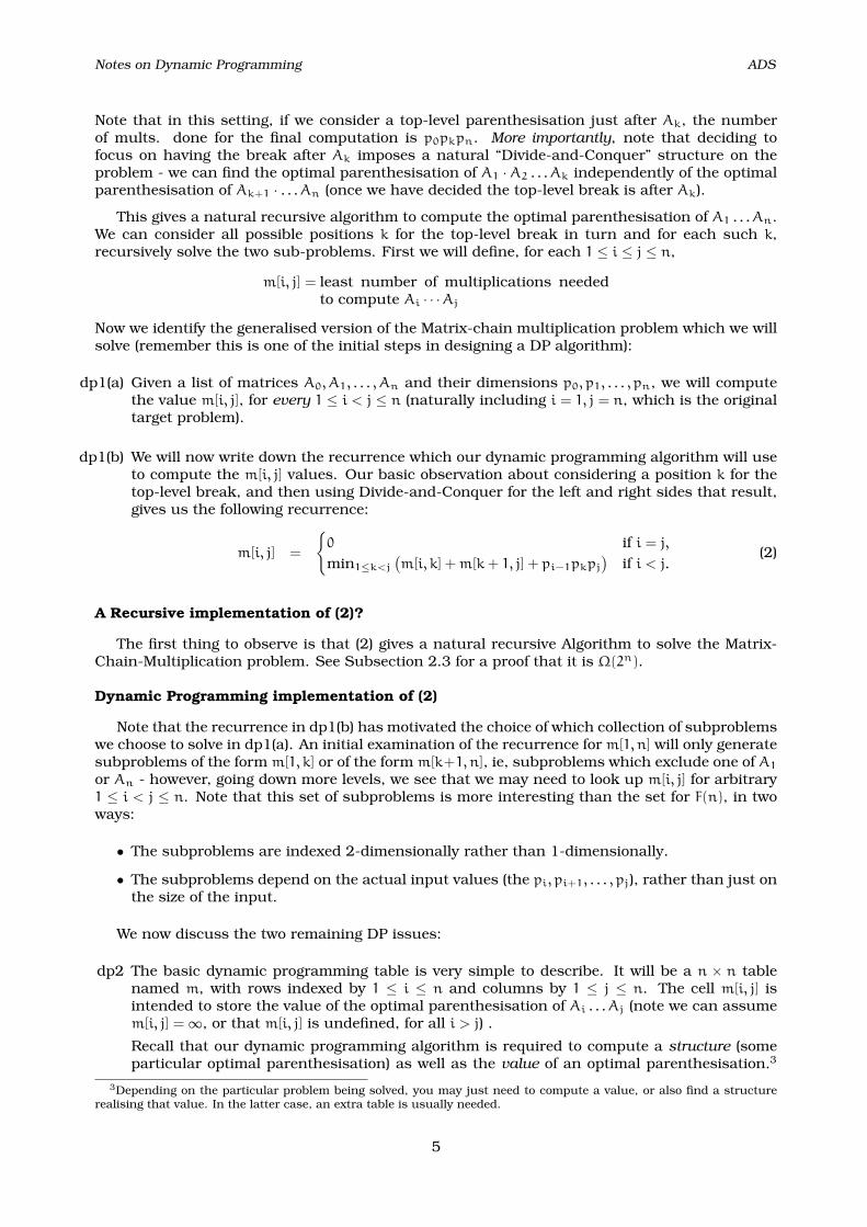
Note that in this setting, if we consider a top-level parenthesisation just after Ak, the numberof mults. done for the final computation is p0pkpn. More importantly, note that deciding tofocus on having the break after Ak imposes a natural “Divide-and-Conquer” structure on theproblem - we can find the optimal parenthesisation of A1 ·A2 . . . Ak independently of the optimalparenthesisation of Ak+1 · . . . An (once we have decided the top-level break is after Ak).

This gives a natural recursive algorithm to compute the optimal parenthesisation of A1 . . . An.We can consider all possible positions k for the top-level break in turn and for each such k,recursively solve the two sub-problems. First we will define, for each 1 ≤ i ≤ j ≤ n,

m[i, j] = least number of multiplications neededto compute Ai · · ·Aj

Now we identify the generalised version of the Matrix-chain multiplication problem which we willsolve (remember this is one of the initial steps in designing a DP algorithm):

dp1(a) Given a list of matrices A0, A1, . . . , An and their dimensions p0, p1, . . . , pn, we will computethe value m[i, j], for every 1 ≤ i < j ≤ n (naturally including i = 1, j = n, which is the originaltarget problem).

dp1(b) We will now write down the recurrence which our dynamic programming algorithm will useto compute the m[i, j] values. Our basic observation about considering a position k for thetop-level break, and then using Divide-and-Conquer for the left and right sides that result,gives us the following recurrence:

m[i, j] =

0 if i = j,min1≤k<j

(m[i, k] +m[k+ 1, j] + pi−1pkpj

)if i < j.

(2)

A Recursive implementation of (2)?

The first thing to observe is that (2) gives a natural recursive Algorithm to solve the Matrix-Chain-Multiplication problem. See Subsection 2.3 for a proof that it is Ω(2n).

Dynamic Programming implementation of (2)

Note that the recurrence in dp1(b) has motivated the choice of which collection of subproblemswe choose to solve in dp1(a). An initial examination of the recurrence for m[1, n] will only generatesubproblems of the form m[1, k] or of the form m[k+1, n], ie, subproblems which exclude one of A1

or An - however, going down more levels, we see that we may need to look up m[i, j] for arbitrary1 ≤ i < j ≤ n. Note that this set of subproblems is more interesting than the set for F(n), in twoways:

• The subproblems are indexed 2-dimensionally rather than 1-dimensionally.

• The subproblems depend on the actual input values (the pi, pi+1, . . . , pj), rather than just onthe size of the input.

We now discuss the two remaining DP issues:

dp2 The basic dynamic programming table is very simple to describe. It will be a n × n tablenamed m, with rows indexed by 1 ≤ i ≤ n and columns by 1 ≤ j ≤ n. The cell m[i, j] isintended to store the value of the optimal parenthesisation of Ai . . . Aj (note we can assumem[i, j] =∞, or that m[i, j] is undefined, for all i > j) .

Recall that our dynamic programming algorithm is required to compute a structure (someparticular optimal parenthesisation) as well as the value of an optimal parenthesisation.3

3Depending on the particular problem being solved, you may just need to compute a value, or also find a structurerealising that value. In the latter case, an extra table is usually needed.

5

Notes on Dynamic Programming ADS

We will define a second table s of size n×n, where s[i, j] will store the value k of the (minimum)“top-level break” (i ≤ k < j) which will achieve a optimal parenthesisation for Ai . . . Aj.Formally,

s[i, j] = (the smallest) k such that i ≤ k < j andm[i, j] = m[i, k] +m[k+ 1, j] + pi−1pkpj.

dp3 Next we need to prescribe the order in which the table will be filled-in. To do this examinethe recurrence (2). Note that when we consider i ≤ k < j, we are guaranteed that both the“left-side” and the “right-side” will contain at least one matrix. Hence for any k considered,the subproblems referenced contain strictly fewer matrices than the current problem underconsideration. Therefore we only need organise our algorithm to compute the solutions forshorter sequences of matrices first, and once we have done that, we are guaranteed that allvalues on the right-hand side of the recurrence will be available when they are needed.

So as usual, the key to getting a good DP algorithm is to compute solutions in a bottom-upfashion.

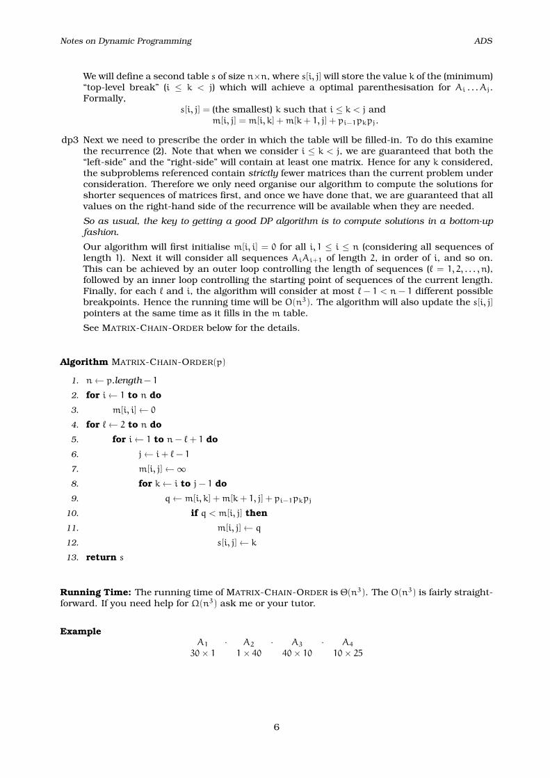
Our algorithm will first initialise m[i, i] = 0 for all i, 1 ≤ i ≤ n (considering all sequences oflength 1). Next it will consider all sequences AiAi+1 of length 2, in order of i, and so on.This can be achieved by an outer loop controlling the length of sequences (` = 1, 2, . . . , n),followed by an inner loop controlling the starting point of sequences of the current length.Finally, for each ` and i, the algorithm will consider at most ` − 1 < n − 1 different possiblebreakpoints. Hence the running time will be O(n3). The algorithm will also update the s[i, j]pointers at the same time as it fills in the m table.

See MATRIX-CHAIN-ORDER below for the details.

Algorithm MATRIX-CHAIN-ORDER(p)

1. n← p.length − 1

2. for i← 1 to n do

3. m[i, i]← 0

4. for `← 2 to n do

5. for i← 1 to n− `+ 1 do

6. j← i+ `− 1

7. m[i, j]←∞8. for k← i to j− 1 do

9. q← m[i, k] +m[k+ 1, j] + pi−1pkpj

10. if q < m[i, j] then

11. m[i, j]← q

12. s[i, j]← k

13. return s

Running Time: The running time of MATRIX-CHAIN-ORDER is Θ(n3). The O(n3) is fairly straight-forward. If you need help for Ω(n3) ask me or your tutor.

ExampleA1 · A2 · A3 · A4

30× 1 1× 40 40× 10 10× 25

6

Notes on Dynamic Programming ADS

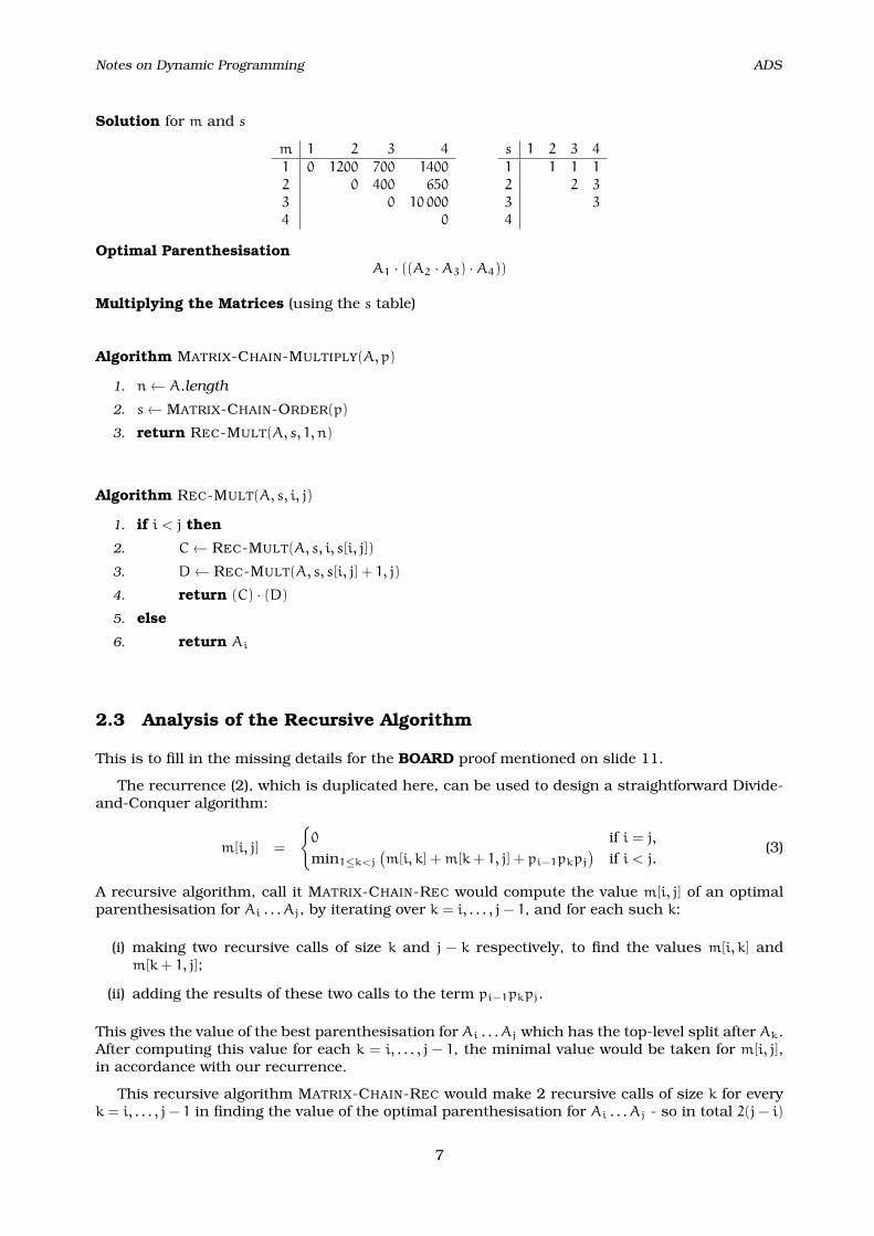
Solution for m and s

m 1 2 3 4

1 0 1200 700 14002 0 400 6503 0 10 0004 0

s 1 2 3 4

1 1 1 12 2 33 34

Optimal ParenthesisationA1 · ((A2 ·A3) ·A4))

Multiplying the Matrices (using the s table)

Algorithm MATRIX-CHAIN-MULTIPLY(A,p)

1. n← A.length

2. s← MATRIX-CHAIN-ORDER(p)

3. return REC-MULT(A, s, 1, n)

Algorithm REC-MULT(A, s, i, j)

1. if i < j then

2. C← REC-MULT(A, s, i, s[i, j])

3. D← REC-MULT(A, s, s[i, j] + 1, j)

4. return (C) · (D)

5. else

6. return Ai

2.3 Analysis of the Recursive Algorithm

This is to fill in the missing details for the BOARD proof mentioned on slide 11.

The recurrence (2), which is duplicated here, can be used to design a straightforward Divide-and-Conquer algorithm:

m[i, j] =

0 if i = j,min1≤k<j

(m[i, k] +m[k+ 1, j] + pi−1pkpj

)if i < j.

(3)

A recursive algorithm, call it MATRIX-CHAIN-REC would compute the value m[i, j] of an optimalparenthesisation for Ai . . . Aj, by iterating over k = i, . . . , j− 1, and for each such k:

(i) making two recursive calls of size k and j − k respectively, to find the values m[i, k] andm[k+ 1, j];

(ii) adding the results of these two calls to the term pi−1pkpj.

This gives the value of the best parenthesisation for Ai . . . Aj which has the top-level split after Ak.After computing this value for each k = i, . . . , j − 1, the minimal value would be taken for m[i, j],in accordance with our recurrence.

This recursive algorithm MATRIX-CHAIN-REC would make 2 recursive calls of size k for everyk = i, . . . , j− 1 in finding the value of the optimal parenthesisation for Ai . . . Aj - so in total 2(j− i)

7

Notes on Dynamic Programming ADS

recursive calls at the “top level” (an unusually high number compared to other recursive algs wehave seen); also it will evaluate j− i− 1 different pi−1pkpj terms at the “top level”.

We now show the running time of this proposed recursive algorithm MATRIX-CHAIN-REC isexponential (Ω(2n) in fact) in the number of matrices j − i + 1 under consideration. We writen = j − i + 1, in designing our recurrence. The running time TM-C-R(n) satisfies the recurrencewhich was given on slide 11 of lectures 10.11:

TM-C-R(n) =

Θ(1) n = 1∑n−1

k=1

(TM-C-R(k) + TM-C-R(n− k)

)+Θ(n) n ≥ 2

Note that the k in this running-time recurrence is not the same k in our recurrence for m[i, j]. Here itdenotes the SIZE of the left-hand recursive call. It actually maps to k − i + 1 in the terms of m[i, j]recurrence.

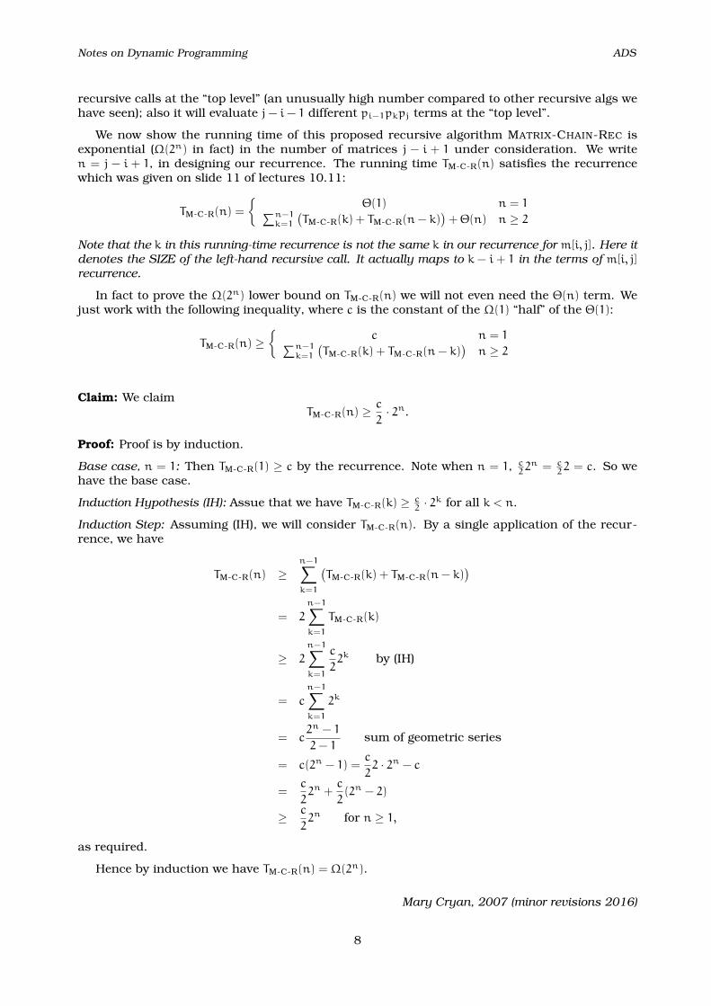
In fact to prove the Ω(2n) lower bound on TM-C-R(n) we will not even need the Θ(n) term. Wejust work with the following inequality, where c is the constant of the Ω(1) “half” of the Θ(1):

TM-C-R(n) ≥

c n = 1∑n−1k=1

(TM-C-R(k) + TM-C-R(n− k)

)n ≥ 2

Claim: We claimTM-C-R(n) ≥

c

2· 2n.

Proof: Proof is by induction.

Base case, n = 1: Then TM-C-R(1) ≥ c by the recurrence. Note when n = 1, c22n = c

22 = c. So we

have the base case.

Induction Hypothesis (IH): Assue that we have TM-C-R(k) ≥ c2· 2k for all k < n.

Induction Step: Assuming (IH), we will consider TM-C-R(n). By a single application of the recur-rence, we have

TM-C-R(n) ≥n−1∑k=1

(TM-C-R(k) + TM-C-R(n− k)

)= 2

n−1∑k=1

TM-C-R(k)

≥ 2

n−1∑k=1

c

22k by (IH)

= c

n−1∑k=1

2k

= c2n − 1

2− 1sum of geometric series

= c(2n − 1) =c

22 · 2n − c

=c

22n +

c

2(2n − 2)

≥ c

22n for n ≥ 1,

as required.

Hence by induction we have TM-C-R(n) = Ω(2n).

Mary Cryan, 2007 (minor revisions 2016)

8