Embed Size (px)
Citation preview
- ~ Nuclear PhystcJ A244 (1975) 365-434; (~) North-Holland Publhhtno Co., Amsterdam
Not to be reproduced by photoprint or microfilm without written permission from the publisher
F E W - N U C L E O N SU(3) P A R E N T A G E COEFFICH~.. N T S A N D ~ - P A R T I C L E S P E C T R O S C O P I C A M P L I T U D E S
FOR C O R E E X C I T E D S T A T E S IN s-d S H E L L N U C L E I t
K. T. HECHT and D. BRAUNSCHWEIG
Physics Department, University of Michigan, Ann Arbor, Michiaan 48104, USA
Received 3 December 1974
Abstract: The SU(6)/SU(3) factors of few-nucleon fractional parentage coefficients in ls-0d shell nuclei are calculated directly without being generated recursively from one-nucleon c.f.p. Tabulations are given for x-nucleon reduced matrix elements, (x = 4, 3, 2, 1), connecting states of high SU(3) symmetry, where the x-nucleon states are limited to states of totally symmetric space and oscillator quanta symmetry, i.e. SU(3) representations (80), (60), (40), (20) for states of space symmetries 14], [3], [2], I-1]. Together with the SU(3)/R(3) factors calculated by Draayer, these reduced matrix elements make it possible to predict spectroscopic amplitudes for reactions in which the x-nucleon groups are transferred in unexcited (0s) internal states. In a specific application, ,,-particle spectros- copic amplitudes are calculated for core-excited states in s-d shell nuclei, reached by the transfer of(0p)- t (ls0d)- 3, or (0p)- 2(1 s0d)- 2 groups in pickup reactions and (ls0d) 3(lp001 or (ls0d)2(lp0f) 2 groups in stripping reactions, where states in the final residual nuclei are approximated by SU(3) strong coupling states, (free of spurious c.m. excitation), corresponding ot the largest possible intrinsic deformations in these nuclei. The effect of a difference in ~t-particle size parameters in projectile and residual nuclei is discussed.
1. Introduction
Recent direct mul t i -nucleon transfer react ion experiments with Li o r heavy- ion projectiles have st imulated a number o f new theoretical calculat ions 1-3) o f ~t-
particle spectroscopic amplitudes. Besides a number o f specific cluster model calculat ions 1,4, 5), general theoretical formulat ions in the f r amework o f the ha rmonic oscillator shell model have now also been b rough t to a state o f development 1- a)
which makes specific calculations feasible. In all the recent formula t ions it is assumed that the or-cluster is t ransferred in an unexcited (0s) internal state, an assumpt ion which is just if ied no t only for Li induced reactions but also for direct transfer reac- t ions between heavy ions because o f the surface nature o f such reactions 2). Cal-
culations in the f ramework o f the j-j coupled shell model have been carried out by K u r a t h and Towner 2) who relate the ~-spectroscopic ampli tudes to a sum o f coupled two-neut ron and two-p ro ton spectroscopic ampli tudes by means o f a formula which is no t only convenient for calculations in heavy nuclei but directly relates properties o f ~-transfer reactions to the more familiar properties o f two-nucleon transfer
t Supported by the US National Science Foundation.
365 June 1975
366 K.T. HECHT AND D. BRAUNSCHWEIG
reactions. Their calculations also show that there is much fragmentation of the ~- transfer strength in a good j-j coupling nucleus among the many possible config- urations (JlJ2J3J4) of a given major oscillator shell. The SU(3) shell model calculations of Ichimura, Arima, Halbert, and Terasawa 1), on the other hand, show that the •-strength can be highly concentrated in a few rotational bands in a good SU(3) nucleus. In s-d shell and lighter nuclei it is therefore advantageous to calculate ~- particle spectroscopic amplitudes in the framework of the SU(3) representation of the harmonic oscillator. In this framework the overlap between an ~-cluster wave function and a four-particle shell model wave function takes an extremely simple form 1), and the calculation of ~-particle spectroscopic amplitudes is immediately reduced to a calculation of n ~ (n -4 ) particle parentage coefficients for the n valence nucleons. In the usual method of calculation such four-nucleon c.f.p, are generated recursively from one-nucleon c.f.p. Although the process is straight- forward, it is tedious and complicated by the fact that the many needed intermediate state one-nucleon parentage coefficients are not available in tabulated form in the SU(3) scheme. As a result, ~-particle spectroscopic calculations based onthe SU(3) model have been limited 1,6) to nuclei near 160. Although full four-nucleon c.f.p. have not been available for s-d shell nuclei, the SU(3)/R(3) parts of these c.f.p, are readily available through the work of Draayer and Akiyama 7. s). A recent extensive tabulation by Draayer 3) gives the full angular momentum dependence of these factors and makes possible a prediction of the relative ~-transfer strengths to dif- ferent members of a rotational band (with angular momentum projection Kj), provided the states of the rotational band are pure (or relatively pure) in their SU(3) symmetry quantum numbers. Draayer's tabulation of the angular momentum dependent (SU(3)/R(3)) factors have therefore reduced the problem to the calculation of the SU(6)/SU(3) factors of few-nucleon c.f.p, in the s-d shell. These factors are needed to predict absolute values of ~-spectroscopic amplitudes, to assess quan- titatively the effects of SU(3) representation mixing in the ground state rotational bands, and to compare the ~-transfer strengths to excited rotational bands with those for the ground state band. The latter would be particularly difficult to estimate in the framework of the j-j coupled shell model if the rotational bands are based on core excited states, such as the low-lying negative parity rotational bands in s-d shell nuclei. For ~-particle spectroscopic amplitudes to core excited states in s-d shell nuclei, the SU(3) scheme is therefore not only a powerful calculational tool but is vital to furnish a reasonable description of the states themselves.
It is the purpose of this contribution to exhibit a method by which the SU(6)/SU(3) factors for few-nucleon c.f.p, in the s-d shell can be calculated without being generated recursively from one-nucleon c.f.p, and without a chain calculation. A brief discus- sion of spectroscopic amplitudes for few-nucleon transfer processes and their relation to few-nucleon parentage coefficients is given in sect. 2. Some of the details of the method of calculation are given in an appendix together with a fairly extensive tabulation of four-, three-, two- and one-nucleon reduced matrix elements con-
SU(3) PARENTAGE COEFFICIENTS 367
netting states of high SU(3) symmetry (large SU(3) quantum numbers (2#)). In these tabulations the four-, three- and two-nucleon states corresponding to the transferred cluster are limited to states of totally symmetric space and oscillator quanta sym- metry, i.e. space symmetry quantum numbers [4], [3], and [2], respectively, with corresponding SU(3) symmetry (80), (60), and (40).
Sect. 3 takes up the calculation of ~t-particle spectroscopic amplitudes for core excited states in s-d shell nuclei; i.e. et-particie spectroscopic amplitudes for the transfer of (0p) -1 (ls0d) -a, (0p)-2(ls0d)-2, ... clusters in pickup reactions, and (ls0d)a(lp0f)l,(ls0d)2(lp0f)2, .. .clusters in stripping reactions. The general formulation is given for both the SU(3) weak-coupling 9- ix) and SU(3) strong- coupling t 2) models. Numerical estimates, however, are based on the SU(3) strong- coupling model since it is somewhat simpler and can be expected to give a good estimate of ~-transfer strength to core excited states in s-d shell nuclei. It is also closely related to the generalized quartet model of Harvey 13) which can be used as a guide to the most-likely low-lying particle-hole excitations in such nuclei. The SU(3) strong-coupling scheme has an additional advantage. Most states with large values of the SU(3) quantum numbers (2#) are entirely free of spurious c.m. ex- citations. In those few cases where spurious c.m. excitations must be considered, the SU(3) strong-coupling scheme also furnishes the simplest calculational frame- work for the elimination of such excitations 17). The few states of spurious c.m. excitation which are needed in this investigation, are tabulated in an appendix, together with a discussion of the limits on the SU(3) quantum numbers 2, # which delineate the regions free of spuriosity.
The four-nucleon c.f.p, tabulated in this contribution are limited to those needed for the calculation of ~-transfer amplitudes under the assumption that the size of the transferred ~-cluster is the same in both projectile and residual nuclei. The effect of a difference in size on ~-spectroscopic amplitudes has been discussed bv lchimura e t al . ~). Since their formulation involves relatively complicated Talmi-Moshinsky recoupling transformations, a simpler derivation leading to somewhat more general results is given in an appendix. However, these results in no way change the con- clusions of ref. 1) that the differences in ~-cluster size should lead to only small ef- fects on observable phenomena in s-d shell nuclei.
2. Few-nucleon spectroscopic mplitudes
The differential cross section for the direct x-nucleon transfer reaction A(a, b)B, with B = A + x , and a = b + x, is in general given by a coherent superposition of structure (spectroscopic) factors, B, and kinematic (reaction mechanism) factors, ft. Adhering strictly to the notation of ref. 2):
d°'(A ~ B ) = #'/'tb Kb 2 J e + l ~.I E B~sb~ffl~s~t ~r" (1) dr2 (2nh2) 2 K~ (2JA+I)(2j,+I) : - M OLOE "
368 K.T. HECHT AND D. BRAUNSCHWEIG
It is assumed that the states of the transferred x-nucleon group can be described in the framework of the harmonic oscillator shell model, and Q = 2N+L gives the number of oscillator quanta for the relative motion of the x-nucleon cluster with respect to nucleus A. If the intrinsic state of the transferred x-nucleon cluster has an angular momentum, j~, then Jx =ix+L, with similar definitions for Q, E, J~, for the x + b nucleon projectile. The structure factors B aL' QL are given in terms of the two spectroscopic amplitudes A(B ~ A + x) and A(a ~ b +x) and in general involve a sum over the intrinsic states of the transferred x-nucleon group and angular momentum recoupling coefficients [for details, see ref. 2)]. If the x-nuc'I~on group is transferred in an unexcited internal state with zero intrinsic angular momentum, such as the (0s) internal state of an unexcited or-cluster, the structure factor, B, is given by a simple product of the two spectroscopic amplitudes. In this case the dif- ferential cross section for the transfer reaction is also given by a product of a single spectroscopic factor and a reaction mechanism factor, as in the case of a direct one- nucleon transfer reaction (provided the target and residual nuclear states are not mixtures of core excitations with different particle-hole numbers).
The present investigation will be concerned solely with the spectroscopic am- plitudes A(B---, A+x) . These spectroscopic amplitudes are determined by three types of factors. Again in the notation of ref. 2), [see also ref. 1)], the spectroscopic amplitude A(B ~ A + x) is given by
Amm(B ~ A+x) = ~,B---~,] ~' (O(B):~IIz*rJ~[IO(A)J") F
x (¢ i . t . (~x)~NL(gx) l~(~x) ) . (2)
The first factor, given by the mass ratio, B/(B-x), comes from the generalized Talmi-Moshinsky transformation which relates the wave function em.(rx_A), describing the relative motion of the x-nucicon cluster with respect to the center of mass of nucleus A, to the wave function ¢~m.(Rx), describing this motion with respect to the center of the harmonic oscillator potential well 1). (Since Q = 2N+ L may be large this factor can be important, although it is often ignored in two-nucleon transfer processes in heavy nuclei.) The second factor, the double-barred matrix dement, is the reduced matrix element of an x-nuclcon creation operator, X*, where the x creation operators are coupled to total angular momentum J~ and are specified by additional quantum numbers F. The last factor, the "G" factor of refs. 1, 2), is the overlap of the x-nucleon duster wave function and the x-particle shell model wave function, specified by quantum numbers, FJ~. The coordinates, ~ , describe the internal degrees of freedom of the x-nucleon cluster, whereas the shell model coordinates, ~x, describe the motion of these x nucleons relative to the well center. If shell model wave functions are specified in j-j coupling, this overlap is different from zero for many possible x-particle shell model states, and the spectroscopic amplitude involves a summation over many states, F, specified, for example, by the
SU(3) PARENTAGE COEFFICIENTS 369
single-particle quantum numbers nl l l j l . . . . . nxlxj x, with additional intermediate- coupling angular momentum quantum numbers such as J , 2, J34 [see ref. 2)]. In the framework of the SU(3) representation of the harmonic oscillator shell model the overlap for the x-particle group takes a very simple form. If the x-particle cluster is transferred in an unexcited (0s) internal state, and if the oscillator size parameters for the x particles is assumed to be the same in the a-nucleon projectile and the B- nucleon residual nucleus, the above summation over F collapses to a single term. For x = 4, this overlap or G-factor has been given by Ichimura et al. 1), and has the simple form
V Q' l'F 4, ], G = 14aq,!~2iqa!q4i_ ] Latb!c!d ! 6U-lt,1fs0fro6Q,2s+Lfaa6,o (3)
for four-nucleon transfers in the configuration q l q 2 q a q a - l - q ~ q C w ~ (with a + b + c + d = 4), where qi = 2ni + l~ is the number of oscillator quanta of the ith transferred particle, and Q = q l + q 2 + q 3 + q 4 = 2 N + L is the total number of oscillator quanta in the transferred cluster. [For the transfer of a (ls0d)a(lp0f) 1 four-particle cluster, for example, a = 3, b = 1, c = d = 0, with ql = q2 = q3 -- 2 ( = qu), q4 = 3 ( = qv); and Q = 9.] In eq. (3), [f] stands for the space symmetry quantum numbers, given in terms of the usual partition numbers; (2#) are the Elliott SU(3) quantum numbers; [the notation follows that of refs. 1, a)]. In eq. (2), a summation over more than one state F will occur only in the extremely rare cases when the final state in nucleus B can be reached from the initial state in nucleus A by more than a single configuration with the same Q; e.g. the configurations (1 sOd) 2 (lp0f) 2, and (ls0d)3 (2sld0g) 1, both with Q = 10; [the K = 0 ÷ band 15) in 2°Ne with band head centered on the wide level at 8.3 MeV, may be such an example; see ref. 1) and sect. 3]. For x = 3, (again for a three-nucleon cluster transferred in a (0s) internal state with oscillator size parameter properly matched between a- and B-nucleon systems), the three-particle overlap factor for the transfer into the configuration qlq2q3 =- q~uq~uqCw with a + b + c = 3, is
[ Q! ]½[ 3! 7 ½ G = k3eq,.~q2!q3ij L ~ _ ] 6tY'ta16s~fr~fe'2N+L6ae6"° (4)
(see appendix D). In the framework of the SU(3) representation of the harmonic oscillator, the
calculation of the x-particle spectroscopic amplitude, Am.ss, is thus reduced to the calculation of the double-barred matrix element of eq. (2) which, except for trivial factors, is an n ~ n - x parentage coefficient for the n valence nucleons of nucleus B. The calculation of these coefficients is simplified greatly if the double-barred matrix element is factored into an SU(3)/R(3) factor and a second factor inde- pendent of SU(3) subgroup labels (and hence independent of all angular momentum quantum numbers); particularly since the SU(3)/R(3) (angular momentum de- pendent) factors are readily available through the recent work of Draayer 3, 7).

370 K.T. HECHT AND D. BRAUNSCHWEIG
The states of nuclei A and B are specified by [fJo~(2#)flSTr.tLJ, or alternately by [f]o~(2#)flSTxsr.sJ, [see ref. 3)], where I f ] and (4#) label the space and SU(3) symmetry, respectively; ct is used to distinguish multiple occurences of a given (2#) in a specific If], / /distinguishes multiple occurences of ST in the spin-isospin sym- metry [.97] contragredient to [_f]; (labels ct and/or / /a re usually omitted when not needed). The labels x are generalizations of the angular momentum projection labels K used by Elliott where the x refer to orthogonalized states [see refs. 3,s)], and where KL (or XL), Ks, Ks refer to the projections of the angular momenta L, S, J. For states labeled by [_f]o~(2#)[3STxsxsJ, the reduced (double-barred) matrix element of the x-nucleon creation operator of eq. (2) can be factored into a triple- barred matrix element, (independent of all SU(3) subgroup labels) and an SU(3)/R(3)
a angular momentum factor, ANLSJ, in the notation of Draayer 3),
( [f']~'(2'#')/~'S~ Tg M~B x~ x9 J~llx*t~]¢Q°~t'SJrll[f]0~(2#)~SA TAMr,, Xs Xs JA)
= ARLsJ([f']o~'(A'K)~'S'sTglIIztt'~J¢e°)STIII[f]o~(A#)~SATA)
X (TAMTA TMTIT'BM'rB). (5)
The operator X t'~lt = [a + x a + x a + x a+], e.g., is built from four nucleon cre, ation operators, a +, properly coupled to resultant quantum numbers [4](QO)LSJT. The factor ARLss gives the dependence on all SU(3) subgroup labels and has been eval- uated and tabulated by Draayer 3)
ARLsJ = ~ c,,,..t,,.C,,,,q X S ((2#)x,g^; (Q0)gll(2'#')r~.gs). (6) ~LLA~'LL'~ k LB SB t B
Here X( ) is an angular momentum 9-j coefficient in unitary form; the double- barred coefficient is an SU(3)/R(3) Wiguer coefficient; and the C~,.L are the trans- formation coefficients from states of good tct LSJ to states of good XsxsSJ; [see ref. a)]. In s-d shell nuclei the triplebarred matrix element of eq. (5) can further be expressed in terms of the conventional SU(6)/SU(3) and SU(4)/ST factors of an n ~ n - x parentage coefficient a, 16)
<[f']o~'(2' #')fl'S's T~lllxux](Q°)srlll[f]o~(2#)flSA TA> = CD, (7a)
where the "C" and "D" factors are given in terms of the n --.,. ( n - x ) c.f.p, by
C - < [ f ' ]= ' (2 '# ' ) l l IIz*t"J(a°~ll I I [ f ] a ( 2 # ) )
n! dims,_ , [ f ] l~ . . . . . . . . - (n-~)!x! ~ j ~'LY-lZttz#)' [x](Q0)l}['f']~t'(2'/l)>, (7b)
D = ([7]flSA TA; [lX]STI}[7']~'S~ Tg). (7c)
SU(3) PARENTAGE COEFFICIENTS 371
The D-factor is the spin-isospin part of the n --* n - x c.f.p, which can be identified , l
as a reduced SU(4)/[SU(2)s x SU(2)r] V~igner coefficient for the supermultiplet scheme 17). For x = 4 the representation [ 14] corresponds to the scalar representation of SU(4), (with S = T = 0); and the SU(4) Wigner coefficient has the trivial value + 1, (provided [_~'] = [_.7] ; S~ = SA, T~ = TO. For x = 3, 2, 1, and most rep- resentations [_]~] of interest, these coefficients can be obtained from the tabulations of ref. 17) and are given as part of the tabulations of appendix A.
The C-factor is chosen to include, besides the SU(6)/SU(3) part of the s-d shell c.f.p., the binomial coefficient (~) and the dimension factors, dim I f ] . Here, dims,_x [_f] is the dimension of the representation [.f] of the symmetric group S,-x, the permutation group for n - x particles, described by the partition numbers [_f]; similarly for dims, I f ' ] for the representation I f ' ] of S,. (Note that the dimensions of the totally symmetric states Ix] are dimsx [xl = 1.) If the x nucleons are transferred into or out of the (0p) shell, eqs. (7) hold if the SU(6)/SU(3) part of the c.f.p, is replaced by + 1. The (0p) shell has been discussed by Kurath is). If the nucleons are transferred into or out of the (0flp) shell, the c.f.p, ofeq. (7b) must be interpreted as the SU(10)/SU(3) factor of the space part of the full c.f.p. Since both SU(4) and SU(3) subgroup labels have been factored out of the matrix element for the x-nucleon creation operator to reduce it to the C-factor, it will also be useful to denote this as the quadruple-barred matrix element of the operator X*-
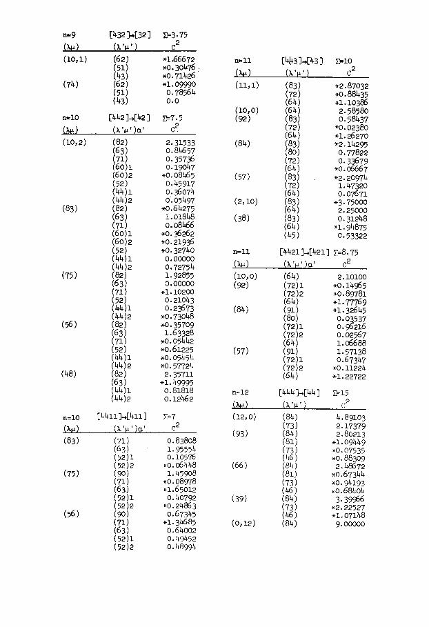
Fairly extensive tabulations of the C-factors for x-partiele transfers of (ls0d) shell nucleons are given in appendix A for x = 4, 3, 2, and 1. Some of the details of the method of calculation are also presented there. Although the method of calcula- tion can be applied equally well to parentage coefficients corresponding to x-particle transfers in excited states, with (2x#x) ~ (Q0), the tabulations of appendix A are limited to those needed for the transfer of x-nucleon dusters in unexcited states, corresponding to space symmetry quantum numbers [4], [3], [2], and [1], respec- tively, with corresponding SU(3) symmetries (80), (60), (40), and (20).
Using the sum rules for the R ANLsa factors [see eqs. (4.2) and (4.3) of ref. a)], the C-, D-, and G-factors can be used to determine the total spectroscopic strength for pickup or stripping reactions to states of specific SU(3) symmetry. For the pickup of an x-nucleon cluster
(B(2'#') ~ A(2#)) = C 2 D 2 G 2 ( T A M r A T M r [ T ~ M ~ . 8 ) 2, pickup
(8)
where this pickup sum rule refers to the summed strength for transitions from a specific rotational state in the representation 0 '# ' ) of nucleus B (with fixed x~ xj, J~, e.g.), to all rotational states of the representation (2#) in nucleus A (all possible x s x j , and JA) via all possible L- and J-transfers of an x-nucleon cluster of fixed space symmetry [x] and SU(3) quantum numbers (Q0), and specific S, T, and M r. Simi- larly,
372 K. T. HECHT AND D. BRAUNSCHWEIG
(A(Z/1) - , stripping
(-B~--X) (2 TM T, 'M' \ 2 2Sh+1 dim(2'/1') (9) "~- T S Tn/ 2SA+ 1 dim(2/1) '
where d im(2/1)=~2+l) ( /1+l ) (2+/1+2) , is now the dimension of the SU(3) representation, and the stripping sum rule refers to the summed strength for tran- sitions from a specific rotational state in the representation (2/1) of nucleus A to all rotational states of the representation (2'/1') of nucleus B, again via all possible L- and J-transfers of an x-nucleon cluster with fixed Ix], (2~/1~) = (Q0), S, T, and M T.
To gain a feeling for the relative importance of C-factors for different transitions it is useful to compare these with a sum rule for transitions from a fixed state (2'/1')S~ T~r'sX'~J ~ of space symmetry [.f'] in nucleus B to all states of space sym- metry [ f ] in nucleus A via transfer of an x-nucleon cluster of fixed space symmetry Ix] (totally symmetric in its space wave function), but with all possible (2~/1~), L, S, and T. This is given by the sum rule for the triple-barred matrix element
Y, (If'] [ f ] +
([f ' ]~'(,~' /1')fl'S'B T~III2:e"J~x"x)pSTIII[f ]~(A/1)flSA TA) 2 ( ~ . x p x ) p S T
dims, i f , ] •
These sums, ~ , are tabulated in appendix A at the head of each table of C- and D- factors and can tell at a glance what fraction of the total pickup strength from a specific state [_f'](2'#') is concentrated in transitions to a specific representation (2#) of [ f ] . Note, however, that the sum, ~2, contains strength from x-nucleon clusters in internally excited states with (2~/1x) ~ (Q0). For the transfer of four nucleons from the ls0d shell, for example, with space symmetry [4], i.e. with the spin-isospin structure of a real e-particle, this sum would in general contain transfers of four- nucleon clusters in SU(3) states (Jl~/1x) = (42), (04), and (20), as well as those for the "e-cluster" states with (Ax/1x) = (80). (The label p, needed only for (2x/ix) 4 ~ (QO), is defined in appendix A.)
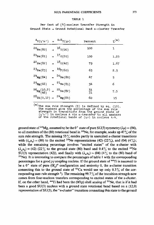
It is interesting to note that a large fraction of the summed strength, ~ , for [4] nucleon pickup is concentrated in the e-cluster transitions from the ground state to the ground state rotational band in all good SU(3) nuclei in the first half of the (ls0d) shell. The numbers are collected in table 1, under the assumption that the ground states of the target nuclei and the ground state bands of the residual nuclei shown are pure in their SU(3) quantum numbers. Table 1 shows both the sum, ~, of eq. (10) and the percentage of this summed strength which resides in the ground state to ground state rotational band transitions. The pickup strength from the
SU(3) PARENTAGE COEFFICIENTS
TABLE 1
Per Cent of [4]-nucleon Transfer Strength in
Ground State . Ground Rotational Band a-cluster Transfer
373
AX(k'~') ~ A-~Y(k~) Percent E (a)
2ONe(80) . 160(00 ) I00 1
2X~e(81) ~ 17o(2o) 1oo 1.25
22Ne(82) * 180(40) 79 1.67
23Na(83) ~ 19F(60) 63 2.5
24Mg(84) ~ ~ONe(80) 47 5
25Mg(66) ~ 21Ne(81) 34 6
26. (10,2) 22Ne(82) 31 Mg(48) 4 31 7.5
28S1(0,12) * 2~Mg(84) 60 15
(a)The sum rule strength (Z) is defined by eq. (i0). The numbers give the percentage of the sum rule strength in transitions from the ground state of (k'~') in nucleus A via a-transfer'to all members of the rotational bands of (kg) in nucleus A-A.
ground state of 24Mg, assumed t9 be the 0 + state of pure SU(3) symmetry (2#) = (84), to all members of the (80) rotational band in 2°Ne, for example, soaks up 47 % of the sum rule strength. The missing 53 % resides partly in unexcited 0t-cluster transitions with (;t~#~) = (80) to the excited 2°Ne representations (42) (22%), and (04) (4%); while the remaining percentage involves "excited states" of the ~-cluster with (2~/4) = (42) (22% to the ground state (80) band and 0.4% to the excited 2°Ne SU(3) representation (42)), and finally with (;%#~) = (04) (4% to the (80) band of 2°Ne). It is interesting to compare the percentages of table 1 with the corresponding percentages for a goodj-j coupling nucleus. If the ground state of 44Ti is assumed to be a 0 + state of pure (0f~) 4 configuration and seniority 0, the ~t-cluster transition connecting this to the ground state of 4°Ca would use up only 0.3 % of the cor- responding sum rule strength 2). The remaining 99.7 % of the transition strength now comes from four-nucleon transfers corresponding to excited states of the or-cluster. If, on the other hand, 44Ti had been the (0flp) shell analog of 2°Ne, that is if it had been a good SU(3) nucleus with a ground state rotational band based on a (12,0) representation of SU(3), the "~t-cluster" transition connecting this state to the ground
374 K. T. HECHT AND D. BRAUNSCHWEIG
state of '~°Ca would have used up 100,%o of the summed strength. (Since this is a hypothetical remark, we shall not be concerned with the fact that 44Ti does not present us with a stable target for a pickup reaction to 4°Ca.) The numbers again emphasize the close relationship between the SU(3) representation and the cluster model. The numbers also show that small admixtures of lower (2#) representations into the representations of high SU(3) symmetry may be relatively less important in their contribution to the 0t-transfer strength to the ground state bands, since they are generally weighted by smaller C-factors.
3. Alpha-particle spectroscopic amplitudes for core-excited states in s-d shell nuclei
The C-factors tabulated in appendix A can be used together with the factors, R Am.ss, tabulated by Draayer 3) to calculate any g-particle spectroscopic amplitude
for a transfer involving a (1 s0d) 4 cluster. Since core excitations give rise to low-lying bands in many s-d shell nuclei, g-particle spectroscopic amplitudes for the transfer of (0p)- l ( ls0d)-3,(0p)-2( ls0d) -2, .. . clusters in pickup reactions, and (ls0d) 3 (lp0f) 1, (ls0d) 2 (lp0f) 2, . . . clusters in stripping reactions may also be of particular interest. Since the G 2 factors for such transfers are favored by the factor (4 !/a !b !), [see eq. (3) and table 1 ofref. 1)1 such transfers may compete favorably with transfers into or out of the (ls0d) valence shell, provided the corresponding parentage coeffi- cients are sufficiently large. Transfers of (1 sod) ° (lp0f) ~ clusters may also be strongly favored over (1 sod) 4 clusters by the kinematic factors for the direct reaction process since the wave functions ¢'NL(ro,) for the relative motion of the g-cluster will be larger in the surface region if the transfer involves a cluster with a larger number of quanta Q = 2N+ L. Since both the SU(3) weak-coupling and SU(3) strong-coupling models have been used to describe core-excited states in s-d shell nuclei, the formulation will be given for both coupling schemes.
The work of Ellis, Engeland and collaborators 10.11) shows that the weak-coupling model furnishes a good approximation for particle-hole excitations in nuclei near a60, particularly for configurations (0p)"' (ls0d)"', (with nl < 12). In the SU(3) weak-coupling model the n = nt +n2 particle states are specified in a basis such as
I(Opy"[f~]a~(,h zl)xL, L1 sl Ja T1; (ls0d)"~[f2]a.2(22/~2)~z.~ L2 $2 J2 T2; JM, TMr) ,
with J = J1 +J2 , T = T 1 + T 2 ; that is, only the total angular momenta and isospins of the particle and hole configurations are coupled to resultant J and T. The space symmetry and SU(3) quantum numbers for both particle and hole configurations separately are assumed to be good quantum numbers in some zeroth approximation. To evaluate the reduced matrix element of the four-nucleon creation operator, Z tE4]tQ°), it is only necessary to couple the creation operators for the two separate shells [to space symmetry [4], SU(3) representation (Q0), total L, and S = T = 0] :
SU(3) PARENTAGE COEFFICIENTS
Xft,tltQO) = ~ <(Q10)/1 ; (Q20)lall(QO)g><[lX,]st; [lX~]stl}[l+]00> S=T--O,LM | 1 1 2 ~
375
x ~ (lltri~Izm2[LM>(sm,,sm,,lOO>(tm,,t~lO0> (11) pnords lmt i
X ~'t [xd(Qt O) ~'t [xM(Q20) /~/ lml~rt$1tml 1 ~'|2HIlWlIIJ2II~I/2 '
where xz + x 2 = 4, Q1 = x t q l , Q2 = x2q2, Q = QI-I-Q2 • The double-barred coef- ficient is an SU(3)/R(3) Wigner coefficient. [Its algebraic form is known, Sharp et aL 19).] The second coefficient is an SU(4)/ESU(2)x SU(2)] Wigner coefficient Uthe D-factor of eq. (7c)]. With x = 1, 2 , 3, these coefficients have the simple values
( 1 11 13 11 14 00> = /l13-111rlqlllHl+-I00> [ 3~[ 3~1}[ ] +1, X L J 2 2 L J 2 2 ' J L J = +1,
<[12]10[12]101}[1"]00> = +x/½, <[12]01[12]011}[1+]00> = --x/~2.
Straightforward angular momentum recoupling gives the result
<(q ~)"' +~'[f~]ot~(2~ #~)r~, E~ S'~ J~ T~; (q2~ '= + ~'[f~]a~().~ #'2)x'L, I, 2 S' z J'2 T~; J'.'TglI
X r~.tixd(Qlo) v ~?[x2-1(Q2o)l[4l(QO) I_z ^~ 3 3s=r=o,L (12)
x II(qa)"'[A] ax (,~x #l)xL, L1 $1 J1 TI; (q2)n2[f2] a2 (22/'t2)XL= L2 $2 J2 T2; JA TA>
T 1 ' T1N~ /S 1 S'IN~ f L 1 11 Y_,,'~ fLAL = ~ X T z t Z~ y I S 2 s S I 2 ~ X I L 2 12 L 2 J X I S A 0 SIB
~ t l l 1 2 L^SALhS~ ' T a 0 TB,/ ~ S a 0 S'Bf \ L A L E B / \JA L J ~ /
s, x, 2 s; x X L 2 S 2 Jz S'2 J'2l<[l~']st[l"]stl}[l+]O0>
\ L A SA J A / \Ig n S~ J 'B/
• 0 t t t r . ! t t t x ((21/zl)~:r.,Lz, (Qz)/dl(Xt #l)xr, El>((,~2/22)/CL2L2, (Q20)/21I(A2#2)rcL2/-52>
× <(Q10)11 ;(Q2 o)I211(QO)L><[f~]~'d& #'ds'~ T;lllz~tx'lte'°)lll[A]al(Ax ~l)Sx 7"1>
x < [/~]~k(,~ tt~)S~ Tilllz,+,tx~lt~°)lll[A]~,(,t2 ~2)S2 T2 >. The X-coefficients are again angular momentum 9-j coefficients in unitary form. The triple-barred reduced matrix elements can be read from the tables of C- and D- coefficients in appendix A, and the SU(3)/R(3) Wigner coefficients are available through the code of Akiyama and Draayer 7).
Since the SU(3) strong-coupling model leads to somewhat simpler results, it is the model which will actually be used to give numerical estimates of the a-particle spectroscopic amplitudes for core excited states in s-d shell nuclei. The SU(3) strong- coupling model is also somewhat closer not only to the cluster model ~) but to the self- consistent deformed oscillator model 20) or any model in which the rotational states are projected from intrinsic oscillator states such as those pictured in the generalized
376
I pOf {
I$Od
K. T. HECHT AND D. BRAUNSCHWEIG
[:,ol].[ [ 21o ]J e . ~ , , . I / 2
. [3oo] ~ . e , , - o
[oo211
[ozo]J [ I o l ] l
. . . . [ , ,o]J ~ " ' A - , / z [zoo] e . 4 a - o
[ool ] l opl ~ [olo]J" e .-a ~ . 1 / 2
[ - - * - - - , , - , , - - , , - - - [ I o o ] ~ . 2 A . o
o , ~ [ o o o ] ~ . o a - o [n=n, ny]
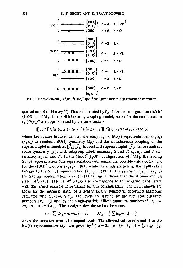
Fig. 1. Intrinsic state for (0s)*(0p)12(ls0d)V(lp0f) / configuration with largest possible deformation.
quartet model of Harvey 13). This is illustrated by fig. 1 for the configuration ( l s0d) 7 (lp0f) 1 of 24Mg. In the SU(3) strong-coupling model, states for the configuration (ql) "1 (q2)"" are approximated by the state vectors
I[(ql)"[f~]~a(21 #1) × (q2)"2[f2]~.2(2z kt2)][f](2#)~sSTMr, xjJMs),
where the square bracket denotes the coupling of SU(3) representations (2~#1) (22#2) to resultant SU(3) symmetry (2#) and the simultaneous coupling of the supermultiplet symmetries [:7] [37'2] to resultant supermultiplet [jz-j, hence resultant space symmetry [_f]; with subgroup labels including S and T, Xs, Xa, and J, (al- ternately rL, L, and J). In the ( l s0d) 7 ( lp0f ) 1 configuration o f 24Mg, the leading SU(3) representation (the representation with maximum possible value of 22+ #), for the ( l s0d) 7 group is (21#1) = (83), while the single particle in the (lp0f) shell belongs to the SU(3) representation (22#2)= (30). In the product (2x/q)x (22#2) the leading representation is (2#)= (I 1,3). Fig. 1 shows that the strong-coupling state 11,453](83)× I-1](30)]146](11,3) also corresponds to the negative parity state with the largest possible deformation for this configuration. The levels shown are those for the intrinsic states of a nearly axially symmetric deformed harmonic oscillator with co z < o9 x ~ coy. The levels are labeled by the oscillator quantum numbers [n=nxny] and by the single-particle Elliott quantum numbers 21) ~,.p.--- 2n=- n x - ny and As.p.. The configuration shown has the values
e = Z (2nz- nx - ny) = 25, Ma = ½ E (nx- ny) - ~,
where the sums are over all occupied levels. The allowed values of e and A in the SU(3) representation 0t/~) are given by =1) e = 2 2 + # - 3 p - 3 q , A =½1~+~p-½q,
SU(3) PARENTAGE COEFFICIENTS 377
with 0 _-<p _-< 2, 0 __< q _-< #; so that em, ~ = 22+#. In the coupling of [(21#l)x (22#2)](2#) = [(83)x (30)1(2#) with possible (2#)= (11,3), (10,2), (94), (91), (83), (75), (80), (72), (64), (56), only the state with (2#) = (11,3) contains e = 25, so that the many-particle state shown in fig. 1 corresponds to the intrinsic state with (2#) = (11,3). (All SU(3) states with (2#) = (11,3) can be projected from this highest weight state 21).) A weak-coupling state for (ls0d) 7 (21 #1) = (83), (lp0f) 1 (22#2) = (30), on the other hand, will contain a mixture of all the representations (11,3), (10,2), ..., (56) above, and corresponds to a smaller intrinsic deformation than the strong-coupling state. The SU(3) strong-coupling model may therefore be expected to give the better approximation for core-excited states with well defined rotational bands at a low energy of excitation. The strong coupling state with (2#) = (11,3), unlike the weak- coupling states, is also entirely free of spurious c.m. excitation (see appendix C).
In the SU(3) strong-coupling representation the reduced matrix element of the [4~ nucleon creation operator can be expressed in terms of SU(3) and SU(4) re- coupling coefficients. Straightforward generalization of the angular momentum calculus to the SU(3) and SU(4) symmetries yields
' ' ' ' 2 ' ' ' ' S T M ~ ' ' ' ttx,l<Q,o) x ttx~ltQ~o)t,*l(QOl <[[ /~](2,#l)[ f~](2#2)][f] (2#) r SXXJBIIEz Z ] s : r :o ,L
x I I [ [ f , ] (& #,)[f2](22#2)][f]().#)STMr~s~jdA)
R # t ° = ANLs:o j:L((;- #), (QO)(Z#))([f;](;.; #'dll IIz+t"~m'mll I I [A](& #1)) (13)
x <[f~](& #~)ll IIz*t~fe2°~ll I1[f2](,~2 #2)>
xXsu<,i/(Q,0 ) (Q20) (Q0) , /Xst; ,+, / [ l : ' ] [1.2] [1 +] - [0 ] ) , \ ( & # ; ) (&#~)(~'# ' )p/ k [~ ; ] [~;] [~ ]
where the coefficient R A m . s x is the Draayer factor given by eq. (6), (with S = 0). The quadruple-barred reduced matrix elements for the two major oscillator shells are given by the C-factors, [eqs. (7b) and appendix A], and the X-coefficients are generalizations to SU(3) and SU(4) of the 9-j transformation coefficient of ordinary angular momentum calculus, again in unitary form, These unitary 9-(2#) and 9-[J ~] transformation coefficients can be expressed in terms of simpler SU(3) and SU(4) Racah coefficients s, 17) by reduction formulae which are discussed in appendix B. Only very special simple cases are needed for core-excited states in s-d shell nuclei. The results for these cases are given here (for details, see appendix B).
C a s e 1 . For ~t-transfers from the configuration (ls0d)"' to the configuration (ls0d)"'+X~(lp0f)~2 (stripping reactions): [72] = [0], (22#2) = (00); [_.17] = [f : ] , (A#) = (21#1); and [_7~] = [1~2], (2~#~)= (Q20) with Q2 = 3x2- The quadruple- barred matrix element for the (lp0f) shell is + 1 ; and

378 K. T. HECHT AND D. BRAUNSCHWEIG
< [ [ f l ] (~ l ~1 )[X2](Q 2 0)] [f](2'/~')S A T A Mr , ̀ x~ x~ S~lI% t s ~ , L
x I I[[f](2~u)[0](00)] [f](2/~)S A T^ Mr , ̀ x s x~ JA> (14)
----- ARLoL((,~' [~'), (QOX2/~))<[f;](2~/~)1111x*t=a(e'°)ll IIlf](2/~)>
x u((~)(Q, 0XZKXQ20); (2] K~XQO))U([f][lX,][]'][I'q; []';3[03).
Case2 . For ~-transfers from the configuration (0p)12(ls0d) ~ to (0p) 12-~ (1 sOd) "2-'2 (pickup reactions): [97~] = [0], (2] ju~ ) = (00); [_7'] = DT'~], (2'#) = (2~/~); and D71] = [l'*-'a], (21#1)= (0Q0 , with QI = Xl. In this case the quadruple- barred matrix element for the (0p) shell is given solely by the binomial coefficient and dimension factors of eq. (7b); and
< [[,!. A ,!. ](00)[f~](2'#')] [f](2'~')S A T A MrA x~ tc~ J~[ [Zs*~Q=°0 ), L
× II [[A ](0Qx)[f2](22 ~2)] [f](2/0SA TA Mr, , Xs xs JA> (15)
A a "'2' " = NLOL(~ ~2 J; (QO)(A/~))<Ef~](X'K)II IIz*t~J(~°)ll II[f2](A2/~2)>
[d dim (2/~) ]½ K(xO, x U((2uXQ~ OX2'KXQ2 0); (22 #2XQO)) im (22 #2) dim (Q~ O)
where
with
[(x 2 ) dims,._., [fl ] l ' 1 K(Xl) = 1 di Aria m s , , [ . . . ] / dimsu~,)[1 xl]
[K(1)] 2 = ¼, [K(2)] 2 = 1,
[K(3)] 2 = {, [K(4)] 2 = 15.
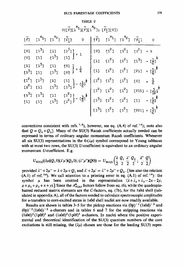
The 2,/~ dependence of the SU(3) dimensionality is given in connection with eq. (9); dimsv(,)[~ denotes the dimension of the SU(4) representation [_/7']. The U- coefficients are SU(3) and SU(4) Racah coefficients, 6-(2/~) or 6-[97] coefficients, again in unitary form, and are given in a notation which is a direct generalization of that for the angular momentum recoupling coefficient, U ( J I J 2 J J 3 ; J t 2 J 2 3 ). The SU(4) Racah coefficient of eq. (14) with the scalar representation [0] (= [14]) in the 23 position has a magnitude given by the simple SU(4) dimension ratio 17): [dim DT'~]/dim [1 ~] dim [_~]½. Some of the most useful values are shown in table 2. The numbers show that transfers of(ls0d) a (lp0f) ~ clusters in stripping reactions, for example, are inhibited by this recoupling coefficient, most strongly for nuclei with A = 4n + 1 (by a factor of ~) , somewhat less so for nuclei with A --- 4n + 2, 4n + 3, (by factors of 61 and s ~, respectively); but there is no such inhibiting factor for A = 4n nuclei. The SU(3) Racah coefficients are available through the code of Akiyama and Draayer 7). Algebraic expressions for these coefficients are also available through the work of Biedenharn et al. 22); [see eqs. (3.46) and (3.56) of ref. 22); for phase
SU(3) PARENTAGE COEFFICIENTS 379
TABLE 2
u([~][].xl][~B[].x2]; [f-i][o]) [~'] x I ~ [1 ] [].½] [q] u
[ 0 ] [13 ] [ i ] [13 ] l
J + 1
[o3 i f ] [ i 3 ] [z]
[1] [].3] [ i ] [o] +¼ [].3] [1] [13 ] to] J
[12 ] [1] [].3] [133
[ I ] [ I ] [].3] [12]
[~] [l xl] [z xe] [~{] u
[o] [12 ] [z 2 ] [z 2] + l
[1] [12 ] [12 ] [13 ] - ~]~-
[13 [12 ] [12 ] [21] + [~]½
1 []-23 [12 ] [12 ] to] +
[12] [].2] [].2] [21].] - [~5.~-] ½
[13 ] [ i 2 ] [ze] [ i ] - [~]½
[13 ] [].2] [12 ] [221] + [53½
conventions consistent with refs. 7,s), however, see eq. (A.4) of ref. ,4); note also that Q = Q1 +Q2]. Many of the SU(3) Racah coefficients actually needed can be expressed in terms of ordinary angular momentum Racah coefficients. Whenever all six SU(3) representations in the 6-(2#) symbol correspond to Young tableaux with at most two rows, the SU(3) U-coefficient is equivalent to an ordinary angular momentum U-coefficient. E.g.
Usu(a)((2#XQI°X2'#'XQ2°);(2"#"XQ°))= Usu(2) 2 2 2 ' 2
provided 2" + 2/~" = A+2/~+Qt and A ' + 2 / = 2 " + 2 # " + Q2. [See also the relation (A.1) of ref. 14). We call attention to a printing error in eq. (A.1) of ref. ,4): the symbol # has been omitted in the representation ( 2 + A 2 + A a - 2 x - 2 y , ~2 + ~2 "q- ~3 "~ X + y).] Since the ARLsj factors follow from eq. (6), while the quadruple- barred reduced matrix elements are the C-factors, eq. (7b), for the ls0d shell (tab- ulated in appendix A), all of the factors needed to calculate spectroscopic amplitudes for ~-transfers to core-excited states in 1 sOd shell nuclei are now readily available.
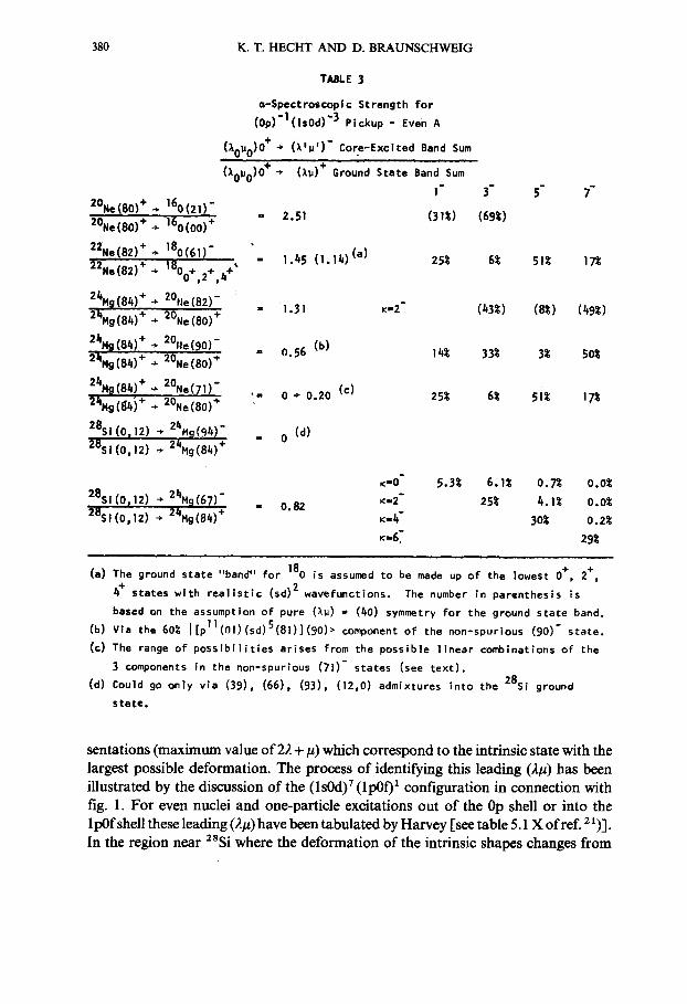
Results are shown in tables 3-5 for the pickup reactions via (0p)-1 (ls0d)-a and (0p)-2(ls0d) -2 ~t-clusters and in tables 6 and 7 for the stripping reactions via (lsOd) 3 (lpOf) 1 and (lsOd) 2 (lpOf) 2 ~-clusters. In nuclei where the positive experi- mental and theoretical identification of the SU(3) quantum numbers of the core excitations is still missing, the (2#) chosen are those for the leading SU(3) repre-
380 K . T . H E C H T A N D D. B R A U N S C H W E I G
20.e(80) + + 160(21)" 20Ne(80) + + 160(00) +
22Ne(82) + + 180(61 ) -
22Ne(82) + + 1800+,2+,4+"
24N~(84) + + 20fie(82 ) - =
24Hg(8~)+ + 2ONe(80) +
24H9(84) + + 20Ne(90)-
2kHg(84) + ÷ 20Ne(80)*
24Hg(84) + + 20Ne(71 ) " 2 k M g ( 8 4 ) * ÷ 20me(80) + "
28Si(0e12) 24H9(94)- (d) 8si(o,12) 2%(84) + - o
TABLE 3
o-Spectroscoplc Strength for (Op) ' l ( |sOd) "3 Pickup - Even A
(~OUo)O + + (~l~=)" Core.Excited Band Sum , q _ , , ,
(XOUo)O + * (X~)+ Ground State Band Sum
I"
= 2.51 (3 t t )
= 1.45 (1 .1~ ) (a)
5 " 5 "
(69~)
1.51
0.56 (b)
0 + 0.20 (c)
7
25t 6t 5It 17g
28Si(0pi2) + 2kH9(67 ) - 28Si(0,12) + 24Hg(84) +
= O. 82
K-2 (43t) (8~) (49t)
14~ 33~ 3t 50~
25t 6t 5it 17t
K=o" 5.3t 6.1~ o.7t o.o~ ~-2" 25t 4 . I t 0.Or x-4" 30~ 0.2 t
K-6~ 29t
(a) The ground state "band" for 180 is assumed to be made up of the lowest 0 +, 2 + , 4 + states wi th r e a l i s t i c (sd) 2 wavefunctions. The number in parenthesis is based on the assumption of pure (Z~) = (40) symmetry for the ground state band.
(b) Via the 60~ I [p l l (o1 ) (sd )5 (81) ] (90)> component of the non-spurious (90)" s ta te . (c) The range of p o s s i b i l i t i e s ar ises from the possible l i near combinations of the
3 components in the non-spurious (71)- states (see t ex t ) . (d) Could go only v ia (39), (66), (93), (12,0) admixtures in to the 28Si ground
s t a t e .
sentations (maximum value of 22 +/+) which correspond to the intrinsic state with the largest possible deformation. The process of identifying this leading (2/~) has been illustrated by the discussion of the (ls0d) 7 (lp0f) 1 configuration in connection with fig. 1. For even nuclei and one-particle excitations out of the 0p shell or into the 1 p0f shell these leading (2#) have been tabulated by Harvey [see table 5.1 X of ref. 21)]. In the region near 2sSi where the deformation of the intrinsic shapes changes from
SU(3) PARENTAGE COEFFICIENTS
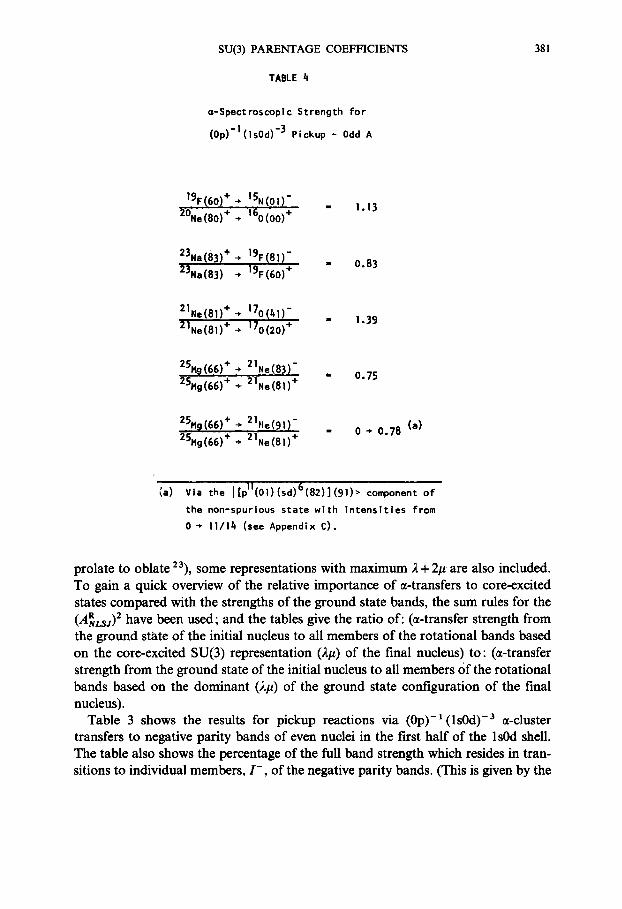
TABLE 4
a-Spectroscoplc Strength for
(Op)-l( lsOd) -3 Pickup - Odd A
381
19F(60) + ÷ 15N(Ol)- 2ONe(80) + ÷ 160(00) +
23Na(83) + ~ 19F(81)" 23Na(83) ÷ 19F(60) +
21Ne(81) + ÷ 170(41) - 21Ne(81) + ÷ 170(20) +
25M9(66) + ~ 21Ne(83)- 25Mg(66) + ÷ 21Ne(81) +
2 5 H 9 ( 6 6 ) + . 21t le(91)- 25Hg(66) + + 21Ne(81) +
1.13
= 0 .83
= 1 . 3 9
= 0.75
0 ÷ 0 .78 (a)
(a) Via the I [pll(01) (sd)6(82)] (91)> component o f
the non-spurlous state wi th i n t e n s i t i e s from
0 ÷ 11/14 (see Appendix C).
prolate to oblate 23), some representations with maximum 2 +2/~ are also included. To gain a quick overview of the relative importance of ~-transfers to core-excited states compared with the strengths of the ground state bands, the sum rules for the ( A ~ a ) 2 have been used; and the tables give the ratio of: (~-transfer strength from the ground state of the initial nucleus to all members of the rotational bands based on the core-excited SU(3) representation (2/0 of the final nucleus) to: (~-transfer strength from the ground state of the initial nucleus to all members Of the rotational bands based on the dominant (2/~) of the ground state configuration of the final nucleus).
Table 3 shows the results for pickup reactions via (0p)-l( ls0d) -a ~t-cluster transfers to negative parity bands of even nuclei in the first half of the ls0d shell. The table also shows the percentage of the full band strength which resides in tran- sitions to individual members, I - , of the negative parity bands. (This is given by the
382 K.T. HECHT AND D. BRAUNSCHWEIG
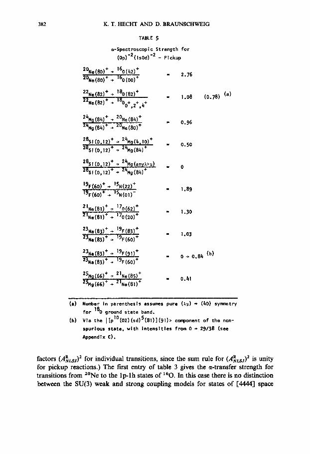
TABLE 5
~-Spectroscopic Strength fo r (Op)'2(IsOd) -2 - Pickup
2ONe(80) + ÷ 160(42) + 2ONe(e0) + + 160(00) +
2.76
22Ne(82) + ÷ ]80(82) +
22Ne(82) + ÷ 1800+,2+,4+ - 1 . 0 8 (0.78) (e)
24H~1(84)+ .+ 20He(84) + 24Mg(84) + ->. 2ONe(80) +
- 0 .96
28Sf(Oe12)+ + 24Hg(4elO)+ 28SI(0,12) + ÷ 24Hg(84) +
- 0 .50
28Sl(Or12) + + 24Hg(any~>#) . 28Si(0,12) + ÷ 24Hg(84) +
i9F(60) + + 15H(22) +
19F(60) + ÷ 15N(01)- 1.89
21Ne(81) + ÷ 170(62) + 21Ne(81) + ÷ 170(20) +
- i . 30
23Na(83) + + 19F(83)+ 23Na(83) + ÷ 19F(60) +
- 1 .03
~3Na(83)+ ÷ 1 9 F ( ~ 1 ) + - 0 + 0 . 8 4 (b )
23Na(83) + + 19F(60) +
25H9(66)~ ÷ 21Ne(85) + 25Mg(66) + ÷ 21Ne(8i) +
- 0 . 4 1
(a) Number In parenthesls assumes pure ( ~ ) - (40) symmetry for 180 ground state band.
(b) Via the I [p10(O2)(sd)5(81)](91)> component o f the non- spurious s ta te , wi th In tens i t i es from 0 + 29/38 (see Appendix C).
factors (ARLs~,) 2 for individual transitions, since the sum rule for (ARLsj) 2 is unity for pickup reactions.) The first entry of table 3 gives the ~-tramfer strength for transitions from 2°Ne to the lp-lh states of 160. In this case there is no distinction between the SU(3) weak and strong coupling models for states of [AaA.A] space
SU(3) PARENTAGE COEFFICIENTS 383
symmetry, since the state [(21#1)(22#2)](2#)= [(01)(20)](21) is the only non- spurious state of lhco excitation 14). With A~t. = 0.23 for 2°Ne(80) ~ x60(00); table 3 leads to the strengths A~t = (2.51)(0.31)(0.23) = 0.18 for the transition to the 1- state, and A~s = (2.51)(0.69)(0.23)= 0.40 for the 3- state. Since the 3- and 1- states at 6.13 and 7.12 MeV in 160 are not pure lp-lh states of [A.A.A.A.] sym- metry, these are overestimates. On the basis of the Ellis and Engeland to) wave functions for these states, the 3- state at 6.13 MeV is predicted to have a lp-lh content of 78 %, and only 72 % of this belongs to the S = 0 state of [A.A.A.~] symmetry so that A~3 would be reduced by a factor of 0.56 to a value ofA~s = 0.22. Similarly, the 1- state at 7.12 MeV has a lp-lh content o f71% of which 76% belongs to the S = 0 state of [A.A.A.A.] symmetry, so that A~I is reduced by a factor of 0.54 to A~I = 0.097. Assuming that the 3p-3h components can be approximated by the SU(3) strong coupling states [(03)(60)](63) of [A.A.AA.] symmetry the ~-spectroscopic amplitudes to the 3p-3h components of these states would be given by A~s = 0.002 and A~ 1 = 0.031. These spectroscopic amplitudes for a transfer with Q = 2N+ L = 5 (compared with Q = 7 for the ~-transfer to the dominant lp-lh pieces), must, how- ever, be multiplied by kinematic (reaction mechanism) factors which can be expected to be smaller by an order of magnitude compared with the Q = 7 kinematic factors. Even for the transfer to the 1 - state the coherent superposition of 3p-3h and lp-lh contributions should lead to no more than 10% corrections to the cross section, compared with the predictions based on the dominant lp-lh components alone.
The pickup reaction on 22Ne to the K = 1 - band in xao, approximated by the SU(3) strong-coupling state [(01)(60)](61), can again be expected to be strong compared with transitions to the lowest 0 +, 2 +, 4 + states in xso. In this case re- alistic 1sO wave functions s. 24) have been used to calculate the ~-particle spectro- scopic amplitudes to these 0 +, 2 +, and 4 + states. If on the other hand the wave func- tions for these states were approximated by states of pure (2p) = (40) symmetry, the predicted strength to this "rotational band" changes by only ~ 25 %, even though 180 is by no means a good SU(3) nucleus. [The weak coupling wave functions of Ellis and Engeland l O) indicate that the strong coupling approximation for the K = 1- band may be quite good.] The numbers for pickup transitions to 160 and i s o lead us to expect that estimates based on the SU(3) strong coupling model should be fairly reliable for heavier nuclei in the l s0d shell with well-developed negative parity rotational bands. With eq. (8) and the entries from table 1 of appendix A the numbers in table 3 can be converted to absolute values for the A2L. E.g., for the transition to the 1- state of the (61) band in 1so, A21 = 0.063, somewhat high compared with recent experimental results 2s) for the (d, 6Li) cross section to the 1 - state at 4.45 MeV in 1sO.
Table 3 shows the pickup strengths to three negative parity rotational bands in 2°Ne. The total ~-transfer strength to the K = 2- band based on the SU(3) strong coupling state [(01)(81)](82) which is identified with the experimentally observed 15) band at 4.97 MeV is larger than the summed strength to the (80) ground state ro-
384 K.T. HECHT AND D. BRAUNSCHWEIG
tational band by a factor of 1.31 and moreover is concentrated in just three states with a preference for the 3- and 7- states. The 0 + --, 0 + ground state to ground state transition, on the other hand, takes up only 21% of the total strength to the (80) band, [see table 3 of ref. 3)]. (Note that the K = 0- rotational band based on (2#) = (82), with r = 0-, 2-, 4 - , . . . , as well as the I = even members of the K = 2- band, have a predicted strength of zero.) The K = 0- band with/~ = 1-, . . . . 9-, and bandhead at 5.79 MeV is identified with (2p) = (90). It is built 1) from the two states: I[(0p) 11 (01) (ls0d) 5 (81)](90)) and I[ls0d) 3 (60) (113001 (30)](90)). One linear combination of these two states is the spurious state with 1 hco excitation in the c.m. motion (appendix C). The g-pickup strength shown in table 3 comes from the 60 (0p) 11 (1 s0d)S component of the non-spurious state. A third negative parity rotational band has been identified in 2°Ne with K ~ = 1-, and with bandhead at 8.72 MeV. There are three configurations with resultant (2p) = (71) which can give rise to such a band: I[(0p)lZ(01)(ls0d)5(81)](71)), [[(0p)Xl(01)(ls0d)5(62)](71)), and I[(1s0d)a(60)(lp0f)l(30)](71)). Note, however, that one linear combination of these three states is a spurious state with I hco excitation in the c.m. motion (appendix C). The remaining two (A/a) = (71) bands built from these three configurations are proper core-excited states in 2°Ne. The a-pickup strength depends on the relative amplitudes of the first two components. However, it is largest if the coefficient of the second, (ls0d)5(62), term is zero. In this case the coefficient of the I[(0p)11(01) (1s0d)S(81)](71)) component is [24/79] ~r. Since the (22/a2)= (81) states lie much lower in energy than the (62) states in the (ls0d) 5 nucleus 21Ne, we would expect this to be the best approximation for the 1- band at 8.7 MeV in 2°Ne and take the ratio 0.20 in table 3 as the best estimate for the a-pickup strength to this band. (The value 0.0 is obtained for a state for which the amplitudes of the three components above are 0.60, -0.70, and -0.38, respectively.) It should also be noted that the a-stripping strength to this band from 160 is zero even though it has a sizeable (ls0d) a (lp0f) 1 component. Since the transfer of a (ls0d) a (lp0f) 1 a-cluster carries an SU(3) representation (90), the transition is forbidden by the selection rule (00) x (90) ~, (71).
Table 4 shows the results for the pickup reactions via transfers of (0p)-1 (1 sOd)-3 a-clusters to negative parity rotational bands of odd-A nuclei, and table 5 the results for pickup reactions via transfers of (0p)-2 (1 sOd)-2 a-clusters to low-lying positive parity 2p-2h configurations for nuclei in the first half of the (ls0d) shell. Since the ARLsa factors can be calculated with available computer codes ~), the percentages of the summed strength in transitions to invividual states are not included. The tables show only the ratios of the summed pickup strength to all members of the rotational bands of the core-excited (g/a) relative to those to the ground state rotational band. In almost all cases the core-excited bands compete favorably with the ground state bands.
Stripping reactions via the transfer of ( l s 0 d ) a ( l p 0 f ) 1 a n d (ls0d)2(lp0f) 2 a- clusters may be particularly important. With a transfer of Q = 9 and 10, they are
SU(3) PARENTAGE COEFFICIENTS 385
TABLE 6
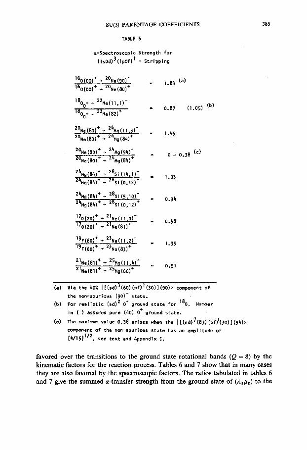
~-Spectroscopic Strength fo r (IsOd)3(lpOf) I - S t r ipp ing
160(00) + ÷ 2ONe(90 ) -
160(00) + ÷ 2ONe(80) + 1.83 (a)
1800+ + 22Ne(11,1)- . . . . . . 0.87 ( I .05) (b)
I~O0+ + 22Ne(82) +
2ONe(80)+ ÷ 24H9(1113)- - 1.45 2ONe(80) + + 24Hg(84) +
2ONe(80)+ ÷ 24H~(94)" - 0 + 0.38 (c) 2ONe(80) + ÷ 2~Hg(84) +
24H9(84)+ + 28St ( l%1) - 24Hg(84) + ÷ 28Si(0,12) +
24H9(84)+ ÷ 28Si(5,10)- 24Hg(84) + + 28Si(0,12) +
170(20) + ÷ 21Ne(11,O!~, ] 7 0 ( 2 0 ) + + 21Ne(81) +
19F(60) + ÷ 23Na( l l t2 ) " 19F(60) + ÷ 23Na(83) +
21Ne(81) + + 25H9(11 /,t ) - 21Ne(81) + ÷ 25Hg(66) +
- 1 . 0 3
= 0 . 9 4
= 0 . 5 8
= 1 . 3 5
= 0 .51
(a) Via the 40¢ I [ ( sd )3 (6O) (p f ) l (30 ) ] (90 ) > component of
the non-spurious (90)- s ta te . (b) For r e a l i s t i c (sd) 2 0 + ground s ta te fo r 180. Number
in ( ) assumes pure (40) 0 + ground s ta te .
(C) The maximum value 0.38 ar ises when the I [ (sd )7 (83) (p f~ (30) ] (94)> component of the non-spurious s ta te has an ampli tude of [4/15]1/2p see tex t and Appendix C.
favored over the transitions to the ground state rotational bands (Q = 8) by the kinematic factors for the reaction process. Tables 6 and 7 show that in many cases they are also favored by the spectroscopic factors. The ratios tabulated in tables 6 and 7 give the summed ~-transfer strength from the ground state of (2 0 Po) to the
3 8 6 K . T . H E C H T A N D D . B R A U N S C H W E I G
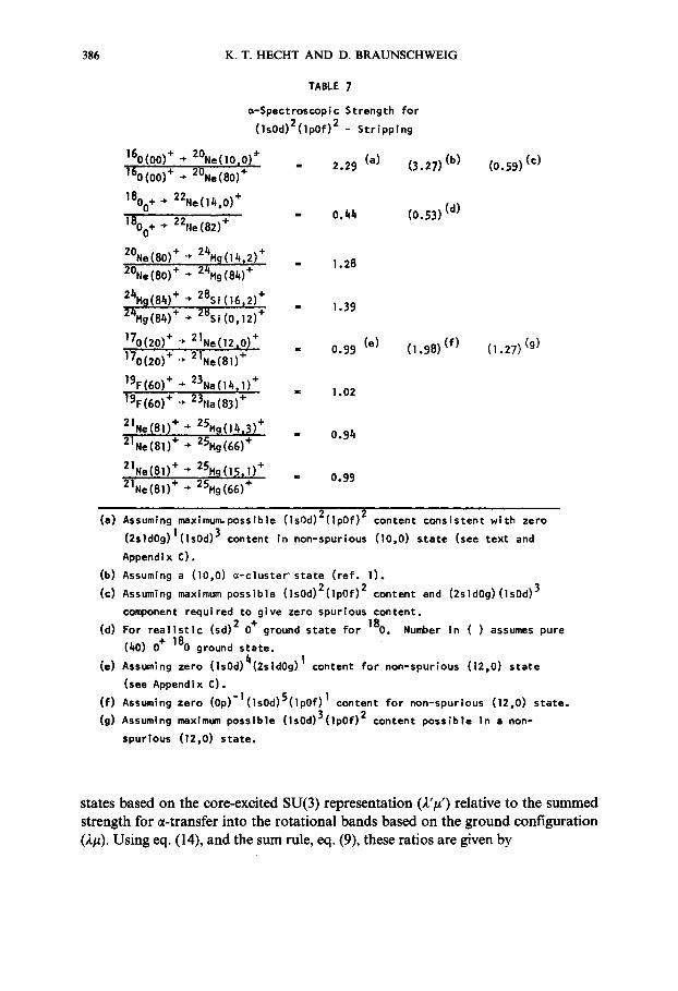
TABLE 7
~-Spectroscopic Strength for ( lsOd)2(lpOf) 2 - St r ipp ing
160(O0)+ ÷ 20Ne(10'O)÷ " 2.29 (a) (3.27)(b) 160(00) + ÷ 2ONe(80) +
]800+ ÷ 22Ne(14,0) + = 0.44 (0.53) (d)
18Oo. + 22.e(82)*
2ONe(80)+ + 24H~(14p2)+ = 1.28 2ONe(80) + + 24Hg(84) +
24H~(84)+ ÷ 28Si(16e2)+ - 1.39 24Hg(84)+ ÷ 2BS1(0,12)*
170(20)+ ÷ 21Ne(12=0)+ " 0.99 (e) (1.98) ( f ) 170(20) + ÷ 21Ne(81) +
19F(60) + + 23Na(1411) + = 1.02
]9F(60) + ÷ 23Na(83) +
21Ne(81)+ ÷ 25H~(14~3)+ - 0.94 2~Ne(8]) + ÷ 25Hg(66) +
21Ne(8]) + ÷ 25H9(15~1) + = 0.99
21Ne(81) + ÷ 25Hg(66) +
(0.59) (c)
(1.27) (g)
(a) Assuming maxlmum, possible ( isOd)2(IpOf) 2 content consistent wi th zero (2sldOg) l( IsOd) 3 content in non-spurious ( lO,0) s tate (see tex t and Appendix C).
(b) Assuming a (10,0) a-c luster" state ( re f . 1). (c) Assuming maximum possible (]sOd)2(lpOf) 2 content and (2sldOg)(isOd) 3
component required to give zero spurious content. (d) For r e a l i s t i c (sd) 2 0 + ground state for 180. Number in ( ) assumes pure
(40) 0 + 180 ground s ta te .
(e) Assuming zero (IsOd)4(2sldOg) 1 content fo r non-spurious (12,0) s ta te (see Appendix C).
( f ) Assuming zero (Op) ' l ( lsOd)5( ipOf) I content fo r non-spurious (12,0) s ta te . (g) Assuming maximum possible ( lsOd)3(lpOf) 2 content possib le in a non-
spurious (12,O) s ta te .
states based on the ~re-excited SU(3) representation (2'#') relative to the summed strength for or-transfer into the rotational bands based on the ground configuration (2#). Using eq. (14), and the sum rule, eq. (9), these ratios are given by
SU(3) PARENTAGE COEFFICIENTS 387
8-4X(,;.o/to ) --} By(A'/t') B-4X(Ao/to) ~ BY(A/t)
= ( B 2 (C[(ls0d) q]) 2 2 dim \ B - 4 J (6[( ls0d),])2 (C[(lsod),])2 Usu{3)Us2u{,, dim ' (:6)
where the SU(3) and SU(4) Racah or U-coefficients are those defined by eq. (14). Since both low-lying K s = 3- and 0- bands are known in 2*Mg, table 6 gives the
~-transfer strength for stripping into bands based not only on the I[(ls0d)7(83) (1 p0f) ~ (30)](11,3)) state corresponding to maximum possible intrinsic deformation, but also to bands based on the lower SU(3) representation (k/t)= (94) since it contains a K = 0- band. The SU(3) strong-coupling state 1[(83)(30)'1(10,2)) is not included since g-transfer from the major (80) component of the ground state of 2°Ne to this state is forbidden by the selection rule (80)x (90)÷ (10,2). Moreover the K = 0- band of this representation leads to P = 0- , 2- , 4 - , . . . only. Although the summed strength into the bands based on (11,3) is large, th0 I - = 3-, 5-, 7-, 9- members of the K = 3 band take up only 0.06, 1.5, 9.9, and 30.3 ~ , respectively, of this summed strength, while the 1-, 3-, 5-, 7-, 9- members of the K-- 1 band take up 5.5, 21.4, 19.7, 2.0, and 9.7~o of this strength. Since there are three con- figurations of 1 hco core excitation with (A/t) = (94) and one spurious component (see appendix C), the two non-spurious states with (~./t) = (94) must be linear com- binations of the three states I[(0p)lX(01)(ls0d)9(93)](94)), I[(ls0d)~(83) (lp0f)~(30).1(94)), and I[(ls0d)7(64)(lp0f)t(30).1(94)), and the ~-transfer strength depends on a coherent superposition arising from the last two components and can vary from zero to a maximum which leads to the ratio of 0.38 of table 6. The 1 -, 3- , 5-, 7- , and 9- members of the K = 0- band of (94) take up only 22.7, 4.9, 0.6, 3.8, and 0.2 %, respectively, of the summed strength.
The stripping into the (10,0) band of 20Ne via an ( 1 s0d)2( 1 p0f)2 cluster may hold partic- ular interest. It has been suggested ~ 5) that a K = 0 + band with band head centered on the wide level at 8.3 MeV, may be a band based on the (ls0d) 2 (lp0f) 2 configuration. The calculations of Strottman and Arima 12) seem to confirm this possibility. There are, however, seven ways of constructing SU(3) strong coupling states with an ex- citation of 2hco, coupled to (k/t) = (10,0). Only one of these is based on the con- figuration (ls0d)2(lp0f) 2, a second on the configuration (ls0d) 3 (2sld0g) 1, while the remaining five involve excitations out of the 0p shell (see appendix C). Two of the seven states with (k/t)= (10,0) are spurious, corresponding to excitations of 2hr~ and 1 hco of the c.m. motion, respectively, where the 1 ho~ excitation is based on the non-spurious (90) state. The spurious states are constructed in appendix C. If it is assumed that the lowest non-spurious state with (A/t) -- (10,0) has zero (2sld0g) content, but maximum possible (ls0d) 2 (lp0f) 2 content consistent with this assump- tion, the amplitude of the I[(ls0d)2(40)(lp0f)2(60)](10,0)) component of the non-spurious state is only a = 0.517, but leads to the ratio 2.29 of table 7. If, on the
388 K . T . HECHT AND D. BRAUNSCHWEIG
other hand, it is assumed that the lowest non-spurious (10,0) state has maximum possible (ls0d)2(lp0f) 2 content, then the requirement that the state have zero spurious content leads to amplitudes of a = [~o] ½ = 0.608 and b = - 21/[ 1850] ½ = -0.488 for the I[(ls0d)2(40)(lp0f)2(60)](10,0)) and t[(ls0d)3(60)(2sld0g) 1 (40)](10,0)) components. In this case the two components will interfere destructively in their contribution to the ~t-transfer strength, leading to the ratio 0.59 of table 7. It is interesting to note that the (10,0) "cluster state" constructed by Ichimura et al. 1) has coefficients a = [ ~ x a~] ½, b = [ ~ x ~]½, leading to constructive inter- ference for the ~-transfer and a ratio of 3.27 in table 7.
Although accurate predictions for ~-spectroscopic amplitudes to any specific core excited state in an s-d shell nucleus will undoubtedly require more detailed structure calculations taking into account the effects of representation mixing, the numbers of tables 3-7 can be used as a zeroth order guide for the or-transfer strengths. They also show that ~-transfer amplitudes to core-excited states are generally as large as those for bands based on the ground state configuration.
Appendix A
FEW-NUCLEON PARENTAGE COEFFICIENTS
The ready availability of the SU(3)/R(3) parts of the n --, ( n - x ) nucleon parentage coefficients through the code of Akiyama and Draayer 7) has reduced the parentage problem to the calculation of the SU(6)/SU(3) parts of these coefficients. Although these could be generated by a recursive process from one- and two-nucleon c.f.p., it is simpler to calculate the x-nucleon reduced matrix elements directly, particularly for the physically most interesting states with large values of 22 + # (alternately 2 + 2#). Since only the SU(6)/SU(3) factors of the reduced matrix elements are needed, it is simplest to extract these from the full matrix elements calculated in the [SU(4) x SU(6) ~ SU(3) D [SU(2) x U(1)]] scheme, using the Elliott 21)intrinsic
oscillator quantum numbers, e A M A ; where the SU(2) representations are charac- terized by the A-spin, while U 1 is characterized by e = ~ ( 2 n z - n x - n y ), see fig. 1. In the ls0d shell the single-particle SU(2) x U(1) quantum numbers have the simple values~ A = 0, e = 4; A = ½, e = 1 ; A = 1, e = - 2 . The spectroscopy is therefore one involving the coupling of a small number of particles of small A-spin with real spin ½ and isospin ½ in configurations to be denoted by:
;12 n 3 (A = 0, e = 4)~},j,t,(A = ½, e = 1)t721A2(A = 1, e = --2)[~3]A 3.
The coupling problems associated with this spectroscopy will be illustrated in some detail for the seven-particle system, by the most important states for the spectrum of 23Na, in particular. The seven-particle (1 sOd) configuration with largest possible e (5 = 19; nl = 4, n2 = 3, n3 = 0) is illustrated as part of the configuration of fig. 1. The four identical (A = 0, e = 4) particles can couple only to the totally
SU(3) P A R E N T A G E C O E F F I C I E N T S 389
antisymmetric SU(4) representation [_)7'1] = [14] = [0], the scalar representation of SU(4) with S = 0, T = 0, or ( P P ' t v ' ) = (000) in terms of Wigner's supermultiplet labels 17). The three identical (A = ½, e = 1) particles can couple only to total A- spin of 2 a for the totally antisymmetric supermultiplet [1 a], with ( P P ' P " ) = 1 1 (2 • -½), or to total A-spin of ½ for the SU(4) representation [211, with ( P t V P '') = ta_ ± xx 1,2 2 21"
With Ma = A these states, with maximum possible e for the configuration, cor- respond to SU(3) highest weight 21) states with e = 2 2 + # and # = 2Ma; hence (2/0 = (83) for the supermultiplet [13], or space symmetry [43], and (2t~) = (91) for the supermultiplet [21], or space symmetry [421]. With e = 16, there are two
4 possible configurations (A = 0, e = 4)7131o (A = ½, e = 1)0,2]a2 with [_~21A 2 = [1412, [21111, or [22]0; and (A = 0, e = 4)~*o] o (A = ½, e = 1)~,2]a2 (A = 1, e = -2)dl]1, now with [.~2]A2 = [1211, or [2]0. Simple SU(4) and A-spin coupling leads to the enumeration of the possible coupled final [.)7] and total A-spin values for these two configurations. To illustrate with a specific example, states with a final [J~] = [131, corresponding to highest possible space symmetry [43], can be constructed only from [(A = 0, e = 4)7131o (A = ½, ~ = 1)~1412] ; [(A = 0, e = 4)71,10 (A = ½, e = 1)~21111] ; and [(A = 0, ~ = 4)~1,]o (A = ½, e = 1)71211 (a = 1, e = -2)d1111; with total A-spins of 2; 1 ; and 0, 1,2. Of these five states with space symmetry [43] and ~ = 16, two (with A-spins of 1 and 2) belong to the (2#) -- (83) representation whose highest weight e is 19. The remaining three (with A = 0, 1, 2) give rise to new intrinsic states of highest weight in SU(3) with 22+/~ = 16 and # = 2A, hence (2/~) = (80), (72), (64). Continuing the process, there are three possible configurations with ~ = 13: ( A = 0 , e=4)~1~]o ( A - 1 = 1 5 = - ~ , e )tJ'21a2, with [_J?2]A2 [213]~2, or [2211½; ( A = 0 , e = 4)7131o (A = ½, ~ = 1)Oi~]a~ (A = 1, e = -2)~1] 1 , with [.]'2]A2 = [131~ or [21]½;
2.. and (A = 0, ~ = 4)~'1,]0 (A = ½, 8 = 1)~1] ½ (A = 1, 8 = -2)[i3]a3, with [_)7'3]A 3 = [1210, [1212, or [211. Again, restricting the discussion to states with [ .~ = [13], cor- responding to space-symmetry [43], there are now six ways of coupling [-~1] [~2] [~3] to resultant [ .~ of [13], with total A-spins of { (5 occurences), 2 a (5 occurences), and 2 ~ (3 occurences). Of these 13 states with e = 13, three (with A = _12, a2, ~) belong to (2/~) = (83), one (with A = ½) to (80), two (with A = ½, a) to (72), and two (with a 3 5 = ~, ~) to (64); leaving five ~ = 13 states (with A = ½, _12, _32, ~2, z~2j which become highest weight states in new SU(3) representations with 22 + # = 13; that is, two independent states with (2/~) = (61), two independent states with (2/~) = (53), and one with (2/0 = (45).
To find the proper linear combinations of the full set of states which are of highest weight with respect to both SU(3) and SU(4), a computer code has been constructed. First, all states of the proper e M a M s M r Y are constructed in the occupation number representation for this scheme, with e, M a . . . set equal to e = 22+#, Ma = ½bt, and M s = P, M r = P' , Y = P " , the desired highest weight quantum numbers for SU(3) and SU(4), respectively. [The SU(4) quantum numbers are here given in terms of Wigner's supermultiplet labels P P ' P " ; Y is the third additive quantum number for SU(4), the eigenvalue of Eoo in the notation of ref. 17). 1
390 K . T . H E C H T A N D D. B R A U N S C H W E I G
Next, the highest weight states are constructed by simple step-up operator arithmetic. The proper linear combinations of states of the appropriate eAMAMsM r Y must yield zero when acted on by the SU(3) step-up operators Az~, A~y, A~y = A+, and by the SU(4) step-up operators S+, T+, El l , Elo, Eo~, E~_ 1 [in the notation of refs. 21. t 7), respectively].
It is sufficient to calculate the matrix element of the x-nucleon creation operators between n and ( n - x ) nucleon states which are of highest weight with respect to both SU(3) and SU(4), since both the SU(3)/R(3) and SU(3)/[SU(2) × U(1)], as well as the SU(4)/spin-isospin factors of these matrix elements are known. Lower weight states are therefore needed only for the x-nucleon creation operators, coupled to [-f~](,~x#x). For x = 1, 2, 3, 4, these have been constructed explicitly for all possible ~AMa SMs TMr by simple step-down operator arithmetic, again in the occupation number representation. The full matrix element of the x-nucleon creation operators then follows from a direct calculation of the overlaps of the occupied states.
Finally, the full matrix element of the x-nucleon creation operator is factored
((lsOd),[f,j~t,(2,#,)FA,M,a; R'~"Aar' T' ~,f' h, ttSxl(~x,,,) I-" ~ ~ ' A S .t z , ~ T I , ~ S x M S x T ~ M T x e x A x M A x
x [(lsOd)'-~[f]ctt2#)eAMa; flSM s T M r )
= ~ <[f']a'(2'#')ll Ilz*t~'~¢x~"x)°ll IIl-f]~(2#)><(X#)eZ; O.x#~)e~Z~ll(R'#')e'a'>p P
× [L]S x <SMsS~MsxIS'M's>(TMr T~MrJT'M'r>. (A.1)
The quadruple-barred matrix element of X* is the desired SU(6)/SU(3) factor of the reduced matrix element, the C-factor of eq. (7). Four bars are used to indicate that not only the dependence on all M-quantum numbers but also the dependence on SU(3) and SU(4) subgroup labels has been factored out of the full matrix element. The ( 1} ) factor is the reduced SU(4) ~ [SUs(2) x SUr(2)] Wigner coefficient, the D-factor of eq. (7), which for most cases of interest is available through the work of ref. 17). The M-dependent factors are ordinary angular momentum Wigner coef- ficients. The double-barred coefficient is a reduced SU(3) Wigner coefficient in the SU(3) ~ [SU(2) x U(1)] scheme which is available through the code of ref. 7). The SU(3) multiplicity label p is needed only for those (2x#x) for which the coupling (2#) x (2x#x) contains the coupled representation (2"K) with a multiplicity d, with d > 1. For the states of primary interest in this investigation, with [fx] = Ix], (2~#x) = (Q0)= (2x, 0), the SU(3) product (2#)x (Q0) is free of multiplicity; the label p is not needed, and the summation over p is replaced by a single term. To calculate the quadruple-barred reduced matrix element it is sufficient to choose highest weight states with respect to SU(3) and SU(4) for the n and ( n - x ) nucleon states in the full matrix element, that is to set e = 22 + #, A = M a = ½/~; S = M s = P, T = Mr = P', and to replace the SU(4) label fl by the highest weight value for
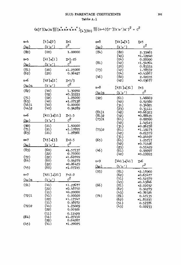
SU(3) PARENTAGE COEFFICIENTS 391
Table A. I
<~[f.l(x~)= IIll [J. £~ J- -+ ][4](8o) II1 (n-4) If' ](k 'I~' )0,' >2 = C 2
~--4 [4 %<0 ] ~-1 n--8 [44 ]-~4 ] (~) (~'~') c 2 (~) (~. ,)
(8o) (00) 1.0oo0o (84) (8o) (42)
n:5 [41 ].-,[i ] ~- i . 25 (04) (,~) (x ' . ' ) 02 (81) (42)
(20) (81) (20) .1. 25000 (73) (42) (62) (20) 0.96427 (04)
(46) (80) n=6 [42 ]..[2 ] ~-5/3 (42) ( ~ ) a (~'~') c 2
n=8 [431 ]-*[31 ] (82) (40) I . 3095O
(02) *0. 33333 (%~)~ (k ' . ' ) (71) (02) i . 25000 (92) (61) (63 ) ( 40 ) .1.07138 (42) (44)1 (40) 0.00000 (31) (44) 2 (40) O. 94289 (23)
(81)1 (42) n:6 [411~[11] ~1.5 (8].)2 (42) LkB) (X ' . ' ) C 2 (73)1 (61)
(42) (90) (21) i . 50000 (31) (71) (21) -1.17855 (73)2 (61) (63) (21) 1.28:.556 (42)
(31) n=7 [43]-[3] ~-2.5 (65) (61) (~) (x ' . ' ) c 2 (42)
(23) (83) (60) *I. 57137 (46) (61)
(22) o. 75ooo (42) (72) (22) -1.60709 (6 4) (6 O) O. 94279 n:9 [441 ]-,,[41 ]
(22) *o. 06429 ( 45 ) (60) *1.07145 (k~) (k ' . ' )
(93) (81) n:7 [421]-[21] 7=2.0 (62) (k,)a ( k ' . ' ) C 2 (51)
(43) (91) (bl) *1.27677 (66) (81)
(22) .0.48750 (62) ( l l ) *0. 20000 (43)
(72)1 (41) O. 00000 (74) (81) (22) *1.17547 (62) (ii) 0.38572 (51)
(72)2 (41) 1.25009 (43) (22) O. 00306 ( 11 ) O. 11429
(6 4) ( 41 ) * 1.0711~0 (22) 0.64287
(45) (41) *I. 20025
Z=-5 C 2
2. 33465 *i. 12240 O. 2OOOO
-1. 54764 O. 83333 i. 78572
*0.4166 7 2. 02035
*0. 03677
2=3 C 2
1.46669 o. 52380 O. 34921 O. 31111
*0.66323 *0.88435 O. 00000 i. 42123
*0.26 238 * l . 19173 O. 01579
*0.24497 1.25717
.o. 71426 O. 51429 o. 99997
*0.19993
~6 c 2
*2.18900 *0.65477 *o. 52379 *0. 43846 -2. 02032 O. 94279
*o. 76526 O. 47135
*i. 83335 0.52376 o. o2233
n=9 (~) (lO,1)
(74)
n=lO
(lO,2)
(83)
(75)
(56)
(48)
n=lO
(83)
(75)
(56)
[432 ].-*[32 ] (x'.')
(62) (51) (43) (62) (51) (43)
[442 ]~[42 ] (x ' . ' )~ ' (82) (63) (71) (6o)1 (60)2 (52) (44)1 (44)2 (82) (63) (71) (60)1 (60)2 (52) (44)1 (44)2 (82) (63) (71) (52) (44)1 (44)2 (82) (63) (71) (52) (44)1 (44)2 (82) (63) (44)1 (44)2
[4411]-~[411 ] (x'~')=' (71) (63) (52)1 (52)2 (90) (71) (63) (52)1 (52)2 (9O) (71) (63) (52)1 (52)2
~--3.75 c 2
-1.66672 *0. 30476, .0. 71426 *i. 09990 O. 78564 0.0
~7.5
c 2
2. 31533 0.84657 O. 35736 o. 19O47
*0.0846 5 O. 45917 O. %074 O. 05497
*0.64275 i . 01848 o. 08466
*0.%262 *0. 21936 .0. 32740 O. 00000 O. 72754 1. 92855 0.00000
*i. 10200 O. 21043 O. 2%73
*0.73048 *0. 35709 1.63328
.0. 05442 *0.61225 *0. 05454 *0. 57724 2. 35711
*i. 49995 o. 81818 O. 12462
Y'=7 C 2
O. 83808 i. 95554 O. 10576
.0. 06448 i. 45908
*0. 08978 *i .65012 O. 40792
*0. 2486 3 0.67345
*I. 34685 0.64002 O. 49452 O. 48994
n=ll
(z1,1)
(1o, o) (92)
(84)
(57)
(2,1o)
(38)
n=ll
(1o, o) (92)
(84)
(57)
n=12
(12,0)
(93)
(66)
(39)
(o,12)
[4~3 ]-~[43 ] (~'~')
(83) (72) (64) (64) (83) (72) (64) (83) (80) (72) (64) (83) (72) (64) (83) (64) (83) (64) (45)
[N421 ]-..,[421 ]
(~'.')c~' (64) (72)1 (72)2 (64) (91) (8o) (72)1 (72)2 (64) (91) (72)1 (72)2 (64)
[444 ]~[44 ] <x'~') (84) (73) (84) (81) (73)
(84) (81) (73) (46) (84) (73) (46) (84)
~=-i0 C 2
*2.87032 *0.88435 *i. 10386 2. 58580 O. 58437
*0. 02380 *I. 26270 -2. 14295 O. 77822 O. 3%79
*0.06667 *2. 20974 1. 47320 o. 076 71
*3. 75000 2. 25000 O. 31248
*i. 94875 O. 53322
}7=8.75 c 2
2. i0100 *0.14965 *0. 89781 *i. 77769 *i. 32645 O. 03537 o. 96216 O. 02567 i. o6688 1.57138 0.67347
*o. 11224 *i. 22722
E=I5 c 2
4. 89103 2.17379 2.80213
*I. 09449 *0. 07535 *0. 88309 2. 48672
*0.67344 *0. 94193 .0.68404 3. 39966
*2. 22527 *i. 07148 9.00000

SU(3) PARENTAGE COEFFICIENTS 393
*'*--12
(lO,1)
(93)
(66)
(39)
(1,1o)
n=12
(66)
n=13
(10,2)
(83)
(75)
(48)
(z ,n )
(o, io)
(29)
[4431]-~[431]
(73)1 (73)2 (65) (92) (81)1 (81)2 (73)1 (73)2 (65) (46) (92) (81)1 (81)2 (73)1 (73)2 (65)
(92) (73)1 (73)2 (65) (92) (73)1 (73)2 (65)
[4422 ]~[422 ] (~ ' . ' ) (lO, O) (81) (73)
[4441]~[~41] (~ ' . ' ) (93) (74) (66) (93) (7~) (66) (93) (74) (66) (93) (74) (66) (93) (74) (66) (74) (66) (93) (74) (66)
Z=35/3 n=13 c 2 ,(~)
0.07916 (83) 1.13981 (75) 2.19810 1.32652 (48)
*0.36483 o.ooooo (o,1o)
-1.16618 (29) *0.07b64 "1.13337 0.68686 n=14
.1.49656 *0.67344 (X'H") 0.22448 (i0,0) O.O6997 (84) 0.04976 1.12212 0.00000 2.29168 1. 37755 (65)
*0.02721 -1.37490 1.66667 2.18182
"1.55155 (57) 0.93333
~i0.5 C 2
1.16726 (2,10) *o.o6734 "1.95916
~=17.5 C 2 (38)
-1.47185 1.68215 2.28251
*0.76916 0.00000 n=l~ "1.77529 1.61173 (kF) *0.47616 -1.28391 (92) *2.26645 0.00000 (73) i. 35396 (65) 5.00000 2.50000
*2.50000 *2.50000 0.11665 1.12181
*0.66667 1.79483
[4432]-~[432] E=14 (~,.,) q2 (74) *0.33333 (lO,1) *1.o6399 (74) 1.14276 ( i0 , i ) -1.64994 (74) 1.78570 (74) *2.16667 (i0,I) "1.83333 (74) o.ooooo
[~-h42]~[442] ~=-21 (~,.,) c 2
(75) *2.74738 (10,2) 1.04758 (83) -1.14297 (75) .0.99625 (%) 1.41324
(10,2) *i.00729 (83) 0.19049 (75) *0.14385 (56) 0.08978 (48) 1.63045 (10,2) 1.63183 (83) *0.14732 (75) -1.58243 (56) 0.11688 (48) o.934o6 (o, io) *0.53966 (lO,2) 3.66667 (83) 1.50000 (75) *2.37357 (56) -1.19043 (48) 1.33333 (10,2) 1.58078 (83). *0.33333 (75) 0.21151~ (56) 0.22222 (48) "1.53853
[44411]-~4411] ~2o (~,~,) o 2
(83) 1.o286o (75) 2.09236 (83) .1.4624o (75) 0.14544 (83) *0.13333 (75) *2.41678
*'denotes negative value for C.
394 K.T. HECHT AND D. BRAUNSCHWEIG
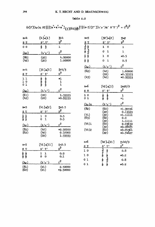
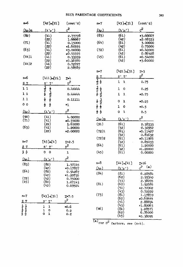
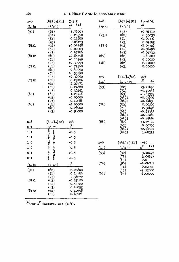
Table A.2
_ + + +. (nrr](x,): sTlll[a ,a -a ] [3](6O1_2L~..I I l(n-3)[f' ](~.',')c~' S'T') 2 = 02]) 2
n=1;
ST
O0
(~) (1;2)
n=1;
ST
ii
i0 Ol
(~)
(61) (1;2)
n=5
ST
[4 ] ~ [ i ] I)=1; n=5 [32 ]--,[2 ] ~--2 S' T' D 2 S T S' T' D 2 ,I
1 1 ~½ l O 1 ~ 1 2
(~.',') c 2 ½ ~'2 o 1 1 i I
(20) 1;.ooooo ~ ~ 1 o *0.5 (20) 1.~oooo ½ ½ o 1 o.5
(x~) (x ' , ' ) o2 [31]-,[1] ~1;/3 (62) (ho) 1.6oooo s' T' D 2 (02) *0.33333
# . i (1;3) (40) *0.93333
1 n=6 [I;2 ]-~3 ] ~--'-20/9 (x'~,') c 2 s T s' T' D 2 (20) 1.33333 10 i z 1 (20) *0.93333 o i
(x~)(~ (;,'~') 02
[1;J_],[2] ~2 .5 (82) (6o) .1.955~6 S' T' D 2 (22) 0.13333
(71) (22) .1.11111 (63) (6o) o.o
(22) l . 11111 (1;1;)1 (60) 2.03639
(22) *0. o81;85 (41;)2 (60) .0.01;361;
(22) .0.5h627
~ i 0 0.5 0 1 0.5
.(xH) (~'~,') c 2
(8].) (4o) *2.50000 (62) (ho) 0.10000
(02) Z. 33333
n=6 n=5 [41]~11] ~=2.5 s T S T S' T' D 2
i0 ½½ i i 0.9
IO O 0 0.I
Ol (~) (x'~,') c 2
O 1 (81) (21) 2.5000o (62) (21) *2.5000o
[he ]-,[21 ] s=4o/9 S' T' D 2
3 ! 0.8 2 s 1 I ~ *O.2
½ .~ 0.8 2 ½ ½ .0.2
SU(3) PARENTAGE COEFFICIENTS 395
(x~)a (82)
(71)
(63)
(~)1
(44)2
n=6
.ST
ii
ii
ii
O0
(9o) (n)
(63)
n:7 ST ½½ (~ )
(83)
(6~)
(72) (45)
n=7 ,S, T ! !
2 2
[42]421]
Ix'~') (41)
(41) (2~) (41) (22) (~1) (22) (41) (22)
[411~21] 8' T'
2~
2 ½½
I ½= (x"~') (41) (41) (22) (41) (22)
[43 ]~[4]
S' T'
00
(X'~')
(8o) (42) (8o) (~2) (~2) (8o) (t,2)
[43]-~[31]
8' T'
1 1 10 O 1
(cont' d) n=7 [43 ]~[31 ]
c 2 (~) (x'~,')
2.77778 (83) (61) 1.66667 (42) 0.15000 (64) (61)
-1.60555 (4~) .3.00000 (72) (61) .0.55555 (42) O. 33939 (45) (61)
~ . 16970 (42) O. 72727 2.58589
(eont'd)
C 2
*3.66667 .2. 08333 3.0O000 0.7500o
~o. 4o0oo o. 86428
.o. 54ooo "3.6o00o
n=7 [421 ]~[31 ] }~=3
~--4 S T S' T' D 2
D2 3½2 Z i 0.75
0.44~4 3 ½ i 0 0.25 2 o.4~44 ½ ~ z z .o.75 2 o.11111 ½ 3 o i ~.25
2 -i ½½ z o ~o.~
c 2 ½½ o i 0.5
4. O00OO c 2 ~ . 55000 (~)~ (X'~ ' ) i. 65000 (91) (6 I) 2.38333 1.200OO (42) O. 30952
*2. OOOO0 (72) 1 (61 ) .O. 11427 (42) o. 81632
(72)2 (61) ~.119o5 ~ 2 , 5 (42) o.85o33 D2 (64) (61) 1.200o0
( 42 ) * i . 20000 1 (55) (61) 0.00000
C 2
i . 57145 n=8 [44~[41] ~=-16 *0.17857 (k~) (k'g') C 2 (a)
O. 94287 (84) (81) 6. 28584 * i . 20716 (62) 2. 93340 O. 75000 (~3) 2.38095 1.07143 (81) (6_9) i. 92585 o. o9524 (5 z ) *2.709o2
(43) O. 72222 2-7.5 (73) (81) i . 17859
(62) .0.69444 D 2 (51) 2.88894
(43) "1.80063 ,0.6 (~ ) (81) 1.28571 o. 2 (62) 6.7600o O. 2 (43) *O. 38095
(a)For D 2 factors, see (n-4).
396 K. T. HECHT A N D D. BRAUNSCHWEIG
n:8 [431]-~41] (~)~ (x'~')
(92) (81) (62) (51) (43)
(81)1 (62) (51) (43)
(81)2 (62) (51) (43)
(73)1 (81) (62) (51) (43)
(73)2 (81) (62) (sz) (43)
(65) (81) (62) (43)
(h6) (81) (62) (43)
Z=-3.2 n=8 c 2 (a) (~)a
z.76oo3 0.25350 (73)1 0.1158O 0.06173
.O.64198 (73)2 0.00903 0.47186 .0.85598 (65) *0.14749 *0.32099 (46) .0.72960 0.42990
*0.35598 *0.30990 n=9 0.29184 1.28471 (XF) 0.24880 (93) 0.30291 1.25716
.O.8000O 0.10286
.1.ooooo (74) 0.28000
*0.96000
n=8 [431 ]4[32 ] ~,-4 8 T S' T' D 2
I i ~ ~ *0.5 2
1 1 ½ ,,0.5 l O ~ 2 .0.5
2 ~ 1o ½ ½ 0.5 o1 ½ 3 . o . 5 2 O 1 z i ~ *0.5
(~)~ (x ~ ' ) c 2
(92) (62) 2.02800 (51) o. 14486 (43) i. 38272
(81)1 (62) .0.32100 (51) 0.55320 (43) O. 44022
(81)2 (62) 0.10698 (51) O. 45526
(66)
n=9 (~)
(93)
(74)
(66)
[43114132] (x'~')
(43) (62) (51) (43) (62) (51) (43) (62) (43) (62) (43)
(cont'd) C 2
*O.91712 O.55030
,1.o2436 0.82542
-1.O3326 .o.%498 *0.05732 1.60000 0.00OOO 2.24000 0.00000
[44114142] ~9 (x'~')~' ~ (a)
(82) -3.21430 (71) *0.19048 (63) -1,83333 (44)1 *0.94696 (44)2 .o.1443o (82) o.ooooo (71) 2.30476 (63) *0.93333 (44)1 .o.OIO~O (44)2 *0.49496 (82) *3.77142 (63) 0.00000 (44)1 *0.54545 (44)2 1.68312
[441~[411] ~1o ,(x,~,) c 2 (a)
(90) 3.40477 (71) 2.09523 (63) o.o (9o) .~.o4~2 (71) 0.20952 (63) *2.52000 (63) 6.00000
(a)For D 2 f a c t o r s , see (n-4) .
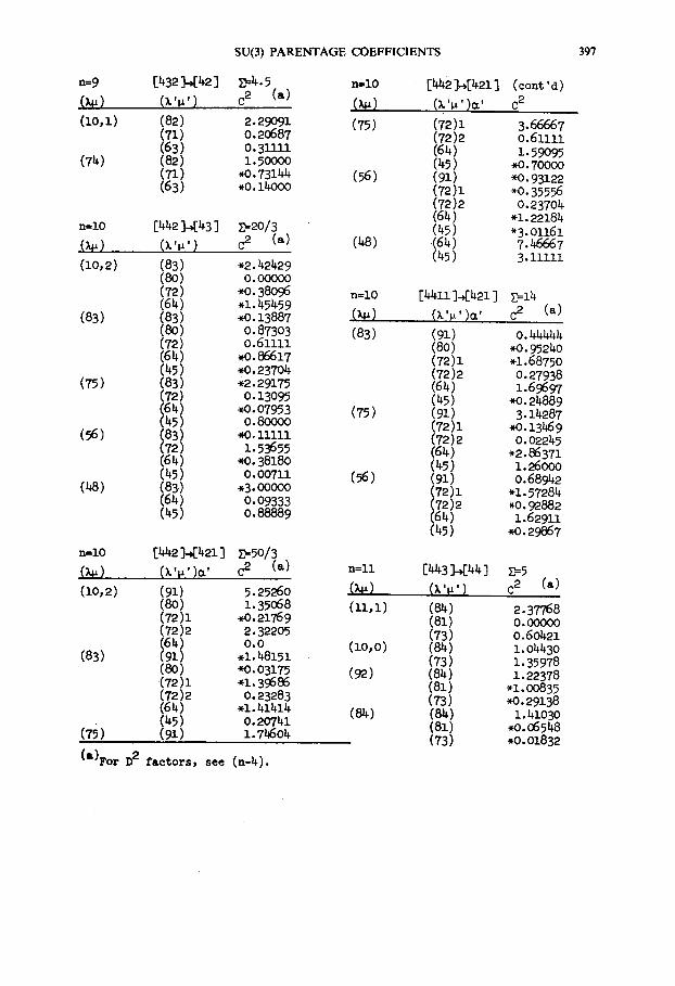
SU(3) PARENTAGE COEFFICIENTS 397
n:9 [432]-<42] ~:4.5 n=lO (~) (x ' . ' ) c 2 (~) (~)
(i0,i) (82) 2.29091 (75) (71) 0.20687 (63) 0.31111
(74) (82) 1.50000 (71) .0.73144 (56) (63) .0.14000
n=lO [442 ]--~[43 ]
(lO,2) (83) (8O) (72) (64)
(83) (83) (8o) (72) (64) (45)
(75) (83) (72) (64) (45)
(56) (83) (72) (64) (45)
(48) (83) (64) (45)
n = l O [442]-~421] (~) (x'~')='
(10,2) (91) (80) (72)1 (72)2 (6~)
(83) (91) (8o) (72)1 (72)2 (64) (45)
(75) (91)
~--20/3 C 2 (m) (48)
*2. 42429 0.00000
*0.38096 n=lO *i. 45459 *0.13887 ()4') O. 87303 (83) 0.61111
.0.86617 *0. 23704 *2. 29175 O. 13O95
*0.07953 (75) 0.80000
.0, iiiii 1.53655
*0.38180 o.ooTn (%)
-3.00000 O. O9333 O.88889
~5o/3 C 2 (a) n=l l
5.2526o (~) 1.35o68 (11,1)
*0.21769 2.32205 o.o (1o, o)
.1.48151 *0.03175 (92) -1.39686 o.23283
,1.41414 (8~) 0.20741 1.74604
(&)For D 2 factors, see (n-4).
[442 ~[421 ] (x ' , ' )= '
(72)1 (72)2 (64) (45) (91) (72)1 (72)2 (64) (45) <64) (45)
(cont'd) C 2
3.66667 0.61111 1.59O95
*0. 70000 .0.933.22 *0.35556 0.23704
-1.22184 *3.01161 7.46667 3.11111
[z~,3]-~[443 E=-5 (x'~') c 2 (a)
(Sb,) 2.37768 (81) o.ooooo (73) 0.60421 (84) 1.o443o (73) 1.35978 (84) 1.22378 (81) -1.oo835 (73) *o.29138 (84) l.hl030 (81) .0.065h8 (73) *0.01832
[4411].[~2L ] r=-14 (x'~')a' c 2 (a)
(91) 0.44~4 (80) .43.95240 (72)1 -1.68750 (72) 2 O. 27938 (64) 1.69697 (45) *0.24889 ( 91 ) 3-14287 (72)1 .0.1346 9 (72) 2 O. 02245 (64) -2.86371 (45) 1.26ooo (91) 0.68942 (72) I *I. 57284 (72)2 *0.92882 (64) 1.62911 (45) .0.29867
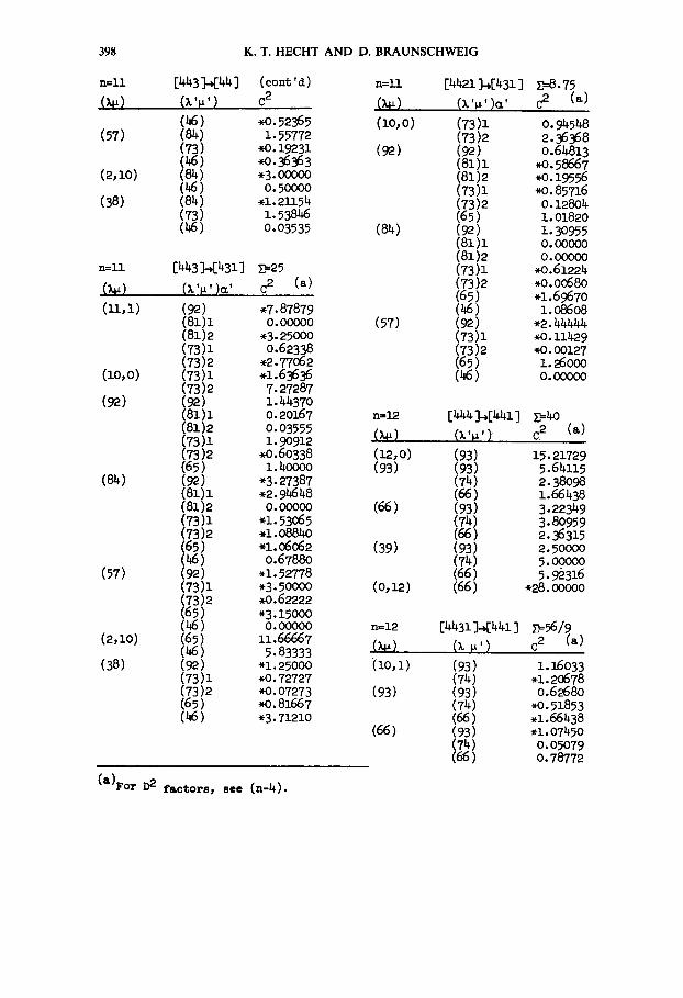
398 K.T. HECHT AND D. BRAUNSCHWEIG
n=n [443 ]~[44 ] (~) (x'~,')
(~6) (57) (84)
(73) (46)
(2,1o) (84) 06)
(38) (84) (73) (46)
m=ll [443~[431] (x~) (~ ' . ' ): ' (11,z) (98)
(81)1 (81)2 (73)1 (73)2
(i0,0) (73)1 (73)2
(98) (98) (81)1 (81)2 (73)1 (73)2 (65)
(8~) (98) (81)1 (81)2 (73)i (73)2 (65) (46)
(57) (92) (73)1 (73)2 (65) (46)
(2,1o) (65) (~6)
(38) (98) (73)1 (73)2 (65) (46)
(cont'd) n=ll 02 (~)
*0.52365 (lO, O) 1.55772
*0.19231 (92) *0.36363 .3.00000 0.50000
-1.21154 1.53846 0.03535 (84)
E=25 c 2 (~)
*7. 87879 o.ooooo (57)
"3. 25000 0.62338
*2.77062 .1.63636 7.27287 1.44370 O. 20167 n=12 O. 03555 i . 90912 ( )q~ )
*0.60338 (12, O) 1.40000 (93)
*3- 27387 *2.946 48 o.ooooo (66)
* l . 53065 *Z. 08840 *1.06062 (39) 0.67880
.i. 52778 *3- 500oo (0,12) .O.62222 *3.15000 O. 00000 n=12 11.66667 (),~) 5.83333
*i. 25000 (10, i) *0. 72727 *0.07273 (93) *0.81667 ,3- 71210
(66)
[4421]-~[431] E--8.75 ( x ' . ' ) ~ ' c 2 (a) (73)1 0.94548 (73)2 2.36368 (98) O.64813 (81)1 *0.58667 (81)2 *0.19556 (73)1 *0.85716 (73)2 0.128o4 (65) 1.o182o (9R) 1.30955 (81)1 o.ooooo (81)2 o.ooooo (73)1 *0.61224 (73)2 .0.00680 (65) -1.69670 (46) 1.08608 (98) *2.44444 (73)1 *0.11429 (73)2 *0.00127 (65) 1.26ooo (46) o.ooooo
(~,~,) c 2 (~)
(93) 15.21729 (93) 5.64115 (74) 2.38o98 (66) 1.66438 (93) 3.22349 (74) 3.80959 (66) 2.36315 (93) 2.5oooo (74) 5.00oo0 (66) 5. 92316 (66) *28. ooo00
[4431~[441] 2=%19 (~ .,) c 2 (a)
(93) 1.16033 (74) .1.2o678 (93) o.6~8o (74) *0.51853 (66) .1.66438 (93) -1.07450 (74) 0.05079 (66) 0.78772
(a)For D2 f&ctors, see (n-4) .
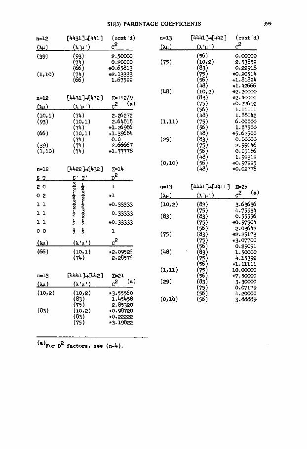
SU(3) PARENTAGE COEFFICIENTS
n=12 [4431]-~4413 (eont'a) n=13 (x~) (x'~') c 2 (x~)
(39) (93) 2.50000 (74) 0.20000 (75) (66) *0.65813
(1,10) (74) *2.13333 (66) 1.67522
(48) n=12 [b/~31]-~[432] ~--112/9 (x~) (x'~') c 2 (a)
(10,1) (74) 2.26272 (93) ( i 0 , i ) 2.64818 (1,11)
(74) .1.26986 (66) (zo,1) .z.39684
(74) o.o (29) (39) (74) 2.66667 (1,1o) (74) .1.77778
(o,1o) n=12
ST
[4422 I~[432 ] ~---]_4 S' T' D 2
o ~ ½ 1 2 n=13 o 2 ½ Z . I (~) 2 1 1 ~ ½ *0.33333 (10,2)
2 1 1 ½ ~ 0.33333 2 (83) 1 1 ½ ½ *0-33333
o o ½ ½ i (75) (~) (x'~') c 2
(66) (1o,1) .2.o9526 (48) (74) 2.28576
(1,11) n=13 [4441]-~[442] 'Z=-21 (~ ) ( x ' . ' ) 0 2 (a) (29)
(lo,2) (lo,2) *3.55560 (83) 1.45458 (o,lb) (75) 2.85320
(83) (10,2) *0.98720 (83) *0.22222 (75) *3.19822
[4441 ]-~[442 ] (xm')
(56) (1o,2) (83) (75) (56) (48) (1o,2) (83) (75) (56) (48) (75) (56) (48) (83) (75) (56) (48) (56) (48)
(cont'd) C 2
O. 00000 2. 53852 O. 22918
.0.20514
. i . 81824
. i . 42666 *2. 20000 *2.4OO0O *0. 276 92 i. iiiii Z. 88O42 6. ooo0o i . 8750O
*5.6250O O. 00000 2. 991h6 o. o5z86 1.9"2312
*0.97225 *0. 02778
[4441]~[44ZZ] ~-25 (x,~) c2 (a)
(83) 3.63636 (75) 4.75534 (83) 0.55556 (75) *o.979o4 (56) 2.03642 (83) *2.29173 (75) .3.07700 (56) 0.29091 (83) 1.5oooo (75) 4.z5392 (56) .1.zzlzz (75) zo.o0o0o (56) .7.50000 (83) 3.30000 (75) 0.07179 (%) 4.2(xx)o (56) 3.88889
399
(a)For D 2 factors, see (n-4).

400 K.T. HECHT AND D. BRAUNSCHWEIG
n=13
(83)
(75)
(48)
(o,1o)
(29)
n=14
(lO, O) (84)
(65)
(57)
(38)
(2,lO)
[4432 ]-.[442 ] (~ '~)
(lO,2) (83) (75) (%) (lO,2) (83) (75) (56) (48) (lO,2) (83) (75) (%) (48) (O, lO) (%) (48) (83) (75) (%) (48)
,~-8.4 n=14 [4442~4421] ,~=-40 02 (a) (~) ( ~ . ) 02 (a) 0.98720 (i0,0) (8h) 3.77111
*0.88889 (84) (I0,0) I.OO884 .0.26108 (92) 2.18259 0.73311 (84) 1.56700 0.63463 (57) 5.07226
*0.22917 (65) (i0,0) .1.62964 *0.82054 (92) -1.69755 o.49165 (84) *0.04274 1.42663 (57) 2.01704 2.20000 (38) 2.09560 0.15000 (57) (92) 2.03704
-1.10772 (84) 3.46160 *0.01111 (57) 2.73514 o.47on (38) o.6o6o8 0.29630 (38) (84) 0.67308 2.02222 (57) .1.09688
-1.44444 (38) *2.96296 1.35000 (2,10) (84) i0.00000
-1.05300 (57) 3.07699 *0.71297 (38) 3.33333 1.05772
[4442].4[443] D=I4 (k,~,) c ~ (a) (84) 3.01687 (ii, i) .2.00000 (lO,O) .o.00388 (92) 0.79367 (84) 1.2536o (57) .1.o1444 (ii, i) 0.76923 (lO, O) .o.1567o (92) 0.021469 (84) 0.85471 (57) .1.49189 (38) o.ooooo (ii, i) .2.00000 (92) -1.15740 (84) 0.17308 (57) o.1~76 (38) .1.48489 (2,10) -1.30772 (84) .2.15385 (57) 0.21939 (38) o.14815 (2,10) 0.95729 (84) .2.0oooo (57) 2.b6160 (38) 0.66667 (2,10) *2.37037
n=14 [44411]~[4421] E=32 (kF) (k'~') C 2 (a)
(92) (92) 1.94425 (84) 5.38466
(73) (92) *2.25689 (84) 0.19883 (57) 0.81457
(65) (lO, O) 0.69842 (92) o.ooooo (84) *3.58981 (57) ~ 1.oo2%
(a) For D 2 factors, see (n-4).
denotesnegative value for C or D,
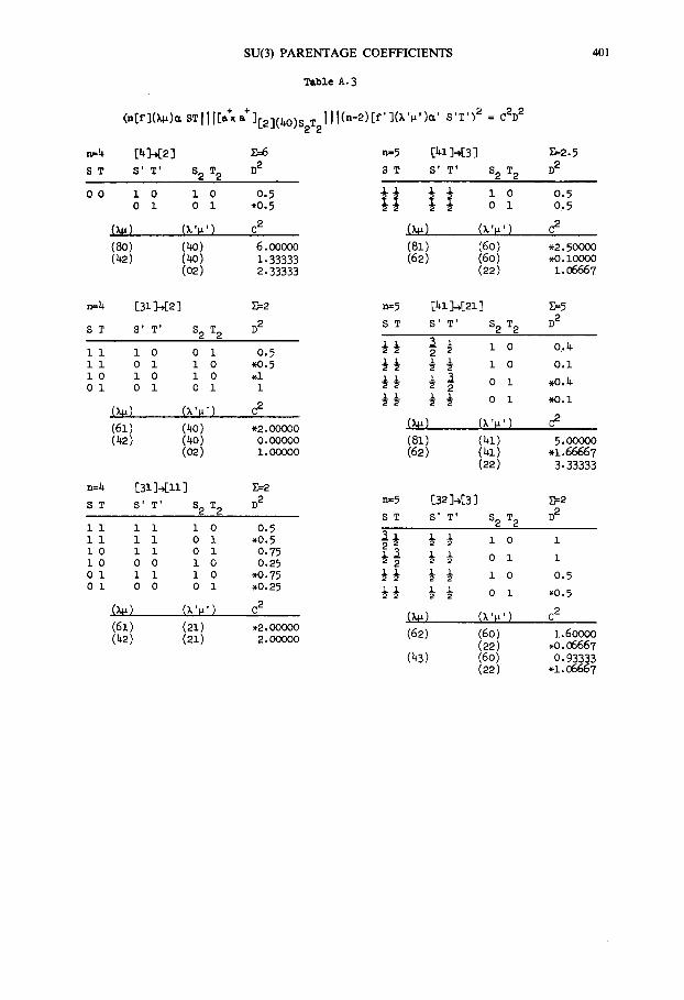
SU(3) PARENTAGE COEFFICIENTS 401
r~4
ST
O0
n=4
ST
ii ii i0 01
n=4
ST
11 11 i0 i0 Ol 0 1
Table A. 3
<.[f](~)~ sTII l [J. "+][2](40)S2T211 I(n-2)[f' ](X'. ' )~' S'T'> ~ = C2D 2
[~]-.[2] ~ n=5 [~i]-.[3]
S' T' S 2 T 2 D 2 S T S' T' S 2 T 2
0 1 o i *0.5 ~ ~ o i
(X~) (k'~,') c 2 (X~) (~.'~,')
(80) (40) 6.00000 (81) (60) (42) (40) 1.33333 (62) (60)
(02) 2. 33333 (22)
5=2.5
D 2
0.5 o,5
c 2
*2. 50000 *0. i0000 z.o6667
[3]- ]~2 ] z=2 n=5 [~z ]-.[21]
S' T' $2 T2 D 2 S T S' T' S 2 T 2
1o o]- o.5 ½½ ~ ]-o o i i o .o.5 ½½ ½ ½ ]- o ]-o lo .i ½½ ½~ o]- 0 1 0 1 1
(6z) (40) .2.ooooo (~) (x '~ ' ) (42) (40) o.ooooo (8]-) (4].)
(oz) z.ooooo (62) (41) (22)
[3z ] - . [n ] z:2 S' T' $2 T2 D 2 n:5 [32]-+[3]
S T S' T' S 2 T 2 1 1 1 0 0.5 i i o i *0.5 ~½ ½½ i o i i o i 0.75 ~3 o i o o 1 o 0.25 2~
z z i o .o.75 ½½ ½ ½ i o o o o i *0.25 !~ ½ ½ o l
(~) (x'~') c 2 (~) (x'.')
(61) (21) *2.00000 (62) (60) (42) (2z) 2 00000 (22)
(43) (60) (22)
E=5 D 2
O. 4
0.i
*0.4
*0.i
5.0OOOO -1.66667 3.33333
~--2
D 2
1
1
0.5
*o. 5
c 2
1.6oooo ,o. 06667 o. 93333
*i. 06667
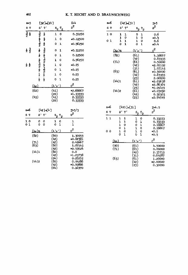
402 K.T. HECHT A N D D. BRAUNSCHWEIG
n:5 [32]-.[m] z=4 S T S' T' S 2 T 2 D 2
~½ ~ ½ z o 0.31250 ½ ½ z o .o.z25oo
½ o z *0.%25o 2
½ o 1 .0.3, 5o ½ ½ o z 0.125oo ½ ~ z o 0.56250
½½ ½ o i o *0.25 ½ o z *0.25
½ ½ 1 o 0.25 ½ ½ o 1 0.25
(~) (x'.') c 2
(62) (41) *2.66667 (22) *i. 33333
(43) (41) 2.33333 (22) O. 33333
n.6 [42 ]-~4 ] z=5/3 S T S' T' S 2 T 2 D 2
i0 Ol
0 0 1 0 1 O 0 0 1 1
(~)~ (X'F') C 2
(82) (80) i. 30953 (42) *0.02381
(71) (42) o.4~67 (63) (80) 1.07143
(42) *0.59524 (44)1 (8o) o.o
(42) .1.23738 (o4) o.25252
(44)2 (8o) o. 94286 (42) *0.00866 (o4) o. 16970
ST
lO
Ol
.=6 ST
ll
O0
[42 ]-~31 ]
S' T' S 2 T 2
1 1 0 1 1 0 1 0 1 1 1 O O 1 O 1
(82) (61) (42)
(71) (61) (42) (31)
(63) (61) (42) (23)
(44)1 (61) (42) (23)
(~)2 (61) (42) (23)
[411~[31] S' T' S 2 T 2
1 1 1 0 1 1 O 1 1 0 0 1 0 1 1 0 1 O 1 0 0 1 0 1
(9o) (61) (71) (61)
(42) (31)
(63) (61) (42) (23)
~5 D 2
0.6 *0.4 0.6
*0.4
c 2
4.16667 0.83333 o.50oo0
*2.01192 i. 57143
*0. 50000 0.83333 2.00000
*2.03638 .2.86365 *0.05455 .o. 03030 O. 30303
.2.54545
Z~4.5 D 2
O. 33333 O. 33333 o. 16667 0.16667
*0.5 *0.5
C 2
4.500oo O. 0 0 0 0 0 2. 35713 0.64287 i. 20000
*2. 00000 O. 30OOO
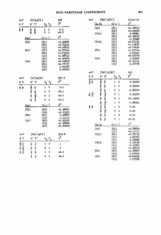
SU(3) PARENTAGE COEFFICIENTS 403
n=7
ST
½½
[43~41] 2-6
S ' T ' S 2 T 2 D R
~ i o 0.5 o I .0.5
(~ ) (x'~,') c 2
(83) (81) -3.~856 (62) .0.83333 (43) *0.23810
(64) (81) .1.o7144 (62) -1.63333 (43) -1.984L? (24) .1.2oooo
(45) (81) -0.42858 (62) *2.77777 (43) 1.o1584 (24) o.ooooo
n=7 [43 ]-*[32 ] 2=% 5 S T S ' T' 82 T 2 D 2
½½
n:7 ST
~ 3 1 o 0.4
½ 3 lO -o.1 ½ ~ o 1 .o.4 ½½ o1 -0.1
(~) (x'~') 02
(83) (62) .4.16667 (43) *3" 33333
(64) (62) 4.16667 (43) Z.lZzn
(45) (62) *0.35556 ( 43 ) .1.38889 (24) .~. 2oooo
[421]-~[41 ] 2-2.4
S ' T' S 2 T 2 D 2
~½ 2 1 3 i 0 i
~ ~ Ol 1
~ ½ ½ 1 o .0.5 ~ Ol .0.5
n=7 [421 ~41 ] ( eont' d) (~): (x'.) c 2
(91) (81) -1.78750 (62) .o. 09o28
(72)z (81) o.48981 (62) *0.38o95 (43) O. 32926
(72)2 (81) .0.61735 (62) -1.14683 (43) .o.1h694
(6~) (81) .i.o71~ (62) O. 83333 (43) *0.05079
(45) (81) 1.2oooo (62) .o. 31111 (43) O. 27778
n:7 [421 ]--,[38 ] 2-3 S T S ' T ' S 2 T 2 D 2
~½ 2
33
~ 3 i o ½3 1o ~3 o 1
Ol
33 oi
3~ io 3 ! i o 2 2
3 0 1 3 2 3½ 1o
33 Ol
(x~)a (x'~')
(91) (62) (51)
(72)1 (62) (51) (43)
(72)2 (62) (51) (43)
(64) (62) (43)
(~5) (62) (43)
o. 31250 O. 12500
o. 56250 O. 31250
*0.12500
o. 56250 0.25 0.25 0.25
*0.25
C 2
*2. 88889 *0. lllll .0.76192 1.60954 o. 38096 o. 12698 o. zoz6o
*i. 28573 .1.06667 o. 44444
*0.62222 1.55556
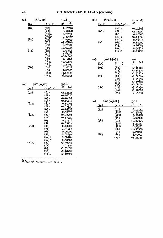
404 K.T. HECHT AND D. BRAUNSCHWEIG
m~8
.,=8
[44 ]<42 ] D,,18 .(x~) (x'~,')=' c 2 (a)
(84) (82) 7.85720 (63) 5.00000 (~)1 2.727~6 (~)2 o. 41~o
(81) (82) o.59o92 (71) *3.07840 (63) i. 20372 ( 52 ) .Z. O7144
(73) (82) 1.94806 (71) 2.81388 (63) *0.66667 (52) 4.17862 (44)1 *1.57830 (~ )2 .0.24050
(46) (82) o.25714 (63) 5.00000 (~)Z *0.6O606 (~)2 6.87O18
[&31]~{42] i"=3.6 (~)~ (x '~ ' ) : ' c 2 (a)
(92) (82) *2.33333 (71) *0.07620 (63) *0.46667 (52) *0.05714
(81)1 (82) 0.59091 (71) *0.62338 (63) *0.43333 (52) 0.38572
(81)2 (82) *0.78788 (Tz) *0.57720 (63) 0.57778 (52) *o.o571~
(73)1 (82) 0.00000 (71) 1.34768 (63) o.o0ooo (52) 0.04592 (~)1 o.56746 (44)2 o.ooooo
(73)2 (82) *0.49242 (71) 0.07730 (63) .1.51668 (52) *0.20408 (44)1 .0.6078o
n:8 [431]<42] (cont'd) (~)= (x'~'):' c 2
(44)2 *o.19698 (65) (82) .2.1429o
(63) o.2ooo0 (44)i *o.03636 (44)2 o.55412
(46) (82) 0.60o0o (63) o.46667 (~)1 0.50911 (44)2 *0.75758
n:9 [441~,[43] Z--6 (~) (~,,,) c 2 (a) (93) (83) .2.86462
(72) *0.16370 (64) -1.91762
(74) (83) *o.52o84 (72) 1.45834 (64) .o. 59662 (45) .o. 08oo0
(66) (83) "3.21430 (64) *o. zoooo (45) 0.95238
n=9 [~41]-~[421] S:15 (~) (~,~,)~, c 2 (a)
(93) (91) 6.11111 (72)1 *0.37415 (72)2 3.99098 (64) o.ooooo
(74) (91) *0.87303 (72)1 3.33333 (72)2 0.55556 (64) -1.9o9o9 (45) 0.28ooo
(66) (64) 8.ooooo (45) *3-33333
(a)For D 2 factors, see (n-4).
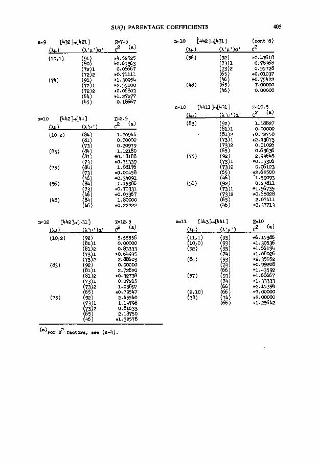
n=9
SU(3) PARENTAGE COEFFICIENTS
[~32]-~[421] .F~-7.5 (~) (x'~')~' c 2 (~) (1o, z) (9]-) .4.52525
(80) ~0.61363 (72)1 0.06667 (72)2 .o.71111
(74) (91) -1.30954 (72)1 *2.55100 (72)2 *0.06803 (64) -1.27277 (45) 0.18667
n=lO [hh2]~[44] L":2.5 (~) (x'~') 02 (~)
(10,2) (84) 1.70944 (81) o.ooooo (73) 0.20979
(83) (Sb.) 1.12180 (81) *0.18188 (73) *0.31339
(75) (8~) z.o8176 (73) .0.oo458 (46) *0.34091
(56) (84) 1.z5386 (73) *0.70331 (;46) *0.03367
(~8) (84) 1.8oooo (46) *0.22222
n=lO ~41g? ].-~431 ] (cont' d) (~) (x'.')~' 02
(56) (92) *0.47618 (73)1 0.78368 (73)2 0.55728 (65 ) *0.01037 (46) *0.75422
(48) (65) 7.ooooo (46) o.ooooo
n=lO [4411]-~[431] 5"=-10.5 (~ ) ( x ' . ' ) = ' c ~ (~) (83) (92) 1.18827
(81)1 0.00000 (81)2 .0.72750 (73)1 *2.43873 (73)2 0.01086 (65) 0.63636
(75) (92) 2.94645 (73)1 *0.15306 (73)2 0.06123 (65) *2.62500 (46) '1.59o93
(56) (92) 0.23811 (73)1 "1.56735 (73)2 *0.68028 (65) 2.07411 (46) .0.37713
n:zo [441~[~31] z:12.5 (~) (x'.')=' c 2 (~)
(lO,2) (92) 5.55556 (81)1 o.ooooo (81)2 o.83333 (73)1 *0.64935 (73)2 2.88603
(83) (92) o.ooooo (81)1 2.72820 (81)2 .0.32?38 (73)1 0.07215 (73)2 1.o3897 (65) *0.79547
(75) (92) 2.45540 (73)1 1.14798 (73)2 0.81633 (65) 2.18750 (46) -1.32578
n : l l [4~3]-~[441] 2=-10 (~ ) (x '~ ') c 2 (~)
11,1) (93) -,,6.15386 i0,0) (93) -1.30536
(92) (93) .z.6619~ (74) .1.o8o26
(84) (93) *2.35052 (74) *0.99208 (66) "1.43592
(57) (93) .1.66667 (74) "1.33333 (66) *2.15394
(2,1o) (66) .7.o0ooo (38) (74) .2.ooooo
(66) .1.25642
(&)For D 2 factorss see (n-~).
405
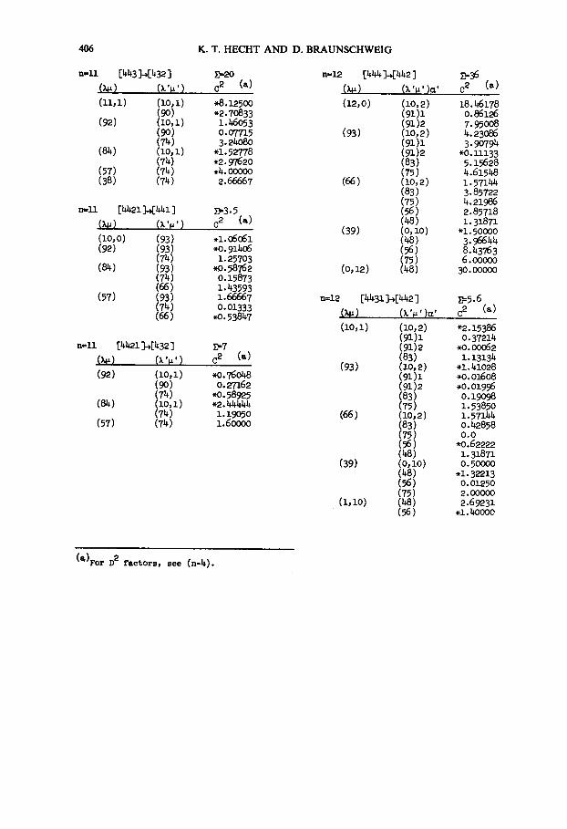
406 K.T. HECHT AND D. BRAUNSCHWEIG
n=l l [443]-~432] Z=-20
(~) (x'~') c 2 (a) (11,1) (zo,1) *8.125oo
(90) *2.70833 (92) (1o, z) 1.46o53
( 90 ) o. 07715 (74) 3.2~08o
(84) (lO, 1) .1.52778 (74) .2.97620
(57) (74) .4.0000o (38) (74) 2.66667
n=ll [4421 ],.~441 ] Z=3.5 (~) (~,'~') 02 (-)
(I0,0) (93) .1.06061 (92) (93) *0.91~06
(74) 1.25703 (8~) (93) .0.58762
(74) o. 15873 (66) i. 43593
(57) (93) 1.66667 (74) 0.01333 (66) .0.53847
~=11 [4~1]-,[432] ~=7
(~) (x'~') c 2 (a) (92) (1o, z) *0.76048
(90) o.rn.62 (74) .0.58925
(8~) (lO,1) .2.44~4 (74) 1.19o5o
(57) (74) 1.6oooo
n:12 [444]~442] S=36 (~) (~,~,):, c 2 (a) (12,o) (zo,2) 18.h6178
(91)1 0.86126 (91)2 7.95008
(93) (10,2) 4.23o86 (91)1 3.90794 (91)2 *0.11133 (83) 5.15628 (75) 4.615~8
(66) (1o,2) 1.571h~ (83) 3.85722 (75) 4.21986 (56) 2.85718 (48) 1.31871
(39) (0,i0) -1.50000 (48) 3.96644 (56) 8.h3763 (75) 6.ooooo
(o,~) (48) 30.00000
,~z2 [443z~[4~] z--5.6 ( ~ ) (x '~ ' )~ ' c 2 (~)
(lO, l) (10,2) "2.15386 (91)1 0.37214 (91)2 .0.0o062 (83) 1.13134
(93) (10,2) -1.410"28 (91)1 .0.01608 (91)2 .0.01996 (83) 0.19o98 (75) 1.53850
(66) (lO,2) 1.5~44 (83) o.42858 (75) o.o (56) ~.622z2 (48) 1.31871
(39) (o,10) 0.50000 (48) -1.32213 (56) 0.01250 (75) 2.000o0
(i, I0) (48) 2.69231 (56) .1.~oooo
(&)For D 2 fac to rs , see (n-4) .
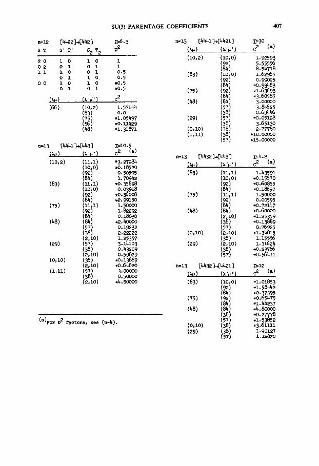
SU(3) PARENTAGE COEFFICIEbrTS 407
-=12 [4~2 ]-,[442 ] ~6.3 S T S' T' S 2 T 2 D 2
20 1 0 1 0 1 02 0 i 0 i i ii i 0 0 i 0.5
o i i o 0.5 00 i o i o *0.5
O 1 O I *0.5
(x~) (~'F') c2
(66) (1o, 2) 1.57144 (83) o.o ( 75 ) -1.05497 (56) .0.11429 (48) -i. 31871
.=13 [4441 ]-~43 ] 2=10.5 (x~) (x#, ' ) c 2 (a) (10,2) (11,1) *3.27284
(zo, o) .0.1852o (92) 0.50505 (84) 1.70942
(83) (n.,z) *0.35898 (10, O) O. 03918 (92) .o.~oo8 (8~) .2.9915o
(75) ( iz,1) z.5oooo (92) 1.82292 (84) O. 18030
(48) (84) .2.~x~oo (57) o. 19232 (38) 2.2z_~22 (2,10) 1.25357
(29) (57) 3.14103 (38) 0.43209 (2,1o) 0.59829
(0,I0) (38) *0.13889 (2,1o) .o.6482o
(1,11) (57) 3.ooooo (38) 0.5oooo (2,1o) .4.50000
(a)For D 8 factors, see (n-4).
r~13 [4441 ]-,[4421 ] (x~) (x'~,')
(1o,2) (1o, o) (92) (84)
(83) (zo,o) (92) (8~)
(75) (~) (84)
(48) (8~) (57) (38)
(29) (57) (38)
(O,10) (38) (i,11) (38)
(57)
n=13 [4432]~[443] (x~) (~'~')
(83) (n,z) (zo, o) (92) (84)
(75) (11,1) (92) (84)
(~8) (8~) (2,zo) (38) (57)
(o,1o) (2,1o) (38)
(29) (2,1o) (38) (57)
n=13 [4432]-~4421] (x~) (x'.')
(83) (lo, o) (92) (84)
(75) (92) (84)
(~) (s~) (38) (57)
(0,10) (38) (29) (38)
(57)
2=3O c 2 (a)
i . 92593 5.55556 8.54718 1.6e965 o. 99o25
*O. 93483 .1.63693 *3.60585 3 • 00000 3.8h625 o.69hh6
*0.05128 3.6513o 2.77780
*I0. CO000 "15 • 00000
~=-4.2 c 2 (a)
i. 43591 *0.15670 *o.6o855 *0.18697
1.5oooo 0.00595
*o. 72117 *0.60000 *1.25359 *0.13889 o.76925
*1. 34815 1.15556 1.31624
*0. u3766 .0.56~n
2=-12 c 2 (a)
*i. 01853 *i. 58~2 *0. 37395 *0.65475 -1.44237 *4.80000 *0.27??8 .1.53852 *3.61111 i. 9O127 Z. ~2820
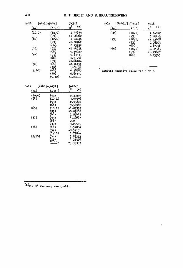
408 K.T. HECHT AND D. BRAUNSCHWEIG
n=14 [4442]-,[444] ~,3.5 (~) (x '~') 0 2 (a)
(i0,0) (12,0) 1.37879 (93) .1.06062
(84) (12,o) 1.4~44 (93) .0.58762 (66) 0.23932
(65) (93) *i.~/~233 (66) 0.59829
(57) (93) 0.83333 (66) 0.71796 (39) *0.64104
(38) (66) *0.94233 (39) 1.02832
(2,10) (66) 0.38889 (39) 0.85472 (0,12) .1.21212
n=14 [4442]-~4431] 2=22.5 (x~) (x '~ ' ) c 2 (a)
(i0,0) (93) 5.30303 (84) (lO, l ) 3.05596
(93) 2.93807 (66) 3.58982
(65) ( i0, i ) -1.83333 (93) ~K).03205 (66) 1.95443
(57) (93) 4.16667 (66) o.o (39) 3.20521
(38) (66) 1.57054 (39) *0.57131 (1,10) 1.72844
(2,10) (66) 5.83333 (39) 4.27358 (i,10) *3.33333
n:14 [44411]~[b431] ~--18 (~) (~,~,) c 2 (a)
(92) (lO, l ) 1.1~072 (93) 5.h8442
(73) ( i0, i ) -1.32408 (93) O.08103 (66) 1.67046
(65) (i0, I) 0.52383 (93) *1.79h87 (66) 2.23365
* denotes negative value for C or D.
(a)For D 2 factors, see (n-4).
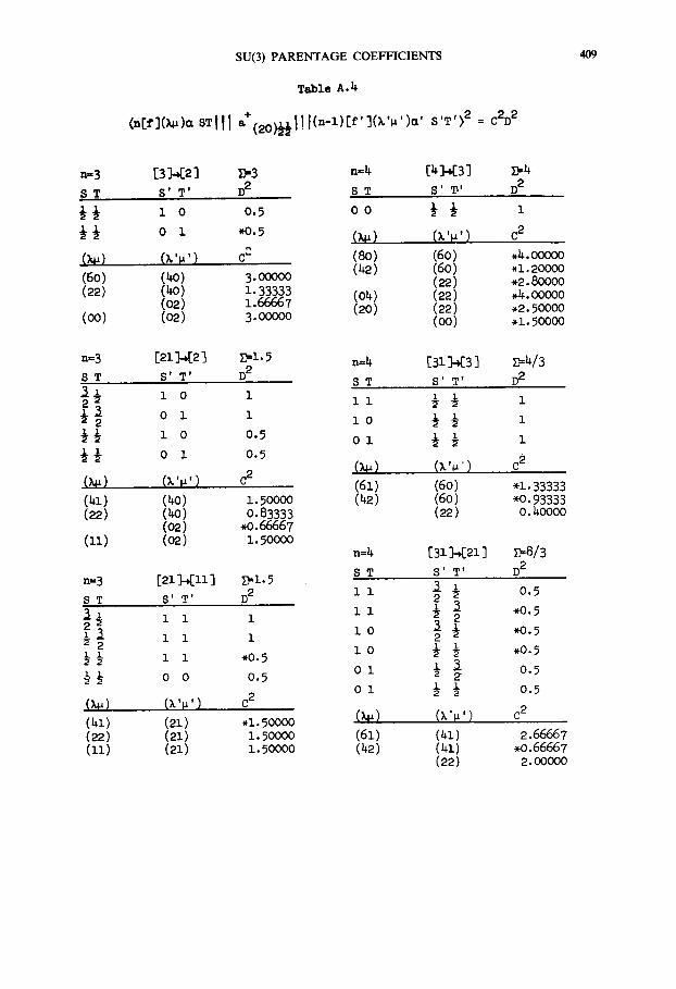
SU(3) PARENTAGE COEFFICIENTS
T~ble A.~
(,,[~](,.~),~ st i l l ~+ ( 2 o ~ I ! l(n-1.)If' ] 0 . ' . ' ) - ' s 'T'>2 : c2D2
409
n=3 [3]-~2] D,3 n:4 [4]~[3]
S T S' T' D 2 8 T 8' ~'
½3 1. o 0.5 o o 3 3
3 ½ o ~ .0 .5 (~) (x'~')
(~) (x'~') c ~ (8o) (60) (~+2) (60)
(60) (4o) 3.0ooo0 (22) (22) (40) 1.. 33333 (04) (22)
(02) 1.66667 (20) (22) (00) (02) 3.00000 (00)
n=3
8 T
33
33
(~1.) (22)
(1.1)
[zz ]-.[z ] s=z. 5 n:4 [31 ].413 ] S' T ' D 2
ST S' T'
1o i 11 ½½
oi l 1o ½½
z o 0.5 o z ½ 3 0 1 0.5
(x'~,') 02 (~) (~'~") (6z) (60) (40) ]..5o0oo (42) (60) (4o) o, 83333 (22) (02) *0.66667 (02) z. 500oo
n=b, [3]- ~[21. ] S T S' T'
n=3 [21. ] - , [ i i ] Z'=I. 5 3 z S T 8' T' D 2 i i 2
~ 3 1. 1. i 11. 3 3~_2 ~ 3 1. z 3. 1.o " ~ - 2 ~ 2 1.o 3 3 1 1
~ i i *0.5 1 I i Ol ~ Z ~ 0 0 0.5
Ol z i. (~) (x'~,') c 2 2
(b,1.) (2z) .z . 50000 (x~) (x'~,') (22) (21.) 1.. 5ooo0 (61.) (4].) (1.1.) (21) 1..5oooo (~.2) (~.z)
(22)
D 2
I
C 2
.4.00000 *i. 20000 *2 • 80000 .4.00000 -2. 50000 *i. 50000
S:4/3 D 2
1
1
1
c 2
-1.33333 *0.93333
0.4oooo
~8/3 D 2
0,5
*0,5
*0,5
. 0 .5
0.5
0.5
C 2
2.66667 *0.66667
2. 00000
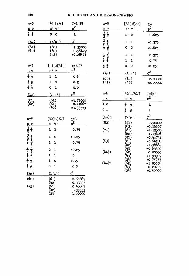
410 K.T. HECHT AND D. BRAUNSCHWEIG
a=5 S T
½½ (x~)
(sz) (68)
n:5
S T
3½
½3 ½½
(81) (68)
n:5
ST
[41 ]..~[4 ] 2=1.85 n=5 [32 ]-,[22 ]
S' T' D 8 S T S' T'
oo z ~ '3 80
(x'~,') c 8 ~ ½ i z 8
(8O) Z.85000 ½ .t. 0 2 (8o) o. 96489 8 (~e) .0.8857z 3 3 ]. z 2
z l ~ i Z
[4~ ]~[31 ] ~3.75 3 ½ o o S' T' D 2 (X~) (X'~,') z z 0.6 (68) (~,8) z o 0.8 (43) (48) 0 i 0.8
(X'~,') O 8
(61) *3.75000 (61) o.4z667 (42) *3- 33333
[32]-b[31 ] 2=3 S' T' D R
3 3 ]. z 0.75 2 3-3 ]. o *o.z5 2 ½~ z i 0.75 2 ½~l o i *0.85 8 ½3 zz o
3 3 i o .0 .5 3½ o z 0.5
(~) ix'~,') c 8 (68) (61) 2.66667
(42) O. 33333 (43) (61) O. #46667
(48) 1.33333 (83) ]..8oooo
~2 D 2
0.625
*0.375
*0.625
O. 375
0.75
*O.25
C 2
2.00000 *2. o0000
n=~ [42 ]-~[41 ] ~--8/3
ST S' T D 2
lo ½½ z
oz ½3 i
( ~ ) ~ (x'~,') c 2
(82) (81) 2.5ooo0 (62) -',~. 16667
(71) (81) .1.125oo (62) 1.13426 (5z) .~.4o74z
(63) (81) .0.64286 (62) , l . 38889 (43) *o.63492
(44) i (62) o.ooooo (43) -1.90909 (24) *0.75757
(~)2 (62) .J..95556 (43) o.2oeo2 (24) .o. 50909
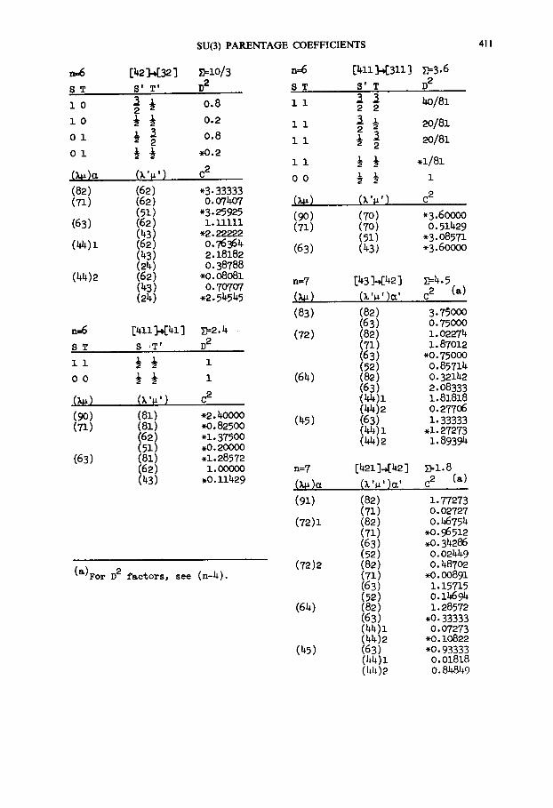
SU(3) PARENTAGE
.=6 [42 ].432 ] mlO/3 S T S' T' D 2
1o ~ ½ 0.8 2
l O ½ ½ 0.2 Ol ½ ~ 0.8
2 o 1 ½ ½ .0 .2
(~)~ (x'F') c 2
(82) (62 ) *3. 33333 (71) (62) O. 07407
(51) *3- 25925 (6 3) (62) i . I i i i i
( 43 ) *2 .22222 (44)1 (62) 0.76364
(43) 2.18182 (24) O. 38788
(b,h.) 2 (62) *0.08081 (43) O. 70707 (24) *2.54545
n=6 [411 ~ [41 ] ~-2. ~ I
S T S ,T' D 2
11 ½½ 1 oo ½½ 1
(~) (x'~') c 2
(9o) (81) .2.40000 (71) (81) .o.825oo
(62) *i. 37500 (51) .o. 2oooo
(63) (81) .i. 28572 (62) 1.0000o (43) .0.11429
(a)For D 2 f ac to r s , see (n-4).
COEFFICIENTS
n=6 [~11 ~311 ] ST S'T
2 2
ii ~ ; 2 } 1 1 ½ 2 2
11 ½½ oo ½½
(90) (70) (71) (70)
(51) (63) (43)
n=7 [43]-.[42]
(83) (82) (63)
(72) (82) (71) (63) (52)
(64) (82) (63) ( ~ ) 1 (4~)2
(45) (63) (4~)1 (~)2
n=7 [421]~[42] (~)~ (x'.')~'
(91) (82) (71)
(72)1 (82) (71) (63) (52)
(72)2 (82) (71) (63) (52)
(6~) (82) (63) (44)1 (44)2
(45) (63) (44)1 (44)2
~3.6 D2
~/81
2o/81 2o/81
.1/81 1
c 2
*3.60000 O. 51429
*3. 08571 *3.60000
~4.5 c 2 (a)
3.75000 0.75000 z.o2274 1.87012
*0.75000 0.85714 0.32142 2.08333 1.81818 0.277O6 1.33333
.1.27273 1.89394
~--1.8 c2 Ca)
i. 77273 O. 02727 O. b6754 .o. 96512 .0.34286 o. 02449 O. 48702 *0.00891 1.15715 o.14694 I. 28572
.o. 33333 o. o7273 *o. 1o822 *o. 93333 o. 01818 o. 84849
411
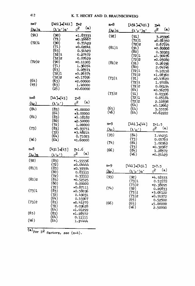
412 K. T. HECHT A N D D. BRAUNSCHWEIG
--7 [421]-~411 ]
(91) (99) (7"1)
(72)1 (9o) (71) (63) (52)1 (52)2
(72)2 (9o) (71) (63) (52)1 (52)2
(64) (63) (45) (63)
(25)
n=8 [44 ]~[43 ] (~) (~'. ') (84) (83)
(64) (81) (83)
(8o) (72)
(73) (83) (72) (64)
(46) (64)
n=8 [431]-*[43 ] (~)= (~'. ') (92) (83)
(72) (81)1 (83)
(8o) (72)
(81)2 (83) (80) (72)
(73)1 (83) (72) (64)
(73)2 (83) (72) (64)
(65) (83) (64)
(46) (64)
~=2 .,.8 [431]-~421] 02 (a) (~)~ (x '~ ' ) : '
-1.83333 (92) (91) ~o.16667 (72)1 0.71429 (72)2
.o.o2o41 (81)1 (91) 0.91429 (80) 0.27472 (72)1 0.07629 (72)2
*0.119o5 (81)2 (91) 1.36o54 (8o) 0.o8571 (72)1
*0.26374 (72)2 *0.17096 (73)1 (91) .2.0oooo (72)1 1.4oooo (72)2
.0.60ooo (64) (73)2 (91)
z:-8 (72)1 c 2 (a) (72)2
(64) *5.00000 (65 ) (6 4) *3.000oo (46) (64) -1.18182 .2.50000 1.00000 n:9 [441~[44] ~=-1.5
*0.93751 (k~) (X'B') C 2 (a) *3.48214 0.71023 (93) (84) 1.44231
*1.60000 (73) 0.05769 (74) (84) 1.oo962
(73) *0.32967 Z=1.6 (66) (84) 1.28572 C 2 (a) (46) *0.21429
"1.55556 ,0.04444 n=9 [4413,[431] ~=7.5 *0.39394 _~_) (k'.')a' C 2 (a) 0.83333 0.33333 (93) (9"2) *4.58333
*0.52525 (73)1 0.53572 0.00000 (73)2 *2.38095
*0.87111 (74) (92) 0.20833 .0.58036 (73)i -3.06122 0"h9031 (73)2 *0.91972 O. 43967 (65) O. 52500
.o. 41270 (66) (65) -5.0oooo 0.03628 (46) 2.500oo
"1.01299 "1.28572 O.11111 1.24444
c2 Ca)
3.25926 .0.06 350 o.6T724
*0.80808 O. 30303
.1.99476 *o.o5o8o 0.26936 2.04546 O. 10158
.z. o8360
.o. 47620 1.97084 o.oo194
.o. 56 278 O. 033O6 O. 05184 2.1o898
.0.12662 3. 55556
*0.62222
(a)F°r D2 factors, see (n-4).
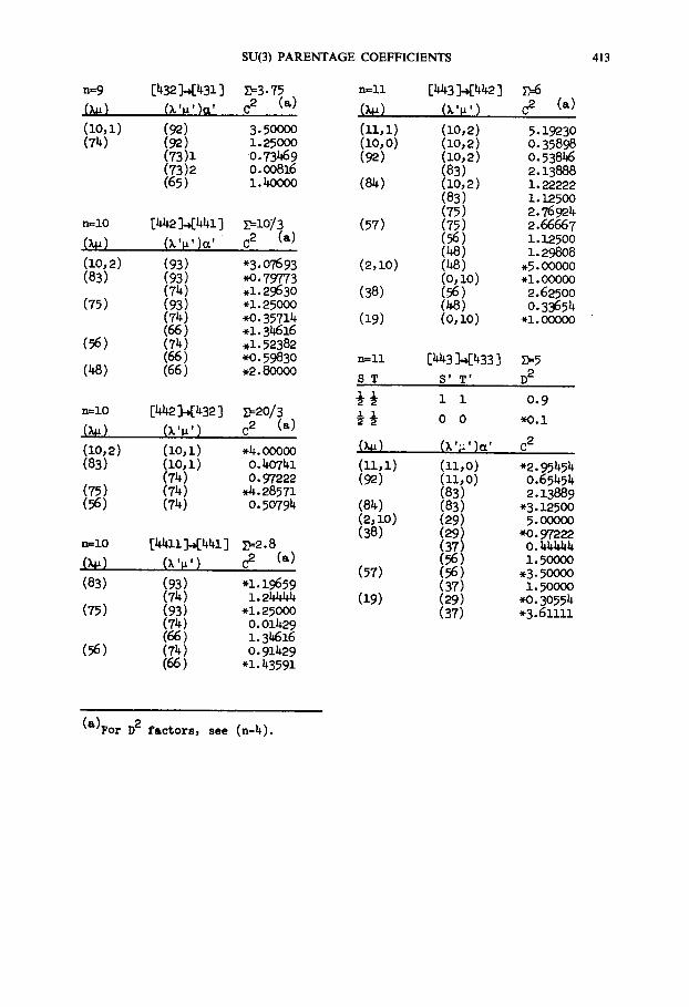
SU(3) PARENTAGE COEFFICIENTS 413
n=9 (~) (lO,1) (74)
[432]-~[431] 2=3.75 (~,~,)~, c 2 (a)
(92) 3.5oooo (92) 1.25ooo (73)1 0.73469 (73)2 0.00816 (65) 1.4oooo
n:zo [~2].,[441] ~1o/3 (~) (~,~,)~, c 2 (a)
(10,2) (93) *3.07693 (83) (93) *0.79773
(74) .1.2963o (75) (93) -1.25ooo
(74) ~<).35714 (66) -1.34616
(56) (74) .1.52382 (66) *0.59830
(48) (66) .2.8oooo
n=lO [4/~2]-~[432] ~--20/3
(~) (~,.,) c 2 (a) (lO,2) (lO,1) .4.ooooo (83) (1o,1) 0.40741
(74) 0.97222 (75) (74) .4.28571 (56) (74) 0.50794
n=zo [4411].,[441] 2=2.8 (~) (x',') c 2 (a) (83) (93) -1.19659
(74) 1.24444 (75) (93) -1.25000
(74) 0.01429 (66) 1.34616
(56) (74) 0.91429 (66) "1.43591
n=ll
(11,1) (1o, o) (92)
(84)
(57)
(2,1o)
(38)
(19)
n=ll
ST
[443]<442] (~,.,) C 2 (a)
(1o, 2) 5.19230 (lO, 2) o. 35898 (lO, 2) o. 53846 (83) 2.13888 (10,2) 1.22222 (83) i . 12500 (75) 2.76924 (75) 2.66667 (56) 1.125oo (48) 1.298o8 (~8) .5.00000 (0, i0) *i. 0OO00 (56) 2.62500 (},,8) 0.33654 ( 0, i0 ) *i • 00000
[443 ]-.[433 ] S' T'
L~-5 D 2
½½ ½½
(~) (11.1) (92)
(84) (2.1o) (38)
(57)
(19)
1 1
0 0
(11.o) (11.o) (83) (83) (29) (29) (37) (56) (56) (37) (29) (37)
0.9 *O.i
c 2
*2.95454 0.65454 2.13889
"3.12500 5.00000
"NO. 97222 o. ~4 1.5oooo
*3- 50000 i. 5ooO0
*0.30554 *3.61111
(a)For D 2 factors, see (n-4).
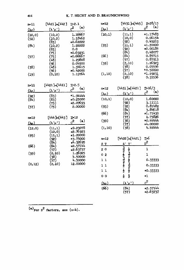
414
n,=ll
(1o,o) (92)
(s~)
(57)
(38)
(19)
n=ll
(92)
(57)
n=12 (~)
(12,o)
(93)
(66)
(39)
(o,12)
K. T. HECHT AND D. BRAUNSCHWEIG
[~21]-,[442] ~2 .1 (xm') c 2 (~)
(lO,2) 1.16667 (lO,2) 1.18462 (83) .0.62222 (10,2) 1.22222 (83) o.o (75) *0.69231 (75) *0.66667 (~8) 1.298o8 (56) 0.04500 (48) z.34615 (56) .0.42ooo (0,10) 1.29764
[4421~[4411] ~-2.5 (~,.,) 02 (a)
(83) *1.941~4 (83) .0.25000 (75) *2.07693 (75) 2.oooo0
(x '~ ' ) 0 2 (a)
(ii, i) .9.23078 (i0,0) .2.76923 (11,1) .1.20000 (92) *3.75000 (84) .4.32695 (84) .2.57144 (57) .2.63737 (2,1o) 1.26925 (38) 4.soooo (57) 4.5oooo (2,10) 12.00000
n=12
(lO,1)
(93)
(66)
(39)
(1,1o)
[4431]-b[443] ~--28/15 ( x ' . ' ) 0 2 (~)
( i i , i ) -1.17483 (1o, o) o.o6154 (92) 0.45253 (Ii, i) .1.20000 (92) *0.00185 (84) 0.48O77 (84) 0.85715 (57) 0.87913 (2,10) 1.26923 (38) 0.05556 (57) *0.50000 (2,10) "1.29231 (38) 0.35556
n=12
(1o,1)
(93)
(66)
(39)
(1,1o)
[4432~[4422] ~16/3 (x'~') c 2 (a)
(1o, o) 1.6oooo (92) 3.z2111 (92) o.81~2 (8~) 3.84618 (84) -1.71430 (57) 1.75826 (38) .0.444~ (57) .4.00000 (38) 4.4bAJ44
n=12 [44223~[4421] S T S' T' D 2
20 ~½ 1 02 ~2 1 1 1 ~ ½ 0.33333 i 1 ~ ~ 0.33333 2 1 1 ½ ½ *0.33333 oo ~ ½ -1
(~) (x'~') o 2
(66) (84) .2.57144 (57) *2.63737
(a)For D 2 fac to r s , see (n-4) .
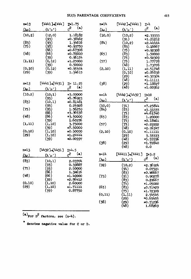
SU(3) PARENTAGE COEFFICIENTS 415
n=13 (~)
(zo,2)
(83) (75)
(48)
(1,11)
(o, 1o) (29)
n=13
(1o,2)
(83)
(75)
(48)
(z,u.)
(o,1o) (29)
,I=13
(83)
(75)
(48)
(o,1o) (29)
[4~1~[444] 2=1.75 (x ' . ' ) 0 2 (a)
(12, o) 1.18182 (93) ~0.38462 (93) 1.34616 (95) ~o. 93750 (66) .0.67308 (66) .o. 70000 (39) O. 96154 (0,12) .1.25000 (39) O. 50000 (o, 12) .o. 95454 (39) i. 3b615
[~d441~4431] ~ 11.25 (x'~,') c 2 (a) (10, i ) *3. o00oo (93) *5.76923 (lO,1) .o.81481 (93) O. 24928 (93) i. 56250 (66) *3.36538 (66) *3.5oooo (39) 1.60256 (1, i0) 3.75OO0 (39) *7.50000 (1,1o) .o.5ooo0 (z, 1o) .1.24444 (39) ,o. oo997
[44~ ]-<4431] Z:4.5 (x ' . ' ) c 2 (a)
(10, i) 2.03704 (93) O. 39887 (93) 2.5oooo (66) i . 34616 (66) .1.4oo0o (39) *2.56 412 (1,1o) 2.60oo0 (i, i0) *i. 71111 (39) O. 87750
n=14
(1o, o)
(84)
(65)
(57)
(2,1o)
(38)
n=14
(1o, o) (84)
(65)
(57)
(2,1o)
(38)
n=14
(92)
(73)
(65)
(o,11)
(38)
[~442]~[4441] L'=4 ( x ' . ' ) c 2 (a)
(10,2) *2.33333 (91) -1.21212 (1o, 2) .2. ~4~4 (83) o.z6667 (75) .o. 923o8 (83) 1.soooo (75) .o. 92309 (75) 1.77778 (48) 1.73078 (l, zz) .2.51748 (0,i0) *0.06838 (29) *0.3O3O4 (48) -1.11111 (29) *1.z8827 (48) .1.00962
[4442 ~[4432] s:zo (x'~') c 2 (a)
(91) ,7.25844 (83) *3. 33333 (75) .4.6154o (83) 1.2oooo (75) *0.181461 (75) .2.22222 (48) *2.16347 (0, i0) *i. 11111 (29) 3.33333 (48) *5.55556 (29) -1.7284o (48) o.o
[44411].,[4441] ~-3.2 (x'~') c 2 (a)
(10,2) -2.369e4 (91) 0.07521 (83) .o. 46667 (91) o. 9o278 (83) 0.21667 (75) -1.o5ooo (83) .o. 51429 (75) .1.72309 (I, i i ) 2.54545 (29) *o.65455 (29) *o.71296 (48) 1.68269
(a )For D 2 f a c t o r s , see (n-4) .
denotes nega t ive value fo r C or D.
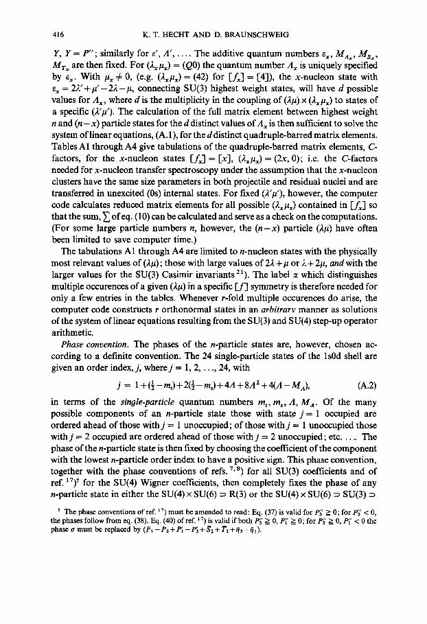
416 g . T . HECHT AND D. BRAUNSCHWEIG
Y, Y = P"; similarly for e', A', . . . . The additive quantum numbers ex, M.~, Msx, Mrx are then fixed. For (2x#~) = (Q0) the quantum number A~ is uniquely specified by e~. With /~ =~ 0, (e.g. (2x#~)= (42) for [_f~] = [4]), the x-nucleon state with ex = 22'+ g ' - 2 2 - # , connecting SU(3) highest weight states, will have d possible values for A~, where d is the multiplicity in the coupling of (2#) x (2~ #~) to states of a specific (2'#'). The calculation of the full matrix element between highest weight n and ( n - x ) particle states for the d distinct values of Ax is then sufficient to solve the system of linear equations, (A. 1), for the d distinct quadruple-barred matrix elements. Tables A1 through A4 give tabulations of the quadruple-barred matrix elements, C- factors, for the x-nucleon states I f x] = [x], (2~#x)= (2x, 0); i.e. the C-factors needed for x-nucleon transfer spectroscopy under the assumption that the x-nucleon clusters have the same size parameters in both projectile and residual nuclei and are transferred in unexcited (0s) internal states. For fixed (2'#'), however, the computer code calculates reduced matrix elements for all possible (2x#~) contained in [fx] so that the sum, ~ ofeq. (10) can be calculated and serve as a check on the computations. (For some large particle numbers n, however, the ( n - x ) particle (2#) have often been limited to save computer time.)
The tabulations A1 through A4 are limited to n-nucleon states with the physically most relevant values of (2#); those with large values of 22 + # or 2 + 2#, and with the larger values for the SU(3) Casimir invariants 21). The label ~ which distinguishes multiple occurences of a given (2#) in a specific [_/] symmetry is therefore needed for only a few entries in the tables. Whenever r-fold multiple occurences do arise, the computer code constructs r orthonormal states in an arbitrarv manner as solutions of the system of linear equations resulting from the SU(3) and SU(4) step-up operator arithmetic.
Phase convention. The phases of the n-particle states are, however, chosen ac- cording to a definite convention. The 24 single-particle states of the ls0d shell are given an order index, j, where j = 1, 2 . . . . . 24, with
j = I+(½-mt)+2(½-m~)+aA+8A2+4(A-Ma) , (A.2)
in terms of the single-particle quantum numbers mr, ms, A, M a. Of the many possible components of an n-particle state those with state j = 1 occupied are ordered ahead of those withj = 1 unoccupied; of those withj --- 1 unoccupied those withj = 2 occupied are ordered ahead of those withj = 2 unoccupied; etc . . . . . The phase of the n-particle state is then fixed by choosing the coefficient of the component with the lowest n-particle order index to have a positive sign. This phase convention, together with the phase conventions of refs. 7, a) for all SU(3) coefficients and of ref. 17)t for the SU(4) Wigner coefficients, then completely fixes the phase of any n-particle state in either the SU(4) x SU(6) ~ R(3) or the SU(4) × SU(6) ~ SU(3)
t The phase conventions of ref. 17) must be amended to read: Eq. (37) is valid for F f > 0; for F3' < 0, the phases follow from eq. (38). Eq. (40) of ref. 17) is valid if both P~" > 0, ~ ' > 0; for P~' > 0, F f < 0 the phase a must be replaced by (P1--P3 +1~1--J~3+ ~2 + ~2 +f]3- f]l).
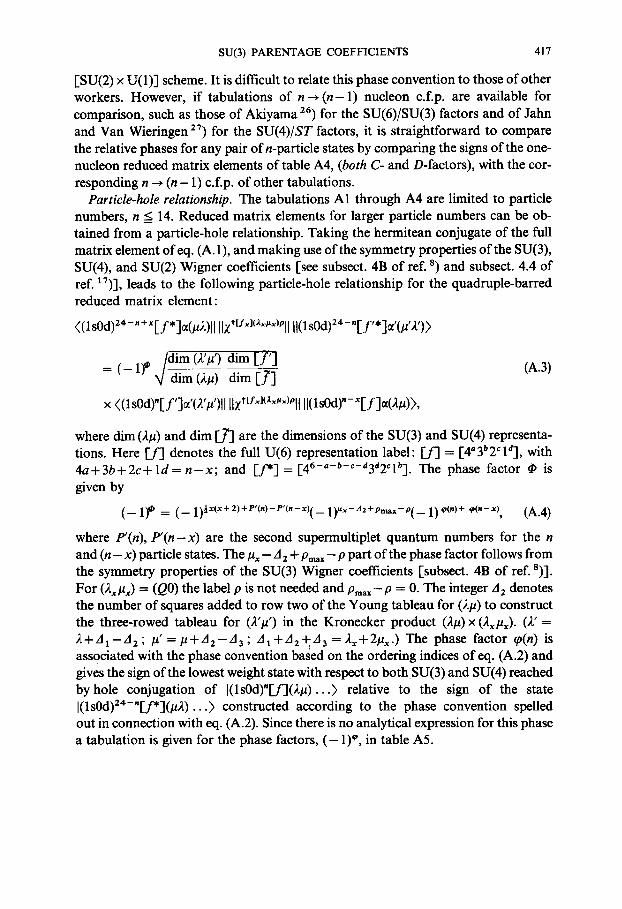
SU(3) P A R E N T A G E COEFFICIENTS 417
[SU(2) x U(1)] scheme. It is difficult to relate this phase convention to those of other workers. However, if tabulations of n--, ( n -1 ) nucleon c.f.p, are available for comparison, such as those of Akiyama 26) for the SU(6)/SU(3) factors and of Jahn and Van Wieringen 27) for the SU(4)/ST factors, it is straightforward to compare the relative phases for any pair of n-particle states by comparing the signs of the one- nucleon reduced matrix elements of table A4, (both C- and D-factors), with the cor- responding n --, ( n - 1) c.f.p, of other tabulations.
Particle-hole relationship. The tabulations A1 through A4 are limited to particle numbers, n < 14. Reduced matrix elements for larger particle numbers can be ob- tained from a particle-hole relationship. Taking the hermitean conjugate of the full matrix element of eq. (A. 1), and making use of the symmetry properties of the SU(3), SU(4), and SU(2) Wigner coefficients [see subsect. 4B of ref. s) and subsect. 4.4 of ref. 17)], leads to the following particle-hole relationship for the quadruple-barred reduced matrix element:
((ls0d)24-, +x[-f*]~t(#2)ll IIx*tlx~(axux)Pll II(ls0d)2"-"[f'*]a'(/2')>
= ( - 1) ~ / d i m (2'#') dim [ f ' ] (A.3) N/dim (2#) dim [y ]
x <(ls0d)"[f']ct'(2'/~')ll IlxttsxJtaxux)Pll II(ls0d)"-xl-f]~(;t#)>,
where dim (2#) and dim D 7] are the dimensions of the SU(3) and SU(4) representa- tions. Here I f ] denotes the full U(6) representation label: Dr] = [4°3~2 c ld], with 4 a + 3 b + 2 c + l d = n - x ; and If*] = [46-°-b-c-d3n2Clb]. The phase factor • is given by
(_ 1)e = (_ 1)~xt~+ 2)+P'(n)-P'(n-x)(__ ly, x-a~+pr~,-p(_ 1) 'Pt")+ ~"-~), (A.4)
where P'(n), P'(n-x) are the second supermultiplet quantum numbers for the n and ( n - x) particle states. The # x - A 2 "~ Pmax - - i 0 part of the phase factor follows from the symmetry properties of the SU(3) Wigner coefficients [subsect. 4B of ref. s)]. For (2~#~) = (Q0) the label p is not needed and Pmax--P = 0. The integer A 2 denotes the number of squares added to row two of the Young tableau for (2#) to construct the three-rowed tableau for (2'#') in the Kronecker product (2/0 x (2x#~). (2"= ) . + A 1 - A 2 ; /2' = / . t W A 2 - A 3 , AI+A2+A 3 = 2x+2/~x. ) The phase factor tp(n) is associated with the phase convention based on the ordering indices of eq. (A.2) and gives the sign of the lowest weight state with respect to bothSU(3) and SU(4) reached by hole conjugation of I(ls0d)"[f](2#)...> relative to the sign of the state I(ls0d)24-"[f*]~2). . .> constructed according to the phase convention spelled out in connection with eq. (A.2). Since there is no analytical expression for this phase a tabulation is given for the phase factors, ( - 1)*, in table A5.

418 K.T. HECHT AND D. BRAUNSCHWEIG
[ q (~,.) (-1) + I f ]
[ 2 ] ( 40 ) [32 ]
(02) +
[11] (21) +
[ 3 ] ( 60 ) +
(22)
(00) [42]
[21] (41)
(22) + ( l l )
[4 ] (8o) +
(42 ) -
(04) + [411]
(2o ) +
[ 31 ] (61 ) -
(42) - [43]
(23) -
( 31 ) -
(+2) - ( 2 0 ) - [421]
[22] (42) +
( 31 ) +
( 0 4 ) -
( 20 ) -
[41] (81) * [44]
( 62 ) -
(43) +
(51) +
(24) - [431 ]
(32) -
(4o~+ -
TABLE A.5
The phase f a c t o r ( - I ) ~(n)
(Xu) ( - I ) e [ f ] (Xl~) ( -1) e [ f ] (Xp) (-1) ~
( 6 2 ) - [ 4 4 1 ] ( 9 3 ) - [ 4 4 3 1 ] ( i o , i ) -
( 4 3 ) - ( 7 4 ) - ( 9 3 )
(51) + (66) - (66) +
(24) - [432] (10, 1) + (39)
(32) - (74) ( i ,10)
(82) - [442] (10,2) [4441 ] (10,2)
(71) - ( 83 ) + (91 )
(63) + (75) + (83)
(52) + (56) + (75)
( 4 4 ) I - ( 48 ) (48 )
(44)2 - (0, !0) + (29) +
(90) + [4411] (83) + (0,10)
(71) - (75) + (1,11)
(63) + (56) + [4432] (91) +
(83) - [443] (11,1) + (83) +
(72) + (10,0) + (75) -
(64) + (92) (48) -
(45 ) - ( 84 ) + ( 29 ) -
(91) + (57) + (0,10) -
(72) ! + (2,10) + [4442] (10,0) +
(72)2 - (3 ,8) + (84) -
( 64 ) + ( 1 , 9 ) + ( 65 ) +
(45) + [4421] (10,0) + (57) +
(84) + (92) + (38) +
(81) + (84) + (2,10) -
(73) + (57) + [44411] (92) +
(46) - ( 3 8 ) - ( 7 3 ) -
( 9 2 ) - (19) - (65) -
(81) i + [444] (12,o) + (38) +
(81)2 - (93) - (19) -
(73)! (66) + (0,11) +
(73)2 + (39) -
( 65 ) - ( o , 1 2 ) +
(46 ) -
~(n) is de f ined in connect lon w i t h eq. (A .4 ) .
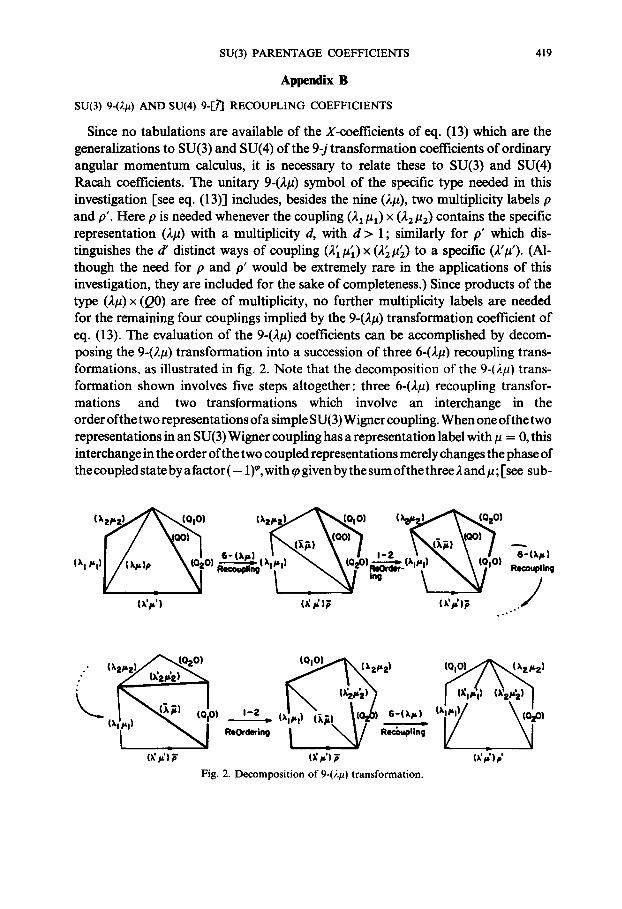
SU(3) PARENTAGE COEFFICIENTS 419
Appendix B
SU(3) 9-(2/z) AND SU(4) 9-[~] RECOUPLING COEFFICIENTS
Since no tabulations are available of the X-coefficients of eq. (13) which are the generalizations to SU(3) and SU(4) of the 9-j transformation coefficients of ordinary angular momentum calculus, it is necessary to relate these to SU(3) and SU(4) Racah coefficients. The unitary 9-(~/~) symbol of the specific type needed in this investigation [see eq. (13)] includes, besides the nine 0.#), two multiplicity labels p and p'. Here p is needed whenever the coupling (~1/zl) x (~.2/~2) contains the specific representation (;t#) with a multiplicity d, with d > 1; similarly for p' which dis- tinguishes the ae distinct ways of coupling (2i # i )x 0.[/~[) to a specific (~'/~'). (Al- though the need for p and p' would be extremely rare in the applications of this investigation, they are included for the sake of completeness.) Since products of the type (~/~)x (Q0) are free of multiplicity, no further multiplicity labels are needed for the remaining four couplings implied by the 9-(~/~) transformation coefficient of eq. (13). The evaluation of the 9-(~#) coefficients can be accomplished by decom- posing the 9-(2/z) transformation into a succession of three 6-(;~#) recoupling trans- formations, as illustrated in fig. 2. Note that the decomposition of the 9-040 trans- formation shown involves five steps altogether: three 6-(2~) recoupling transfor- mations and two transformations which involve an interchange in the order ofthetwo representations of a simple SU(3) Wigner coupling. When one of the two representations in an SU(3) Wigner coupling has a representation label with/z = 0, this interchange in the order of the two coupled representations merely changes the phase of the coupled state by a factor ( - 1) ¢, with tp given by the sum of the three 2 and/~; [see sub-
e'(xl'),,~,j h) ~ \ (o2o )~ (xa , i) ~ \(q~o) ~'-(x~,)
(~'~,') (~ ~)~ (~'~)~ .. . . . "
(~.~')~ Fig. 2. Decomposition of 9-(2/~) transformation.
420 K.T. HECHT AND D, BRAUNSCHWEIG
sect. 4B of ref. 8)]. The decomposit ion of the 9-(4#) transformation illustrated by fig. 2 thus leads to the relation
x . f(4,#,)(42#9 (4#)p su(3)~t(2x0) ((220) ((20)
\(41#~) (4~#~)(z/2')p'/
= ~.. U((4 i/2, X42/22X2'/2'XQO); (2/2)p _ ; (~-fi)_ p)( - 1 )Q' + e2 + Q (B. 1 )
x U((22/22XQ 2 0XXfiXQ i 0); (4~ #~)_ _ ; (Q0)_ _)( - 1 )x[ +,[ + Q I "l" ~ "t"
x U((A, #IXQ, 0X2'#'X2~ #~); (2~ #'1)- p'; (Xfi)_ fi).
[Mult ipl ic i ty labels p in the U-coefficient, U((41 #1)(42/~)(2/2)(2 a #a); (212/212)PI2P12.3; (42a#23)Pz3Pi, 2a) are indicated only where they are needed.]
With (42#2) = (00), and consequently (4,#1) = (4#), (4[/2[) = (Q20); (Xfi) can take on only the value: (Sfi) = (Q0). In this special case eq. (B. 1) reduces to
((4#) (oo) (4#) = (( #XQ, X /2)(Q20);(2,#,);(Q0)). (B.2) Xsu(3)~(Ql0) (Q2 0) (Q0) / U 4 0 2 . . . .
\(4k #~) (Q2O) (4'#')/
A slightly different relation is obtained from a similar decomposit ion of the 9-(4#) transformation, starting with the last coupled state shown in fig. 2,
/,'(4,#,) (4~#~)(M)p X sut3)l(QlO) (Q2 O) (QO) ,1__
\(41.#D (41#D (4'#')p /
! v ! / 0 " v v / U((41 #1X42/22X 4 # X(22 ), (Xp)p_ ; (42 #2)- P X-- 1) x` + "' + Q ̀+ xi +,i
x U((Q, 0)(4, #1)(Xp)(42 #2); (4~ #[)_ fi; (4/2)p_)(- 1) x+"+0' +g+~ (B.3)
x U((2#)(Q, 0)(4'#'XQ2 0); (Xfi)__ ; (Q0)_ _).
Now, with (2~#~)=(00), and consequently (21#1)=(0Q,) , (2[ #[) = (2'#') ; (Xfi) can take on only the value: (~/~) = (22 #2). In this special case eq. (B.3) reduces to
((o(2,) (4~#~)(4#) Xsu(3)~((2,0 ) ((22 0) ((20) ]
\ (oo) (4'#') (4 '# ' ) /
F dim (2#) J~ = U((M)((2,0)(4'#')((220); (42/22); ((20)) [_dim (42~-2) d-i--m ((2,0) ' (B.4)
SU(3) PARENTAGE COEFFICIENTS 421
where the SU(3) U-coefficient with (00) in the 12-position has been expressed in terms of the simple dimension and phase factors given by eq. (A.6) of ref. 1,).
The SU(4) X-coefficient of eq. (13) is somewhat simpler since it contains the scalar representation [0]. (Although multiplicity labels could again be needed in principle, in actual practice they must be expected to be so rare that they have been quietly omitted.) The exact analog of eq. (B.1) gives
[[7'11 [L] [~1 '~ Xsu(,)|[-1 x'] [l=q [1"2 = [0
\[Y;] [?~] [?l = ( - 1)*([l~'][lx'][°))U(['j~2][-l~'l[J~21[l=~]; [~'] ; [0]) (B.5)
x ( - 1),(~,,'x',t~,~)v(E,~,]E1,,]Ey][~]; [?(]; E,~,]),
where ~0([__71][T2][73]) is the phase factor associated with the interchange in the order of the SU(4) Wigner coupling of the representations [~1] and [A~2].
With [A~2] = [0], and consequently [~1] = [J] , [ATe] = [1~2], this collapses to
Xsu( , ) [ [ l " ] [ I "2] [0] ] = U(Ej~][I~'][.~][I'2]; El;]; [0]), (B.6) \ [ .Y;] [1 "2] [ i ' ] /
With [y~;] = [0], and consequently [7'1] = [1"2], D'~] = [_7]; and using the phase conventions of ref. 17), the SU(4) X-coefficient becomes
{[v,] ILl [/]'~ i Xsu(,,[[1 x,] Dxq . (B.7)
\[o] [.T] I~]]) =dimsU('>[r']
Appendix C
SPURIOUS EXCITATIONS OF THE CENTER-OF-MASS MOTION
In the SU(3) strong coupling scheme most states with large values of 2 and # are completely free of spurious c.m. excitations. In those few cases where the (2#) of interest can contain spurious c.m. excitations the SU(3) strong coupling scheme also furnishes the simplest basis for the construction and hence the elimination of such spurious components. The method has been given in detail in ref. 14). Spurious states are generated by acting on the non-spurious states of lower oscillator energy with the excitation operator which raises the oscillator energy of the c.m. excitation but does not act on any of the intrinsic degrees of freedom. The c.m. excitation operator has SU(3) irreducible tensor character (2#) = (10). When acting on a non-spurious state
422 K .T . HECHT AND D. BRAUNSCHWEIG
(2/z) it can create only excitations of SU(3) symmetry (2+ 1, #), ( 2 - 1 , / ~ + 1), and (2 , /~-1) ; i.e. it can raise the (22+/~) values by at most two units. States of lhco of core excitation are then completely non-spurious if
22+/~ > (22+/~)mx+2. (C.1)
The maximum possible values of (22 +/z) for states of no core excitation follow from the e-structure of the single-particle spectrum (see fig. 1), from which it is apparent that
(22+1z)~ x = 4(A-16), for 16 < A < 20,
(22+/~)=a x = 16+(A-20) , for 20 < A < 28.
States of 2hco of core excitation can be doubly spurious (provided (22+/~)~- (22 + p)=,= + 4), but they may also be singly spurious with a c.m. excitation of 1 ho9 based on a core excited state of purely intrinsic excitation of 1 hto. For nuclei with 16 < A < 28 and maximum possible (22+/~) the intrinsic excitations of lhco can increase the above 12~, + P)m,~ values by at most five units (either by lifting a particle out of the 8 = - 1 level of the 0p shell into the 8 = 4 level of the 1 sOd shell, or by lifting a particle out of the ~ = 1 level of the 1 sOd shell into the e = 6 level of the lp0f shell, see fig. 1). Since the c.m. excitation operator can further raise 22+/~ by at most two units, states of core excitations of 2ho9 are completely non-spurious if
(22 + #) > (22 +/~)m~ + 7, for 16 < A < 28. (C.2)
Note that most of the core excited states included in tables 3, 4, 6 satisfy (C.1) while most of those in tables 5, 7 satisfy (C.2).
In cases where spurious states must be considered these have been constructed by the methods of ref. 14). The core excited states of 2°Ne will be considered in some
5 detail. States of [4 ] space symmetry and 0ha~ core excitation are limited to (2#) = (80), (42), (04), (20). The c.m. excitation operator acting on these intrinsic states creates the singly spurious states of 1 hco excitation, I-45] space symmetry, and SU(3) quantum numbers
(90), (71), (52), . . . , (C.3)
where . . . stands for representations with values of (22+/1) < 12. States of [45] space symmetry and l h~o excitation can be constructed from the configuration (lp0f) 1 (ls0d) 3 with (2/~) given by (30)x (60), (22), (00), hence
(2/~) = (90), (71), (52)2, . . . ,
or from the configuration (0p)-I (ls0d) 5 with (2/~) given by (01)x (81), (62), (51), (43) . . . . . hence
(2/~) = (90), (82), (71) 2, (63), (52) 3, (60), (44) . . . . .
Subtracting the states of spurious c.m. excitation, (C.3), the following are states of
SU(3) PARENTAGE COEFFICIENTS 423
[45] space symmetry and of purely intrinsic excitation of 1 hco:
(90), (82), (71) 2, (63), (52)', (60), (44), . . . . (C.4)
Note that states with (2/a) = (82), (63), (60), (44) . . . . are automatically free of c.m. excitation, but the intrinsic states with (2/a)= (90), (71), (52) . . . . require special construction. The simplest method involves the explicit construction of the spurious states. The states of purely intrinsic 1 ho9 excitation must be orthogonal to these.
Using the formulation of ref. 14), the spurious (90) state is constructed as:
12°Ne [4s](90), lhto, spurious)
= - [~]~l[(p) a a(01Xsd)S(81)](90)) + []]~[[(sd)3(60)(pf)a(30)](90)), (C.5)
where the two components are SU(3) strong coupling states. (Space symmetry labels [9ca], [-/2] . . . . are omitted whenever they are uniquely determined by the SU(3) quantum numbers (2x/a1), (22/a2), .. . . Also, SU(3) and SU(4) subgroup labels are the same for both left and right hand sides of the equation and are to be quietly understood.) The non-spurious (90) state is the orthogonal partner of the state (C.5), with coefficients + [as]~ and + []]½ for the (0p)- a and (lp0f) 1 components. Similarly
12°Ne [45](71), l h to, spurious)
= - [~2]½1[P x x(01Xsd)5(81)](71)) - [~-~o]~lEP ~ ~(01)(sd)S[413(62)](71)) (C.6)
+ [~-0]½l[(sd)a(60Xpf) a (30)](71)).
The two states of purely intrinsic 1 hco excitation and (2/a) = (71) must be orthogonal to this spurious state. One possible choice for one of these two states is one for which the coefficient of the second component is set equal to zero, the coefficients of the first and third components are then [ ~ ] ~ and [~]~ , respectively. Since the (ls0d) s nucleus 2JNe has a ground state rotational band with (2/a)= (81) as the major component, with only small percentages 2,) of (62), we might expect this choice tor a (71) intrinsic state to be a reasonable rough estimate for the states of the K = 1- band in 2°Ne with band head at 8.7 MeV (see text).
States of 2hto excitation can include doubly spurious states (with both quanta in the excitation of the c.m. motion). In 2°Ne these have SU(3) quantum numbers given by (20) x (80), (42), (04), (20), for states of [45] space symmetry; that is
(2/a) = (10,0), (81), (62) 2 . . . . . (C.7)
Spurious states with only one of the two quanta in the excitation of the c.m. motion can be constructed by acting with the c.m. excitation operator on the purely intrinsic states of 1 hen excitation [see eq. (C.4)]. From these the enumeration of the singly spurious states follows as
(A/a) = (10,0), (92), (81)', (73) 2 . . . . . (C.8)
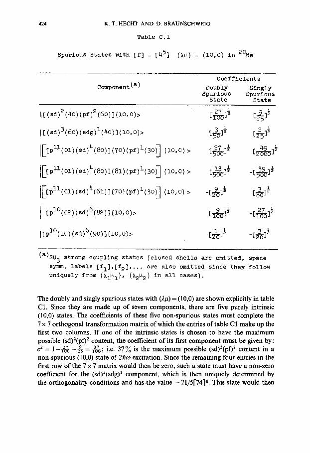
424
Spurious
K. T. HECHT AND D. BRAUNSCHWEIG
Table C.I
States with If] = [4 5 ] (k#) = (lO, O) in 2ONe
Component(at Coefficients
Doubly Singly Spurious Spurious
State State
I[(sd)2(40)(pf)2(60)](10,0)>
][(sd)3(60)(sdg)l(40)](10,0)>
l[[pll(o1)(sd)~(mo)](70)(pf)l(30~ (lO,O)>
l[[pn(ol)(sd)4(80)](Sl)(pf)l(30~ (lO, O) >
I[[pll(ol) (sd)4(,l)](,0~ (pf)l(Bo~ (lO, O) >
[plO(o2)(sd)6(82)](lO, O)>
I[plO(lo)(sd)6(90)](lO, O)>
-c&a
(a)su 3 strong coupling states (closed shells are omitted, space
symm. labels [fl],[f2],... are also omitted since they follow
uniquely from (kl~l), (k2~2) in all cases).
The doubly and singly spurious states with (Z/z) = (10,0) are shown explicitly in table C1. Since they are made up of seven components, there are five purely intrinsic (10,0) states. The coefficients of these five non-spurious states must complete the 7 x 7 orthogonal transformation matrix of which the entries of table C1 make up the first two columns. If one of the intrinsic states is chosen to have the maximum possible (sd)2(pf) 2 content, the coefficient of its first component must be given by: c 2 = 1 - i ~ 0 _ 9 = 1~o; i.e. 37% is the maximum possible (sd)2(pf) 2 content in a non-spurious (10,0) state of 2ho9 excitation. Since the remaining four entries in the first row of the 7 x 7 matrix would then be zero, such a state must have a non-zero coefficient for the (sd)a(sdg) * component, which is then uniquely determined by the orthogonality conditions and has the value -21/5174] ½. This state would then
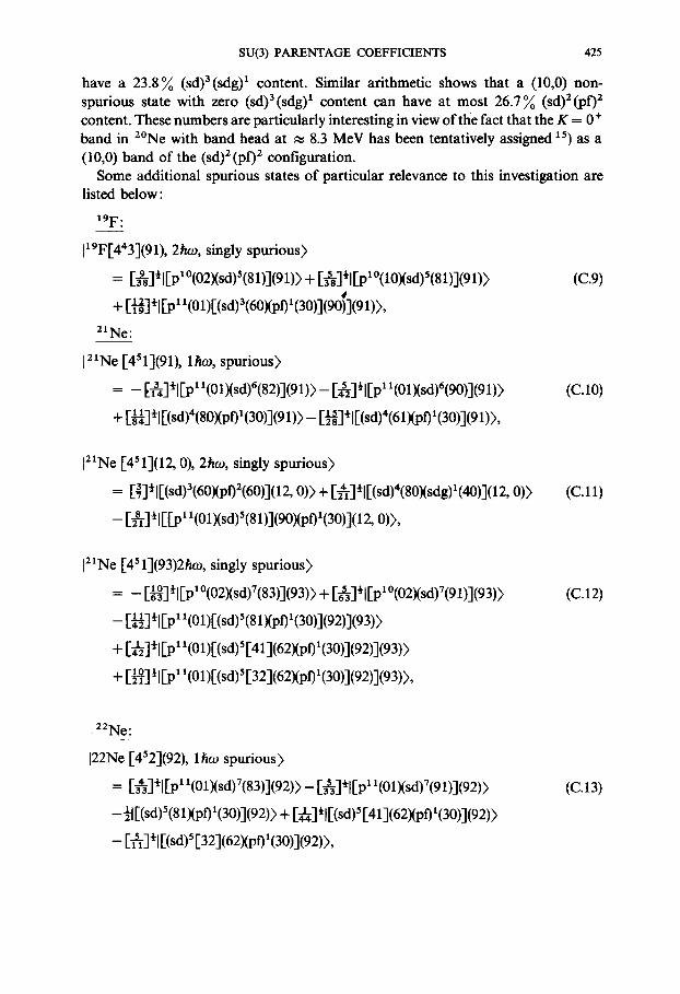
SU(3) PARENTAGE COEFFICIENTS 425
have a 23.8~o (sd)3(sdg) ~ content. Similar arithmetic shows that a (10,0) non- spurious state with zero (sd)3(sdg) 1 content can have at most 26.7~o (sd) 2 (pf)2 content. These numbers are particularly interesting in view oftl ie fact that the K = 0 ÷ band in 2°Ne with band head at ~ 8.3 MeV has been tentatively assigned ~5) as a (10,0) band of the (sd)2(pf) 2 configuration.
Some additional spurious states of particular relevance to this investigation are listed below:
19F:
119F[443](91), 2hto, singly spurious)
= [9 ]~ l [p l °(02Xsd)S(81)](91)) + [~]~l [p l °(10Xsd)5(81)](91)) (C.9)
+ [~]~l [p x l(01)[(sd)a(60Xpf)*(30)](90)](91)),
21Ne:
121Ne [451](91), lhco, spurious)
= - [ ~ ] ~l[p 11(01Xsd)6(82)](91) ) - [~2] ~I[P 11 (01Xsd)6(90)] (91 ))
+ [~]~}l[(sd)4(80)(pI) 1(30)] (91) ) - [ ~ ] *l[(sd)4(61 )(pf) 1(30)] (91 )),
(C.10)
121Ne [451](12, 0), 2hto, singly spurious)
= [a]~l[(sd)a(60)(pf)2(60)](12, 0 ) ) + [~]~l[(sd)'(80)(sdg)l(40)](12, 0))
- [~]*[[[p~ l(01Xsd)5(81)](90)(pf)l(30)](12, 0)),
(C.11)
[2tNe [4Sl](93)2hto, singly spurious)
= _ [~]~l[p 1°(02)(sd)7(83)](93)) + [~]~l[p I °(02)(sd)7(91)](93))
- [~2]~l[p 11(01)[(sd)5(81)(pf)1(30)](92)](93))
+ [~-2] ½liP 11 (01 ) [(sd) 5 [41] (62Xpt) 1 (30)] (92)] (93) )
+ [~]½l[p 1 l(O1)[(sd)S[32](62)(pt)X(30)](92)](93)),
(C.12)
22Ne:
122Ne [452](92), 1 ho9 spurious)
= [~-3]~[[p 1 l(01Xsd)7(83)](92)) - 1~]½[[p 11(01)(sd)7(91)](92))
- ½1[(sd)5(81Xpf)l(30)](92)) + [~]*[[(sd) 5 [41](62Xpf) l(30)](92))
- [~]~l[(sd)S [32](62)(pt) 1 (30)](92)),
(C.13)
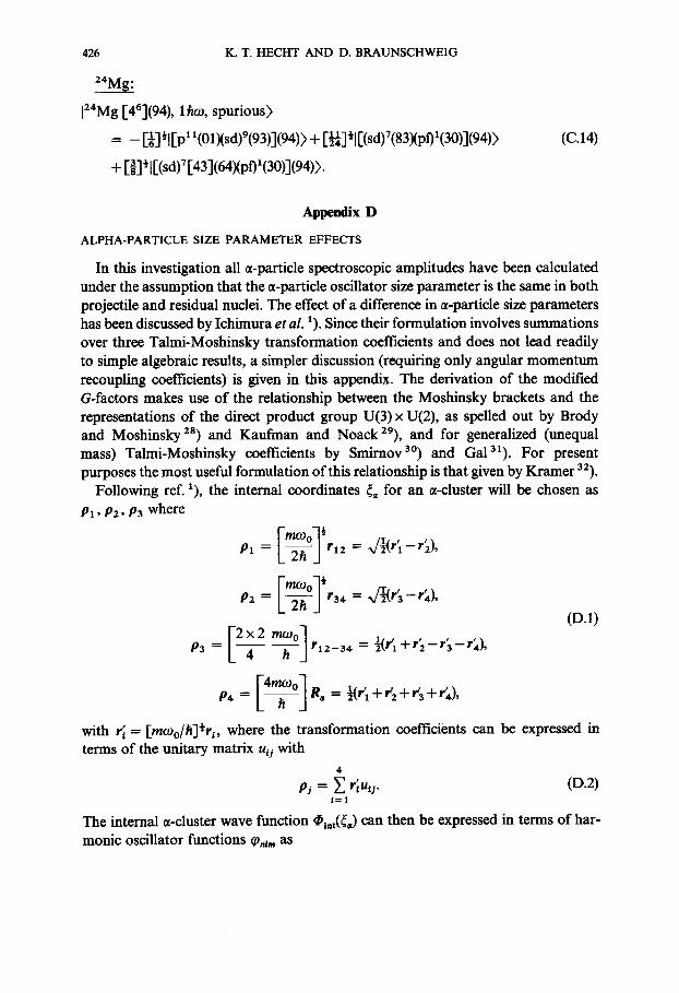
426 K.T. HECHT AND D. BRAUNSCHWEIG
24Mg:
]24Mg [46](94), 1 hoJ, spurious)
= _ [}]½1[p 1 t(O1Xsd)9(93)](94))+ [~]½1[(sd)7(S3Xpt)1(30)](94))
+ []]~l[(sd)7143](64)(pt)1(30)](94)).
(C.14)
Appendix D
ALPHA-PARTICLE SIZE PARAMETER EFFECTS
In this investigation all u-particle spectroscopic amplitudes have been calculated under the assumption that the u-particle oscillator size parameter is the same in both projectile and residual nuclei. The effect of a difference in u-particie size parameters has been discussed by Ichimura et al. 1). Since their formulation involves summations over three Talmi-Moshinsky transformation coefficients and does not lead readily to simple algebraic results, a simpler discussion (requiring only angular momentum recoupling coefficients) is given in this appendix. The derivation of the modified G-factors makes use of the relationship between the Moshinsky brackets and the representations of the direct product group U(3)x U(2), as spelled out by Brody and Moshinsky 28) and Kaufman and Noack29), and for generalized (unequal mass) Talmi-Moshinsky coefficients by Smirnov 3°) and Ga131). For present purposes the most useful formulation of this relationship is that given by Kramer 32).
Following ref. 1), the internal coordinates ~ for an u-cluster will be chosen as
P l , P2, P3 where
I -~O]½r
_ -
(D.1) --[: 2 2 o. r12-34 P3 = "~(/d1-1- r2 -- r3 -- r4),
p,t = [ ~ ] R ~ = 21(r ' l+rt2+d3+r4),
with r~ = [mtOo/h]~r i, where the transformation coefficients can be expressed in terms of the unitary matrix u u with
4- Pj = E r;Uij" (D.2)
/=1
The internal u-cluster wave function Oint(~) can then be expressed in terms of har- monic oscillator functions ~p,~, as
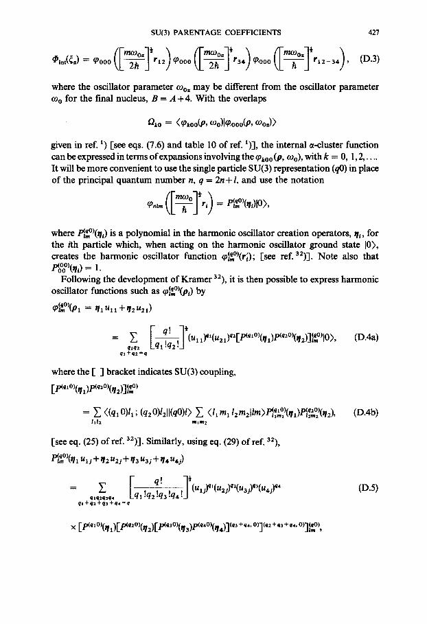
SU(3) PARENTAGE COEFFICIENTS 427
@in*(L) = ‘PO00 ([yk,) ‘pooo ([ypyr34) ‘pooo ([yJ$2-3J 9 (D.3)
where the oscillator parameter uoa may be different from the oscillator parameter o. for the final nucleus, B = A +4. With the overlaps
%o = (%OO@, ~o)l~ooo@9 woJ>
given in ref. ‘) [see eqs. (7.6) and table 10 of ref. ‘)I, the internal cr-cluster function can be expressed in terms of expansions involving the qroo(P, wo), with k = 0, 1,2,. . . .
It will be more convenient to use the single particle SU(3) representation (@) in place of the principal quantum number n, q = 2n+l, and use the notation
-0 +
cp ~ nlm ([ I> h ri = ~‘(rti)l”>~
where P$~op’(sJ is a polynomial in the harmonic oscillator creation operators, vi, for the ith particle which, when acting on the harmonic oscillator ground state IO), creates the harmonic oscillator function (pgop’ (r;); [see ref. 32)]. Note also that pbooo’(~,) = 1.
Following the development of Kramer “), it is then possible to express harmonic oscillator functions such as (P$,~)&) by
cplilO’(P, = ~1~1,+rlz%,)
where the [ ] bracket indicates SU(3) coupling,
[P(q10)(ql)P(q20)(12)]j~)
[see eq. (25) of ref. 32)]. Similarly, using eq. (29) of ref. 32),
~~oP)(rllulj+q2u2j+l13u3j+e4u4j>
= = [ 41
q! tcu,j)yu2j)yu3j)yu4j)~~ 41424394 !q2 !q3 !a! 1 41+42+43+44=4 (D-5)
428 K.T. HECHT AND D. BRAUNSCHWEIG
so that, for example
~0000 ( [ - - - ~ ] ½ J P 1 2 - 3 4 . ) = {~'~00 "~ lf~10(P(02°)(~1) "~" P(go°)(,2) ='[= P(20°)(I~3) -~- P(oo°)(~4.))
1 ! 10) 10) (20) 10) 10) (20) +~,,/~alO([e~ (,t,).~ (,t2)]oo + [ ~ (~)-~ (~,)]oo) 1 10) 10) (20) 10) 10) (20) 10) 10) (20)
-- '2X/~Q10([ P ( ( 1 1 1 ) P( (~3)]00 " ~ - [ e ( ( i 1 1 ) P( (174)]00 "~- [ e ( (112) P( (I]4)]00
4- [P(I°)(q2)P(I°)(II3)](2°))-F terms of order 020 +...}10), (D.6)
and the internal g-cluster function of eq. (D.3) becomes 4 4
y~3 _1. 3~,-~2 ~ ~ p(20)(. "~ 1 /1-(')2 (') Fp( lo) t . ~p(lO)/. ~'1(20) (~int(~cz) / 0 0 " 4 00 10 / , - - 0 0 I- '/ i/-- '2\ 2 " 0 0 " 1 0 E L ~ ~ ' l tP t V ' I j I J O 0
i = 1 i < j = 1
+terms of order (g2oof~12o, fto2of22o)+ ...}10). (D.7)
~(Qo)~p,~ for the Eq. (D.5) when applied to the function Cm.u([4mOgo/h]½R=)=_ = , . u ~..,J
c.m. motion of the ~-cluster yields
¢(eo)tw, ~ [ q Q ' ] ½ 1 /.M ~,"=y ---- qta2e,e, I tq2 [q3 !q4 i -2 ~
qt +q2+q3+q4=Q
qlO) q20) q30) q40) (q3+114 O) (q2+~/3+1/4 x [ P( (~/1)C P( (~/2)[ P( (q3) P( (~/4)] ' ] ,o)l(Qo)n\jr.u v/, (D.8)
which together with eq. (D.7) shows that the G-factor of eq. (3) of the text, with Q = 2 N + L = ~q~, must be modified by the factor t2o3o . To first order in t21o G- factors for Q = 2N+ L = ~q~-2 are also different from zero. For this case, with Q = 6 for example
¢(6o),p,~ f[ 6! ]½ 1 p(6o) p(6o) _[_p(6o)
I-6!] ' I } + P~) (~ ~2 ~))+ [ ~ j ~ (/~N)(~x ~2; ~ ~4) + 5 similar terms)+... I0), (D.9)
where
I-p(20){,~ hI-D(20)l,m hD(20)(,~ h-1(40)'](60) P(6M0)(I'/2~3~4)------L-- I.°12/L-- V'I3'-- ~,'la..,J J L M '
10) 10) (20) 20) 20) (4.0) (60) ~6o),.,,.,,.,1.,2... ,h,t,) -= [ [~ (,h)~ (,h)] [ ~ (,h)~ (,I.)] ]L,.,.
and where the terms denoted by ... involve particles in the (30), (40),... shells. There are then only two types of terms in the product ~int(~)~(L~)(R~) which can give non-zero contributions to the overlap with the four-particle shell model function for the configuration (ls0d)4:
(I) Four terms of the type
SU(3) PARENTAGE COEFFICIENTS 429
~go °)(~l)P£~)t~2 ~3 ~,)
--- E ((20)0; (60)Cll(,lU)~C>E~2°~(~0[~°)(~2)E~2°)(,h)~2°)(~,)]('°)](6°)]~g~, (D.10)
(II) Six terms of the type
20) 10) (20) 60) • [t~o (,t,)~ (+2)]oo ~gM(+l+2, +3+4)= ~ <(20)0; (60)t, ll(,l~)~L>E[~x°)(,h) O.~)r
D(10)/. ~-1(20)['['D(10)(~ ~D(10)(. ~1(20)['D(20)[. "t]D(20)(. ~"](40)-[(60)'1(2/0 (D.11) ) ~t 1,121j LL ~ ~'11] ~ ~'121J L z ~ '13, f~ ~'14]1 J J~:LM"
The term singled out in (D. 10) is in a form convenient for a parentage expansion in which the (ls0d) particle labeled 1 is coupled to a totally symmetric group of three (ls0d) particles. Some recoupling is required to get the remaining three terms of this type into this form. For example
i-p(20)(,, ~ p ( 6 0 ) ( . . . . , )l(,~) = [p(20!(q2)[pt20)(ql)P(40)(~13n,]l(60)l(2~) -#41A d r L M L ~,r121 I l l ~13 "14 J~cLM
= ~ U((20)(20)(2#~(40); (~#)(60))(-1)4+~+~U((20)(20)(2#)(40); (~-/~X2'#')) (~(~'~')
r ~ o ) / . ~rpt20)t., ~p(40)l,, . , ~-1(60)-1(2~a) (D.12) X L ~ ~" ~ I I I L a ~,~121 a ~,~13~141J J~cLM,
where an interchange in the order ofp(2°)(~/1), P(2°)(q2) in the SU(3) Wigner coupling [P(2°)(l]2)P(2°)(~]l)](x~ has been sandwiched in between the two 6-(2/~) recoupling transformations. Since all SU(3) representations in both types of SU(3) U-coef- ficients are at most two-rowed, these can be replaced by SU(2) (ordinary angular momentum) Racah coefficients in unitary form; e.g.
u((20X20X~.X40); (~gX60)) = u 11 ~ 2; ~ 3 .
Also, ( - I I ~'÷~ = ( - 1)½~'; so that a composition of ordinary angular momentum recoupling coefficients can be used to express (D. 12) in the form
E P t 2 ° ) ( q 2 ) P t 6 ° ) ( q l ~ I a q 4 ) ] ~ M = Z U ( 1 2 ' ~ ( ~ ' W ) ~ 1; 3 ~ ) ( - 1) ½x+t~''+3
X [P(2 °)(~/1 ) [P(2 °)(~/2 )[P(2 °)(~/3)P(2°)(q4)] (4°)] (A'/~')](~c~'ff)M . (D.13)
Using similar recoupling transformations on the last two terms of type (D.10) the sum over the four terms of this type yields
4 ~_, p~2o°)(qi)P~6~)(tl i qk q,)
i=1 ( j<k<I f : i )
= 4<(20)0; (60)Ll[(80)L>Ep(2°)(qOEP~2°)(~12)EP(2°)(qa)Pt2°)(~h)]('~°)-l(6°)]~La°) _6- 20) 20) 20) 20) (40) (60) (42) +((20)O;(60)LII(42)rL>{n[/~ Oh)[/~ 0/2)[ P~ (~h) -p( 0/4)] ] ],,,.u
+ ~ 3333~[~2°)(~,)[~2°)(~X~[~2°)(~)~2°)(~,)]('°)
+ ½x/~[P(2°)(~/a)p(2°)(~14)l(°2))l(22)l~}. (D.14)

430 K . T . H E C H T A N D D. B R A U N S C H W E I G
Terms of type (D. 11) involve somewhat more recoupling. Using
!- 2* 7½ L - - ~'111-- t ' l l JJ l ra = lm ( q l )
[see eqs. (10) to (15) of ref. 3 2 ) ] , and simple SU(3) recoupling transformations
( 2 ~ ) ( ! ½ IX) ( 2 _ 2 . ~ ) - -2 Z Z U 11 i2 ; 3 X ½ 1 U 11 (~,)(x'u') X 1 ½ 2 '
X Lre(2°)i'XOll/L~rp(2°)t'w2 )rp(2o)(.L "13 )~20)t.~,14 ) l (40) l (2 '~ ' ) l (z" ) , 3 / I r L M
(D.15)
(D.16)
where we have used
/(10) (10) (20)~ t ½1t Xsu(a)/(10 ) (10) ( 20 ) /= X ½ 1
k,(20) (20) (~fi)/ 1 ½~-j (D.17)
to replace an SU(3) 9-(2#) coefficient in which all SU(3) representations are at most two-rowed by an ordinary angular momentum 9-j coefficient (the X-coefficient or the unitary form of the 9-j coefficient), with similar replacements for two SU(3) U- coefficients in which all representations are again at most two-rowed. The sum of the six terms of type (D.11) then yields
4 rp ( lo ) t , , ~p(lO)(~ ~-l(20)D(60)(~ ~ . L-- I,'$i/-- ~,'ljlJO0 - - L M ~, ' l i ' l j , ~k~l )
i < j = l (k<l: . - / : i , j )
20) 20) (20) 20) (4.0) (60) (A#) = ~((20)O(60)LII().I~)xL)[ t~ (gx)[ P~ (i/2)[P (//3)/:~ (1'/4.)] ] ]KLM (,;tu)
x (126(a.)(so) - 2t~(xu)(42) ). (D.18)
Note that terms with three-particle representations (2'/1') = (22) are missing even though they are allowed both by the coupling rules and by symmetry. The coefficient of this term is zero through cancellation of terms with different X in the sum of eq. (D.16).
Finally, to calculate the overlap (60) l [41(2/4) 4 ~ t ~
( ~ i n t ( ~ a ) ~ i L M (R,)[~LM ((ls0d) , r 1 r 2 r 3 r4)) = G(6°)((ls0d)4[4](A/0xL), (D.19)
the G-factor with 2 N + L = 6 for ~-particles of proper size, a parentage expansion of the (1 s0d) 4 particle shell model wave function is used
(20) 20) (20) (20) (40) (60) (80) --LMmt4l(SO)t",'X'2"' "a" "4,/" ~\ = I[P (th)[P ( 0/2)['P 0/3)P (I/4 ] ] ]LM 10), (D.20a)
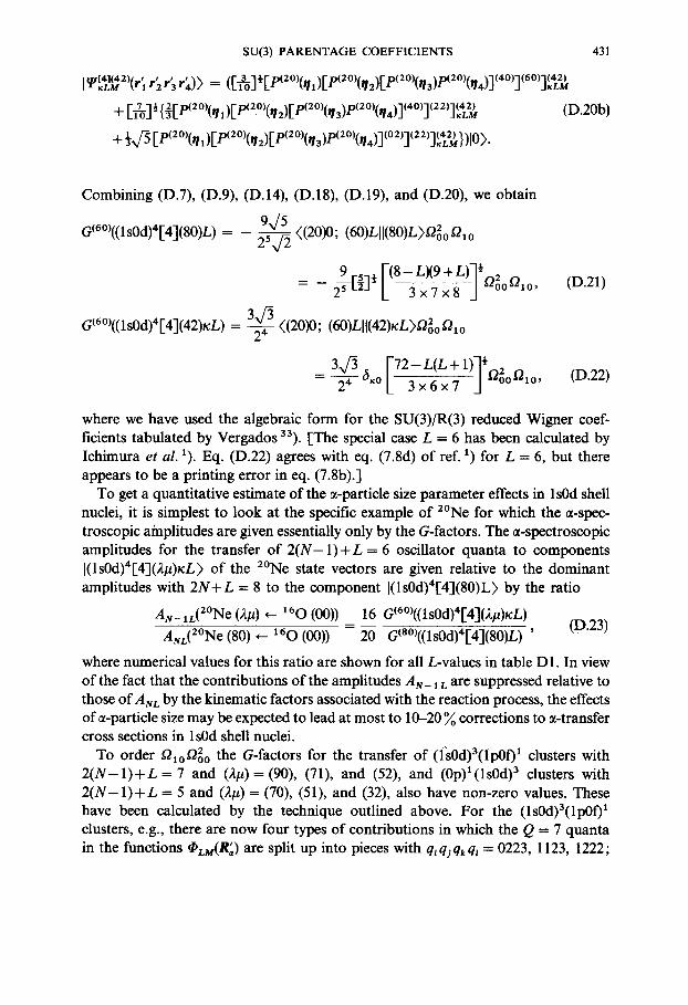
SU(3) P A R E N T A G E COEFFICIENTS 431
t//[4](42)(s.' ~.' F' ~.' SX ([" 3 l~[ 'p(20)(~ ~ro(20)(.. xrp(20)(.. ~p(20)(.. ~'](40)1(60)1(42) K L M ~ , ' 1 " 2 ~ ' 3 " 4 1 / = ~.LT'6.J L - - ~ , ' I I I L Jt 1? /2 /LJ t ~'131 "t ~'141J I I r L M
"~- LIojF----7 l½ f--2 ['P(20)G"L3L t'IlIL~Fp(20)t"~q21L~Fp(20)t'~'f3 )p(2O)(..,i,~ )'](40)](22)](42) J d 3gLM (D.20b)
l 20) (20) 20) 20) (02) (22) (42) +745[P( Oh)[ P (I/2)[ P((q3) P( 0/4)] ] ],LM})[O>.
Combining (D.7), (D.9), (D.14), (D.18), (D.19), and (D.20), we obtain
945 a(6°)((ls0d)a[a](80)L) = 25x/~ ((20)0; (60)LIl(80)L)t22ot21o
9 I-(8 - L)(9 + L)-I ~ 2 - 2, / 1 000010, (D.21)
G(6°)((ls0d)414](42)xL) = ~ ((20)0; (60)LIl(42)xL>t220 t21o
34524 dixo L_ [ 7 2 - L(L3xgx7 + 1)] ½t22° f21°' (D.22)
where we have used the algebraic form for the SU(3)/R(3) reduced Wigner coef- ficients tabulated by Vergados 33). [ -The special case L = 6 has been calculated by Ichimura et al. 1). Eq. (D.22) agrees with eq. (7.8d) of ref. 1) for L = 6, but there appears to be a printing error in eq. (7.8b).]
To get a quantitative estimate of the ~t-particle size parameter effects in 1 sOd shell nuclei, it is simplest to look at the specific example of 2°Ne for which the ~t-spec- troscopic a/nplitudes are given essentially only by the G-factors. The ~-spectroscopic amplitudes for the transfer of 2 ( N - 1 ) + L = 6 oscillator quanta to components I(ls0d)4[4](2#)rL> of the 2°Ne state vectors are given relative to the dominant amplitudes with 2N+ L = 8 to the component I(1 s0d)414](80)L> by the ratio
A s _ 1L(2°Ne (2#) ~ 160 (00)) 16 G(6°)((lsOd)4[4](2#)xL)
ANL(2°Ne (80) ~ 160 (00)) = 20 G(a°)((ls0d)'[4](80)L) ' (9.23)
where numerical values for this ratio are shown for all L-values in table D1. In view of the fact that the contributions of the amplitudes A N_ 1 r. are suppressed relative to those o f AuL by the kinematic factors associated with the reaction process, the effects of ~-particle size may be expected to lead at most to 10-20 ~o corrections to ~t-transfer cross sections in 1 sOd shell nuclei.
To order 010020 the G-factors for the transfer of (ls0d)a(lp0f) 1 clusters with 2 ( N - 1 ) + L = 7 and (2/~)= (90), (71), and (52), and (0p)l(ls0d) 3 clusters with 2 ( N - 1 ) + L = 5 and (2#)= (70), (51), and (32), also have non-zero values. These have been calculated by the technique outlined above. For the (ls0d)3(lp0f) 1 clusters, e.g., there are now four types of contributions in which the Q = 7 quanta in the functions ~Lu(R~) are split up into pieces with q~ qj qk q~ = 0223, 1123, 1222;
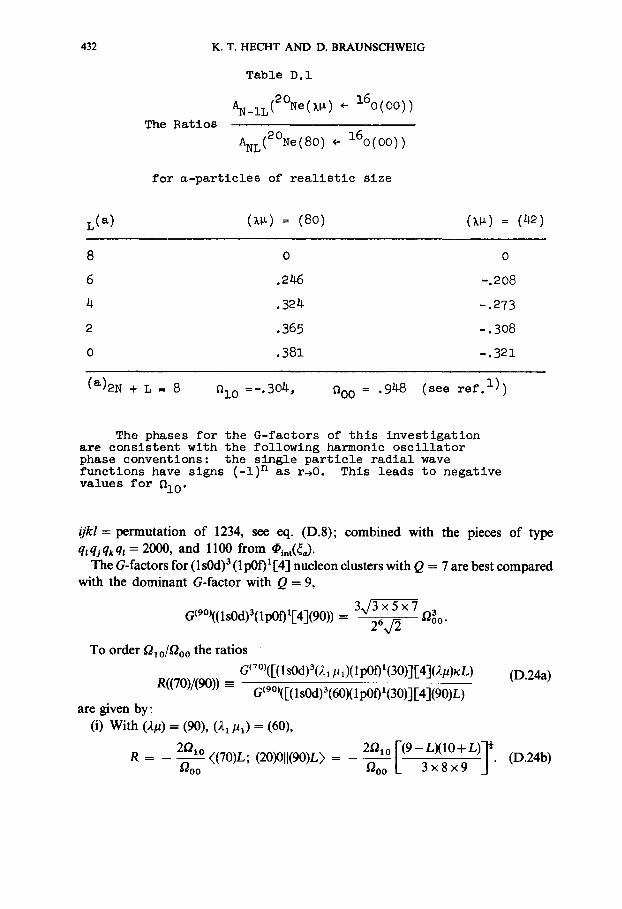
432
The Ratios
K. T. HECHT AND D. BRAUNSCHWEIG
Tab le D. 1
AN_IL(2ONe(Mz) <- 160(00))
ANL(2ONe(80) 4- 160(00))
for a-particles of realistic size
z(a) (x~) = (8o) (x~) = (42)
8 0 0
6 .246 -.208
4 .324 -.273
2 .365 -.308
0 .381 -.321
(a)2N + L = 8 010 =-.304, O00 = .948 (see ref. I))
The phases for the G-factors of this investigation are consistent with the following harmonic oscillator phase conventions: the single particle radial wave functions have signs (-1) n as r,0. This leads to negative values for Ol0"
ijkl = permutation of 1234, see eq. (D.8); combined with the pieces of type q~qjqkql = 2000, and 1100 from ~i.t(~).
The G-factors for (1 s0d) 3 (lp0t)* I-4] nucleon clusters with Q = 7 are best compared with the dominant G-factor with Q = 9,
G(9O)((1 s0d)3( 1 p0f) 114](90)) -
To order Olo/Ooo the ratios
3 x / 3 x 5 x 7 °o o •
G t 7 o)( [(1 sOd) 3 (21 #1)(1 p0f) 1(30)] [4](2#)xL)
R((70)/(90)) - Gt9O,([(ls0d)a(60X lp0f) x (30)] [4](90)L) are given by:
(i) With (,~]~) = (90), (,~1/~i) = (60),
2OlO [ ! 9 - LXIO+ L ) I ' R = 20*° <(70)L; (20)011(90)L) = - - - 0oo 0oo L 3 x 8 x 9 J "
(D.24a)
(D.24b)
SU(3) PARENTAGE COEFFICIENTS 433
(ii) With (2#) = (71), (2 x/q) = (60),
2 t21o ((70)L; (20)0[[(71)L) = 2 axo FEL( L + 1)]* R = x/~ Ooo ~ooL 27 _]" (D.24c)
(iii) With (2#) = (52), (21/~1) = (60), t , ' ,
4x/3 t2,o F_98 - L(L-I- 1)]½ 4x/~ 12'° ((70)L; (20)011(52)xL) x / ~ t~oo L 3 × 7 × 8 _1 " R = x/r~ t2o~ = - - - - 6,o (D.24d)
(iv) With (2#) = (52), (21 $q) = (22),
8 4,o 8 a,o 78-w,+1)? R = 3 7 t2oo ((70)Z; (20)011(52)rL) = 3x/3 t2oo .o I_ 3 × 7 × 8 _1 " (D.24e)
Similarly, the G-factors for (0p)l(ls0d) 3 [4] nucleon clusters with Q = 5 are best expressed in terms of the ratios
R((50)/(70)) = GtS°)([(OP)X(lO)(lsOd)a(221~2)][4](21g)xL) GtTO)([(0p)~ (10X1 s0d)3(60)] [4](70)L) , (D.25a)
where (i) with (2#) = (70), (22/~2) = (60),
~ o 3t21o [-_3 (7-LX8 + L!-] ½ R = -3x/~7 v v ((50)L; (20)011(70)L) = ~ L 7 3 x 6 x 7 J ' (D.25b)
(ii) with (2#) = (51), (22 #2) = (60),
" I2~° [2L(L+ 1)1½, (D.25c) R = ~ 4 I2oot2X° ((50)L; (20)011(51)L) = . . . . 3s t2oo
(iii) with (2$t) = (32), (22 #2) = (22),
R - x/~x 7 --i2oo ((50)L; (20)011(32)xL) = 4t2~Ot2o____~ 6x 7 [ 5 0 - L ( L + 1 ) ] 3 ~ x 6 ½°°~°iD.25d )
For all L-values the ratios of eqs. (D.24) and (D.25) have magnitudes comparable to the illustrative numbers of table D1.
Finally, G-factors for I-x] nucleon clusters with x ~ 4 can be calculated by similar techniques. For a three-nucleon cluster, e.g., the internal and c.m. coordinates Pl, P2, R~ can be chosen as
Fmcool ½ "01 = L -J r,2 =
[132 mCOo-l' P2 = - ~ - j r,2_ 3 = x/~g(r'a+r~-2r~), (D.26)
[-3m~Oo-1½
434 K.T. HECHT AND D. BRAUNSCHWEIG
in the notation of eq. (D. 1). For three-nucleon clusters with oscillator size parameter [mcoo/h]½; i.e. with COo3 = COo, eq. (D.5) then leads at once to the G-factor given by eq. (4) of the text.
References
1) M. Ichimura, A. Arima, E. C. Halbert and T, Terasawa, Nucl. Phys. A204 (1973) 225 2) D. Kurath and I. S. Towner, Nucl. Phys. A222 (1974) 1 3) J. P. Draayer, Nucl. Phys. A237 (1975) 157 4) B. Buck, C. B. Dover and J. P. Vary, Bull. Am. Phys. Soc. 18 (1973) 1414, and to be published 5) N. Takigawa and A. Arima, Nucl. Phys. A168 (1971) 593;
N. De Takacsy and S. DasGupta, Phys. Lett. 33B (1970) 556 6) N. Anyas-Weiss, J. C. Cornell, P. S. Fisher, P. N. Hudson, A. Menchaca-Rocha, D. J. Millener,
A. D. Panagiotou, D. K. Scott, D. Strottman, D. M. Brink, B. Buck, P. J. Ellis and T. Engeland, Phys. Reports 12C (1974) 201
7) Y. Akiyama and J. P. Draayer, Computer Phys. Commun. 5 (1973) 405 8) J. P. Draayer and Y. Akiyama, J. Math. Phys. 14 (1973) 1904 9) A. Arima, H. Horiuchi and T. Sebe, Phys. Lett. 24B (1967) 129
10) P. J. Ellis and T. Engeland, Nucl. Phys. A144 (1970) 161 ; Alg l (1972) 368 11) S. Lie, T. Engeland and G. Dalai, Nucl. Phys. A156 (1970) 449; A169 (1971) 617 12) A. Arima and D. Strottman, Nucl. Phys. A162 (1971) 423, 605 13) M. Harvey, Nucl. Phys. A202 (1973) 191 14) K. T. Hecht, Nucl. Phys. A170 (1971) 34 15) H. T. Fortune, Argonne Physics Division, Informal Report PHY-1973B, March 1973 16) Y. Akiyama, Nucl. Data A2 (1967) 403 17) K. T. Hecht and S. C. Pang, J. Math. Phys. 10 (1969) 1571 18) D. Kurath, Phys. Rev. C7 (1973) 1390 19) R. T. Sharp, H. C. von Baeyer and S. C. Pieper, Nucl. Phys. A127 (1969) 513 20) M. Harvey and F. C. Khanna, Nuclear spectroscopy liB, ed. J. Cerny and G. Ripka; in Advances
in nuclear physics, vol. 1, ed. E. W. Vogt and M. Baranger (Plenum, New York, 1968) 21) M. Harvey, in Advances in nuclear physics, vol. 1, ed. E. W. Vogt and M. Baranger (Plenum, New
York, 1968) 22) L. C. Biedenharn, J. D. Louck, E. Chacon and M. Ciftan, J. Math. Phys. 13 (1972) 1957 23) J. P. Bernier and M. Harvey, Nucl. Phys. A94 (1967) 593 24) A. Arima and D. Strottman, A compilation of SU(3) wave functions, Nuclear Physics Theoretical
Group Report no. 46, Nuclear Physics Laboratory, Oxford University, ref. 14/73 25) A. VanderMolen, J. Janecke and F. D. Beeehetti, Bull. Am. Phys. Soc. 19 (1974) 989; also private
communication 26) Y. Akiyama, Nucl. Data A2 (1967) 403 27) H. A. Jahn and H. van Wieringen, Proc. Roy. Soc. A209 (1951) 502 28) T. A. Brody and M. Moshinsky, Rev. Mex. de Fis. 9 (1960) 181 29) B. Kaufman and C. Noack, J. Math. Phys. 6 (1965) 142 30) Yu F. Smirnov, Nucl. Phys. 27 (1961) 177; 39 (1962) 346 31) A. Gal, Ann. of Phys. 49 (1968) 341 32) P. Kramer, Rev. Mex. de Fis. 19 (1970) 241 33) J. D. Vergados, Nucl. Phys. A l l l (1968) 681