Embed Size (px)
Citation preview
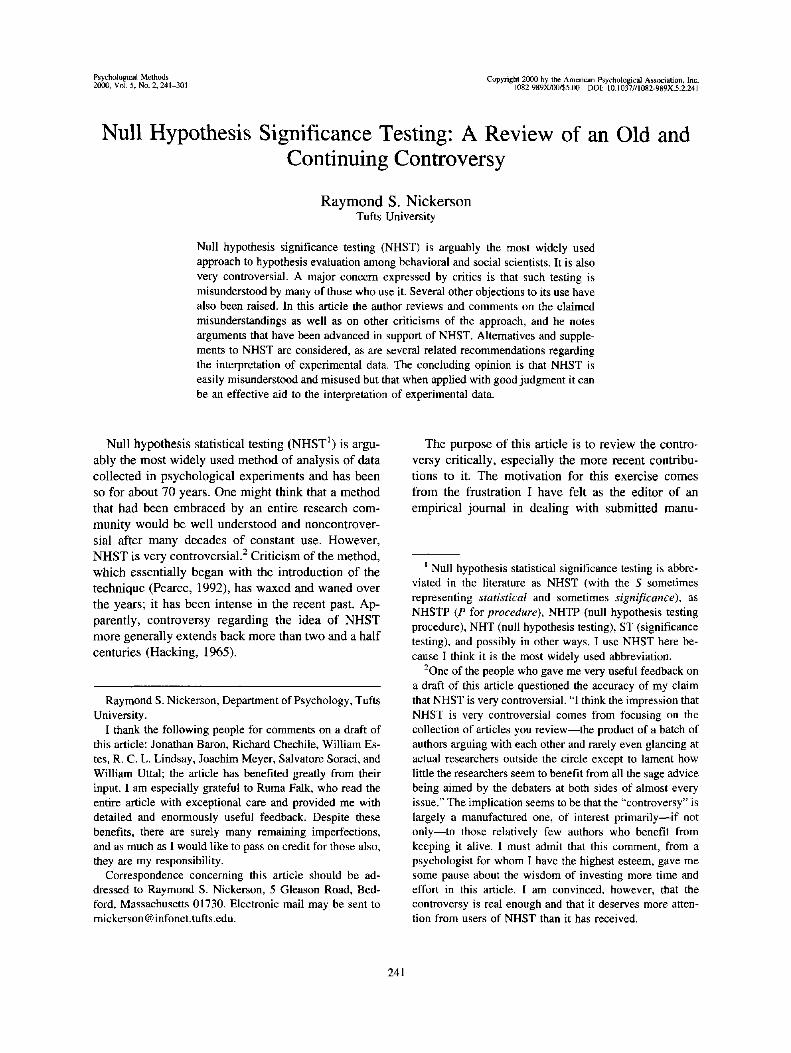
Psychological Methods2000, Vol.5, No. 2,241-301
Copyright 2000 by the American Psychological Association, Inc.I082-989X/00/$5.00 DOI: I0.1037//1082-989X.S.2.241
Null Hypothesis Significance Testing: A Review of an Old andContinuing Controversy
Raymond S. NickersonTufts University
Null hypothesis significance testing (NHST) is arguably the mosl widely used
approach to hypothesis evaluation among behavioral and social scientists. It is also
very controversial. A major concern expressed by critics is that such testing is
misunderstood by many of those who use it. Several other objections to its use have
also been raised. In this article the author reviews and comments on the claimed
misunderstandings as well as on other criticisms of the approach, and he notes
arguments that have been advanced in support of NHST. Alternatives and supple-
ments to NHST are considered, as are several related recommendations regarding
the interpretation of experimental data. The concluding opinion is that NHST is
easily misunderstood and misused but that when applied with good judgment it can
be an effective aid to the interpretation of experimental data.
Null hypothesis statistical testing (NHST1) is argu-
ably the most widely used method of analysis of data
collected in psychological experiments and has been
so for about 70 years. One might think that a method
that had been embraced by an entire research com-
munity would be well understood and noncontrover-
sial after many decades of constant use. However,
NHST is very controversial.2 Criticism of the method,
which essentially began with the introduction of the
technique (Pearce, 1992), has waxed and waned over
the years; it has been intense in the recent past. Ap-
parently, controversy regarding the idea of NHST
more generally extends back more than two and a half
centuries (Hacking, 1965).
Raymond S. Nickerson, Department of Psychology, Tufts
University.
I thank the following people for comments on a draft of
this article: Jonathan Baron, Richard Chechile, William Es-
tes, R. C. L. Lindsay, Joachim Meyer, Salvatore Soraci, and
William Uttal; the article has benefited greatly from their
input. I am especially grateful to Ruma Falk, who read the
entire article with exceptional care and provided me with
detailed and enormously useful feedback. Despite these
benefits, there are surely many remaining imperfections,
and as much as I would like to pass on credit for those also,they are my responsibility.
Correspondence concerning this article should be ad-
dressed to Raymond S. Nickerson, 5 Gleason Road, Bed-
ford, Massachusetts 01730. Electronic mail may be sent to
The purpose of this article is to review the contro-
versy critically, especially the more recent contribu-
tions to it. The motivation for this exercise comes
from the frustration I have felt as the editor of an
empirical journal in dealing with submitted manu-
' Null hypothesis statistical significance testing is abbre-
viated in the literature as NHST (with the 5 sometimes
representing statistical and sometimes significance), as
NHSTP (P for procedure), NHTP (null hypothesis testing
procedure), NHT (null hypothesis testing), ST (significance
testing), and possibly in other ways. I use NHST here be-
cause I think it is the most widely used abbreviation.2One of the people who gave me very useful feedback on
a draft of this article questioned the accuracy of my claim
that NHST is very controversial. "I think the impression that
NHST is very controversial comes from focusing on the
collection of articles you review—the product of a batch of
authors arguing with each other and rarely even glancing at
actual researchers outside the circle except to lament how
little the researchers seem to benefit from all the sage advice
being aimed by the debaters at both sides of almost every
issue." The implication seems to be that the "controversy" is
largely a manufactured one, of interest primarily—if not
only—to those relatively few authors who benefit from
keeping it alive. I must admit that this comment, from apsychologist for whom I have the highest esteem, gave me
some pause about the wisdom of investing more time and
effort in this article. I am convinced, however, that the
controversy is real enough and that it deserves more atten-
tion from users of NHST than it has received.
241
242 NICKERSON
scripts, the vast majority of which report the use of
NHST. In attempting to develop a policy that would
help ensure the journal did not publish egregious mis-
uses of this method, I felt it necessary to explore the
controversy more deeply than I otherwise would have
been inclined to do. My intent here is to lay out what
I found and the conclusions to which 1 was led.3
Some Preliminaries
Null hypothesis has been defined in a variety of
ways. The first two of the following definitions are
from mathematics dictionaries, the third from a dic-
tionary of statistical terms, the fourth from a dictio-
nary of psychological terms, the fifth from a statistics
text, and the sixth from a frequently cited journal
article on the subject of NHST:
A particular statistical hypothesis usually specifying thepopulation from which a random sample is assumed tohave been drawn, and which is to be nullified if theevidence from the random sample is unfavorable to thehypothesis, i.e., if the random sample has a low prob-ability under the null hypothesis and a higher one undersome admissible alternative hypothesis. (James &James, 1959, p. 195)
1. The residual hypothesis that cannot be rejected unlessthe test statistic used in the hypothesis testing problemlies in the critical region for a given significance level. 2.in particular, especially in psychology, the hypothesisthat certain observed data are a merely random occur-rence. (Borowski & Borwein, 1991, p. 411)
A particular hypothesis under test, as distinct from thealternative hypotheses which are under consideration.(Kendall & Buckland, 1957)
The logical contradictory of the hypothesis that oneseeks to test. If the null hypothesis can be proved false,its contradictory is thereby proved true. (English & En-glish, 1958, p. 350)
Symbolically, we shall use H0 (standing for null hypoth-esis) for whatever hypothesis we shall want to test andHA for the alternative hypothesis. (Freund, 1962, p. 238)Except in cases of multistage or sequential tests, theacceptance of H0 is equivalent to the rejection of HA, andvice versa, (p. 250)
The null hypothesis states that the experimental groupand the control group are not different with respect to [aspecified property of interest] and that any differencefound between their means is due to sampling fluctua-tion. (Carver, 1978, p. 381)
It is clear from these examples—and more could be
given—that null hypothesis has several connotations.
For present purposes, one distinction is especially im-
portant. Sometimes null hypothesis has the relatively
inclusive meaning of the hypothesis whose nullifica-
tion, by statistical means, would be taken as evidence
in support of a specified alternative hypothesis (e.g.,
the examples from English & English, 1958; Kendall
& Buckland, 1957; and Freund, 1962, above). Of-
ten—perhaps most often—as used in psychological
research, the term is intended to represent the hypoth-
esis of "no difference" between two sets of data with
respect to some parameter, usually their means, or of
"no effect" of an experimental manipulation on the
dependent variable of interest. The quote from Carver
(1978) illustrates this meaning.
Given the former connotation, the null hypothesis
may or may not be a hypothesis of no difference or of
no effect (Bakan, 1966). The distinction between
these connotations is sometimes made by referring to
the second one as the nil null hypothesis or simply the
nil hypothesis; usually the distinction is not made ex-
plicitly, and whether null is to be understood to mean
nil null must be inferred from the context. The dis-
tinction is an important one, especially relative to the
controversy regarding the merits or shortcomings of
NHST inasmuch as criticisms that may be valid when
applied to nil hypothesis testing are not necessarily
valid when directed at null hypothesis testing in the
more general sense.
Application of NHST to the difference between two
means yields a value of p, the theoretical probability
that if two samples of the size of those used had been
drawn at random from the same population, the sta-
tistical test would have yielded a statistic (e.g., t) as
large or larger than the one obtained. A specified sig-
nificance level conventionally designated a (alpha)
serves as a decision criterion, and the null hypothesis
3Since this article was submitted to Psychological Meth-
ods for consideration for publication, the American Psycho-
logical Association's Task Force on Statistical Inference
(TFSI) published a report in the American Psychologist
(Wilkinson & TFSI, 1999) recommending guidelines for the
use of statistics in psychological research. This article was
written independently of the task force and for a different
purpose. Having now read the TFSI report, I like to think
that the present article reviews much of the controversy that
motivated the convening of the TFSI and the preparation of
its report. I find the recommendations in that report very
helpful, and I especially like the admonition not to rely too
much on statistics in interpreting the results of experimentsand to let statistical methods guide and discipline thinking
but not determine it.
NULL HYPOTHESIS SIGNIFICANCE TESTING 243
is rejected only if the value ofp yielded by the test is
not greater than the value of a. If a is set at .05, say,
and a significance test yields a value of p equal to or
less than .05, the null hypothesis is rejected and the
result is said to be statistically significant at that level.
According to most textbooks, the logic of NHST
admits of only two possible decision outcomes: rejec-
tion (at a specified significance level) of the hypoth-
esis of no difference, and failure to reject this hypoth-
esis (at that level). Given the latter outcome, one is
justified in saying only that a significant difference
was not found; one does not have a basis for conclud-
ing that the null hypothesis is true (that the samples
were drawn from the same population with respect to
the variable of interest). Inasmuch as the null hypoth-
esis may be either true or false and it may either be
rejected or fail to be rejected, any given instance of
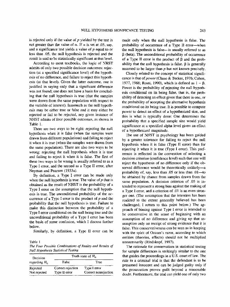
NHST admits of four possible outcomes, as shown in
Table 1.
There are two ways to be right: rejecting the null
hypothesis when it is false (when the samples were
drawn from different populations) and failing to reject
it when it is true (when the samples were drawn from
the same population). There are also two ways to be
wrong: rejecting the null hypothesis when it is true
and failing to reject it when it is false. The first of
these two ways to be wrong is usually referred to as a
Type I error, and the second as a Type II error, after
Neyman and Pearson (1933a).
By definition, a Type I error can be made only
when the null hypothesis is true. The value ofp that is
obtained as the result of NHST is the probability of a
Type I error on the assumption that the null hypoth-
esis is true. The unconditional probability of the oc-
currence of a Type I error is the product ofp and the
probability that the null hypothesis is true. Failure to
make this distinction between the probability of a
Type I error conditional on the null being true and the
unconditional probability of a Type I error has been
the basis of some confusion, which I discuss further
below.
Similarly, by definition, a Type II error can be
Table 1
The Four Possible Combinations of Reality and Results of
Null Hypothesis Statistical Testing
Decision
regarding H0
Truth state of
False True
Rejected Correct rejection Type I error
Not rejected Type 11 error Correct nonrejection
made only when the null hypothesis is false. The
probability of occurrence of a Type II error—when
the null hypothesis is false—is usually referred to as
p (beta). The unconditional probability of occurrence
of a Type II error is the product of p and the prob-
ability that the null hypothesis is false, p is generally
assumed to be larger than p but not known precisely.
Closely related to the concept of statistical signifi-
cance is that of power (Chase & Tucker, 1976; Cohen,
1977, 1988; Rossi, 1990), which is defined as 1 - p.
Power is the probability of rejecting the null hypoth-
esis conditional on its being false, that is, the prob-
ability of detecting an effect given that there is one, or
the probability of accepting the alternative hypothesis
conditional on its being true. It is possible to compute
power to detect an effect of a hypothesized size, and
this is what is typically done: One determines the
probability that a specified sample size would yield
significance at a specified alpha level given an effect
of a hypothesized magnitude.
The use of NHST in psychology has been guided
by a greater tolerance for failing to reject the null
hypothesis when it is false (Type II error) than for
rejecting it when it is true (Type I error). This pref-
erence is reflected in the convention of selecting a
decision criterion (confidence level) such that one will
reject the hypothesis of no difference only if the ob-
served difference would be theoretically unlikely—a
probability of, say, less than .05 or less than .01—to
be obtained by chance from samples drawn from the
same population. A decision criterion of .05 is in-
tended to represent a strong bias against the making of
a Type I error, and a criterion of .01 is an even stron-
ger one. (The assumption that the intention has been
realized to the extent generally believed has been
challenged; I return to this point below.) The ap-
proach of biasing against Type I error is intended to
be conservative in the sense of beginning with an
assumption of no difference and giving up that as-
sumption only on receipt of strong evidence that it is
false. This conservativeness can be seen as in keeping
with the spirit of Occam's razor, according to which
entities (theories, effects) should not be multiplied
unnecessarily (Rindskopf, 1997).
The rationale for conservatism in statistical testing
for sample differences is strikingly similar to the one
that guides the proceedings in a U.S. court of law. The
rule in a criminal trial is that the defendant is to be
presumed innocent and can be judged guilty only if
the prosecution proves guilt beyond a reasonable
doubt. Furthermore, the trial can yield one of only two
244 NICKERSON
possible verdicts: guilty or not guilty. Not guilty, in
this context, is not synonymous with innocent; it
means only that guilt was not demonstrated with a
high degree of certainty. Proof of innocence is not a
requirement for this verdict; innocence is a presump-
tion and, like the null hypothesis, it is to be rejected
only on the basis of compelling evidence that it is
false. The asymmetry in this case reflects the fact that
the possibility of letting a guilty party go free is
strongly preferred to the possibility of convicting
someone who is innocent. This analogy has been dis-
cussed by Feinberg (1971).
Statistical significance tests of differences between
means are usually based on comparison of a measure
of variability across samples with a measure of vari-
ability within samples, weighted by the number of
items in the samples. To be statistically significant, a
difference between sample means has to be large if
the within-sample variability is large and the number
of items in the samples is small; however, if the
within-sample variability is small and the number of
items per sample is large, even a very small difference
between sample means may attain statistical signifi-
cance. This makes intuitive sense. The larger the size
of a sample, the more confidence one is likely to have
that it faithfully reflects the characteristics of the
population from which it was drawn. Also, the less the
members of the same sample differ among each other
with respect to the measure of interest, the more im-
pressive the differences between samples will be.
Sometimes a distinction is made between rejection-
support (RS) and acceptance-support (AS) NHST
(Binder, 1963; Steiger & Fouladi, 1997). The distinc-
tion relates to Meehl's (1967, 1997) distinction be-
tween strong and weak uses of statistical significance
tests in theory appraisal (more on that below). In RS-
NHST the null hypothesis represents what the experi-
menter does not believe, and rejection of it is taken as
support of the experimenter's theoretical position,
which implies that the null is false. In AS-NHST the
null hypothesis represents what the experimenter be-
lieves, and acceptance of it is taken as support for the
experimenter's view. (A similar distinction, between a
situation in which one seeks to assert that an effect in
a population is large and a situation in which one
seeks to assert that an effect in a population is small,
has been made in the context of Bayesian data analy-
sis [Rouanet, 1996].)
RS testing is by far the more common of the two
types, and the foregoing comments, as well as most of
what follows, apply to it. In AS testing. Type I and
Type II errors have meanings opposite the meanings
of these terms as they apply to RS testing. Examples
of the use of AS in cognitive neuroscience are given
by Bookstein (1998). AS testing also differs from RS
in a variety of other ways that will not be pursued
here.
The Controversial Nature of NHST
Although NHST has played a central role in psy-
chological research—a role that was foreshadowed by
Fisher's (1935) observation that every experiment ex-
ists to give the facts a chance of disproving the null
hypothesis—it has been the subject of much criticism
and controversy (Kirk, 1972; Morrison & Henkel,
1970), In a widely cited article, Rozeboom (1960)
argued that
despite the awesome pre-eminence this method has at-tained in our journals and textbooks of applied statistics,it is based upon a fundamental misunderstanding of thenature of rational inference, and is seldom if ever appro-priate to the aims of scientific research, (p. 417)
The passage of nearly four decades has not tempered
Rozeboom's disdain for NHST (Rozeboom, 1997). In
another relatively early critique of NHST, Eysenck
(1960) made a case for not using the term significance
in reporting the results of research. C. A. Clark (1963)
argued that statistical significance tests do not provide
the information scientists need and that the null hy-
pothesis is not a sound basis for statistical investiga-
tion.
Other behavioral and social scientists have criti-
cized the practice, which has long been the conven-
tion within these sciences, of making NHST the pri-
mary method of research and often the major criterion
for the publication of the results of such research (Ba-
kan, 1966; Brewer, 1985; Cohen, 1994; Cronbach,
1975; Dracup, 1995; Falk, 1986; Falk & Greenbaum,
1995; Folger, 1989; Gigerenzer & Murray, 1987;
Grant, 1962; Guttman, 1977, 1985; Jones, 1955; Kirk,
1996; Kish, 1959; Lunt & Livingstone, 1989; Lykken,
1968; McNemar, 1960; Meehl, 1967, 1990a, 1990b;
Oakes, 1986; Pedhazur & Schmelkin, 1991; Pollard,
1993; Rossi, 1990; Sedlmeier & Gigerenzer, 1989;
Shaver, 1993; Shrout, 1997; Signorelli, 1974; Thomp-
son, 1993, 1996, 1997). An article that stimulated
numerous others was that of Cohen (1994). (See com-
mentary in American Psychologist fBaril and Cannon,
1995; Frick, 1995b; Hubbard, 1995; McGraw, 1995;
NULL HYPOTHESIS SIGNIFICANCE TESTING 245
Parker, 1995; Svyantek and Ekeberg, 1995] and the
response by Cohen, 1995.)
Criticism has often been severe. Bakan (1966), for
example, referred to the use of NHST in psychologi-
cal research as "an instance of a kind of essential
mindlessness in the conduct of research" (p. 436).
Carver (1978) said of NHST that it "has involved
more fantasy than fact" and described the emphasis on
it as representing "a corrupt form of the scientific
method" (p. 378). Lakatos (1978) was led by the read-
ing of Meehl (1967) and Lykken (1968) to wonder
whether the function of statistical techniques in the so-cial sciences is not primarily to provide a machinery forproducing phony corroborations and thereby a sem-blance of "scientific progress" where, in fact, there isnothing but an increase in pseudo-intellectual garbage,(p. 88)
Gigerenzer (1998a) argued that the institutionalization
of NHST has permitted surrogates for theories (one-
word explanations, redescriptions, vague dichoto-
mies, data fitting) to flourish in psychology:
Null hypothesis testing provides researchers with no in-centive to specify either their own research hypothesesor competing hypotheses. The ritual is to test one's un-specified hypothesis against "chance," that is, against thenull hypothesis that postulates "no difference betweenthe means of two populations" or "zero correlation." (p.200)
Rozeboom (1997) has referred to NHST as "surely the
most bone-headedly misguided procedure ever insti-
tutionalized in the rote training of science students"
(p. 335).
Excepting the last two, these criticisms predate the
ready availability of software packages for doing sta-
tistical analyses; some critics believe the increasing
prevalence of such software has exacerbated the prob-
lem. Estes (1997a) has pointed out that statistical re-
sults are meaningful only to the extent that both au-
thor and reader understand the basis of their
computation, which often can be done in more ways
than one; mutual understanding can be impeded if
either author or reader is unaware of how a program
has computed a statistic of a given name. Thompson
(1998) claimed that "most researchers mindlessly test
only nulls of no difference or of no relationship be-
cause most statistical packages only test such hypoth-
eses" and argued that the result is that "science be-
comes an automated, blind search for mindless tabular
asterisks using thoughtless hypotheses" (p. 799).
Some critics have argued that progress in psychol-
ogy has been impeded by the use of NHST as it is
conventionally done or even that such testing should
be banned (Carver, 1993; Hubbard, Parsa, & Luthy,
1997; Hunter, 1997; Loftus, 1991, 1995, 1996;
Schmidt, 1992, 1996). A comment by Carver (1978)
represents this sentiment: "[NHST] is not only use-
less, it is also harmful because it is interpreted to
mean something it is not" (p. 392). Shaver (1993) saw
the dominance of NHST as dysfunctional "because
such tests do not provide the information that many
researchers assume they do" and argued that such test-
ing "diverts attention and energy from more appro-
priate strategies, such as replication and consideration
of the practical or theoretical significance of results"
(p. 294). Cohen (1994) took the position that NHST
"has not only failed to support and advance psychol-
ogy as a science but also has seriously impeded it"
(p. 997). Schmidt and Hunter (1997) stated bluntly,
"Logically and conceptually, the use of statistical sig-
nificance testing in the analysis of research data has
been thoroughly discredited," and again, "Statistical
significance testing retards the growth of scientific
knowledge; it never makes a positive contribution"
(p. 37).
Despite the many objections and the fact that they
have been raised by numerous writers over many
years, NHST has remained a favored—perhaps the
favorite—tool in the behavioral and social scientist's
kit (Carver, 1993; Johnstone, 1986). There is little
evidence that the many criticisms that have been lev-
eled at the technique have reduced its popularity
among researchers. Inspection of a randomly selected
issue of the Journal of Applied Psychology for each
year from its inception in 1917 through 1994 revealed
that the percentage of articles that used significance
tests rose from an average of about 17 between 1917
and 1929 to about 94 during the early 1990s (Hubbard
et al., 1997). The technique has its defenders, whose
positions are considered in a subsequent section of
this review, but even many of the critics of NHST
have used it in empirical studies after publishing cri-
tiques of it (Greenwald, Gonzalez, Harris, & Guthrie,
1996). The persisting popularity of the approach begs
an explanation (Abelson, 1997a, 1997b; Falk &
Greenbaum, 1995; Greenwald et al., 1996). As Rind-
skopf (1997) has said, "Given the many attacks on it,
null hypothesis testing should be dead" (p. 319); but,
as is clear from to the most casual observer, it is far
from that
Several factors have been proposed as contributors
246 N1CKERSON
to the apparent imperviousness of NHST to criticism.
Among them are lack of understanding of the logic of
NHST or confusion regarding conditional probabili-
ties (Berkson, 1942; Carver, 1978; Falk & Green-
baum, 1995), the appeal of formalism and the appear-
ance of objectivity (Greenwald et al., 1996; Stevens,
1968), the need to cope with the threat of chance (Falk
& Greenbaum, 1995), and the deep entrenchment of
the approach within the field, as evidenced in the
behavior of advisors, editors, and researchers
(Eysenck, 1960; Rosnow & Rosenthal, 1989b). A
great appeal of NHST is that it appears to provide the
user with a straightforward, relatively simple method
for extracting information from noisy data. Hubbard
et al. (1997) put it this way:
From the researcher's (and possibly journal editor's andreviewer's) perspective, the use of significance tests of-fers the prospect of effortless, cut-and-dried decision-making concerning the viability of a hypothesis. The roleof informed judgment and intimate familiarity with thedata is largely superseded by rules of thumb with di-chotomous, accept-reject outcomes. Decisions based ontests of significance certainly make life easier, (p. 550)
In the following two major sections of this article,
I focus on specific criticisms that have been leveled
against NHST. I first consider misconceptions and
false beliefs said to be common, and then turn to other
criticisms that have been made. With respect to each
of the false beliefs, I state what it is, review what
various writers have said about it, and venture an
opinion as to how serious the problem is. Subsequent
major sections deal with defenses of NHST and rec-
ommendations regarding its use, proposed alterna-
tives or supplements to NHST, and related recom-
mendations that have been made.
Misconceptions Associated With NHST
Of the numerous criticisms that have been made of
NHST or of one or another aspect of ways in which it
is commonly done, perhaps the most pervasive and
compelling is that NHST is not well-understood by
many of the people who use it and that, as a conse-
quence, people draw conclusions on the basis of test
results that the data do not justify. Although most
research psychologists use statistics to help them in-
terpret experimental findings, it seems safe to assume
that many who do so have not had a lot of exposure to
the mathematics on which NHST is built. It may also
be that the majority are not highly acquainted with the
history of the development of the various approaches
to statistical evaluation of data that are widely used
and with the controversial nature of the interactions
among some of the primary developers of these ap-
proaches (Gigerenzer & Murray, 1987). Rozeboom
(1960) suggested that experimentalists who have spe-
cialized along lines other than statistics are likely to
unquestioningly apply procedures learned by rote
from persons assumed to be more knowledgeable of
statistics than they. If this is true, it should not be
surprising to discover that many users of statistical
tests entertain misunderstandings about some aspects
of the tests they use and of what the outcomes of their
testing mean.
It is not the case, however, that all disagreements
regarding NHST can be attributed to lack of training
or sophistication in statistics; experts are not of one
mind on the matter, and their differing opinions on
many of the issues help fuel the ongoing debate. The
presumed commonness of specific misunderstandings
or misinterpretations of NHST, even among statistical
experts and authors of books on statistics, has been
noted as a reason to question its general utility for the
field (Cohen, 1994; McMan, 1995; Tryon, 1998).
There appear to be many false beliefs about NHST.
Evidence that these beliefs are widespread among re-
searchers is abundant in the literature. In some cases,
what I am calling a false belief would be true, or
approximately so, under certain conditions. In those
cases, I try to point out the necessary conditions. To
the extent that one is willing to assume that the es-
sential conditions prevail in specific instances, an oth-
erwise-false belief may be justified.
Belief That p is the Probability That the NullHypothesis Is True and That l-p Is theProbability That the Alternative HypothesisIs True
Of all false beliefs about NHST, this one is argu-
ably the most pervasive and most widely criticized.
For this reason, it receives the greatest emphasis in the
present article. Contrary to what many researchers
appear to believe, the value of p obtained from a null
hypothesis statistical test is not the probability that H0
is true; to reject the null hypothesis at a confidence
level of, say, .05 is not to say that given the data the
probability that the null hypothesis is true is .05 or
less. Furthermore, inasmuch as p does not represent
the probability that the null hypothesis is true, its
complement is not the probability that the alternative
hypothesis, HA, is true. This has been pointed out
many times (Bakan, 1966; Berger & Sellke, 1987;
NULL HYPOTHESIS SIGNIFICANCE TESTING 247
Bolles, 1962; Cohen, 1990, 1994; DeGroot, 1973;
Falk, 1998b; Frick, 1996; I. J. Good, 1981/1983b;
Oakes, 1986). Carver (1978) referred to the belief that
p represents the probability that the null hypothesis is
true as the " 'odds-against-chance' fantasy" (p. 383).
Falk and Greenbaum (1995; Falk, 1998a) have called
it the "illusion of probabilistic proof by contradic-
tion," or the "illusion of attaining improbability"
(Falk & Greenbaum, 1995, p. 78).
The value of p is the probability of obtaining a
value of a test statistic, say, D, as large as the one
obtained—conditional on the null hypothesis being
true—p (D I //0): which is not the same as the prob-
ability that the null hypothesis is true, conditional on
the observed result, p(H0 I D). As Falk (1998b)
pointed out, p(D I #0) and p(H0 I D) can be equal, but
only under rare mathematical conditions. To borrow
Carver's (1978) description of NHST,
statistical significance testing sets up a straw man, thenull hypothesis, and tries to knock him down. We hy-pothesize that two means represent the same populationand that sampling or chance alone can explain any dif-ference we find between the two means. On the basis ofthis assumption, we are able to figure out mathematicallyjust how often differences as large or larger than thedifference we found would occur as a result of chance orsampling, (p. 381)
Figuring out how likely a difference of a given size is
when the hypothesis of no difference is true is not the
same as figuring out how likely it is that the hypoth-
esis is true when a difference of a given size is ob-
served.
A clear distinction between p(D I H0) nndp(H0 I D),
or between p(D I H) and p(H I D) more generally,
appears to be one that many people fail to make (Bar-
Hillel, 1974; Berger & Berry, 1988; Birnbaum, 1982;
Dawes, 1988; Dawes, Mirels, Gold, & Donahue,
1993; Kahneman & Tversky, 1973). The tendency to
see these two conditional probabilities as equivalent,
which Dawes (1988) referred to as the "confusion of
the inverse," bears some resemblance to the widely
noted "premise conversion error" in conditional logic,
according to which IfP then Q is erroneously seen as
equivalent to IfQ then P (Henle, 1962; Revlis, 1975).
Various explanations of the premise conversion error
have been proposed. A review of them is beyond the
scope of this article.
Belief that p is the probability that the null hypoth-
esis is true (the probability that the results of the ex-
periment were due to chance) and that \—p represents
the probability that the alternative hypothesis is true
(the probability that the effect that has been observed
is not due to chance) appears to be fairly common,
even among behavioral and social scientists of some
eminence. Gigerenzer (1993), Cohen (1994), and Falk
and Greenbaum (1995) have given examples from the
literature. Even Fisher, on occasion, spoke as though
p were the probability that the null hypothesis is true
(Gigerenzer, 1993).
Falk and Greenbaum (1995) illustrated the illusory
nature of this belief with an example provided by
Pauker and Pauker (1979):
For young women of age 30 the incidence of live-borninfants with Down's syndrome is 1/885, and the majorityof pregnancies are normal. Even if the two conditionalprobabilities of a correct test result, given either an af-fected or a normal fetus, were 99.5 percent, the prob-ability of an affected child, given a positive test result,would be only 18 percent. This can be easily verifiedusing Bayes' theorem. Thus, if we substitute "The fetusis normal" for Ha, and "The test result is positive (i.e.indicating Down's syndrome)" for D, we have p(D I Ha)= .005, which means D is a significant result, whilep(H0 I D) = .82 (i.e., 1-.18). (p. 78)
A similar outcome, yielding a high posterior probabil-
ity of H0 despite a result that has very low probability
assuming the null hypothesis, could be obtained in
any situation in which the prior probability of H0 is
very high, which is often the case for medical screen-
ing for low-incidence illnesses. Evidence that physi-
cians easily misinterpret the statistical implications of
the results of diagnostic tests involving low-incidence
disease has been reported by several investigators
(Cassells, Schoenberger, & Graboys, 1978; Eddy,
1982; Gigerenzer, Hoffrage, & Ebert, 1998).
The point of Falk and Greenbaum's (1995) illus-
tration is that, unlike p(HQ I D), p is not affected by
prior values of p(H0); it does not take base rates or
other indications of the prior probability of the null (or
alternative) hypothesis into account. If the prior prob-
ability of the null hypothesis is extremely high, even
a very small p is unlikely to justify rejecting it. This is
seen from consideration of the Bayesian equation for
computing a posterior probability:
p(H0\D) =p(D I H0)p(H0)
p(D I 0) +p(D I(1)
Inasmuch as p(HA) = 1 - p(HQ), it is clear from this
equation that p(H0 I D) increases with p(H0) for fixed
values of p(D I H0) and p(D I HA) and that as p(HQ)
approaches 1, so does p(H0 I D).
A counter to this line of argument might be that
248 NICKERSON
situations like those represented by the example, in
which the prior probability of the null hypothesis is
very high (in the case of the example 884/885), are
special and that situations in which the prior probabil-
ity of the null is relatively small are more represen-
tative of those in which NHST is generally used. Co-hen (1994) used an example with a similarly high
prior p(H0)—probability of a random person havingschizophrenia—and was criticized on the grounds that
such high prior probabilities are not characteristic of
those of null hypotheses in psychological experiments
(Baril & Cannon, 1995; McGraw, 1995). Falk and
Greenbaum (1995) contended, however, that the factthat one can find situations in which a small value of
p(D I H0) does not mean that the posterior probability
of the null, p(Ha I £>), is correspondingly small dis-
credits the logic of tests of significance in principle.
Their general assessment of the merits of NHST is
decidedly negative. Such tests, they argued, "fail to
give us the information we need but they induce theillusion that we have it" (p. 94). What the null hy-
pothesis test answers is a question that we never ask:What is the probability of getting an outcome as ex-
treme as the one obtained if the null hypothesis is
true?
None of the meaningful questions in drawing conclu-sions from research results—such as how probable arethe hypotheses? how reliable are the results? what is Ihesize and impact of the effect that was found?—is an-swered by the test. (Falk & Greenbaum, 1995, p. 94)
Berger and Sellke (1987) have shown that, even
given a prior probability of H0 as large as .5 and
several plausible assumptions about how the variable
of interest (D in present notation) is distributed, p is
invariably smaller than p(H0 I D) and can differ from
it by a large amount. For the distributions considered
by Berger and Sellke, the value of p(H0 I D) foip =
.05 varies between .128 and .290; for p = .001, it
varies between .0044 and .0088. The implication of
this analysis is that p — .05 can be evidence, but
weaker evidence than generally supposed, of the fal-sity of Ha or the truth of HA. Similar arguments havebeen made by others, including Edwards, Lindman,and Savage (1963), Dickey (1973, 1977), and Lindley(1993). Edwards et al. stressed the weakness of the
evidence that a small p provides, and they took the
position that "a r of 2 or 3 may not be evidence againstthe null hypothesis at all, and seldom if ever justifiesmuch new confidence in the alternative hypothesis"(p. 231).
A striking illustration of the fact that p is not theprobability that the null hypothesis is true is seen in
what is widely known as Lindley's paradox. Lindley
(1957) described a situation to demonstrate that
if H is a simple hypothesis and x the result of an experi-ment, the following two phenomena can occur simulta-neously: (i) a significance test for H reveals that x issignificant at, say, the 5% level; (ii) the posterior prob-ability of H, given x, is, for quite small prior probabilitiesof//, as high as 95%. (p. 187)
Although the possible coexistence of these two
phenomena is usually referred to as Lindley's para-
dox, Lindley (1957) credited Jeffreys (1937/1961) asthe first to point it out, but Jeffreys did not refer to it
as a paradox. Others have shown that for any value of
p, no matter how small, a situation can be defined for
which a Bayesian analysis would show the probability
of the null to be essentially 1. Edwards (1965) de-
scribed the situation in terms of likelihood ratios (dis-cussed further below) this way:
Name any likelihood ratio in favor of the null hypoth-esis, no matter how large, and any significance level, nomatter how small. Data can always be invented that willsimultaneously favor the null hypothesis by at least thatlikelihood ratio and lead to rejection of that hypothesis atat leas! that significance level. In other words, data canalways be invented that highly favor the null hypothesis,but lead to its rejection by an appropriate classical test atany specified significance level, (p. 401)
The condition under which the two phenomena
mentioned by Lindley (1957) can occur simulta-
neously is that one's prior probability for H be con-
centrated within a narrow interval and one's remain-
ing prior probability for the alternative hypothesis be
relatively uniformly distributed over a large interval.
In terms of the notation used in this article, the prob-ability distributions involved are those of (D i H0) and
(D I //A), and the condition is that the probability
distribution of (D I H0) be concentrated whereas that
of (D I HA) be diffuse.
Lindley's paradox recognizes the possibility ofp(H0 I D) being large (arbitrarily close to 1) evenwhen p(D I H0) is very small (arbitrarily close to 0).For present purposes, what needs to be seen is that itis possible for p(D I //A) to be smaller than p(D I H0)
even when p(D I H0) is very small, say, less than .05.
We should note, too, that Lindley's "paradox" is para-
doxical only to the degree that one assumes that asmall p(D I H) is necessarily indicative of a smallp(H \ D),
NULL HYPOTHESIS SIGNIFICANCE TESTING 249
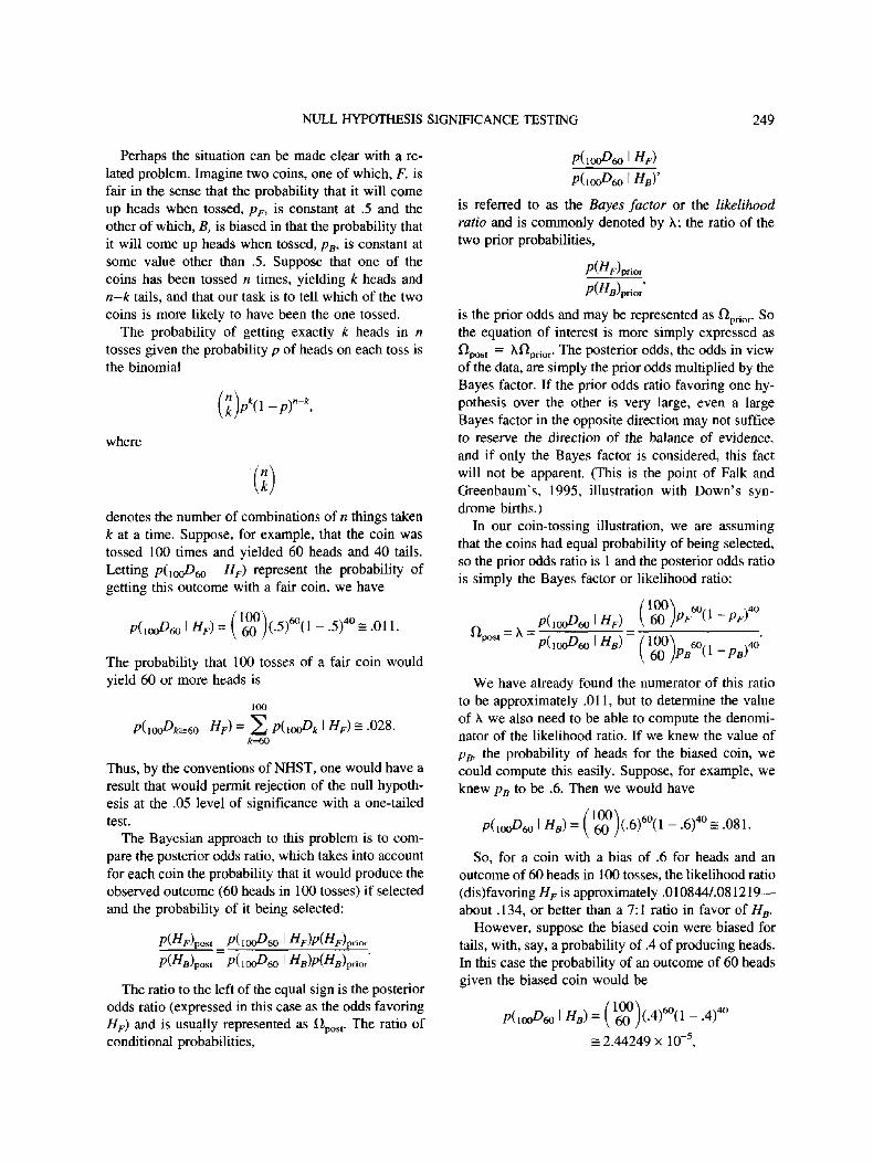
Perhaps the situation can be made clear with a re-
lated problem. Imagine two coins, one of which, F, is
fair in the sense that the probability that it will come
up heads when tossed, pF, is constant at .5 and the
other of which, B, is biased in that the probability that
it will come up heads when tossed, pB, is constant at
some value other than .5. Suppose that one of the
coins has been tossed n times, yielding k heads and
n-k tails, and that our task is to tell which of the two
coins is more likely to have been the one tossed.
The probability of getting exactly k heads in n
tosses given the probability p of heads on each toss is
the binomial
where
denotes the number of combinations of n things taken
k at a time. Suppose, for example, that the coin was
tossed 100 times and yielded 60 heads and 40 tails.
Letting pdooOfjo ! HF) represent the probability of
getting this outcome with a fair coin, we have
The probability that 100 tosses of a fair coin would
yield 60 or more heads is
100
HF) s .028.
Thus, by the conventions of NHST, one would have a
result that would permit rejection of the null hypoth-
esis at the .05 level of significance with a one-tailed
test.
The Bayesian approach to this problem is to com-
pare the posterior odds ratio, which takes into account
for each coin the probability that it would produce the
observed outcome (60 heads in 100 tosses) if selected
and the probability of it being selected:
The ratio to the left of the equal sign is the posterior
odds ratio (expressed in this case as the odds favoring
HF) and is usually represented as Oposl. The ratio of
conditional probabilities,
P( 100^60 I tff)
pdoAo I HB)'
is referred to as the Bayes factor or the likelihood
ratio and is commonly denoted by X; the ratio of the
two prior probabilities,
P(HF\F /prior
P(HB\
is the prior odds and may be represented as nprior. So
the equation of interest is more simply expressed as
flpos, = Xflprior. The posterior odds, the odds in view
of the data, are simply the prior odds multiplied by the
Bayes factor. If the prior odds ratio favoring one hy-
pothesis over the other is very large, even a large
Bayes factor in the opposite direction may not suffice
to reserve the direction of the balance of evidence,
and if only the Bayes factor is considered, this fact
will not be apparent. (This is the point of Falk and
Greenbaum's, 1995, illustration with Down's syn-
drome births.)
In our coin-tossing illustration, we are assuming
that the coins had equal probability of being selected,
so the prior odds ratio is 1 and the posterior odds ratio
is simply the Bayes factor or likelihood ratio:
^ P<.100L>60 ' HB> (1<X)\ 60,. ,40'( 60 )Pa (>--PB>
We have already found the numerator of this ratio
to be approximately .011, but to determine the value
of X we also need to be able to compute the denomi-
nator of the likelihood ratio. If we knew the value of
pB, the probability of heads for the biased coin, we
could compute this easily. Suppose, for example, we
knew pB to be .6. Then we would have
= -081-
So, for a coin with a bias of .6 for heads and an
outcome of 60 heads in 100 tosses, the likelihood ratio
(dis)favoring HF is approximately .010844/.081219 —
about .134, or better than a 7:1 ratio in favor of HB.
However, suppose the biased coin were biased for
tails, with, say, a probability of .4 of producing heads.
In this case the probability of an outcome of 60 heads
given the biased coin would be
= 2.44249 x 10~
250 NICKERSON
Table 2
Likelihood Ratio, X, for Values ofpg Ranging From .05
to.95
PD
.05
.10
.15
.20
.25
.30
.35
.40
.45
.50
.55
.60
.65
.70
.75
.80
.85
.90
.95
(IOCK 60,1 ylO\ 60 №B \ 1 PB)
1.53 x 10~51
2.03 x 1Q-34
1.37X10⁻²⁵
2.11 xlO-1 8
1.37 x 10~14
3.71 x 10-'°
1.99xlO~7
2.44 x 10~5
8.82 x 10⁻⁴
.0108
.0488
.0812
.0474
.0085
.0004
2.32x10-"
8.85 x 1(T1U
2.47 x lO'15
5.76 x 10~26
X
7.08 xlO 4 8
5.34 x 1031
7.89 x 10²²
5.15 x 10¹⁵
7.89x10"
2.92 x 10⁷
5.45 x 10⁴
443.97
12.30
1.00
0.22
0.13
0.23
1.28
29.90
4,681.68
1.23x 10⁷
4.39 x l O 1 2
1.88 x 10²³
Note. \ = p (10(>D«i I #jO/P(i<xAo I HB). F = fair; B = biased.
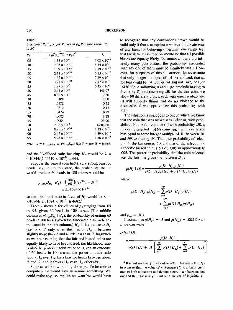
and the likelihood ratio favoring HF would be X =
0.108447(2.44249 x 10~5) = 444.
Suppose the biased coin had a very strong bias for
heads, say, .8. In this case, the probability that it
would produce 60 heads in 100 tosses would be
= 2.3 1624 xlO'6,
so the likelihood ratio in favor of HF would be X =
.010844/(2.31624 x W6) s 4682.4
Table 2 shows X for values of pB ranging from .05
to .95, given 60 heads in 100 tosses. (The middle
column is />(10n£>6o I HB), the probability of getting 60
heads in 100 tosses given the associated bias for heads
indicated in the left column.) HK is favored over HF
(i.e., X < 1) only when the bias on HR is between
slightly more than .5 and a little less than .7. Inasmuch
as we are assuming that the fair and biased coins are
equally likely to have been tossed, the likelihood ratio
is also the posterior odds ratio: so, given an outcome
of 60 heads in 100 tosses, the posterior odds ratio
favors Hfi over HF for a bias for heads between about
.5 and .7, and it favors HF over Hs otherwise.
Suppose we know nothing about pK. To be able to
compute X we would have to assume something. We
could make any assumption we want but would have
to recognize that any conclusions drawn would be
valid only if that assumption were true. In the absence
of any basis for believing otherwise, one might feel
that the default assumption should be that all possible
biases are equally likely. Inasmuch as there are infi-
nitely many possibilities, the probability associated
with any one of them must be infinitely small. How-
ever, for purposes of this illustration, let us assume
that only integer multiples of .01 are allowed; that is,
the bias could be .34, .55, or .74, but not .342, .551, or
.7436. So, disallowing 0 and 1 (to preclude having to
divide by 0) and reserving .50 for the fair coin, we
allow 98 different biases, each with equal probability.
(It will simplify things and do no violence to the
discussion if we approximate this probability with
.01.)
The situation is analogous to one in which we know
that the coin that was tossed was either (a) with prob-
ability .50, the fair coin, or (b) with probability .50, a
randomly selected 1 of 98 coins, each with a different
bias equal to some integer multiple of .01 between .01
and .99, excluding .50. The prior probability of selec-
tion of the fair coin is .50, and that of the selection of
a specific biased coin is .50 x (1/98), or approximately
.005. The posterior probability that the coin selected
was the fair one given the outcome D is
p(HF I D) =p(D \ H,)p(HF)
p(D I HF)p(HF)+p(D I HB)p(HB)"
where
p(D I HB) p(HB) = 2>(D I HB)p(HB)i=\
99
+ ^p(D I HB)p(HB)i=51
andpB = .Oil.
Inasmuch as p(HF) = .5 and p(HB) = .005 for all
i, we can write
p(HF I D)
P(D I HF)
p(D I //,,) + .01
~T
Hs)' J
4 It is not necessary to calculate p(D I Hr) and p(D I HH}
in order to find the value of X. Because (") is a factor com-
mon to both numerator and denominator, it can be cancelledout and the ratio easily found with the use of logarithms.
NULL HYPOTHESIS SIGNIFICANCE TESTING 251
If we apply this equation to the case of 60 heads in
100 losses, we get p(HF I 100 D&,) = .525 and its
complement, p(HB 1 I00 Z)^) = .475, which makes the
posterior odds in favor of HF 1.11.
What the coin-tossing illustration has demonstrated
can be summarized as follows. An outcome—60
heads in 100 tosses—that would be judged by the
conventions of NHST to be significantly different (p
< .05) from what would be produced by a fair coin
would be considered by a Bayesian analysis either
more or less likely to have been produced by the fair
coin than by the biased one, depending on the specif-
ics of the assumed bias. In particular, the Bayesian
analysis showed that the outcome would be judged
more likely to have come from the biased coin only if
the bias for heads were assumed to be greater than .5
and less than .7. If the bias were assumed equally
likely to be anything (to the nearest hundredth) be-
tween .01 and .99 inclusive, the outcome would be
judged to be slightly more likely to have been pro-
duced by the fair coin than by the biased one. These
results do not depend on the prior probability of the
fair coin being smaller than that of the biased one.
Whether it makes sense to assume that all possible
biases are equally likely is a separate question. Un-
doubtedly, alternative assumptions would be more
reasonable in specific instances. In any case, the pos-
terior probability of HF can be computed only if what-
ever is assumed about the bias is made explicit. Other
discussions of the possibility of relatively large p(H0
I D ) in conjunction with relatively small p(D I H0) may
be found in Edwards (1965), Edwards et al. (1963),
I. J. Good (1956, 1981/1983b), and Shafer (1982).
Comment. The belief that p is the probability that
the null hypothesis is true is unquestionably false.
However, as Berger and Sellke (1987) have pointed
out,
like it or not, people do hypothesis testing to obtainevidence as to whether or not the hypotheses are true,and it is hard to fault the vast majority of nonspecialistsfor assuming that, if p — .05, then //„ is very likelywrong. This is especially so since we know of no el-ementary textbooks that teach thatp = .05 is at best veryweak evidence against H0. (p. 114)
Even to many specialists, I suspect, it seems natural
when one obtains a small value of p from a statistical
significance test to conclude that the probability that
the null hypothesis is true must also be very small. If
a small value of p does not provide a basis for this
conclusion, what is the purpose of doing a statistical
significance test? Some would say the answer is that
such tests have no legitimate purpose.
This seems a harsh judgment, especially in view of
the fact that generations of very competent research-
ers have held, and acted on, the belief that a small
value of p is good evidence that the null hypothesis is
false. Of course, the fact that a judgment is harsh does
not make it unjustified, and the fact that a belief has
been held by many people does not make it true.
However, one is led to ask, Is there any justification
for the belief that a small p is evidence that the null is
unlikely to be true? I believe there usually is but that
the justification involves some assumptions that, al-
though usually reasonable, are seldom made explicit.
Suppose one has done an experiment and obtained
a difference between two means that, according to a t
test, is statistically significant at p < .05. If the ex-
perimental procedure and data are consistent with the
assumptions underlying use of the / test, one is now in
a position to conclude that the probability that a
chance process would produce a difference like this is
less than .05, which is to say that if two random
samples were drawn from the same normal distribu-
tion the chance of getting a difference between means
as large as the one obtained is less than 1 in 20. What
one wants to conclude, however, is that the result
obtained probably was not due to chance.
As we have noted, from a Bayesian perspective
assessing the probability of the null hypothesis con-
tingent on the acquisition of some data, p(H0 I />),
requires the updating of the prior probability of the
hypothesis (the probability of the hypothesis before
the acquisition of the data). To do that, one needs the
values of p(D I H0), p(D I //A), p(H0), and p(#A).
However, the only term of the Bayesian equation that
one has in hand, having done NHST, is p(D I //0). If
one is to proceed in the absence of knowledge of the
values of the other terms, one must do so on the basis
of assumptions, and the question becomes what, if
anything, it might be reasonable to assume.
Berger and Sellke (1987) have argued that letting
p(H0) be less than .5 would rarely be justified: "Who,
after all, would be convinced by the statement 'I con-
ducted a Bayesian test of H0, assigning a prior prob-
ability of . 1 to HQ, and my conclusion is that H0 has
posterior probability .05 and should be rejected' " (p.
115). I interpret this argument to mean that even if
one really believes the null hypothesis to be false—as
I assume most researchers do—one should give it at
least equal prior standing with the alternative hypoth-
esis as a matter of conservatism in evidence evalua-
252 NICKERSON
tion. One can also argue that in the absence of com-
pelling reasons for some other assumption, the default
assumption should be that p(H0) equals p(HA) on the
grounds that this is the maximum uncertainty case.
Consider again Equation 1, supposing that/)(f/0) =
p(HA) = .5 and that/)(D I Hn) = .05, so we can write
p(H0 I D) =.05
.05+p(D\HA)'
From this it is clear that with the stated supposition,
p(HQ I D) varies inversely with p(D I HA), the former
going from 1 to approximately .048 as the latter goes
from 0 to 1.
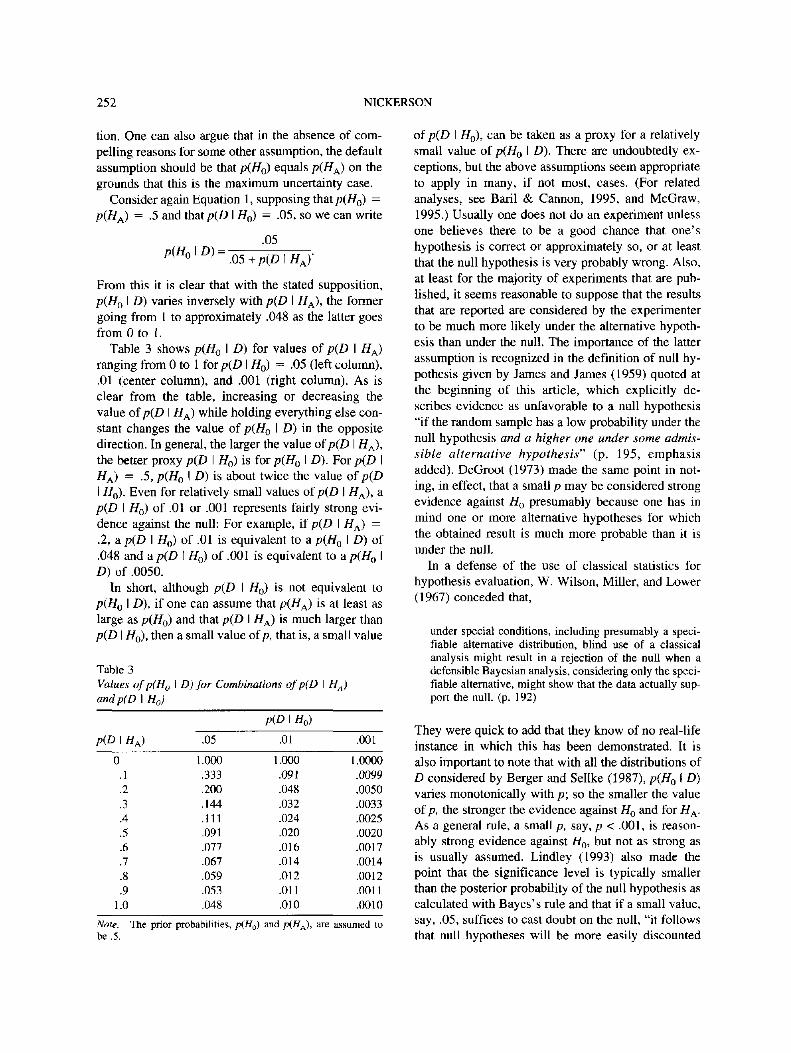
Table 3 shows p(H0 I £>) for values of p(D I #A)
ranging from 0 to 1 for p(D I H0) = .05 (left column),
.01 (center column), and .001 (right column). As is
clear from the table, increasing or decreasing the
value of p(D I HA) while holding everything else con-
stant changes the value of p(H0 I D) in the opposite
direction. In general, the larger the value o(p(D I HA),
the better proxy p(D I H0) is for p(H0 I D). For p(D I
HA) - .5, p(H0 I D) is about twice the value of p(D
I H0). Even for relatively small values of p(D I HA), a
p(D I H0) of .01 or .001 represents fairly strong evi-
dence against the null: For example, if p(D I HA) =
.2, a p(D I H0) of .01 is equivalent to a p(H0 I D) of
.048 and a p(D I H0) of .001 is equivalent to a p(H0 I
D) of .0050.
In short, although p(D I H0) is not equivalent to
p(H0 I D), if one can assume that p(HA) is at least as
large as p(H0) and that p(D I #A) is much larger than
p(D I //0), then a small value of p, that is, a small value
Table 3
Values ofp(H0 I D) for Combinations of p(D I HA)
and pi D I H0j
P(D I H0)
P(D \ HA)
0
.1
.2
.3
.4
.5
.6
.7
.8
.9
1.0
.05
1.000
.333
.200
.144
.111
.091
.077
.067
.059
.053
.048
.01
1.000
.091
.048
.032
.024
.020
.016
.014
.012
.011
.010
.001
1.0000
.0099
.0050
.0033
.0025
.0020
.0017
.0014
.0012
.0011
.0010
Note, The prior probabilities, p(Ha) and p(HA), are assumed to
be .5.
of p(D I //0), can be taken as a proxy for a relatively
small value of p(H0 I D). There are undoubtedly ex-
ceptions, but the above assumptions seem appropriate
to apply in many, if not most, cases. (For related
analyses, see Baril & Cannon, 1995, and McGraw,
1995.) Usually one does not do an experiment unless
one believes there to be a good chance that one's
hypothesis is correct or approximately so, or at least
that the null hypothesis is very probably wrong. Also,
at least for the majority of experiments that are pub-
lished, it seems reasonable to suppose that the results
that are reported are considered by the experimenter
to be much more likely under the alternative hypoth-
esis than under the null. The importance of the latter
assumption is recognized in the definition of null hy-
pothesis given by James and James (1959) quoted at
the beginning of this article, which explicitly de-
scribes evidence as unfavorable to a null hypothesis
"if the random sample has a low probability under the
null hypothesis and a higher one under some admis-
sible alternative hypothesis" (p. 195, emphasis
added). DeGroot (1973) made the same point in not-
ing, in effect, that a small p may be considered strong
evidence against H0 presumably because one has in
mind one or more alternative hypotheses for which
the obtained result is much more probable than it is
under the null.
In a defense of the use of classical statistics for
hypothesis evaluation, W. Wilson, Miller, and Lower
(1967) conceded that,
under special conditions, including presumably a speci-fiable alternative distribution, blind use of a classicalanalysis might result in a rejection of the null when adefensible Bayesian analysis, considering only the speci-fiable alternative, might show that the data actually sup-port the null. (p. 192)
They were quick to add that they know of no real-life
instance in which this has been demonstrated. It is
also important to note that with all the distributions of
D considered by Berger and Sellke (1987), p(H0 I D)
varies monotonically with p; so the smaller the value
of p, the stronger the evidence against H0 and for HA.
As a general rule, a small p, say, p < .001, is reason-
ably strong evidence against H0, but not as strong as
is usually assumed. Lindley (1993) also made the
point that the significance level is typically smaller
than the posterior probability of the null hypothesis as
calculated with Bayes' s rule and that if a small value,
say, .05, suffices to cast doubt on the null, "it follows
that null hypotheses will be more easily discounted
NULL HYPOTHESIS SIGNIFICANCE TESTING 253
using Fisher's method rather than the Bayesian ap-
proach" (p. 25). (This puts Melton's, 1962, well-
publicized refusal to publish results with/j < .05 while
editor of the Journal of Experimental Psychology in a
somewhat more favorable light than do some of the
comments of his many critics.)
The numbers in Table 3 represent the condition in
which p(HQ) = p(HA) = .5. We should note that
when everything else is held constant, p(H01 D) varies
directly with p(H0) and of course inversely with
p(HA). We can also look at the situation in terms of
the Bayes factor or likelihood ratio (I. J. Good, 19817
1983b) and ask not what the probability is of either
HA or H0 in view of the data, but which of the two
hypotheses the data favor. This approach does not
require any knowledge or assumptions about p(HA) or
p(H0), but it does require knowledge, or an estimate,
of the probability of the obtained result, conditional
on the alternative hypothesis, p(D I #A). Whenever
the probability of a result conditional on the alterna-tive hypothesis is greater than the probability of the
result conditional on the null, X > 1, the alternative
hypothesis gains support. The strength of the support
is indicated by the size of X. (I. J. Good, 1981/1983b,
pointed out that the logarithm of this ratio was called
the weight of evidence in favor of //A by C. S. Peirce,
1878/1956, as well as by himself [I. J. Good, 1950]
and others more recently.)The fact that evaluating hypotheses in terms of the
Bayes factor alone does not require specification of
the prior probabilities of the hypotheses is an advan-
tage. However, it is also a limitation of the approach
inasmuch as it gives one only an indication of the
direction and degree of change in the evidence favor-
ing one hypothesis over the other but does not provide
an indication of what the relative strengths of the
competing hypotheses—in view of the results—are.
In my view, the most important assumption re-quired by the belief that p can be a reasonable proxy
for p(H0 I D) is that p(D I HA) is much greater than
p(D I H0). It seems likely that, if asked, most experi-
menters would say that they make this assumption.
But is it a reasonable one? I find it easier to imaginesituations in which it is than situations in which it is
not. On the other hand, it is not hard to think of cases
in which the probability of a given result would be
very small under either the null or the alternative hy-pothesis. One overlooks this possibility when one ar-gues that because the prior probability of a specified
event was small, the event, having occurred, musthave had a nonchance cause.
Essentially all events, if considered in detail, are
low-probability events, and for this reason the fact
that a low-probability event has occurred is not good
evidence that it was not a chance event. (Imagine that
10 tosses of a coin yielded a tails [T] and heads [H]
sequence of TTHTHHHTHT. The probably of getting
precisely this sequence given a fair coin, p(D I
chance), in 10 consecutive tosses is very small, less
than .001. However, it clearly does not follow that the
sequence must have been produced by a nonchance
process.) I. J. Good (1981/1983b) applied this fact tothe problem of hypothesis evaluation this way:
We never reject a hypothesis H merely because an event£ of very small probability (given H) has occurred al-though we often carelessly talk as if that were our reasonfor rejection. If the result £ of an experiment or obser-vation is described in sufficient detail its probabilitygiven H is nearly always less than say one in a million,
(p. 133)
I. J. Good (1981/1983b) quoted Jeffreys (1961) on the
same point: "If mere probability of the observation,given the hypothesis, was the criterion, any hypoth-
esis whatever would be rejected" (p. 315). What oneneeds to know is how the probability of the event in
question given the null hypothesis compares with theprobability of the event given the alternative hypoth-
esis.
Usually p(D I HA) is not known—often the exact
nature of f/A is not specified—and sometimes one
may have little basis for even making an assumption
about it. If one can make an assumption about the
value of p(D I HA), one may have the basis for an
inference from p to p(H0 I D), or at least from p to X,
that will be valid under that assumption. It is desir-
able, of course, when inferences that rest on assump-tions are made that those assumptions be clearly iden-
tified. It must be noted, too, that, in the absence of
knowledge, or some assumption, about the value of
p(D I HA), p does not constitute a reliable basis formaking an inference about either p(H0 I D) or X. We
can say, however, that in general with other thingsbeing equal, the smaller the value of p, the larger the
Bayes factor favoring #A. The claim that p is likelyto be smaller than p(H0 I D) is not necessarily an
argument against using NHST in principle but only abasis for concluding that a small p is not as strongevidence against the null hypothesis as its value sug-
gests, and it is obviously a basis for not equating p
with p(H0 I D).
254 NICKERSON
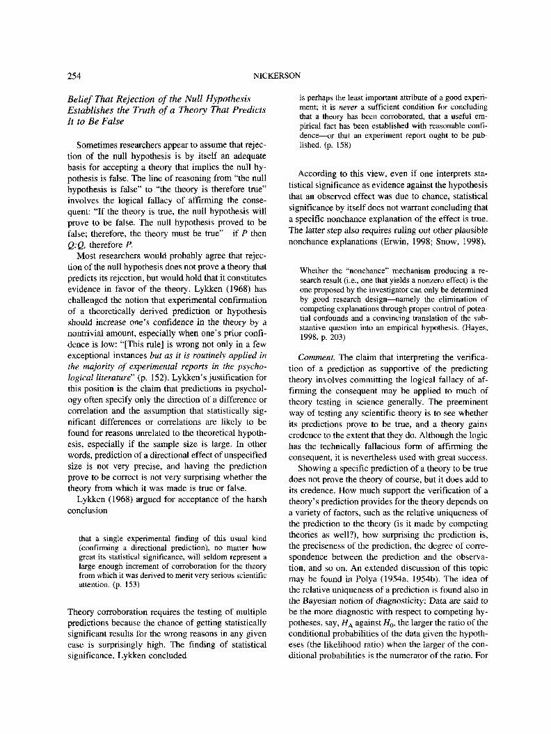
Belief That Rejection of the Null HypothesisEstablishes the Truth of a Theory That PredictsIt to Be False
Sometimes researchers appear to assume that rejec-
tion of the null hypothesis is by itself an adequate
basis for accepting a theory that implies the null hy-
pothesis is false. The line of reasoning from "the null
hypothesis is false" to "the theory is therefore true"
involves the logical fallacy of affirming the conse-
quent: "If the theory is true, the null hypothesis will
prove to be false. The null hypothesis proved to be
false; therefore, the theory must be true"—if P then
Q:Q, therefore P.
Most researchers would probably agree that rejec-
tion of the null hypothesis does not prove a theory that
predicts its rejection, but would hold that it constitutes
evidence in favor of the theory. Lykken (1968) has
challenged the notion that experimental confirmation
of a theoretically derived prediction or hypothesis
should increase one's confidence in the theory by a
nontrivial amount, especially when one's prior confi-
dence is low: "[This rule] is wrong not only in a few
exceptional instances but as it is routinely applied in
the majority of experimental reports in the psycho-
logical literature" (p. 152). Lykken's justification for
this position is the claim that predictions in psychol-
ogy often specify only the direction of a difference or
correlation and the assumption that statistically sig-
nificant differences or correlations are likely to be
found for reasons unrelated to the theoretical hypoth-
esis, especially if the sample size is large. In other
words, prediction of a directional effect of unspecified
size is not very precise, and having the prediction
prove to be correct is not very surprising whether the
theory from which it was made is true or false.
Lykken (1968) argued for acceptance of the harsh
conclusion
that a single experimental finding of this usual kind(confirming a directional prediction), no matter howgreat its statistical significance, will seldom represent alarge enough increment of corroboration for the theoryfrom which it was derived to merit very serious scientificattention, (p. 153)
Theory corroboration requires the testing of multiple
predictions because the chance of getting statistically
significant results for the wrong reasons in any given
case is surprisingly high. The finding of statistical
significance, Lykken concluded
is perhaps the least important attribute of a good experi-ment; it is never a sufficient condition for concludingthat a theory has been corroborated, that a useful em-pirical fact has been established with reasonable confi-dence—or that an experiment report ought to be pub-lished, (p. 158)
According to this view, even if one interprets sta-
tistical significance as evidence against the hypothesis
that an observed effect was due to chance, statistical
significance by itself does not warrant concluding that
a specific nonchance explanation of the effect is true.
The latter step also requires ruling out other plausible
nonchance explanations (Erwin, 1998; Snow, 1998).
Whether the "nonchance" mechanism producing a re-search result (i.e., one that yields a nonzero effecl) is theone proposed by the investigator can only be determinedby good research design—namely the elimination ofcompeting explanations through proper control of poten-tial confounds and a convincing translation of the sub-stantive question into an empirical hypothesis. (Hayes,1998, p. 203)
Comment. The claim that interpreting the verifica-
tion of a prediction as supportive of the predicting
theory involves committing the logical fallacy of af-
firming the consequent may be applied to much of
theory testing in science generally. The preeminent
way of testing any scientific theory is to see whether
its predictions prove to be true, and a theory gains
credence to the extent that they do. Although the logic
has the technically fallacious form of affirming the
consequent, it is nevertheless used with great success.
Showing a specific prediction of a theory to be true
does not prove the theory of course, but it does add to
its credence. How much support the verification of a
theory's prediction provides for the theory depends on
a variety of factors, such as the relative uniqueness of
the prediction to the theory (is it made by competing
theories as well?), how surprising the prediction is,
the preciseness of the prediction, the degree of corre-
spondence between the prediction and the observa-
tion, and so on. An extended discussion of this topic
may be found in Polya (1954a, 1954b). The idea of
the relative uniqueness of a prediction is found also in
the Bayesian notion of diagnosticity: Data are said to
be the more diagnostic with respect to competing hy-
potheses, say, HA against H0, the larger the ratio of the
conditional probabilities of the data given the hypoth-
eses (the likelihood ratio) when the larger of the con-
ditional probabilities is the numerator of the ratio. For
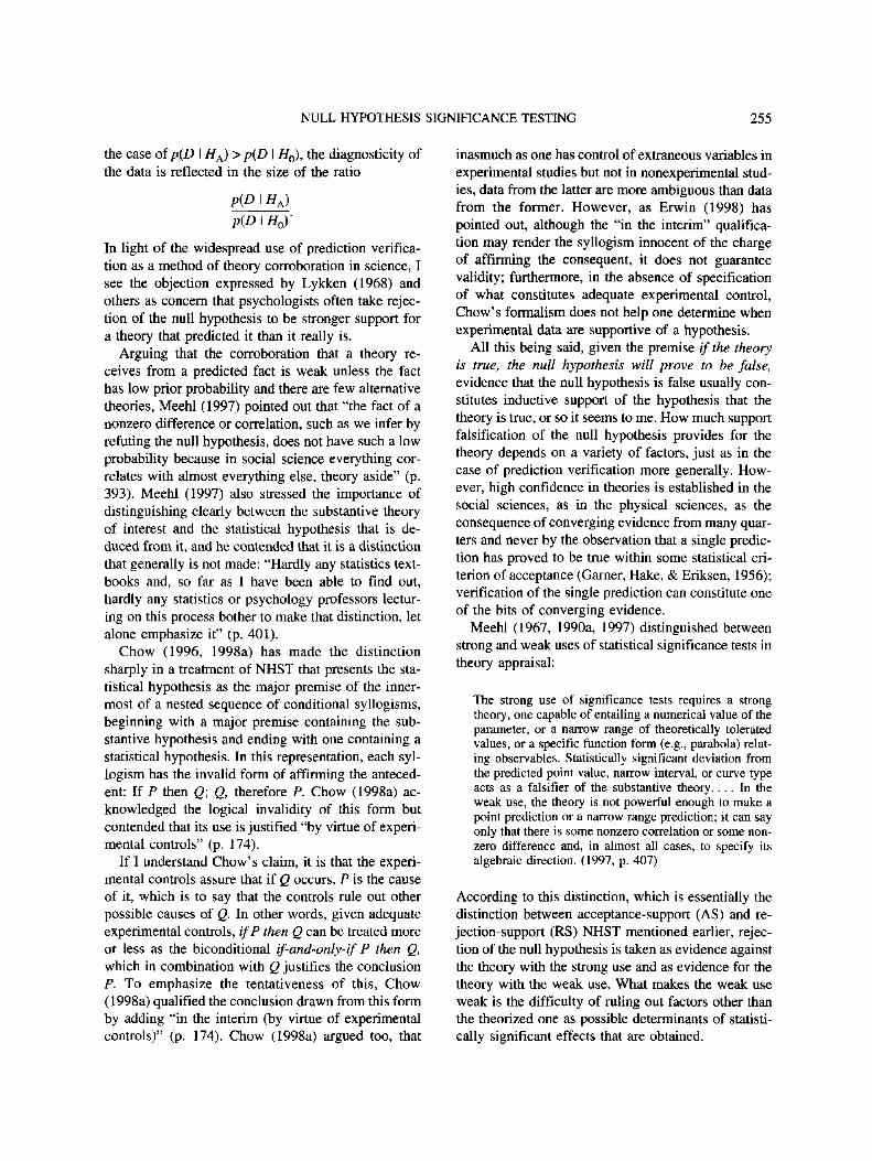
NULL HYPOTHESIS SIGNIFICANCE TESTING 255
the case of p(D I H A ) > p(D I #„), the diagnosticity of
the data is reflected in the size of the ratio
P(D I HA)
p(D I H0Y
In light of the widespread use of prediction verifica-
tion as a method of theory corroboration in science, I
see the objection expressed by Lykken (1968) and
others as concern that psychologists often take rejec-
tion of the null hypothesis to be stronger support for
a theory that predicted it than it really is.
Arguing that the corroboration that a theory re-
ceives from a predicted fact is weak unless the fact
has low prior probability and there are few alternative
theories, Meehl (1997) pointed out that "the fact of a
nonzero difference or correlation, such as we infer by
refuting the null hypothesis, does not have such a low
probability because in social science everything cor-
relates with almost everything else, theory aside" (p.
393). Meehl (1997) also stressed the importance of
distinguishing clearly between the substantive theory
of interest and the statistical hypothesis that is de-
duced from it, and he contended that it is a distinction
that generally is not made: "Hardly any statistics text-
books and, so far as I have been able to find out,
hardly any statistics or psychology professors lectur-
ing on this process bother to make that distinction, let
alone emphasize it" (p. 401).
Chow (1996, 1998a) has made the distinction
sharply in a treatment of NHST that presents the sta-
tistical hypothesis as the major premise of the inner-
most of a nested sequence of conditional syllogisms,
beginning with a major premise containing the sub-
stantive hypothesis and ending with one containing a
statistical hypothesis. In this representation, each syl-
logism has the invalid form of affirming the anteced-
ent: If P then Q; Q, therefore P. Chow (1998a) ac-
knowledged the logical invalidity of this form but
contended that its use is justified "by virtue of experi-
mental controls" (p. 174).
If I understand Chow's claim, it is that the experi-
mental controls assure that if Q occurs, P is the cause
of it, which is to say that the controls rule out other
possible causes of Q. In other words, given adequate
experimental controls, ifP then Q can be treated more
or less as the biconditional if-and-only-if P then Q,
which in combination with Q justifies the conclusion
P. To emphasize the tentativeness of this, Chow
(1998a) qualified the conclusion drawn from this form
by adding "in the interim (by virtue of experimental
controls)" (p. 174). Chow (1998a) argued too, that
inasmuch as one has control of extraneous variables in
experimental studies but not in nonexperimental stud-
ies, data from the latter are more ambiguous than data
from the former. However, as Erwin (1998) has
pointed out, although the "in the interim" qualifica-
tion may render the syllogism innocent of the charge
of affirming the consequent, it does not guarantee
validity; furthermore, in the absence of specification
of what constitutes adequate experimental control,
Chow's formalism does not help one determine when
experimental data are supportive of a hypothesis.
All this being said, given the premise if the theory
is true, the null hypothesis will prove to be false,
evidence that the null hypothesis is false usually con-
stitutes inductive support of the hypothesis that the
theory is true, or so it seems to me. How much support
falsification of the null hypothesis provides for the
theory depends on a variety of factors, just as in the
case of prediction verification more generally. How-
ever, high confidence in theories is established in the
social sciences, as in the physical sciences, as the
consequence of converging evidence from many quar-
ters and never by the observation that a single predic-
tion has proved to be true within some statistical cri-
terion of acceptance (Garner, Hake, & Eriksen, 1956);
verification of the single prediction can constitute one
of the bits of converging evidence.
Meehl (1967, 1990a, 1997) distinguished between
strong and weak uses of statistical significance tests in
theory appraisal:
The strong use of significance tests requires a strongtheory, one capable of entailing a numerical value of theparameter, or a narrow range of theoretically toleratedvalues, or a specific function form (e.g., parabola) relat-ing observables. Statistically significant deviation fromthe predicted point value, narrow interval, or curve typeacts as a falsifier of the substantive theory.... In theweak use, the theory is not powerful enough to make apoint prediction or a narrow range prediction; it can sayonly that there is some nonzero correlation or some non-zero difference and, in almost all cases, to specify itsalgebraic direction. (1997, p. 407)
According to this distinction, which is essentially the
distinction between acceptance-support (AS) and re-
jection-support (RS) NHST mentioned earlier, rejec-
tion of the null hypothesis is taken as evidence against
the theory with the strong use and as evidence for the
theory with the weak use. What makes the weak use
weak is the difficulty of ruling out factors other than
the theorized one as possible determinants of statisti-
cally significant effects that are obtained.
256 NICKERSON
Meehl (1997) cautioned that both the strong and
weak uses are subject to misinterpretation or abuse.
The strong use risks rejection of a theory when in fact
a significant difference from a prediction could have
been due to any of a variety of reasons other than that
the theory was incorrect. The weak use is abused
when rejection of the null hypothesis is interpreted as
powerful support for a weak theory. Moreover, al-
though most researchers would undoubtedly agree
that strong theories are much to be preferred over
weak ones, Meehl (1997) expressed some reserva-
tions about the strong use of NHST:
Even when the theory is so strong as to permit point
predictions . . . the uncertainty of the auxiliaries, the
doubtfulness of the ceteris paribus clause, the unreliabil-
ity of measuring instruments, and so on, leave us won-
dering just what we should say when what appears to bea strong Popperian test is successfully passed or—even
more so—is failed, (p. 411).
Meehl (1997) noted the possibility that, especially in
the early stages of theory construction, an outcome
that could be taken literally as a falsification of the
theory could equally well be seen as an encouraging
sign:
The history of science shows that—even for the mostpowerful of the exact sciences—numerical closeness to a
theoretically predicted observational value is commonly
taken as corroborative of a strong theory even if, strictly
speaking, it is a falsifier because the observed value
deviates "significantly" from the value predicted, (p.
411)
It seems there is no escaping the use of judgment in
the use and interpretation of statistical significance
tests.
Belief That a Small p Is Evidence That theResults Are Replicable
Often statistical significance is taken as evidence of
the replicability (or reliability) of the obtained experi-
mental outcome; a small value of p is considered to
mean a strong likelihood of getting the same results
on another try (Coleman, 1964; Evans, 1985; R. J.
Harris, 1997a; Levy, 1967; Melton, 1962; Reaves,
1992; Shaughnessy & Zechmeister, 1994). In some
cases, the complement of p appears to be interpreted
as an indication of the exact probability of replication.
Nunnally (1975), for example, has said that statistical
significance at the .05 level can be taken to mean that
the odds are 95 out of 100 that the observed difference
will hold up in future investigations. A survey of aca-
demic psychologists by Oakes (1986) revealed that
60% of the participants held essentially this belief.
Carver (1978) referred to this belief as the "repli-
cability or reliability fantasy," inasmuch as "nothing
in the logic of statistics allows a statistically signifi-
cant result to be interpreted as directly reflecting the
probability that the result can be replicated" (p. 386).
Several other writers have noted that a small p value
does not guarantee replicability of experimental re-
sults (Bakan, 1966; Falk, 1998b; Falk & Greenbaum,
1995; Gigerenzer, 1993; Lykken, 1968; Rosenthal,
1991; Sohn, 1998b; Thompson, 1996), but the belief
that it does appears to be very common among psy-
chologists. (Sohn, 1998b, pointed out that even the
fact that a hypothesis is true does not guarantee the
replication of an experimental finding.)
Comment. It is important to distinguish different
connotations that replication can have in this context.
It can mean getting exactly, or almost exactly, the
same effect—direction and size—in a repetition of an
experiment in which conditions are as nearly the same
as those of the original as they can be made, or it can
mean getting a result that will support the same con-
clusion (reject or nonreject) regarding the null hypoth-
esis. Finer distinctions can be made within the latter
category (Lykken, 1968; Sidman, 1960). A small p
does not guarantee replicability in either of the two
senses mentioned. Definitely, p does not represent the
complement of the probability that a result will rep-
licate in either of these senses.
An argument can be (and has been) made, however,
that a small p does constitute a reasonable basis for
expectation with respect to the latter sense—that hav-
ing obtained a statistically significant result, the
smaller the value of p, the more likely it is that a
replication of the experiment would again produce a
statistically significant result (Greenwald et al., 1996;
Rosnow & Rosenthal, 1989b; Scarr, 1997). Other
things equal, in this sense a bet on replicability of a
result that yielded p < .001 would be safer than a bet
on the replicability of a result that yielded p < .05; p
< .001 tells one that the result obtained would be
expected less than 1 time in a thousand when the null
hypothesis is true, whereas p < .05 tells one the result
would be expected less than 1 time in 20 when the
null is true. The evidence that the result is real (non-
chance) is stronger in the former case and thus pro-
vides a firmer basis for the expectation of replication
(in the sense of another statistically significant result).
Schmidt and Hunter (1997) contended that "repro-
ducibility requires high statistical power. Even if all
NULL HYPOTHESIS SIGNIFICANCE TESTING 257
other aspects of a study are carried out in a scientifi-
cally impeccable manner, the finding of statistical sig-
nificance in the original study will not replicate con-
sistently if statistical power is low" (p. 44). It needs to
be noted, however, that this observation pertains spe-
cifically to the statistical power of the experiment that
constitutes the replication attempt. It can be argued
that the smaller the sample and the smaller the a of
the original experiment, the larger the effect size must
have been to yield a significant result, and that the
larger the effect size, the more likely it should yield
significance on subsequent experimentation. Inas-
much as the effect size in the population does not
change as a consequence of experimental procedure,
the probability of getting a significant result in a rep-
lication study can be increased by increasing the
power of that study relative to that of the original by
increasing the sample size.
Discussions of replicability usually do not consider
the replicability of nonsignificant results. However, it
should be noted that if the results of an experiment
yield a large p, it seems likely that a repetition of the
experiment would again yield a nonsignificant value
of p. So, if obtaining nonsignificant results a second
time is considered a replication, a case might be made
for the claim that a large p suggests the likelihood of
replicability, but in this case of a nonsignificant result.
Whether nonsignificance tends to replicate more con-
sistently than significance is an empirical question;
Schmidt and Hunter (1997) have suggested that it
does not.
.06. This is not unusual, in my experience. Undoubt-
edly, such language often gets modified as a conse-
quence of the editorial review process, but certainly
not all of it does; and the fact that it appears in un-
edited manuscripts indicates the need for greater
awareness of the problem.
Comment. The value ofp is not a reliable indication
of the magnitude of an effect (Bracey, 1991; Cohen,
1994; Rosenthal, 1993); as Sohn (1998b) has said,
"There is no guarantee, from SS [statistical signifi-
cance], that the mean difference is greater than infini-
tesimal" (p. 299). On the other hand, p and effect size
are not completely independent, and belief that one
can be an indication of the other has some foundation.
For fixed sample size and variability, the larger an
effect, the smaller that p is likely to be, and vice versa.
The proviso is important, however, because with a
large sample or small variability, even a very small
effect can prove to be statistically significant (yield a
small p), and with a small sample or large variability
even a large effect can fail to attain a conventional
level of significance. Parenthetically, we should also
note that a large effect is not a guarantee of impor-
tance, any more than a small p value is; although, as
a general rule, a large effect seems more likely to be
important than a small one, at least from a practical
point of view.
Belief That Statistical Significance MeansTheoretical or Practical Significance
Belief That a Small Value of p Means aTreatment Effect of Large Magnitude
It is difficult to know how common this belief is.
My guess is that, if asked, most researchers would
judge it to be false, but this is just a guess. In reporting
results of experiments, however, researchers often use
language that lends itself to this type of misinterpre-
tation. Reference to effects as "significant" rather than
as "statistically significant" invites such misinterpre-
tation, unless the context makes it clear that the latter
connotation is intended; and often the context does
not rule out the less restrictive meaning.
Other ways of qual i fy ing "significant"—
"extremely," "barely," "marginally"—can also con-
vey inappropriate meanings. For example, I recently
reviewed a manuscript that described a response time
that was about 16% slower than another as being
"marginally slower" than the latter, because .05 < p <
Confusion between statistical and theoretical or
practical significance (or what is sometimes called
substantive significance, or in clinical contexts, clini-
cal significance) appears to be a continuing problem,
despite warnings against it by many writers over
many years (Berkson, 1938, 1942; Cohen, 1965,
1994; Grant, 1962; Guttman, 1977; Hays, 1994; Ja-
cobson, Follette, & Revenstorf, 1984; Rosenthal,
1993; Shaver, 1985, 1993; Tyler, 1931). When one
concludes on the basis of a statistical test that the
difference between two means is statistically signifi-
cant, one is saying only that a difference of the ob-
served magnitude is unlikely to be obtained between
two samples drawn at random from the same popula-
tion. Even assuming that one has a basis for going
beyond this and concluding that the difference is
real—caused by something other than chance—it
does not follow that it is either interesting or impor-
tant. Rosenthal (1983) has argued that because of the
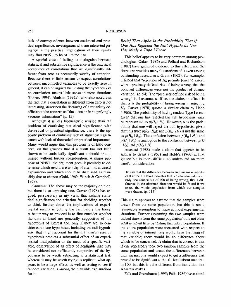
258 NICKERSON
lack of correspondence between statistical and prac-
tical significance, investigators who are interested pri-
marily in the practical implications of their results
may find NHST to be of limited use.
A special case of failing to distinguish between
statistical and substantive significance is the uncritical
acceptance of correlations that are significantly dif-
ferent from zero as necessarily worthy of attention.
Because there is little reason to expect correlations
between uncontrolled variables to be exactly zero in
general, it can be argued that testing the hypothesis of
no correlation makes little sense in most situations
(Cohen, 1994). Abelson (1997a), who also noted that
the fact that a correlation is different from zero is not
interesting, described the declaring of a reliability co-
efficient to be nonzero as "the ultimate in stupefyingly
vacuous information" (p. 13).
Although it is less frequently discussed than the
problem of confusing statistical significance with
theoretical or practical significance, there is the op-
posite problem of confusing lack of statistical signifi-
cance with lack of theoretical or practical importance.
Many would argue that this problem is of little con-
cern, on the grounds that if a result has not been
shown to be statistically significant it should be dis-
missed without further consideration. A major pur-
pose of NHST, the argument goes, it precisely to de-
termine which results are worthy of attempts at causal
explanation and which should be dismissed as plau-
sibly due to chance (Gold, 1969; Winch & Campbell,
1969).
Comment. The above may be the majority opinion,
but there is an opposing one. Carver (1978) has ar-
gued, persuasively in my view, that making statis-
tical significance the criterion for deciding whether
to think further about the implications of experi-
mental results is putting the cart before the horse.
A better way to proceed is to first consider whether
the data in hand are generally supportive of the
hypothesis of interest and, only if they are, to con-
sider candidate hypotheses, including the null hypoth-
esis, that might account for them. If one's research
hypothesis predicts a substantial effect of an experi-
mental manipulation on the mean of a specific vari-
able, observation of an effect of negligible size may
be considered not sufficiently supportive of the hy-
pothesis to be worth subjecting to a statistical test;
whereas it may be worth trying to replicate what ap-
pears to be a large effect, as well as testing to see if
random variation is among the plausible explanations
for it.
Belief That Alpha Is the Probability That ifOne Has Rejected the Null Hypothesis OneHas Made a Type I Error
This belief appears to be very common among psy-
chologists. Oakes (1986) and Pollard and Richardson
(1987) have gathered evidence to this effect, and the
literature provides many illustrations of it even among
outstanding researchers. Grant (1962), for example,
claimed that "rejection of Ha permits [one] to assert,
with a precisely defined risk of being wrong, that the
obtained differences were not the product of chance
variation" (p. 54). The "precisely defined risk of being
wrong" is, I assume, ct. If so, the claim, in effect, is
that a is the probability of being wrong in rejecting
H0. Carver (1978) quoted a similar claim by Hebb
(1966). The probability of having made a Type I error,
given that one has rejected the null hypothesis, may
be represented as p(H0 I /?„). However, a is the prob-
ability that one will reject the null hypothesis, given
that it is true: p(R0 I H0); andp(/?0 I H Q ) is not the same
as p(H0 I R0). The confusion between p(R0 I H0) and
p(H0 I R0) is analogous to the confusion between p(D
I H0) and p(H0 I D).
Anastasi (1988) made a claim that appears to be
similar to Grant's (1962) and Hebb's (1966) at first
glance but is more difficult to understand on more
careful consideration:
To say that the difference between two means is signifi-
cant at the .01 level indicates that we can conclude, with
only one chance out of 100 of being wrong, that a dif-
ference in the obtained direction would be found if wetested the whole population from which our samples
were drawn, (p. 115)
This claim appears to assume that the samples were
drawn from the same population, but this is not a
reasonable assumption to make in most experimental
situations. Further (assuming the two samples were
indeed drawn from the same population) it is not clear
what is meant here by testing that entire population. If
the entire population were measured with respect to
the variable of interest, one would have the mean of
that variable; there would be no difference about
which to be concerned. A claim that is correct is that
if one repeatedly took two random samples from the
same population and tested the differences between
their means, one would expect to get a difference that
proved to be significant at the .01 level about one time
in 100, but this is quite different from that claim that
Anastasi makes.
Falk and Greenbaum (1995; Falk, 1986) have noted
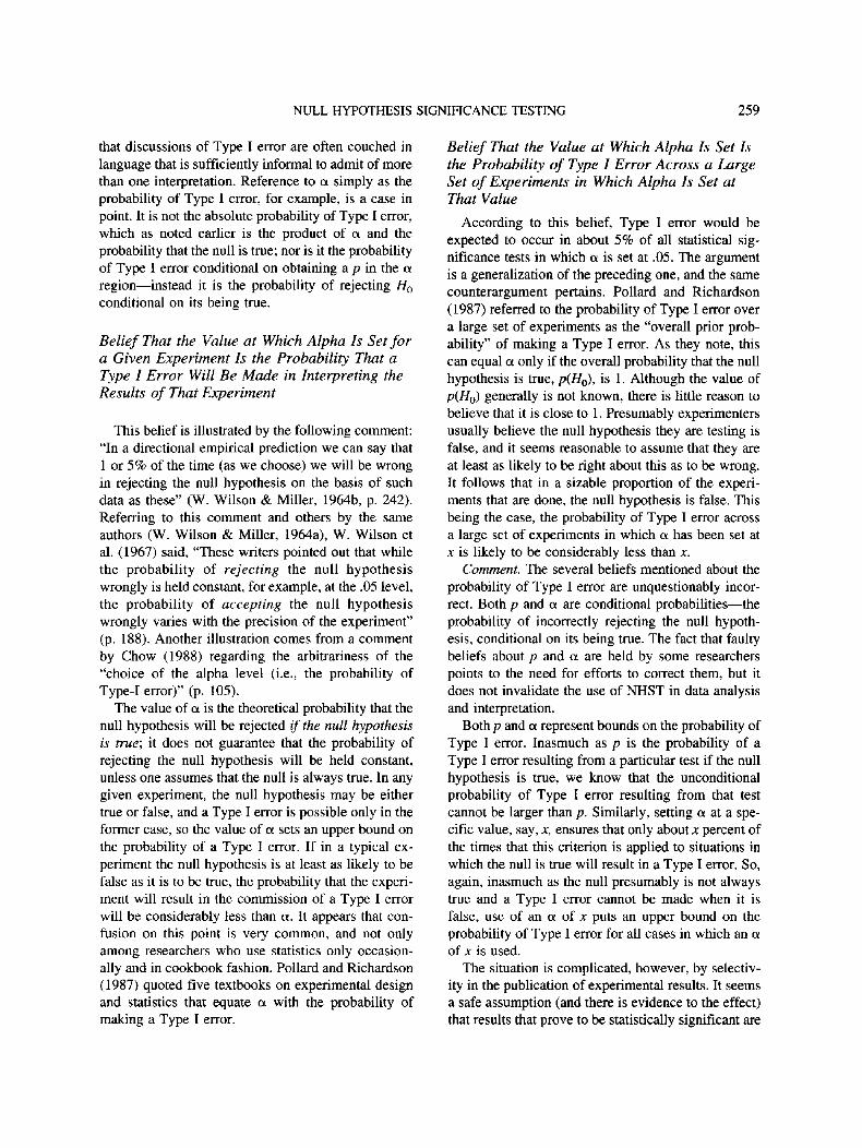
NULL HYPOTHESIS SIGNIFICANCE TESTING 259
that discussions of Type I error are often couched in
language that is sufficiently informal to admit of more
than one interpretation. Reference to a simply as the
probability of Type I error, for example, is a case in
point. It is not the absolute probability of Type I error,
which as noted earlier is the product of a and the
probability that the null is true; nor is it the probability
of Type I error conditional on obtaining a p in the a
region—instead it is the probability of rejecting H0
conditional on its being true.
Belief That the Value at Which Alpha Is Set fora Given Experiment Is the Probability That aType I Error Will Be Made in Interpreting theResults of That Experiment
This belief is illustrated by the following comment:
"In a directional empirical prediction we can say that
1 or 5% of the time (as we choose) we will be wrong
in rejecting the null hypothesis on the basis of such
data as these" (W. Wilson & Miller, 1964b, p. 242).
Referring to this comment and others by the same
authors (W. Wilson & Miller, 1964a), W. Wilson et
al. (1967) said, "These writers pointed out that while
the probability of rejecting the null hypothesis
wrongly is held constant, for example, at the .05 level,
the probability of accepting the null hypothesis
wrongly varies with the precision of the experiment"
(p. 188). Another illustration comes from a comment
by Chow (1988) regarding the arbitrariness of the
"choice of the alpha level (i.e., the probability of
Type-I error)" (p. 105).
The value of a is the theoretical probability that the
null hypothesis will be rejected if the null hypothesis
is true; it does not guarantee that the probability of
rejecting the null hypothesis will be held constant,
unless one assumes that the null is always true. In any
given experiment, the null hypothesis may be either
true or false, and a Type I error is possible only in the
former case, so the value of cc sets an upper bound on
the probability of a Type I error. If in a typical ex-
periment the null hypothesis is at least as likely to be
false as it is to be true, the probability that the experi-
ment will result in the commission of a Type I error
will be considerably less than a. It appears that con-
fusion on this point is very common, and not only
among researchers who use statistics only occasion-
ally and in cookbook fashion. Pollard and Richardson
(1987) quoted five textbooks on experimental design
and statistics that equate a with the probability of
making a Type I error.
Belief That the Value at Which Alpha Is Set Isthe Probability of Type I Error Across a LargeSet of Experiments in Which Alpha Is Set atThat Value
According to this belief, Type I error would be
expected to occur in about 5% of all statistical sig-
nificance tests in which a is set at .05. The argument
is a generalization of the preceding one, and the same
counterargument pertains. Pollard and Richardson
(1987) referred to the probability of Type I error over
a large set of experiments as the "overall prior prob-
ability" of making a Type I error. As they note, this
can equal a only if the overall probability that the null
hypothesis is true, p(H0), is 1. Although the value of
p(Hu) generally is not known, there is little reason to
believe that it is close to 1. Presumably experimenters
usually believe the null hypothesis they are testing is
false, and it seems reasonable to assume that they are
at least as likely to be right about this as to be wrong.
It follows that in a sizable proportion of the experi-
ments that are done, the null hypothesis is false. This
being the case, the probability of Type I error across
a large set of experiments in which a has been set at
x is likely to be considerably less than jc.
Comment. The several beliefs mentioned about the
probability of Type I error are unquestionably incor-
rect. Both p and a are conditional probabilities—the
probability of incorrectly rejecting the null hypoth-
esis, conditional on its being true. The fact that faulty
beliefs about p and a are held by some researchers
points to the need for efforts to correct them, but it
does not invalidate the use of NHST in data analysis
and interpretation.
Bothp and a represent bounds on the probability of
Type I error. Inasmuch as p is the probability of a
Type I error resulting from a particular test if the null
hypothesis is true, we know that the unconditional
probability of Type I error resulting from that test
cannot be larger than p. Similarly, setting a at a spe-
cific value, say, x, ensures that only about x percent of
the times that this criterion is applied to situations in
which the null is true will result in a Type I error. So,
again, inasmuch as the null presumably is not always
true and a Type I error cannot be made when it is
false, use of an a of x puts an upper bound on the
probability of Type I error for all cases in which an a
of x is used.
The situation is complicated, however, by selectiv-
ity in the publication of experimental results. It seems
a safe assumption (and there is evidence to the effect)
that results that prove to be statistically significant are
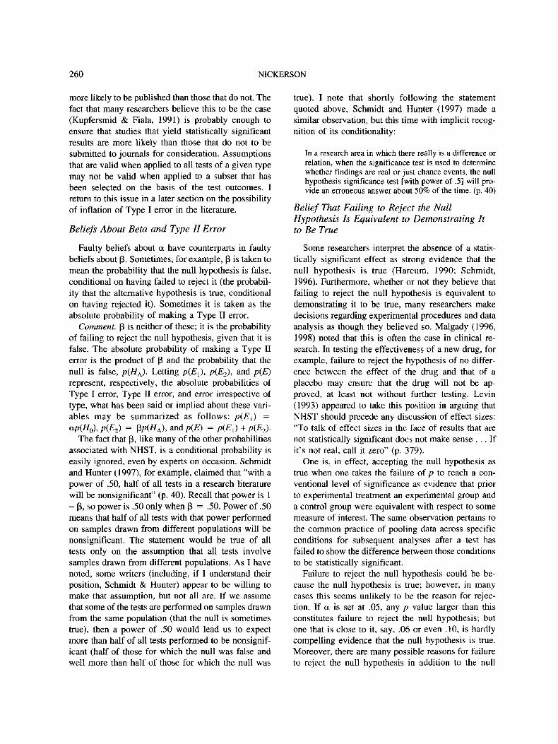
260 NICKERSON
more likely to be published than those that do not. The
fact that many researchers believe this to be the case
(Kupfersmid & Fiala, 1991) is probably enough to
ensure that studies that yield statistically significant
results are more likely than those that do not to be
submitted to journals for consideration. Assumptions
that are valid when applied to all tests of a given type
may not be valid when applied to a subset that has
been selected on the basis of the test outcomes. I
return to this issue in a later section on the possibility
of inflation of Type I error in the literature.
Beliefs About Beta and Type II Error
Faulty beliefs about a have counterparts in faulty
beliefs about p. Sometimes, for example, p is taken to
mean the probability that the null hypothesis is false,
conditional on having failed to reject it (the probabil-
ity that the alternative hypothesis is true, conditional
on having rejected it). Sometimes it is taken as the
absolute probability of making a Type II error.
Comment, p is neither of these; it is the probability
of failing to reject the null hypothesis, given that it is
false. The absolute probability of making a Type II
error is the product of p and the probability that the
null is false, p(HA). Letting p(Et), p(E2), and />(£)
represent, respectively, the absolute probabilities of
Type I error, Type II error, and error irrespective of
type, what has been said or implied about these vari-
ables may be summarized as follows: p(E,) —
ap(H0),p(E2) = p/>(«A), and/>(£) = p(E,) + p(E2).
The fact that p, like many of the other probabilities
associated with NHST, is a conditional probability is
easily ignored, even by experts on occasion. Schmidt
and Hunter (1997), for example, claimed that "with a
power of .50, half of all tests in a research literature
will be nonsignificant" (p. 40). Recall that power is 1
- P, so power is .50 only when p = .50. Power of .50
means that half of all tests with that power performed
on samples drawn from different populations will be
nonsignificant. The statement would be true of all
tests only on the assumption that all tests involve
samples drawn from different populations. As I have
noted, some writers (including, if I understand their
position, Schmidt & Hunter) appear to be willing to
make that assumption, but not all are. If we assume
that some of the tests are performed on samples drawn
from the same population (that the null is sometimes
true), then a power of .50 would lead us to expect
more than half of all tests performed to be nonsignif-
icant (half of those for which the null was false and
well more than half of those for which the null was
true). I note that shortly following the statement
quoted above, Schmidt and Hunter (1997) made a
similar observation, but this time with implicit recog-
nition of its conditionality:
In a research area in which there really is a difference or
relation, when the significance test is used to determine
whether findings are real or just chance events, the null
hypothesis significance test [with power of .5] will pro-
vide an erroneous answer about 50% of the time. (p. 40)
Belief That Failing to Reject the NullHypothesis Is Equivalent to Demonstrating Itto Be True
Some researchers interpret the absence of a statis-
tically significant effect as strong evidence that the
null hypothesis is true (Harcum, 1990; Schmidt,
1996). Furthermore, whether or not they believe that
failing to reject the null hypothesis is equivalent to
demonstrating it to be true, many researchers make
decisions regarding experimental procedures and data
analysis as though they believed so. Malgady (1996,
1998) noted that this is often the case in clinical re-
search. In testing the effectiveness of a new drug, for
example, failure to reject the hypothesis of no differ-
ence between the effect of the drug and that of a
placebo may ensure that the drug will not be ap-
proved, at least not without further testing. Levin
(1993) appeared to take this position in arguing that
NHST should precede any discussion of effect sizes:
"To talk of effect sizes in the face of results that are
not statistically significant does not make sense . . . If
it's not real, call it zero" (p. 379).
One is, in effect, accepting the null hypothesis as
true when one takes the failure of p to reach a con-
ventional level of significance as evidence that prior
to experimental treatment an experimental group and
a control group were equivalent with respect to some
measure of interest. The same observation pertains to
the common practice of pooling data across specific
conditions for subsequent analyses after a test has
failed to show the difference between those conditions
to be statistically significant.
Failure to reject the null hypothesis could be be-
cause the null hypothesis is true; however, in many
cases this seems unlikely to be the reason for rejec-
tion. If a is set at .05, any p value larger than this
constitutes failure to reject the null hypothesis; but
one that is close to it, say, .06 or even .10, is hardly
compelling evidence that the null hypothesis is true.
Moreover, there are many possible reasons for failure
to reject the null hypothesis in addition to the null
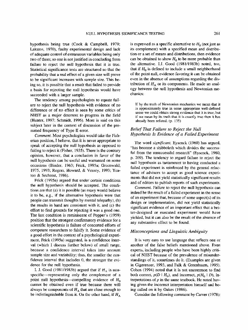
NULL HYPOTHESIS SIGNIFICANCE TESTING 261
hypothesis being true (Cook & Campbell, 1979;
Lakatos, 1970), faulty experimental design and lack
of adequate control of extraneous variables being only
two of them; so one is not justified in concluding from
failure to reject the null hypothesis that it is true.
Statistical significance tests are structured so that the
probability that a real effect of a given size will prove
to be significant increases with sample size. This be-
ing so, it is possible that a result that failed to provide
a basis for rejecting the null hypothesis would have
succeeded with a larger sample.
The tendency among psychologists to equate fail-
ure to reject the null hypothesis with evidence of no
difference or of no effect is seen by some critics of
NHST as a major deterrent to progress in the field
(Hunter, 1997; Schmidt, 1996). More is said on this
subject later in the context of discussion of the pre-
sumed frequency of Type II error.
Comment. Most psychologists would take the Fish-
erian position, I believe, that it is never appropriate to
speak of accepting the null hypothesis as opposed to
failing to reject it (Fisher, 1935). There is the contrary
opinion, however, that a conclusion in favor of the
null hypothesis can be useful and warranted on some
occasions (Binder, 1963; Frick, 1995a; Greenwald,
1975, 1993; Rogers, Howard, & Vessey, 1993; Yea-
ton & Securest, 1986).
Frick (1995a) argued that under certain conditions
the null hypothesis should be accepted. The condi-
tions are that (a) it is possible (as many would believe
it to be, e.g., if the alternative hypothesis were that
people can transmit thoughts by mental telepathy), (b)
the results in hand are consistent with it, and (c) the
effort to find grounds for rejecting it was a good one.
The last condition is reminiscent of Popper's (1959)
position that the strongest confirmatory evidence for a
scientific hypothesis is failure of concerted efforts of
competent researchers to falsify it. Some evidence of
a good effort in the context of a psychological experi-
ment, Frick (1995a) suggested, is a confidence inter-
val (which I discuss further below) of small range,
because a confidence interval takes into account
sample size and variability; thus, the smaller the con-
fidence interval that includes 0, the stronger the evi-
dence for the null hypothesis.
I. J. Good (1981/1983b) argued that if HA is non-
specific—representing only the complement of a
point null hypothesis—compelling evidence of H0
cannot be obtained even if true because there will
always be components of HA that are close enough to
be indistinguishable from it. On the other hand, if HA
is expressed as a specific alternative to H0 (not just as
its complement) with a specified mean and distribu-
tion or a set of means and distributions, then evidence
can be obtained to show //„ to be more probable than
the alternative. I.J. Good (1981/1983b) noted, too,
that if H0 is defined to include a small neighborhood
of the point null, evidence favoring it can be obtained
even in the absence of assumptions regarding the dis-
tribution of HA or its components. He made an anal-
ogy between the null hypothesis and Newtonian me-
chanics:
If by the truth of Newtonian mechanics we mean that itis approximately true in some appropriate well-definedsense we could obtain strong evidence that it is true; butif we mean by its truth that it is exactly true then it hasalready been refuted, (p. 135)
Belief That Failure to Reject the NullHypothesis Is Evidence of a Failed Experiment
The word significant, Eysenck (1960) has argued,
"has become a shibboleth which divides the success-
ful from the unsuccessful research" (Eysenck, 1960,
p. 269). The tendency to regard failure to reject the
null hypothesis as tantamount to having conducted a
failed experiment is reinforced by the general reluc-
tance of advisors to accept as good science experi-
ments that did not yield statistically significant results
and of editors to publish reports of such experiments.
Comment. Failure to reject the null hypothesis can
indeed be the result of a failed experiment in the sense
of an experiment that, because of some aspect(s) of its
design or implementation, did not yield statistically
significant evidence of an important effect that a bet-
ter-designed or executed experiment would have
yielded, but it can also be the result of the absence of
any substantive effect to be found.
Misconceptions and Linguistic Ambiguity
It is very easy to use language that reflects one or
another of the false beliefs mentioned above. Even
experts, including people who have been highly criti-
cal of NHST because of the prevalence of misunder-
standings of it, sometimes do it. (Examples are given
in Gigerenzer, 1993, and Falk & Greenbaum, 1995).
Cohen (1994) noted that it is not uncommon to find
both correct, p(D I H0), and incorrect, p(H0 I D), in-
terpretations of p in the same textbook. He noted hav-
ing given the incorrect interpretation himself and be-
ing called on it by Oakes (1986).
Consider the following comment by Carver (1978):
262 NICKERSON
Properly interpreted, statistical significance testing pro-vides a p value or the probability of obtaining meandifferences of given sizes under the null hypothesis.Thus, the p value may be used to make a decision aboutaccepting or rejecting the idea that chance caused theresults. (Carver, 1978, p. 387)
The first of these statements equates p with p(D I H0);
the second seems to imply that p can be used to infer
the probability that the null is true. As pointed out in
the foregoing, without a knowledge of p(D I H/J or of
some assumption regarding its value, the value of p
does not constitute an adequate basis for inferring
whether a particular result was obtained by chance.
The value of p tells us the probability that a chance
process would have yielded such a result, but without
knowing the probability that a nonchance process
would have yielded it and without knowing the prior
probabilities, p(HQ) andp(HA), we do not have what is
needed to compute the probability that this particular
result was produced by chance.
Falk and Greenbaum (1995) pointed to verbal am-
biguity as a major factor contributing to widespread
misconceptions about NHST, especially confusions
involving conditional probabilities. Linguistic ambi-
guity and unstated assumptions have been noted as
problematic to the understanding of probabilistic re-
lationships more generally (Bar-Hillel & Falk, 1982;
Falk, 1992; Gillman, 1992; Margolis, 1987; Nicker-
son, 1996). The distinction between p(D I H) andpfH
I D) appears to be one that is especially easily ob-
scured by casual language use.
Consider the expressions "the probability of obtain-
ing D by chance" and "the probability that D was
obtained by chance." It would hardly be surprising if
these expressions were taken by most people to have
the same referent. However, if what is meant by the
first is "the probability that a process known to be a
chance process, call it H, will produce D" and what is
meant by the second is "the probability that a known
event, D, was produced by a chance process, H" they
are quite different. The first is a reference to p(D I H),
and the second to p(H I D).
It is also easy to find casual expressions of proba-
bilistic relationships that lend themselves to more than
one interpretation. "The probability that a chance pro-
cess will produce D," for example, can be taken to
mean "given a chance process, the probability that it
will produce D"; but it could also mean "the prob-
ability that a chance process will occur and will pro-
duce D." Again, letting H represent the chance pro-
cess, the first expression can be represented as p(D I
H), and the second as p(H & D) or p(H)p(D I H).
Alternatively, consider the definition of power as "the
probability of correctly rejecting the null hypothesis"
(Harlow, 1997, p. 6). Power is the probability of re-
jecting the null hypothesis, given that it is false. "The
probability of correctly rejecting the null hypothesis"
might be interpreted to mean this, but it could also be
taken to mean the absolute probability of correctly
rejecting the null hypothesis, which is to say the joint
probability of the null hypothesis being false and it
being rejected. (In the context of computer simulation
research, this ambiguity is sometimes avoided by re-
ferring to power as the proportion of false null hy-
potheses rejected [Lashley & Bond, 1997].)
I believe that much of the confusion about NHST
and about what p values mean derives from such am-
biguities in casual language, some of which can be
quite subtle. Although I have tried not to make state-
ments in this article that are ambiguous or that reflect
the beliefs that I am claiming are incorrect, I am far
from confident that I have been successful in this
regard.
Summary Regarding Misconceptions
The burden of the present article to this point has
been to argue that there are many ways in which
NHST can be, and is, misunderstood. Most, if not all,
of the false beliefs mentioned here have been noted
before, in some cases by many writers (e.g., Carver,
1978; Oakes, 1986; Schmidt, 1996). Investigators
have documented misinterpretations in numerous
published research articles (Dar, Serlin, & Omer,
1994) and in widely used texts as well (Cohen, 1994;
Huberty, 1993).
Many of the conceptual difficulties that people
have with NHST have their roots, I believe, in a fail-
ure to distinguish between absolute and conditional
probabilities and, in particular, in failure to under-
stand that the value of p produced by conventional
tests of statistical significance is a conditional prob-
ability—the probability of getting the obtained statis-
tical result on the assumption that the null is true. A
further source of confusion is failure to distinguish
between the two conditional probabilities p(D I H0)
and p(Ha I D), and treatment of the former as though
it were the latter. Similar confusions pertain to a,
which is often treated as the absolute probability of a
Type I error, or as the conditional probability of a
Type I error given that the null has been rejected,
when in fact it is the probability of a Type I error
NULL HYPOTHESIS SIGNIFICANCE TESTING 263
conditional on the null being true. Comparable points
can be made regarding fj.
If there is an additional key insight in understand-
ing what NHST does and does not do, I think it is
recognition that p(D I H0) tells us nothing about the
value oip(D I HA) and, in particular, that p(D I #A) is
not the complement of p(D I H0). If p(H0) andp(HA)
are complements, then p(//A) = 1 - p(Ha) and p(HA
I D) — 1 - p(Ha I D). However, it is not necessarily
the case \haip(D I HA) = 1 -p(D I H0). Theoretically,
both p(D I HA) and p(D I H0) can vary from 0 to 1
independently. In particular, both p(D I H0) and p(D I
Hf) can be very small, and it is possible forp(D I HA)
to be smaller than p(D I H 0 ) when they are both small.
The latter possibility is the basis of Lindley's paradox,
described above.
I strongly suspect that many people believe that
p(D I H0) and p(D I HA) are complements, or at least
that if p(D I Hu) is small, p(D I HA) must be large. If
either of these relationships pertained, many of the
beliefs that I have described as false would be true.
Neither of these relationships necessarily pertains; in
many cases of interest, it may be reasonable to assume
that p(D I Hf) is greater than p(D I H0) or even that
p(D I Hf) is much greater thas\p(D I H0), but this is an
assumption; seldom is it possible to specify p(D I HA)
precisely. Moreover, as Edwards (1965) has pointed
out, typically in classical statistics the alternative to
the null hypothesis is undefined, and attaching a prob-
ability conditional on an undefined hypothesis is sel-
dom easy to do.
Lindley (1977) argued that when the probability of
the data is small under both hypotheses under consid-
eration, it makes sense to wonder whether perhaps
some other hypothesis should be considered. DeGroot
(1982) also noted that making an observation that is
improbable under both hypotheses is likely to cause
one to feel that there may be a good explanation of the
observation other than those considered and to rethink
one's prior distribution of probabilities. On the other
hand, in another context Lindley (1982) pointed out
that "the comparison of small probabilities is the usual
situation because most things that happen to us have
low probability; we go through life experiencing rare
events" (p. 335). In isolation, the fact that an event has
low probability tells us very little about the nature of
its cause.
To say that a result is statistically significant is to
say that the probability of obtaining that result if there
were no factors operating but chance is small. How-
ever, because the probability of obtaining that result
in any case—by chance or otherwise—could be small,
to say that a result is statistically significant is to say
nothing conclusive about the probability that particu-
lar result was produced by chance. If one is willing to
make the assumption thatp(D I HA) is large relative to
p(D I H0), then one has a legitimate basis for inter-
preting a small p as evidence for increasing the like-
lihood of HA relative to that of H0. Perhaps this as-
sumption underlines many applications of NHST, but
seldom does one see an explicit acknowledgment
of it.
Other Criticisms of NHST
Not all the criticisms that have been directed at
NHST have focused on false beliefs about what it
means, although many of them have. We turn now to
some of the criticisms of other types that have been
made.
A Priori Unlikelihood That the Null HypothesisIs True
The reasonableness of NHST has been challenged
by many writers on the grounds that the null hypoth-
esis is very unlikely ever to be true and that statisti-
cally significant (though not necessarily large) differ-
ences (from 0 or any other hypothesized value) are
almost assured on practically any dimension if one
uses sufficiently large samples (Bakan, 1966; Berk-
son, 1938; Cohen, 1990; Grant, 1962; Hodges &
Lehmann, 1954; Lindgren, 1976; Meehl, 1967, 1978;
Murphy, 1990; Neyman & Pearson, 1928a, 1928b;
Nunnally, 1960). The claim is that generally when an
experiment yields data that do not permit the rejection
of the null hypothesis at a prescribed level of statis-
tical significance, it can be assumed that a significant
difference would be obtained simply by increasing the
sample size (Hays, 1994; Nunnally, 1960; Oakes,
1986). Thompson (1998) characterized the situation
this way: "Statistical testing becomes a tautological
search for enough participants to achieve statistical
significance. If we fail to reject, it is only because
we've been too lazy to drag in enough participants"
(p. 799). Meehl (1990b, 1997) argued that the finding
of significant correlations of nontrivial size between
arbitrary variables with large data sets should not be
surprising because everything really is related, to
some degree, to everything else.
Not all psychologists agree with the claim that the
null hypothesis is never true. Some have argued that
demonstrating the tenability of the null hypothesis is
264 NICKERSON
as legitimate a goal of research, though not necessar-
ily as easily attained, as is demonstrating the tenabil-
ity of any alternative hypothesis (Chow, 1996; Prick,
I995a), Frick (1995a), for example, argued that the
null hypothesis can be true and should sometimes be
accepted as such: "The null hypothesis is a valuable
claim that psychology should want to accept, not
merely fail to reject" (p. 132). Frick (1995a) conceded
that there are instances in which the null hypothesis
must be considered impossible but argued that this
should not preclude its use in cases for which it is
appropriate.
A context in which the possibility of obtaining evi-
dence that the null hypothesis is true or nearly so is of
considerable interest is medicine, as well as closely
related areas (Malgady, 1998). Bartko (1991) gave
several references in the biostatistics literature about
"proving" the null hypothesis. Statistical approaches
designed to establish the approximate equality (equal-
ity for practical purposes) of methods (as distinct from
establishing the superiority of one over the other) that
are based on classical NHST have been developed
(Hauck & Anderson, 1986; Rogers et al., 1993; West-
lake, 1988). These approaches are intended especially
for use in the context of pharmaceutical research,
where it is often important to establish that a new drug
does not have undesirable side effects or to determine
whether one drug or treatment is as clinically effective
as another (despite, say, differences in cost, conve-
nience, or other factors).
Hagen (1997) countered the claim that the null hy-
pothesis is almost always false by contending that it is
based on a misinterpretation of the null hypothesis.
The null hypothesis says nothing about samples beingequal, nor does the alternative hypothesis say that theyare different. Rather, when addressing group differences,the null hypothesis says that the observed samples, giventheir differences, were drawn from the same population,and the alternative hypothesis says that they were drawnfrom different populations, (p. 20)
Samples will always (or very nearly always) differ
with respect to any measurable variable of interest,
but this is true even of samples drawn from the same
population; so the fact that they differ with respect to
a specific measure in any particular instance is not
evidence that they were drawn from different popu-
lations. Only if the magnitude of the difference is
sufficiently great relative to the standard error of the
difference to meet a conventional criterion will the
conclusion that the samples are from different popu-
lations be drawn, and when samples really are drawn
from the same population the likelihood that the null
hypothesis will be rejected does not go to 1 as sample
size increases. As Hagen said:
We have been taught that a sufficiently large N willdetect differences no matter how tiny they may be. Butwhat we may forget is that small differences will alwaysbe detected by a large A^ only under the alternative hy-pothesis, not under the null. When samples are drawnfrom the same population, the variance of absolute dif-ferences between or among such samples will becomesmaller as N becomes larger. This diminishing varianceis reflected in a decrease in the variance of the particulartest statistic from which we draw our sample statistic.Accordingly, Type-I error remains roughly constant nomatter how large N becomes, (p. 20)
Another interpretation of the claim that the null
hypothesis is almost always false is that any experi-
mental manipulation—for example, differential treat-
ment of two groups—is bound to have some effect,
however small (Tukey, 1991). Hagen's counter to this
claim is that although it may be that differential treat-
ment will always have some effect, it may not have an
effect on the dependent variable of interest, and it is
only such an effect that will lead to rejection of the
null hypothesis.
Another response to the claim that the null hypoth-
esis is always or almost always false is that indepen-
dent of the validity or invalidity of the claim, what is
true of point null hypotheses need not be true of
"small interval" hypotheses that can be approximated
realistically by point nulls (Berger & Sellke, 1987;
Hodges & Lehmann, 1954; Serlin & Lapsley, 1985;
Wilson et al., 1967). More specifically, the argument
is that even if the probability of a true point null were
vanishingly small, something close to a null result—
an almost-null result—would not be impossible a
priori and for many purposes the null may serve as a
useful proxy for an almost-null hypothesis:
Although we may specify a point null hypothesis for thepurpose of our statistical test, we do recognize a more orless broad indifference zone about the null hypothesisconsisting of values which are essentially equivalent tothe null hypothesis for our present theory or practice.(Binder, 1963, p. 110)
Alternatively, as Meehl (1997) has said:
In practical contexts, when we have sufficient power (1- p) so that there is not too big an asymmetry in thevalues of error rates « and p, we do want to make the"quasi-null" inference, not that H0 as a precise point
NULL HYPOTHESIS SIGNIFICANCE TESTING 265
value is literally true, but that something close to it is. (p.395)
It has been argued that in most experiments in
which the null hypothesis is tested the investigator is
not really interested in the possibility of precisely zero
effect but rather in whether whatever effect there
might be is close enough to zero to be of no interest
(Rindskopf, 1997). As to why, if this is the case,
experimenters do not regularly test composite or
range null hypotheses rather than point nulls, Rind-
skopf surmised that testing a point null is the much
simpler process; although efforts to facilitate testing
range nulls, which require assumptions about the dis-
tribution of a statistic when the null is false, have been
made (e.g., Serlin & Lapsley, 1985, 1993). In the
meantime, if sample size is not so large as to ensure
detection of even negligibly small effects, testing of a
point null hypothesis is likely to yield roughly the
same result as would the testing of a small-range null.
Sensitivity ofNHST to Sample Size
Although the likelihood that a true null hypothesis
will be rejected does not increase with the sizes of the
samples compared, the likelihood that a real differ-
ence of a given magnitude will result in rejection of
the null hypothesis at a given level of confidence
does. It is also the case that the smaller a real differ-
ence is, the larger the samples are likely to have to be
to provide a basis for rejecting the null. In other
words, whether or not one assumes that the null hy-
pothesis is always or almost always false, when it is
false the probability that a statistical significance test
will lead to rejection increases with sample size.
This sensitivity to sample size has been the focus of
some of the sharpest criticisms of NHST (Bakan,
1966; McNemar, 1960; Nunnally, 1960; Thompson,
1998). It means that conclusions drawn from experi-
ments often depend on decisions experimenters have
made regarding how many participants to run. Also,
inasmuch as even very small real differences will be
detected by sufficiently large samples, it is possible
with very large samples to demonstrate statistical sig-
nificance for differences that are too small to be of
any theoretical or practical interest.
Because of the sensitivity of statistical significance
to sample size, the practice of increasing the size of
one's sample after performing an experiment that
yielded a difference that failed to attain significance is
generally considered poor form. As several writers
have pointed out, if one is permitted to use an optional
stopping rule, one can be quite certain of rejecting
even a true null hypothesis if one goes on sampling
for a sufficiently long time (I.J. Good, 1981/1983b;
Greenwood, 1938; Robbins, 1952). The experimenter
in this situation is somewhat like the gambler who is
free to specify the size of the wager on every bet and
to terminate the betting whenever he or she likes,
thereby being effectively assured of winning.
The importance of being specific about the
sample(s) one intends to use for experimental pur-
poses is illustrated by the following situation, adapted
from Berger and Berry (1988). Suppose an experi-
menter were to say, "I have just tossed a coin 17
times, obtaining 13 heads and 4 tails. Should I reject
the null hypothesis (of an unbiased coin), and if so at
what level of confidence?" One cannot answer this
question without knowing the experimenter's original
intent. If the intent were to toss the coin 17 times and
make a statistical decision on the basis of the out-
come, the answer provided by the standard approach
to NHST is that the null hypothesis should be rejected
at a confidence level of approximately .05. If, on the
other hand, the experimenter had intended to toss the
coin until 4 heads and 4 tails had been obtained, and
the 4th tail happened to occur on the 17th toss, the
null hypothesis should be rejected at a confidence
level of .02.
The reason one gets two results from the sample is
that although the sample is the same, it is drawn from
two different populations. In the first case the popu-
lation is all possible sets of 17 coin tosses; in the
second the population is all possible sequences of
tosses that are terminated on the first toss for which it
is true that at least 4 of each possible outcome (heads
or tails) have occurred. This population includes se-
quences ranging in number from 8 to infinity. Berger
and Berry (1988) argued that standard statistical
methods, which include NHST, "depend on the inten-
tions of the investigator, including intentions about
data that might have been obtained but were not" (p.
159).
Lindley (1993) made a similar point with respect to
a modified form of Fisher's (1935) famous tea-tasting
experiment. Suppose a tea taster, who claims to be
able to tell by tasting a cup of tea with milk whether
the tea or milk was put in the cup first, is tested six
times and is right on the first five tries and wrong on
the sixth: RRRRRW. The usual way of judging
whether performance this good is likely on the basis
of chance is to ask what the probability of getting five
or more correct in six tries is; the answer, as conven-
266 NICKERSON
tionally calculated, is .109, which assumes a sample
space that includes all possible outcomes of 6 tests.
However, suppose the experimenter's intent was to
continue the trials as long as the tea taster's answers
were correct—to terminate it after the first wrong re-
sponse. In this case the sample space includes infi-
nitely many sequences, and the probability of getting
five or more correct responses before the first error is
.031.
Lindley (1993) used this illustration of the ambi-
guity of the concept of outcomes that are more ex-
treme than a specified outcome as a basis for arguing
for the abandonment of the use of more extreme out-
comes in statistical analyses—as when in NHST one
considers the probability of obtaining a result equal to
or more extreme than the one obtained. Inasmuch as
he had already argued that considering only the prob-
ability of the exact outcome obtained is unsatisfactory
because in some experiments the probability of every
possible outcome is small, he then went on to argue
that the better way to evaluate an outcome is the
Bayesian approach of considering its probability con-
ditional on the null hypothesis relative to its probabil-
ity conditional on one or more alternative hypoth-
eses—which is to say, likelihood ratios. Unlike the
use of NHST, however, the use of the Bayesian ap-
proach requires that one or more alternatives to the
null hypothesis and the probability of the data condi-
tional on it (them) be specified. As Lindley (1993)
said:
The Bayesian method is comparative. It compares theprobabilities of the observed event on the null hypothesisand on the alternatives to it. In this respect it is quitedifferent from Fisher's approach which is absolute in thesense that it involves only a single consideration, the nullhypothesis, (p. 25; see also Lindley, 1984)
Perhaps in part to preclude the use of strategies that
permit an experimenter to decide on sample size on
the basis of how an experiment in progress was turn-
ing out, some have argued that an investigator must
specify experimental details—sample size, statistical
tests, significance levels, interpretations of possible
outcomes—in advance of collecting data. Fisher
(1935/1956) expressed this idea as follows:
In considering the appropriateness of any proposed ex-perimental design, it is always needful to forecast allpossible results of the experiment, and to have decidedwithout ambiguity what interpretation shall be placedupon each one of them. Further, we must know by whatargument this interpretation is to be sustained, (p. 1512)
I. J. Good (1976/1983a) has challenged this posi-
tion:
Many elementary textbooks recommend that test criteriashould be chosen before observations are made. Unfor-tunately this could lead to a data analyst missing someunexpected and therefore probably important feature ofthe data. There is no existing substitute for examiningthe original observations with care. This is often morevaluable than the application of formal significance tests.If it is easy and inexpensive to obtain new data, thenthere is little objection to the usual advice, since theoriginal data can be used to formulate hypotheses to betested on later samples. But often a further sample isexpensive or virtually impossible to obtain, (p. 51) It'smisleading to tell a student he must decide on his sig-nificance test in advance, although it is correct accordingto the Fisherian technique, (p. 54)
I. J. Good (1981/1983b) argued that "one cannot al-
ways sensibly determine a significance test in advance
because, heretical though it may be in some quarters,
sometimes the data overwhelmingly suggest a sen-
sible theory after the data are examined" (p. 145).
There are techniques for analyzing data sequen-
tially that are widely recognized to be legitimate that
do not require the advance specification of sample
size (Wald, 1945, 1947/1974). Bayesian approaches
to belief revision are in this category. For the most
part, such techniques are alternatives to NHST, but
some work on application of sequential stopping rules
to NHST has been done (Frick, 1998).
It can be argued that the question of the extent to
which the details of a null hypothesis test should be
specified in advance is beside the point. If, as some
believe, we know before collecting data that the null
hypothesis is false and that a sufficiently large sample
would show it to be so in any particular case, what is
the purpose of doing a test at all (Cohen, 1990; Ney-
man & Pearson, 1928a, 1928b; Nunnally, I960)? If
the null hypothesis is never true, then evidence that it
should be rejected in any particular instance is neither
surprising nor useful.
I. J. Good's (1956/1983c) answer to the question of
why one would want to do a significance test is, 'That
we wish to test whether the hypothesis is in some
sense approximately true, or whether it is rejectable
on the sort of size of sample that we intend to take" (p.
62). This point, he noted, is not usually made clear in
textbooks on statistics, and in any event never formu-
lated precisely. A similar answer has been given by
Mulaik, Raju, and Harshman (1997):
NULL HYPOTHESIS SIGNIFICANCE TESTING 267
It doesn't matter if the null hypothesis is always judgedfalse at some sample size, as long as we regard this as anempirical phenomenon. What matters is whether at thesample size we have we can distinguish observed devia-tions from our hypothesized values to be sufficientlylarge and improbable under a hypothesis of chance thatwe can treat them reasonably but provisionally as notdue to chance error, (p. 80)
However, the more compelling response to the
question of why to do a statistical significance test is
denial of the claim that we know before doing an
experiment that the outcome will be rejection of the
null, if only the sample is sufficiently large. The ar-
gument, noted in the preceding section, that if the
samples being compared are drawn from the same
population with respect to the parameter of interest,
the probability of getting a significant difference with
respect to that parameter does not go to 1 as the
sample size increases, seems to me conclusive.
Faulty Logic
Berkson (1942) criticized NHST on the grounds
that it is illogical. Commenting on a textbook presen-
tation of the null hypothesis procedure in which it was
argued that the observation of a difference that would
seldom occur by chance casts much doubt on the hy-
pothesis of no difference, he described the case this
way:
Consider [the argument] in syllogistic form. It says "If Ais true, B will happen sometimes; therefore if B has beenfound to happen, A can be considered disproved." Thereis no logical warrant for considering an event known tooccur in a given hypothesis, even if infrequently, as dis-proving the hypothesis, (p. 326)
In fairness to the textbook writer, the claim was not
that the observed result proved the null hypothesis to
be false, but only that it cast much doubt on it. And in
fairness to Berkson (1942), it needs to be said that his
major complaint against NHST was that the logic of it
"does not seem to accord with what would be the
mode of reasoning in ordinary rational discourse, nor
with the rationale of usual procedures as they are ob-
served in the scientific laboratory" (p. 326). Berkson
(1942) proposed the following principle as generally
operative in scientific inquiry:
The finding of an event which is frequent under a hy-pothesis H, can be taken as evidence in favor of H,. IfH0 is a contradictory alternative to H, for which theevent would not be frequent, then per corollary the find-ing of the event is, in so far, evidence in disfavor of Hu.(p. 327)
As applied to NHST, the principle means
If an event has occurred, the definitive question is not,"Is this an event which would be rare if H0 is true?" but"Is there an alternative hypothesis under which the eventwould be relatively frequent?" If there is no plausiblealternative at all, the rarity is quite irrelevant to a deci-sion, and if there is such an alternative, the decisivequestion is, "Would the event be relatively frequent?" (p.327)
This is similar to the claim that p(D I HQ) tells us
nothing about p(H0 I D) in the absence of knowledge
or of an assumption about p(D I #A). (Berkson, 1942,
also developed an argument for being willing to ac-
cept—as distinct from failing to reject—the null hy-
pothesis under specific conditions).
Cohen (1994) and Falk and Greenbaum (1995) con-
tended more generally that the modus tollens form of
argument—"If P then Q; not Q, therefore not P"—
which is valid with categorical premises, is invalid
when the premises are probabilistic: "If P then prob-
ably Q; not Q; therefore probably not P" ("If H0 is
true then probably p > .05;p< .05; therefore probably
HQ is false"). Again, the point is that in order to say
anything about the probability of H0 given the occur-
rence of an event that has low probability if H0 is true,
we need to know, or to assume something about, the
probability of the event if Hn is false.
McDonald (1997) also considered statistical tests to
be patterned after modus tollens: "If null hypothesis
(HQ) then not-these-data (not-D), but D, therefore not-
H0, [which in the statistical context becomes] if Hn
then D improbable (< a), therefore either not-//0 or
the improbable has occurred" (p. 200). McDonald
agreed with others who have pointed out that this does
not justify the conclusion that H0 is improbable or
unlikely, but he did allow that it may be rational
(though possibly erroneous) to conclude not-//0 rather
than to conclude that the improbable has occurred; the
choice here is between nol-H0 (the probability of
which is unknown) and an event whose probability is
known to be low.
Cortina and Dunlap (1997) acknowledged that mo-
dus tollens does not have the force with probabilistic
premises that it has with categorical ones, but they
argued that it can be used to good effect under certain
conditions. They contended that it is approximately
correct when the truth of the first premise's anteced-
ent is positively related to the truth of its consequent.
The claim is that the more nearly correct it is to con-
sider the antecedent of the conditional probabilistic
268 NICKERSON
premise to be a cause or reason for the consequent, the
more sense it makes to apply modus tollens. If the
consequent of the conditional premise is very likely to
be true, independent of the truth or falsity of the an-
tecedent, the form has little force. "If X, then that
person is probably not a member of Congress" seems
likely to be true, almost independently of what is sub-
stituted for X, so X cannot be considered a reason for
expecting the consequent to be true. This stands in
contrast to the statement "If the experimental manipu-
lation did not work, then p would probably be greater
than .05," which seems to be offering the experimen-
tal manipulation not working as a reason for getting a
value ofp greater than .05. Cortina and Dunlap argued
that the application of modus tollens is justified in the
latter case but not in the former; they suggested that
the latter case is the more representative than the
former of the conditions under which NHST is usually
done and concluded that "the typical approach to hy-
pothesis testing does not violate the relevant rule of
syllogistic reasoning to any great degree" (p. 166).
Hagen's (1997, 1998) position with respect to the
argument that NHST lacks logical validity is that "ar-
guments can be reasonable and defensible even when
they are not logically valid in a formal sense" (1997,
p. 22). I. J. Good (1982) also considered classical
NHST to be useful, despite being logically flawed:
"Logically there is something wrong with the use of
tail-area probabilities, but I still find them useful be-
cause of the well-known difficulties about priors in
the Bayesian position" (p. 342).
Noninformativeness of Test Outcomes
Another objection to NHST is that such tests pro-
vide relatively little information about the relationship
between the dependent and independent variables.
They do not, as we have seen, provide a measure of
the size of an effect, nor do they reveal the strength of
the relationship between dependent and independent
variables. They give evidence only of whether a sta-
tistically significant effect has been obtained and, if
so, of the direction of the effect. At least when the null
hypothesis is the hypothesis of zero difference (zero
effect, zero correlation), statistical significance pro-
vides at best evidence against the hypothesis of no
difference (effect, correlation), which is very little in-
formation indeed. As Abelson (1997b) has said,
"Typically, mere difference from zero is totally unin-
teresting" (p. 121).
In contrast, a regression analysis gives an indica-
tion of the degree of relatedness of variables (Cohen,
1977; Cohen & Cohen, 1983). The ratio of between-
treatments variance to total variance—the proportion
of total variance in a dependent variable that can be
attributed to treatments—has also been suggested as
an indication of strength of relationship between in-
dependent and dependent variables (R. Good &
Fletcher, 1981; Hays, 1994; Stocks, 1987). A Bayes-
ian analysis can provide a posterior probability for
each of a set of hypotheses of interest (Bakan, 1966;
Cronbach & Snow, 1977; but only, of course, if the
values of the variables required by the computation
are known or assumed).
Inappropriateness of All-or-None DecisionsRegarding Significance
Many writers object to the sharpness of the distinc-
tion that is made between significant and nonsignifi-
cant results (Eysenck, 1960; Frick, 1996; Glass,
McGaw, & Smith, 1981; Grant, 1962; Nunnally,
1960; Rossi, 1997; C. D. Wickens, 1998). According
to some interpretations of the conventional rules of
application of NHST, a result that yields a p value
only slightly greater than the a level is to be given the
same treatment as one that is much greater. Many
researchers find it very difficult to follow this prin-
ciple, however, and insist on distinguishing between
"marginally significant" and "nonsignificant" results.
It does seem a little strange to consider a difference
with a p of .05 to represent something real while
dismissing one with a p of .06 as due to chance.
Nevertheless, several inquiries into how psychologists
interpret the results of statistical significance tests
have shown a "cliff characteristic" at .05, according to
which reported confidence in a finding drops abruptly
when p becomes larger than this value (Beauchamp &
May, 1964; Rosenthal & Gaito, 1963, 1964); cliff
characteristics of lesser magnitude have also been
found for/; values of .01 and .10 (Minturn, Lansky, &
Dember, 1972; Nelson, Rosenthal, & Rosnow, 1986).
Rozeboom (1960) objected to NHST on the
grounds that it treats acceptance or rejection of a hy-
pothesis as though this were a decision one makes on
the basis of the experimental data; the experimenter's
task, he argued, is not that of making a binary decision
either to accept or to reject a tested hypothesis, but
rather that of determining how the experimental out-
come changes the probability that the hypothesis is
true. The scientist "is fundamentally and inescapably
committed to an explicit concern with the problem of
inverse probability" (p. 422). As a matter of fact, Ro-
zeboom (1960) contended, researchers do not apply
NULL HYPOTHESIS SIGNIFICANCE TESTING 269
the principles of NHST in forming and refining their
own beliefs about the tenability of hypotheses. 1. J.
Good (1981/1983b) made a similar point in contend-
ing that it is not always sensible either to accept or to
reject a hypothesis in a sharp sense. Rosnow and
Rosentbal (1989b) maintained that dichotomous sig-
nificance testing has no ontological basis and that the
strength of evidence for or against the null hypothesis
must be considered a fairly continuous function of the
magnitude of p.
The dichotornization of experimental results into
those that prove to be statistically significant and
those that do not, and the attendant strong bias for
publishing only the former, are seen by some critics of
NHST as very detrimental to the advance of psychol-
ogy as a science. Essentially ignoring null findings,
they argue, inhibits the accumulation of knowledge
across studies (Meehl, 1978; Rossi, 1997).
Arbitrariness of the Decision Criterion
Closely associated with the objection regarding the
sharp distinction between significance and nonsignifi-
cance is concern about the arbitrariness of the a cri-
terion (Glass et al., 1981; Rozeboom, 1960). The a
criterion that is most widely recommended is .05
(Cowles & Davis, 1982). The grip that this number
has had on the research community for decades has
been parodied by Rosnow and Rosenthal (1989b):
It may not be an exaggeration to say that for many Ph.D.
students, for whom the .05 alpha has acquired almost an
ontological mystique, it can mean joy, a doctoral degree,
and a tenure-track position at a major university if their
dissertation/? is less than .05. However, if the/) is greater
than .05, it can mean ruin, despair, and their advisor's
thinking of a new control condition that should be run.
(p. 1277)
My experience suggests that .05 is treated by many
researchers today as an upper bound on what should
be considered statistically significant, but relatively
few specify it as « in advance of collecting (or re-
porting) data and then report all results relative to that
criterion. More commonly, researchers report a vari-
ety of p values in the same study, although they typi-
cally refer only to those that are less than .05 as sta-
tistically significant.
The guidance provided to authors by the Publica-
tion Manual of the American Psychological Associa-
tion (4th ed.; American Psychological Association
[APA], 1994) allows considerable latitude in the se-
lection (or not) of an a level and the reporting of p
values. Whether this is a good idea has been a topic of
debate (Labovitz, 1968). Some writers have urged
that, at least when the results of statistical significance
tests are to be used as a basis for decisions that matter,
the costs and benefits associated with the various
ways of being right and wrong should be considered
in deciding what the null hypothesis should be and in
setting the a level (Cox, 1958; Neyman, 1942; Oakes,
1986; Skipper, Guenther, & Nass, 1967).
In contrast, others believe that freedom to select
one's own a level adds an undesirable element of
subjectivity to the process of hypothesis evaluation
(Frick, 1996) and permits different investigators to
draw conflicting conclusions from the same data
(Cox, 1977). Rozeboom (1960) captured this concern
this way: "Surely the degree to which a datum cor-
roborates or impugns a proposition should be inde-
pendent of the datum-assessor's personal temerity"
(p. 420). The establishment of a widely adhered-to
criterion, say, an a of .05, is seen by some as an
attempt at standardization in the interest of objectiv-
ity, as "an admittedly arbitrary attempt to standardize
a bias against alternative hypotheses ... a deliberate
attempt to offer a standardized, public method for
objectifying an individual scientist's willingness to
make an inference" (W. Wilson et al., 1967, p. 191).
W. Wilson et al. contended that this approach is more
objective and less subject to variability deriving from
individual differences in belief states among experi-
menters than a Bayesian approach that requires the
assignment of personal probabilities would be. Chow
(1998a) defended the use of a strict a criterion by
arguing that it is analogous in importance to the main-
tenance by a teacher of a passing grade.
Test Bias
The question of bias in NHST is an interesting one,
in part because the convention of selecting a small a
is generally viewed as reflective of a strong bias
against rejection of a true null hypothesis. It has been
argued, however, that classical NHST (in contrast to
Bayesian tests) is in fact strongly biased against ac-
ceptance (or nonrejection) of the null hypothesis (Ed-
wards, 1965; Edwards et al., 1963; Lindley, 1993):
"Classical procedures quite typically are, from a
Bayesian point of view, far too ready to reject null
hypotheses" (Edwards et al., 1963, p. 225).
The bias against acceptance of the null hypothesis
of which Edwards and his colleagues (Edwards, 1965;
Edwards et al., 1963) spoke has been noted in this
article in the context of the discussion of the false
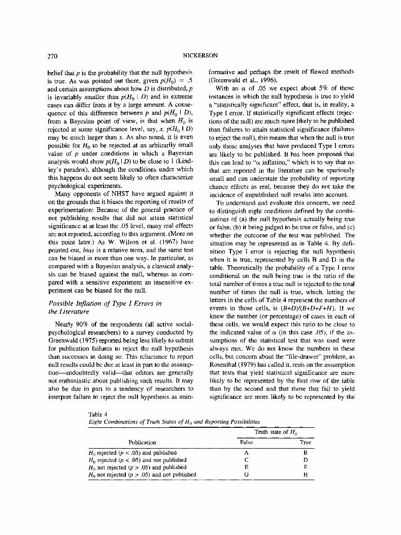
270 NICKERSON
belief that p is the probability that the null hypothesis
is true. As was pointed out there, given p(H0) = .5
and certain assumptions about how D is distributed, p
is invariably smaller than p(H0 I D) and in extreme
cases can differ from it by a large amount. A conse-
quence of this difference between p and p(H0 I D),
from a Bayesian point of view, is that when H0 is
rejected at some significance level, say, x, p(H0 I D)
may be much larger than x. As also noted, it is even
possible for HQ to be rejected at an arbitrarily small
value of p under conditions in which a Bayesian
analysis would show p(//0 I D) to be close to 1 (Lind-
ley's paradox), although the conditions under which
this happens do not seem likely to often characterize
psychological experiments.
Many opponents of NHST have argued against it
on the grounds that it biases the reporting of results of
experimentation: Because of the general practice of
not publishing results that did not attain statistical
significance at at least the .05 level, many real effects
are not reported, according to this argument. (More on
this point later.) As W. Wilson et al. (1967) have
pointed out, bias is a relative term, and the same test
can be biased in more than one way. In particular, as
compared with a Bayesian analysis, a classical analy-
sis can be biased against the null, whereas as com-
pared with a sensitive experiment an insensitive ex-
periment can be biased for the null.
Possible Inflation of Type I Errors inthe Literature
Nearly 90% of the respondents (all active social-
psychological researchers) to a survey conducted by
Greenwald (1975) reported being less likely to submit
for publication failures to reject the null hypothesis
than successes in doing so. This reluctance to report
null results could be due at least in part to the assump-
tion—undoubtedly valid—that editors are generally
not enthusiastic about publishing such results. It may
also be due in part to a tendency of researchers to
interpret failure to reject the null hypothesis as unin-
formative and perhaps the result of flawed methods
(Greenwald et al., 1996).
With an ct of .05 we expect about 5% of those
instances in which the null hypothesis is true to yield
a "statistically significant" effect, that is, in reality, a
Type I error. If statistically significant effects (rejec-
tions of the null) are much more likely to be published
than failures to attain statistical significance (failures
to reject the null), this means that when the null is true
only those analyses that have produced Type I errors
are likely to be published. It has been proposed that
this can lead to "a inflation," which is to say that as
that are reported in the literature can be spuriously
small and can understate the probability of reporting
chance effects as real, because they do not take the
incidence of unpublished null results into account.
To understand and evaluate this concern, we need
to distinguish eight conditions defined by the combi-
nations of (a) the null hypothesis actually being true
or false, (b) it being judged to be true or false, and (c)
whether the outcome of the test was published. The
situation may be represented as in Table 4. By defi-
nition Type I error is rejecting the null hypothesis
when it is true, represented by cells B and D in the
table. Theoretically the probability of a Type I error
conditional on the null being true is the ratio of the
total number of times a true null is rejected to the total
number of times the null is true, which, letting the
letters in the cells of Table 4 represent the numbers of
events in those cells, is (B+D)/(B+D+F+H). If we
knew the number (or percentage) of cases in each of
these cells, we would expect this ratio to be close to
the indicated value of a (in this case .05), if the as-
sumptions of the statistical test that was used were
always met. We do not know the numbers in these
cells, but concern about the "file-drawer" problem, as
Rosenthal (1979) has called it, rests on the assumption
that tests that yield statistical significance are more
likely to be represented by the first row of the table
than by the second and that those that fail to yield
significance are more likely to be represented by the
Table 4Eight Combinations of Truth States of H0 and Reporting Possibilities
Truth state of H0
Publication False
HO rejected (p < .05) and published AH0 rejected (p < .05) and not published C
H0 not rejected (p > .05) and published EHa not rejected (p > .05) and not published G
True
B
D
F
H
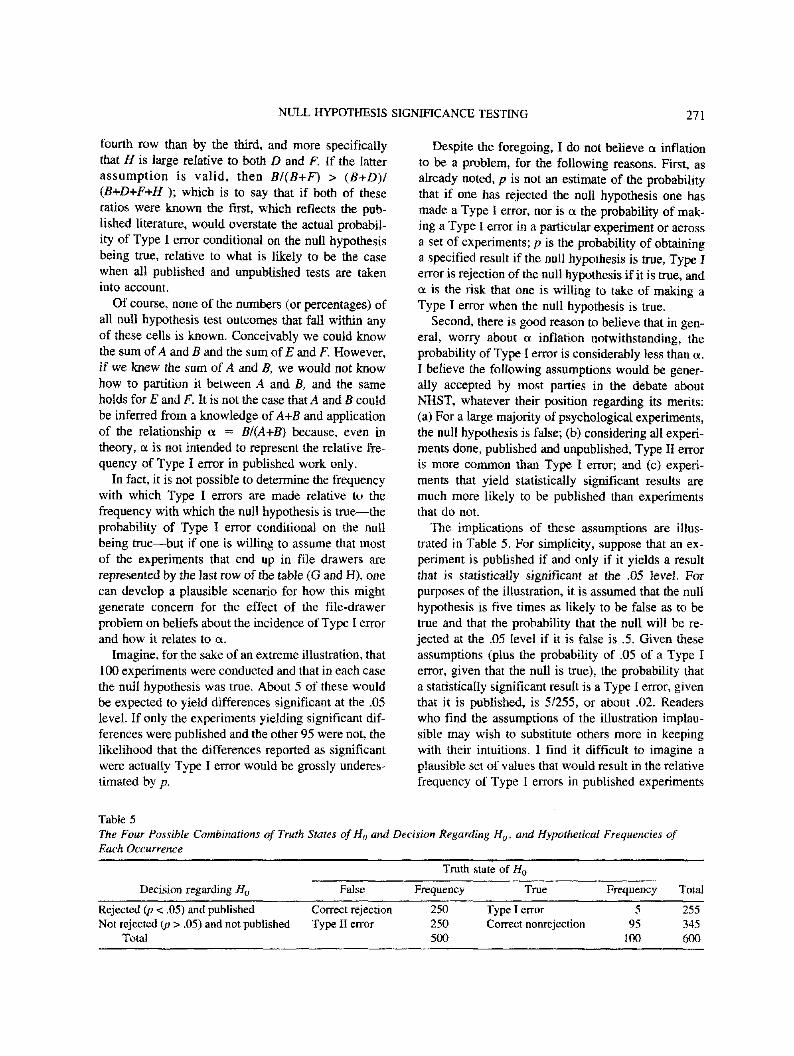
NULL HYPOTHESIS SIGNIFICANCE TESTING 271
fourth row than by the third, and more specifically
that H is large relative to both D and F. If the latter
assumption is valid, then B/(B+F) > (B+D)/
(B+D+F+H ); which is to say that if both of these
ratios were known the first, which reflects the pub-
lished literature, would overstate the actual probabil-
ity of Type I error conditional on the null hypothesis
being true, relative to what is likely to be the case
when all published and unpublished tests are taken
into account.
Of course, none of the numbers (or percentages) of
all null hypothesis test outcomes that fall within any
of these cells is known. Conceivably we could know
the sum of A and B and the sum of £ and F. However,
if we knew the sum of A and B, we would not know
how to partition it between A and B, and the same
holds for E and F. It is not the case that A and 8 could
be inferred from a knowledge of A+B and application
of the relationship a = B/(A+B) because, even in
theory, a is not intended to represent the relative fre-
quency of Type I error in published work only.
In fact, it is not possible to determine die frequency
with which Type I errors are made relative to the
frequency with which the null hypothesis is true—the
probability of Type I error conditional on the null
being true—but if one is willing to assume that most
of the experiments that end up in file drawers are
represented by the last row of the table (G and H), one
can develop a plausible scenario for how this might
generate concern for the effect of the file-drawer
problem on beliefs about the incidence of Type I error
and how it relates to a.
Imagine, for the sake of an extreme illustration, that
100 experiments were conducted and that in each case
the null hypothesis was true. About 5 of these would
be expected to yield differences significant at the .05
level. If only the experiments yielding significant dif-
ferences were published and the other 95 were not, the
likelihood that the differences reported as significant
were actually Type I error would be grossly underes-
timated by p.
Despite the foregoing, I do not believe a inflation
to be a problem, for the following reasons. First, as
already noted, p is not an estimate of the probability
that if one has rejected the null hypothesis one has
made a Type I error, nor is a the probability of mak-
ing a Type I error in a particular experiment or across
a set of experiments; p is the probability of obtaining
a specified result if the null hypothesis is true, Type I
error is rejection of the null hypothesis if it is true, and
a is the risk that one is willing to take of making a
Type I error when the null hypothesis is true.
Second, there is good reason to believe that in gen-
eral, worry about a inflation notwithstanding, the
probability of Type I error is considerably less than a.
I believe the following assumptions would be gener-
ally accepted by most parties in the debate about
NHST, whatever their position regarding its merits:
(a) For a large majority of psychological experiments,
the null hypothesis is false; (b) considering all experi-
ments done, published and unpublished. Type II error
is more common than Type I error; and (c) experi-
ments that yield statistically significant results are
much more likely to be published than experiments
that do not.
The implications of these assumptions are illus-
trated in Table 5. For simplicity, suppose that an ex-
periment is published if and only if it yields a result
that is statistically significant at the .05 level. For
purposes of the illustration, it is assumed that the null
hypothesis is five times as likely to be false as to be
true and that the probability that the null will be re-
jected at the .05 level if it is false is .5. Given these
assumptions (plus the probability of .05 of a Type I
error, given that the null is true), the probability that
a statistically significant result is a Type I error, given
that it is published, is 5/255, or about .02. Readers
who find the assumptions of the illustration implau-
sible may wish to substitute others more in keeping
with their intuitions. 1 find it difficult to imagine a
plausible set of values that would result in the relative
frequency of Type 1 errors in published experiments
Table 5
The Four Possible Combinations of Truth Suites ofH0 and Decision Regarding H0, and Hypothetical Frequencies of
Each Occurrence
Truth state of #0
Decision regarding H0
Rejected (p < .05) and publishedNol rejected (p > .05) and not published
Total
False
Correct rejection
Type II error
Frequency
250
250
500
True
Type I error
Correct nonrejection
Frequency
5
95
100
Total
255
345
600
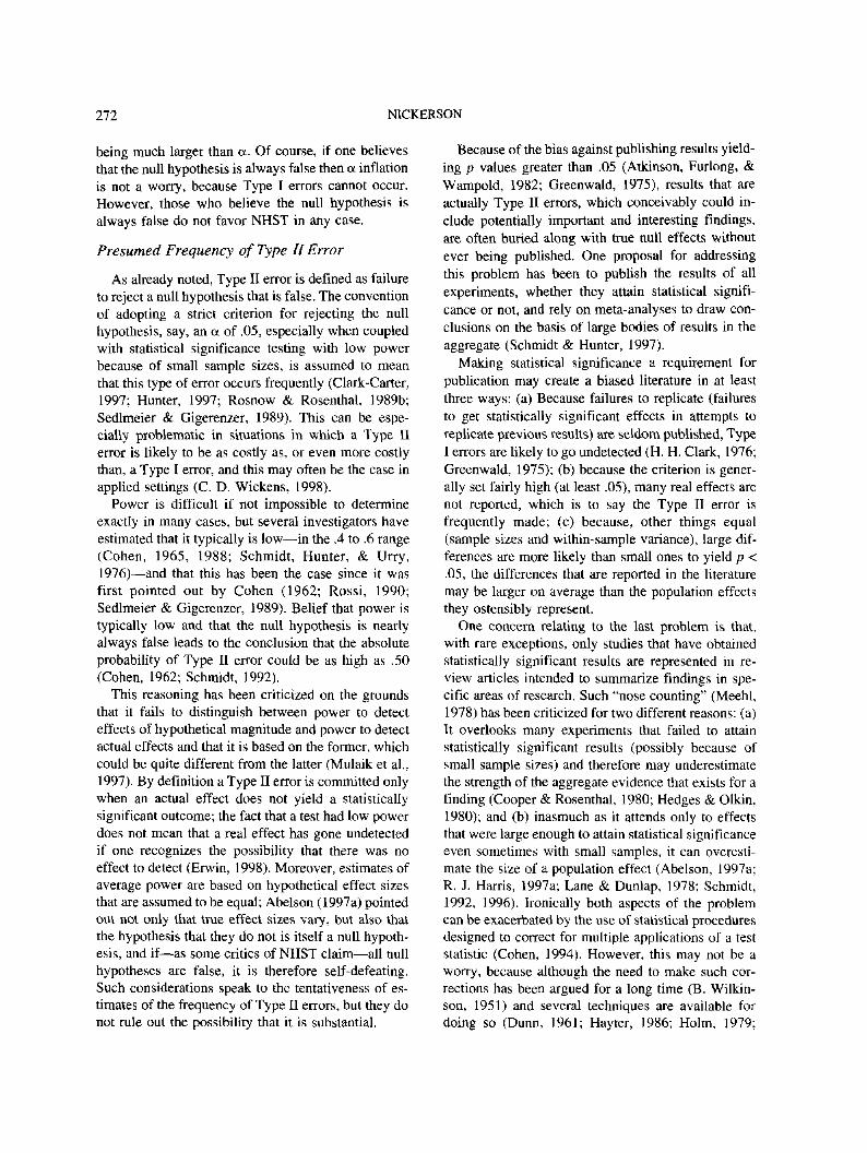
272 NICKERSON
being much larger than a. Of course, if one believes
that the null hypothesis is always false then a inflation
is not a worry, because Type I errors cannot occur.
However, those who believe the null hypothesis is
always false do not favor NHST in any case.
Presumed Frequency of Type H Error
As already noted, Type II error is defined as failure
to reject a null hypothesis that is false. The convention
of adopting a strict criterion for rejecting the null
hypothesis, say, an a of .05, especially when coupled
with statistical significance testing with low power
because of small sample sizes, is assumed to mean
that this type of error occurs frequently (Clark-Carter,
1997; Hunter, 1997; Rosnow & Rosenthal, 1989b;
Sedlmeier & Gigerenzer, 1989). This can be espe-
cially problematic in situations in which a Type II
error is likely to be as costly as, or even more costly
than, a Type I error, and this may often be the case in
applied settings (C. D. Wickens, 1998).
Power is difficult if not impossible to determine
exactly in many cases, but several investigators have
estimated that it typically is low—in the .4 to .6 range
(Cohen, 1965, 1988; Schmidt, Hunter, & Urry,
1976)—and that this has been the case since it was
first pointed out by Cohen (1962; Rossi, 1990;
Sedlmeier & Gigerenzer, 1989). Belief that power is
typically low and that the null hypothesis is nearly
always false leads to the conclusion that the absolute
probability of Type II error could be as high as .50
(Cohen, 1962; Schmidt, 1992).
This reasoning has been criticized on the grounds
that it fails to distinguish between power to detect
effects of hypothetical magnitude and power to detect
actual effects and that it is based on the former, which
could be quite different from the latter (Mulaik et al.,
1997). By definition a Type II error is committed only
when an actual effect does not yield a statistically
significant outcome; the fact that a test had low power
does not mean that a real effect has gone undetected
if one recognizes the possibility that there was no
effect to detect (Erwin, 1998). Moreover, estimates of
average power are based on hypothetical effect sizes
that are assumed to be equal; Abelson (1997a) pointed
out not only that true effect sizes vary, but also that
the hypothesis that they do not is itself a null hypoth-
esis, and if—as some critics of NHST claim—all null
hypotheses are false, it is therefore self-defeating.
Such considerations speak to the tentativeness of es-
timates of the frequency of Type II errors, but they do
not rule out the possibility that it is substantial.
Because of the bias against publishing results yield-
ing p values greater than .05 (Atkinson, Furlong, &
Wampold, 1982; Greenwald, 1975), results that are
actually Type II errors, which conceivably could in-
clude potentially important and interesting findings,
are often buried along with true null effects without
ever being published. One proposal for addressing
this problem has been to publish the results of all
experiments, whether they attain statistical signifi-
cance or not, and rely on meta-analyses to draw con-
clusions on the basis of large bodies of results in the
aggregate (Schmidt & Hunter, 1997).
Making statistical significance a requirement for
publication may create a biased literature in at least
three ways: (a) Because failures to replicate (failures
to get statistically significant effects in attempts to
replicate previous results) are seldom published, Type
I errors are likely to go undetected (H. H. Clark, 1976;
Greenwald, 1975); (b) because the criterion is gener-
ally set fairly high (at least .05), many real effects are
not reported, which is to say the Type II error is
frequently made; (c) because, other things equal
(sample sizes and within-sample variance), large dif-
ferences are more likely than small ones to yield p <
.05, the differences that are reported in the literature
may be larger on average than the population effects
they ostensibly represent.
One concern relating to the last problem is that,
with rare exceptions, only studies that have obtained
statistically significant results are represented in re-
view articles intended to summarize findings in spe-
cific areas of research. Such "nose counting" (Meehl,
1978) has been criticized for two different reasons: (a)
It overlooks many experiments that failed to attain
statistically significant results (possibly because of
small sample sizes) and therefore may underestimate
the strength of the aggregate evidence that exists for a
finding (Cooper & Rosenthal, 1980; Hedges & Olkin,
1980); and (b) inasmuch as it attends only to effects
that were large enough to attain statistical significance
even sometimes with small samples, it can overesti-
mate the size of a population effect (Abelson, 1997a;
R. J. Harris, 1997a; Lane & Dunlap, 1978; Schmidt,
1992, 1996). Ironically both aspects of the problem
can be exacerbated by the use of statistical procedures
designed to correct for multiple applications of a test
statistic (Cohen, 1994). However, this may not be a
worry, because although the need to make such cor-
rections has been argued for a long time (B. Wilkin-
son, 1951) and several techniques are available for
doing so (Dunn, 1961; Hayter, 1986; Holm, 1979;
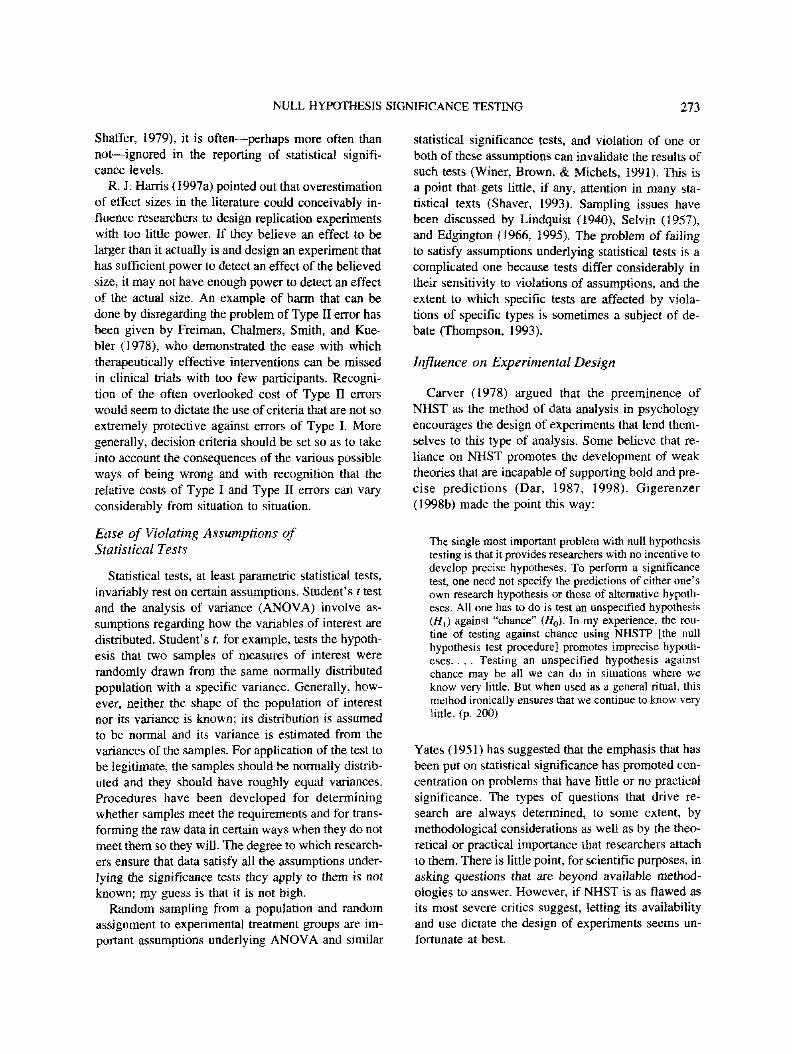
NULL HYPOTHESIS SIGNIFICANCE TESTING 273
Shaffer, 1979), it is often—perhaps more often than
not—ignored in the reporting of statistical signifi-
cance levels.
R. J. Harris (1997a) pointed out that overestimation
of effect sizes in the literature could conceivably in-
fluence researchers to design replication experiments
with too little power. If they believe an effect to be
larger than it actually is and design an experiment that
has sufficient power to detect an effect of the believed
size, it may not have enough power to detect an effect
of the actual size. An example of harm that can be
done by disregarding the problem of Type II error has
been given by Freiman, Chalmers, Smith, and Kue-
bler (1978), who demonstrated the ease with which
therapeutically effective interventions can be missed
in clinical trials with too few participants. Recogni-
tion of the often overlooked cost of Type D errors
would seem to dictate the use of criteria that are not so
extremely protective against errors of Type I. More
generally, decision criteria should be set so as to take
into account the consequences of the various possible
ways of being wrong and with recognition that the
relative costs of Type I and Type II errors can vary
considerably from situation to situation.
Ease of Violating Assumptions of
Statistical Tests
Statistical tests, at least parametric statistical tests,
invariably rest on certain assumptions. Student's t test
and the analysis of variance (ANOVA) involve as-
sumptions regarding how the variables of interest are
distributed. Student's t, for example, tests the hypoth-
esis that two samples of measures of interest were
randomly drawn from the same normally distributed
population with a specific variance. Generally, how-
ever, neither the shape of the population of interest
nor its variance is known; its distribution is assumed
to be normal and its variance is estimated from the
variances of the samples. For application of the test to
be legitimate, the samples should be normally distrib-
uted and they should have roughly equal variances.
Procedures have been developed for determining
whether samples meet the requirements and for trans-
forming the raw data in certain ways when they do not
meet them so they will. The degree to which research-
ers ensure that data satisfy all the assumptions under-
lying the significance tests they apply to them is not
known; my guess is that it is not high.
Random sampling from a population and random
assignment to experimental treatment groups are im-
portant assumptions underlying ANOVA and similar
statistical significance tests, and violation of one or
both of these assumptions can invalidate the results of
such tests (Winer, Brown, & Michels, 1991). This is
a point that gets little, if any, attention in many sta-
tistical texts (Shaver, 1993). Sampling issues have
been discussed by Lindquist (1940), Selvin (1957),
and Edgington (1966, 1995). The problem of failing
to satisfy assumptions underlying statistical tests is a
complicated one because tests differ considerably in
their sensitivity to violations of assumptions, and the
extent to which specific tests are affected by viola-
tions of specific types is sometimes a subject of de-
bate (Thompson, 1993).
Influence on Experimental Design
Carver (1978) argued that the preeminence of
NHST as the method of data analysis in psychology
encourages the design of experiments that lend them-
selves to this type of analysis. Some believe that re-
liance on NHST promotes the development of weak
theories thai are incapable of supporting bold and pre-
cise predictions (Dar, 1987, 1998). Gigerenzer
(1998b) made the point this way:
The single roost important problem with null hypothesistesting is that it provides researchers with no incentive todevelop precise hypotheses. To perform a significancetest, one need not specify the predictions of either one'sown research hypothesis or those of alternative hypoth-eses. All one has to do is test an unspecified hypothesis(H,) against "chance" (H0). In my experience, the rou-tine of testing against chance using NHSTP [the nullhypothesis test procedure] promotes imprecise hypoth-eses. . . . Testing an unspecified hypothesis againstchance may be all we can do in situations where weknow very little. But when used as a general ritual, thismethod ironically ensures that we continue to know verylittle, (p. 200)
Yates (1951) has suggested that the emphasis that has
been put on statistical significance has promoted con-
centration on problems that have little or no practical
significance. The types of questions that drive re-
search are always determined, to some extent, by
methodological considerations as well as by the theo-
retical or practical importance that researchers attach
to them. There is little point, for scientific purposes, in
asking questions that are beyond available method-
ologies to answer. However, if NHST is as flawed as
its most severe critics suggest, letting its availability
and use dictate the design of experiments seems un-
fortunate at best.
274 N1CKERSON
Defenses of NHST and RecommendationsRegarding Its Use
The abundance of criticisms notwithstanding,
NHST is not without its defenders (Baril & Cannon,
1995; Chow, 1987, 1988, 1989, 1991, 1996, 1998a,
1998b; Cortina & Dunlap, 1997; Cox, 1977; Dixon,
1998; Frick, 1996; Giere, 1972; R. J. Harris, 1997a,
1997b; Kalbfleisch & Sprott, 1976; Mulaik et al.,
1997; Robinson & Levin, 1997; Sohn, 1998b; W.
Wilson et al., 1967; Winch & Campbell, 1969). Pro-
ponents of NHST generally acknowledge that it has
limitations, and few if any argue that it should be the
only analytic tool in the researcher's repertoire. Some
point out that many of the criticisms of NHST are not
so much criticisms of NHST per se but criticisms of
some of its users and misuses. It is not the fault of the
process, they contend, if some of its users misunder-
stand it, expect more from it than it promises to de-
liver, or apply it inappropriately.
Abelson (1995, 1997a, 1997b) has defended NHST
when used judiciously, not as an unequivocal deter-
minant of what is worth reporting but as a means of
helping to justify claims that specific effects were
unlikely to have been obtained by chance. He argued
that the noteworthiness of an experimental finding is
determined by a variety of criteria, including the mag-
nitude, generality, and interestingness of the effect.
All statistics, in his view, should be treated as aids to
principled argument. He saw NHST as not the only,
but an essential, tool in the researcher's kit: "Signifi-
cance tests fill an important need in answering some
key questions, and if they did not exist they would
have to be invented" (1997b, p. 117). Dixon (1998)
contended that despite justified claims of the limita-
tions of NHST and misinterpretations of test results, p
values can convey useful information regarding the
strength of evidence: "Although p values are not the
most direct index of this information, they provide a
reasonable surrogate within the constraints posed by
the mechanics of traditional hypothesis testing" (p.
391).
Macdonald (1997) described both the Fisherian and
Neyman-Pearson approaches to statistical inference
as being "concerned with establishing that an ob-
served effect could not plausibly be accounted for by
sampling error" (p. 334). When an achieved signifi-
cance level—the probability of obtaining an effect as
extreme as the one observed—is sufficiently low, me
hypothesis that the obtained effect could plausibly be
due to sampling error is rejected, and rejection of this
hypothesis entails also rejection of the hypothesis of a
true effect opposite in direction to that observed. Mac-
donald defended the Fisherian approach but con-
tended that acquired significance levels should be
seen as a guide to whether an effect has been dem-
onstrated and not taken as the sole criterion.
Frick (1996) suggested that NHST is ideal for sup-
porting ordinal claims but not for evaluating models
that make quantitative predictions. By an ordinal
claim, he meant a claim that does not specify the size
of an effect but that specifies "only the order of con-
ditions, the order of effects, or the direction of a cor-
relation" (p. 380). Tukey (1991) contended that it is
really the direction of an effect rather than the exis-
tence of one that the t test helps decide. Others have
argued that if the question of interest is whether a
difference is positive or negative, NHST is a suitable
approach to finding out (Abelson, 1997b; R. J. Harris,
1997a, 1997b; W. Wilson et al., 1967).
Chow (1987,1988, 1989,1991,1996) has defended
NHST as a means of evaluating hypotheses, which he
noted are usually expressed in the form of an ordinal
relation such as a statement that performance is better
(or worse) under an experimental condition than un-
der a control condition. He made a distinction, how-
ever, between the problem of testing a hypothesis and
that of evaluating a theory. In his view, statistical
significance is relevant to hypothesis testing, but
theory evaluation requires integration of the results of
tests of many hypotheses that are deducible from the
theory in question and of other relevant information as
well. Hypothesis testing appropriately ends in a bi-
nary decision as to whether the data in hand are con-
sistent with the hypothesis or not; a theory is corrobo-
rated incrementally by the accumulation of evidence
from converging operations designed to test a variety
of hypotheses that are deducible from it. Chow (1989)
distinguished too, between the support a theory re-
ceives from a particular experiment and the theory's
overall status, the latter being determined "by how
often it has withstood attempts to falsify it, how well
it fares when compared to contending theories, how
extensive the converging operations in its support are"
(p. 164).
In his defense of NHST, Chow (1996, 1998a,
1998b) distinguished hypotheses at several levels of
abstraction—from lowest to highest: statistical, ex-
perimental, research, and substantive—and argued
that some of the criticisms that have been leveled at
NHST are based on failure to recognize the difference
between statistical hypotheses and higher level hy-
potheses. Other criticisms of NHST, he contended,
NULL HYPOTHESIS SIGNIFICANCE TESTING 275
are not appropriately aimed at NHST per se but at
inferential processes that are outside the domain of
statistics. It is especially important to recognize,
Chow (1998b) argued, that testing a statistical hypoth-
esis is not tantamount to testing a substantive (ex-
planatory, theoretical) hypothesis. Corroboration
(refutation) of a substantive hypothesis involves
showing that evidence (e.g., experimental data) is
consistent (inconsistent) with that hypothesis; show-
ing that a statistical hypothesis is or is not tenable can
be a factor in that process, but only one among many.
The limited but essential role of NHST, in Chow's
view, is that of ruling out chance (at a specified level
of strictness) as an explanation of data:
A significant result indicates a discernible effect in thesense that chance influences are excluded with referenceto a well-defined criterion. By the same token a signifi-cant effect is a genuine effect in the sense that it is notbrought about by chance factors. NHSTP is the indis-pensable tool for assessing whether or not chance influ-ences can be excluded as an explanation of the data.(1998b, pp. 327-329)
The claim that the role of NHST is to rule out
chance as an explanation of data is easily interpreted
as supportive of the belief that p represents the prob-
ability that chance is the operative factor given the
data, p(H0 I D); and we have already seen that this
belief is false, although p can be a reasonable proxy
for p(HQ I D) given certain assumptions that appear to
often be plausible. Furthermore, psychologists use
NHST to test substantive hypotheses in theory-
corroborating studies whether or not it is adequate to
that task. Dar (1998) spoke to the latter point this way:
"The move from the substance to the statistical hy-
pothesis is a swift one: researchers interpret statistical
significance as confirming the substantive hypothesis
and therefore as corroborating the theory from which
the hypothesis was derived" (p. 196). This, of course,
is a criticism of the behavior of researchers and not of
NHST per se.
In an attempt to account for the popularity of
NHST, Greenwald et al. (1996) argued that it provides
a dichotomous outcome that can be used for decision
making, that/7 is a common-language translation for a
variety of statistics (having one measure of how sur-
prising a result should be under the hypothesis of no
effect makes it unnecessary to deal with many such
indicants), and that p also constitutes a measure of
confidence in the replicability of null hypothesis re-
jection. (As noted in the foregoing, the question of
whether p is a justified measure of confidence in rep-
licability is a contested one.) These are all desirable
properties in the eyes of NHST users.
Mulaik et al. (1997) argued that much of the oppo-
sition to NHST stems from confusion on a variety of
subjects. They noted several beliefs, including some
of those mentioned in the first part of this article, all
of which they considered to be incorrect. They con-
tended that many of the criticisms of NHST really
pertain to misconstruals or misuses of significance
tests and thus may speak to the incompetence of the
misusers, but do not demonstrate the invalidity of the
approach per se. Criticisms of "abusive misconcep-
tions of the use and interpretation of significance test-
ing," Mulaik et al. insisted, "can hardly be regarded as
criticisms of significance testing properly understood
and applied" (p. 74). The fact that there are arsonists
in the world does not make fire a bad thing. A similar
position has been taken by Rossi (1997).
A common misuse of significance tests is to con-
clude that a difference due to two treatments, A and B,
is statistically significant on the grounds that the ef-
fect of A is significantly different from zero and that
of B is not. Regarding whether this type of confusion
should be held against the test per se, Abelson
(1997b) had this comment: "If a legal case were being
brought against the significance test, the charge here
would be that the test is an 'attractive nuisance,' like
a neighbor's pond in which children drown. It tempts
you into making inappropriate statements" (p. 120).
As for the contention that NHST should be banned,
Mulaik et al. (1997) took the opposite position:
We cannot get rid of significance tests because theyprovide us with the criteria by which provisionally todistinguish results due to chance variation from resultsthat represent systematic effects in data available to us.As long as we have a conception of how variation inresults may be due to chance and regard it as applicableto our experience, we will have a need for significancetests in some form or another, (p. 81)
Calls for the banning of NHST, Mulaik et al. argued,
stem from a conception of NHST that overlooks the
provisional nature of conclusions that result from it.
In addition to defending the use of NHST, propo-
nents of it have offered several suggestions regarding
how it might be use more effectively. I turn next to a
consideration of some of these suggestions.
Make Greater Use of Non-Nil Null Hypotheses
Some of the problems associated with NHST dis-
appear or at least diminish if the null hypothesis is
276 NICKERSON
defined as something other than a hypothesis of zero
difference, zero effect, or zero correlation (the nil null
hypothesis). Ideally one would like to be able to make
precise quantitative predictions of the effects of ex-
perimental manipulations, but most areas of psychol-
ogy do not permit a high degree of precision at their
present level of development. It does not follow that
one must settle for the nil null hypothesis in all cases,
however. Quasiquantitative predictions, of rough
magnitudes of effects, could help advance the field
(Blaich, 1998).
Mulaik et al. (1997) distinguished between the
problem of deciding what hypothesis one should test
and that of applying NHST procedures appropriately
to whatever that hypothesis is. The same writers sug-
gested that one way to facilitate knowledge accumu-
lation in psychology is to use what is learned in ex-
periments to establish values for non-nil null
hypotheses in subsequent experiments: "A hypothesis
one ought to test is that the effect is equal to the value
estimated in the previous study, which one judged to
be significantly different from a zero effect" (p. 98).
This possibility has also been pointed out by Green-
wald et al. (1996). Mulaik et al. noted that with ex-
isting ANOVA methods and programs it is not easy to
specify hypotheses in terms of previously found ef-
fects, and they suggested the desirability of some
modernization of ANOVA in this regard. Some will
see this suggestion as an argument for applying a
Bayesian approach to data analysis.
Use Range Null Hypotheses
An alternative to the use of the point null hypoth-
esis that has been urged by several writers is the use
of a range null hypothesis, which involves designating
a range of values that will be considered effectively
null (Hodges & Lehmann, 1954; Meehl, 1967; Serlin,
1993; Serlin & Lapsley, 1985, 1993; Yeaton &
Sechrest, 1986). Serlin (1993) argued that how wide
the range should be depends on the state of the theory
of interest but that, in any case, it should be specified
in advance of an experiment. Some writers have taken
the position that when testing a point null hypothesis
researchers typically mean to treat it as a proxy for a
range hypothesis anyway, which is to say that they
usually do not seriously consider a difference of ex-
actly zero to be probable, but they use zero to repre-
sent anything close (without specifying how close) to
it. Cortina and Dunlap (1997) surmised that although
it would be better if researchers specified the range of
values they would consider within the "good-enough
belt" described by Serlin and Lapsley (1985), "the
vast majority of research that has focused on the nil
would have been very much the same even if an al-
ternative null value had been used" (p. 167).
Be Specific About the Alternative(s) to theNull Hypothesis
The predominant NHST paradigm leaves the alter-
native to the null hypothesis unspecified beyond "dif-
ferent from zero," or in the case of one-tailed tests,
"less (greater) than zero." It is possible, however, to
have a specific alternative to a null hypothesis, which
can be composite with as many independent compo-
nents as one likes. Expression of a specific alternative
hypothesis moves one in the direction of using Bayes-
ian statistics, and some researchers object to this on
the grounds that it usually requires the introduction of
subjectivism because of the need to assign prior prob-
abilities to the hypotheses and a probability to the data
conditional on the alternative hypothesis. A counter to
this argument is that subjective judgment is required
in conventional non-Bayesian hypothesis testing as
well, but in this case it is not quite so apparent.
I. J. Good (1981/1983b), who sees himself as nei-
ther a Bayesian nor an anti-Bayesian, argued this way
for making the alternative hypothesis precise and ex-
plicit:
I believe it is a feature of all sensible significance-testcriteria that they are chosen with either a precise or,more often, a vague non-null hypothesis, in mind. In thisrespect "non-Bayesians" act somewhat like Bayesians. //a tail-area probability is small enough then it is worthwhile to try to make the non-null hypothesis less vagueor even to make it precise, and the smaller the tail-areaprobability, the more worth while it is to make this at-tempt. . . . It is sometimes stated by Fisherians that theonly hypothesis under consideration is the null hypoth-esis, but I am convinced that this is only a way of sayingthat the non-null hypothesis is vague, not that it does notexist at all. (pp. 138-140)
A similar point has been made by Rogers et al.
(1993), who argued that it is not a small p value alone
that determines a researcher's postexperiment belief
about the null hypothesis, but "a small p value with a
known experimental manipulation after random as-
signment" (p. 560) that does so. As a rule (though not
always), an experimenter has a definite idea of how a
planned manipulation will affect the dependent vari-
able(s) of interest, at least to the extent of the direction
of the anticipated effect. Rogers et al.'s point is that
this idea, along with the value of p, determines the
NULL HYPOTHESIS SIGNIFICANCE TESTING 277
experimenter's interpretation of the outcome, which
from a Bayesian point of view is as it should be.
The overarching issue here is that what constitutes
appropriate statistical treatment of the data obtained in
an experiment and justified interpretation of the out-
come depends to no small degree on the experiment-
er's preexperiment intentions and expectations. For
this reason, experimenters should make explicit their
preexisting expectations—alternative hypothesis(es)
and its (their) predictions regarding data. This is not to
suggest that unexpected patterns in data cannot be
informative and should be ignored. However, what
they provide are generally better viewed as clues to
possible relationships that should be explored in fur-
ther experimentation, not statistical justification for
firm conclusions that such relationships exist.
Report p Values
Several writers, including Fisher (1956/1990), have
advocated the reporting of actual p values as an alter-
native or complement to classifying results as either
significant or not significant relative to a given a
criterion (Abelson, 1995; Eysenck, 1960; Gibbons &
Pratt, 1975; I. J. Good, 1981/1983b; Greenwald et al.,
1996; Huberty, 1993; Schafer, 1993; Upton, 1992;
Wang, 1993). Especially bothersome is the practice of
reporting only whether the outcomes of tests attained
statistical significance and not giving the values of the
test statistics or, in some cases, means and standard
deviations on which they were based (Meehl, 1978,
1997).
The reporting of p values makes the reporting of
results a more objective process: When an investiga-
tor reports thatp = .045 in one case andp = .055 in
another, the reader can decide whether to consider one
significant and the other not. On the other hand, re-
porting p values is not necessarily inconsistent with
using an ce criterion. There is the view that p values
should be reported so readers can draw their own
conclusions but that the conclusions drawn by experi-
menters should be based on their predetermined cri-
teria; Cortina and Dunlap (1997) expressed this view
and argued that the latter restriction follows from the
logic of theory testing, which involves determining
whether predicted results are obtained.
Another argument for reporting actual p values is
that it facilitates the aggregation of evidence across
experiments by the use of meta-analyses. The practice
is simplified by the fact that widely used statistical
software packages yield specific values of p.
A minor problem associated with reporting actual p
values is the fact that some software data-analysis
packages return such values as .0000. Presumably this
means that p = 0 to four decimal places; however,
many readers object to the representation. A compro-
mise is to revert to p < .0001 for all values of p less
than .0001.
Summary of Defenses of NHST andRecommendations Regarding Its Use
Several writers have defended the use of NHST as
an aid to the interpretation of experimental results and
have argued that most if not all of the criticisms of it
are more appropriately directed at ways in which it is
sometimes misapplied and are not justified criticisms
of NHST per se. Some defenders of NHST acknowl-
edge that many users have misconceptions of it and
consequently misapply it, but they argue that many of
the criticisms that are leveled against the procedure
are based on misconceptions or false beliefs as well.
Proponents of the use of NHST have also suggested
several ways in which the effectiveness of its use
might be enhanced. These suggestions include mak-
ing greater use of non-nil null hypotheses, including
range null hypotheses; being specific about alterna-
tives to the null hypothesis; and reporting of actual p
values rather than only classifying outcomes as either
statistically significant or not statistically significant
relative to a prespecified criterion.
Alternatives or Supplements to NHST
As noted early in this article, some of the NHST's
critics argue that this method of data analysis should
be abandoned. Nobody, to my knowledge, even
among its staunches! defenders has argued that NHST
is the only type of analysis of data that one needs to
do. In what follows, I note a variety of suggestions
that have been made of ways either to supplement
NHST or to replace it with alternative methods for
evaluating the results of research.
Provide Some Indication of Variability orPrecision of Measurement
Although variability due to measurement error is
widely recognized as an important consideration in
the evaluation of data obtained in nearly all psycho-
logical experiments, indications of it are lacking in
many published reports of experimental results, and
especially on the figures appearing in those reports.
Estes (1997a) argued strongly for the inclusion of
indications of variability on graphical representations
278 NICKERSON
of data but cautioned that such indications should be
accompanied by information regarding what data they
are based on and how they were computed.
Some measures of variability (e.g., standard devia-
tions, interquartile ranges) are simply descriptive of
the data in hand and say nothing directly regarding the
populations from which samples have been drawn.
Others (e.g., standard errors of means and confidence
intervals) are used to make inferences about the vari-
ability of populations and are subject to misconcep-
tions and confusions not unlike those that pertain to
the p values of NHST.
The standard error of the mean is an estimator of
the standard deviation of sample means around a
population mean, and when used to bracket the popu-
lation mean it indicates the range around the true
mean within which about two thirds of the means of
replicated random samples would be expected to fall.
In actual experiments (simulations aside) population
means are not known and standard error bars are usu-
ally drawn around sample means, and here they invite
misinterpretation. They do not indicate the range
around a sample mean within which about two thirds
of the means of replicated random samples would fall.
Given reasonable assumptions about the relationship
between the standard error of the mean and the stan-
dard deviation of the population of sample means,
about two thirds of the means of replicated random
samples would fall within a range of about 1.4 times
the standard error on either side of the sample mean
(Estes, 1997a). Estes explained the common misinter-
pretation of standard errors and gave guidelines for
computing and communicating measures of variabil-
ity based on sample data for both independent-group
and repeated-measures experimental designs.
Report Confidence Intervals Around
Point Estimates
Among the indications of variability that might be
used, confidence intervals deserve special attention
because the reporting of them around point estimates
has been advocated as an alternative, or adjunct, to
NHST by many writers, including both critics and
proponents of NHST (Bailer & Hosteller, 1988;
Bolles & Messick, 1958; Cohen, 1990, 1994; Gardner
& Altaian, 1986; Gonzalez, 1994; Grant, 1962;
Hunter, 1997; Jones, 1995; Loftus, 1991; Loftus &
Masson, 1994; Meehl, 1997; Mulaik et al., 1997; Ro-
zeboom, 1960; Schmidt, 1996; Serlin, 1993; Steiger
& Fouladi, 1997; Tukey, 1991).
Although confidence intervals are probably most
commonly reported for means or for differences be-
tween means, they can be computed for other statis-
tics as well. Usually upper and lower interval bounds
are equidistant from the estimated point value, but
they are not always so (Darlington & Carlson, 1987).
Steiger and Fouladi (1997) made a strong case for the
advantages of confidence intervals and described a
general method for computing them for variables for
which they are seldom reported. Techniques for com-
puting confidence intervals around means for be-
tween-subjects experimental designs are readily avail-
able; recently Loftus and Masson (1994) have
described procedures for computing such intervals for
within-subject designs. The fact that these cases re-
quire different computations suggests the need for
care in reporting computational approaches along
with the intervals computed (Estes, 1997a).
An attraction that is claimed for point estimates
bracketed with confidence intervals is that confidence
intervals are more informative than significance tests.
One gets both an estimate of effect size and an indi-
cation of uncertainty as to its accuracy. These esti-
mates can be especially helpful when there is interest
in showing that the effect of some experimental treat-
ment is nonexistent or small (e.g., an unwanted side
effect of a new drug). Reichardt and Gollob (1997)
suggested that attaching more importance to precision
of estimates (e.g., narrowness of confidence intervals)
in publication decisions could help address problems
stemming from the overriding importance now at-
tached to statistical significance. Hedges (1987) ar-
gued that something equivalent to the determination
of confidence intervals is typically done in the physi-
cal sciences. (See also Meehl, 1967, in this regard.)
Mulaik et al. (1997) noted that one reason that physi-
cal scientists do not use NHST so much is that they
are not always testing hypotheses but rather trying to
improve estimates of physical constants.
Some writers have cautioned that although confi-
dence intervals can be very effective aids to the in-
terpretation of data, they are subject to the some of the
same types of misconceptions and misuses as is
NHST (Abelson, 1997a; Cortina & Dunlap, 1997;
Frick, 1995b, 1996; Hayes, 1998). As Abelson
(1997a) said: "Under the Law of Diffusion of Idiocy,
every foolish application of significance testing will
beget a corresponding foolish practice for confidence
limits" (p. 13). Steiger and Fouladi (1997) warned that
the proper use of confidence intervals requires as-
sumptions about distributions, just as NHST does, and
NULL HYPOTHESIS SIGNIFICANCE TESTING 279
that if the assumptions are not met the resulting in-
tervals can be inaccurate. In particular, they noted that
"the width of a confidence interval is generally a ran-
dom variable, subject to sampling fluctuations of its
own, and may be too unreliable at small sample sizes
to be useful for some purposes" (p. 254). Cortina and
Dunlap (1997) argued that simply replacing NHST
with the use of confidence intervals could create the
illusion that all the problems associated with NHST
have thereby been solved when many of them may not
even have been addressed.
Essential to an understanding of confidence inter-
vals is the distinction between an interval around a
population parameter and one around a sample statis-
tic. These do not have the same meaning (Estes,
1997a). The theory underlying the use of confidence
intervals is based on repeated random sampling from
a known population and supports conclusions about
confidence intervals drawn around that population's
parameters. However, with rare exceptions, popula-
tion parameters are not known in empirical research—
the point of the research generally is to provide a basis
for estimating them—and confidence intervals are
drawn around the sample statistics.
A common misinterpretation of a confidence inter-
val of x% around a statistic (e.g., sample mean) is that
the probability is x that the parameter of interest (e.g.,
population mean) lies within the interval, or more
operationally that it is the interval around the statistic
within which x% of measures of the same statistic on
additional samples drawn in the same way would fall.
It is easy to find discussions of confidence intervals
that convey just this idea, which would be true if the
first measure of the statistic happened to coincide with
the population parameter and all subsequent samples
were randomly drawn from the same population, but
not otherwise. This misinterpretation may be rein-
forced by language such as the following that is some-
times found in statistics texts: "An alternative ap-
proach to estimation is to extend the concept of error
bound to produce an interval of values that is likely to
contain the true value of the parameter" (Bhat-
tacharyya & Johnson, 1977, p. 243). The authors of
this comment went on to point out that it is not correct
to interpret a confidence interval of, say, 95% as an
indication that the probability that the parameter of
interest lies within the specified interval is .95, but it
would not be surprising if the above comment itself is
interpreted by readers in that way.
Another example comes from Elifson, Runyon, and
Haber (1990), who after computing upper and lower
limits for the 95% confidence interval for a sample
mean of 108 and sample standard deviation of 15 said,
Having established the lower and upper limits as 101.82and 114.18, respectively, we may now conclude: On thebasis of our obtained mean and standard deviation,which were computed from scores drawn from a popu-lation in which the true mean is unknown, we assert thatthe population mean probably falls within the intervalthat we have established, (p. 367)
These authors went on to caution, "Since the popula-
tion mean is a fixed value and does not have a distri-
bution, our probability statements never refer to u,." I
find it difficult to see these two assertions as consis-
tent.
Bhattacharyya and Johnson (1977) contended that
given an appropriately computed confidence interval
of x% it is correct to say that one is x% confident that
the parameter of interest lies within the interval, but it
is not correct to say that the probability is x that the
parameter lies within the interval. The statement of
confidence, in this view, rests on the expectation that
for 95% of the samples of the same size drawn at
random from the same population, confidence inter-
vals computed in the same way will contain the value
of the parameter, which is different from the belief
that the probability is .95 that the parameter lies
within the particular interval computed. (See also
Darlington & Carlson, 1987; Elifson et al., 1990;
Pruzek, 1997, regarding the same distinction.) This is
a subtle distinction, even discounting the thorny ques-
tion of what probability really means, and it is not
hard to understand that with respect to the interpreta-
tion of confidence intervals confusion appears to
reign.
Inasmuch as reporting confidence intervals has
been urged by many parties on both sides of the de-
bate about NHST, the infrequency of their appearance
in published articles (Kirk, 1996) begs an explanation.
The question is the more puzzling in view of the fact
that the use of point estimates and confidence inter-
vals ("error bands") predates the development of
NHST (Oakes, 1986; Schmidt & Hunter, 1997). Co-
hen's (1994) surmise is that the reason they are not
reported is that, at least when set at 95% to correspond
to a .05 a level, they typically are embarrassingly
large.
Reichardt and Gollob (1997) ventured several "po-
tential sources of resistance to the use of confidence
intervals" (p. 277), which in abbreviated form are as
follows: (a) convention (strength of tradition); (b) lack
280 NICKERSON
of recognition of conditions in which confidence in-
tervals are preferable to significance tests; (c) relative
paucity of computer programs and formulas for com-
puting confidence intervals; (d) the often disappoint-
ingly small size of parameter estimates—confidence
intervals reveal this whereas significance tests do not;
(e) the often disappointingly wide range of confidence
intervals; (f) the absence of unique confidence inter-
vals when no uniquely defined parameter is associated
with a statistical test, which means computing a con-
fidence interval may mean choosing among candidate
indexes and defending the choice; (g) arguments
against significance testing recognized to be falla-
cious that may, in some cases, damage the credibility
of claims of the superiority of confidence intervals;
and (h) some researchers' rejections of recommenda-
tions to abandon NHST (which sometimes accom-
pany promotion of the use of confidence intervals)
because they interpret them to be recommendations to
abandon hypothesis testing more generally and they
do not consider that to be desirable.
Estes (1997a) cautioned that because confidence
intervals can be computed in different ways, the
method of computation must be known in any par-
ticular case if confusion is to be avoided. (Methods of
computation depend on such considerations as sample
size, whether the standard deviation of the population
is known, whether the distribution of interest is sym-
metric, and so on.) He recommended against showing
"quasi" confidence intervals (intervals calculated
from interaction terms rather than from within-cell
mean squares) on figures, on the grounds that show-
ing them could invite misinterpretation. He noted, too,
the importance of consistently using intervals of the
same width (percentage) within a given research re-
port.
Report Effect Size
Many writers have recommended that researchers
standardly provide some indication of effect size ei-
ther along with or in place of the results of statistical
significance tests (Abelson, 1995; Carver, 1978,
1993; Cohen, 1988; Cook & Campbell, 1979; Fisher,
1925; Fleiss, 1969; Folger, 1989; Friedman, 1968;
Glass, 1976; Guttman, 1981; M. J. Harris, 1991; M. J.
Harris & Rosenthal, 1985; Hurlburt, 1994; Katzer &
Sodt, 1973; Loftus, 1993; Nelson et al., 1986; Scha-
fer, 1993; Schmidt, 1996; Snyder & Lawson, 1993;
Thompson, 1994a, 1996). The reporting of effect size
is required by some journal editors (Murphy, 1997;
Thompson, 1994a); it is encouraged but not required
by the Publication Manual of the American Psycho-
logical Association (4th ed., APA, 1994, p. 16).
The term effect size has an unfortunate ambiguity as
applied to the results of experimentation. Its most
straightforward connotation is that of the magnitude
of some measure, such as the size of the difference
between two means or the degree of association (co-
variation) between two variables. It can also suggest,
however, the theoretical or practical impact of a find-
ing. The former connotation is intended here and, I
believe, in most discussions of effect size in the psy-
chological literature, but the ambiguity is a source of
confusion. (Sometimes a distinction is made between
measures of effect size and measures of strength of
relationship [e.g., Kirk, 1996], but for present pur-
poses it will suffice to let the meaning of effect size be
sufficiently broad to encompass both.) As Maher
(1998) noted it is unfortunate that the word effect is
used to denote a computation "that tells us nothing
about the concrete effects produced by an interven-
tion" (p. 211). Shaver (1991, 1993), who argued for
another reason that the term should be result size,
contended that this should always be reported and that
the results of statistical significance tests and of power
analyses should never be.
A variety of indicants of effect size have been pro-
posed (Cliff. 1993; Cohen, 1962, 1977; Cohen & Co-
hen, 1983; Fleiss, 1969; Friedman, 1968; Hays, 1994;
Hedges, 1981; Judd, McClelland, & Culhane, 1995;
Maxwell, Camp, & Arvey, 1981; Rosenthal & Rubin,
1982; Snyder & Lawson, 1993; Tatsuoka, 1993). Sev-
eral, including the actual magnitude of the observed
effect (e.g., difference between means), a standard-
ized magnitude (the actual magnitude normalized by
the within-groups standard deviation), Pearson's r and
r2, and a measure of "causal efficacy" (the raw mag-
nitude of effect divided by the magnitude of the varia-
tion in the independent variable) are discussed by
Abelson (1995). The Publication Manual of the
American Psychological Association (4th ed.; APA,
1994) mentions as common measures "r2, T|2, to2, R2,
4>2, Cramer's V, Kendall's W, Cohen's d and K, Good-
man and Kruskal's \ and -y, Jacobson and Truax's
(1991) proposed measure of clinical significance, and
the multivariate Roy's 0 and the Pillai-Bartlett V" (p.
18). Kirk (1996) listed almost all of these plus several
others; however, on the basis of a survey of four APA
journals, he noted that most of these measures are
seldom if ever found in published reports.
Among the more widely used indicants is r2 (some-
times called the coefficient of determination), which
NULL HYPOTHESIS SIGNIFICANCE TESTING 281
shows the percentage of variance in a dependent vari-
able accounted for by variance in an independent vari-
able. Some writers have argued that r is a better in-
dicant than r2, however, for many practical purposes
(Nelson et al., 1986). Rosenthal and Rubin (1982)
believed that the importance of effects are often un-
derestimated when the value of r2 is small especially
perhaps in biomedical or clinical contexts.
Another widely used indicant of effect size is Co-
hen's (1962, 1988) d, which is the difference between
means divided by the pooled within-groups standard
deviation. Like the familiar z score, d expresses a
difference in standard-deviation units. Such a measure
has the advantage of facilitating comparisons of effect
sizes across studies involving measurements on dif-
ferent scales.
Pointing out that statistical significance is a func-
tion of two factors—effect size and sampling error—
Carver (1993) argued that reporting each of these
measures is preferable to reporting a statistic such as
t that combines them.
Statistical significance tells us nothing directly relevant
to whether the results we found are large or small, and it
tells us nothing with respect to whether the sampling
error is large or small. We can eliminate this problem by
reporting both effect size and standard errors, (p. 291)
The reporting of effect size, however, is not totally
free of problems. Which one of various possible ef-
fect-size estimates is most appropriate in a given con-
text is not always apparent (Rosenthal, 1991), and
opinions differ regarding the merits of specific possi-
bilities (Crow, 1991; Gorsuch, 1991; McGraw, 1991;
Parker, 1995; Rosenthal, 1991; Strahan, 1991). More-
over, the implications of effect-size estimates, like
those of other statistics, need to be interpreted care-
fully. It is not safe to assume, for example, that the
size of an effect obtained with one population, such as
college students, will generalize readily to other
populations, such as nonstudents (Sears, 1986).
Furthermore, a large effect is no more of a guaran-
tee of the theoretical or practical importance of a
finding than is a small p value resulting from a sig-
nificance test (Chow, 1991; Shaver, 1985); a small
effect may be very important in some contexts and a
large one of little interest in others (Lewandowsky &
Maybery, 1998; Prentice & Miller, 1992; Rosenthal,
1990; Rosenthal & Rubin, 1979). Finally, effect size
should not be confused with strength of belief; as
Abelson (1995) has pointed out, one may have a
strong belief in a small effect or a weak belief in a
large one.
The reporting of effect size may be seen as consis-
tent with the use of NHST and an important comple-
ment to it (Hagen, 1998; Thompson, 1993). Robinson
and Levin (1997) recommended the policy of first
determining whether an effect is statistically improb-
able and then, only if it is, including in the reporting
an indication of its size. Alternatively, as already
noted, one may decide first the minimum effect size
that would be large enough to be of interest and then
use NHST to test the hypothesis that the effect is
statistically significant only if it meets the size test
(Fowler, 1985).
Rosnow and Rosenthal (1989b) maintained mat ef-
fect sizes should be calculated whether or not/? values
reach conventional levels of statistical significance.
They noted that effect size tells the experimenter
something that a p value does not, and they suggested
that such computations can be useful in determining
sample sizes for subsequent experimentation. The
standard reporting of effect size has the added attrac-
tion for some analysts of facilitating the use of meta-
analytic techniques (Asher, 1993; Glass et al., 1981;
M. J. Harris & Rosenthal, 1985; Mullen, 1989; Rosen-
thai, 1984). Despite urgings for the consistent report-
ing of effect size, it appears not to have become stan-
dard practice yet (Kirk, 1996; Thompson & Snyder,
1997, 1998). One practical impediment to the use of
effect-size indicants as well as of confidence intervals
may be poor understanding of them among research-
ers (Svyantek & Ekeberg, 1995).
A contrary view regarding the importance of re-
porting effect sizes has been given by Chow (1988,
1996), who argued that it can be important when an
experimenter is interested in an experimental effect
per se and the purpose of an experiment is to deter-
mine whether that effect is of sufficient size to have
practical importance (utilitarian experiment), but that
it is not relevant when the purpose of the experiment
is to test an implication of an explanatory theory
(theory-corroboration experiment). In the latter case,
Chow (1996) claimed, the only relevant consideration
is whether the obtained result is consistent with that
predicted by the theory, within the criterion repre-
sented by the a level, and that an emphasis on effect
size in this context can be misleading. Chow (1996)
stressed that obtaining a result that is consistent in this
statistical sense with the implications of a theory does
not prove the theory true, but he argued that it does
add incrementally to the theory's tenability.
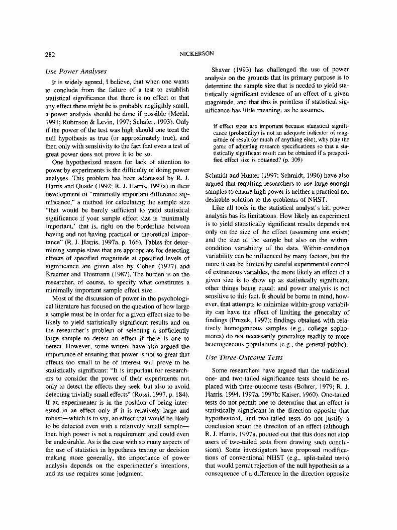
282 NICKERSON
Use Power Analyses
It is widely agreed, I believe, that when one wants
to conclude from the failure of a test to establish
statistical significance that there is no effect or that
any effect there might be is probably negligibly small,
a power analysis should be done if possible (Meehl,
1991; Robinson & Levin, 1997; Schafer, 1993). Only
if the power of the test was high should one treat the
null hypothesis as true (or approximately true), and
then only with sensitivity to the fact that even a test of
great power does not prove it to be so.
One hypothesized reason for lack of attention to
power by experiments is the difficulty of doing power
analyses. This problem has been addressed by R. J.
Harris and Quade (1992; R. J. Harris, 1997a) in their
development of "minimally important difference sig-
nificance," a method for calculating the sample size
"that would be barely sufficient to yield statistical
significance if your sample effect size is 'minimally
important,' that is, right on the borderline between
having and not having practical or theoretical impor-
tance" (R. J. Harris, 1997a, p. 166). Tables for deter-
mining sample sizes that are appropriate for detecting
effects of specified magnitude at specified levels of
significance are given also by Cohen (1977) and
Kraemer and Thiemann (1987). The burden is on the
researcher, of course, to specify what constitutes a
minimally important sample effect size.
Most of the discussion of power in the psychologi-
cal literature has focused on the question of how large
a sample must be in order for a given effect size to be
likely to yield statistically significant results and on
the researcher's problem of selecting a sufficiently
large sample to detect an effect if there is one to
detect. However, some writers have also argued the
importance of ensuring that power is not so great that
effects too small to be of interest will prove to be
statistically significant: "It is important for research-
ers to consider the power of their experiments not
only to detect the effects they seek, but also to avoid
detecting trivially small effects" (Rossi, 1997, p. 184).
If an experimenter is in the position of being inter-
ested in an effect only if it is relatively large and
robust—which is to say, an effect that would be likely
to be detected even with a relatively small sample—
then high power is not a requirement and could even
be undesirable. As is the case with so many aspects of
the use of statistics in hypothesis testing or decision
making more generally, the importance of power
analysis depends on the experimenter's intentions,
and its use requires some judgment.
Shaver (1993) has challenged the use of power
analysis on the grounds that its primary purpose is to
determine the sample size that is needed to yield sta-
tistically significant evidence of an effect of a given
magnitude, and that this is pointless if statistical sig-
nificance has little meaning, as he assumes.
If effect sizes are important because statistical signifi-cance (probability) is not an adequate indicator of mag-nitude of result (or much of anything else), why play thegame of adjusting research specifications so that a sta-tistically significant result can be obtained if a prespeci-fied effect size is obtained? (p. 309)
Schmidt and Hunter (1997; Schmidt, 1996) have also
argued that requiring researchers to use large enough
samples to ensure high power is neither a practical nor
desirable solution to the problems of NHST.
Like all tools in the statistical analyst's kit, power
analysis has its limitations. How likely an experiment
is to yield statistically significant results depends not
only on the size of the effect (assuming one exists)
and the size of the sample but also on the within-
condition variability of the data. Within-condition
variability can be influenced by many factors, but the
more it can be limited by careful experimental control
of extraneous variables, the more likely an effect of a
given size is to show up as statistically significant,
other things being equal; and power analysis is not
sensitive to this fact. It should be borne in mind, how-
ever, that attempts to minimize within-group variabil-
ity can have the effect of limiting the generality of
findings (Prazek, 1997); findings obtained with rela-
tively homogeneous samples (e.g., college sopho-
mores) do not necessarily generalize readily to more
heterogeneous populations (e.g., the general public).
Use Three-Outcome Tests
Some researchers have argued that the traditional
one- and two-tailed significance tests should be re-
placed with three-outcome tests (Bohrer, 1979; R. J.
Harris, 1994, 1997a, 1997b; Kaiser, 1960). One-tailed
tests do not permit one to determine that an effect is
statistically significant in the direction opposite that
hypothesized, and two-tailed tests do not justify a
conclusion about the direction of an effect (although
R. J. Harris, 1997a, pointed out that this does not stop
users of two-tailed tests from drawing such conclu-
sions). Some investigators have proposed modifica-
tions of conventional NHST (e.g., split-tailed tests)
that would permit rejection of the null hypothesis as a
consequence of a difference in the direction opposite
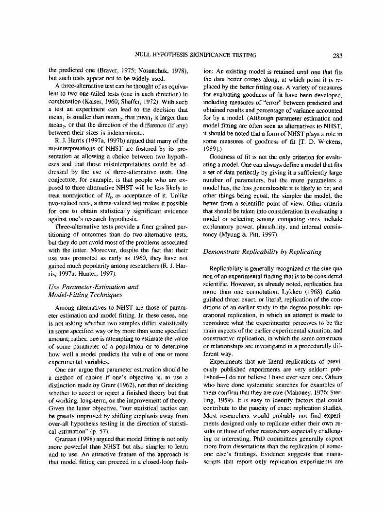
NULL HYPOTHESIS SIGNIFICANCE TESTING 283
the predicted one (Braver, 1975; Nosanchuk, 1978),
but such tests appear not to be widely used.
A three-alternative test can be thought of as equiva-
lent to two one-tailed tests (one in each direction) in
combination (Kaiser, 1960; Shaffer, 1972). With such
a test an experiment can lead to the decision that
mean, is smaller than mean2, that mean, is larger than
mean2, or that the direction of the difference (if any)
between their sizes is indeterminate.
R. J. Harris (1997a, 1997b) argued that many of the
misinterpretations of NHST are fostered by its pre-
sentation as allowing a choice between two hypoth-
eses and that those misinterpretations could be ad-
dressed by the use of three-alternative tests. One
conjecture, for example, is that people who are ex-
posed to three-alternative NHST will be less likely to
treat nonrejection of H0 as acceptance of it. Unlike
two-valued tests, a three-valued test makes it possible
for one to obtain statistically significant evidence
against one's research hypothesis.
Three-alternative tests provide a finer grained par-
titioning of outcomes than do two-alternative tests,
but they do not avoid most of the problems associated
with the latter. Moreover, despite the fact that their
use was promoted as early as 1960, they have not
gained much popularity among researchers (R. J. Har-
ris, 1997a; Hunter, 1997).
Use Parameter-Estimation andModel-Fitting Techniques
Among alternatives to NHST are those of param-
eter estimation and model fitting. In these cases, one
is not asking whether two samples differ statistically
in some specified way or by more than some specified
amount; rather, one is attempting to estimate the value
of some parameter of a population or to determine
how well a model predicts the value of one or more
experimental variables.
One can argue that parameter estimation should be
a method of choice if one's objective is, to use a
distinction made by Grant (1962), not that of deciding
whether to accept or reject a finished theory but that
of working, long-term, on the improvement of theory.
Given the latter objective, "our statistical tactics can
be greatly improved by shifting emphasis away from
over-all hypothesis testing in the direction of statisti-
cal estimation" (p. 57).
Granaas (1998) argued that model fitting is not only
more powerful than NHST but also simpler to learn
and to use. An attractive feature of the approach is
that model fitting can proceed in a closed-loop fash-
ion: An existing model is retained until one that fits
the data better comes along, at which point it is re-
placed by the better fitting one. A variety of measures
for evaluating goodness of fit have been developed,
including measures of "error" between predicted and
obtained results and percentage of variance accounted
for by a model. (Aldiough parameter estimation and
model fitting are often seen as alternatives to NHST,
it should be noted that a form of NHST plays a role in
some measures of goodness of fit [T. D. Wickens,
1989].)
Goodness of fit is not the only criterion for evalu-
ating a model. One can always define a model that fits
a set of data perfectly by giving it a sufficiently large
number of parameters, but the more parameters a
model has, the less generalizable it is likely to be; and
other things being equal, the simpler the model, the
better from a scientific point of view. Other criteria
that should be taken into consideration in evaluating a
model or selecting among competing ones include
explanatory power, plausibility, and internal consis-
tency (Myung & Pitt, 1997).
Demonstrate Replicability by Replicating
Replicability is generally recognized as the sine qua
non of an experimental finding that is to be considered
scientific. However, as already noted, replication has
more than one connotation. Lykken (1968) distin-
guished three: exact, or literal, replication of the con-
ditions of an earlier study to the degree possible; op-
erational replication, in which an attempt is made to
reproduce what the experimenter perceives to be the
main aspects of the earlier experimental situation; and
constructive replication, in which the same constructs
or relationships are investigated in a procedurally dif-
ferent way.
Experiments that are literal replications of previ-
ously published experiments are very seldom pub-
lished—I do not believe I have ever seen one. Others
who have done systematic searches for examples of
them confirm that they are rare (Mahoney, 1976; Ster-
ling, 1959). It is easy to identify factors that could
contribute to the paucity of exact replication studies.
Most researchers would probably not find experi-
ments designed only to replicate either their own re-
sults or those of other researchers especially challeng-
ing or interesting. PhD committees generally expect
more from dissertations than the replication of some-
one else's findings. Evidence suggests that manu-
scripts that report only replication experiments are
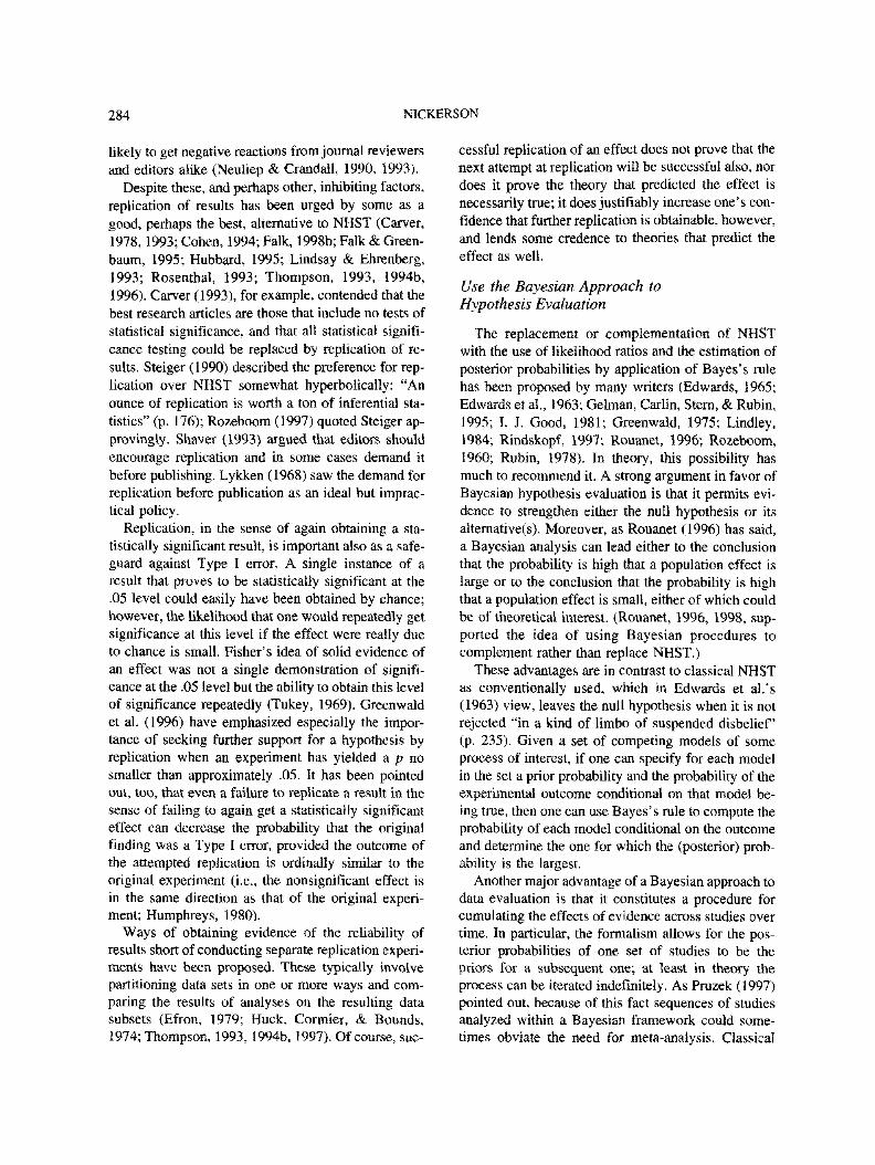
284 N1CKERSON
likely to get negative reactions from journal reviewers
and editors alike (Neuliep & Crandall, 1990, 1993).Despite these, and perhaps other, inhibiting factors,
replication of results has been urged by some as agood, perhaps the best, alternative to NHST (Carver,
1978,1993; Cohen, 1994; Falk, 1998b; Falk & Green-
baum, 1995; Hubbard, 1995; Lindsay & Ehrenberg,
1993; Rosenthal, 1993; Thompson, 1993, 1994b,1996). Carver (1993), for example, contended that the
best research articles are those that include no tests of
statistical significance, and that all statistical signifi-
cance testing could be replaced by replication of re-
sults. Steiger (1990) described the preference for rep-lication over NHST somewhat hyperbolically: "An
ounce of replication is worth a ton of inferential sta-
tistics" (p. 176); Rozeboom (1997) quoted Steiger ap-
provingly. Shaver (1993) argued that editors should
encourage replication and in some cases demand it
before publishing. Lykken (1968) saw the demand forreplication before publication as an ideal but imprac-tical policy.
Replication, in the sense of again obtaining a sta-tistically significant result, is important also as a safe-guard against Type I error. A single instance of aresult that proves to be statistically significant at the.05 level could easily have been obtained by chance;however, the likelihood that one would repeatedly getsignificance at this level if the effect were really dueto chance is small. Fisher's idea of solid evidence of
an effect was not a single demonstration of signifi-cance at the .05 level but the ability to obtain this levelof significance repeatedly (Tukey, 1969). Greenwaldet al. (1996) have emphasized especially the impor-tance of seeking further support for a hypothesis byreplication when an experiment has yielded a p no
smaller than approximately .05. It has been pointedout, too, that even a failure to replicate a result in thesense of failing to again get a statistically significanteffect can decrease the probability that the originalfinding was a Type I error, provided the outcome ofthe attempted replication is ordinally similar to theoriginal experiment (i.e., the nonsignificant effect isin the same direction as that of the original experi-ment; Humphreys, 1980).
Ways of obtaining evidence of the reliability ofresults short of conducting separate replication experi-ments have been proposed. These typically involvepartitioning data sets in one or more ways and com-paring the results of analyses on the resulting datasubsets (Efron, 1979; Huck, Cormier, & Bounds,1974; Thompson, 1993, 1994b, 1997). Of course, suc-
cessful replication of an effect does not prove that thenext attempt at replication will be successful also, nordoes it prove the theory that predicted the effect isnecessarily true; it does justifiably increase one's con-fidence that further replication is obtainable, however,
and lends some credence to theories that predict the
effect as well.
Use the Bayesian Approach to
Hypothesis Evaluation
The replacement or complementation of NHST
with the use of likelihood ratios and the estimation ofposterior probabilities by application of Bayes's rule
has been proposed by many writers (Edwards, 1965;Edwards et al., 1963; Gelman, Carlin, Stern, & Rubin,
1995; I. J. Good, 1981; Greenwald, 1975; Lindley,1984; Rindskopf, 1997; Rouanet, 1996; Rozeboom,
1960; Rubin, 1978). In theory, this possibility hasmuch to recommend it. A strong argument in favor ofBayesian hypothesis evaluation is that it permits evi-
dence to strengthen either the null hypothesis or itsalternative(s). Moreover, as Rouanet (1996) has said,a Bayesian analysis can lead either to the conclusionthat the probability is high that a population effect islarge or to the conclusion that the probability is highthat a population effect is small, either of which couldbe of theoretical interest. (Rouanet, 1996, 1998, sup-
ported the idea of using Bayesian procedures tocomplement rather than replace NHST.)
These advantages are in contrast to classical NHSTas conventionally used, which in Edwards et al.'s(1963) view, leaves the null hypothesis when it is notrejected "in a kind of limbo of suspended disbelief(p. 235). Given a set of competing models of someprocess of interest, if one can specify for each modelin the set a prior probability and the probability of theexperimental outcome conditional on that model be-ing true, then one can use Bayes's rule to compute theprobability of each model conditional on the outcomeand determine the one for which the (posterior) prob-ability is the largest.
Another major advantage of a Bayesian approach todata evaluation is that it constitutes a procedure forcumulating the effects of evidence across studies overtime. In particular, the formalism allows for the pos-terior probabilities of one set of studies to be thepriors for a subsequent one; at least in theory theprocess can be iterated indefinitely. As Pruzek (1997)pointed out, because of this fact sequences of studiesanalyzed within a Bayesian framework could some-times obviate the need for meta-analysis. Classical
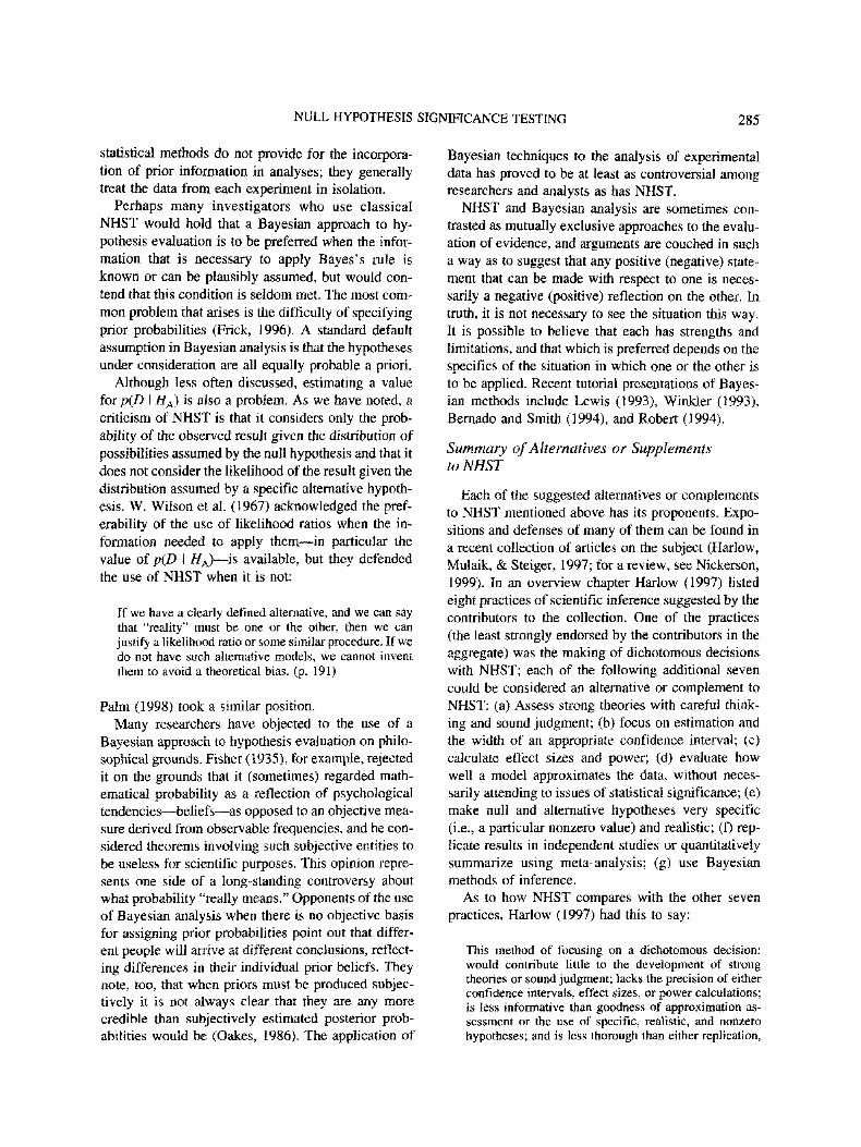
NULL HYPOTHESIS SIGNIFICANCE TESTING 285
statistical methods do not provide for the incorpora-
tion of prior information in analyses; they generally
treat the data from each experiment in isolation.
Perhaps many investigators who use classical
NHST would hold that a Bayesian approach to hy-
pothesis evaluation is to be preferred when the infor-
mation that is necessary to apply Bayes's rule is
known or can be plausibly assumed, but would con-
tend that this condition is seldom met. The most com-
mon problem that arises is the difficulty of specifying
prior probabilities (Frick, 1996). A standard default
assumption in Bayesian analysis is that the hypotheses
under consideration are all equally probable a priori.
Although less often discussed, estimating a value
for p(D \ HA) is also a problem. As we have noted, a
criticism of NHST is that it considers only the prob-
ability of the observed result given the distribution of
possibilities assumed by the null hypothesis and that it
does not consider the likelihood of the result given the
distribution assumed by a specific alternative hypoth-
esis. W. Wilson et al. (1967) acknowledged the pref-
erability of the use of likelihood ratios when the in-
formation needed to apply them—in particular the
value of p(D I #A)—is available, but they defended
the use of NHST when it is not:
If we have a clearly defined alternative, and we can say
that "reality" must be one or the other, then we can
justify a likelihood ratio or some similar procedure. If we
do not have such alternative models, we cannot invent
them to avoid a theoretical bias. (p. 191)
Palm (1998) took a similar position.
Many researchers have objected to the use of a
Bayesian approach to hypothesis evaluation on philo-
sophical grounds. Fisher (1935), for example, rejected
it on the grounds that it (sometimes) regarded math-
ematical probability as a reflection of psychological
tendencies—beliefs—as opposed to an objective mea-
sure derived from observable frequencies, and he con-
sidered theorems involving such subjective entities to
be useless for scientific purposes. This opinion repre-
sents one side of a long-standing controversy about
what probability "really means." Opponents of the use
of Bayesian analysis when there is no objective basis
for assigning prior probabilities point out that differ-
ent people will arrive at different conclusions, reflect-
ing differences in their individual prior beliefs. They
note, too, that when priors must be produced subjec-
tively it is not always clear that they are any more
credible than subjectively estimated posterior prob-
abilities would be (Oakes, 1986). The application of
Bayesian techniques to the analysis of experimental
data has proved to be at least as controversial among
researchers and analysts as has NHST.
NHST and Bayesian analysis are sometimes con-
trasted as mutually exclusive approaches to the evalu-
ation of evidence, and arguments are couched in such
a way as to suggest that any positive (negative) state-
ment that can be made with respect to one is neces-
sarily a negative (positive) reflection on the other. In
truth, it is not necessary to see the situation this way.
It is possible to believe that each has strengths and
limitations, and that which is preferred depends on the
specifics of the situation in which one or the other is
to be applied. Recent tutorial presentations of Bayes-
ian methods include Lewis (1993), Winkler (1993),
Bernado and Smith (1994), and Robert (1994).
Summary of Alternatives or Supplementsto NHST
Each of the suggested alternatives or complements
to NHST mentioned above has its proponents. Expo-
sitions and defenses of many of them can be found in
a recent collection of articles on the subject (Harlow,
Mulaik, £ Steiger, 1997; for a review, see Nickerson,
1999). In an overview chapter Harlow (1997) listed
eight practices of scientific inference suggested by the
contributors to the collection. One of the practices
(the least strongly endorsed by the contributors in the
aggregate) was the making of dichotomous decisions
with NHST; each of the following additional seven
could be considered an alternative or complement to
NHST: (a) Assess strong theories with careful think-
ing and sound judgment; (b) focus on estimation and
the width of an appropriate confidence interval; (c)
calculate effect sizes and power; (d) evaluate how
well a model approximates the data, without neces-
sarily attending to issues of statistical significance; (e)
make null and alternative hypotheses very specific
(i.e., a particular nonzero value) and realistic; (f) rep-
licate results in independent studies or quantitatively
summarize using meta-analysis; (g) use Bayesian
methods of inference.
As to how NHST compares with the other seven
practices, Harlow (1997) had this to say:
This method of focusing on a dichotomous decision:
would contribute little to the development of strongtheories or sound judgment; lacks the precision of either
confidence intervals, effect sizes, or power calculations;
is less informative than goodness of approximation as-sessment or the use of specific, realistic, and nonzero
hypotheses; and is less thorough than either replication,
286 NICKERSON
meta-analysis, or Bayesian inference... In sum, theoverriding view on this issue is that NHST may be over-used and unproductive, particularly when used as simplya dichotomous decision rule. (p. 12)
There can be little doubt that NHST has many crit-
ics and that there is general agreement among them
that the method, especially when used as the only
indicant of scientific credibility, is seriously flawed.
Harlow's (1997) negative summary of its weaknesses
was intended, I assume, to represent the overriding,
though not unanimous, view among the contributors
to Harlow et al.'s (1997) volume. The extent to which
that view prevails among the research community
more generally is not so clear.
Other Recommendations
In addition to recommendations pertaining directly
to the use of NHST or regarding specific alternative or
complementary approaches to data analysis, a number
of more general recommendations have been made or
could be made. I mention a few here that I think are
especially noteworthy.
Make a Clear Distinction Between theSubstantive Questions) of Interest and theStatistical Hypothesis(es) to Be Tested
Researchers should distinguish statistical from epistemicquestions, that is, when they are making an inferenceconcerning a parameter (point value, range, slope, sign)from a statistic versus when they are appraising the veri-similitude of a substantive theory (causal, compositional,or historical) on the basis of the inferred parameters.(Meehl, 1997, p. 422)
It seems to me that this recommendation by Meehl, if
followed carefully, would go a long way toward solv-
ing many of the problems associated with NHST. This
surmise is based on the assumption that at the root of
many of these problems is either a confusion between
epistemic and statistical hypotheses or a focus on the
latter type to the neglect of the former.
Make NHST Subsidiary to OtherConsiderations in Evaluating Data
Carver (1978, 1993) argued that testing for statis-
tical significance before considering whether the data
are generally supportive of the experimental hypoth-
esis of interest is a corruption of the scientific method
and that the rule should be to always interpret the
results with respect to the data first and do statistical
significance testing only secondarily. As to the argu-
ment that one may have to test for statistical signifi-
cance in order to see whether there is any effect worth
further consideration, Carver had little patience with
it: "A study with results that cannot be meaningfully
interpreted without looking at the p values is a poorly
designed study" (1978, p. 394).
A not dissimilar sentiment has been expressed by I.
J. Good (1981/1983b): "Personally I think that Rule 1
in the analysis of data is 'look at the data' " (p. 138).
Rozeboom (1997) encapsulated a closely related idea
in what he called "the statistical relevance precept,"
according to which one should think through what one
would want to make of a finding if one could obtain
data with no sampling error. "You have nothing to
gain from concern for a statistics sampling uncer-
tainty (save to oblique colleagues who want it) if you
have little idea of what to do with its population value
were you to know that" (p. 385). Rouanet (1996), who
argued strongly for the use of a Bayesian approach to
data analysis, also contended that one should consider
first whether an effect is sufficiently large (or suffi-
ciently small) to be of interest if it held for the rel-
evant population as well as for the sample before
doing any statistical analyses. "If this is not the case,
no corresponding inferential conclusion is reachable.
If this is the case, the aim ascribed to inferential pro-
cedures should be to extend descriptive conclusions to
the population, allowing for sampling fluctuations"
(p. 150).
Sohn (1998b) recommended that, at least in the
case of atheoretical research, findings should be taken
seriously only when they can be obtained consistently
with individuals. In effect this means they should be
discernible without the help of inferential statistics:
In the context of atheoretical research... effects need tobe so robust that they are discernible in the individualorganism so consistently that there is general agreementthat the treatment is producing an effect. In such a case,significance tests are supererogatory. (Sohn, 1998b, p.307)
Sohn (1998a) expressed the opinion that in psychol-
ogy "findings that are not obviously discernible in
nearly every instance are likely to be ignored. And if
they are not ignored, they typically become a source
of controversy" (p. 334).
What makes an experimental result worth publish-
ing is a matter of opinion. I suspect there are few
researchers who would argue that statistical signifi-
cance alone suffices, but one must wonder about the
extent to which fixation on NHST to the exclusion of
NULL HYPOTHESIS SIGNIFICANCE TESTING 287
other considerations has contributed to the "indis-
criminate cataloguing of trivial effects," which W.
Wilson et al. (1967) referred to 30 years ago as "a
major problem in psychology today" (p. 195). More
recently, Abelson (1997a, 1997b) has noted that sig-
nificance tests are sometimes applied in unthinking
ways to test differences that have little or no relevance
to the question of interest or that are apparent without
the benefit of the test.
The indiscriminate use of NHST has been criticized
in even stronger terms by Edwards (1965), who has
commented on what he considers to be the violent
bias of classical hypothesis testing against the null
hypothesis:
This violent bias of classical procedures is not an un-
mitigated disaster. Many null hypotheses tested by clas-
sical procedures are scientifically preposterous, not wor-thy of a moment's credence even as approximations. If a
hypothesis is preposterous to start with, no amount of
bias against it can be too great. On the other hand, if it
is preposterous to start with, why test it? (p. 402)
Sometimes statistics are used to compensate for
poorly controlled experimentation. Variables are var-
ied unsystematically, and little attention is given to
the possibility of artifactual effects, the assumption
being that statistical analyses will sort everything out.
However, it is precisely where statistics are most
needed to make sense of noisy data that significance
tests lend themselves most readily to misinterpretation
and misuse. As W. Wilson et al. (1967) said: "It
makes relatively little difference which approach you
use in precise experimentation. With great precision,
you cannot go too far wrong" (p. 194). Conversely,
given sloppy experimentation statistics are at least as
likely to obfuscate as to clarify.
To keep NHST and other statistical procedures in
perspective, it is well to also bear in mind that much
scientifically solid and exceptionally influential psy-
chological research has been done with relatively
little, if any, use of statistics. The names of James,
Bartlett, Piaget, Skinner, and Wertheimer come im-
mediately to mind. Moreover, even effects that are
statistically significant at a small value of p—and are
large—are not guaranteed to be interesting and im-
portant; these aspects can be determined only relative
to some value system that is beyond the province of
statistics. A single-minded concern for statistical sig-
nificance untempered by other considerations does
not serve the best interests of any scientific field.
Consider the Intended User of theResearch Findings
I have appropriated this recommendation from C.
D. Wickens (1998) because it seems to me an obvi-
ously correct and important but neglected point. I sus-
pect that most participants in the debate about NHST
assume that the primary audience for research reports
is other researchers, but potential users of the results
of applied research include people other than re-
searchers. What is most helpful by way of statistical
analyses and statistical reporting for researchers may
not necessarily be what is most helpful for practitio-
ners. For example, while the conservative policy of
guarding against Type I error at the expense of allow-
ing a high incidence of Type II error may be in keep-
ing with the idea that novel hypotheses should not be
accepted or old ones discarded except on "beyond-a-
reasonable-doubt" evidence, when a decision must be
made between two possible approaches to a practical
problem and the costs of both possible errors are com-
parable, a "preponderance-of-evidence" criterion may
be more appropriate.
Understand (Perhaps Even Explain) StatisticalApproach and Rationale for It
Whatever approach one takes to hypothesis evalu-
ation, it seems a good idea to understand why one is
taking that approach. It is at least a plausible conjec-
ture that many users of statistical tests lack a deep
conceptual grasp of the logic of those tests, the con-
ditions that legitimize their use, and the conclusions
they justify. The main effects of such lack of under-
standing are likely to be misapplication of tests and
the drawing of unsubstantiated conclusions from their
outcomes; and they can only be magnified by the
ready availability of software that makes statistical
tests—whether appropriate or not—trivially easy to
perform.
Not only is understanding of the statistical tests one
uses important, sometimes it may be desirable to ex-
plain the rationale for one's statistical approach. This
may mean stating any important assumptions that will
not be obvious to the reader. If, for example, one is
using a point null hypothesis as a convenient proxy
for a range null, it would help to make this clear and
to specify the range. It also means being explicit about
how a statistic was computed when more than one
method is possible and the different methods yield
different results.
288 NICKERSON
Choose Language Carefully
Undoubtedly some of the misconceptions about
NHST are maintained and reinforced by the use of
less-than-precise language in discussions of NHST
and the results of such testing. The word significance
invites misconception in the statistical context be-
cause of its everyday connotation of importance.
Some writers have suggested discontinuing use of the
word to convey statistical meaning—Chow (1996),
for example, suggested replacing it with nonchance—
but it seems unlikely that the term will disappear from
psychologists' vocabularies anytime soon. Some writ-
ers use reliable in lieu of statistically significant, but
this could be interpreted as assuredly replicable.
Reporting statistical significance as simply "signifi-
cance" undoubtedly contributes to the confusion be-
tween statistical significance and importance from a
theoretical or practical point of view. This is not to
suggest that one needs slavishly to qualify every in-
stance of reporting the results of a statistical signifi-
cance test with the word statistical, which can become
tediously repetitive in some cases, but it is to suggest
that one should be careful to make it clear that statis-
tical significance—as opposed to theoretical or prac-
tical significance—is intended whenever there is a
good chance of misinterpretation.
Careful use of language is especially important
when speaking of conditional probabilities having to
do with NHST. Reference to the a level as "the prob-
ability of Type I error" without making clear that it is
the probability of rejecting H0 conditional on H0 be-
ing true illustrates the point, as does reference to |J as
"the probability of Type II error" without explicitly
noting that |3 is the probability of failing to reject HQ
conditional on H0 being false. There are many other
possibilities for confusion arising from failure to note
the conditional status of probabilities, some of which
have been mentioned in preceding sections of this
article.
After writing the preceding paragraph, I checked
some definitions in the fifth edition of a statistics text
of some longevity (Witte & Witte, 1997) that hap-
pened to be within reach. I found the following state-
ments: "Alpha (a): The probability of a type I error,
that is, the probability of rejecting a true null hypoth-
esis" (p. 251). "Beta ((B): The probability of a type II
error, that is, the probability of retaining a false null
hypothesis" (p. 253). "Power (l-p5): The probability
of detecting a particular effect" (p. 258). Each of the
probabilities mentioned is a conditional probability. 1
am sure that Witte and Witte understand this and per-
haps a careful reading of the entire presentation in the
text would make the conditionality clear, but the defi-
nitions lend themselves to misinterpretation.
Consider Aggregate Evidence
NHST is usually done with respect to the outcome
of a single experiment or the manipulation of a single
experimental variable. As has been pointed out many
times, few psychologists would be willing to decide
on the truth or falsity or general tenability of a hy-
pothesis of nontrivial interest on the basis of the out-
come of a single experiment. What seems to happen is
that researchers are persuaded of the tenability or un-
tenability of a hypothesis by the accumulation of evi-
dence for or against it over many different experi-
ments. The impact of the outcome of a single
experiment depends in part on the prior tenability of
the hypothesis because of evidence in hand before the
experiment was done. According to a Bayesian view,
this is as it should be.
The use of meta-analytic techniques has been urged
by many as a structured method for considering the
implications of the results of sets of experiments in
the aggregate (Cooper, 1979; Cooper & Rosenthal,
1980; Eddy, Hasselblad, & Shachter, 1992; Glass,
1976; Glass & Kliegl, 1983; Hunter & Schmidt, 1990;
Hunter, Schmidt, & Jackson, 1982; Schmidt, 1992,
1996). Meta-analysis has the advantage, its propo-
nents argue, that it provides a means of extracting
useful information even from the results of experi-
ments that have not been statistically significant on
their own. Even Mulaik et al. (1997), who strongly
defended the use of NHST, recommend that in evalu-
ating studies journal editors consider the potential of
their data being useful in combination with those of
other studies in meta-analyses. Schmidt and Hunter
(1997) argued that single studies do not contain
enough information to be decisive with respect to hy-
potheses and that it is only by combining the findings
of individual studies through the use of meta-analysis
that dependable scientific conclusions can be reached.
They went so far as to suggest that
from the point of view of the goal of optimally advanc-
ing the cumulation of scientific knowledge, it is best for
individual researchers to present point estimates and
confidence intervals and refrain from attempting to drawfinal conclusions about research hypotheses. These will
emerge from later meta-analyses. (p. 52)
Without denying the importance of analytic tech-
niques for aggregating the results of a large number of
NULL HYPOTHESIS SIGNIFICANCE TESTING 289
experiments, I believe that individual experiments and
their stand-alone results will continue to play a critical
role in the advance of psychological knowledge. I can
do no better than quote Abelson (1997b) on this point:
"Even though a single study cannot strictly prove any-
thing, it can challenge, provoke, irritate, or inspire
further research to generalize, elaborate, clarify, or to
debunk the claims of the single study" (p. 124). We
need to also bear in mind that it is possible for knowl-
edge to cumulate without the aid of specific meta-
analytic techniques; it has done so in the physical
sciences quite effectively for a long time. Moreover,
meta-analysis is not entirely free of problems and of-
fers its own set of possibilities for misuse (Chow,
1996; Erwin, 1997; Gallo, 1978; Knight, Fabes, &
Higgins, 1996; Lepper, 1995; Leviton & Cook, 1981;
Shapiro, 1997; Sohn, 1996: G. T. Wilson & Rachman,
1983).
Recognize the Provisional Natureof Hypotheses
In their defense of NHST, Mulaik et al. (1997)
emphasized—following Fisher (1935)—the impor-
tance of recognizing the tenability or defeasibility of
scientific hypotheses or generalizations. All hypoth-
eses, no matter what the evidence respecting them at
any given time, are subject to modification as a con-
sequence of further information that is relevant to
them.
Conclusion
NHST has been and is a controversial method of
extracting information from experimental data and of
guiding the formation of scientific conclusions. As
Meehl (1997) said:
Competent scholars persist in strong disagreement, rang-ing from some who think W0-testing is pretty much allright as practiced, to others who think it is never appro-priate. Most critics fall somewhere between these ex-tremes, and they differ among themselves as to theirmain reasons for complaint, (p. 421)
"Strong disagreement" does not quite capture the
intensity of some of the contributions to the debate.
Although many of the participants have stated their
positions objectively and gracefully, I have been
struck with the stridency of the attacks by some on
views that oppose their own. NHST has been de-
scribed as "thoroughly discredited," a "perversion of
the scientific method," a "bone-headedly misguided
procedure," "grotesquely fallacious," a "disaster," and
"mindless," among other things. Positions, pro or con,
have been labeled "absurd," "senseless," "nonsensi-
cal," "ridiculous," and "silly." The surety of the pro-
nouncements of some participants on both sides of the
debate is remarkable.
One hypothesis worth entertaining about the con-
troversy is that it is a tempest in a teapot. (I am re-
minded of a comment by Kac, 1964: "Whatever your
views and beliefs on randomness—and they are more
likely than not untenable—no great harm will come to
you.") Perhaps a case could be made for this possi-
bility. What is the great harm if many people who use
NHST believe that p is the probability that the null
hypothesis is true, or that a small p is evidence of
replicability, or that a is the probability that if one has
rejected the null hypothesis one has made a Type I
error? Claims to the contrary notwithstanding, there is
room for doubt as to whether acquisition of psycho-
logical knowledge through experimentation has been
greatly impeded by the prevalence of such beliefs or
by any of the many other shortcomings of NHST that
have been ably identified by its critics.
Moreover, evidence suggests that the confidence
psychologists place in experimental findings tends to
vary with statistical test outcomes in intuitively rea-
sonable ways. Confidence generally varies inversely
with p value and directly with effect size and sample
size (Beauchamp & May, 1964; Nelson et al., 1986;
Rosenthal & Gaito, 1963, 1964). Confidence in a
finding is also increased as a consequence of success-
ful replication (Nelson et al., 1986). Despite the many
problems associated with NHST, these predilections
should facilitate orderly application of research results
to the advance of psychological theory. Most impor-
tantly, under assumptions that may be valid for most
experiments, a small value of p is indeed indicative of
a not-quite-so-small value of p(H0 I D). Perhaps it is
the case, as Rindskopf (1997) has argued, that null
hypothesis tests are still used because "they are testing
approximately the right thing under many real circum-
stances, even though most researchers do not know
the rationale" (p. 321).
On the other hand, as noted at the outset, NHST is
arguably the most widely used method of analysis of
data collected in psychological experiments and has
been so for a long time. If it is misunderstood by
many of its users in as many ways as its critics claim,
this is an embarrassment for the field. A minimal goal
for experimental psychology should be to attempt to
achieve a better understanding among researchers of
the approach, of its strengths and limitations, of the
290 NICKERSON
various objections that have been raised against it, and
of the assumptions that are necessary to justify spe-
cific conclusions that can be drawn from its results.
The situation is not simple—it is confused and con-
fusing—and a nonsuperficial understanding of the is-
sues requires a considerable investment of time and
effort. Having made a bit of an effort in this direction
myself, one conclusion that I have come to is that it is
not necessarily the case that the more one learns about
NHST, the clearer its proper role in psychological
research becomes; a more likely consequence of
learning, in my view, is the discovery that some of the
principles and relationships one had considered well-
established or that one had taken for granted are not
beyond dispute. One finds conflicting opinions
strongly held by knowledgeable people on various
aspects of the topic, and it is not always easy to be
sure of what one's own should be. However, there is
little virtue in being confident of one's opinions when
the confidence depends on not being aware of rea-
soned alternatives that exist.
The debate about NHST has its roots in unresolved
disagreements among major contributors to the devel-
opment of theories of inferential statistics on which
modern approaches are based. Gigerenzer et al.
(1989) have reviewed in considerable detail the con-
troversy between R. A. Fisher on the one hand and
Jerzy Neyman and Egon Pearson on the other as well
as the disagreements between both of these views and
those of the followers of Thomas Bayes. They noted
the remarkable fact that little hint of the historical and
ongoing controversy is to be found in most textbooks
that are used to teach NHST to its potential users. The
resulting lack of an accurate historical perspective and
understanding of the complexity and sometimes con-
troversial philosophical foundations of various ap-
proaches to statistical inference may go a long way
toward explaining the apparent ease with which sta-
tistical tests are misused and misinterpreted.
On one point most writers agree: NHST cannot be
done mechanically without running the risk of obtain-
ing nonsensical results; human judgment must be an
integral, and controlling, aspect of the process. Abel-
son (1997a) made this point forcefully:
Whatever else is done about null-hypothesis tests, let usstop viewing statistical analysis as a sanctification pro-cess. We are awash in a sea of uncertainty, caused by aflood tide of sampling and measurement errors, and thereare no objective procedures that avoid human judgmentand guarantee correct interpretations of results, (p. 13)
To the extent that the motivation to ban NHST stems
from a desire to rid psychology or psychologists of
misconceptions of the sort reviewed in the first part of
this article, there is little reason to believe that such a
ban would have the desired effect because the pro-
posed alternatives to NHST lend themselves to mis-
interpretations and misuses as well. As R. J. Harris
(1997a) said: "Banning significance tests is clearly
not going to guarantee that misunderstandings of the
role of sampling error and the strength of evidence
required to establish the validity of a null hypothesis
won't continue to bedevil us" (p. 160). NHST surely
has warts, but so do all the alternatives.
The indispensability of human judgment in the in-
terpretation of the results of research, including the
results of statistical tests, has been stressed by many
(Berger & Berry, 1988; Browne & Cudek, 1992; Co-
hen, 1994; Cortina & Dunlap, 1997; Falk & Green-
baum, 1995; Gigerenzer, 1993; Huberty & Morris,
1988; Malgady, 1998). However, judicious use of sta-
tistical tests presupposes a level of mathematical so-
phistication that the training of social scientists often
fails to achieve, and lack of this sophistication
coupled with the ready availability of statistical soft-
ware more or less ensures some inappropriate appli-
cations of statistical tests and unreasoned uses of their
results (Estes, 1997b).
Arguments regarding the appropriateness of NHST
will surely continue. Most Bayesians will undoubt-
edly argue against it, and many non-Bayesians will
continue to use it; but this split is too simple. There
are people who see the advantages of Bayesian analy-
sis when the information that it requires is readily at
hand who are not ready to declare NHST defunct. I. J.
Good (1981/1983b) has put himself in this camp:
I personally am in favor of a Bayes/non-Bayes compro-mise or synthesis. Partly for the sake of communicationwith other statisticians who are in the habit of usingtail-area probabilities, 1 believe it is often convenient touse them especially when it is difficult to estimate aBayes factor. But caution should be expressed when thesamples are very large if the tail-area probability is notextremely small, (p. 143)
McGrath (1998) has argued that it is not a question
of whether NHST is useless but rather whether there
is something better. This is a question that should be
asked, in my view, whenever one is attempting to
decide how to extract information from data, and it
applies not only to NHST but to any other approach
one might consider using. There are no statistical pro-
NULL HYPOTHESIS SIGNIFICANCE TESTING 291
cedures that can safely be used without thought as to
their appropriateness to the situation or the question of
whether there are more effective approaches avail-
able. Statistical methods should facilitate good think-
ing, and only to the degree that they do so are they
being used well. When applied unthinkingly in cook-
book fashion and without awareness of their limita-
tions and of the assumptions that are needed to justify
conclusions drawn from them, they can get in the way
of productive reasoning; when used judiciously, with
cognizance of their limitations, they can be very help-
ful in making sense of data and determining what
conclusions are justified. NHST, like other statistical
tools, can be applied in inappropriate and counterpro-
ductive ways—easily when its rules of application or
its products are not well understood—but it can also
be an effective aid to data interpretation when used
appropriately as an adjunct to good experimental de-
sign and in conjunction with other methods of extract-
ing information from noisy data.
Finally, in trying to assess the merits of NHST and
other approaches to the evaluation of hypotheses, it is
well to bear in mind that nothing of importance in
psychology has ever been decided on the basis of the
outcome of a single statistical significance test. Psy-
chological knowledge is acquired, as is knowledge in
other fields, as a consequence of the cumulative effect
of many experiments and nonexperimental observa-
tions as well. It is the preponderance of evidence gath-
ered from many sources and over an extended period
of time that determines the degree of credibility that is
given to hypotheses, models, and theories.
References
Abelson, R. P. (1995). Statistics as principled argument.
Hillsdale, NJ: Erlbaum.
Abelson, R. P. (1997a). On the surprising longevity of
flogged horses: Why there is a case for the significance
test. Psychological Science, 8, 12-15.
Abelson, R. P. (1997b). A retrospective on the significance
test ban of 1999 (if there were no significance tests, they
would be invented). In L. L. Harlow, S. A. Mulaik, &
J. H. Steiger (Eds.), What if there were no significance
tests? (pp. 117-141). Hillsdale, NJ: Erlbaum.
American Psychological Association. (1994). Publication
manual of the American Psychological Association (4th
ed.). Washington, DC: Author.
Anastasi, A. (1988). Psychological testing (6th ed.). New
York: Macmillan.
Asher, W. (1993). The role of statistics in research. Journal
of Experimental Education, 61, 388-393.
Atkinson, D. R., Furlong, M. J., & Wampold, B. E. (1982).
Statistical significance, reviewer evaluations, and scien-
tific process: Is there a (statistically) significant relation-
ship? Journal of Counseling Psychology, 29, 189-194.
Bailer, J. C., & Mosteller, F. (1988). Guidelines for statis-
tical reporting in articles for medical journals: Amplifi-
cations and explanations. Annals of Internal Medicine,
108, 266-273.
Bakan, D. (1966). The test of significance in psychological
research. Psychological Bulletin, 66, 423^37.
Bar-Hillel, M. A. (1974). Similarity and probability. Orga-
nizational Behavior and Human Performance, 11, 277-
282.
Bar-Hillel, M. A., & Falk, R. (1982). Some teasers concern-
ing conditional probabilities. Cognition, II, 109-122.
Baril, G. L., & Cannon, J. T. (1995). What is the probability
that null hypothesis testing is meaningless? American
Psychologist, 50, 1098-1099.
Bartko, J. J. (1991). Proving the null hypothesis. American
Psychologist, 46, 1089.
Beauchamp, K. L., & May, R. B. (1964). Replication report:
Interpretation of levels of significance by psychological
researchers. Psychological Reports, 14, 272.
Berger, J. O., & Berry, D. A. (1988). Statistical analysis and
the illusion of objectivity. American Scientist, 76, 159-
165.
Berger, J. O., & Sellke, T. (1987). Testing a point null hy-
pothesis: The irreconcilability of P values and evidence.
Journal of the American Statistical Association, 82, 112-
122.
Berkson, J. (1938). Some difficulties of interpretation en-
countered in the application of the chi-square test. Jour-
nal of the American Statistical Association, 33, 526-542.
Berkson, J. (1942). Tests of significance considered as evi-
dence. Journal of the American Statistical Association,
37, 325-335.
Bernado, J. M., & Smith, A. F. M. (1994). Bayesian theory.
New York: Wiley.
Bhattacharyya, G. K., & Johnson, R. A. (1977). Statistical
concepts and methods. New York: Wiley.
Binder, A. (1963). Further considerations on testing the null
hypothesis and the strategy and tactics of investigating
theoretical models. Psychological Review, 70, 107-115.
Birnbaum, I. (1982). Interpreting statistical significance.
Teaching Statistics, 4, 24-26.
Blaich, C. F. (1998). The null-hypothesis significance test
procedure: Can't live with it, can't live without it. Be-
havioral and Brain Sciences, 21, 194-195.
Bohrer, R. (1979). Multiple three-decision rules for para-
292 NICKERSON
metric signs. Journal of the American Statistical Asso-
ciation, 74, 432^37.
Bolles, R. C. (1962). The difference between statistical hy-
potheses and scientific hypotheses. Psychological Re-
parts, 11, 639-645.
Bolles, R. C., & Messick, S. (1958). Statistical utility in
experimental inference. Psychological Reports, 4, 223-
227.
Bookstein, F. L. (1998). Statistical significance testing was
not meant for weak corroboration of weaker theories.
Behavioral and Brain Sciences, 21, 195-196.
Borowski, E. J., & Borwein, I. M. (1991). The Harper Col-
lins dictionary of mathematics. New York: Harper Col-
lins.
Bracey, G. W. (1991). Sense, non-sense, and statistics. Phi
Delta Kappan, 73, 335.
Braver, S. L. (1975). On splitting the tails unequally: A new
perspective on one versus two-tailed tests. Educational
and Psychological Measurement, 35, 283-301.
Brewer, J. K. (1985). Behavioral statistics textbooks:
Source of myths and misconceptions? Journal of Educa-
tional Statistics, 10, 252-268.
Browne, M. W., & Cudek, R. C. (1992). Alternative ways
of assessing model fit. Sociological Methods and Re-
search, 21, 230-258.
Carver, R. P. (1978). The case against statistical signifi-
cance testing. Harvard Educational Review, 48, 378-399.
Carver, R. P. (1993). The case against statistical signifi-
cance testing, revisited. Journal of Experimental Educa-
tion, 61, 287-292.
Cassells, W., Schoenberger, A., & Graboys, T. B. (1978).
Interpretation by physicians of clinical laboratory results.
The New England Journal of Medicine, 299, 999-1001.
Chase, L. J., & Tucker, R. K. (1976). Statistical power:
Derivation, development, and data-analytic implications.
Psychological Record, 26, 473-486.
Chow, S. L. (1987). Experimental psychology: Rationale,
procedures and issues. Calgary, Alberta, Canada: Detse-
lig Enterprises.
Chow, S. L. (1988). Significance test or effect size? Psy-
chological Bulletin, 103, 105-110.
Chow, S. L. (1989). Significance tests and deduction: Reply
to Folger (1989). Psychological Bulletin, 106, 161-165.
Chow, S. L. (1991). Some reservations about power analy-
sis. American Psychologist, 46, 1088-1089.
Chow, S. L. (1996). Statistical significance: Rationale, va-
lidity, and utility. Beverly Hills, CA: Sage.
Chow, S. L. (1998a), Precis of statistical significance: Ra-
tionale, validity, and utility. Behavioral and Brain Sci-
ences, 21, 169-239.
Chow, S. L. (1998b). What statistical significance means.
Theory and Psychology, 8, 323-330.
Clark, C. A. (1963). Hypothesis testing in relation to statis-
tical methodology. Review of Educational Research, 33,
455^473.
Clark, H. H. (1976). Reply to Wike and Church. Journal of
Verbal Learning and Verbal Behavior, 15, 257-261.
Clark-Carter, D. (1997). The account taken of statistical
power in research published in the British Journal of
Psychology. British Journal of Psychology, 88, 71-83.
Cliff, N. (1993). Dominance statistics: Ordinal analyses to
answer ordinal questions. Psychological Bulletin. 114,
494-509.
Cohen, J. (1962). The statistical power of abnormal-social
psychological research: A review. Journal of Abnormal
and Social Psychology, 69, 145-153.
Cohen, J. (1965). Some statistical issues in psychological
research. In B. B. Wolman (Ed.), Handbook of clinical
psychology (pp. 95-121). New York: McGraw-Hill.
Cohen, J. (1977). Statistical power analysis for the behav-
ioral sciences (Rev. ed.). New York: Academic Press.
Cohen, J. (1988). Statistical power analysis for the behavior
sciences (2nd ed.). Hillsdale, NJ: Erlbaum.
Cohen, J. (1990). Things I have learned (so far). American
Psychologist, 45, 1304-1312.
Cohen, J. (1994). The earth is round (p < .05). American
Psychologist, 49, 997-1003.
Cohen, J. (1995). The earth is round (p < .05): Rejoinder.
American Psychologist, 50, 1103.
Cohen, J., & Cohen, P. (1983). Applied multiple regression/
correlation analysis for the behavioral sciences (2nd ed.).
Hillsdale, NJ: Erlbaum.
Coleman, E. B. (1964). Generalizing to a language popula-
tion. Psychological Reports, 14, 219-226.
Cook, T. D., & Campbell, D. T. (1979). Quasi-experimen-
tation: Design and analysis issues for field settings. Chi-
cago: Rand McNally.
Cooper, H. M. (1979). Statistically combining independent
studies: A meta-analysis of sex differences in conformity
research. Journal of Personality and Social Psychology,
37, 131-146.
Cooper, H. M., & Rosenthal, R. (1980). Statistical versus
traditional procedures for summarizing research findings.
Psychological Bulletin, 87, 442-449.
Cortina, J. M., & Dunlap, W. P. (1997). On the logic and
purpose of significance testing. Psychological Methods,
2, 161-172.
Cowles, M., & Davis, C. (1982). On the origins of the .05
level of statistical significance. American Psychologist,
37, 553-558.
Cox, D. R. (1958). Some problems connected with statisti-
NULL HYPOTHESIS SIGNIFICANCE TESTING 293
cal inference. Annals of Mathematical Statistics, 29, 357-
372.
Cox, D. R. (1977). The role of significance tests. Scandi-
navian Journal of Statistics, 4, 49-70.
Cronbach, L. J. (1975). Beyond the two disciplines of sci-
entific psychology. American Psychologist, 30, 116-127.
Cronbach, L. J., & Snow, R. E. (1977). Aptitudes and in-
structional methods: A handbook for research on inter-
actions. New York: Irvington.
Crow, E. L. (1991). Response to Rosenthal's comment
"How are we doing in soft psychology?" American Psy-
chologist, 46, 1083.
Dar, R. (1987). Another look at Meehl, Lakatos, and the
scientific practices of psychologists. American Psycholo-
gist, 42, 145-151.
Dar, R. (1998). Null hypothesis tests and theory corrobora-
tion: Defending NHTP out of context. Behavioral and
Brain Sciences, 21, 196-197.
Dar, R., Serlin, R. C., & Omer, H. (1994). Misuse of sta-
tistical tests in three decades of psychotherapy research.
Journal of Consulting and Clinical Psychology, 62, 75-
82.
Darlington, R. B., & Carlson, P. M. (1987). Behavioral sta-
tistics: Logic and methods. New York: Free Press.
Dawes, R. M. (1988). Rational choice in an uncertain
world. San Diego, CA: Harcourt Brace Jovanovich.
Dawes, R. M., Mirels, H. L., Gold, E., & Donahue, E.
(1993). Equating inverse probabilities in implicit person-
ality judgments. Psychological Science, 4, 396-400.
DeGroot, M. H. (1973). Doing what comes naturally: Inter-
preting a tail area as a posterior probability or as a like-
lihood ratio. Journal of the American Statistical Associa-
tion. 68, 966-969.
DeGroot, M. H. (1982). Comment [on Shafer, 1982]. Jour-
nal of the American Statistical Association, 77, 336-339.
Dickey, J. M. (1973). Scientific reporting and personal
probabilities: Student's hypothesis. Journal of the Royal
Statistical Society, Series B, 285-305.
Dickey, J. M. (1977). Is the tail area useful as an approxi-
mate Bayes factor? Journal of the American Statistical
Association, 72, 138-142.
Dixon, P. (1998). Why scientists value p values. Psycho-
nomic Bulletin and Review, 5, 390-396.
Dracup, C. (1995). Hypothesis testing—What it really is.
The Psychologist, 8, 359-362.
Dunn, O. J. (1961). Multiple comparisons among means.
Journal of the American Statistical Association, 56, 52—
64.
Eddy, D. M. (1982). Probabilistic reasoning in clinical
medicine: Problems and opportunities. In D. Kahneman,
P. Slovic, & A. Tversky (Eds.), Judgment under uncer-
tainty: Heuristics and biases (pp. 249-267). Cambridge,
UK: Cambridge University Press.
Eddy, D. M., Hasselblad, V., & Shachter, R. (1992). Meta-
analysis by the confidence profile method: The statistical
synthesis of evidence. San Diego, CA: Academic Press.
Edgington, E. S. (1966). Statistical inference and nonran-
dom samples. Psychological Bulletin, 66, 485-487.
Edgington, E. S. (1995). Randomization tests (3rd ed.). New
York: Marcel Dekker.
Edwards, W. (1965). Tactical note on the relation between
scientific and statistical hypotheses. Psychological Bulle-
tin, 63, 400-402.
Edwards, W., Lindman, H., & Savage, L. J. (1963). Bayes-
ian statistical inference for psychological research. Psy-
chological Review, 70, 193-242.
Efron, B. (1979). Bootstrap methods: Another look at the
jackknife. Annals of Statistics, 7, 1-26.
Elifson, K. W., Runyon, R. P., & Haber, A. (1990). Funda-
mentals of social statistics. New York: McGraw-Hill.
English, H. B., & English, A. C. (1958). A comprehensive
dictionary of psychological and psychoanalytic terms.
New York: David McKay.
Erwin, E. (1997). Philosophy and psychotherapy: Razing
the troubles of the brain. Thousand Oaks, CA: Sage.
Erwin, E. (1998). The logic of null hypothesis testing. Be-
havioral and Brain Sciences, 21, 197-198.
Estes, W. K. (1997a). On the communication of information
by displays of standard errors and confidence intervals.
Psychonomic Bulletin and Review, 4, 330-341.
Estes, W. K. (1997b). Significance testing in psychological
research: Some persisting issues. Psychological Science,
8, 18-19.
Evans, J. D. (1985). Invitation to psychological research.
New York: Holt, Rinehart & Winston.
Eysenck, H. J. (1960). The concept of statistical signifi-
cance and the controversy about one-tailed tests. Psycho-
logical Review, 67, 269-271.
Falk, R. (1986). Misconceptions of statistical significance.
Journal of Structural Learning, 9, 83—96.
Falk, R. (1992). A closer look at the probabilities of the
notorious three prisoners. Cognition, 43, 197-223.
Falk, R. (1998a). In criticism of the null hypothesis statis-
tical test. American Psychologist, 53, 798-799.
Falk, R. (1998b). Replication—A step in the right direction.
Theory and Psychology, 8, 313-321.
Falk, R., & Greenbaum, C. W. (1995). Significance tests die
hard: The amazing persistence of a probabilistic miscon-
ception. Theory and Psychology, 5, 75-98.
Feinberg, W. E. (1971). Teaching Type-I and Type-IT er-
rors: The judicial process. The American Statistician, 25,
30-32.
294 NICKERSON
Fisher, R. A. (1925). Statistical methods for research work-
ers. London: Oliver & Boyd.
Fisher, R. A. (1935). The design of experiments. New York:
Hafner.
Fisher, R. A. (1956). Mathematics of a lady tasting tea. In
J. R. Newman (Ed.), The world of mathematics (pp.
1512-1521). New York: Simon & Schuster. (Original
work published 1935)
Fisher, R. A. (1990). Statistical methods and scientific in-
ference. New York: Oxford University Press. (Original
work published 1956)
Fleiss, J. L. (1969). Estimating the magnitude of experimen-
tal effects. Psychological Bulletin, 72, 273-276.
Folger, R. (1989). Significance tests and the duplicity of
binary decisions. Psychological Bulletin, 106, 155-160.
Fowler, R. L. (1985). Testing for substantive significance in
applied research by specifying nonzero effect null hy-
potheses. Journal of Applied Psychology, 70, 215-218.
Freiman, J. A., Chalmers, T. C., Smith, H., Jr., & Kuebler,
R. R. (1978). The importance of beta, the Type II error
and sample size in the design and interpretation of the
randomized control trial. New England Journal of Medi-
cine, 299, 690-694.
Freund, J. E. (1962). Mathematical statistics. Englewood
Cliffs, NJ: Prentice Hall.
Frick, R. W. (1995a). Accepting the null hypothesis.
Memory & Cognition, 23, 132-138.
Frick, R. W. (1995b). A problem with confidence intervals.
American Psychologist, 50, 1102-1103.
Frick, R. W. (1996). The appropriate use of null hypothesis
testing. Psychological Methods, 1, 379-390.
Frick, R. W. (1998). A better stopping rule of conventional
statistical tests. Behavior Research Methods, Instruments,
and Computers, 30, 690-697.
Friedman, H. (1968). Magnitude of experimental effect and
a table for its rapid estimation. Psychological Bulletin,
70, 245-251.
Gallo, P. S., Jr. (1978). Meta-analysis: A mixed meta-phor?
American Psychologist, 33, 515-517.
Gardner, M. J., & Airman, D. 0. (1986). Confidence inter-
vals rather than p values: Estimation rather than hypoth-
esis testing. British Medical Journal. 292, 746-750.
Garner, W. R., Hake, H. W., & Eriksen, C. W. (1956). Op-
erationalism and the concept of perception. Psychological
Review, 63, 149-159.
Gelman, A., Carlin, J., Stern, H., & Rubin, D. B. (1995).
Bayesian data analysis. London: Chapman & Hall.
Gibbons, J. D., & Pratt, J. W. (1975). P-values: Interpreta-
tion and methodology. American Statistician, 29, 20-25.
Giere, R. N. (1972). The significance test controversy. Brit-
ish Journal for the Philosophy of Science, 23, 170-181.
Gigerenzer, G. (1993). The Superego, the Ego, and the Id in
statistical reasoning. In G. Keren & C. Lewis (Eds.), A
handbook for data analysis in the behavioral sciences:
Methodological issues (pp. 311-339). Hillsdale, NJ:
Erlbaum.
Gigerenzer, G. (1998a). Surrogates for theories. Theory and
Psychology, 8, 195-204.
Gigerenzer, G. (1998b). We need statistical thinking, not
statistical rituals. Behavioral and Brain Sciences, 21,
199-200.
Gigerenzer, G., Hoffrage, U., & Ebert, A. (1998). AIDS
counseling for low-risk clients. AIDS Care, 10, 197-211.
Gigerenzer, G., & Murray, D. J. (1987). Cognition as intu-
itive statistics. Hillsdale, NJ: Erlbaum.
Gigerenzer, G., Swijtink, Z., Porter, T., Daston, L., Beatty,
J., & Kriiger, L. (1989). The empire of chance: How
probability changed science and everyday life. New
York: Cambridge University Press.
Gillman, L. (1992). The car and the goats. American Math-
ematical Monthly, 99, 3-7.
Glass, G. V. (1976). Primary, secondary, and meta-analysis
of research. Educational Researcher, 5(10), 3-8.
Glass, G. V., & Kliegl, R. M. (1983). An apology for re-
search integration in the study of psychotherapy. Journal
of Consulting and Clinical Psychology, 51, 28—41.
Glass, G. V., McGaw, B., & Smith, M. L. (1981). Meta-
analysis in social research. Beverly Hills, CA: Sage.
Gold, D. (1969). Statistical tests and substantive signifi-
cance. The American Sociologist, 4, 42-46.
Gonzalez, R. (1994). The statistics ritual in psychological
research. Psychological Science, 5, 321, 325-328.
Good, I. J. (1950). Probability and the weighing of evi-
dence. New York: Hafner.
Good, 1. J. (1956). Discussion of paper by G. Spencer
Brown. In Colin Cherry (Ed.), Information theory: Third
London Symposium (pp. 13—14). London: Butterworth.
Good, I. J. (1981). Some logic and history of hypothesis
testing. In J. Pitt (Ed.), Philosophy in economics (pp.
149-174). Dordrecht, The Netherlands: Reidel.
Good, I. J. (1982). Comment [on Shafer, 1982]. Journal of
the American Statistical Association, 77, 342-344.
Good, I. J. (1983a). The Bayesian influence, or how to
sweep subjectivism under the carpet. In I. J. Good, Good
thinking: The foundations of probability and its applica-
tions (pp. 22—55). Minneapolis: University of Minnesota
Press. (Original work published 1976)
Good, I. J. (1983b). Some logic and history of hypothesis
testing. In I. J. Good, Good thinking: The foundations of
probability and its applications (pp. 129—148). Minne-
apolis: University of Minnesota Press. (Original work
published 1981)
NULL HYPOTHESIS SIGNIFICANCE TESTING 295
Good, I. J. (1983c). Which comes first, probability or sta-
tistics. In I. J. Good, Good thinking: The foundations of
probability and its applications (pp. 59-62). Minneapo-
lis: University of Minnesota Press. (Original work pub-
lished 1956)
Good, R. & Fletcher, H. J. (1981). Reporting explained vari-
ance. Journal of Research on Science Teaching, 18, 1-7.
Gorsuch, R. L. (1991). Things learned from another per-
spective (so far). American Psychologist, 46, 1089-1090.
Granaas, M. M. (1998). Model fitting: A better approach.
American Psychologist, S3, 800-801.
Grant, D. A. (1962). Testing the null hypothesis and the
strategy and tactics of investigating theoretical models.
Psychological Review, 69, 54-61.
Greenwald, A. G. (1975). Consequences of prejudice
against the null hypothesis. Psychological Bulletin, 82,
1-20.
Greenwald, A. G. (1993). Consequences of prejudice
against the null hypothesis. In G. Kerens & C. Lewis
(Eds.), A handbook for data analysis in the behavioral
sciences: Volume 1, Methodological issues (pp. 419-
448). Hillsdale, NJ: Erlbaum.
Greenwald, A. G., Gonzalez, R., Harris, R. J., & Guthrie, D.
(1996). Effect sizes and p-values: What should be re-
ported and what should be replicated? Psychophysiology,
33, 175-183.
Greenwood, J. A. (1938). An empirical investigation of
some sampling problems. Journal of Parapsychology, 2,
222-230.
Guttman, L. (1977). What is not what in statistics. The
Statistician, 26, 81-107.
Guttman, L. (1981). Efficacy coefficients for differences
among averages. In I. Borg (Ed.), Multidimensional data
representations: When and why (pp. 1-10). Ann Arbor,
MI: Mathesis Press.
Guttman, L. (1985). The illogic of statistical inference for
cumulative science. Applied Stochastic Models and Data
Analysis, 1, 3-10.
Hacking, I. (1965). Logic of scientific inference. London:
Cambridge University Press.
Hagen, R. L. (1997). In praise of the null hypothesis statis-
tical test. American Psychologist, 52. 15-24.
Hagen. R. L. (1998). A further look at wrong reasons to
abandon statistical testing. American Psychologist, 53,
801-803.
Harcum, E. T. (1990). Methodological vs. empirical litera-
ture: Two views on casual acceptance of the null hypoth-
esis. American Psychologist, 45, 404-^05.
Harlow, L. L. (1997). Significance testing introduction and
overview. In L. L. Harlow, S. A. Mulaik, & 3. H. Steiger
(Eds.), What if there were no significance tests? (pp.
1-17). Hillsdale, NJ: Erlbaum.
Harlow, L. L., Mulaik, S. A., & Steiger, J. H. (Eds.). (1997).
What if there were no significance tests? Hillsdale, NJ:
Erlbaum.
Harris, M. J. (1991). Significance tests are not enough: The
role of effect-size estimation in theory corroboration.
Theory and Psychology, 1, 375-382.
Harris, M. J., & Rosenthal, R. (1985). Mediaton of inter-
personal expectancy effects: 31 meta-analyses. Psycho-
logical Bulletin, 97, 363-386.
Harris, R. J. (1994). An analysis of variance primer. Itasca.
IL: R. E. Peacock.
Harris, R. J. (1997a). Reforming significance testing via
three-valued logic. In L. L. Harlow, S. A. Mulaik, & J. H.
Steiger (Eds.), What if there were no significance tests?
(pp. 145-174). Hillsdale, NJ: Erlbaum.
Harris, R. J. (1997b). Significance tests have their place.
Psychological Science, 8, 8-11.
Harris, R. J., & Quade, D. (1992). The minimally important
difference significant criterion for sample size. Journal of
Educational Statistics, 17, 27-49.
Hauck, W. W., & Anderson, S. (1986). A proposal for in-
terpreting and reporting negative studies. Statistics in
Medicine, 5, 203-209.
Hayes, A. F. (1998). Reconnecting data analysis and re-
search design: Who needs a confidence interval? Behav-
ioral and Brain Sciences, 21, 203-204.
Hays, W.L. (1994). Statistics (4th ed.). New York: Holt,
Rinehart & Winston.
Hayter, A. J. (1986). The maximum familywise error rate of
Fisher's least significant difference test. Journal of the
American Statistical Association, 81, 1000-1004.
Hebb, D. O. (1966). A textbook of psychology. Philadelphia:
W. B. Saunders.
Hedges, L. V. (1981). Distribution theory for Glass's esti-
mator of effect size and related estimators. Journal of
Educational Statistics, 6, 107-128.
Hedges, L. V. (1987). How hard is hard science, how soft is
soft science: The empirical cumulativeness of research.
American Psychologist, 42, 443—455.
Hedges, L. V., & Olkin, I. (1980). Vote counting methods in
research synthesis. Psychological Bulletin, 88, 359-369.
Henle, M. (1962). On the relation between logic and think-
ing. Psychological Review, 69, 366-378.
Hodges, J., & Lehmann, E. (1954). Testing the approximate
validity of statistical hypotheses. Journal of the Royal
Statistical Society (B), 16, 261-268.
Holm, S. (1979). A simple sequentially rejective multiple
test procedure. Scandinavian Journal of Statistics, 6, 65-
70.
296 NICKERSON
Hubbard, R. (1995). The earth is highly significantly round
(p < .0001). American Psychologist, 50, 1098.
Hubbard, R., Parsa, A. R., & Luthy, M. R. (1997). The
spread of statistical significance testing in psychology:
The case of the Journal of Applied Psychology. Theory
and Psychology, 7, 545-554.
Huberty, C. J. (1993). Historical origins of statistical testing
practices: The treatment of Fisher versus Neyman-
Pearson views in textbooks. Journal of Experimental
Education, 61, 317-333.
Huberty, C. J., & Morris, J. D. (1988). A single contrast test
procedure. Educational and Psychological Measurement,
48, 567-578.
Huck, S. W., Cormier, W. H., & Bounds, W. G., Jr. (1974).
Reading statistics and research. New York: Harper &
Row.
Humphreys, L. G. (1980). The statistics of failure to repli-
cate: A comment on Buriel's (1978) conclusions. Journal
of Experimental Education, 72, 71-75.
Hunter, J. E. (1997). Need: A ban on the significance test.
Psychological Science, 8, 3-7.
Hunter, J. E., & Schmidt, F. L. (1990). Methods of meta-
analysis: Correcting error and bias in research findings.
Newbury Park, CA: Sage.
Hunter, J. E., Schmidt, F. L., & Jackson, G. B. (1982).
Meta-analysis: Cumulating research findings across
studies. Beverly Hills, CA: Sage.
Hurlburt, R. T. (1994). Comprehending behavioral statis-
tics. Pacific Grove, CA: Brooks/Cole.
Jacobson, N. S., Follette, W. C., & Revenstorf, D. (1984).
Psychotherapy outcome research: Methods for reporting
variability and evaluating clinical significance. Behavior
Therapy, 15, 336-352.
Jacobson, N. S., & Truax, P. (1991). Clinical significance:
A statistical approach to defining meaningful change in
psychotherapy research. Journal of Consulting and Clini-
cal Psychology. 59, 12-19.
James, G., & James, R. C. (1959). Mathematics dictionary.
New York: Van Nostrand.
Jeffreys, H. (1961). Theory of probability (3rd ed.). Oxford,
UK: Oxford University Press. (First edition published
1937)
Johnstone, D. J. (1986). Tests of significance in theory and
practice. The Statistician, 35, 491-504.
Jones, L. V. (1955). Statistics and research design. Annual
Review of Psychology, 6, 405^30.
Judd, C. M., McClelland, G. H., & Culhane, S. E. (1995).
Continuing issues in the everyday analysis of psychologi-
cal data. Annual Review of Psychology, 46, 433^165.
Kac, M. (1964). Probability. Scientific American. 211(3),
92-108.
Kahneman, D., & Tversky, A. (1973). On the psychology of
prediction. Psychological Review. 80, 237-251.
Kaiser, H. F. (1960). Directional statistical decisions. Psy-
chological Review, 67, 160-167.
Kalbfleisch, J. G., & Sprott, D. A. (1976). On tests of sig-
nificance. In W. L. Harper & C. A. Hooker (Eds.), Foun-
dations of probability theory, statistical inference, and
statistical theories of science (Vol. 2, pp. 259-272). Dor-
drecht, The Netherlands: Reidel.
Katzer, J., & Sodt. J. (1973). An analysis of the use of
statistical testing in communication research. Journal of
Communication, 23, 251-265.
Kendall, M. G., & Buckland, W. R. (1957). A dictionary of
statistical terms. Edinburgh, Scotland: Oliver & Boyd.
Kirk, R. E. (Ed.). (1972). Statistical issues. Monterey, CA:
Brooks/Cole.
Kirk, R. E. (1996). Practical significance: A concept whose
time has come. Educational and Psychological Measure-
ment, 56, 746-759.
Kish, L. (1959). Some statistical problems in research de-
sign. American Sociological Review, 24, 328—338.
Knight, G. P., Fabes, R. A., & Higgins, D. A. (1996). Con-
cerns about drawing causa] inferences from meta-
analysis: An example in the study of gender differences
in aggression. Psychological Bulletin, 119, 410-421.
Kraemer, H. C., & Thiemann, S. (1987). How many sub-
jects? Statistical power analysis in research. Newbury
Park, CA: Sage.
Kupfersmid, J., & Fiala, M. (1991). A survey of attitudes
and behaviors of authors who publish in psychology and
education journals. American Psychologist, 46, 249—250.
Labovitz, S. (1968). Criteria for selecting a significance
level: A note on the sacredness of .05. American Soci-
ologist, 3, 200-222.
Lakatos, I. (1970). Falsification and scientific research pro-
grammes. In I. Lakatos & A. Musgrave (Eds.), Criticism
and the growth of scientific knowledge. Cambridge, En-
gland: Cambridge University Press.
Lakatos, I. (1978). Falsification and the methodology of
scientific research programmes. In J. Worral & G. Curie
(Eds.), The methodology of scientific research programs:
Imre Lakatos' philosophical papers (Vol. I ) . Cambridge,
England: Cambridge University Press.
Lane, D. M., & Dunlap, W. P. (1978). Estimating effect
size: Bias resulting from the significance criterion in edi-
torial decisions. British Journal of Mathematical and Sta-
tistical Psychology, 31, 107-112.
Lashley, B. R., & Bond, C. F., Jr. (1997). Significance test-
ing for round robin data. Psychological Methods, 2, 278-
291.
Lepper, M. (1995). Theory by the number? Some concerns
NULL HYPOTHESIS SIGNIFICANCE TESTING 297
about meta-analysis as a theoretical tool. Applied Cogni-
tive Psychology, 9, 411-422.
Levin, J. R. (1993). Statistical significance testing from
three perspectives. Journal of Experimental Education,
61, 378-382.
Leviton, L. C, & Cook, T. D. (1981). What differentiates
meta-analysis from other forms of review? Journal of
Personality, 49, 231-236.
Levy, P. (1967). Substantive significance of significant dif-
ferences between two groups. Psychological Bulletin, 67,
37^0.
Lewandowsky, S., & Maybery, M. (1998). The critics re-
butted: A Pyrrhic victory. Behavioral and Brain Sciences,
21, 210-211.
Lewis, C. (1993). Bayesian methods for the analysis of
variance. In G. Kerens & C. Lewis (Eds.), A handbook for
data analysis in the behavioral sciences: Volume 2. Sta-
tistical issues (pp. 233-258). Hillsdale, NJ: Erlbaum.
Lindgren, B. W. (1976). Statistical theory (3rd ed.). New
York: Macmillan.
Lindley, D. V. (1957). A statistical paradox. Biometrika, 44,
187-192.
Lindley, D. V. (1977). A problem in forensic science.
Biometrika, 64, 207-213.
Lindley, D. V. (1982). Comment [on Shafer, 1982]. Journal
of the American Statistical Association, 77, 334-336.
Lindley, D. V. (1984). A Bayesian lady tasting tea. In H. A.
David & H. T. David (Eds.), Statistics: An appraisal (pp.
455^85). Ames: Iowa State University Press.
Lindley, D. V. (1993). The analysis of experimental data:
The appreciation of tea and wine. Teaching Statistics, 15,
22-25.
Lindquist, E. F. (1940). Sampling in educational research.
Journal of Educational Psychology, 31, 561-574.
Lindsay, R. M., & Ehrenberg, A. S. C. (1993). The design
of replicated studies. American Statistician, 47, 217-228.
Loftus, G. R. (1991). On the tyranny of hypothesis testing in
the social sciences. Contemporary Psychology, 36, 102-
105.
Loftus, G. R. (1993). Editorial comment. Memory & Cog-
nition, 21, 1-3.
Loftus, G. R. (1995). Data analysis as insight. Behavior Re-
search Methods, Instruments, and Computers, 27, 57-59.
Loftus, G. R. (1996). Psychology will be a much better
science when we change the way we analyze data. Cur-
rent Directions in Psychological Science, 5, 161-171.
Loftus, G. R., & Masson, M. J. (1994). Using confidence
intervals in within-subject designs. Psychonomic Bulletin
and Review, 1, 476-490.
Lunt, P. K., & Livingstone, S. M. (1989). Psychology and
statistics: Testing the opposite of the idea you first
thought of. The Psychologist, 2, 528-531.
Lykken, D. T. (1968). Statistical significance in psychologi-
cal research. Psychological Bulletin, 70, 151-159.
Macdonald, R. R. (1997). On statistical testing in psychol-
ogy. British Journal of Psychology, 88, 333-347.
Maher, B. (1998). When the coefficient hits the clinic: Ef-
fect size and the size of the effect. Behavioral and Brain
Sciences, 21, 211.
Mahoney, M. J. (1976). Scientist as subject: The psycho-
logical imperative. Cambridge, MA: Ballinger.
Malgady, R. G. (1996). The question of cultural bias in
assessment and diagnosis of ethnic minority clients: Let's
reject the null hypothesis. Professional Psychology: Re-
search and Practice, 27, 73-77.
Malgady, R. G. (1998). In praise of value judgments in null
hypothesis testing . . . and of "accepting" the null hypoth-
esis. American Psychologist, 53, 797-798.
Margolis, H. (1987). Patterns, thinking, and cognition: A
theory of judgment. Chicago: University of Chicago
Press.
Maxwell, S. E., Camp, C. J., & Arvey, R. D. (1981). Mea-
sures of strength of association: A comparative examina-
tion. Journal of Applied Psychology, 66, 525-534.
McDonald, R. P. (1997). Goodness of approximation in the
linear model. In L. L. Harlow, S. A. Mulaik, & J. H.
Steiger (Eds.), What if there were no significance tests?
(pp. 199-219). Hillsdale, NJ: Erlbaum.
McGrath, R. E. (1998). Significance testing: Is there some-
thing better? American Psychologist, 53, 796-797.
McGraw, K. O. (1991). Problems with BESD: A comment
on Rosenthal's "How are we doing in soft psychology?"
American Psychologist, 46, 1084-1086.
McGraw, K. O. (1995). Determining false alarm rates in
null hypothesis testing research. American Psychologist,
50, 1099-1100.
McMan, J. C. (1995, August). Statistical significance test-
ing fantasies in introductory psychology textbooks. Paper
presented at the 103rd Annual Convention of the Ameri-
can Psychological Association, New York.
McNemar, Q. (1960). At random: Sense and nonsense.
American Psychologist, 15, 295-300.
Meehl, P. E. (1967). Theory testing in psychology and in
physics: A methodological paradox. Philosophy of Sci-
ence, 34, 103-115.
Meehl, P. E. (1978). Theoretical risks and tabular asterisks:
Sir Karl, Sir Ronald, and the slow progress of soft psy-
chology. Journal of Consulting and Clinical Psychology,
46, 806-834.
Meehl, P. E. (1990a). Appraising and amending theories:
298 NICKERSON
The strategy of Lakatosian defense and two principles
that warrant it. Psychological Inquiry, 1, 108-141.
Meehl, P. E. (1990b). Why summaries of research on psy-
chological theories are often uninterpretable. Psychologi-
cal Reports, 66, 195-244.
Meehl, P. E. (1991). Why summaries of research on psy-
chological theories are often uninterpretable. In R. E.
Snow & D. E. Wilet (Eds.), Improving inquiry in social
science (pp. 13-59). Hillsdale, NJ: Erlbaum.
Meehl, P. E. (1997). The problem is epistemology, not sta-
tistics: Replace significance tests by confidence intervals
and quantify accuracy of risky numerical predictions. In
L. L. Harlow, S. A. Mulaik, & J. H. Steiger (Eds.), What
if there were no significance tests? (pp. 391-423).
Hillsdale, NJ: Erlbaum.
Melton, A, W. (1962). Editorial. Journal of Experimental
Psychology, 64, 553-557.
Minturn, E. B., Lansky, L. M., & Dember, W. N. (1972).
The interpretation of levels of significance by psycholo-
gists: A replication and extension. Paper presented at the
meeting of the Eastern Psychological Association, Bos-
ton.
Morrison, D. E., & Henkel, R. E. (Eds.). (1970). The sig-
nificance test controversy: A reader. Chicago: Aldine.
Mulaik, S. A., Raju, N. S., & Harshman, R. A. (1997).
There is a time and place for significance testing. In L. L.
Harlow, S. A. Mulaik, & J. H. Steiger (Eds.), What if
there were no significance tests? (pp. 65-116). Hillsdale,
NJ: Erlbaum.
Mullen, B. (1989). Advanced BASIC meta-analysis.
Hillsdale, NJ: Erlbaum.
Murphy, K. R. (1990). If the null hypothesis is impossible,
why test it? American Psychologist, 45, 403-404.
Murphy, K. R. (1997). Editorial. Journal of Applied Psy-
chology, 82, 3-5.
Myung, I. J., & Pitt, M. A. (1997). Applying Occam's razor
in modeling cognition: A Bayesian approach. Psycho-
nomic Bulletin and Review, 4, 79—95.
Nelson, N., Rosenthal, R., & Rosnow, R. (1986). Interpre-
tation of significance levels and effect sizes by psycho-
logical research. American Psychologist, 41, 1299-1301.
Neuliep, J. W., & Crandall, R. (1990). Editorial bias against
replication research. Journal of Social Behavior and Per-
sonality, 5, 85-90.
Neuliep, J.W., & Crandall, R. (1993). Reviewer bias
against replication research. Journal of Social Behavior
and Personality, 8, 22-29.
Neyman, J. (1942). Basic ideas and theory of testing statis-
tical hypotheses. Journal of the Royal Statistical Society,
105, 292-327.
Neyman, J., & Pearson, E. S. (1928a). On the use and in-
terpretation of certain test criteria for purposes of statis-
tical inference: Part I. Biometrika, 20A, 175-240.
Neyman, J., & Pearson, E. S. (1928b). On the use and in-
terpretation of certain test criteria for purposes of statis-
tical inference: Part D. Biometrika, 20A, 263-294.
Neyman, J., & Pearson, E. S. (1933a). On the problem of
the most efficient tests of statistical inference. Bio-
metrika, 20A, 175-240, 263-294.
Nickerson, R. S. (1996). Ambiguities and unstated assump-
tions in probabilistic reasoning. Psychological Bulletin,
120, 410-433.
Nickerson, R. S. (1999). Statistical significance testing:
Useful tool or bone-headedly misguided procedure? The
debate continues. Journal of Mathematical Psychology,
43, 455-471.
Nosanchuk, T. A. (1978). Serendipity tails: A note on two-
tailed hypothesis tests with asymmetric regions of rejec-
tion. Acta Sociologica, 21, 249-253.
Nunnally, J. (1960). The place of statistics in psychology.
Educational and Psychological Measurement, 20, 641-
650.
Nunnally, J. (1975). Introduction to statistics for psychol-
ogy and education. New York: McGraw-Hill.
Oakes, M. (1986). Statistical inference: A commentary for
the social and behavioral sciences. New York: Wiley.
Palm, G. (1998). Significance testing—Does it need this
defence? Behavioral and Brain Sciences, 21, 214-215.
Parker, S. (1995). The "difference of means" may not be the
"effect size." American Psychologist, 50, 1101-1102.
Pauker, S. P., & Pauker, S. G. (1979). The amniocentesis
decision: An explicit guide for parents. In C. J. Epstein,
C. J. R. Curry, S. Packman, S. Sherman, & B.D. Hall
(Eds.), Birth defects: Original article series: Volume 15.
Risk, communication, and decision making in genetic
counseling (pp. 289-324). New York: The National
Foundation.
Pearce, S. C. (1992). Introduction to Fisher (1925): Statis-
tical methods for research workers. In S. Kotz & N. L.
Johnson (Eds.), Breakthroughs in statistics: Volume 2.
Methodology and distributions (pp. 59-65). New York:
Springer-Verlag.
Pedhazur, E. J., & Schmelkin, L. P. (1991). Measurement,
design, and analysis: An integrated approach. Hillsdale,
NJ: Erlbaum.
Peirce, C. S. (1956). The probability of induction. In J. R.
Newman (Ed.), The world of mathematics (Vol. 2, pp.
1341-1354). New York: Simon & Schuster. (Original
work published 1878)
Pollard, P. (1993). How significant is "significance"? In G.
Keren & C. Lewis (Eds.), A handbook for data analysis
NULL HYPOTHESIS SIGNIFICANCE TESTING 299
in the behavioral sciences: Methodological issues.
Hillsdale, NJ: Erlbaum.
Pollard, P., & Richardson, J. T. E. (1987). On the probabil-
ity of making Type I errors. Psychological Bulletin, 10,
159-163.
Polya, G. (1954a). Mathematics and plausible reasoning:
Vol. 1. Induction and analogy in mathematics. Princeton,
NJ: Princeton University Press.
Polya, G. (1954b). Mathematics and plausible reasoning:
Vol. 2. Patterns of plausible inference. Princeton, NJ:
Princeton University Press.
Popper, K. (1959). The logic of scientific discovery. New
York: Basic Books.
Prentice, D. A., & Miller, D. T. (1992). When small effects
are impressive. Psychological Bulletin, 112, 160-164.
Pruzek, R. M. (1997). An introduction to Bayesian infer-
ence and its application. In. L. L. Harlow, S. A. Mulaik,
& J. J. Steiger (Eds.), What if there were no significance
tests? (pp. 287-318). Hillsdale, NJ: Erlbaum.
Reaves, C. C. (1992). Quantitative research for the behav-
ioral sciences. New York: Wiley.
Reichardt, C. S., & Gollob, H. F. (1997). When confidence
intervals should be used instead of statistical tests, and
vice versa. In L. L. Harlow, S. A. Mulaik, & J. H. Steiger
(Eds.), What if there were no significance tests? (pp.
259-284). Hillsdale, NJ: Erlbaum.
Revlis, R. (1975). Syllogistic reasoning: Logical decisions
from a complex data base. In R. J. Falmagne (Ed.), Rea-
soning: Representation and process. New York: Wiley.
Rindskopf, D. M. (1997). Testing "small," not null, hypoth-
eses: Classical and Bayesian approaches. In L. L. Harlow,
S. A. Mulaik, & J. H. Steiger (Eds.), What if there were
no significance tests? (pp. 319-332). Hillsdale, NJ:
Erlbaum.
Robbins, H. E. (1952). Some aspects of the sequential de-
sign of experiments. Bulletin of the American Mathemati-
cal Society, 58, 527-535.
Robert, C. P. (1994). The Bayesian choice: A decision-
theoretic motivation. New York: Springer-Verlag.
Robinson, D., & Levin, J. (1997). Reflections on statistical
and substantive significance, with a slice of replication.
Educational Researcher, 26(5), 21-26.
Rogers, J. L., Howard, K. I., & Vessey, J. T. (1993). Using
significance tests to evaluate equivalence between two
experimental groups. Psychological Bulletin, 113, 553—
565.
Rosenthal, R. (1979). The "file drawer problem" and toler-
ance for null results. Psychological Bulletin, 86, 638-
641.
Rosenthal, R. (1983). Assessing the statistical and social
importance of the effects of psychotherapy. Journal of
Consulting and Clinical Psychology, 51, 4-13.
Rosenthal, R. (1984). Mela-analytic procedures for social
research. Beverly Hills, CA: Sage Publications.
Rosenthal, R. (1990). How are we doing in soft psychology?
American Psychologist, 45, 775-777.
Rosenthal, R. (1991). Effect sizes: Pearson's correlation, its
display via the BESD, and alternative indices. American
Psychologist, 46, 1086-1087.
Rosenthal, R. (1993). Cumulating evidence. In G. Keren &
C. Lewis (Eds.), A handbook of data analysis in the be-
havioral sciences: Methodological issues (pp. 519-559).
Hillside, NJ: Erlbaum.
Rosenthal, R., & Gaito, J. (1963). The interpretation of lev-
els of significance by psychological researchers. Journal
of Psychology, 55, 33-38.
Rosenthal, R., & Gaito, J. (1964). Further evidence for the
cliff effect in the interpretation of levels of significance.
Psychological Reports, 15, 570.
Rosenthal, R., & Rubin, D. B. (1979). A note on percent
variance explained as a measure of the importance of
effects. Journal of Applied Social Psychology, 9, 395-
396.
Rosenthal R., & Rubin, D. B. (1982). A simple, general
purpose display of magnitude of experimental effect.
Journal of Educational Psychology, 74, 166-169.
Rosnow, R. L., & Rosenthal, R. (1989b). Statistical proce-
dures and the justification of knowledge in psychological
science. American Psychologist, 44, 1276-1284.
Rossi, J. S. (1990). Statistical power of psychological re-
search: What have we gained in 20 years? Journal of
Consulting and Clinical Psychology, 58, 646-656.
Rossi, J. S. (1997). A case study in the failure of psychology
as a cumulative science: The spontaneous recovery of
verbal learning. In L. L. Harlow, S. A. Mulaik, & J. H.
Steiger (Eds.), What if there were no significance tests?
(pp. 175-197). Hillsdale, NJ: Erlbaum.
Rouanet, H. (1996). Bayesian methods for assessing impor-
tance of effects. Psychological Bulletin, 119, 149-158.
Rouanet, H. (1998). Significance testing in a Bayesian
framework: Assessing direction of effects. Behavioral
and Brain Sciences, 21, 217-218.
Rozeboom, W. W. (1960). The fallacy of the null hypoth-
esis significance test. Psychological Bulletin, 57, 416-
428.
Rozeboom, W. W. (1997). Good science is abductive, not
hypothetico-deductive. In L. L. Harlow, S. A. Mulaik, &
J. H. Steiger (Eds.), What if there were no significance
tests? (pp. 335-391). Hillsdale, NJ: Erlbaum.
Rubin, D. B. (1978). Bayesian inference for causal effects:
The role of randomization. Annals of Statistics, 6, 34-58.
300 NICKERSON
Scarr, S. (1997). Rules of evidence: A larger context for the
statistical debate. Psychological Science, 8, 16-20.
Schafer, W. D. (1993). Interpreting statistical significance
and nonsignificance. Journal of Experimental Education.
61, 383-387.
Schmidt, F. L. (1992). What do data really mean? American
Psychologist, 47, 1173-1181.
Schmidt, F. L. (1996). Statistical significance testing and
cumulative knowledge in psychology: Implications for
training of researchers. Psychological Methods, 1, 115-129.
Schmidt, F. L., & Hunter, J. E. (1997). Eight common but
false objections to the discontinuation of significance
testing in the analysis of research data. In L. L. Harlow,
S. A. Mulaik, & J. H. Steiger (Eds.), What if there were
no significance tests? (pp. 37-64). Hillsdale, NJ:
Erlbaum.
Schmidt, F. L., Hunter, J. E., & Urry, V. E. (1976). Statis-
tical power in criterion-related validation studies. Journal
of Applied Psychology, 61, 473-485.
Sears, D. O. (1986). College sophomores in the laboratory:
Influences of a narrow data base on social psychology's
view of human nature. Journal of Personality and Social
Psychology, 51, 515-530.
Sedlmeier, P., & Gigerenzer, G. (1989). Do studies of sta-
tistical power have an effect on the power of studies?
Psychological Bulletin, 105, 309-316.
Selvin, H. (1957). A critique of tests of significance in
survey research. American Sociological Review, 22, 519—
527.
Serlin, R. C. (1993). Confidence intervals and the scientific
method: A case for Holm on the range. Journal of Ex-
perimental Education, 61, 350-360.
Serlin, R. C., & Lapsley, D. K. (1985). Rationality in psy-
chological research: The good-enough principle. Ameri-
can Psychologist, 40, 73-83.
Serlin, R. C., & Lapsley, D. K. (1993). Rational appraisal of
psychological research and the good-enough principle. In
G. Keren & C. Lewis (Eds.), A handbook for data analy-
sis in the behavioral sciences: Methodological issues (pp.
199-228). Hillsdale, NJ: Erlbaum.
Shafer, G. (1982). Lindley's paradox. Journal of the Ameri-
can Statistical Association, 77, 325-334.
Shaffer, J. P. (1972). Directional statistical hypotheses and
comparisons between means. Psychological Bulletin, 77,
195-197.
Shaffer, J. P. (1979). Comparison of means: An F test fol-
lowed by a modified multiple range procedure. Journal of
Educational Statistics, SI, 826-831.
Shapiro, S. (1997). Is meta-analysis a valid approach to the
evaluation of small effects in observational studies? Jour-
nal of Clinical Epidemiology, 50, 223-229.
Shaughnessy, J. J., & Zechmeister, E.B. (1994). Research
methods in psychology (3rd ed.). New York: McGraw-Hill.
Shaver, J. P. (1985). Chance and nonsense: A conversation
about interpreting tests of statistical significance. Phi
Delta Kappan, 67, 57-60, 138-141.
Shaver, J. P. (1991). Quantitative reviewing of research. In
J. P. Shaver (Ed.), Handbook of research on social stud-
ies teaching and learning (pp. 83-95). New York: Mac-
millan.
Shaver, J. P. (1993). What statistical significance testing is,
and what it is not. Journal of Experimental Education, 61,
293-316.
Shrout, P. E. (1997). Should significance tests be banned?
Introduction to a special section exploring the pros and
cons. Psychological Science, 8, 1-2.
Sidman, M. (1960). Tactics of scientific research. New
York: Basic Books.
Signorelli, A. (1974). Statistics: Tool or master of the psy-
chologist? American Psychologist, 29, 774-777.
Skipper, J. K., Jr., Guenther, A. L., & Nass, B. (1967). The
sacredness of .05: A note concerning the uses of statisti-
cal levels of significance in social science. American So-
ciologist, 2, 16-18.
Snow, P. (1998). Inductive strategy and statistical tactics.
Behavioral and Brain Sciences, 21, 219.
Snyder, P., & Lawson, S. (1993). Evaluating results using
corrected and unconnected effect size estimates. Journal
of Experimental Education, 61, 334-349.
Sohn, D. (1996). Meta-analysis and science. Theory and
Psychology, 6, 229-246.
Sohn, D. (1998a). Statistical significance and replicability:
Response to Chow's and Falk's commentary. Theory and
Psychology, 8, 331-334.
Sohn, D. (1998b). Statistical significance and replicability:
Why the former does not presage the latter. Theory and
Psychology, S, 291-311.
Steiger, J. H. (1990). Structural model evaluation and modi-
fication: An interval estimation approach. Multivariate
Behavioral Research, 25, 173-180.
Steiger, J. H., & Fouladi, R. T. (1997). Noncentrality inter-
val estimation and the evaluation of statistical models. In
L. L. Harlow, S. A. Mulaik, & J. H. Steiger (Eds.), What
if there were no significance tests? (pp. 221^257).
Hillsdale, NJ: Erlbaum.
Sterling, T. D. (1959). Publications and their possible ef-
fects on inferences drawn from tests of significance—Or
vice versa. Journal of the American Statistical Associa-
tion, 54, 30-34.
Stevens, S. S. (1968). Measurement, statistics, and the sche-
mapiric view. Science, 161, 849—856.
NULL HYPOTHESIS SIGNIFICANCE TESTING 301
Stocks, J. T. (1987). Estimating proportion of explained
variance for selected analysis of variance designs. Jour-
nal vf Social Service Research, 11, 77-91.
Strahan, R. F. (1991). Remarks on the binomial effect size
display. American Psychologist, 46, 1083-1084.
Svyantek, D. J., & Ekeberg, S. E. (1995). The earth is round
(so we can get there from here). American Psychologist,
50, 1101.
Tatsuoka, M. (1993). Effect size. In G. Keren & C. Lewis
(Eds.), A handbook for data analysis in the behavioral
sciences: Volume 1. Methodological issues (pp. 461-
479). Hillsdale, NJ: Erlbaum.
Thompson, B. (1993). The use of statistical significance
tests in research: Bootstrap and other alternatives. Jour-
nal of Experimental Education, 61, 361-377.
Thompson, B. (1994a). Guidelines for authors. Educational
and Psychological Measurement, 54, 837-847.
Thompson, B. (1994b). The pivotal role of replication in
psychological research: Empirically evaluating the repli-
cability of sample results. Journal of Personality, 62,
157-176.
Thompson, B. (1996). AERA editorial policies regarding
statistical significance testing: Three suggested reforms.
Educational Researcher, 25(2), 26-30.
Thompson, B. (1997). Editorial policies regarding statistical
significance tests: Further comments. Educational Re-
searcher, 26(5), 29-32.
Thompson, B. (1998). In praise of brilliance: Where that
praise really belongs. American Psychologist, 53, 799-
800.
Thompson, B., & Snyder, P. A. (1997). Statistical signifi-
cance testing practices in the Journal of Experimental
Education. Journal of Experimental Education, 66, 75-83.
Thompson, B., & Snyder, P. A. (1998). Statistical signifi-
cance and reliability analyses in recent JCD research ar-
ticles. Journal of Counseling and Development, 76, 436-
441.
Tryon, W. W. (1998). The inscrutable null hypothesis.
American Psychologist, 53, 796.
Tukey, J. W. (1969). Analyzing data: Sanctification or de-
tective work? American Psychologist, 24, 83-91.
Tukey, J. W. (1991). The philosophy of multiple compari-
sons. Statistical Science, 6, 100-116.
Tyler, R. W. (1931). What is statistical significance? Edu-
cational Research Bulletin, 10, 115-118, 142.
Upton, G. J. G. (1992). Fisher's exact test. Journal of the
Royal Statistical Society, 155, 395-402.
Wald, A. (1945). Sequential tests of statistical hypotheses.
Annals of Mathematical Statistics, 16, 117-186.
Wald, A. (1974). Sequential analysis. New York: Dover.
(Original work published 1947)
Wang, C. (1993). Sense and nonsense of statistical infer-
ence. New York: Marcel Dekker.
Westlake, W. J. (1988). Bioavailability and bioequivalence
of pharmaceutical formulations. In K. E. Peace (Ed.),
Biopharmaceutical statistics for drug development (pp.
329-352). New York: Marcel Dekker.
Wickens, C. D. (1998). Commonsense statistics. Ergonom-
ics in Design, 6(4), 18-22.
Wickens T. D. (1989). Multiway contingency table analysis
for the social sciences. Hillsdale, NJ: Erlbaum.
Wilkinson, B. (1951). A statistical consideration in psycho-
logical research. Psychological Bulletin, 48, 156-158.
Wilkinson, L., & the Task Force on Statistical Inference.
(1999). Statistical methods in psychology journals.
American Psychologist, 54, 594-604.
Wilson, G. T., & Rachman, S. J. (1983). Meta-analysis and
the evaluation of psychotherapy outcomes: Limitations
and liabilities. Journal of Consulting and Clinical Psy-
chology, 51, 54-64.
Wilson, W., & Miller, H. L. (1964a). The negative outlook.
Psychological Reports, 15, 977-978.
Wilson, W., & Miller, H. L. (1964b). A note on the incon-
clusiveness of accepting the null hypothesis. Psychologi-
cal Review, 71, 238-242.
Wilson, W., Miller, H. L. & Lower, J. S. (1967). Much ado
about the null hypothesis. Psychological Bulletin, 68,
188-196.
Winch, R. F., & Campbell, D.T. (1969). Proof? No. Evi-
dence? Yes. The significance of tests of significance.
American Sociologist, 4, 140—143.
Winer, B. J., Brown, D. R., & Michels, K. M. (1991). Sta-
tistical principles in experimental design (3rd ed.). New
York: McGraw-Hill.
Winkler, R. L. (1993). Bayesian statistics: An overview. In
G. Kerens & C. Lewis (Eds.), A handbook for data analy-
sis in the behavioral sciences: Volume 2. Statistical issues
(pp. 201-232). Hillsdale, NJ: Erlbaum.
Witte, R. S., & Witte, J. S. (1997). Statistics (5th ed.). San
Diego, CA: Harcourt Brace.
Yates, F. (1951). The influences of statistical methods for
research workers on the development of the science of
statistics. Journal of the American Statistical Association,
46, 19-34.
Yeaton, W. H., & Sechrest, L. (1986). Use and misuse of
no-difference findings in eliminating threats to validity.
Evaluation Review, 10, 836-852.
Received May 26, 1999
Revision received February 23, 2000
Accepted February 23, 2000 •