Embed Size (px)
Citation preview

Numbers ’09User Guide
Apple Inc. K
Copyright © 2011 Apple Inc. All rights reserved.
Under the copyright laws, this manual may not be copied, in whole or in part, without the written consent of Apple. Your rights to the software are governed by the accompanying software license agreement.
The Apple logo is a trademark of Apple Inc., registered in the U.S. and other countries. Use of the “keyboard” Apple logo (Option-Shift-K) for commercial purposes without the prior written consent of Apple may constitute trademark infringement and unfair competition in violation of federal and state laws.
Every effort has been made to ensure that the information in this manual is accurate. Apple is not responsible for printing or clerical errors.
Apple1 Infinite LoopCupertino, CA 95014-2084408-996-1010www.apple.com
Apple, the Apple logo, Aperture, AppleWorks, Finder, iPhoto, iTunes, iWork, Keynote, Mac, Mac OS, Numbers, Pages, QuickTime, Safari, and Spotlight are trademarks of Apple Inc., registered in the U.S. and other countries.
App Store and MobileMe are service marks of Apple Inc.
Adobe and Acrobat are either registered trademarks or trademarks of Adobe Systems Incorporated in the United States and/or other countries.
Other company and product names mentioned herein are trademarks of their respective companies. Mention of third-party products is for informational purposes only and constitutes neither an endorsement nor a recommendation. Apple assumes no responsibility with regard to the performance or use of these products.
019-2126 07/2011

11 Preface:� Welcome to Numbers ’09
13 Chapter 1:� Numbers Tools and Techniques13 Spreadsheet Templates14 The Numbers Window16 Zooming In or Out16 The Sheets Pane17 Print View17 Full-Screen View18 The Toolbar19 The Format Bar20 The Inspector Window20 Formula Tools22 The Styles Pane23 The Media Browser24 The Colors Window25 The Fonts Window26 The Warnings Window27 Keyboard Shortcuts and Shortcut Menus
28 Chapter 2:� Creating, Saving, and Organizing a Numbers Spreadsheet28 Creating a New Spreadsheet29 Importing a Document from Another Application30 Using CSV or OFX Files in a Spreadsheet30 Opening an Existing Spreadsheet31 Password-Protecting a Spreadsheet32 Saving a Spreadsheet34 Undoing Changes34 Locking a Spreadsheet So It Can’t Be Edited35 Automatically Saving a Backup Version36 Saving a Copy of a Spreadsheet36 Finding an Archived Version of a Spreadsheet38 Saving a Spreadsheet as a Template
3
Contents
4 Contents
38 Saving Spotlight Search Terms for a Spreadsheet39 Closing a Spreadsheet Without Quitting Numbers39 Using Sheets to Organize a Spreadsheet40 Adding and Deleting Sheets40 Reorganizing Sheets and Their Contents41 Changing Sheet Names42 Dividing a Sheet into Pages43 Setting a Spreadsheet’s Page Size44 Adding Headers and Footers to a Sheet44 Arranging Objects on a Page in Print View45 Setting Page Orientation45 Setting Pagination Order45 Numbering Pages46 Setting Page Margins
47 Chapter 3:� Using Tables47 Working with Tables48 Adding a Table48 Using Table Tools51 Resizing a Table52 Moving Tables52 Naming Tables53 Enhancing the Appearance of Tables53 Defining Reusable Tables54 Copying Tables Among iWork Applications55 Selecting Tables and Their Components55 Selecting a Table55 Selecting a Table Cell56 Selecting a Group of Table Cells57 Selecting a Row or Column in a Table57 Selecting Table Cell Borders59 Working with Rows and Columns in Tables59 Adding Rows to a Table60 Adding Columns to a Table61 Rearranging Rows and Columns61 Deleting Table Rows and Columns62 Adding Table Header Rows or Header Columns64 Freezing Table Header Rows and Header Columns64 Adding Table Footer Rows65 Resizing Table Rows and Columns66 Alternating Table Row Colors66 Hiding Table Rows and Columns67 Sorting Rows in a Table
Contents 5
69 Filtering Rows in a Table69 Creating Table Categories70 Defining Table Categories and Subcategories75 Removing Table Categories and Subcategories75 Managing Table Categories and Subcategories
78 Chapter 4:� Working with Table Cells78 Putting Content into Table Cells78 Adding and Editing Table Cell Values79 Working with Text in Table Cells80 Working with Numbers in Table Cells81 Autofilling Table Cells82 Displaying Content Too Large for Its Table Cell82 Using Conditional Formatting to Monitor Table Cell Values83 Defining Conditional Formatting Rules85 Changing and Managing Your Conditional Formatting86 Adding Images or Color to Table Cells86 Merging Table Cells87 Splitting Table Cells87 Formatting Table Cell Borders88 Copying and Moving Cells89 Adding Comments to Table Cells89 Formatting Table Cell Values for Display91 Using the Automatic Format in Table Cells92 Using the Number Format in Table Cells93 Using the Currency Format in Table Cells94 Using the Percentage Format in Table Cells95 Using the Date and Time Format in Table Cells96 Using the Duration Format in Table Cells96 Using the Fraction Format in Table Cells97 Using the Numeral System Format in Table Cells98 Using the Scientific Format in Table Cells99 Using the Text Format in Table Cells99 Using a Checkbox, Slider, Stepper, or Pop-Up Menu in Table Cells101 Using Your Own Formats for Displaying Values in Table Cells102 Creating a Custom Number Format104 Defining the Integers Element of a Custom Number Format105 Defining the Decimals Element of a Custom Number Format106 Defining the Scale of a Custom Number Format108 Associating Conditions with a Custom Number Format110 Creating a Custom Date/Time Format111 Creating a Custom Text Format112 Changing a Custom Cell Format
6 Contents
113 Reordering, Renaming, and Deleting Custom Cell Formats
114 Chapter 5:� Working with Table Styles114 Using Table Styles115 Applying Table Styles115 Modifying Table Style Attributes116 Copying and Pasting Table Styles116 Using the Default Table Style116 Creating New Table Styles117 Renaming a Table Style117 Deleting a Table Style
118 Chapter 6:� Using Formulas in Tables118 The Elements of Formulas119 Performing Instant Calculations120 Using Predefined Quick Formulas121 Creating Your Own Formulas122 Adding and Editing Formulas Using the Formula Editor123 Adding and Editing Formulas Using the Formula Bar124 Adding Functions to Formulas126 Handling Errors and Warnings in Formulas126 Removing Formulas126 Referring to Cells in Formulas128 Using the Keyboard and Mouse to Create and Edit Formulas129 Distinguishing Absolute and Relative Cell References130 Using Operators in Formulas130 The Arithmetic Operators130 The Comparison Operators131 Copying or Moving Formulas and Their Computed Values132 Viewing All Formulas in a Spreadsheet132 Finding and Replacing Formula Elements
134 Chapter 7:� Creating Charts from Data134 About Charts137 Creating a Chart from Table Data138 Changing a Chart from One Type to Another139 Moving a Chart140 Switching Table Rows and Columns for Chart Data Series140 Adding More Data to an Existing Chart141 Including Hidden Table Data in a Chart141 Replacing or Reordering Data Series in a Chart142 Removing Data from a Chart143 Deleting a Chart
Contents 7
143 Sharing Charts with Pages and Keynote Documents143 Formatting Charts144 Placing and Formatting a Chart’s Title and Legend144 Resizing or Rotating a Chart145 Formatting Chart Axes148 Formatting the Elements in a Chart’s Data Series151 Showing Error Bars in Charts152 Showing Trendiness in Charts153 Formatting the Text of Chart Titles, Labels, and Legends154 Formatting Specific Chart Types154 Customizing the Look of Pie Charts155 Changing Pie Chart Colors and Textures156 Showing Labels in a Pie Chart157 Separating Individual Wedges from a Pie Chart157 Adding Shadows to Pie Charts and Wedges158 Rotating 2D Pie Charts158 Setting Shadows, Spacing, and Series Names on Bar and Column Charts159 Customizing Data Point Symbols and Lines in Line Charts160 Showing Data Point Symbols in Area Charts160 Using Scatter Charts161 Customizing 2-Axis and Mixed Charts162 Adjusting Scene Settings for 3D Charts
164 Chapter 8:� Working with Text164 Adding Text164 Selecting Text165 Deleting, Copying, and Pasting Text165 Formatting Text Size and Appearance166 Making Text Bold, Italic, or Underlined167 Adding Shadow and Strikethrough to Text167 Creating Outlined Text167 Changing Text Size168 Making Text Subscript or Superscript168 Changing Text Capitalization168 Changing Fonts169 Adjusting Font Smoothing170 Adding Accent Marks170 Viewing Keyboard Layouts for Other Languages171 Typing Special Characters and Symbols172 Using Smart Quotes172 Using Advanced Typography Features172 Setting Text Alignment, Spacing, and Color174 Aligning Text Horizontally
8 Contents
175 Aligning Text Vertically175 Setting the Spacing Between Lines of Text176 Setting the Spacing Before or After a Paragraph177 Adjusting the Spacing Between Characters177 Changing Text and Text Background Color178 Setting Tab Stops to Align Text178 Setting a New Tab Stop179 Changing a Tab Stop179 Deleting a Tab Stop179 Changing Ruler Settings179 Setting Indents179 Setting Indentation for Paragraphs180 Changing the Inset Margin of Text in Objects180 Creating Lists181 Generating Lists Automatically181 Formatting Bulleted Lists182 Formatting Numbered Lists183 Formatting Ordered Lists185 Using Text Boxes, Shapes, and Other Effects to Highlight Text185 Adding Text Boxes185 Presenting Text in Columns186 Putting Text Inside a Shape187 Using Hyperlinks187 Linking to a Webpage187 Linking to a Preaddressed Email Message188 Editing Hyperlink Text188 Inserting Page Numbers and Other Changeable Values189 Automatically Substituting Text190 Inserting a Nonbreaking Space190 Checking for Misspelled Words191 Working with Spelling Suggestions192 Searching for and Replacing Text
194 Chapter 9:� Working with Shapes, Graphics, and Other Objects194 Working with Images196 Replacing Template Images with Your Own Images196 Masking (Cropping) Images198 Reducing Image File Sizes198 Removing the Background or Unwanted Elements from an Image199 Changing an Image’s Brightness, Contrast, and Other Settings201 Creating Shapes201 Adding a Predrawn Shape202 Adding a Custom Shape
Contents 9
203 Editing Shapes204 Adding, Deleting, and Moving the Editing Points on a Shape204 Reshaping a Curve205 Reshaping a Straight Segment206 Transforming Corner Points into Curved Points and Vice Versa206 Editing a Rounded Rectangle206 Editing Single and Double Arrows207 Editing a Quote Bubble or Callout207 Editing a Star208 Editing a Polygon208 Using Sound and Movies209 Adding a Sound File210 Adding a Movie File210 Placing a Picture Frame Around a Movie211 Adjusting Media Playback Settings212 Reducing the Size of Media Files212 Manipulating, Arranging, and Changing the Look of Objects213 Selecting Objects213 Copying or Duplicating Objects214 Deleting Objects214 Moving and Positioning Objects215 Moving an Object Forward or Backward (Layering Objects)215 Quickly Aligning Objects Relative to One Another216 Using Alignment Guides217 Creating Your Own Alignment Guides217 Positioning Objects by x and y Coordinates218 Grouping and Ungrouping Objects219 Connecting Objects with an Adjustable Line219 Locking and Unlocking Objects219 Modifying Objects220 Resizing Objects220 Flipping and Rotating Objects221 Changing the Style of Borders222 Framing Objects223 Adding Shadows224 Adding a Reflection224 Adjusting Opacity225 Filling Objects with Colors or Images226 Filling an Object with a Solid Color226 Filling an Object with Blended Colors (Gradients)228 Filling an Object with an Image230 Working with MathType
10 Contents
231 Chapter 10:� Adding Address Book Data to a Table231 Using Address Book Fields231 Mapping Column Names to Address Book Field Names234 Adding Address Book Data to an Existing Table234 Adding Address Book Data to a New Table
236 Chapter 11:� Sharing Your Numbers Spreadsheet236 Printing a Spreadsheet237 Exporting a Spreadsheet to Other Document Formats237 Exporting a Spreadsheet in PDF Format238 Exporting a Spreadsheet in Excel Format238 Exporting a Spreadsheet in CSV Format239 Sending Your Numbers Spreadsheet to iWork.com public beta242 Sending a Spreadsheet Using Email242 Sending a Spreadsheet to iWeb243 Sharing Charts, Data, and Tables with other iWork Applications
244 Chapter 12:� Designing Your Own Numbers Spreadsheet Templates244 Designing a Template245 Defining Table Styles for a Custom Template245 Defining Reusable Tables for a Custom Template245 Defining Default Charts, Text Boxes, Shapes, and Images for a Custom Template245 Defining Default Attributes for Charts246 Defining Default Attributes for Text Boxes and Shapes246 Defining Default Attributes for Imported Images247 Creating Initial Spreadsheet Content for a Custom Template247 Predefining Tables and Other Objects for a Custom Template248 Creating Media Placeholders for a Custom Template248 Predefining Sheets for a Custom Template249 Saving a Custom Template
250 Index
11
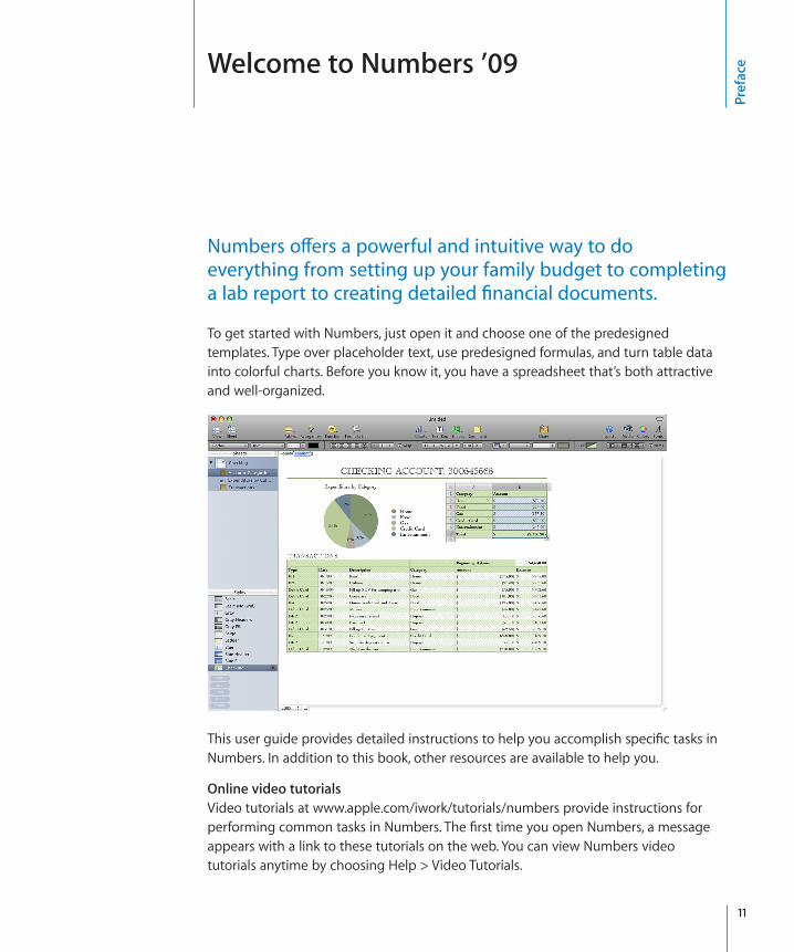
Numbers offers a powerful and intuitive way to do everything from setting up your family budget to completing a lab report to creating detailed financial documents.
To get started with Numbers, just open it and choose one of the predesigned templates. Type over placeholder text, use predesigned formulas, and turn table data into colorful charts. Before you know it, you have a spreadsheet that’s both attractive and well-organized.
This user guide provides detailed instructions to help you accomplish specific tasks in Numbers. In addition to this book, other resources are available to help you.
Online video tutorialsVideo tutorials at www.apple.com/iwork/tutorials/numbers provide instructions for performing common tasks in Numbers. The first time you open Numbers, a message appears with a link to these tutorials on the web. You can view Numbers video tutorials anytime by choosing Help > Video Tutorials.
Pref
aceWelcome to Numbers ’09
12 Preface Welcome to Numbers ’09
Onscreen helpOnscreen help contains detailed instructions for completing all Numbers tasks. To open help, open Numbers and choose Help > Numbers Help. The first page of help also provides access to useful websites.
iWork Formulas and Functions Help and user guideiWork Formulas and Functions Help and the iWork Formulas and Functions User Guide contain detailed instructions for using formulas and powerful functions in your spreadsheets. To open the user guide, choose Help > “iWork Formulas and Functions User Guide.” To open help, choose Help > “iWork Formulas and Functions Help.”
iWork websiteRead the latest news and information about iWork at www.apple.com/iwork.
Support websiteFind detailed information about solving problems at www.apple.com/support/numbers.
Help tagsNumbers provides help tags—brief text descriptions—for most onscreen items. To see a help tag, hold the pointer over an item for a few seconds.
13
This chapter introduces you to the windows and tools you use to work on Numbers spreadsheets.
When you create a Numbers spreadsheet, you first select a template to start from.
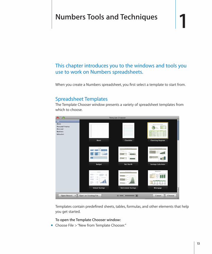
Spreadsheet TemplatesThe Template Chooser window presents a variety of spreadsheet templates from which to choose.
Templates contain predefined sheets, tables, formulas, and other elements that help you get started.
To open the Template Chooser window:�Choose File > “New from Template Chooser.” m
1Numbers Tools and Techniques
Here are ways to use the Template Chooser window:�To view thumbnails of all the templates, click All in the list of template categories on m
the left side of the Template Chooser window.
To view templates by category, click Blank, Personal Finance, or another category.
To increase or decrease the size of the thumbnails, drag the slider at the bottom of m
the window.
To create a spreadsheet using a specific template, click the template and then m
click Choose.
If you want to start from a plain spreadsheet, that contains no formatting, select the Blank template.
See “Creating a New Spreadsheet” on page 28, “Importing a Document from Another Application” on page 29, and “Using CSV or OFX Files in a Spreadsheet” on page 30 to learn how to create a Numbers spreadsheet.
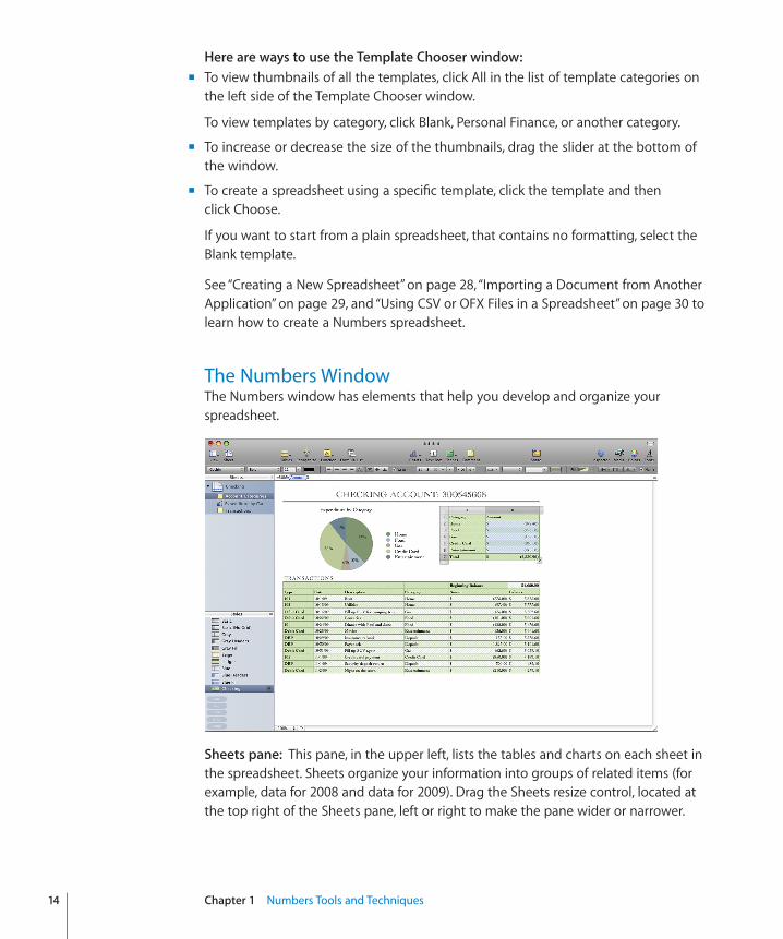
The Numbers WindowThe Numbers window has elements that help you develop and organize your spreadsheet.
Sheets pane:� This pane, in the upper left, lists the tables and charts on each sheet in the spreadsheet. Sheets organize your information into groups of related items (for example, data for 2008 and data for 2009). Drag the Sheets resize control, located at the top right of the Sheets pane, left or right to make the pane wider or narrower.
14 Chapter 1 Numbers Tools and Techniques
Chapter 1 Numbers Tools and Techniques 15
Toolbar:� Located at the top of the window, the toolbar gives you one-click access to commonly used tools. Use it to quickly add a sheet, table, text box, media file, and other objects.
Format bar:� Below the toolbar, the format bar provides convenient access to tools for editing a selected object.
Formula bar:� Below the format bar, the formula bar lets you create and edit formulas or other content in a selected table cell.
Sheet canvas:� The main part of the window, the sheet canvas shows objects on a selected sheet. You can drag tables, charts, and other objects on the sheet canvas to rearrange them.
Styles pane:� Below the Sheets pane, the Styles pane lists table styles predesigned for the template you’re using. Select a table, and click a table style to instantly change the table’s appearance. Drag the Styles resize control, located at the top right of the Styles pane, up or down to enlarge or shrink the pane.
Instant calculation results:� Below the Styles pane is an area that displays the results of calculations for values in selected table cells.
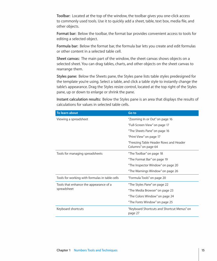
To learn about Go to
Viewing a spreadsheet “Zooming In or Out” on page 16
“Full-Screen View” on page 17
“The Sheets Pane” on page 16
“Print View” on page 17
“Freezing Table Header Rows and Header Columns” on page 64
Tools for managing spreadsheets “The Toolbar” on page 18
“The Format Bar” on page 19
“The Inspector Window” on page 20
“The Warnings Window” on page 26
Tools for working with formulas in table cells “Formula Tools” on page 20
Tools that enhance the appearance of a spreadsheet
“The Styles Pane” on page 22
“The Media Browser” on page 23
“The Colors Window” on page 24
“The Fonts Window” on page 25
Keyboard shortcuts “Keyboard Shortcuts and Shortcut Menus” on page 27
Zooming In or OutYou can enlarge (zoom in) or reduce (zoom out) your view of a sheet.
Here are ways to zoom in or out on a sheet:�Choose View > Zoom > Zoom In or View > Zoom > Zoom Out. m
To return to 100%, choose View > Zoom > Actual Size.
Choose a magnification level from the pop-up menu at the bottom left of the canvas. m
When you view a sheet in Print View, decrease the zoom level to view more pages in the window at one time.
If you’re using Numbers in Mac OS X v10.7 (Lion) or later, you can also view the application window in full-screen view, to help you work without distractions. To learn more, see “Full-Screen View” on page 17.
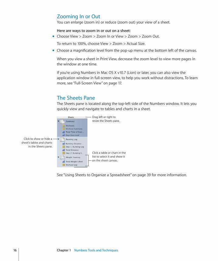
The Sheets PaneThe Sheets pane is located along the top-left side of the Numbers window. It lets you quickly view and navigate to tables and charts in a sheet.
Click to show or hide a sheet’s tables and charts
in the Sheets pane.
Drag left or right to resize the Sheets pane.
Click a table or chart in the list to select it and show it on the sheet canvas.
See “Using Sheets to Organize a Spreadsheet” on page 39 for more information.
16 Chapter 1 Numbers Tools and Techniques
Chapter 1 Numbers Tools and Techniques 17
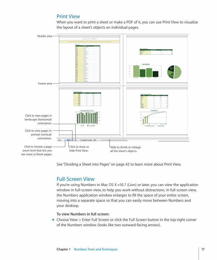
Print ViewWhen you want to print a sheet or make a PDF of it, you can use Print View to visualize the layout of a sheet’s objects on individual pages.
Click to show or hide Print View.
Slide to shrink or enlargeall the sheet’s objects.
Footer area
Header area
Click to choose a page zoom level that lets you
see more or fewer pages.
Click to view pages in portrait (vertical)
orientation.
Click to view pages in landscape (horizontal)
orientation.
See “Dividing a Sheet into Pages” on page 42 to learn more about Print View.
Full-Screen ViewIf you’re using Numbers in Mac OS X v10.7 (Lion) or later, you can view the application window in full-screen view, to help you work without distractions. In full-screen view, the Numbers application window enlarges to fill the space of your entire screen, moving into a separate space so that you can easily move between Numbers and your desktop.
To view Numbers in full screen:�Choose View > Enter Full Screen or click the Full Screen button in the top-right corner m
of the Numbers window (looks like two outward-facing arrows).
To exit full-screen view, do any of the following:�:�Press Escape on your keyboard. m
Move the pointer to the top of the screen to show the menu bar, and then click the m
Full Screen button in the top-right corner of the screen.
Choose View > Exit Full Screen. m
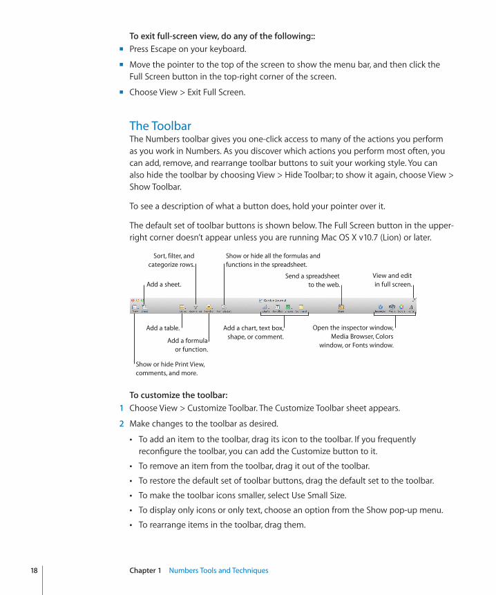
The ToolbarThe Numbers toolbar gives you one-click access to many of the actions you perform as you work in Numbers. As you discover which actions you perform most often, you can add, remove, and rearrange toolbar buttons to suit your working style. You can also hide the toolbar by choosing View > Hide Toolbar; to show it again, choose View > Show Toolbar.
To see a description of what a button does, hold your pointer over it.
The default set of toolbar buttons is shown below. The Full Screen button in the upper-right corner doesn’t appear unless you are running Mac OS X v10.7 (Lion) or later.
Open the inspector window, Media Browser, Colors
window, or Fonts window.
Send a spreadsheet to the web.
Add a chart, text box, shape, or comment.
Add a table.
Add a formula or function.
Sort, filter, and categorize rows.
Add a sheet.
Show or hide Print View, comments, and more.
Show or hide all the formulas and functions in the spreadsheet.
View and edit in full screen.
To customize the toolbar:� 1 Choose View > Customize Toolbar. The Customize Toolbar sheet appears.
2 Make changes to the toolbar as desired.
To add an item to the toolbar, drag its icon to the toolbar. If you frequently Âreconfigure the toolbar, you can add the Customize button to it.
To remove an item from the toolbar, drag it out of the toolbar. Â
To restore the default set of toolbar buttons, drag the default set to the toolbar. Â
To make the toolbar icons smaller, select Use Small Size. Â
To display only icons or only text, choose an option from the Show pop-up menu. Â
To rearrange items in the toolbar, drag them. Â
18 Chapter 1 Numbers Tools and Techniques
Chapter 1 Numbers Tools and Techniques 19
3 Click Done.
You can also customize the toolbar by using these shortcuts:
To remove an item from the toolbar, press the Command key while dragging the Âitem out of the toolbar.
You can also press the Control key while you click the item, and then choose Remove Item from the shortcut menu.
To move an item, press the Command key while dragging the item around in the Âtoolbar.
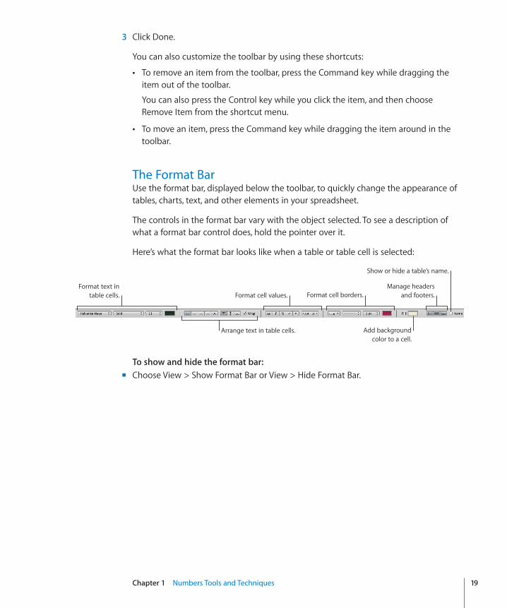
The Format BarUse the format bar, displayed below the toolbar, to quickly change the appearance of tables, charts, text, and other elements in your spreadsheet.
The controls in the format bar vary with the object selected. To see a description of what a format bar control does, hold the pointer over it.
Here’s what the format bar looks like when a table or table cell is selected:
Arrange text in table cells.
Format cell borders.
Add background color to a cell.
Format cell values.Manage headers
and footers.
Show or hide a table’s name.
Format text in table cells.
To show and hide the format bar:�Choose View > Show Format Bar or View > Hide Format Bar. m
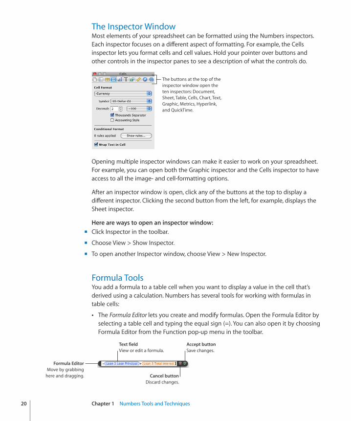
The Inspector WindowMost elements of your spreadsheet can be formatted using the Numbers inspectors. Each inspector focuses on a different aspect of formatting. For example, the Cells inspector lets you format cells and cell values. Hold your pointer over buttons and other controls in the inspector panes to see a description of what the controls do.
The buttons at the top of the inspector window open the ten inspectors: Document, Sheet, Table, Cells, Chart, Text, Graphic, Metrics, Hyperlink, and QuickTime.
Opening multiple inspector windows can make it easier to work on your spreadsheet. For example, you can open both the Graphic inspector and the Cells inspector to have access to all the image- and cell-formatting options.
After an inspector window is open, click any of the buttons at the top to display a different inspector. Clicking the second button from the left, for example, displays the Sheet inspector.
Here are ways to open an inspector window:� Click Inspector in the toolbar. m
Choose View > Show Inspector. m
To open another Inspector window, choose View > New Inspector. m
Formula ToolsYou add a formula to a table cell when you want to display a value in the cell that’s derived using a calculation. Numbers has several tools for working with formulas in table cells:
The  Formula Editor lets you create and modify formulas. Open the Formula Editor by selecting a table cell and typing the equal sign (=). You can also open it by choosing Formula Editor from the Function pop-up menu in the toolbar.
Cancel buttonDiscard changes.
Accept buttonSave changes.
Text fieldView or edit a formula.
Formula EditorMove by grabbing
here and dragging.
20 Chapter 1 Numbers Tools and Techniques
Chapter 1 Numbers Tools and Techniques 21
Learn more about this editor in “Adding and Editing Formulas Using the Formula Editor” on page 122.
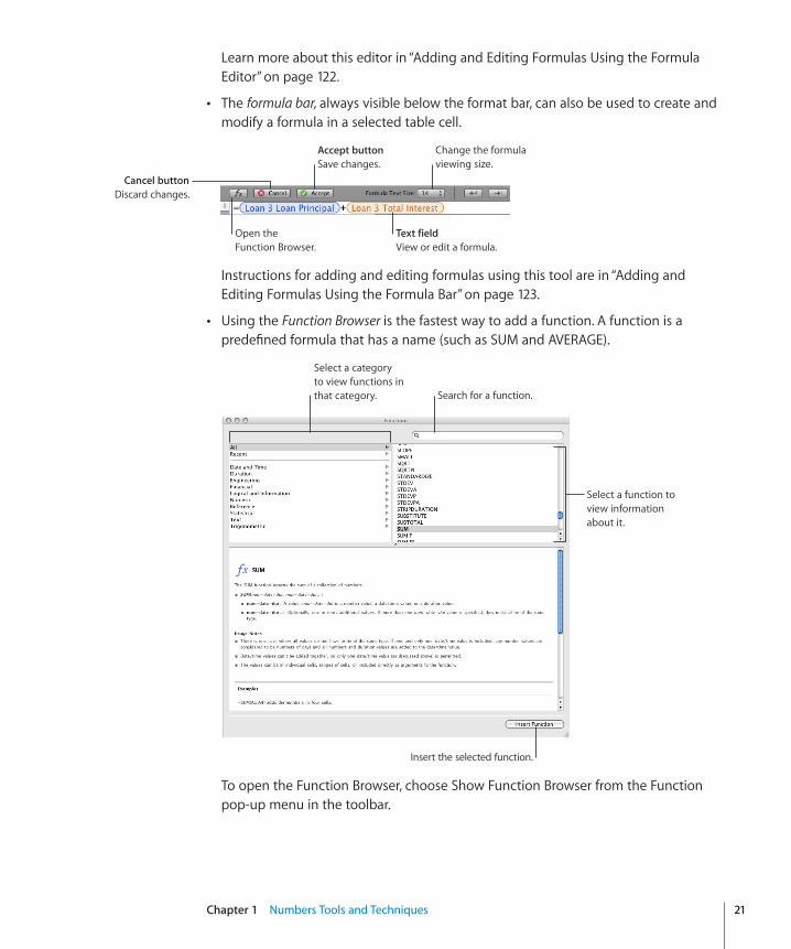
The  formula bar, always visible below the format bar, can also be used to create and modify a formula in a selected table cell.
Open the Function Browser.
Cancel buttonDiscard changes.
Accept buttonSave changes.
Change the formula viewing size.
Text fieldView or edit a formula.
Instructions for adding and editing formulas using this tool are in “Adding and Editing Formulas Using the Formula Bar” on page 123.
Using the  Function Browser is the fastest way to add a function. A function is a predefined formula that has a name (such as SUM and AVERAGE).
Select a function to view information about it.
Search for a function.
Insert the selected function.
Select a category to view functions in that category.
To open the Function Browser, choose Show Function Browser from the Function pop-up menu in the toolbar.
“Adding Functions to Formulas” on page 124 explains how to use the Function Browser. To learn about all the iWork functions, and to review numerous examples that illustrate how to use them, choose Help > “iWork Formulas and Functions Help” or Help > “iWork Formulas and Functions User Guide.”
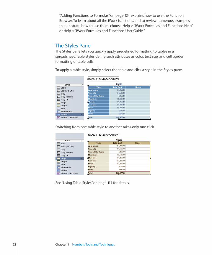
The Styles PaneThe Styles pane lets you quickly apply predefined formatting to tables in a spreadsheet. Table styles define such attributes as color, text size, and cell border formatting of table cells.
To apply a table style, simply select the table and click a style in the Styles pane.
Switching from one table style to another takes only one click.
See “Using Table Styles” on page 114 for details.
22 Chapter 1 Numbers Tools and Techniques
Chapter 1 Numbers Tools and Techniques 23
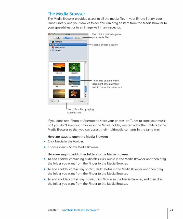
The Media BrowserThe Media Browser provides access to all the media files in your iPhoto library, your iTunes library, and your Movies folder. You can drag an item from the Media Browser to your spreadsheet or to an image well in an inspector.
Second, choose a source.
First, click a button to go to your media files.
Third, drag an item to the document or to an image well in one of the inspectors.
Search for a file by typing its name here.
If you don’t use iPhoto or Aperture to store your photos, or iTunes to store your music, or if you don’t keep your movies in the Movies folder, you can add other folders to the Media Browser so that you can access their multimedia contents in the same way.
Here are ways to open the Media Browser:�Click Media in the toolbar. m
Choose View > Show Media Browser. m
Here are ways to add other folders to the Media Browser:�To add a folder containing audio files, click Audio in the Media Browser, and then drag m
the folder you want from the Finder to the Media Browser.
To add a folder containing photos, click Photos in the Media Browser, and then drag m
the folder you want from the Finder to the Media Browser.
To add a folder containing movies, click Movies in the Media Browser, and then drag m
the folder you want from the Finder to the Media Browser.
To learn how to Go to
Import an image “Working with Images” on page 194
Add a sound file “Adding a Sound File” on page 209
Add a movie file “Adding a Movie File” on page 210
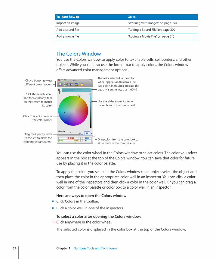
The Colors WindowYou use the Colors window to apply color to text, table cells, cell borders, and other objects. While you can also use the format bar to apply colors, the Colors window offers advanced color management options.
The color selected in the color wheel appears in this box. (The two colors in this box indicate the opacity is set to less than 100%.)
Use the slider to set lighter or darker hues in the color wheel.
Click to select a color in the color wheel.
Drag colors from the color box to store them in the color palette.
Click the search icon, and then click any item on the screen to match
its color.
Click a button to view different color models.
Drag the Opacity slider to the left to make the
color more transparent.
You can use the color wheel in the Colors window to select colors. The color you select appears in the box at the top of the Colors window. You can save that color for future use by placing it in the color palette.
To apply the colors you select in the Colors window to an object, select the object and then place the color in the appropriate color well in an inspector. You can click a color well in one of the inspectors and then click a color in the color well. Or you can drag a color from the color palette or color box to a color well in an inspector.
Here are ways to open the Colors window:�Click Colors in the toolbar. m
Click a color well in one of the inspectors. m
To select a color after opening the Colors window:� 1 Click anywhere in the color wheel.
The selected color is displayed in the color box at the top of the Colors window.
24 Chapter 1 Numbers Tools and Techniques
Chapter 1 Numbers Tools and Techniques 25
2 To make the color lighter or darker, drag the slider on the right side of the Colors window.
3 To make the color more transparent, drag the Opacity slider to the left or enter a percentage value in the Opacity field.
4 To use the color palette, open it by dragging the handle at the bottom of the Colors window.
Save a color in the palette by dragging a color from the color box to the color palette. To remove a color from the palette, drag a blank square to the color you want to remove.
5 To match the color of another item on the screen, click the search icon to the left of the color box in the Colors window.
Click the item on the screen whose color you want to match. The color appears in the color box. Select the item you want to color in the spreadsheet, and then drag the color from the color box to the item.
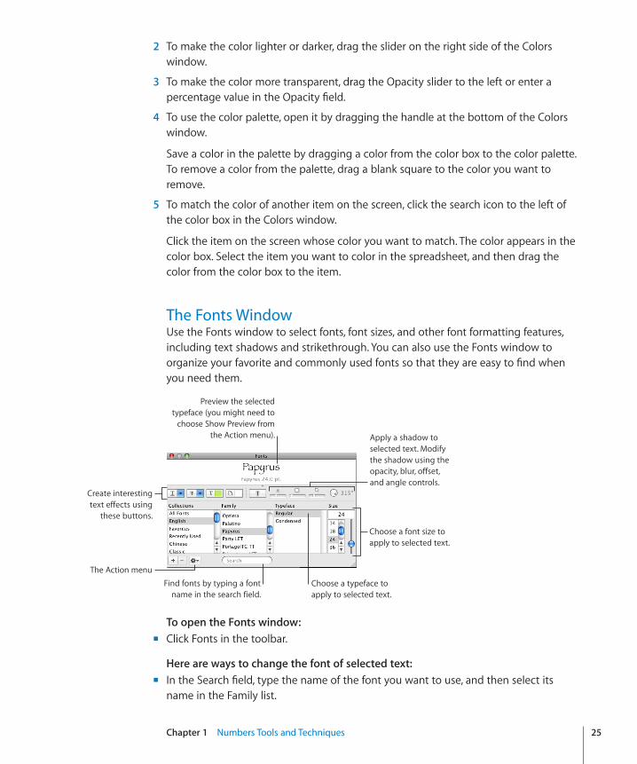
The Fonts WindowUse the Fonts window to select fonts, font sizes, and other font formatting features, including text shadows and strikethrough. You can also use the Fonts window to organize your favorite and commonly used fonts so that they are easy to find when you need them.
Create interesting text effects using
these buttons.
The Action menu
Choose a typeface to apply to selected text.
Find fonts by typing a font name in the search field.
Choose a font size to apply to selected text.
Apply a shadow to selected text. Modify the shadow using the opacity, blur, offset, and angle controls.
Preview the selected typeface (you might need to
choose Show Preview from the Action menu).
To open the Fonts window:�Click Fonts in the toolbar. m
Here are ways to change the font of selected text:�In the Search field, type the name of the font you want to use, and then select its m
name in the Family list.
Select a typeface (for example, Italic or Bold) from the Typeface list. m
In the Size column, type or select the font size you want. m
Here are ways to use the controls at the top of the Fonts window:�Rest your pointer over any control along the top of the window to view a help tag describing what each control does. If you don’t see the controls, choose Show Effects from the Action pop-up menu (looks like a gear) in the lower-left corner of the window.
To underline text, choose an underline style (such as single or double) from the Text m
Underline pop-up menu.
To apply a strikethrough style (such as single or double), choose a style from the Text m
Strikethrough pop-up menu.
To apply color to text, click the Text Color button to open the Colors window. See “ m The Colors Window” on page 24 for details.
To apply color behind a paragraph, click the Document Color button to open the m
Colors window.
To apply a shadow, click the Text Shadow button. Use the Shadow Opacity, Shadow m
Blur, Shadow Offset, and Shadow Angle controls to format the shadow.
To organize fonts:� 1 Click the Add Collection (+) button to create and name a new collection.
2 Select some text and format it with the font family, typeface, and size that you want.
3 Drag the font name from the Family list to the collection where you want to file it.
To set up the Fonts window for frequent use:�Leave the Fonts window open as you work. Resize the window using the control in the m
bottom-right corner of the window so that only the font families and typefaces in your selected font collection are visible.
The Warnings WindowWhen you import a document into Numbers, or export a Numbers spreadsheet to another format, some elements might not transfer as expected. The Document Warnings window lists any problems encountered.
If there are problems, you’ll see a message enabling you to review the warnings. If you choose not to review them, you can see the Warnings window at any time by choosing View > Show Document Warnings.
If you see a warning about a missing font, you can select the warning and click Replace Font to choose a replacement font.
26 Chapter 1 Numbers Tools and Techniques
Chapter 1 Numbers Tools and Techniques 27
You can copy one or more warnings by selecting them in the Document Warnings window and choosing Edit > Copy. You can then paste the copied text into an email message, text file, or some other window.
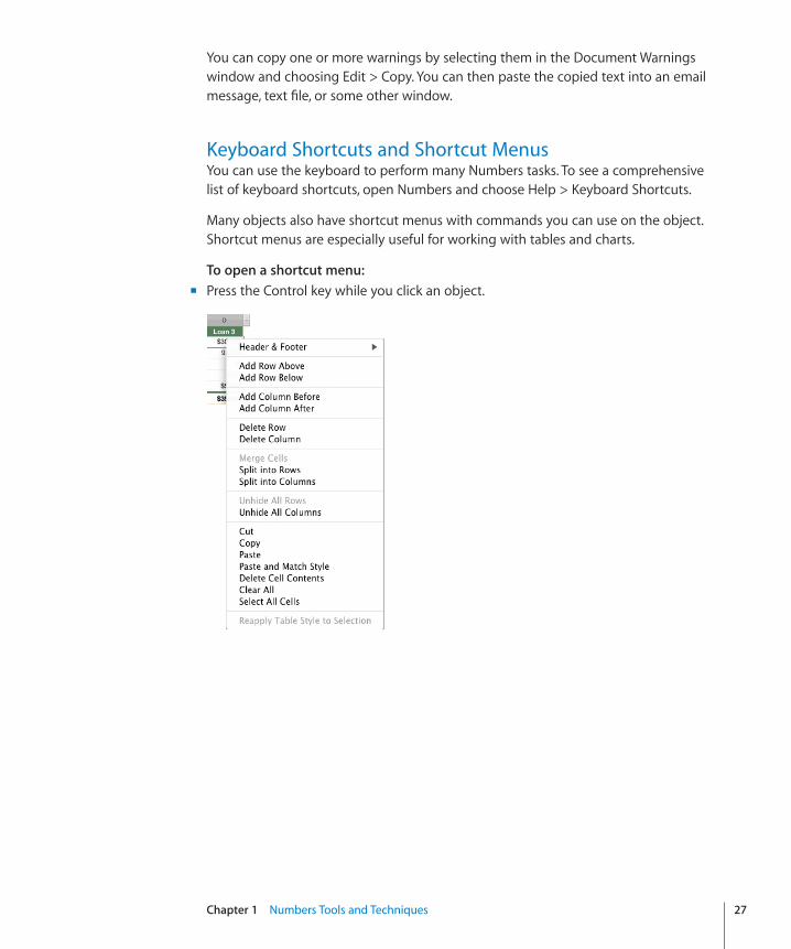
Keyboard Shortcuts and Shortcut MenusYou can use the keyboard to perform many Numbers tasks. To see a comprehensive list of keyboard shortcuts, open Numbers and choose Help > Keyboard Shortcuts.
Many objects also have shortcut menus with commands you can use on the object. Shortcut menus are especially useful for working with tables and charts.
To open a shortcut menu:�Press the Control key while you click an object. m
28
This chapter describes how to manage Numbers spreadsheets.
You can create a Numbers spreadsheet by opening Numbers and choosing a template. You can also import a document created in another application, such as Microsoft Excel or AppleWorks 6, or create a spreadsheet using a CSV (comma-separated value) file.
This chapter explains how to create new Numbers spreadsheets, as well as how to open existing spreadsheets and save spreadsheets.
This chapter also provides instructions for organizing spreadsheets into sheets and for organizing them into pages when you print them or create PDFs.
Creating a New SpreadsheetTo create a new Numbers spreadsheet, you pick the template that provides appropriate formatting and content characteristics.
Start with the Blank template to build your spreadsheet from scratch. Or select one of the many other templates to get a head start creating a budget, planning a party, and more using predefined tables, charts, and sample data.
To create a new spreadsheet:� 1 Open Numbers by clicking its icon in the Dock or by double-clicking its icon in
the Finder.
If Numbers is open, choose File > “New from Template Chooser.”
2Creating, Saving, and Organizing a Numbers Spreadsheet
Chapter 2 Creating, Saving, and Organizing a Numbers Spreadsheet 29
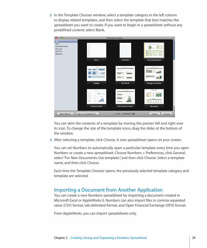
2 In the Template Chooser window, select a template category in the left column to display related templates, and then select the template that best matches the spreadsheet you want to create. If you want to begin in a spreadsheet without any predefined content, select Blank.
You can skim the contents of a template by moving the pointer left and right over its icon. To change the size of the template icons, drag the slider at the bottom of the window.
3 After selecting a template, click Choose. A new spreadsheet opens on your screen.
You can set Numbers to automatically open a particular template every time you open Numbers or create a new spreadsheet. Choose Numbers > Preferences, click General, select “For New Documents: Use template:”, and then click Choose. Select a template name, and then click Choose.
Each time the Template Chooser opens, the previously selected template category and template are selected.
Importing a Document from Another ApplicationYou can create a new Numbers spreadsheet by importing a document created in Microsoft Excel or AppleWorks 6. Numbers can also import files in comma-separated value (CSV) format, tab-delimited format, and Open Financial Exchange (OFX) format.
From AppleWorks, you can import spreadsheets only.
Here are ways to import a document:�Drag the document to the Numbers application icon. A new Numbers spreadsheet m
opens, and the contents of the imported document are displayed.
In Numbers, choose File > Open, select the document, and then click Open. m
You can import Address Book data to quickly create tables that contain names, phone m
numbers, addresses, and other information for your contacts. See “Using Address Book Fields” on page 231 for instructions.
If you want to import CSV or OFX data, see “ m Using CSV or OFX Files in a Spreadsheet” on page 30.
If you can’t import a document, try opening the document in another application and saving it in a format Numbers can read, or copy and paste the contents into an existing Numbers spreadsheet.
You can also export Numbers spreadsheets to Microsoft Excel, PDF, and CSV files. See “Exporting a Spreadsheet to Other Document Formats” on page 237 for details.
Using CSV or OFX Files in a SpreadsheetTo add CSV or OFX data to an open spreadsheet:�
1 Select a sheet.
2 Do one of the following:
To create one or more new tables, drag a CSV or OFX file from the Finder onto the Âsheet’s canvas.
To add CSV or OFX data to an empty table, drag the CSV or OFX file onto the table. Â
The data is added; additional columns are created if necessary.
To add CSV or OFX data to a table that contains data, drag the CSV or OFX file onto Âthe table.
If the columns don’t match, choose an option from the sheet that appears. You can cancel the import, add columns to the table, ignore extra columns, or create a new table from the CSV or OFX data.
Opening an Existing SpreadsheetYou can open an iWork ’08 or iWork ’09 spreadsheet. To take advantage of new features, save iWork ’08 spreadsheets in iWork ’09 format. To let iWork ’08 users access your spreadsheet, save it in iWork ’08 format.
When you open an iWork ’09 spreadsheet that’s password-protected, you need to type the password in the Password field before you can view the spreadsheet contents.
30 Chapter 2 Creating, Saving, and Organizing a Numbers Spreadsheet
Chapter 2 Creating, Saving, and Organizing a Numbers Spreadsheet 31
Here are ways to open an existing spreadsheet:�To open a spreadsheet from the Template Chooser, click “Open an Existing File” in the m
Template Chooser window, select the document, and then click Open.
To open a spreadsheet you’ve worked with recently, choose it from the Open Recent pop-up menu at the bottom left of the Template Chooser window.
To open a spreadsheet when you’re working in one, choose File > Open, select the m
spreadsheet, and then click Open.
To open a spreadsheet you’ve worked with recently, choose File > Open Recent and choose the spreadsheet from the submenu.
To open a Numbers spreadsheet from the Finder, double-click the spreadsheet icon or m
drag it to the Numbers application icon.
If you see a message that a font or file is missing when you open a spreadsheet, you can still use the spreadsheet. Numbers lets you choose fonts to substitute for missing fonts. Or you can add missing fonts by quitting Numbers and adding the fonts to your Fonts folder (for more information, see Mac Help). To make missing movies or sound files reappear, add them to the spreadsheet again.
Password-Protecting a SpreadsheetWhen you want to restrict access to a Numbers document, you can assign it a password. Passwords can consist of almost any combination of numerals and capital or lowercase letters and several of the special keyboard characters. Passwords with combinations of letters, numbers, and other characters are generally considered more secure.
When you save a spreadsheet in iWork ’08 or Excel format, you can’t use password protection, but when you export a spreadsheet as a PDF you can assign a password to it.
Here are ways to manage password-protection in a Numbers spreadsheet:�To use a password-protected spreadsheet, open the spreadsheet, type the password m
when prompted, optionally select “Remember this password in my keychain,” and then click OK.
If you incorrectly type the password twice, any hint defined when the password was created is displayed.
To add a password to the spreadsheet, open the Document inspector and select m
“Require password to open” in the Document pane. Type the password you want to use in the fields provided, and then click Set Password. A lock icon appears next to the document title to indicate that your document is password protected.
If you want help to create an unusual or strong password, click the button with the key-shaped icon next to the Password field to open the Password Assistant and use it to help you create a password. You can select a type of password in the pop-up menu, depending on which password characteristics are most important to you.
A password appears in the Suggestion field; its strength (“stronger” passwords are more difficult to break) is indicated by the length and green color of the Quality bar. If you like the suggested password, copy it and paste it into the Password field.
If you don’t like the suggested password, you can choose a different password from the Suggestion field pop-up menu, increase the password length by dragging the slider, or type your own.
To remove a password from a spreadsheet, open your password-protected document, m
and then deselect “Require password to open” in the Document inspector’s Document pane. Type the document password to disable password protection and click OK.
To change a password, open the Document inspector, click Change Password, enter m
your information, and then click Change Password.
To add a password for a PDF of your spreadsheet, follow the instructions in “ m Exporting a Spreadsheet in PDF Format” on page 237.
Saving a SpreadsheetIf you’re running Mac OS X v10.7 (Lion) or later, Numbers auto-saves your spreadsheet frequently in the background, so that you don’t have to worry about losing changes you made if the application closes unexpectedly. You can also save the spreadsheet manually, creating an archive of older versions, which can be recovered at any time.
No matter which operating system you’re running, it’s a good idea to save your spreadsheet often as you work. After you save it for the first time, you can press Command-S to resave it using the same settings.
When you save a Numbers spreadsheet, fonts are not included as part of the spreadsheet. If you transfer a Numbers spreadsheet to another computer, make sure the fonts used in the spreadsheet have been installed in the Fonts folder of that computer.
To save a spreadsheet for the first time: 1 Choose File > Save, or press Command-S.
2 In the Save As field, type a name for the spreadsheet.
3 Choose where you want to save the spreadsheet.
If the directory in which you want to save the spreadsheet isn’t visible in the Where pop-up menu, click the disclosure triangle to the right of the Save As field and navigate to a different location.
32 Chapter 2 Creating, Saving, and Organizing a Numbers Spreadsheet
Chapter 2 Creating, Saving, and Organizing a Numbers Spreadsheet 33
4 If you want the spreadsheet to display a Quick Look in the Finder in Mac OS X version 10.5 or later, select “Include preview in document.”
If you always want to include a preview in your spreadsheets, choose Numbers > Preferences, click General, and select “Include preview in document by default.”
5 If you want to save the spreadsheet as an iWork ’08 or Excel spreadsheet, select “Save copy as” and choose iWork ’08 or Excel Document from the pop-up menu.
6 If you or someone else will open the spreadsheet on another computer, click Advanced Options and set up options that determine what’s copied into your spreadsheet.
Copy audio and movies into document:� If you use movies or sound files in your spreadsheet, selecting this checkbox saves the movie or sound files with the spreadsheet so the files play if the spreadsheet is opened on another computer. You can deselect this checkbox so that the file size is smaller, but the media files won’t play on other computers. See “Reducing Image File Sizes” on page 198 and “Reducing the Size of Media Files” on page 212 to learn other techniques for reducing file size.
Copy template images into document:� If you don’t select this option and you open the spreadsheet on a computer that doesn’t have Numbers installed, the spreadsheet might look different.
7 Click Save.
In general, you can save Numbers spreadsheets only to computers and servers that use Mac OS X. Numbers is not compatible with Mac OS 9 computers and Windows servers running Services for Macintosh. If you must save to a Windows computer, try using AFP server software available for Windows to do so.
To learn how to Go to
Share your spreadsheets with others “Printing a Spreadsheet” on page 236
“Sending Your Numbers Spreadsheet to iWork.com public beta” on page 239
“Exporting a Spreadsheet to Other Document Formats” on page 237
“Sending a Spreadsheet Using Email” on page 242
“Sending a Spreadsheet to iWeb” on page 242
Undo or prevent changes made to a spreadsheet “Undoing Changes” on page 34
“Locking a Spreadsheet So It Can’t Be Edited” on page 34
Save different versions of a spreadsheet “Automatically Saving a Backup Version” on page 35
“Finding an Archived Version of a Spreadsheet” on page 36
“Saving a Copy of a Spreadsheet” on page 36
“Saving a Spreadsheet as a Template” on page 38
Save terms that Spotlight can use to locate a spreadsheet
“Saving Spotlight Search Terms for a Spreadsheet” on page 38
Close a spreadsheet without quitting “Closing a Spreadsheet Without Quitting Numbers” on page 39
Undoing ChangesIf you don’t want to save changes you made to your spreadsheet since opening it or last saving it, you can undo them.
Here are ways to undo changes:�To undo your most recent change, choose Edit > Undo. m
To undo multiple changes, choose Edit > Undo multiple times. You can undo any m
changes you made since opening the spreadsheet or reverting to the last saved version.
To restore changes you’ve undone using Edit > Undo, choose Edit > Redo one or m
more times.
To undo all changes you made since the last time you saved your spreadsheet, choose m
File > “Revert to Saved” and then click Revert.
Locking a Spreadsheet So It Can’t Be EditedIf you’re running Mac OS X v10.7 (Lion) or later, you can lock your spreadsheet so you can’t edit it by accident, when you only intend to open and view it. You can easily unlock the spreadsheet at any time to continue editing it.
34 Chapter 2 Creating, Saving, and Organizing a Numbers Spreadsheet
Chapter 2 Creating, Saving, and Organizing a Numbers Spreadsheet 35
To lock a spreadsheet:� 1 Open the spreadsheet you want to lock, and hold your pointer over the name of the
spreadsheet at the top of the Numbers application window.
A triangle appears.
2 Click the triangle and choose Lock from the pop-up menu.
To unlock a spreadsheet for editing:�Hold your pointer over the name of the spreadsheet at the top of the Numbers m
application window until the triangle appears, click the triangle, and then choose Unlock.
Automatically Saving a Backup VersionEach time you save a spreadsheet, you can save a copy without the changes you made since last saving it. That way, if you change your mind about edits you made, you can go back to (revert to) the backup version of the spreadsheet.
The best way to create backup versions is different, depending upon which version of Mac OS X you’re running. Mac OS X v10.7 (Lion) and later automatically saves a snapshot of your spreadsheet every time you save. You can access an archive of all previous saved versions at any time. To learn about accessing and using past document versions in Lion, see “Finding an Archived Version of a Spreadsheet” on page 36.
If you’re running Mac OS X v10.6.x (Snow Leopard) or earlier, you can set up Numbers to automatically create a copy of the last saved version of your spreadsheet. You may also find this useful if you’re running Lion, and you want to save a backup version of your spreadsheet on another hard disk on your network.
To create an archive of previously saved versions of your spreadsheet on Lion or laterChoose File > “Save a Version,” or press Command-S. m
To create a copy of the last saved version of your spreadsheet:�Choose Numbers > Preferences, click General, and then select “Back up previous version.” m
The next time you save your spreadsheet, a backup version is created in the same location, with “Backup of” preceding the filename. Only one version—the last saved version—is backed up. Every time you save the spreadsheet, the old backup file is replaced with the new backup file.
To revert to the last saved version after making unsaved changes, choose File > “Revert to Saved.” The changes in your open spreadsheet are undone.
Saving a Copy of a SpreadsheetIf you want to duplicate your open spreadsheet, you can save it using a different name or location.
To save a copy of a spreadsheet in Mac OS X v10.7 (Lion) or later:� 1 Choose File > Duplicate.
An untitled copy of the spreadsheet is created. Both copies remain open on your desktop for you to view or edit.
2 Close the window of the untitled copy, type the spreadsheet’s name, and then choose a location from the pop-up menu.
3 Click Save.
To save a copy of a spreadsheet in Mac OS X v10.6.x (Snow Leopard) or earlier:�Choose File > Save As and specify a name and location. m
The spreadsheet with the new name remains open. To work with the previous version, choose File > Open Recent and choose the previous version from the submenu.
You can also automate creating a backup version of the spreadsheet every time you save, retaining the name and location of the original, but with the words “Backup of” preceding the filename. See “Automatically Saving a Backup Version” on page 35.
Finding an Archived Version of a SpreadsheetIf you saved your spreadsheet multiple times on Mac OS X v10.7 (Lion) or later, all the saved versions are automatically archived. You can browse the archive to identify any earlier version that you want to restore or reference. After you identify the archived version that you want, you can restore it as a fully editable copy, or you can just extract from it any text, images, or document settings that you want to use again.
To browse and restore archived versions of your spreadsheet:� 1 Open the spreadsheet for which you want to access older versions, and hold your pointer
over the name of the spreadsheet at the top of the Numbers application window.
A triangle appears.
2 Click the triangle and choose Browse All Versions.
36 Chapter 2 Creating, Saving, and Organizing a Numbers Spreadsheet
Chapter 2 Creating, Saving, and Organizing a Numbers Spreadsheet 37
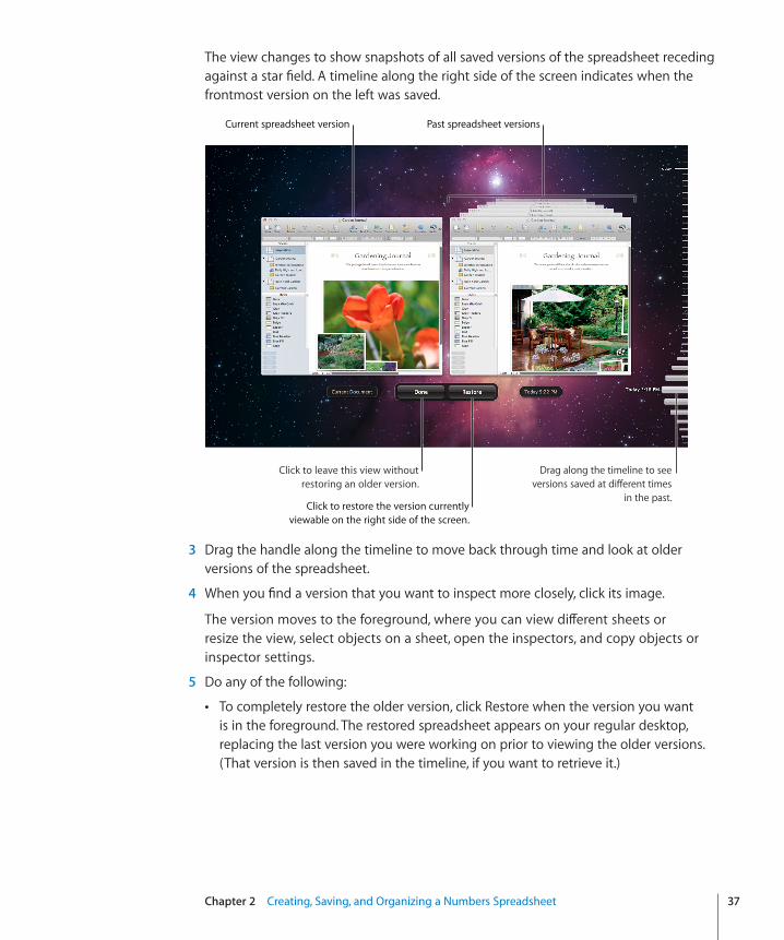
The view changes to show snapshots of all saved versions of the spreadsheet receding against a star field. A timeline along the right side of the screen indicates when the frontmost version on the left was saved.
Past spreadsheet versionsCurrent spreadsheet version
Click to restore the version currently viewable on the right side of the screen.
Click to leave this view without restoring an older version.
Drag along the timeline to see versions saved at different times
in the past.
3 Drag the handle along the timeline to move back through time and look at older versions of the spreadsheet.
4 When you find a version that you want to inspect more closely, click its image.
The version moves to the foreground, where you can view different sheets or resize the view, select objects on a sheet, open the inspectors, and copy objects or inspector settings.
5 Do any of the following:
To completely restore the older version, click Restore when the version you want Âis in the foreground. The restored spreadsheet appears on your regular desktop, replacing the last version you were working on prior to viewing the older versions. (That version is then saved in the timeline, if you want to retrieve it.)
To restore only an object or inspector setting from the older version, copy the Âobject or setting by selecting it and pressing Command-C, and then click Current Document to view the current version of the spreadsheet. Locate the sheet where you want to paste the item you just copied and click to insert the cursor where you want the item to appear on the sheet. Paste the item by pressing Command-V.
To compare the older version side-by-side with the current version, click ÂCurrent Document.
6 To return to your regular desktop, click Done.
Saving a Spreadsheet as a TemplateTo use a spreadsheet you’ve created as a starting point for future documents, you can save the spreadsheet as a template. When you save a spreadsheet as a template, it appears in the Template Chooser.
To save a spreadsheet as a template:�Choose File > “Save as Template.” m
See “Designing a Template” on page 244 for additional details.
Saving Spotlight Search Terms for a SpreadsheetYou can store such information as author name and keywords in Numbers spreadsheets, and then use Spotlight to locate spreadsheets containing that information.
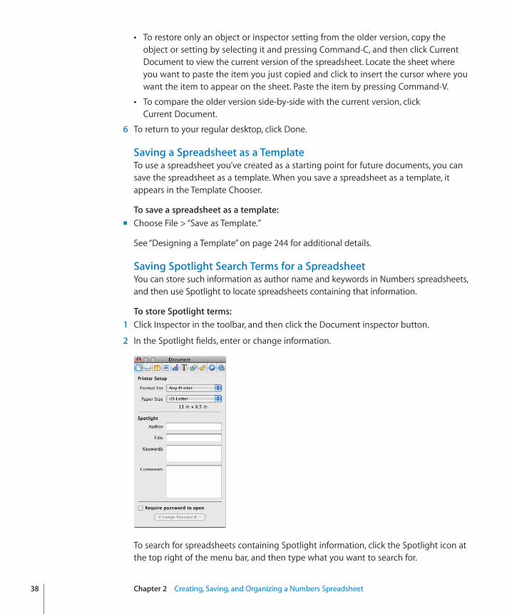
To store Spotlight terms:� 1 Click Inspector in the toolbar, and then click the Document inspector button.
2 In the Spotlight fields, enter or change information.
To search for spreadsheets containing Spotlight information, click the Spotlight icon at the top right of the menu bar, and then type what you want to search for.
38 Chapter 2 Creating, Saving, and Organizing a Numbers Spreadsheet
Chapter 2 Creating, Saving, and Organizing a Numbers Spreadsheet 39
Closing a Spreadsheet Without Quitting NumbersWhen you have finished working with a spreadsheet, you can close it without quitting Numbers.
Here are ways to close the active spreadsheet and keep the application open:�To close the active spreadsheet, choose File > Close or click the close button in the m
upper-left corner of the Numbers window.
To close all open spreadsheets, press the Option key and choose File > Close All or m
click the active spreadsheet’s close button.
If you’ve made changes since you last saved the spreadsheet, Numbers prompts you to save.
Using Sheets to Organize a SpreadsheetLike chapters in a book, sheets let you divide information into manageable groups. For example, you might want to place charts in the same sheet as the tables whose data they display. Or you may want to place all the tables on one sheet and all the charts on another sheet. You might want to use one sheet for keeping track of business contacts and other sheets for friends and relatives.
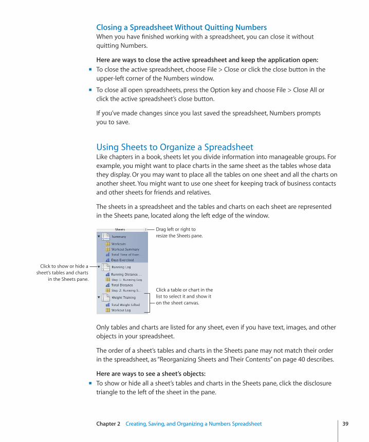
The sheets in a spreadsheet and the tables and charts on each sheet are represented in the Sheets pane, located along the left edge of the window.
Click to show or hide a sheet’s tables and charts
in the Sheets pane.
Drag left or right to resize the Sheets pane.
Click a table or chart in the list to select it and show it on the sheet canvas.
Only tables and charts are listed for any sheet, even if you have text, images, and other objects in your spreadsheet.
The order of a sheet’s tables and charts in the Sheets pane may not match their order in the spreadsheet, as “Reorganizing Sheets and Their Contents” on page 40 describes.
Here are ways to see a sheet’s objects:� To show or hide all a sheet’s tables and charts in the Sheets pane, click the disclosure m
triangle to the left of the sheet in the pane.
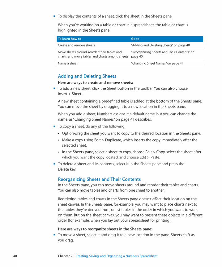
To display the contents of a sheet, click the sheet in the Sheets pane. m
When you’re working on a table or chart in a spreadsheet, the table or chart is highlighted in the Sheets pane.
To learn how to Go to
Create and remove sheets “Adding and Deleting Sheets” on page 40
Move sheets around, reorder their tables and charts, and move tables and charts among sheets
“Reorganizing Sheets and Their Contents” on page 40
Name a sheet “Changing Sheet Names” on page 41
Adding and Deleting SheetsHere are ways to create and remove sheets:� To add a new sheet, click the Sheet button in the toolbar. You can also choose m
Insert > Sheet.
A new sheet containing a predefined table is added at the bottom of the Sheets pane. You can move the sheet by dragging it to a new location in the Sheets pane.
When you add a sheet, Numbers assigns it a default name, but you can change the name, as “Changing Sheet Names” on page 41 describes.
To copy a sheet, do any of the following: m
Option-drag the sheet you want to copy to the desired location in the Sheets pane. Â
Make a copy using Edit > Duplicate, which inserts the copy immediately after the Âselected sheet.
In the Sheets pane, select a sheet to copy, choose Edit > Copy, select the sheet after Âwhich you want the copy located, and choose Edit > Paste.
To delete a sheet and its contents, select it in the Sheets pane and press the m
Delete key.
Reorganizing Sheets and Their ContentsIn the Sheets pane, you can move sheets around and reorder their tables and charts. You can also move tables and charts from one sheet to another.
Reordering tables and charts in the Sheets pane doesn’t affect their location on the sheet canvas. In the Sheets pane, for example, you may want to place charts next to the tables they’re derived from, or list tables in the order in which you want to work on them. But on the sheet canvas, you may want to present these objects in a different order (for example, when you lay out your spreadsheet for printing).
Here are ways to reorganize sheets in the Sheets pane:�To move a sheet, select it and drag it to a new location in the pane. Sheets shift as m
you drag.
40 Chapter 2 Creating, Saving, and Organizing a Numbers Spreadsheet
Chapter 2 Creating, Saving, and Organizing a Numbers Spreadsheet 41
You can also select multiple sheets and move them as a group.
To copy (or cut) and paste sheets, select the sheets, choose Edit > Cut or Edit > Copy, m
select the sheet after which you want to place the sheets you’re moving, and choose Edit > Paste.
To move one or more tables and charts associated with a sheet, select them and drag m
them to a new location in the same sheet or to a different sheet.
You can also use cut/paste or copy/paste actions to move tables and charts in the pane.
To move an object within a sheet in the spreadsheet, select it and drag it to a different location, or use cut/paste or copy/paste actions. To place objects on specific pages for printing or creating a PDF, follow the instructions in “Dividing a Sheet into Pages” on page 42.
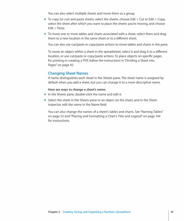
Changing Sheet NamesA name distinguishes each sheet in the Sheets pane. The sheet name is assigned by default when you add a sheet, but you can change it to a more descriptive name.
Here are ways to change a sheet’s name:�In the Sheets pane, double-click the name and edit it. m
Select the sheet in the Sheets pane or an object on the sheet, and in the Sheet m
inspector, edit the name in the Name field.
You can also change the names of a sheet’s tables and charts. See “Naming Tables” on page 52 and “Placing and Formatting a Chart’s Title and Legend” on page 144 for instructions.
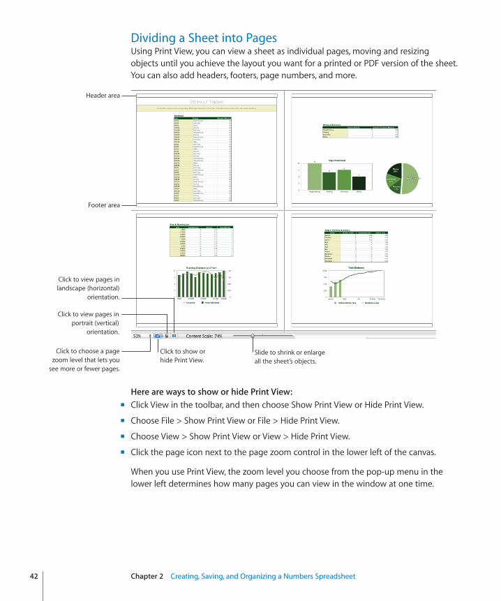
Dividing a Sheet into PagesUsing Print View, you can view a sheet as individual pages, moving and resizing objects until you achieve the layout you want for a printed or PDF version of the sheet. You can also add headers, footers, page numbers, and more.
Click to show or hide Print View.
Slide to shrink or enlargeall the sheet’s objects.
Footer area
Header area
Click to choose a page zoom level that lets you
see more or fewer pages.
Click to view pages in portrait (vertical)
orientation.
Click to view pages in landscape (horizontal)
orientation.
Here are ways to show or hide Print View:�Click View in the toolbar, and then choose Show Print View or Hide Print View. m
Choose File > Show Print View or File > Hide Print View. m
Choose View > Show Print View or View > Hide Print View. m
Click the page icon next to the page zoom control in the lower left of the canvas. m
When you use Print View, the zoom level you choose from the pop-up menu in the lower left determines how many pages you can view in the window at one time.
42 Chapter 2 Creating, Saving, and Organizing a Numbers Spreadsheet
Chapter 2 Creating, Saving, and Organizing a Numbers Spreadsheet 43
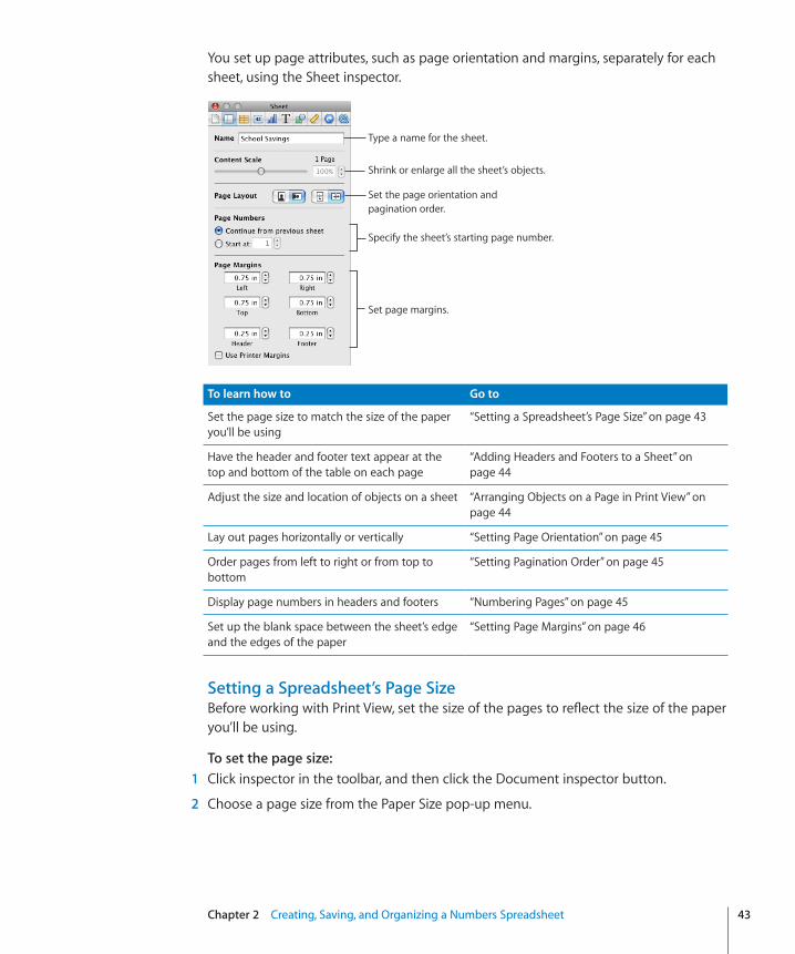
You set up page attributes, such as page orientation and margins, separately for each sheet, using the Sheet inspector.
Type a name for the sheet.
Shrink or enlarge all the sheet’s objects.
Set the page orientation and pagination order.
Set page margins.
Specify the sheet’s starting page number.
To learn how to Go to
Set the page size to match the size of the paper you’ll be using
“Setting a Spreadsheet’s Page Size” on page 43
Have the header and footer text appear at the top and bottom of the table on each page
“Adding Headers and Footers to a Sheet” on page 44
Adjust the size and location of objects on a sheet “Arranging Objects on a Page in Print View” on page 44
Lay out pages horizontally or vertically “Setting Page Orientation” on page 45
Order pages from left to right or from top to bottom
“Setting Pagination Order” on page 45
Display page numbers in headers and footers “Numbering Pages” on page 45
Set up the blank space between the sheet’s edge and the edges of the paper
“Setting Page Margins” on page 46
Setting a Spreadsheet’s Page SizeBefore working with Print View, set the size of the pages to reflect the size of the paper you’ll be using.
To set the page size:� 1 Click inspector in the toolbar, and then click the Document inspector button.
2 Choose a page size from the Paper Size pop-up menu.
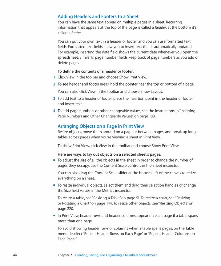
Adding Headers and Footers to a SheetYou can have the same text appear on multiple pages in a sheet. Recurring information that appears at the top of the page is called a header; at the bottom it’s called a footer.
You can put your own text in a header or footer, and you can use formatted text fields. Formatted text fields allow you to insert text that is automatically updated. For example, inserting the date field shows the current date whenever you open the spreadsheet. Similarly, page number fields keep track of page numbers as you add or delete pages.
To define the contents of a header or footer: 1 Click View in the toolbar and choose Show Print View.
2 To see header and footer areas, hold the pointer near the top or bottom of a page.
You can also click View in the toolbar and choose Show Layout.
3 To add text to a header or footer, place the insertion point in the header or footer and insert text.
4 To add page numbers or other changeable values, see the instructions in “Inserting Page Numbers and Other Changeable Values” on page 188.
Arranging Objects on a Page in Print ViewResize objects, move them around on a page or between pages, and break up long tables across pages when you’re viewing a sheet in Print View.
To show Print View, click View in the toolbar and choose Show Print View.
Here are ways to lay out objects on a selected sheet’s pages:�To adjust the size of all the objects in the sheet in order to change the number of m
pages they occupy, use the Content Scale controls in the Sheet inspector.
You can also drag the Content Scale slider at the bottom left of the canvas to resize everything on a sheet.
To resize individual objects, select them and drag their selection handles or change m
the Size field values in the Metrics inspector.
To resize a table, see “Resizing a Table” on page 51. To resize a chart, see “Resizing or Rotating a Chart” on page 144. To resize other objects, see “Resizing Objects” on page 220.
In Print View, header rows and header columns appear on each page if a table spans m
more than one page.
To avoid showing header rows or columns when a table spans pages, on the Table menu deselect “Repeat Header Rows on Each Page” or “Repeat Header Columns on Each Page.”
44 Chapter 2 Creating, Saving, and Organizing a Numbers Spreadsheet
Chapter 2 Creating, Saving, and Organizing a Numbers Spreadsheet 45
Move objects from page to page by dragging them or by cutting and pasting them. m
Setting Page OrientationYou can lay out pages in a sheet in a vertical orientation (portrait) or a horizontal orientation (landscape).
To set a sheet’s page orientation:� 1 Click View in the toolbar and choose Show Print View.
2 Click Inspector in the toolbar, click the Sheet inspector button, and click the appropriate page orientation button in the Page Layout area of the pane.
You can also click a page orientation button at the bottom left of the canvas.
Setting Pagination OrderIn Print View, pages can be ordered from left to right or from top to bottom. This order determines how the document prints and exports to PDF.
To set pagination order:�Click Inspector in the toolbar, click the Sheet inspector button, and then click the top- m
to-bottom or left-to-right button in the Page Layout area of the pane.
Numbering PagesYou can display page numbers in a page’s header or footer.
To number a sheet’s pages:� 1 Select the sheet.
2 Click View in the toolbar and choose Show Print View.
3 Click View in the toolbar and choose Show Layout so you can see the headers and footers.
You can also see the headers and footers by holding the pointer over the top or bottom of a page.
4 Click into the first header or footer to add a page number, following the instructions in “Inserting Page Numbers and Other Changeable Values” on page 188.
5 Click Inspector in the toolbar, click the Sheet inspector button, and then specify the starting page number.
To continue page numbers from the previously selected sheet, select “Continue from previous sheet.”
To start the sheet’s page numbers at a particular number, use the Start At field.
Setting Page MarginsIn Print View, every sheet’s page has margins (blank space between the sheet’s edge and the edges of the paper). These margins are indicated onscreen by light gray lines, visible when you use layout view.
To set the page margins for a sheet:� 1 Select the sheet in the Sheets pane.
2 Click View in the toolbar and choose Show Print View, and then click View in the toolbar and choose Show Layout.
3 Click Inspector in the toolbar, and then click the Sheet inspector button.
4 To set the distance between the layout margins and the left, right, top, and bottom sides of a page, enter values in the Left, Right, Top, and Bottom fields.
5 To set the distance between a header or a footer and the top or bottom edge of the page, enter values in the Header and Footer fields.
To print the spreadsheet using the largest printing area possible with any printer you use, select Use Printer Margins. Any margin settings specified in the Sheet inspector are ignored when you print.
46 Chapter 2 Creating, Saving, and Organizing a Numbers Spreadsheet
47
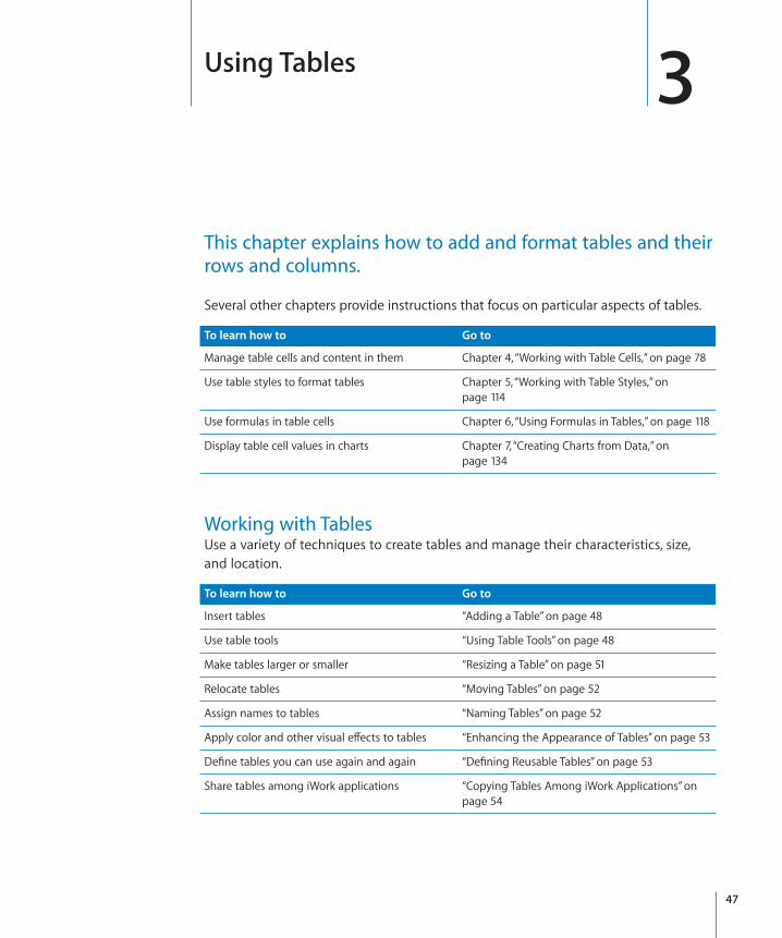
This chapter explains how to add and format tables and their rows and columns.
Several other chapters provide instructions that focus on particular aspects of tables.
To learn how to Go to
Manage table cells and content in them Chapter 4, “Working with Table Cells,” on page 78
Use table styles to format tables Chapter 5, “Working with Table Styles,” on page 114
Use formulas in table cells Chapter 6, “Using Formulas in Tables,” on page 118
Display table cell values in charts Chapter 7, “Creating Charts from Data,” on page 134
Working with TablesUse a variety of techniques to create tables and manage their characteristics, size, and location.
To learn how to Go to
Insert tables “Adding a Table” on page 48
Use table tools “Using Table Tools” on page 48
Make tables larger or smaller “Resizing a Table” on page 51
Relocate tables “Moving Tables” on page 52
Assign names to tables “Naming Tables” on page 52
Apply color and other visual effects to tables “Enhancing the Appearance of Tables” on page 53
Define tables you can use again and again “Defining Reusable Tables” on page 53
Share tables among iWork applications “Copying Tables Among iWork Applications” on page 54
3Using Tables
Adding a TableWhile most templates contain one or more predefined tables, you can add tables to your Numbers spreadsheet.
Here are ways to add a table:�Click Tables in the toolbar and choose a predefined table from the pop-up menu. m
You can add your own predefined tables to the pop-up menu. See “Defining Reusable Tables” on page 53 for instructions.
Choose Insert > Table > m type of table.
To create a new table based on one cell or several adjacent cells in an existing table, m
select the cell or cells and then drag the selection to an empty location on the sheet. To retain values in the selected cells in the original table, hold down the Option key while dragging.
See “Selecting Tables and Their Components” on page 55 to learn about cell selection techniques.
To create a new table based on an entire row or column in an existing table, click the m
reference tab associated with the row or column, press the reference tab, drag the row or column to an empty location on the sheet, and then release the tab. To retain values in the column or row in the original table, hold down the Option key while dragging.
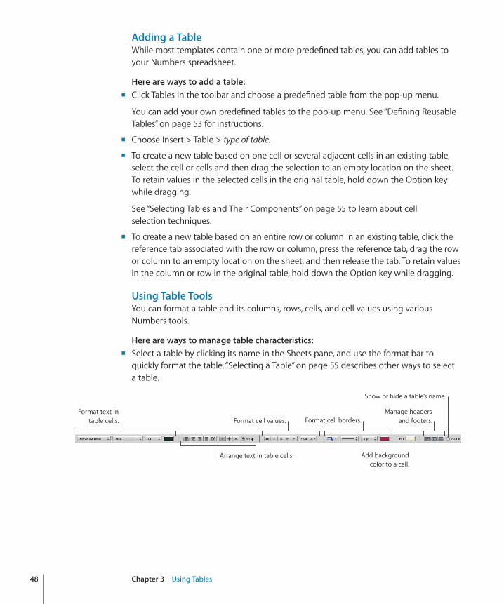
Using Table ToolsYou can format a table and its columns, rows, cells, and cell values using various Numbers tools.
Here are ways to manage table characteristics:�Select a table by clicking its name in the Sheets pane, and use the format bar to m
quickly format the table. “Selecting a Table” on page 55 describes other ways to select a table.
Arrange text in table cells.
Format cell borders.
Add background color to a cell.
Format cell values.Manage headers
and footers.
Show or hide a table’s name.
Format text in table cells.
48 Chapter 3 Using Tables
Chapter 3 Using Tables 49
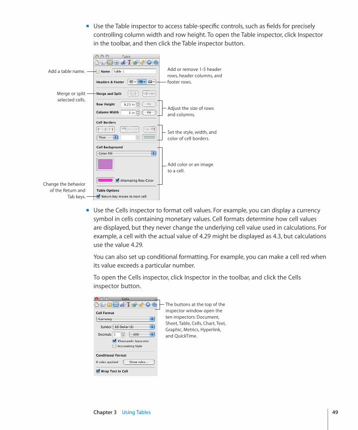
Use the Table inspector to access table-specific controls, such as fields for precisely m
controlling column width and row height. To open the Table inspector, click Inspector in the toolbar, and then click the Table inspector button.
Add a table name.
Merge or split selected cells.
Adjust the size of rows and columns.
Set the style, width, and color of cell borders.
Add color or an image to a cell.
Change the behavior of the Return and
Tab keys.
Add or remove 1-5 header rows, header columns, and footer rows.
Use the Cells inspector to format cell values. For example, you can display a currency m
symbol in cells containing monetary values. Cell formats determine how cell values are displayed, but they never change the underlying cell value used in calculations. For example, a cell with the actual value of 4.29 might be displayed as 4.3, but calculations use the value 4.29.
You can also set up conditional formatting. For example, you can make a cell red when its value exceeds a particular number.
To open the Cells inspector, click Inspector in the toolbar, and click the Cells inspector button.
The buttons at the top of the inspector window open the ten inspectors: Document, Sheet, Table, Cells, Chart, Text, Graphic, Metrics, Hyperlink, and QuickTime.
Use the Graphic inspector to create special visual effects, such as shadows. To m
open the Graphic inspector, click Inspector in the toolbar and then click the Graphic inspector button.
Use table styles to adjust the appearance of tables quickly and consistently. See “ m Using Table Styles” on page 114 for more information.
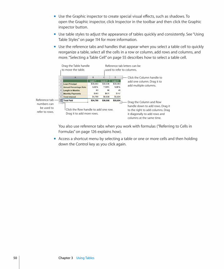
Use the reference tabs and handles that appear when you select a table cell to quickly m
reorganize a table, select all the cells in a row or column, add rows and columns, and more. “Selecting a Table Cell” on page 55 describes how to select a table cell.
Drag the Table handle to move the table.
Reference tab letters can be used to refer to columns.
Click the Column handle to add one column. Drag it to add multiple columns.
Reference tab numbers can
be used to refer to rows.
Drag the Column and Row handle down to add rows. Drag it to the right to add columns. Drag it diagonally to add rows and columns at the same time.
Click the Row handle to add one row. Drag it to add more rows.
You also use reference tabs when you work with formulas (“Referring to Cells in Formulas” on page 126 explains how).
Access a shortcut menu by selecting a table or one or more cells and then holding m
down the Control key as you click again.
50 Chapter 3 Using Tables
Chapter 3 Using Tables 51
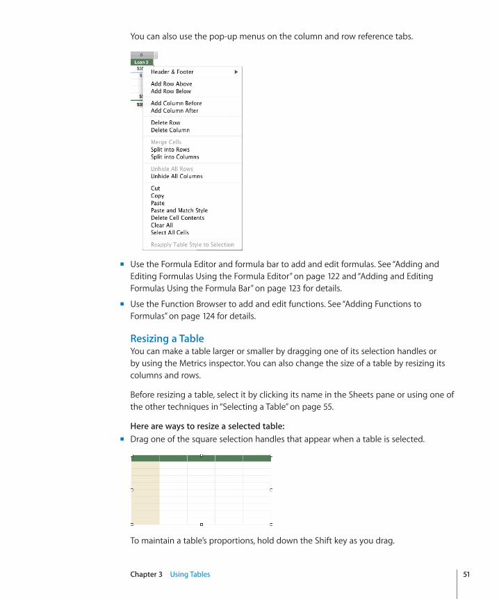
You can also use the pop-up menus on the column and row reference tabs.
Use the Formula Editor and formula bar to add and edit formulas. See “ m Adding and Editing Formulas Using the Formula Editor” on page 122 and “Adding and Editing Formulas Using the Formula Bar” on page 123 for details.
Use the Function Browser to add and edit functions. See “ m Adding Functions to Formulas” on page 124 for details.
Resizing a TableYou can make a table larger or smaller by dragging one of its selection handles or by using the Metrics inspector. You can also change the size of a table by resizing its columns and rows.
Before resizing a table, select it by clicking its name in the Sheets pane or using one of the other techniques in “Selecting a Table” on page 55.
Here are ways to resize a selected table:�Drag one of the square selection handles that appear when a table is selected. m
To maintain a table’s proportions, hold down the Shift key as you drag.
To resize from the table’s center, hold down the Option key as you drag.
To resize a table in one direction, drag a side handle instead of a corner handle.
To resize by specifying exact dimensions, select a table or table cell, click Inspector in m
the toolbar, and then click the Metrics inspector button. Using the Metrics inspector, you can specify a new width and height, and you can change the table’s distance from the margins by using the Position fields.
To resize by adjusting the dimensions of rows and columns, see “ m Resizing Table Rows and Columns” on page 65.
Moving TablesYou can move a table by dragging it, or you can relocate a table using the Metrics inspector.
Here are ways to move a table:�If the table isn’t selected or if the entire table is selected, press the edge of the table m
and drag it.
If a table cell is selected, drag the table using the Table handle in the upper left.
To constrain the movement to horizontal, vertical, or 45 degrees, hold down the Shift m
key as you drag.
To move a table more precisely, click any cell, click Inspector in the toolbar, click the m
Metrics inspector button, and then use the Position fields to relocate the table.
To copy a table and then move the copy, hold down the Option key, press at the edge m
of an unselected table or an entire table that’s selected, and drag.
Naming TablesEvery Numbers table has a name that’s displayed in the Sheets pane and can optionally be displayed above the table. The default table name (Table 1, Table 2, and so forth) can be changed, hidden, and formatted.
Here are ways to work with table names:�To change the name, double-click it in the Sheets pane and type the new name. m
You can also click in the table and change its name using the Table inspector’s Name field.
On any sheet, two tables can’t have the same name.
To show a table’s name on the sheet canvas, click in the table and then select Name in m
the format bar or the Table inspector.
To hide the table name on the sheet, deselect Name.
To format a name displayed on the sheet canvas, select the table, click the table name m
on the sheet canvas to activate the name for formatting, and use the format bar, Fonts window, or Text pane of the Text inspector.
52 Chapter 3 Using Tables
Chapter 3 Using Tables 53
To increase the distance between the table name and the table body, select Name in m
the Table inspector, click the name on the canvas, and then use the Text inspector to modify the After Paragraph spacing.
Enhancing the Appearance of TablesYou can apply color, use images, and use other formatting techniques to enhance the visual appeal of your tables.
Here are ways to enhance a table’s appearance:�You can fill the background of an entire table or individual cells with different kinds of m
color effects or with an image. See “Filling Objects with Colors or Images” on page 225 for instructions.
You can change the thickness and color of borders around a table and its cells, as m
“Formatting Table Cell Borders” on page 87 describes.
You can adjust the attributes of text in table cells, including header and footer cells. m
See “Formatting Text Size and Appearance” on page 165 and “Setting Text Alignment, Spacing, and Color” on page 172 for details.
When you’ve created a visual effect that you want to reuse, you can copy and paste it; select the table or cells whose effects you want to reuse, choose Format > Copy Style, select the table or cells you want to format, and then choose Format > Paste Style. You can also use table styles to replicate formatting you’ve applied to a table, as “Using Table Styles” on page 114 describes.
Defining Reusable TablesYou can add your own tables to the menu of predefined tables that appears when you click Tables in the toolbar or choose Insert > Table. Reusable tables have the table style and structure of your choice and can contain content (header text, formulas, and so on).
To define a reusable table: 1 Select a table.
2 Define a table style for the table.
The table style determines the formatting of borders, background, and text in the table’s cells.
One way to define the table style is by following the instructions in “Modifying Table Style Attributes” on page 115 and “Copying and Pasting Table Styles” on page 116.
Alternatively, you can apply your customized table structure and content to the reusable table, but give it the table’s original default style instead of your own. Step 7 describes how to use this option.
3 Define the table’s structure.
To resize the table, see “Resizing a Table” on page 51 and “Resizing Table Rows and Columns” on page 65.
To define columns and rows, see “Working with Rows and Columns in Tables” on page 59.
To split or merge table cells, see “Splitting Table Cells” on page 87 or “Merging Table Cells” on page 86.
4 Add and format any content you want to reuse. See “Putting Content into Table Cells” on page 78 for instructions. Any formulas you add should refer only to cells in the table you’re defining.
5 Choose Format > Advanced > Capture Table.
6 Type a name for the table.
7 Select “Use the default style from the document” if you want the table to be styled using the default table style in effect when the table is added to the spreadsheet. Otherwise the table style used is the one you defined in step 2.
8 Click OK.
A copy of your reusable table can now be added to the current spreadsheet by choosing it from the menu of predefined tables that appears when you click Tables in the toolbar or choose Insert > Table.
To rearrange, rename, or delete tables on the menu, choose Format > Advanced > Manage Tables. Double-click a name to change the name of a predefined table. Select a table and click the up or down arrow button to move it up or down in the list of tables. Click the Delete (–) button to remove a table. Click Done when you’ve finished.
The table and menu changes apply only to the current spreadsheet. If you want your reusable tables and menu changes to be available in other spreadsheets, save the spreadsheet as a template, using the instructions in “Saving a Custom Template” on page 249.
Copying Tables Among iWork ApplicationsYou can copy a table from one iWork application to another.
The table retains its appearance, data, and other attributes, but some Numbers features aren’t supported in the other applications:
Rows or columns that are hidden in Numbers are removed. Â
Comments added to Numbers table cells aren’t copied. Â
To copy a table from one iWork application to another:� 1 Select the table you want to copy, as “Selecting a Table” on page 55 describes.
54 Chapter 3 Using Tables
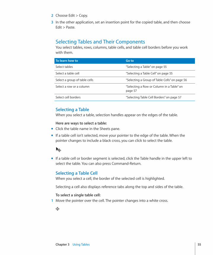
Chapter 3 Using Tables 55
2 Choose Edit > Copy.
3 In the other application, set an insertion point for the copied table, and then choose Edit > Paste.
Selecting Tables and Their ComponentsYou select tables, rows, columns, table cells, and table cell borders before you work with them.
To learn how to Go to
Select tables “Selecting a Table” on page 55
Select a table cell “Selecting a Table Cell” on page 55
Select a group of table cells “Selecting a Group of Table Cells” on page 56
Select a row or a column “Selecting a Row or Column in a Table” on page 57
Select cell borders “Selecting Table Cell Borders” on page 57
Selecting a TableWhen you select a table, selection handles appear on the edges of the table.
Here are ways to select a table:�Click the table name in the Sheets pane. m
If a table cell isn’t selected, move your pointer to the edge of the table. When the m
pointer changes to include a black cross, you can click to select the table.
If a table cell or border segment is selected, click the Table handle in the upper left to m
select the table. You can also press Command-Return.
Selecting a Table CellWhen you select a cell, the border of the selected cell is highlighted.
Selecting a cell also displays reference tabs along the top and sides of the table.
To select a single table cell:� 1 Move the pointer over the cell. The pointer changes into a white cross.
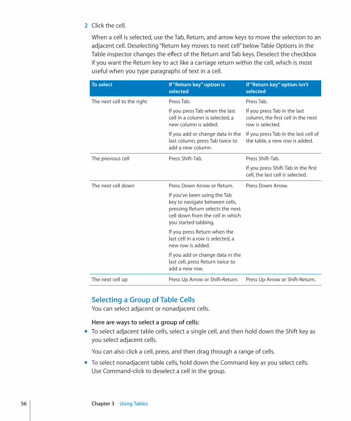
2 Click the cell.
When a cell is selected, use the Tab, Return, and arrow keys to move the selection to an adjacent cell. Deselecting “Return key moves to next cell” below Table Options in the Table inspector changes the effect of the Return and Tab keys. Deselect the checkbox if you want the Return key to act like a carriage return within the cell, which is most useful when you type paragraphs of text in a cell.
To select If “Return key” option is selected
If “Return key” option isn’t selected
The next cell to the right Press Tab.
If you press Tab when the last cell in a column is selected, a new column is added.
If you add or change data in the last column, press Tab twice to add a new column.
Press Tab.
If you press Tab in the last column, the first cell in the next row is selected.
If you press Tab in the last cell of the table, a new row is added.
The previous cell Press Shift-Tab. Press Shift-Tab.
If you press Shift-Tab in the first cell, the last cell is selected.
The next cell down Press Down Arrow or Return.
If you’ve been using the Tab key to navigate between cells, pressing Return selects the next cell down from the cell in which you started tabbing.
If you press Return when the last cell in a row is selected, a new row is added.
If you add or change data in the last cell, press Return twice to add a new row.
Press Down Arrow.
The next cell up Press Up Arrow or Shift-Return. Press Up Arrow or Shift-Return.
Selecting a Group of Table CellsYou can select adjacent or nonadjacent cells.
Here are ways to select a group of cells:�To select adjacent table cells, select a single cell, and then hold down the Shift key as m
you select adjacent cells.
You can also click a cell, press, and then drag through a range of cells.
To select nonadjacent table cells, hold down the Command key as you select cells. m
Use Command-click to deselect a cell in the group.
56 Chapter 3 Using Tables
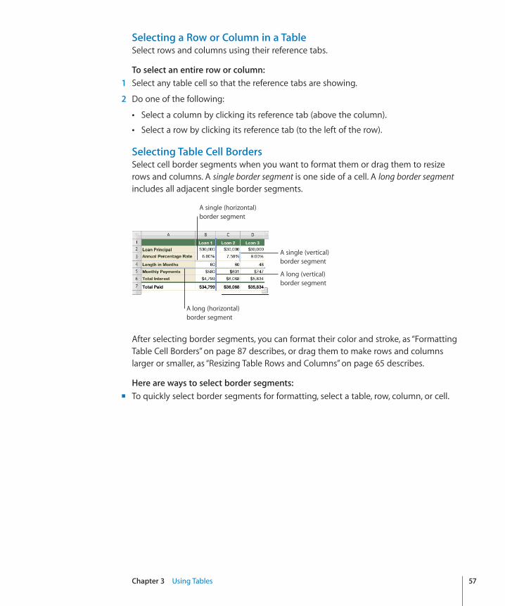
Chapter 3 Using Tables 57
Selecting a Row or Column in a TableSelect rows and columns using their reference tabs.
To select an entire row or column:� 1 Select any table cell so that the reference tabs are showing.
2 Do one of the following:
Select a column by clicking its reference tab (above the column). Â
Select a row by clicking its reference tab (to the left of the row). Â
Selecting Table Cell BordersSelect cell border segments when you want to format them or drag them to resize rows and columns. A single border segment is one side of a cell. A long border segment includes all adjacent single border segments.
A single (horizontal) border segment
A long (vertical) border segment
A long (horizontal) border segment
A single (vertical) border segment
After selecting border segments, you can format their color and stroke, as “Formatting Table Cell Borders” on page 87 describes, or drag them to make rows and columns larger or smaller, as “Resizing Table Rows and Columns” on page 65 describes.
Here are ways to select border segments:�To quickly select border segments for formatting, select a table, row, column, or cell. m
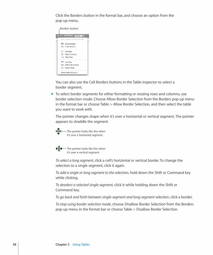
Click the Borders button in the format bar, and choose an option from the pop-up menu.
Borders button
You can also use the Cell Borders buttons in the Table inspector to select a border segment.
To select border segments for either formatting or resizing rows and columns, use m
border selection mode. Choose Allow Border Selection from the Borders pop-up menu in the format bar or choose Table > Allow Border Selection, and then select the table you want to work with.
The pointer changes shape when it’s over a horizontal or vertical segment. The pointer appears to straddle the segment.
The pointer looks like this when it’s over a horizontal segment.
The pointer looks like this when it’s over a vertical segment.
To select a long segment, click a cell’s horizontal or vertical border. To change the selection to a single segment, click it again.
To add a single or long segment to the selection, hold down the Shift or Command key while clicking.
To deselect a selected single segment, click it while holding down the Shift or Command key.
To go back and forth between single-segment and long-segment selection, click a border.
To stop using border selection mode, choose Disallow Border Selection from the Borders pop-up menu in the format bar or choose Table > Disallow Border Selection.
58 Chapter 3 Using Tables
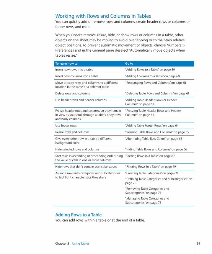
Chapter 3 Using Tables 59
Working with Rows and Columns in TablesYou can quickly add or remove rows and columns, create header rows or columns or footer rows, and more.
When you insert, remove, resize, hide, or show rows or columns in a table, other objects on the sheet may be moved to avoid overlapping or to maintain relative object positions. To prevent automatic movement of objects, choose Numbers > Preferences and in the General pane deselect “Automatically move objects when tables resize.”
To learn how to Go to
Insert new rows into a table “Adding Rows to a Table” on page 59
Insert new columns into a table “Adding Columns to a Table” on page 60
Move or copy rows and columns to a different location in the same or a different table
“Rearranging Rows and Columns” on page 61
Delete rows and columns “Deleting Table Rows and Columns” on page 61
Use header rows and header columns “Adding Table Header Rows or Header Columns” on page 62
Freeze header rows and columns so they remain in view as you scroll through a table’s body rows and body columns
“Freezing Table Header Rows and Header Columns” on page 64
Use footer rows “Adding Table Footer Rows” on page 64
Resize rows and columns “Resizing Table Rows and Columns” on page 65
Give every other row in a table a different background color
“Alternating Table Row Colors” on page 66
Hide selected rows and columns “Hiding Table Rows and Columns” on page 66
Sort rows in ascending or descending order using the value of cells in one or more columns
“Sorting Rows in a Table” on page 67
Hide rows that don’t contain particular values “Filtering Rows in a Table” on page 69
Arrange rows into categories and subcategories to highlight characteristics they share
“Creating Table Categories” on page 69
“Defining Table Categories and Subcategories” on page 70
“Removing Table Categories and Subcategories” on page 75
“Managing Table Categories and Subcategories” on page 75
Adding Rows to a TableYou can add rows within a table or at the end of a table.
If the table contains a footer row, rows added at the bottom of the table are added above the footer row. If the table has filtering criteria associated with it, you can’t add new rows until you stop filtering rows; see “Filtering Rows in a Table” on page 69 for instructions.
If all the body cells in a column above the new row contain the same formula or cell control, the formula or cell control is repeated in the new row.
Here are ways to add rows:�To add a row above a selected cell, press Option-Up Arrow. m
To add a row below a selected cell, press Option-Down Arrow.
You can add a single row above or below a particular row by holding the pointer over m
a row’s reference tab to see its menu arrow, clicking the arrow, and then choosing Add Row Above or Add Row Below from the pop-up menu.
You can also click in a row and then choose Table > Add Row Above or Table > Add Row Below.
To add multiple rows, select the number of rows you want to add (select three rows if m
you want to add three rows). To add rows after a particular row, make sure the bottom row selected is the one after which you want the new rows added; to add rows before a particular row, make sure the top row selected is the one before which you want the new rows added. Then choose Table > Add Rows Above or Table > Add Rows Below.
To add a row at the end of the table, press Return while the last cell is selected. m
Press Return twice if you’ve just added or changed the cell value and you’re still editing the cell.
If “Return key moves to next cell” below Table Options in the Table inspector isn’t selected, press Tab instead from the last cell in the row.
To add one or more rows at the end of the table, you can use the Row handle in the m
lower left, visible when a cell is selected.
To add a row at the end of the table, click the Row handle once.
To add multiple rows at the end of the table, drag the Row handle or the Column and Row handle (in the lower right) down.
To add rows and columns at the same time, drag the Column and Row handle diagonally.
You can split cells into two equal rows. “ m Splitting Table Cells” on page 87 describes how.
Adding Columns to a TableHere are ways to add columns:�To add a column after a selected cell, press Option-Right Arrow. m
To add a column before a selected cell, press Option-Left Arrow.
60 Chapter 3 Using Tables
Chapter 3 Using Tables 61
To add a single column, hold the pointer over a column’s reference tab to see its menu m
arrow. Click the arrow and then choose Add Column Before or Add Column After from the pop-up menu. You can also select a column and then choose these commands from the Table menu.
To add multiple columns, select the number of columns you want to add (select three m
columns to add three columns). To add columns after a particular column, make sure the rightmost column selected is the one after which you want the new columns added; to add columns before a particular column, make sure the leftmost column selected is the one before which you want the new columns added. Then choose one of the commands above.
You can use the Tab key to add a column to the right side of the table when “Return m
key moves to next cell” below Table Options in the Table inspector is selected.
Press Tab once when the last cell is selected. Press Tab twice if you’ve just added or changed the cell value and you’re still editing the cell.
To add one or more columns to the right side of a table, you can use the Column m
handle in the upper right, visible when a cell is selected.
To add a column to the right side of the table, click the Column handle once.
To add multiple columns to the right side of the table, drag the Column handle or the Column and Row handle (in the lower right) to the right.
To add rows and columns at the same time, drag the Column and Row handle diagonally.
You can split cells into two equal columns. “ m Splitting Table Cells” on page 87 explains how.
Rearranging Rows and ColumnsUsing a row’s or column’s reference tab, you can move or copy the row or column to a different location in the same table or another table.
Here are ways to rearrange rows and columns:�To move a column or row to a different location in the same table or a different table, m
click the column or row reference tab, press, and then drag the reference tab. Release the tab when the bold line highlights where you want to insert the column or row.
To insert a copy of a row or column elsewhere in the table or in another table, click m
the reference tab, and then press and hold down the Option key and the reference tab while you drag the column or row to the desired location.
You can also copy or move a single cell or a group of adjacent cells within or between tables. See “Copying and Moving Cells” on page 88 for instructions.
Deleting Table Rows and ColumnsThere are several techniques available for deleting one or more rows or columns of a table.
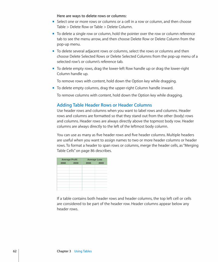
Here are ways to delete rows or columns:�Select one or more rows or columns or a cell in a row or column, and then choose m
Table > Delete Row or Table > Delete Column.
To delete a single row or column, hold the pointer over the row or column reference m
tab to see the menu arrow, and then choose Delete Row or Delete Column from the pop-up menu.
To delete several adjacent rows or columns, select the rows or columns and then m
choose Delete Selected Rows or Delete Selected Columns from the pop-up menu of a selected row’s or column’s reference tab.
To delete empty rows, drag the lower-left Row handle up or drag the lower-right m
Column handle up.
To remove rows with content, hold down the Option key while dragging.
To delete empty columns, drag the upper-right Column handle inward. m
To remove columns with content, hold down the Option key while dragging.
Adding Table Header Rows or Header ColumnsUse header rows and columns when you want to label rows and columns. Header rows and columns are formatted so that they stand out from the other (body) rows and columns. Header rows are always directly above the topmost body row. Header columns are always directly to the left of the leftmost body column.
You can use as many as five header rows and five header columns. Multiple headers are useful when you want to assign names to two or more header columns or header rows. To format a header to span rows or columns, merge the header cells, as “Merging Table Cells” on page 86 describes.
If a table contains both header rows and header columns, the top left cell or cells are considered to be part of the header row. Header columns appear below any header rows.
62 Chapter 3 Using Tables
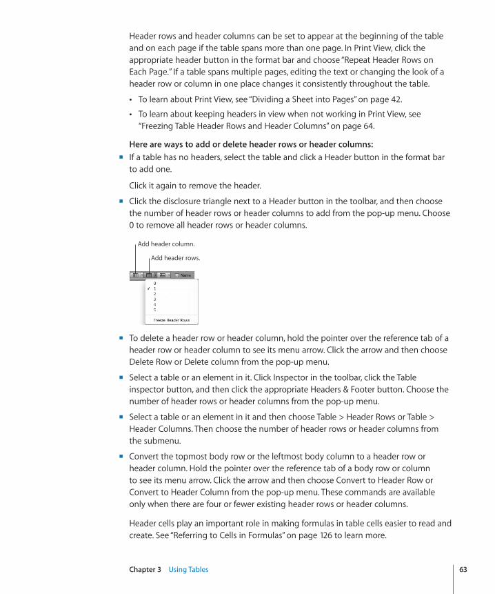
Chapter 3 Using Tables 63
Header rows and header columns can be set to appear at the beginning of the table and on each page if the table spans more than one page. In Print View, click the appropriate header button in the format bar and choose “Repeat Header Rows on Each Page.” If a table spans multiple pages, editing the text or changing the look of a header row or column in one place changes it consistently throughout the table.
To learn about Print View, see “ Â Dividing a Sheet into Pages” on page 42.
To learn about keeping headers in view when not working in Print View, see “Freezing Table Header Rows and Header Columns” on page 64.
Here are ways to add or delete header rows or header columns:�If a table has no headers, select the table and click a Header button in the format bar m
to add one.
Click it again to remove the header.
Click the disclosure triangle next to a Header button in the toolbar, and then choose m
the number of header rows or header columns to add from the pop-up menu. Choose 0 to remove all header rows or header columns.
Add header column.
Add header rows.
To delete a header row or header column, hold the pointer over the reference tab of a m
header row or header column to see its menu arrow. Click the arrow and then choose Delete Row or Delete column from the pop-up menu.
Select a table or an element in it. Click Inspector in the toolbar, click the Table m
inspector button, and then click the appropriate Headers & Footer button. Choose the number of header rows or header columns from the pop-up menu.
Select a table or an element in it and then choose Table > Header Rows or Table > m
Header Columns. Then choose the number of header rows or header columns from the submenu.
Convert the topmost body row or the leftmost body column to a header row or m
header column. Hold the pointer over the reference tab of a body row or column to see its menu arrow. Click the arrow and then choose Convert to Header Row or Convert to Header Column from the pop-up menu. These commands are available only when there are four or fewer existing header rows or header columns.
Header cells play an important role in making formulas in table cells easier to read and create. See “Referring to Cells in Formulas” on page 126 to learn more.
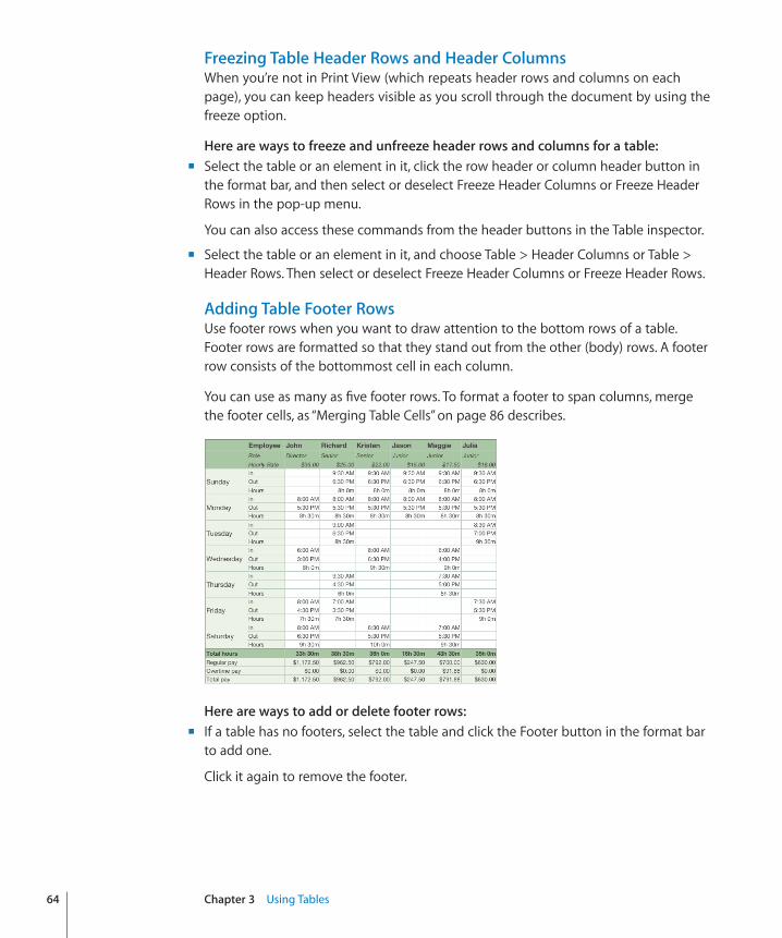
Freezing Table Header Rows and Header ColumnsWhen you’re not in Print View (which repeats header rows and columns on each page), you can keep headers visible as you scroll through the document by using the freeze option.
Here are ways to freeze and unfreeze header rows and columns for a table:� Select the table or an element in it, click the row header or column header button in m
the format bar, and then select or deselect Freeze Header Columns or Freeze Header Rows in the pop-up menu.
You can also access these commands from the header buttons in the Table inspector.
Select the table or an element in it, and choose Table > Header Columns or Table > m
Header Rows. Then select or deselect Freeze Header Columns or Freeze Header Rows.
Adding Table Footer RowsUse footer rows when you want to draw attention to the bottom rows of a table. Footer rows are formatted so that they stand out from the other (body) rows. A footer row consists of the bottommost cell in each column.
You can use as many as five footer rows. To format a footer to span columns, merge the footer cells, as “Merging Table Cells” on page 86 describes.
Here are ways to add or delete footer rows:�If a table has no footers, select the table and click the Footer button in the format bar m
to add one.
Click it again to remove the footer.
64 Chapter 3 Using Tables
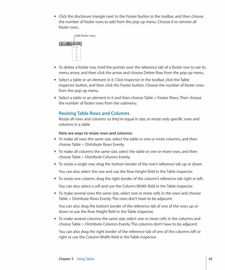
Chapter 3 Using Tables 65
Click the disclosure triangle next to the Footer button in the toolbar, and then choose m
the number of footer rows to add from the pop-up menu. Choose 0 to remove all footer rows.
Add footer rows.
To delete a footer row, hold the pointer over the reference tab of a footer row to see its m
menu arrow, and then click the arrow and choose Delete Row from the pop-up menu.
Select a table or an element in it. Click Inspector in the toolbar, click the Table m
inspector button, and then click the Footer button. Choose the number of footer rows from the pop-up menu.
Select a table or an element in it and then choose Table > Footer Rows. Then choose m
the number of footer rows from the submenu.
Resizing Table Rows and ColumnsResize all rows and columns so they’re equal in size, or resize only specific rows and columns in a table.
Here are ways to resize rows and columns:�To make all rows the same size, select the table or one or more columns, and then m
choose Table > Distribute Rows Evenly.
To make all columns the same size, select the table or one or more rows, and then m
choose Table > Distribute Columns Evenly.
To resize a single row, drag the bottom border of the row’s reference tab up or down. m
You can also select the row and use the Row Height field in the Table inspector.
To resize one column, drag the right border of the column’s reference tab right or left. m
You can also select a cell and use the Column Width field in the Table inspector.
To make several rows the same size, select one or more cells in the rows and choose m
Table > Distribute Rows Evenly. The rows don’t have to be adjacent.
You can also drag the bottom border of the reference tab of one of the rows up or down or use the Row Height field in the Table inspector.
To make several columns the same size, select one or more cells in the columns and m
choose Table > Distribute Columns Evenly. The columns don’t have to be adjacent.
You can also drag the right border of the reference tab of one of the columns left or right or use the Column Width field in the Table inspector.
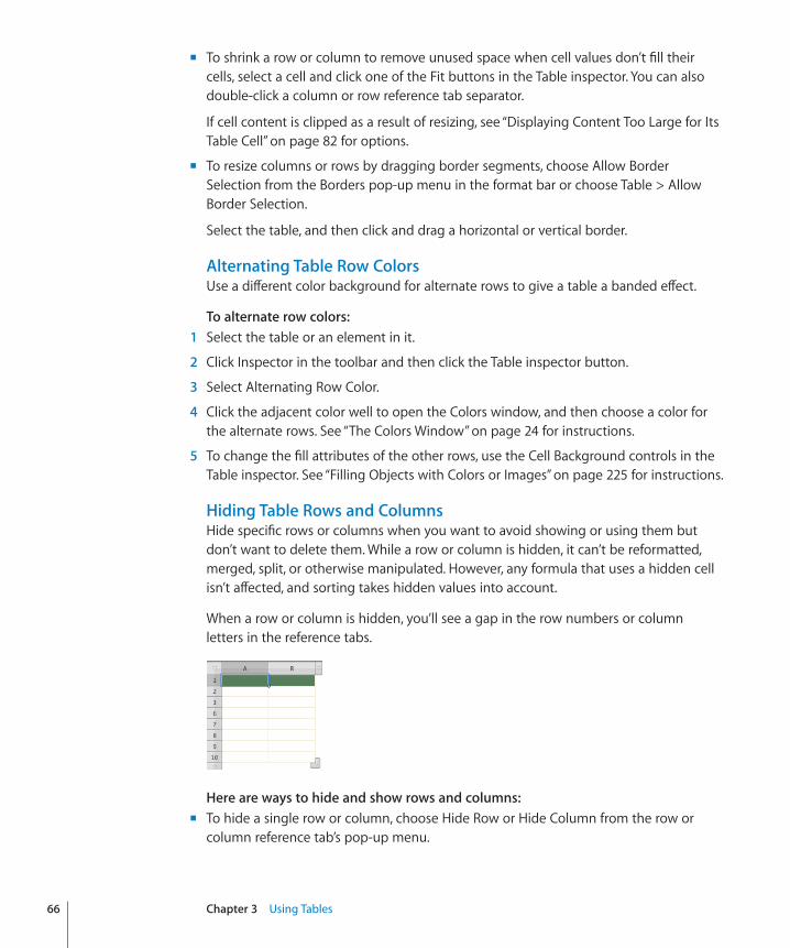
To shrink a row or column to remove unused space when cell values don’t fill their m
cells, select a cell and click one of the Fit buttons in the Table inspector. You can also double-click a column or row reference tab separator.
If cell content is clipped as a result of resizing, see “Displaying Content Too Large for Its Table Cell” on page 82 for options.
To resize columns or rows by dragging border segments, choose Allow Border m
Selection from the Borders pop-up menu in the format bar or choose Table > Allow Border Selection.
Select the table, and then click and drag a horizontal or vertical border.
Alternating Table Row ColorsUse a different color background for alternate rows to give a table a banded effect.
To alternate row colors:� 1 Select the table or an element in it.
2 Click Inspector in the toolbar and then click the Table inspector button.
3 Select Alternating Row Color.
4 Click the adjacent color well to open the Colors window, and then choose a color for the alternate rows. See “The Colors Window” on page 24 for instructions.
5 To change the fill attributes of the other rows, use the Cell Background controls in the Table inspector. See “Filling Objects with Colors or Images” on page 225 for instructions.
Hiding Table Rows and ColumnsHide specific rows or columns when you want to avoid showing or using them but don’t want to delete them. While a row or column is hidden, it can’t be reformatted, merged, split, or otherwise manipulated. However, any formula that uses a hidden cell isn’t affected, and sorting takes hidden values into account.
When a row or column is hidden, you’ll see a gap in the row numbers or column letters in the reference tabs.
Here are ways to hide and show rows and columns:�To hide a single row or column, choose Hide Row or Hide Column from the row or m
column reference tab’s pop-up menu.
66 Chapter 3 Using Tables
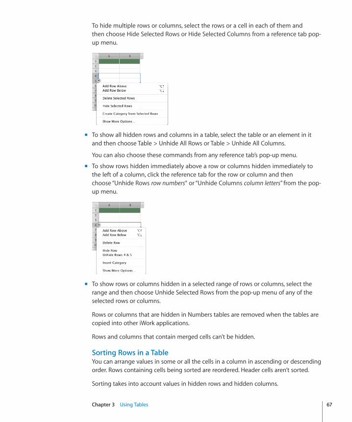
Chapter 3 Using Tables 67
To hide multiple rows or columns, select the rows or a cell in each of them and then choose Hide Selected Rows or Hide Selected Columns from a reference tab pop-up menu.
To show all hidden rows and columns in a table, select the table or an element in it m
and then choose Table > Unhide All Rows or Table > Unhide All Columns.
You can also choose these commands from any reference tab’s pop-up menu.
To show rows hidden immediately above a row or columns hidden immediately to m
the left of a column, click the reference tab for the row or column and then choose “Unhide Rows row numbers“ or “Unhide Columns column letters” from the pop-up menu.
To show rows or columns hidden in a selected range of rows or columns, select the m
range and then choose Unhide Selected Rows from the pop-up menu of any of the selected rows or columns.
Rows or columns that are hidden in Numbers tables are removed when the tables are copied into other iWork applications.
Rows and columns that contain merged cells can’t be hidden.
Sorting Rows in a TableYou can arrange values in some or all the cells in a column in ascending or descending order. Rows containing cells being sorted are reordered. Header cells aren’t sorted.
Sorting takes into account values in hidden rows and hidden columns.
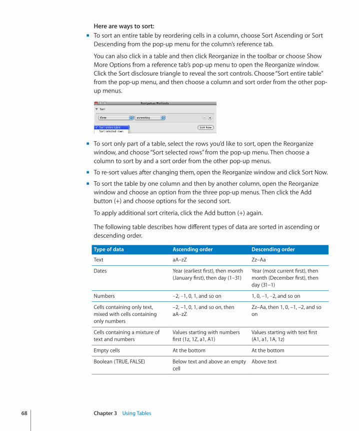
Here are ways to sort:�To sort an entire table by reordering cells in a column, choose Sort Ascending or Sort m
Descending from the pop-up menu for the column’s reference tab.
You can also click in a table and then click Reorganize in the toolbar or choose Show More Options from a reference tab’s pop-up menu to open the Reorganize window. Click the Sort disclosure triangle to reveal the sort controls. Choose “Sort entire table” from the pop-up menu, and then choose a column and sort order from the other pop-up menus.
To sort only part of a table, select the rows you’d like to sort, open the Reorganize m
window, and choose “Sort selected rows” from the pop-up menu. Then choose a column to sort by and a sort order from the other pop-up menus.
To re-sort values after changing them, open the Reorganize window and click Sort Now. m
To sort the table by one column and then by another column, open the Reorganize m
window and choose an option from the three pop-up menus. Then click the Add button (+) and choose options for the second sort.
To apply additional sort criteria, click the Add button (+) again.
The following table describes how different types of data are sorted in ascending or descending order.
Type of data Ascending order Descending order
Text aA–zZ Zz–Aa
Dates Year (earliest first), then month (January first), then day (1–31)
Year (most current first), then month (December first), then day (31–1)
Numbers –2, –1, 0, 1, and so on 1, 0, –1, –2, and so on
Cells containing only text, mixed with cells containing only numbers
–2, –1, 0, 1, and so on, then aA–zZ
Zz–Aa, then 1, 0, –1, –2, and so on
Cells containing a mixture of text and numbers
Values starting with numbers first (1z, 1Z, a1, A1)
Values starting with text first (A1, a1, 1A, 1z)
Empty cells At the bottom At the bottom
Boolean (TRUE, FALSE) Below text and above an empty cell
Above text
68 Chapter 3 Using Tables
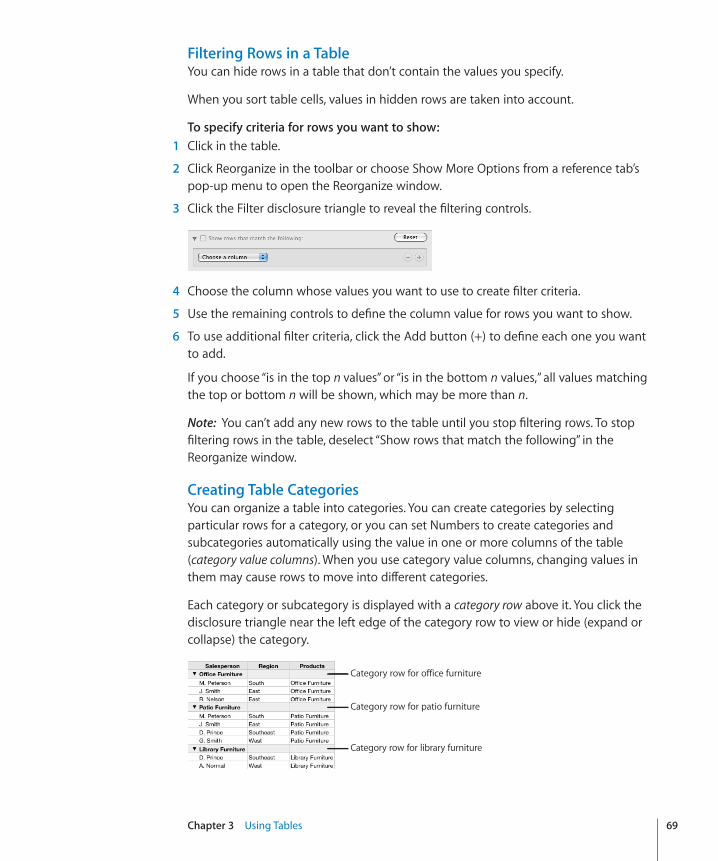
Chapter 3 Using Tables 69
Filtering Rows in a TableYou can hide rows in a table that don’t contain the values you specify.
When you sort table cells, values in hidden rows are taken into account.
To specify criteria for rows you want to show:� 1 Click in the table.
2 Click Reorganize in the toolbar or choose Show More Options from a reference tab’s pop-up menu to open the Reorganize window.
3 Click the Filter disclosure triangle to reveal the filtering controls.
4 Choose the column whose values you want to use to create filter criteria.
5 Use the remaining controls to define the column value for rows you want to show.
6 To use additional filter criteria, click the Add button (+) to define each one you want to add.
If you choose “is in the top n values” or “is in the bottom n values,” all values matching the top or bottom n will be shown, which may be more than n.
Note: You can’t add any new rows to the table until you stop filtering rows. To stop filtering rows in the table, deselect “Show rows that match the following” in the Reorganize window.
Creating Table CategoriesYou can organize a table into categories. You can create categories by selecting particular rows for a category, or you can set Numbers to create categories and subcategories automatically using the value in one or more columns of the table (category value columns). When you use category value columns, changing values in them may cause rows to move into different categories.
Each category or subcategory is displayed with a category row above it. You click the disclosure triangle near the left edge of the category row to view or hide (expand or collapse) the category.
Category row for office furniture
Category row for patio furniture
Category row for library furniture
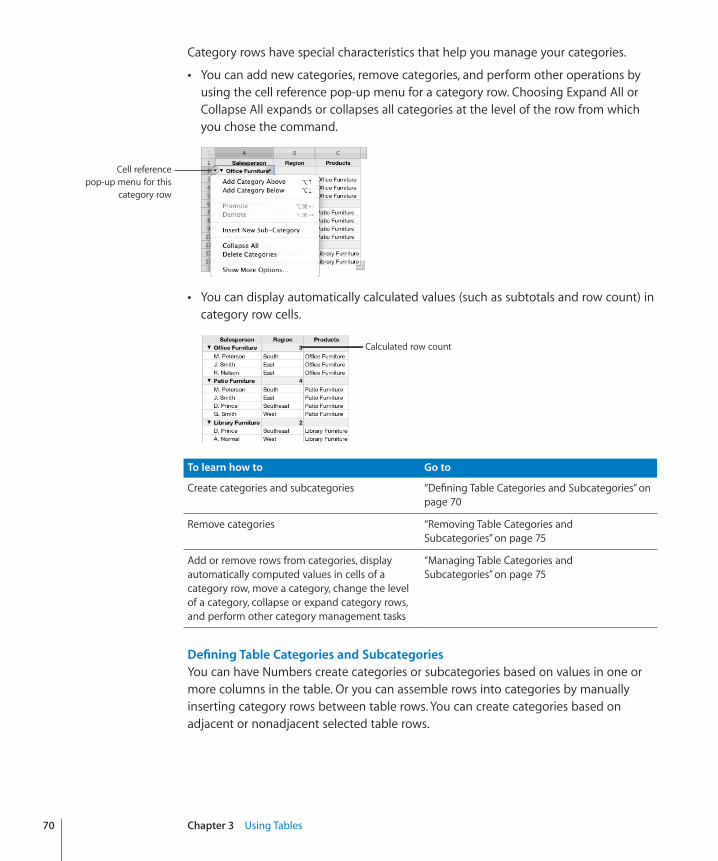
Category rows have special characteristics that help you manage your categories.
You can add new categories, remove categories, and perform other operations by Âusing the cell reference pop-up menu for a category row. Choosing Expand All or Collapse All expands or collapses all categories at the level of the row from which you chose the command.
Cell reference pop-up menu for this
category row
You can display automatically calculated values (such as subtotals and row count) in Âcategory row cells.
Calculated row count
To learn how to Go to
Create categories and subcategories “Defining Table Categories and Subcategories” on page 70
Remove categories “Removing Table Categories and Subcategories” on page 75
Add or remove rows from categories, display automatically computed values in cells of a category row, move a category, change the level of a category, collapse or expand category rows, and perform other category management tasks
“Managing Table Categories and Subcategories” on page 75
Defining Table Categories and SubcategoriesYou can have Numbers create categories or subcategories based on values in one or more columns in the table. Or you can assemble rows into categories by manually inserting category rows between table rows. You can create categories based on adjacent or nonadjacent selected table rows.
70 Chapter 3 Using Tables
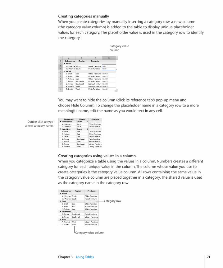
Chapter 3 Using Tables 71
Creating categories manuallyWhen you create categories by manually inserting a category row, a new column (the category value column) is added to the table to display unique placeholder values for each category. The placeholder value is used in the category row to identify the category.
Category value column
You may want to hide the column (click its reference tab’s pop-up menu and choose Hide Column). To change the placeholder name in a category row to a more meaningful name, edit the name as you would text in any cell.
Double-click to typea new category name.
Creating categories using values in a columnWhen you categorize a table using the values in a column, Numbers creates a different category for each unique value in the column. The column whose value you use to create categories is the category value column. All rows containing the same value in the category value column are placed together in a category. The shared value is used as the category name in the category row.
Category row
Category value column
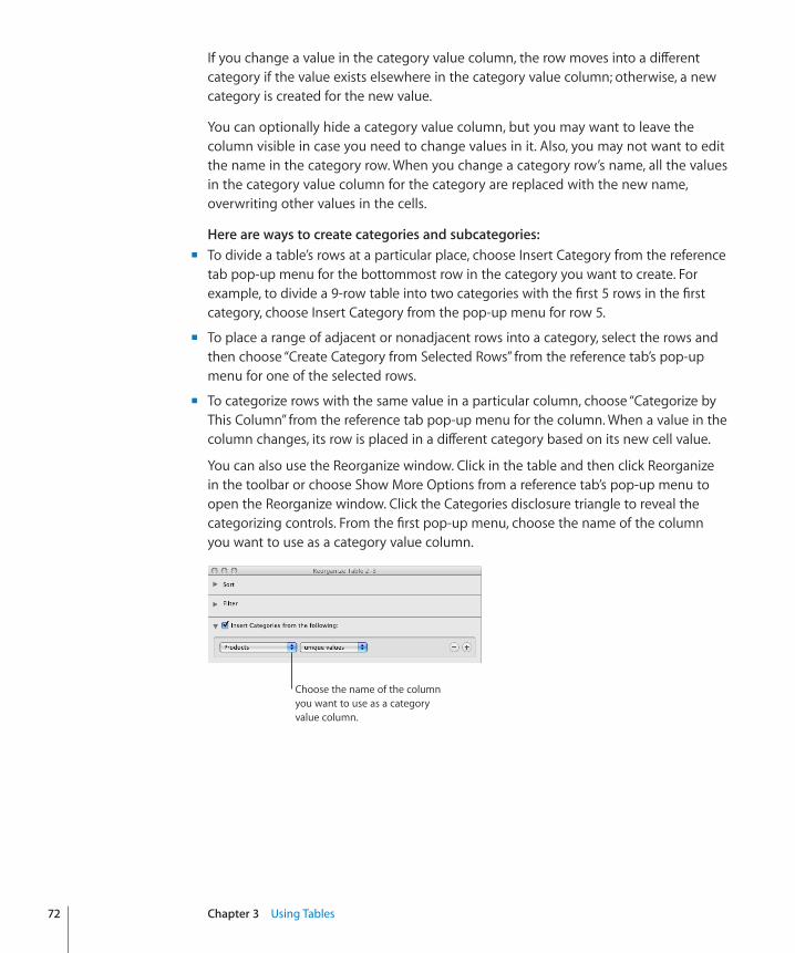
If you change a value in the category value column, the row moves into a different category if the value exists elsewhere in the category value column; otherwise, a new category is created for the new value.
You can optionally hide a category value column, but you may want to leave the column visible in case you need to change values in it. Also, you may not want to edit the name in the category row. When you change a category row’s name, all the values in the category value column for the category are replaced with the new name, overwriting other values in the cells.
Here are ways to create categories and subcategories:�To divide a table’s rows at a particular place, choose Insert Category from the reference m
tab pop-up menu for the bottommost row in the category you want to create. For example, to divide a 9-row table into two categories with the first 5 rows in the first category, choose Insert Category from the pop-up menu for row 5.
To place a range of adjacent or nonadjacent rows into a category, select the rows and m
then choose “Create Category from Selected Rows” from the reference tab’s pop-up menu for one of the selected rows.
To categorize rows with the same value in a particular column, choose “Categorize by m
This Column” from the reference tab pop-up menu for the column. When a value in the column changes, its row is placed in a different category based on its new cell value.
You can also use the Reorganize window. Click in the table and then click Reorganize in the toolbar or choose Show More Options from a reference tab’s pop-up menu to open the Reorganize window. Click the Categories disclosure triangle to reveal the categorizing controls. From the first pop-up menu, choose the name of the column you want to use as a category value column.
Choose the name of the column you want to use as a category value column.
72 Chapter 3 Using Tables
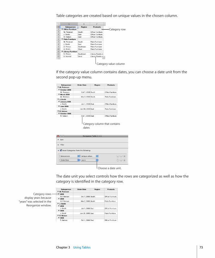
Chapter 3 Using Tables 73
Table categories are created based on unique values in the chosen column.
Category row
Category value column
If the category value column contains dates, you can choose a date unit from the second pop-up menu.
Category column that contains dates
Choose a date unit.
The date unit you select controls how the rows are categorized as well as how the category is identified in the category row.
Category rowsdisplay years because
“years” was selected in the Reorganize window.
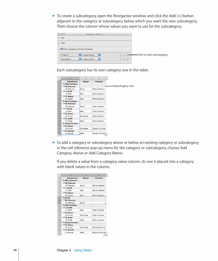
To create a subcategory, open the Reorganize window, and click the Add (+) button m
adjacent to the category or subcategory below which you want the new subcategory. Then choose the column whose values you want to use for the subcategory.
Click to add subcategory.
Each subcategory has its own category row in the table.
Subcategory row
To add a category or subcategory above or below an existing category or subcategory, m
in the cell reference pop-up menu for the category or subcategory, choose Add Category Above or Add Category Below.
If you delete a value from a category value column, its row is placed into a category with blank values in the column.
74 Chapter 3 Using Tables
Chapter 3 Using Tables 75
If you delete all rows from a category, the category is removed from the table.
Removing Table Categories and SubcategoriesYou can remove categories and subcategories temporarily, or you can discontinue using them altogether.
Here are ways to uncategorize rows:�To temporarily uncategorize all the rows in a table, click in the table and then click m
Reorganize in the toolbar, or choose Show More Options from a reference tab’s pop-up menu to open the Reorganize window. Deselect “Insert Categories from the following.” To restore categorizing, select “Insert Categories from the following.”
You can also choose Table > Disable All Categories. To restore categories, choose Table > Enable All Categories.
To discontinue categorizing a table, in the Reorganize window click the Delete (–) m
button adjacent to each category and subcategory.
You can also click the cell reference pop-up menu for a category row at the topmost level and choose Delete Categories.
To stop using a particular column as a category value column, in the Reorganize m
window click the Delete (–) button adjacent to the column.
You can also choose Delete Categories from the column’s reference tab pop-up menu.
Managing Table Categories and SubcategoriesHere are techniques for managing categories:�To move a row from one category to another, select the row and drag it into the m
new category.
To move a category within a table, click the reference tab for its category row and drag the category to the new location.
To move a category up or down a level, click Reorganize in the toolbar, or choose m
Show More Options from a reference tab’s pop-up menu to open the Reorganize window. Click the Move Up button or the Move Down button adjacent to a column.
You can also click the reference tab pop-up menu for a category row, and then choose Promote (to move a category to a higher level) or Demote (to move it to a lower level).
To format a category row, select one or more cells and then use the format bar or the m
Graphics inspector to modify background fill and text style. The changes are applied to all cells in the current category row and all other category rows at the same level.
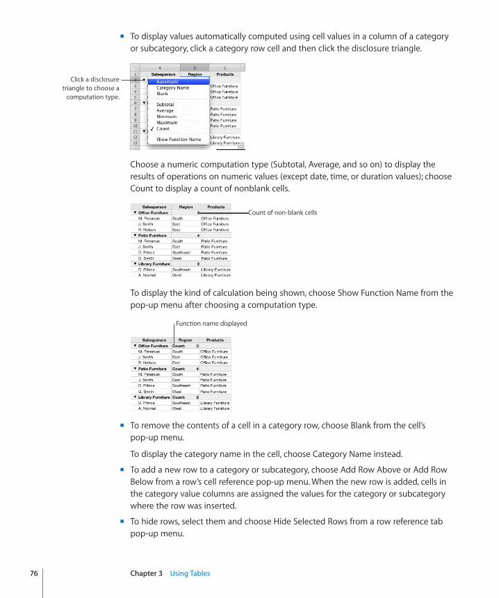
To display values automatically computed using cell values in a column of a category m
or subcategory, click a category row cell and then click the disclosure triangle.
Click a disclosure triangle to choose a
computation type.
Choose a numeric computation type (Subtotal, Average, and so on) to display the results of operations on numeric values (except date, time, or duration values); choose Count to display a count of nonblank cells.
Count of non-blank cells
To display the kind of calculation being shown, choose Show Function Name from the pop-up menu after choosing a computation type.
Function name displayed
To remove the contents of a cell in a category row, choose Blank from the cell’s m
pop-up menu.
To display the category name in the cell, choose Category Name instead.
To add a new row to a category or subcategory, choose Add Row Above or Add Row m
Below from a row’s cell reference pop-up menu. When the new row is added, cells in the category value columns are assigned the values for the category or subcategory where the row was inserted.
To hide rows, select them and choose Hide Selected Rows from a row reference tab m
pop-up menu.
76 Chapter 3 Using Tables
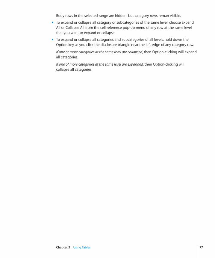
Chapter 3 Using Tables 77
Body rows in the selected range are hidden, but category rows reman visible.
To expand or collapse all category or subcategories of the same level, choose Expand m
All or Collapse All from the cell reference pop-up menu of any row at the same level that you want to expand or collapse.
To expand or collapse all categories and subcategories of all levels, hold down the m
Option key as you click the disclosure triangle near the left edge of any category row.
If one or more categories at the same level are collapsed, then Option-clicking will expand all categories.
If one of more categories at the same level are expanded, then Option-clicking will collapse all categories.
78
This chapter describes how to work with table cells and their content.
Putting Content into Table CellsUse a variety of techniques to add content to table cells.
To learn how to Go to
Add, replace, copy, paste, and move table cell values
“Adding and Editing Table Cell Values” on page 78
Format and align text in table cells and use find-and-replace and spell-checking features
“Working with Text in Table Cells” on page 79
Work with numeric table cell values “Working with Numbers in Table Cells” on page 80
Use autofilling to automatically repeat a cell value in adjacent cells
“Autofilling Table Cells” on page 81
Adding and Editing Table Cell ValuesYou can add, change, and delete the content in cells.
Here are ways to add and edit values:�If the cell is empty, select it and then type a value. “ m Selecting a Table Cell” on page 55 describes how to select cells.
To replace specific content already in the cell, select the cell and then select what you m
want to replace by double-clicking; hold down the Shift key and select more content if you want to replace more. Type to replace the selected content.
To replace everything in the cell, select the cell and then begin typing. m
If “Return key moves to next cell” isn’t selected in the Table inspector, you can also select the cell and then press Return or Enter, which selects everything in the cell, and then start typing.
4Working with Table Cells
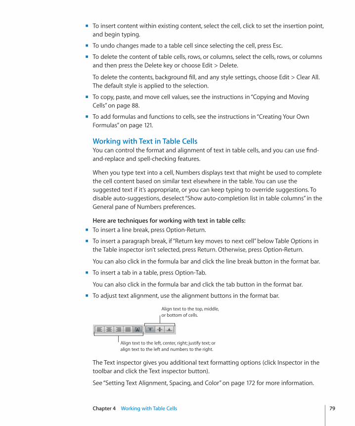
Chapter 4 Working with Table Cells 79
To insert content within existing content, select the cell, click to set the insertion point, m
and begin typing.
To undo changes made to a table cell since selecting the cell, press Esc. m
To delete the content of table cells, rows, or columns, select the cells, rows, or columns m
and then press the Delete key or choose Edit > Delete.
To delete the contents, background fill, and any style settings, choose Edit > Clear All. The default style is applied to the selection.
To copy, paste, and move cell values, see the instructions in “ m Copying and Moving Cells” on page 88.
To add formulas and functions to cells, see the instructions in “ m Creating Your Own Formulas” on page 121.
Working with Text in Table CellsYou can control the format and alignment of text in table cells, and you can use find-and-replace and spell-checking features.
When you type text into a cell, Numbers displays text that might be used to complete the cell content based on similar text elsewhere in the table. You can use the suggested text if it’s appropriate, or you can keep typing to override suggestions. To disable auto-suggestions, deselect “Show auto-completion list in table columns” in the General pane of Numbers preferences.
Here are techniques for working with text in table cells:�To insert a line break, press Option-Return. m
To insert a paragraph break, if “Return key moves to next cell” below Table Options in m
the Table inspector isn’t selected, press Return. Otherwise, press Option-Return.
You can also click in the formula bar and click the line break button in the format bar.
To insert a tab in a table, press Option-Tab. m
You can also click in the formula bar and click the tab button in the format bar.
To adjust text alignment, use the alignment buttons in the format bar. m
Align text to the left, center, right; justify text; or align text to the left and numbers to the right.
Align text to the top, middle, or bottom of cells.
The Text inspector gives you additional text formatting options (click Inspector in the toolbar and click the Text inspector button).
See “Setting Text Alignment, Spacing, and Color” on page 172 for more information.
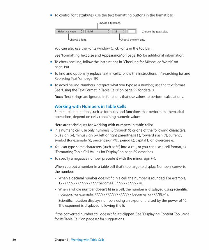
To control font attributes, use the text formatting buttons in the format bar. m
Choose a font.
Choose a typeface.
Choose the font size.
Choose the text color.
You can also use the Fonts window (click Fonts in the toolbar).
See “Formatting Text Size and Appearance” on page 165 for additional information.
To check spelling, follow the instructions in “ m Checking for Misspelled Words” on page 190.
To find and optionally replace text in cells, follow the instructions in “ m Searching for and Replacing Text” on page 192.
To avoid having Numbers interpret what you type as a number, use the text format. m
See “Using the Text Format in Table Cells” on page 99 for details.
Note: Text strings are ignored in functions that use values to perform calculations.
Working with Numbers in Table CellsSome table operations, such as formulas and functions that perform mathematical operations, depend on cells containing numeric values.
Here are techniques for working with numbers in table cells:�In a numeric cell use only numbers (0 through 9) or one of the following characters: m
plus sign (+), minus sign (–), left or right parenthesis ( ), forward slash (/), currency symbol (for example, $), percent sign (%), period (.), capital E, or lowercase e.
You can type some characters (such as %) into a cell, or you can use a cell format, as m
“Formatting Table Cell Values for Display” on page 89 describes.
To specify a negative number, precede it with the minus sign (–). m
When you put a number in a table cell that’s too large to display, Numbers converts the number:
When a decimal number doesn’t fit in a cell, the number is rounded. For example, Â1.77777777777777777777 becomes 1.77777777777778.
When a whole number doesn’t fit in a cell, the number is displayed using scientific Ânotation. For example, 77777777777777777777 becomes 7.777778E+19.
Scientific notation displays numbers using an exponent raised by the power of 10. The exponent is displayed following the E.
If the converted number still doesn’t fit, it’s clipped. See “Displaying Content Too Large for Its Table Cell” on page 82 for suggestions.
80 Chapter 4 Working with Table Cells
Chapter 4 Working with Table Cells 81
Instructions for using formulas and functions in table cells are in “Creating Your Own Formulas” on page 121.
Autofilling Table CellsWith autofilling you can use the content in one or more cells to automatically add values to adjacent cells.
Here are ways to autofill table cells:To paste the content and fill of a cell into adjacent cells, select the cell and then drag m
the Fill handle (a small circle in the cell’s lower-right corner) over the cells into which you want to paste.
Any data, cell format, formula, or fill associated with the selected cell is pasted, but comments aren’t pasted. If any target cell contains data, autofilling overwrites that data with the value you’re repeating.
To paste the content and fill of a cell into one or more cells in the same row or column, m
select two or more adjacent cells and choose one of the following:
Insert > Fill > Fill Right:� Assigns selected cells the value in the leftmost selected cell.
Insert > Fill > Fill Left:� Assigns selected cells the value in the rightmost selected cell.
Insert > Fill > Fill Up:� Assigns selected cells the value in the bottommost selected cell.
Insert > Fill > Fill Down:� Assigns selected cells the value in the topmost selected cell.
Any data, cell format, formula, or fill associated with the selected cell is pasted, but comments aren’t pasted. If any target cell contains data, autofilling overwrites that data with the value you’re repeating.
You can also add values to cells based on value patterns. For example, if a cell contains m
a day of the week or a month, you can select the cell and then drag to the right or down to add the next day of the week or month to the adjacent cell.
To create new values based on numeric patterns, select two or more cells before dragging. For example, if two selected cells contain 1 and 2, the values 3 and 4 are added when you drag through the adjacent two cells. And if two selected cells contain 1 and 4, the values 7 and 10 are added when you drag through the adjacent two cells (values are incremented by 3).
Autofilling doesn’t set up an ongoing relationship among cells in the group. After autofilling, you can change the cells independently of each other.
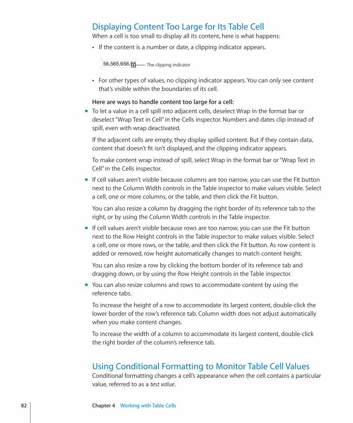
Displaying Content Too Large for Its Table CellWhen a cell is too small to display all its content, here is what happens:
If the content is a number or date, a clipping indicator appears. Â
The clipping indicator
For other types of values, no clipping indicator appears. You can only see content Âthat’s visible within the boundaries of its cell.
Here are ways to handle content too large for a cell:�To let a value in a cell spill into adjacent cells, deselect Wrap in the format bar or m
deselect “Wrap Text in Cell” in the Cells inspector. Numbers and dates clip instead of spill, even with wrap deactivated.
If the adjacent cells are empty, they display spilled content. But if they contain data, content that doesn’t fit isn’t displayed, and the clipping indicator appears.
To make content wrap instead of spill, select Wrap in the format bar or “Wrap Text in Cell” in the Cells inspector.
If cell values aren’t visible because columns are too narrow, you can use the Fit button m
next to the Column Width controls in the Table inspector to make values visible. Select a cell, one or more columns, or the table, and then click the Fit button.
You can also resize a column by dragging the right border of its reference tab to the right, or by using the Column Width controls in the Table inspector.
If cell values aren’t visible because rows are too narrow, you can use the Fit button m
next to the Row Height controls in the Table inspector to make values visible. Select a cell, one or more rows, or the table, and then click the Fit button. As row content is added or removed, row height automatically changes to match content height.
You can also resize a row by clicking the bottom border of its reference tab and dragging down, or by using the Row Height controls in the Table inspector.
You can also resize columns and rows to accommodate content by using the m
reference tabs.
To increase the height of a row to accommodate its largest content, double-click the lower border of the row’s reference tab. Column width does not adjust automatically when you make content changes.
To increase the width of a column to accommodate its largest content, double-click the right border of the column’s reference tab.
Using Conditional Formatting to Monitor Table Cell ValuesConditional formatting changes a cell’s appearance when the cell contains a particular value, referred to as a test value.
82 Chapter 4 Working with Table Cells
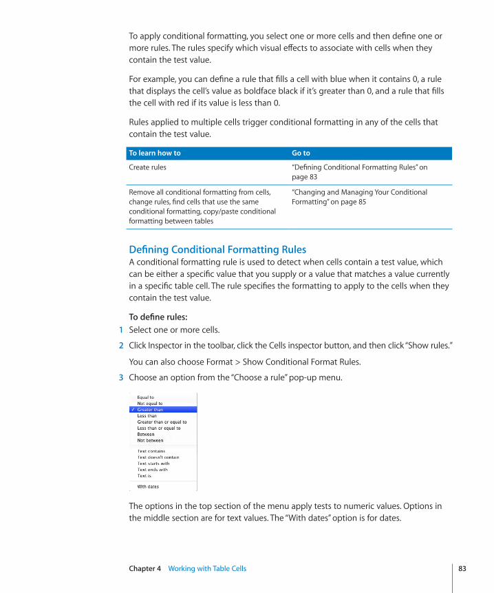
Chapter 4 Working with Table Cells 83
To apply conditional formatting, you select one or more cells and then define one or more rules. The rules specify which visual effects to associate with cells when they contain the test value.
For example, you can define a rule that fills a cell with blue when it contains 0, a rule that displays the cell’s value as boldface black if it’s greater than 0, and a rule that fills the cell with red if its value is less than 0.
Rules applied to multiple cells trigger conditional formatting in any of the cells that contain the test value.
To learn how to Go to
Create rules “Defining Conditional Formatting Rules” on page 83
Remove all conditional formatting from cells, change rules, find cells that use the same conditional formatting, copy/paste conditional formatting between tables
“Changing and Managing Your Conditional Formatting” on page 85
Defining Conditional Formatting RulesA conditional formatting rule is used to detect when cells contain a test value, which can be either a specific value that you supply or a value that matches a value currently in a specific table cell. The rule specifies the formatting to apply to the cells when they contain the test value.
To define rules: 1 Select one or more cells.
2 Click Inspector in the toolbar, click the Cells inspector button, and then click “Show rules.”
You can also choose Format > Show Conditional Format Rules.
3 Choose an option from the “Choose a rule” pop-up menu.
The options in the top section of the menu apply tests to numeric values. Options in the middle section are for text values. The “With dates” option is for dates.
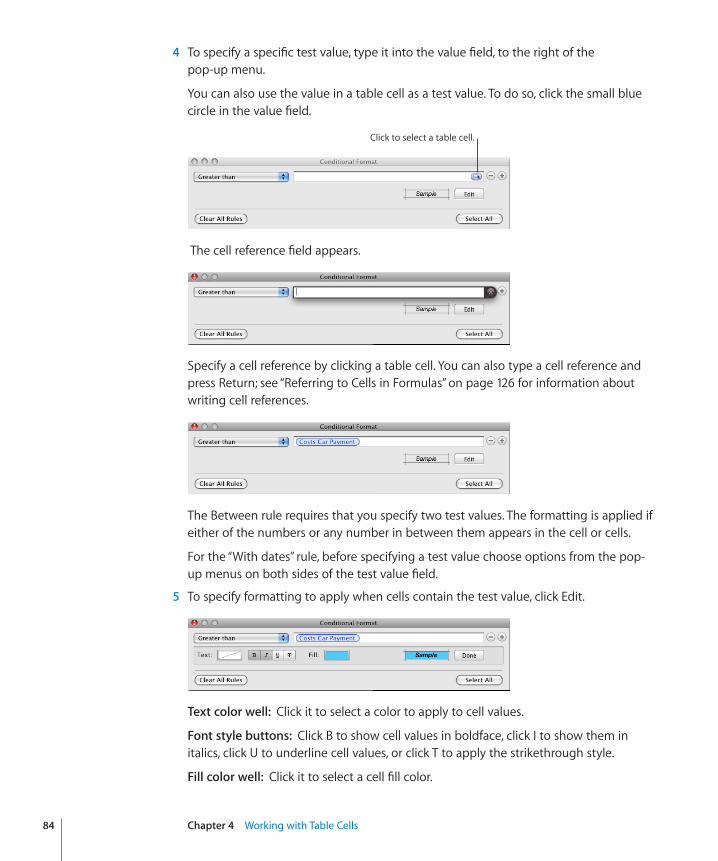
4 To specify a specific test value, type it into the value field, to the right of the pop-up menu.
You can also use the value in a table cell as a test value. To do so, click the small blue circle in the value field.
Click to select a table cell.
The cell reference field appears.
Specify a cell reference by clicking a table cell. You can also type a cell reference and press Return; see “Referring to Cells in Formulas” on page 126 for information about writing cell references.
The Between rule requires that you specify two test values. The formatting is applied if either of the numbers or any number in between them appears in the cell or cells.
For the “With dates” rule, before specifying a test value choose options from the pop-up menus on both sides of the test value field.
5 To specify formatting to apply when cells contain the test value, click Edit.
Text color well:� Click it to select a color to apply to cell values.
Font style buttons:� Click B to show cell values in boldface, click I to show them in italics, click U to underline cell values, or click T to apply the strikethrough style.
Fill color well:� Click it to select a cell fill color.
84 Chapter 4 Working with Table Cells
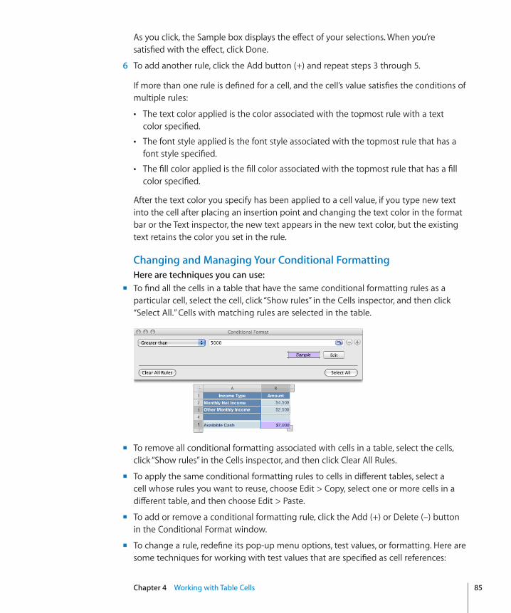
Chapter 4 Working with Table Cells 85
As you click, the Sample box displays the effect of your selections. When you’re satisfied with the effect, click Done.
6 To add another rule, click the Add button (+) and repeat steps 3 through 5.
If more than one rule is defined for a cell, and the cell’s value satisfies the conditions of multiple rules:
The text color applied is the color associated with the topmost rule with a text Âcolor specified.
The font style applied is the font style associated with the topmost rule that has a Âfont style specified.
The fill color applied is the fill color associated with the topmost rule that has a fill Âcolor specified.
After the text color you specify has been applied to a cell value, if you type new text into the cell after placing an insertion point and changing the text color in the format bar or the Text inspector, the new text appears in the new text color, but the existing text retains the color you set in the rule.
Changing and Managing Your Conditional FormattingHere are techniques you can use:� To find all the cells in a table that have the same conditional formatting rules as a m
particular cell, select the cell, click “Show rules” in the Cells inspector, and then click “Select All.” Cells with matching rules are selected in the table.
To remove all conditional formatting associated with cells in a table, select the cells, m
click “Show rules” in the Cells inspector, and then click Clear All Rules.
To apply the same conditional formatting rules to cells in different tables, select a m
cell whose rules you want to reuse, choose Edit > Copy, select one or more cells in a different table, and then choose Edit > Paste.
To add or remove a conditional formatting rule, click the Add (+) or Delete (–) button m
in the Conditional Format window.
To change a rule, redefine its pop-up menu options, test values, or formatting. Here are m
some techniques for working with test values that are specified as cell references:
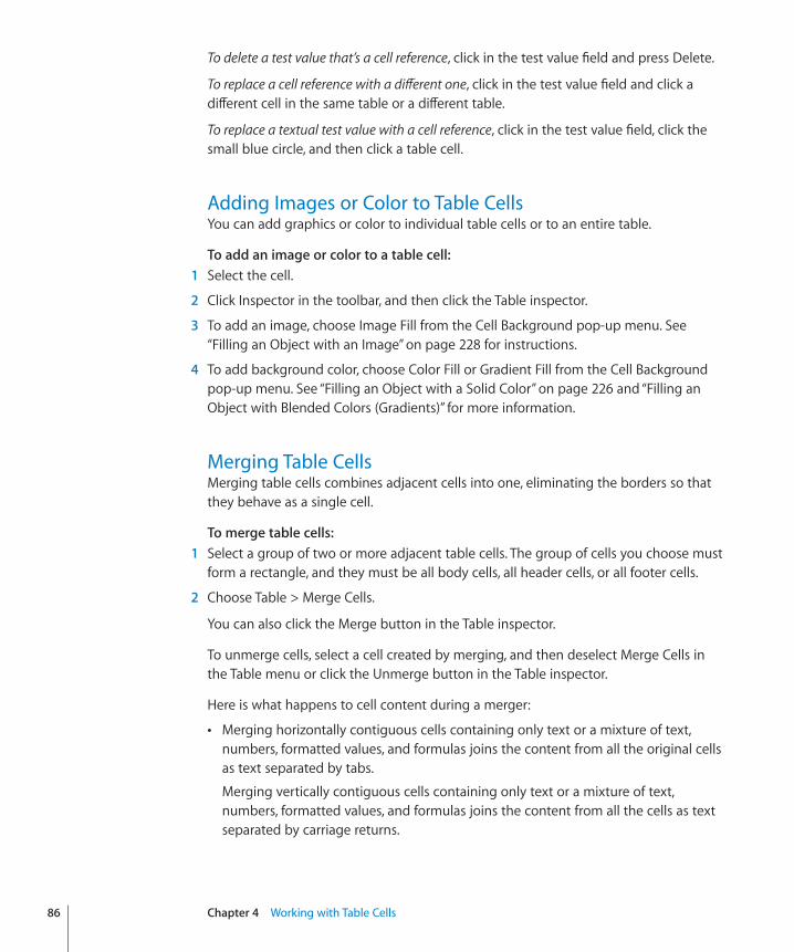
To delete a test value that’s a cell reference, click in the test value field and press Delete.
To replace a cell reference with a different one, click in the test value field and click a different cell in the same table or a different table.
To replace a textual test value with a cell reference, click in the test value field, click the small blue circle, and then click a table cell.
Adding Images or Color to Table CellsYou can add graphics or color to individual table cells or to an entire table.
To add an image or color to a table cell:� 1 Select the cell.
2 Click Inspector in the toolbar, and then click the Table inspector.
3 To add an image, choose Image Fill from the Cell Background pop-up menu. See “Filling an Object with an Image” on page 228 for instructions.
4 To add background color, choose Color Fill or Gradient Fill from the Cell Background pop-up menu. See “Filling an Object with a Solid Color” on page 226 and “Filling an Object with Blended Colors (Gradients)” for more information.
Merging Table CellsMerging table cells combines adjacent cells into one, eliminating the borders so that they behave as a single cell.
To merge table cells:� 1 Select a group of two or more adjacent table cells. The group of cells you choose must
form a rectangle, and they must be all body cells, all header cells, or all footer cells.
2 Choose Table > Merge Cells.
You can also click the Merge button in the Table inspector.
To unmerge cells, select a cell created by merging, and then deselect Merge Cells in the Table menu or click the Unmerge button in the Table inspector.
Here is what happens to cell content during a merger:
Merging horizontally contiguous cells containing only text or a mixture of text, Ânumbers, formatted values, and formulas joins the content from all the original cells as text separated by tabs.
Merging vertically contiguous cells containing only text or a mixture of text, numbers, formatted values, and formulas joins the content from all the cells as text separated by carriage returns.
86 Chapter 4 Working with Table Cells
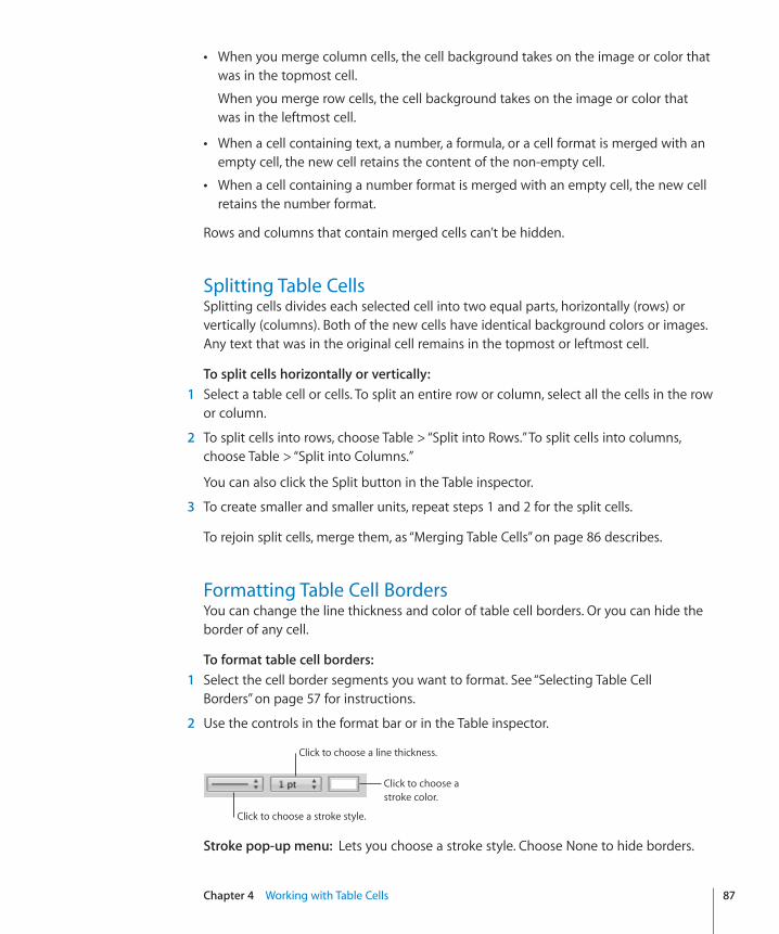
Chapter 4 Working with Table Cells 87
When you merge column cells, the cell background takes on the image or color that Âwas in the topmost cell.
When you merge row cells, the cell background takes on the image or color that was in the leftmost cell.
When a cell containing text, a number, a formula, or a cell format is merged with an Âempty cell, the new cell retains the content of the non-empty cell.
When a cell containing a number format is merged with an empty cell, the new cell Âretains the number format.
Rows and columns that contain merged cells can’t be hidden.
Splitting Table CellsSplitting cells divides each selected cell into two equal parts, horizontally (rows) or vertically (columns). Both of the new cells have identical background colors or images. Any text that was in the original cell remains in the topmost or leftmost cell.
To split cells horizontally or vertically:� 1 Select a table cell or cells. To split an entire row or column, select all the cells in the row
or column.
2 To split cells into rows, choose Table > “Split into Rows.” To split cells into columns, choose Table > “Split into Columns.”
You can also click the Split button in the Table inspector.
3 To create smaller and smaller units, repeat steps 1 and 2 for the split cells.
To rejoin split cells, merge them, as “Merging Table Cells” on page 86 describes.
Formatting Table Cell BordersYou can change the line thickness and color of table cell borders. Or you can hide the border of any cell.
To format table cell borders:� 1 Select the cell border segments you want to format. See “Selecting Table Cell
Borders” on page 57 for instructions.
2 Use the controls in the format bar or in the Table inspector.
Click to choose a stroke color.
Click to choose a stroke style.
Click to choose a line thickness.
Stroke pop-up menu:� Lets you choose a stroke style. Choose None to hide borders.
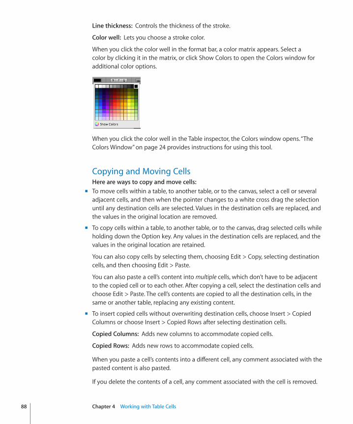
Line thickness:� Controls the thickness of the stroke.
Color well:� Lets you choose a stroke color.
When you click the color well in the format bar, a color matrix appears. Select a color by clicking it in the matrix, or click Show Colors to open the Colors window for additional color options.
When you click the color well in the Table inspector, the Colors window opens. “The Colors Window” on page 24 provides instructions for using this tool.
Copying and Moving CellsHere are ways to copy and move cells:�To move cells within a table, to another table, or to the canvas, select a cell or several m
adjacent cells, and then when the pointer changes to a white cross drag the selection until any destination cells are selected. Values in the destination cells are replaced, and the values in the original location are removed.
To copy cells within a table, to another table, or to the canvas, drag selected cells while m
holding down the Option key. Any values in the destination cells are replaced, and the values in the original location are retained.
You can also copy cells by selecting them, choosing Edit > Copy, selecting destination cells, and then choosing Edit > Paste.
You can also paste a cell’s content into multiple cells, which don’t have to be adjacent to the copied cell or to each other. After copying a cell, select the destination cells and choose Edit > Paste. The cell’s contents are copied to all the destination cells, in the same or another table, replacing any existing content.
To insert copied cells without overwriting destination cells, choose Insert > Copied m
Columns or choose Insert > Copied Rows after selecting destination cells.
Copied Columns:� Adds new columns to accommodate copied cells.
Copied Rows:� Adds new rows to accommodate copied cells.
When you paste a cell’s contents into a different cell, any comment associated with the pasted content is also pasted.
If you delete the contents of a cell, any comment associated with the cell is removed.
88 Chapter 4 Working with Table Cells
Chapter 4 Working with Table Cells 89
See “Rearranging Rows and Columns” on page 61 to learn how to copy and move rows and columns using the reference tabs.
See “Copying or Moving Formulas and Their Computed Values” on page 131 to learn about techniques for duplicating or moving a cell that contains a formula.
Adding Comments to Table CellsUse comments to record information about table cells.
Here are ways to work with comments:�To add a comment to a cell, select the cell and click Comment in the toolbar, or choose m
Insert > Comment. Type in the comment box.
To move a comment, drag it. m
To hide all comments, choose View > Hide Comments. A yellow marker appears in any m
table cell containing a comment.
To hide one comment, click the Minimize (–) button in the upper left of the comment box, or click the comment marker. A hidden comment can be temporarily displayed by placing the pointer over the marker.
To show all comments, choose View > Show Comments. m
To show a hidden comment, click its marker.
To delete a comment, click the X in the upper right of the comment box. m
To include comments when you print, show any comments you want to print, m
and then choose File > Print.
Formatting Table Cell Values for DisplayYou can apply a format to a cell to display its value in a particular way. For example, you can apply the currency format to cells that hold monetary values so that a currency symbol (such as $, £, or ¥) appears in front of numbers in the cells.
When you use a cell format, you are setting only the display characteristics of a value. When the value is used in formulas, the actual value is used, not the formatted value. The only exception is when there are too many numbers following a decimal point, in which case the number is rounded.
Here are ways to work with cell formats:�You apply cell formats by selecting one or more cells and then using the format bar or m
the Cell Format pop-up menu in the Cells inspector to select the format.
To add a value to an empty cell that has a format, select the cell and enter a value. m
The format is applied when you leave the cell.
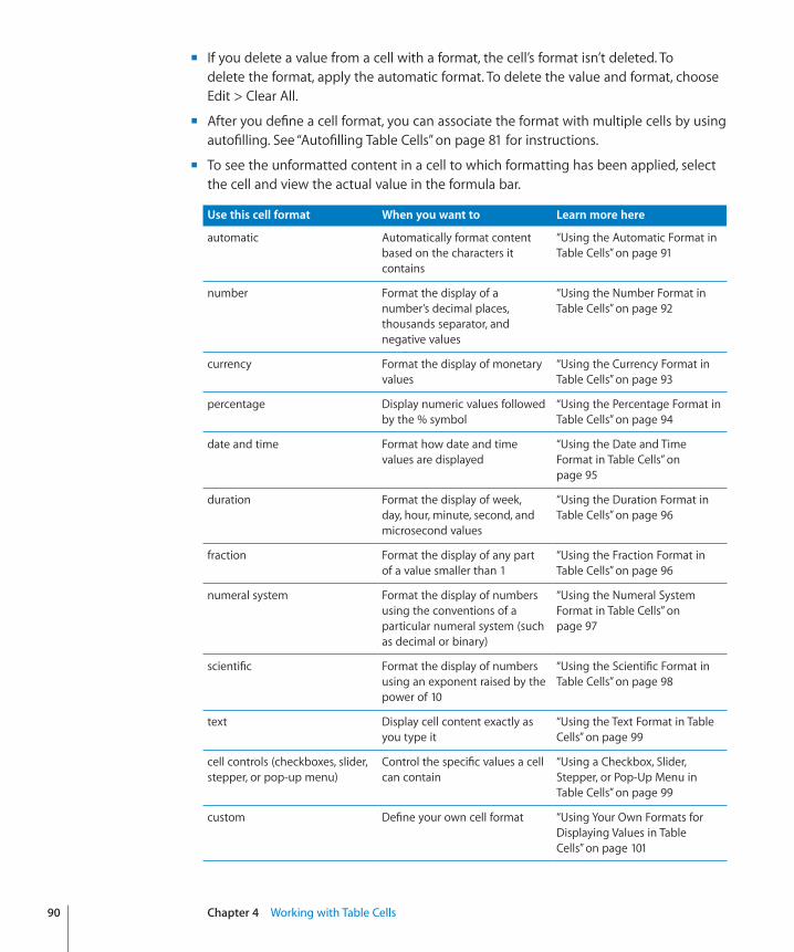
If you delete a value from a cell with a format, the cell’s format isn’t deleted. To m
delete the format, apply the automatic format. To delete the value and format, choose Edit > Clear All.
After you define a cell format, you can associate the format with multiple cells by using m
autofilling. See “Autofilling Table Cells” on page 81 for instructions.
To see the unformatted content in a cell to which formatting has been applied, select m
the cell and view the actual value in the formula bar.
Use this cell format When you want to Learn more here
automatic Automatically format content based on the characters it contains
“Using the Automatic Format in Table Cells” on page 91
number Format the display of a number’s decimal places, thousands separator, and negative values
“Using the Number Format in Table Cells” on page 92
currency Format the display of monetary values
“Using the Currency Format in Table Cells” on page 93
percentage Display numeric values followed by the % symbol
“Using the Percentage Format in Table Cells” on page 94
date and time Format how date and time values are displayed
“Using the Date and Time Format in Table Cells” on page 95
duration Format the display of week, day, hour, minute, second, and microsecond values
“Using the Duration Format in Table Cells” on page 96
fraction Format the display of any part of a value smaller than 1
“Using the Fraction Format in Table Cells” on page 96
numeral system Format the display of numbers using the conventions of a particular numeral system (such as decimal or binary)
“Using the Numeral System Format in Table Cells” on page 97
scientific Format the display of numbers using an exponent raised by the power of 10
“Using the Scientific Format in Table Cells” on page 98
text Display cell content exactly as you type it
“Using the Text Format in Table Cells” on page 99
cell controls (checkboxes, slider, stepper, or pop-up menu)
Control the specific values a cell can contain
“Using a Checkbox, Slider, Stepper, or Pop-Up Menu in Table Cells” on page 99
custom Define your own cell format “Using Your Own Formats for Displaying Values in Table Cells” on page 101
90 Chapter 4 Working with Table Cells
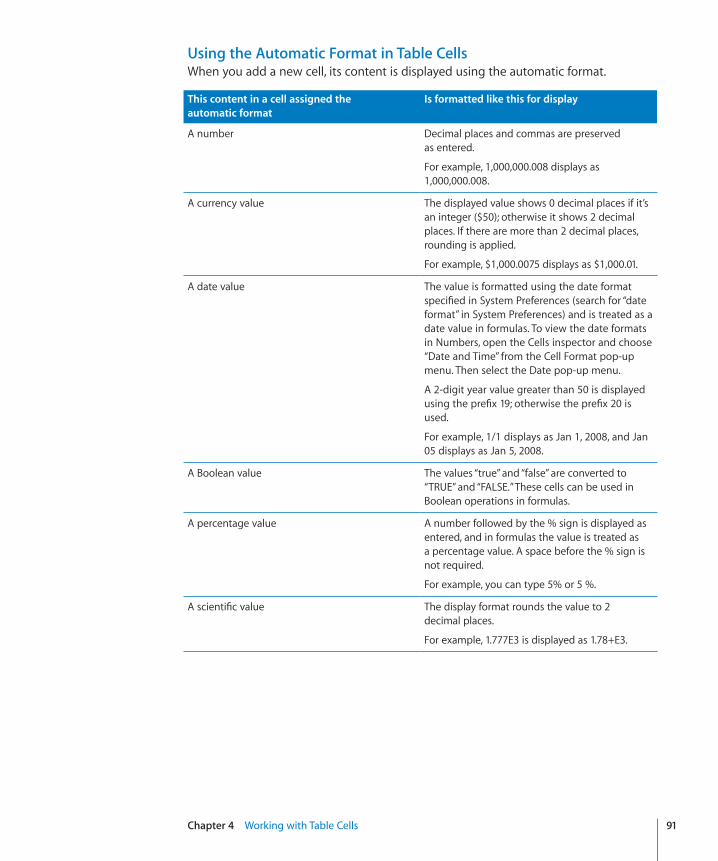
Chapter 4 Working with Table Cells 91
Using the Automatic Format in Table CellsWhen you add a new cell, its content is displayed using the automatic format.
This content in a cell assigned the automatic format
Is formatted like this for display
A number Decimal places and commas are preserved as entered.
For example, 1,000,000.008 displays as 1,000,000.008.
A currency value The displayed value shows 0 decimal places if it’s an integer ($50); otherwise it shows 2 decimal places. If there are more than 2 decimal places, rounding is applied.
For example, $1,000.0075 displays as $1,000.01.
A date value The value is formatted using the date format specified in System Preferences (search for “date format” in System Preferences) and is treated as a date value in formulas. To view the date formats in Numbers, open the Cells inspector and choose “Date and Time” from the Cell Format pop-up menu. Then select the Date pop-up menu.
A 2-digit year value greater than 50 is displayed using the prefix 19; otherwise the prefix 20 is used.
For example, 1/1 displays as Jan 1, 2008, and Jan 05 displays as Jan 5, 2008.
A Boolean value The values “true” and “false” are converted to “TRUE” and “FALSE.” These cells can be used in Boolean operations in formulas.
A percentage value A number followed by the % sign is displayed as entered, and in formulas the value is treated as a percentage value. A space before the % sign is not required.
For example, you can type 5% or 5 %.
A scientific value The display format rounds the value to 2 decimal places.
For example, 1.777E3 is displayed as 1.78+E3.
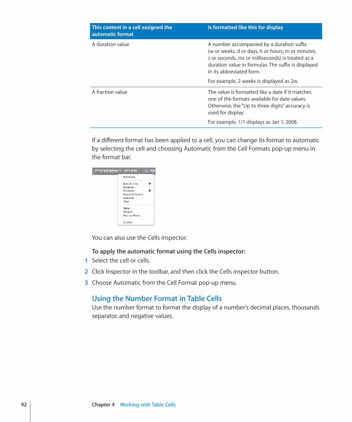
This content in a cell assigned the automatic format
Is formatted like this for display
A duration value A number accompanied by a duration suffix (w or weeks, d or days, h or hours, m or minutes, s or seconds, ms or milliseconds) is treated as a duration value in formulas. The suffix is displayed in its abbreviated form.
For example, 2 weeks is displayed as 2w.
A fraction value The value is formatted like a date if it matches one of the formats available for date values. Otherwise, the “Up to three digits” accuracy is used for display.
For example, 1/1 displays as Jan 1, 2008.
If a different format has been applied to a cell, you can change its format to automatic by selecting the cell and choosing Automatic from the Cell Formats pop-up menu in the format bar.
You can also use the Cells inspector.
To apply the automatic format using the Cells inspector:� 1 Select the cell or cells.
2 Click Inspector in the toolbar, and then click the Cells inspector button.
3 Choose Automatic from the Cell Format pop-up menu.
Using the Number Format in Table CellsUse the number format to format the display of a number’s decimal places, thousands separator, and negative values.
92 Chapter 4 Working with Table Cells
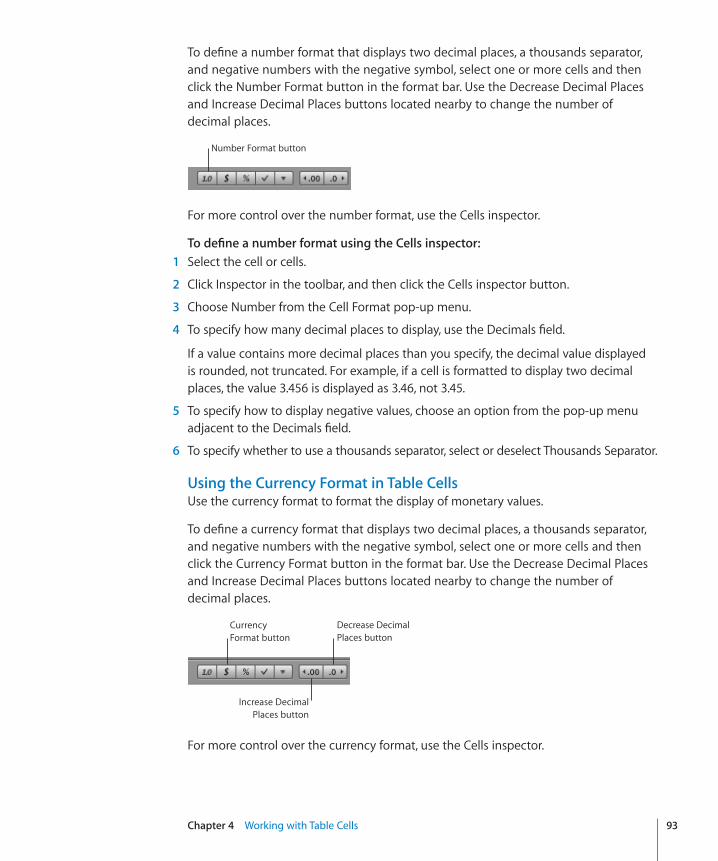
Chapter 4 Working with Table Cells 93
To define a number format that displays two decimal places, a thousands separator, and negative numbers with the negative symbol, select one or more cells and then click the Number Format button in the format bar. Use the Decrease Decimal Places and Increase Decimal Places buttons located nearby to change the number of decimal places.
Number Format button
For more control over the number format, use the Cells inspector.
To define a number format using the Cells inspector: 1 Select the cell or cells.
2 Click Inspector in the toolbar, and then click the Cells inspector button.
3 Choose Number from the Cell Format pop-up menu.
4 To specify how many decimal places to display, use the Decimals field.
If a value contains more decimal places than you specify, the decimal value displayed is rounded, not truncated. For example, if a cell is formatted to display two decimal places, the value 3.456 is displayed as 3.46, not 3.45.
5 To specify how to display negative values, choose an option from the pop-up menu adjacent to the Decimals field.
6 To specify whether to use a thousands separator, select or deselect Thousands Separator.
Using the Currency Format in Table CellsUse the currency format to format the display of monetary values.
To define a currency format that displays two decimal places, a thousands separator, and negative numbers with the negative symbol, select one or more cells and then click the Currency Format button in the format bar. Use the Decrease Decimal Places and Increase Decimal Places buttons located nearby to change the number of decimal places.
Increase Decimal Places button
Decrease Decimal Places button
Currency Format button
For more control over the currency format, use the Cells inspector.
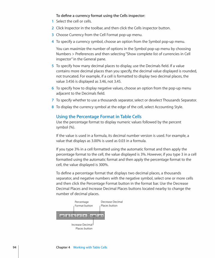
To define a currency format using the Cells inspector: 1 Select the cell or cells.
2 Click Inspector in the toolbar, and then click the Cells inspector button.
3 Choose Currency from the Cell Format pop-up menu.
4 To specify a currency symbol, choose an option from the Symbol pop-up menu.
You can maximize the number of options in the Symbol pop-up menu by choosing Numbers > Preferences and then selecting “Show complete list of currencies in Cell inspector” in the General pane.
5 To specify how many decimal places to display, use the Decimals field. If a value contains more decimal places than you specify, the decimal value displayed is rounded, not truncated. For example, if a cell is formatted to display two decimal places, the value 3.456 is displayed as 3.46, not 3.45.
6 To specify how to display negative values, choose an option from the pop-up menu adjacent to the Decimals field.
7 To specify whether to use a thousands separator, select or deselect Thousands Separator.
8 To display the currency symbol at the edge of the cell, select Accounting Style.
Using the Percentage Format in Table CellsUse the percentage format to display numeric values followed by the percent symbol (%).
If the value is used in a formula, its decimal number version is used. For example, a value that displays as 3.00% is used as 0.03 in a formula.
If you type 3% in a cell formatted using the automatic format and then apply the percentage format to the cell, the value displayed is 3%. However, if you type 3 in a cell formatted using the automatic format and then apply the percentage format to the cell, the value displayed is 300%.
To define a percentage format that displays two decimal places, a thousands separator, and negative numbers with the negative symbol, select one or more cells and then click the Percentage Format button in the format bar. Use the Decrease Decimal Places and Increase Decimal Places buttons located nearby to change the number of decimal places.
Increase Decimal Places button
Decrease Decimal Places button
Percentage Format button
94 Chapter 4 Working with Table Cells
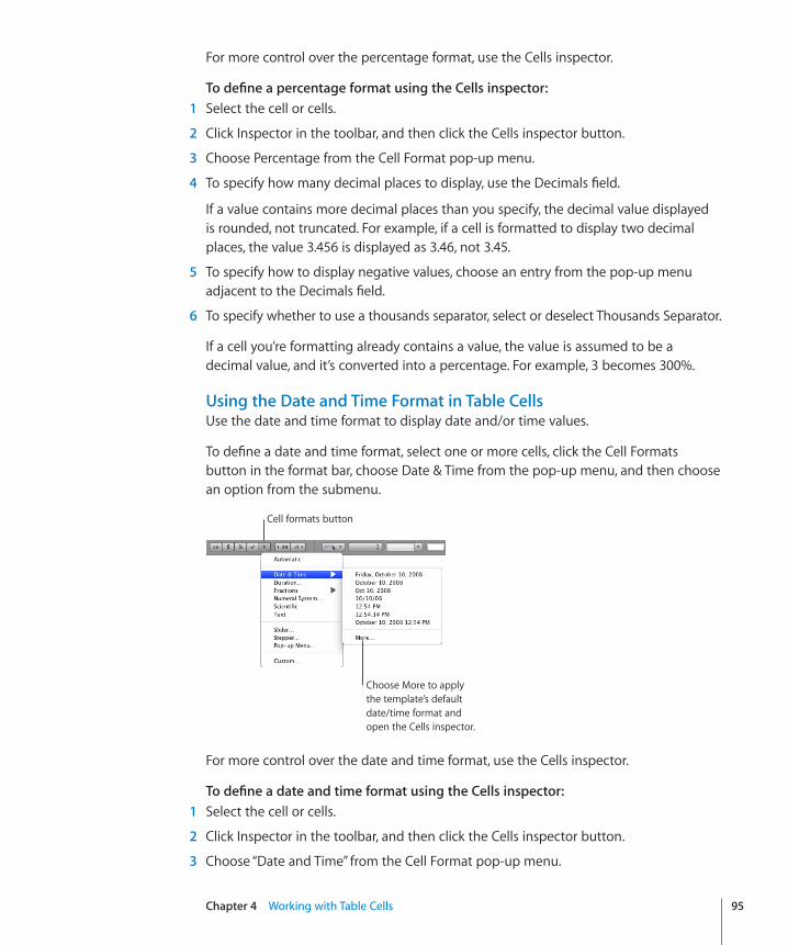
Chapter 4 Working with Table Cells 95
For more control over the percentage format, use the Cells inspector.
To define a percentage format using the Cells inspector: 1 Select the cell or cells.
2 Click Inspector in the toolbar, and then click the Cells inspector button.
3 Choose Percentage from the Cell Format pop-up menu.
4 To specify how many decimal places to display, use the Decimals field.
If a value contains more decimal places than you specify, the decimal value displayed is rounded, not truncated. For example, if a cell is formatted to display two decimal places, the value 3.456 is displayed as 3.46, not 3.45.
5 To specify how to display negative values, choose an entry from the pop-up menu adjacent to the Decimals field.
6 To specify whether to use a thousands separator, select or deselect Thousands Separator.
If a cell you’re formatting already contains a value, the value is assumed to be a decimal value, and it’s converted into a percentage. For example, 3 becomes 300%.
Using the Date and Time Format in Table CellsUse the date and time format to display date and/or time values.
To define a date and time format, select one or more cells, click the Cell Formats button in the format bar, choose Date & Time from the pop-up menu, and then choose an option from the submenu.
Cell formats button
Choose More to apply the template’s default date/time format and open the Cells inspector.
For more control over the date and time format, use the Cells inspector.
To define a date and time format using the Cells inspector: 1 Select the cell or cells.
2 Click Inspector in the toolbar, and then click the Cells inspector button.
3 Choose “Date and Time” from the Cell Format pop-up menu.
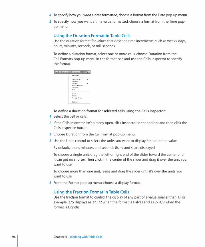
4 To specify how you want a date formatted, choose a format from the Date pop-up menu.
5 To specify how you want a time value formatted, choose a format from the Time pop-up menu.
Using the Duration Format in Table CellsUse the duration format for values that describe time increments, such as weeks, days, hours, minutes, seconds, or milliseconds.
To define a duration format, select one or more cells, choose Duration from the Cell Formats pop-up menu in the format bar, and use the Cells inspector to specify the format.
To define a duration format for selected cells using the Cells inspector: 1 Select the cell or cells.
2 If the Cells inspector isn’t already open, click Inspector in the toolbar and then click the Cells inspector button.
3 Choose Duration from the Cell Format pop-up menu.
4 Use the Units control to select the units you want to display for a duration value.
By default, hours, minutes, and seconds (h, m, and s) are displayed.
To choose a single unit, drag the left or right end of the slider toward the center until it can get no shorter. Then click in the center of the slider and drag it over the unit you want to use.
To choose more than one unit, resize and drag the slider until it’s over the units you want to use.
5 From the Format pop-up menu, choose a display format.
Using the Fraction Format in Table CellsUse the fraction format to control the display of any part of a value smaller than 1. For example, 27.5 displays as 27 1/2 when the format is Halves and as 27 4/8 when the format is Eighths.
96 Chapter 4 Working with Table Cells
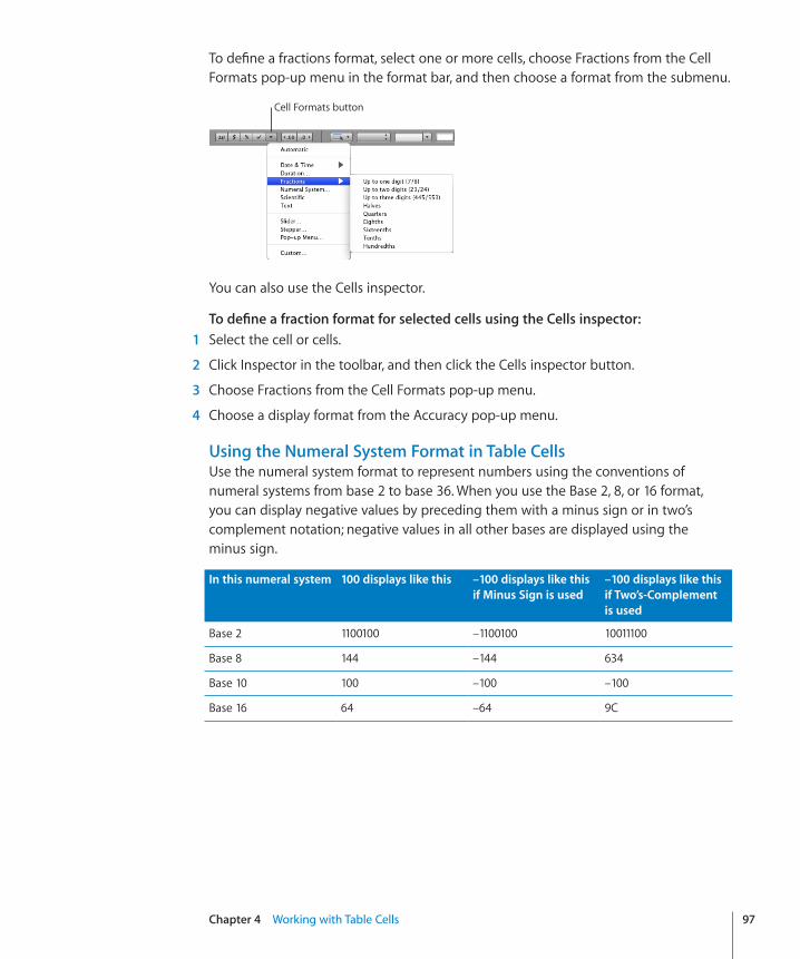
Chapter 4 Working with Table Cells 97
To define a fractions format, select one or more cells, choose Fractions from the Cell Formats pop-up menu in the format bar, and then choose a format from the submenu.
Cell Formats button
You can also use the Cells inspector.
To define a fraction format for selected cells using the Cells inspector: 1 Select the cell or cells.
2 Click Inspector in the toolbar, and then click the Cells inspector button.
3 Choose Fractions from the Cell Formats pop-up menu.
4 Choose a display format from the Accuracy pop-up menu.
Using the Numeral System Format in Table CellsUse the numeral system format to represent numbers using the conventions of numeral systems from base 2 to base 36. When you use the Base 2, 8, or 16 format, you can display negative values by preceding them with a minus sign or in two’s complement notation; negative values in all other bases are displayed using the minus sign.
In this numeral system 100 displays like this –100 displays like this if Minus Sign is used
–100 displays like this if Two’s-Complement is used
Base 2 1100100 –1100100 10011100
Base 8 144 –144 634
Base 10 100 –100 –100
Base 16 64 –64 9C
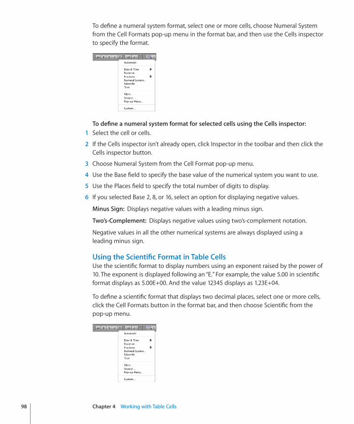
To define a numeral system format, select one or more cells, choose Numeral System from the Cell Formats pop-up menu in the format bar, and then use the Cells inspector to specify the format.
To define a numeral system format for selected cells using the Cells inspector: 1 Select the cell or cells.
2 If the Cells inspector isn’t already open, click Inspector in the toolbar and then click the Cells inspector button.
3 Choose Numeral System from the Cell Format pop-up menu.
4 Use the Base field to specify the base value of the numerical system you want to use.
5 Use the Places field to specify the total number of digits to display.
6 If you selected Base 2, 8, or 16, select an option for displaying negative values.
Minus Sign:� Displays negative values with a leading minus sign.
Two’s-Complement:� Displays negative values using two’s-complement notation.
Negative values in all the other numerical systems are always displayed using a leading minus sign.
Using the Scientific Format in Table CellsUse the scientific format to display numbers using an exponent raised by the power of 10. The exponent is displayed following an “E.” For example, the value 5.00 in scientific format displays as 5.00E+00. And the value 12345 displays as 1.23E+04.
To define a scientific format that displays two decimal places, select one or more cells, click the Cell Formats button in the format bar, and then choose Scientific from the pop-up menu.
98 Chapter 4 Working with Table Cells
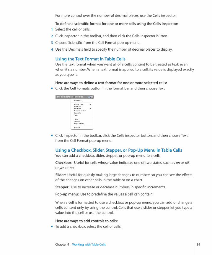
Chapter 4 Working with Table Cells 99
For more control over the number of decimal places, use the Cells inspector.
To define a scientific format for one or more cells using the Cells inspector: 1 Select the cell or cells.
2 Click Inspector in the toolbar, and then click the Cells inspector button.
3 Choose Scientific from the Cell Format pop-up menu.
4 Use the Decimals field to specify the number of decimal places to display.
Using the Text Format in Table CellsUse the text format when you want all of a cell’s content to be treated as text, even when it’s a number. When a text format is applied to a cell, its value is displayed exactly as you type it.
Here are ways to define a text format for one or more selected cells:Click the Cell Formats button in the format bar and then choose Text. m
Click Inspector in the toolbar, click the Cells inspector button, and then choose Text m
from the Cell Format pop-up menu.
Using a Checkbox, Slider, Stepper, or Pop-Up Menu in Table CellsYou can add a checkbox, slider, stepper, or pop-up menu to a cell:
Checkbox:� Useful for cells whose value indicates one of two states, such as on or off, or yes or no.
Slider:� Useful for quickly making large changes to numbers so you can see the effects of the changes on other cells in the table or on a chart.
Stepper:� Use to increase or decrease numbers in specific increments.
Pop-up menu:� Use to predefine the values a cell can contain.
When a cell is formatted to use a checkbox or pop-up menu, you can add or change a cell’s content only by using the control. Cells that use a slider or stepper let you type a value into the cell or use the control.
Here are ways to add controls to cells:�To add a checkbox, select the cell or cells. m
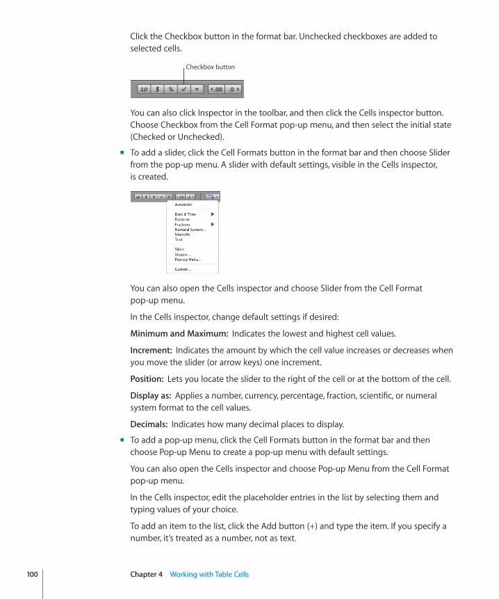
Click the Checkbox button in the format bar. Unchecked checkboxes are added to selected cells.
Checkbox button
You can also click Inspector in the toolbar, and then click the Cells inspector button. Choose Checkbox from the Cell Format pop-up menu, and then select the initial state (Checked or Unchecked).
To add a slider, click the Cell Formats button in the format bar and then choose Slider m
from the pop-up menu. A slider with default settings, visible in the Cells inspector, is created.
You can also open the Cells inspector and choose Slider from the Cell Format pop-up menu.
In the Cells inspector, change default settings if desired:
Minimum and Maximum:� Indicates the lowest and highest cell values.
Increment:� Indicates the amount by which the cell value increases or decreases when you move the slider (or arrow keys) one increment.
Position:� Lets you locate the slider to the right of the cell or at the bottom of the cell.
Display as:� Applies a number, currency, percentage, fraction, scientific, or numeral system format to the cell values.
Decimals:� Indicates how many decimal places to display.
To add a pop-up menu, click the Cell Formats button in the format bar and then m
choose Pop-up Menu to create a pop-up menu with default settings.
You can also open the Cells inspector and choose Pop-up Menu from the Cell Format pop-up menu.
In the Cells inspector, edit the placeholder entries in the list by selecting them and typing values of your choice.
To add an item to the list, click the Add button (+) and type the item. If you specify a number, it’s treated as a number, not as text.
100 Chapter 4 Working with Table Cells
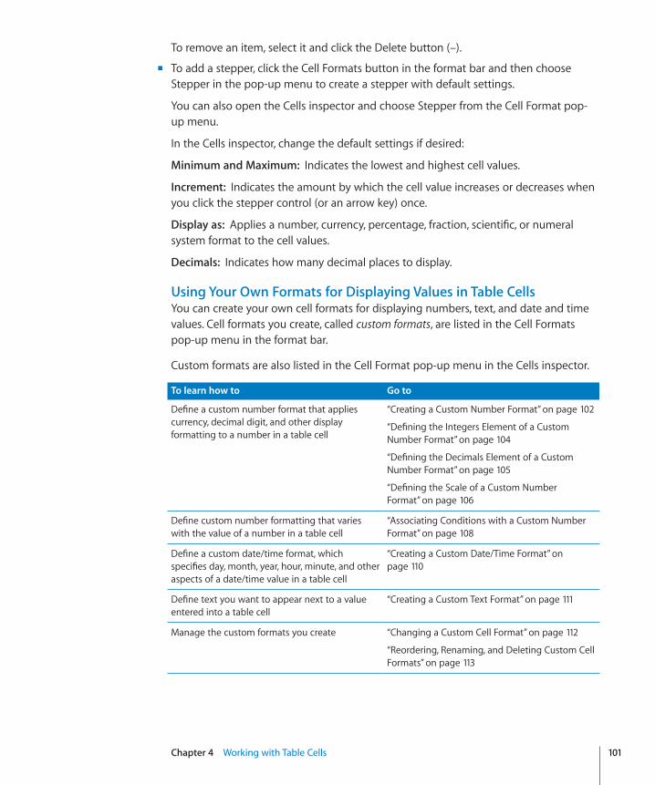
Chapter 4 Working with Table Cells 101
To remove an item, select it and click the Delete button (–).
To add a stepper, click the Cell Formats button in the format bar and then choose m
Stepper in the pop-up menu to create a stepper with default settings.
You can also open the Cells inspector and choose Stepper from the Cell Format pop-up menu.
In the Cells inspector, change the default settings if desired:
Minimum and Maximum:� Indicates the lowest and highest cell values.
Increment:� Indicates the amount by which the cell value increases or decreases when you click the stepper control (or an arrow key) once.
Display as:� Applies a number, currency, percentage, fraction, scientific, or numeral system format to the cell values.
Decimals:� Indicates how many decimal places to display.
Using Your Own Formats for Displaying Values in Table CellsYou can create your own cell formats for displaying numbers, text, and date and time values. Cell formats you create, called custom formats, are listed in the Cell Formats pop-up menu in the format bar.
Custom formats are also listed in the Cell Format pop-up menu in the Cells inspector.
To learn how to Go to
Define a custom number format that applies currency, decimal digit, and other display formatting to a number in a table cell
“Creating a Custom Number Format” on page 102
“Defining the Integers Element of a Custom Number Format” on page 104
“Defining the Decimals Element of a Custom Number Format” on page 105
“Defining the Scale of a Custom Number Format” on page 106
Define custom number formatting that varies with the value of a number in a table cell
“Associating Conditions with a Custom Number Format” on page 108
Define a custom date/time format, which specifies day, month, year, hour, minute, and other aspects of a date/time value in a table cell
“Creating a Custom Date/Time Format” on page 110
Define text you want to appear next to a value entered into a table cell
“Creating a Custom Text Format” on page 111
Manage the custom formats you create “Changing a Custom Cell Format” on page 112
“Reordering, Renaming, and Deleting Custom Cell Formats” on page 113
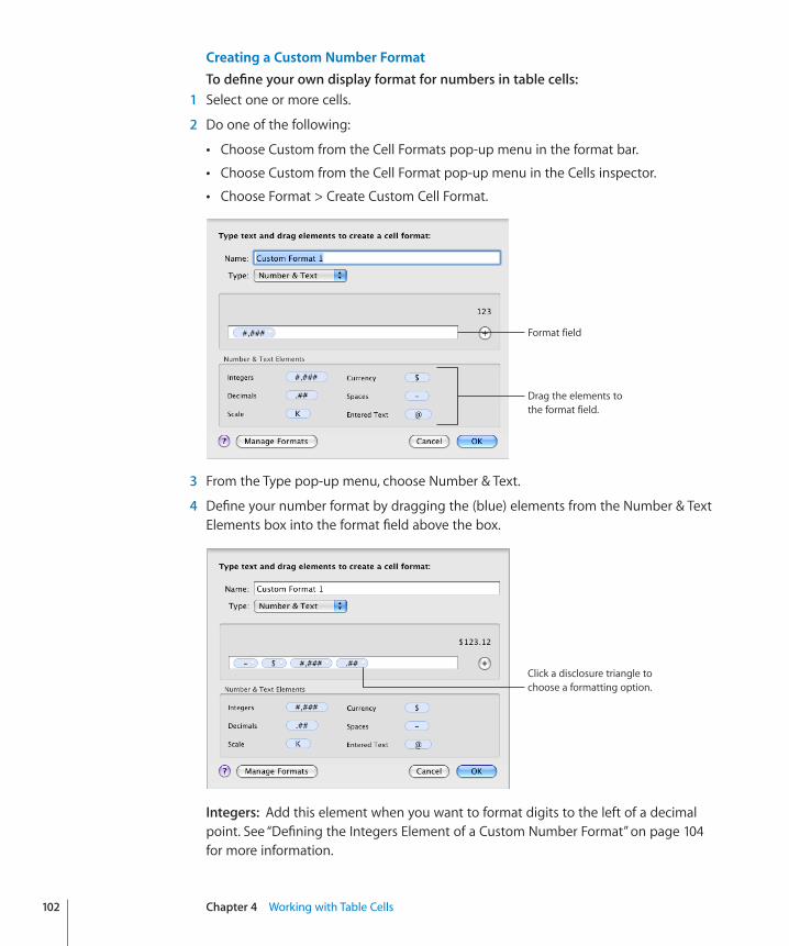
Creating a Custom Number FormatTo define your own display format for numbers in table cells:
1 Select one or more cells.
2 Do one of the following:
Choose Custom from the Cell Formats pop-up menu in the format bar. Â
Choose Custom from the Cell Format pop-up menu in the Cells inspector. Â
Choose Format > Create Custom Cell Format. Â
Format field
Drag the elements to the format field.
3 From the Type pop-up menu, choose Number & Text.
4 Define your number format by dragging the (blue) elements from the Number & Text Elements box into the format field above the box.
Click a disclosure triangle to choose a formatting option.
Integers:� Add this element when you want to format digits to the left of a decimal point. See “Defining the Integers Element of a Custom Number Format” on page 104 for more information.
102 Chapter 4 Working with Table Cells

Chapter 4 Working with Table Cells 103
Currency:� Add this element to display a currency symbol. To identify the symbol you want to use, click the disclosure triangle visible on the element when it’s in the format field and choose a symbol. You can maximize the choices in the pop-up menu by selecting “Show complete list of currencies in Cells inspector” in Numbers preferences.
Decimals:� Add this element to format how decimal digits are displayed. See “Defining the Decimals Element of a Custom Number Format” on page 105 for more information.
Spaces:� Use this element to control the amount of space displayed between elements. Click the disclosure triangle visible on the element when it’s in the format field and choose an option. Normal adds a standard space, Wide adds an em space, and Narrow adds a sixth of an em space. You can add more than one Spaces element to the format field with these options, but only one of the Spaces elements can be Flexible; this option left-aligns the elements that precede it and right-aligns elements that follow it.
Scale:� Use this element to size the display value of a number. For example, you can display values over 100 as number of hundreds (1000 displays as 10). See “Defining the Scale of a Custom Number Format” on page 106 for more information.
5 To display predefined text before or after any element, place an insertion point in the format field and then type your text. You can click any element and use the Left Arrow and Right Arrow keys to place the insertion point.
6 To delete an element in the field, select it and then press Delete.
To move the element around in the field, drag it.
7 In the Name field, type a name for your number format.
Custom format names are listed in the Cell Formats pop-up menu in the format bar and in the Cell Format pop-up menu of the Cells inspector.
8 Click OK to save your number format and apply it to the selected cells.
Here’s an example of a number format:
Balance:-$ #,### .##
The hyphen is a Spaces element, set to display one Normal space between the Âcurrency symbol and the number.
The dollar sign is a Currency element. Â
#,### is an Integers element that displays numbers greater than 999 with a Âthousands separator.
.## is a Decimals element. Â
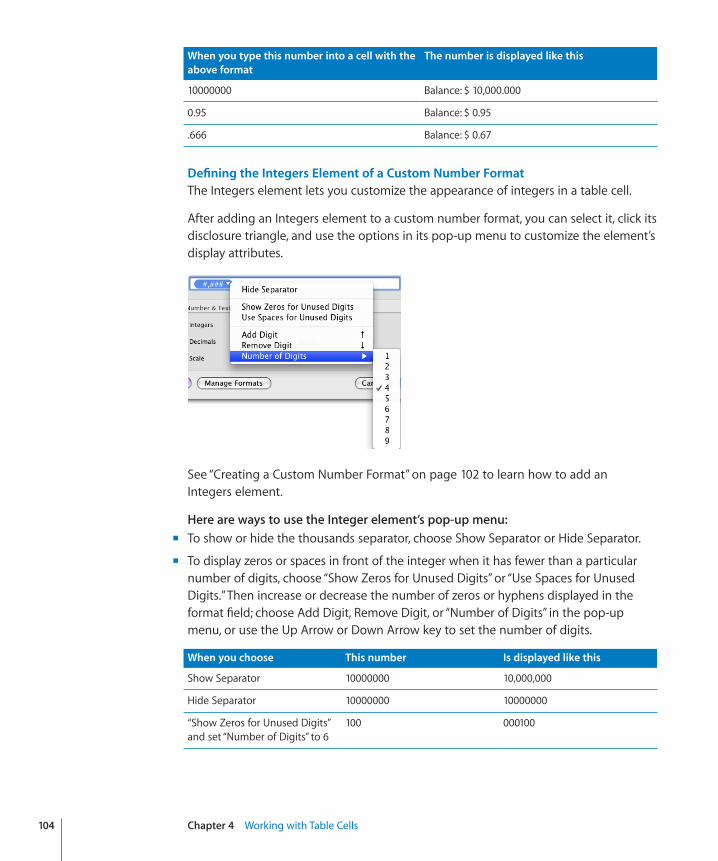
When you type this number into a cell with the above format
The number is displayed like this
10000000 Balance: $ 10,000.000
0.95 Balance: $ 0.95
.666 Balance: $ 0.67
Defining the Integers Element of a Custom Number FormatThe Integers element lets you customize the appearance of integers in a table cell.
After adding an Integers element to a custom number format, you can select it, click its disclosure triangle, and use the options in its pop-up menu to customize the element’s display attributes.
See “Creating a Custom Number Format” on page 102 to learn how to add an Integers element.
Here are ways to use the Integer element’s pop-up menu:�To show or hide the thousands separator, choose Show Separator or Hide Separator. m
To display zeros or spaces in front of the integer when it has fewer than a particular m
number of digits, choose “Show Zeros for Unused Digits” or “Use Spaces for Unused Digits.” Then increase or decrease the number of zeros or hyphens displayed in the format field; choose Add Digit, Remove Digit, or “Number of Digits” in the pop-up menu, or use the Up Arrow or Down Arrow key to set the number of digits.
When you choose This number Is displayed like this
Show Separator 10000000 10,000,000
Hide Separator 10000000 10000000
“Show Zeros for Unused Digits” and set “Number of Digits” to 6
100 000100
104 Chapter 4 Working with Table Cells
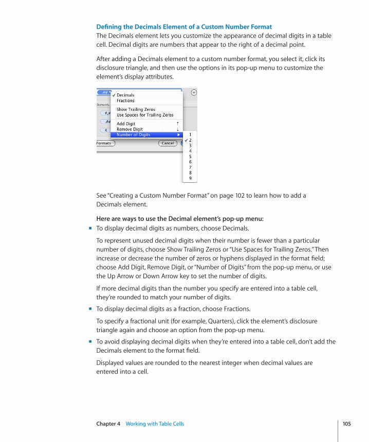
Chapter 4 Working with Table Cells 105
Defining the Decimals Element of a Custom Number FormatThe Decimals element lets you customize the appearance of decimal digits in a table cell. Decimal digits are numbers that appear to the right of a decimal point.
After adding a Decimals element to a custom number format, you select it, click its disclosure triangle, and then use the options in its pop-up menu to customize the element’s display attributes.
See “Creating a Custom Number Format” on page 102 to learn how to add a Decimals element.
Here are ways to use the Decimal element’s pop-up menu:�To display decimal digits as numbers, choose Decimals. m
To represent unused decimal digits when their number is fewer than a particular number of digits, choose Show Trailing Zeros or “Use Spaces for Trailing Zeros.” Then increase or decrease the number of zeros or hyphens displayed in the format field; choose Add Digit, Remove Digit, or “Number of Digits” from the pop-up menu, or use the Up Arrow or Down Arrow key to set the number of digits.
If more decimal digits than the number you specify are entered into a table cell, they’re rounded to match your number of digits.
To display decimal digits as a fraction, choose Fractions. m
To specify a fractional unit (for example, Quarters), click the element’s disclosure triangle again and choose an option from the pop-up menu.
To avoid displaying decimal digits when they’re entered into a table cell, don’t add the m
Decimals element to the format field.
Displayed values are rounded to the nearest integer when decimal values are entered into a cell.
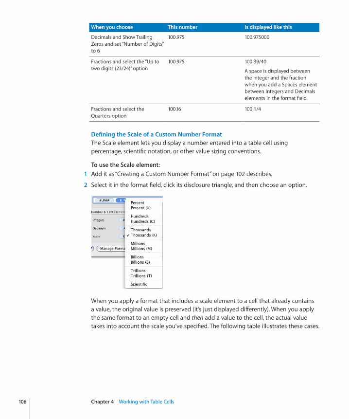
When you choose This number Is displayed like this
Decimals and Show Trailing Zeros and set “Number of Digits” to 6
100.975 100.975000
Fractions and select the “Up to two digits (23/24)” option
100.975 100 39/40
A space is displayed between the integer and the fraction when you add a Spaces element between Integers and Decimals elements in the format field.
Fractions and select the Quarters option
100.16 100 1/4
Defining the Scale of a Custom Number FormatThe Scale element lets you display a number entered into a table cell using percentage, scientific notation, or other value sizing conventions.
To use the Scale element:� 1 Add it as “Creating a Custom Number Format” on page 102 describes.
2 Select it in the format field, click its disclosure triangle, and then choose an option.
When you apply a format that includes a scale element to a cell that already contains a value, the original value is preserved (it’s just displayed differently). When you apply the same format to an empty cell and then add a value to the cell, the actual value takes into account the scale you’ve specified. The following table illustrates these cases.
106 Chapter 4 Working with Table Cells
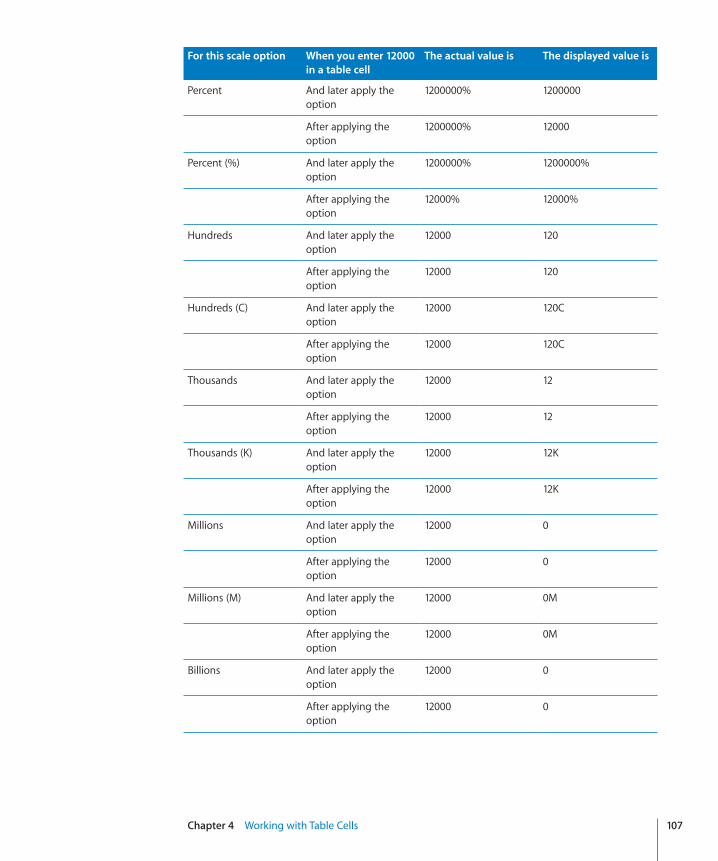
Chapter 4 Working with Table Cells 107
For this scale option When you enter 12000 in a table cell
The actual value is The displayed value is
Percent And later apply the option
1200000% 1200000
After applying the option
1200000% 12000
Percent (%) And later apply the option
1200000% 1200000%
After applying the option
12000% 12000%
Hundreds And later apply the option
12000 120
After applying the option
12000 120
Hundreds (C) And later apply the option
12000 120C
After applying the option
12000 120C
Thousands And later apply the option
12000 12
After applying the option
12000 12
Thousands (K) And later apply the option
12000 12K
After applying the option
12000 12K
Millions And later apply the option
12000 0
After applying the option
12000 0
Millions (M) And later apply the option
12000 0M
After applying the option
12000 0M
Billions And later apply the option
12000 0
After applying the option
12000 0
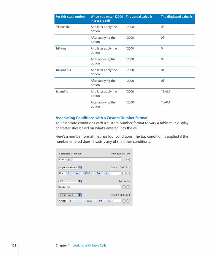
For this scale option When you enter 12000 in a table cell
The actual value is The displayed value is
Billions (B) And later apply the option
12000 0B
After applying the option
12000 0B
Trillions And later apply the option
12000 0
After applying the option
12000 0
Trillions (T) And later apply the option
12000 0T
After applying the option
12000 0T
Scientific And later apply the option
12000 1E+0.4
After applying the option
12000 1E+0.4
Associating Conditions with a Custom Number FormatYou associate conditions with a custom number format to vary a table cell’s display characteristics based on what’s entered into the cell.
Here’s a number format that has four conditions. The top condition is applied if the number entered doesn’t satisfy any of the other conditions.
108 Chapter 4 Working with Table Cells
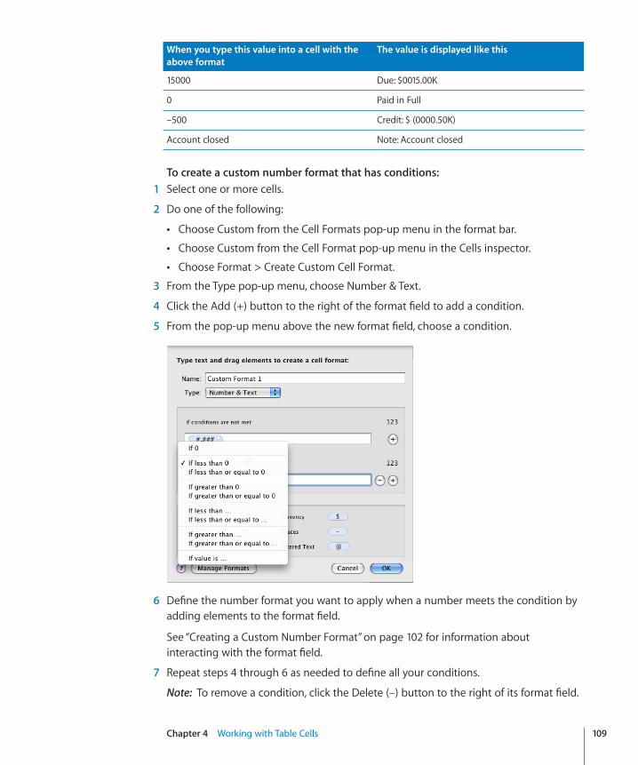
Chapter 4 Working with Table Cells 109
When you type this value into a cell with the above format
The value is displayed like this
15000 Due: $0015.00K
0 Paid in Full
–500 Credit: $ (0000.50K)
Account closed Note: Account closed
To create a custom number format that has conditions:� 1 Select one or more cells.
2 Do one of the following:
Choose Custom from the Cell Formats pop-up menu in the format bar. Â
Choose Custom from the Cell Format pop-up menu in the Cells inspector. Â
Choose Format > Create Custom Cell Format. Â
3 From the Type pop-up menu, choose Number & Text.
4 Click the Add (+) button to the right of the format field to add a condition.
5 From the pop-up menu above the new format field, choose a condition.
6 Define the number format you want to apply when a number meets the condition by adding elements to the format field.
See “Creating a Custom Number Format” on page 102 for information about interacting with the format field.
7 Repeat steps 4 through 6 as needed to define all your conditions.
Note: To remove a condition, click the Delete (–) button to the right of its format field.
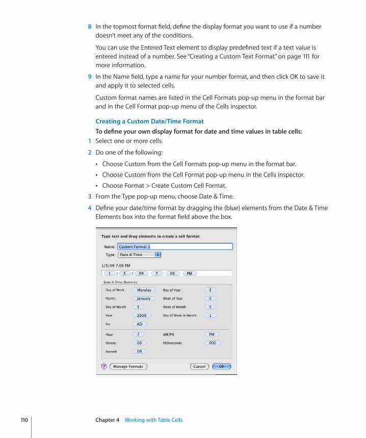
8 In the topmost format field, define the display format you want to use if a number doesn’t meet any of the conditions.
You can use the Entered Text element to display predefined text if a text value is entered instead of a number. See “Creating a Custom Text Format” on page 111 for more information.
9 In the Name field, type a name for your number format, and then click OK to save it and apply it to selected cells.
Custom format names are listed in the Cell Formats pop-up menu in the format bar and in the Cell Format pop-up menu of the Cells inspector.
Creating a Custom Date/Time FormatTo define your own display format for date and time values in table cells:
1 Select one or more cells.
2 Do one of the following:
Choose Custom from the Cell Formats pop-up menu in the format bar. Â
Choose Custom from the Cell Format pop-up menu in the Cells inspector. Â
Choose Format > Create Custom Cell Format. Â
3 From the Type pop-up menu, choose Date & Time.
4 Define your date/time format by dragging the (blue) elements from the Date & Time Elements box into the format field above the box.
110 Chapter 4 Working with Table Cells
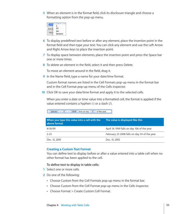
Chapter 4 Working with Table Cells 111
5 When an element is in the format field, click its disclosure triangle and choose a formatting option from the pop-up menu.
6 To display predefined text before or after any element, place the insertion point in the format field and then type your text. You can click any element and use the Left Arrow and Right Arrow keys to place the insertion point.
7 To display space between elements, place the insertion point and press the Space bar one or more times.
8 To delete an element in the field, select it and then press Delete.
To move an element around in the field, drag it.
9 In the Name field, type a name for your date/time format.
Custom format names are listed in the Cell Formats pop-up menu in the format bar and in the Cell Format pop-up menu of the Cells inspector.
10 Click OK to save your date/time format and apply it to the selected cells.
When you enter a date or time value into a formatted cell, the format is applied if the value entered contains a hyphen (-) or a slash (/).
When you type this value into a cell with the above format
The value is displayed like this
4/16/99 April 16 1999 falls on day 106 of the year
2-23 February 23 2008 falls on day 54 of the year
Dec. 15, 2010 Dec. 15, 2010
Creating a Custom Text FormatYou can define text to display before or after a value entered into a table cell when no other format has been applied to the cell.
To define text to display in table cells: 1 Select one or more cells.
2 Do one of the following:
Choose Custom from the Cell Formats pop-up menu in the format bar. Â
Choose Custom from the Cell Format pop-up menu in the Cells inspector. Â
Choose Format > Create Custom Cell Format. Â
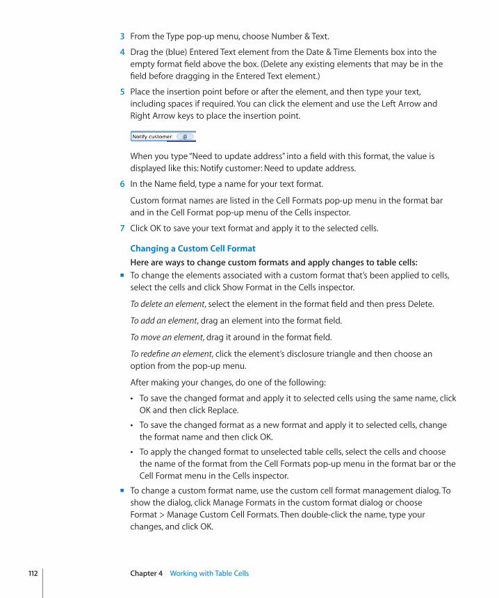
3 From the Type pop-up menu, choose Number & Text.
4 Drag the (blue) Entered Text element from the Date & Time Elements box into the empty format field above the box. (Delete any existing elements that may be in the field before dragging in the Entered Text element.)
5 Place the insertion point before or after the element, and then type your text, including spaces if required. You can click the element and use the Left Arrow and Right Arrow keys to place the insertion point.
When you type “Need to update address” into a field with this format, the value is displayed like this: Notify customer: Need to update address.
6 In the Name field, type a name for your text format.
Custom format names are listed in the Cell Formats pop-up menu in the format bar and in the Cell Format pop-up menu of the Cells inspector.
7 Click OK to save your text format and apply it to the selected cells.
Changing a Custom Cell FormatHere are ways to change custom formats and apply changes to table cells:�To change the elements associated with a custom format that’s been applied to cells, m
select the cells and click Show Format in the Cells inspector.
To delete an element, select the element in the format field and then press Delete.
To add an element, drag an element into the format field.
To move an element, drag it around in the format field.
To redefine an element, click the element’s disclosure triangle and then choose an option from the pop-up menu.
After making your changes, do one of the following:
To save the changed format and apply it to selected cells using the same name, click ÂOK and then click Replace.
To save the changed format as a new format and apply it to selected cells, change Âthe format name and then click OK.
To apply the changed format to unselected table cells, select the cells and choose Âthe name of the format from the Cell Formats pop-up menu in the format bar or the Cell Format menu in the Cells inspector.
To change a custom format name, use the custom cell format management dialog. To m
show the dialog, click Manage Formats in the custom format dialog or choose Format > Manage Custom Cell Formats. Then double-click the name, type your changes, and click OK.
112 Chapter 4 Working with Table Cells
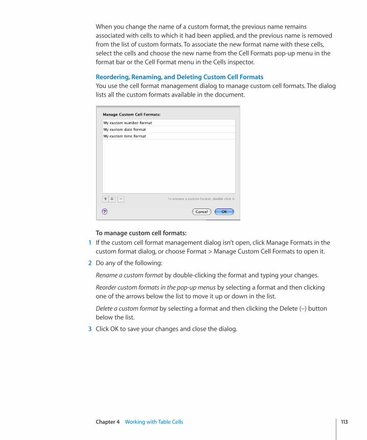
Chapter 4 Working with Table Cells 113
When you change the name of a custom format, the previous name remains associated with cells to which it had been applied, and the previous name is removed from the list of custom formats. To associate the new format name with these cells, select the cells and choose the new name from the Cell Formats pop-up menu in the format bar or the Cell Format menu in the Cells inspector.
Reordering, Renaming, and Deleting Custom Cell FormatsYou use the cell format management dialog to manage custom cell formats. The dialog lists all the custom formats available in the document.
To manage custom cell formats:� 1 If the custom cell format management dialog isn’t open, click Manage Formats in the
custom format dialog, or choose Format > Manage Custom Cell Formats to open it.
2 Do any of the following:
Rename a custom format by double-clicking the format and typing your changes.
Reorder custom formats in the pop-up menus by selecting a format and then clicking one of the arrows below the list to move it up or down in the list.
Delete a custom format by selecting a format and then clicking the Delete (–) button below the list.
3 Click OK to save your changes and close the dialog.
114
This chapter explains how to use table styles to quickly and consistently manage the appearance of tables.
The Numbers templates include a variety of table styles that are ready to use. You can also modify the template styles or create your own styles.
Using Table StylesYou can use different visual characteristics to distinguish different tables in your Numbers spreadsheet. For example, you can format a table containing inputs and assumptions using a blue background and matching borders, and format another table containing calculation results using a gray background and matching borders.
The simplest way to change the appearance of a table is to apply a table style to it. Table styles also ensure that tables are consistently formatted. A table style is predefined formatting that you can apply to a table with the click of a mouse. A table style predefines the following attributes:
The table background (color or image) and its opacity Â
The stroke, color, and opacity of the outside border of body cells, and the outside Âborders of the header row, header column, and footer row
The background (color or image and opacity) and the text attributes of table cells, Âincluding header and footer cells
To learn how to Go to
Format a table using a table style “Applying Table Styles” on page 115
Modify a table’s style “Modifying Table Style Attributes” on page 115
“Copying and Pasting Table Styles” on page 116
Change a table’s default table style “Using the Default Table Style” on page 116
5Working with Table Styles
Chapter 5 Working with Table Styles 115
To learn how to Go to
Save the formatting you apply to a table as a new table style
“Creating New Table Styles” on page 116
Change the name of a table style “Renaming a Table Style” on page 117
Remove a table style from a spreadsheet “Deleting a Table Style” on page 117
Applying Table StylesAfter applying a table style to a table, you can change any of the formatting defined by the style. Such a change is called an override. If you later assign a different style to the table, you can keep or remove any overrides you created.
Here are ways to apply a table style:�To replace a table’s existing style and remove any overrides, click the arrow to the right m
of the style you want to apply and then choose Clear and Apply Style.
You can also choose Format > Reapply Table Style.
To replace a table’s existing style but keep any overrides, select the table and then click m
the name of a style in the Styles pane at the left of the window. You can also select a table, click the arrow to the right of the style you want to apply, and then choose Apply Style.
You can also drag a style name from the Styles pane to a table. The table doesn’t need to be selected in this case.
To replace the style of all tables in a sheet but keep any overrides, drag a style name m
from the Styles pane to a sheet icon in the Sheets pane.
Modifying Table Style AttributesYou can change a table’s appearance by modifying the attributes of the table’s style.
Here are ways to modify table style attributes:�To change the background color of a table, header cells, or body cells, select the table m
or cells and click the Fill well in the format bar.
You can use the Cell Background controls in the Table inspector to make more extensive changes to the selection. “Filling Objects with Colors or Images” on page 225 provides instructions for these controls.
To change the opacity of the background, use the Opacity controls in the Graphic inspector. See “Adjusting Opacity” on page 224 for instructions.
To change the stroke and color of table cell borders, follow the instructions in m
“Formatting Table Cell Borders” on page 87.
To format text in one or more cells, select the cells. m
To modify the color, alignment, and spacing of text within a cell, use the format bar or the Text inspector (click Inspector in the toolbar and click the Text inspector button).
To modify font attributes, use the Fonts window (click Fonts in the toolbar).
If you want to use the changes you make to redefine the table style for the whole spreadsheet, click the arrow to the right of the style and then choose “Redefine Style from Table.” All tables in the spreadsheet that use the style are updated to reflect the changes you made, but overrides are maintained.
You can also create a new style using the changes you’ve made by clicking the arrow to the right of the style and then choosing Create New Style.
Copying and Pasting Table StylesYou can change a table’s appearance by copying and pasting table and table cell styles.
Here are ways to copy and paste table styles:�To copy a cell’s style, select the cell and choose Format > Copy Style. m
To apply a copied cell style to other cells, select the cells and choose m
Format > Paste Style.
To paste a copied table using the spreadsheet’s default table style, choose m
Edit > “Paste and Match Style.”
Using the Default Table StyleEvery spreadsheet has a table style that’s designated as the default table style. It’s the table style that’s applied to new tables.
To change the default table style:�Click the arrow to the right of the style you want to use as the default table style, and m
then choose “Set as Default Style for New Tables.”
To use the default table style for a reusable table you define, follow the instructions in “Defining Reusable Tables” on page 53.
Creating New Table StylesYou can create a new table style by reformatting a table and saving the formatting as a table style.
To create a new table style:� 1 Use the instructions in “Modifying Table Style Attributes” on page 115 to achieve the
visual effects you want.
116 Chapter 5 Working with Table Styles
Chapter 5 Working with Table Styles 117
2 Select the table, click the arrow to the right of any style in the Styles pane, and then choose Create New Style.
3 Type a unique name for your new table style, and click OK.
The new table style now appears in the Styles pane and can be applied to any table in your spreadsheet.
To make a new table style available in other spreadsheets, create a template from the spreadsheet. See “Saving a Spreadsheet as a Template” on page 38 for details.
Renaming a Table StyleYou can change the name of a table style.
To rename a table style:� 1 Click the arrow to the right of the style in the Styles pane.
2 Choose Rename Style.
3 Edit the style name, making sure it’s unique in the spreadsheet.
4 Press Return.
Deleting a Table StyleWhen you delete a table style that’s used in a spreadsheet, you need to choose a different style to replace it.
To delete a style:� 1 Click the arrow to the right of the style in the Styles pane.
2 Choose Delete Style.
3 If the style you want to delete is being used in the current spreadsheet, choose a style to replace it and then click OK.
118
This chapter explains how to perform calculations in table cells by using formulas.
The Elements of FormulasA formula performs a calculation and displays the result in the cell where you place the formula. A cell containing a formula is referred to as a formula cell.
For example, in the bottom cell of a column you can insert a formula that sums the numbers in all the cells above it. If any of the values in the cells above the formula cell change, the sum displayed in the formula cell updates automatically.
A formula performs calculations using specific values you provide. The values can be numbers or text (constants) you type into the formula. Or they can be values that reside in table cells you identify in the formula by using cell references. Formulas use operators and functions to perform calculations using the values you provide:
 Operators are symbols that initiate operations, such as arithmetic and comparison operations. You use the symbols in formulas to indicate the operation you want to use. For example, the symbol + adds values, and the symbol = compares two values to determine whether they’re equal.
=A2 + 16:� A formula that uses an operator to add two values.
=:� Always precedes a formula.
A2:� A cell reference. A2 refers to the second cell in the first column.
+:� An arithmetic operator that adds the value that precedes it with the value that follows it.
16:� A numeric constant.
 Functions are predefined, named operations, such as SUM and AVERAGE. To use a function, you enter its name and, in parentheses following the name, you provide the arguments the function needs. Arguments specify the values the function uses when it performs its operations.
6Using Formulas in Tables
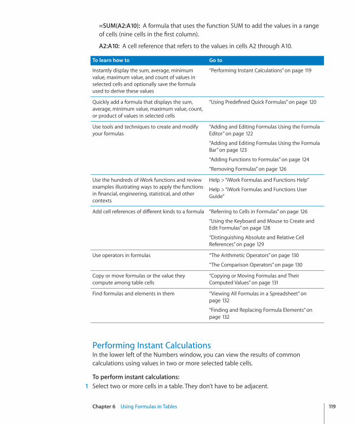
Chapter 6 Using Formulas in Tables 119
=SUM(A2:�A10):� A formula that uses the function SUM to add the values in a range of cells (nine cells in the first column).
A2:�A10:� A cell reference that refers to the values in cells A2 through A10.
To learn how to Go to
Instantly display the sum, average, minimum value, maximum value, and count of values in selected cells and optionally save the formula used to derive these values
“Performing Instant Calculations” on page 119
Quickly add a formula that displays the sum, average, minimum value, maximum value, count, or product of values in selected cells
“Using Predefined Quick Formulas” on page 120
Use tools and techniques to create and modify your formulas
“Adding and Editing Formulas Using the Formula Editor” on page 122
“Adding and Editing Formulas Using the Formula Bar” on page 123
“Adding Functions to Formulas” on page 124
“Removing Formulas” on page 126
Use the hundreds of iWork functions and review examples illustrating ways to apply the functions in financial, engineering, statistical, and other contexts
Help > “iWork Formulas and Functions Help”
Help > “iWork Formulas and Functions User Guide”
Add cell references of different kinds to a formula “Referring to Cells in Formulas” on page 126
“Using the Keyboard and Mouse to Create and Edit Formulas” on page 128
“Distinguishing Absolute and Relative Cell References” on page 129
Use operators in formulas “The Arithmetic Operators” on page 130
“The Comparison Operators” on page 130
Copy or move formulas or the value they compute among table cells
“Copying or Moving Formulas and Their Computed Values” on page 131
Find formulas and elements in them “Viewing All Formulas in a Spreadsheet” on page 132
“Finding and Replacing Formula Elements” on page 132
Performing Instant CalculationsIn the lower left of the Numbers window, you can view the results of common calculations using values in two or more selected table cells.
To perform instant calculations:� 1 Select two or more cells in a table. They don’t have to be adjacent.
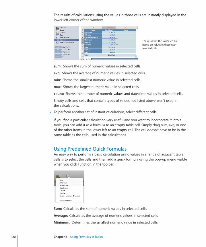
The results of calculations using the values in those cells are instantly displayed in the lower left corner of the window.
The results in the lower left are based on values in these two selected cells.
sum:� Shows the sum of numeric values in selected cells.
avg:� Shows the average of numeric values in selected cells.
min:� Shows the smallest numeric value in selected cells.
max:� Shows the largest numeric value in selected cells.
count:� Shows the number of numeric values and date/time values in selected cells.
Empty cells and cells that contain types of values not listed above aren’t used in the calculations.
2 To perform another set of instant calculations, select different cells.
If you find a particular calculation very useful and you want to incorporate it into a table, you can add it as a formula to an empty table cell. Simply drag sum, avg, or one of the other items in the lower left to an empty cell. The cell doesn’t have to be in the same table as the cells used in the calculations.
Using Predefined Quick FormulasAn easy way to perform a basic calculation using values in a range of adjacent table cells is to select the cells and then add a quick formula using the pop-up menu visible when you click Function in the toolbar.
Sum:� Calculates the sum of numeric values in selected cells.
Average:� Calculates the average of numeric values in selected cells.
Minimum:� Determines the smallest numeric value in selected cells.
120 Chapter 6 Using Formulas in Tables
Chapter 6 Using Formulas in Tables 121
Maximum:� Determines the largest numeric value in selected cells
Count:� Determines the number of numeric values and date/time values in selected cells.
Product:� Multiplies all the numeric values in selected cells.
You can also choose Insert > Function and use the submenu that appears.
Empty cells and cells containing types of values not listed are ignored.
Here are ways to add a quick formula:�To use selected values in a column or a row, select the cells, click Function in the m
toolbar, and then choose a calculation from the pop-up menu.
If the cells are in the same column, Numbers places the formula in the first empty cell beneath the selected cells. If there is no empty cell, Numbers adds a row to hold the formula.
If the cells are in the same row, Numbers places the formula in the first empty cell to the right of the selected cells. If there is no empty cell, Numbers adds a column to hold the formula.
To use m all the values in a column’s body cells, click the column’s header cell or reference tab, click Function in the toolbar, and then choose a calculation from the pop-up menu.
Numbers places the formula in a footer row. If a footer row doesn’t exist, Numbers adds one.
To use m all the values in a row, click the row’s header cell or reference tab, click Function in the toolbar, and then choose a calculation from the pop-up menu.
Numbers places the formula in a new column.
Creating Your Own FormulasAlthough you can use several shortcut techniques to add formulas that perform simple calculations (see “Performing Instant Calculations” on page 119 and “Using Predefined Quick Formulas” on page 120), when you want more control you use the formula tools to add formulas.
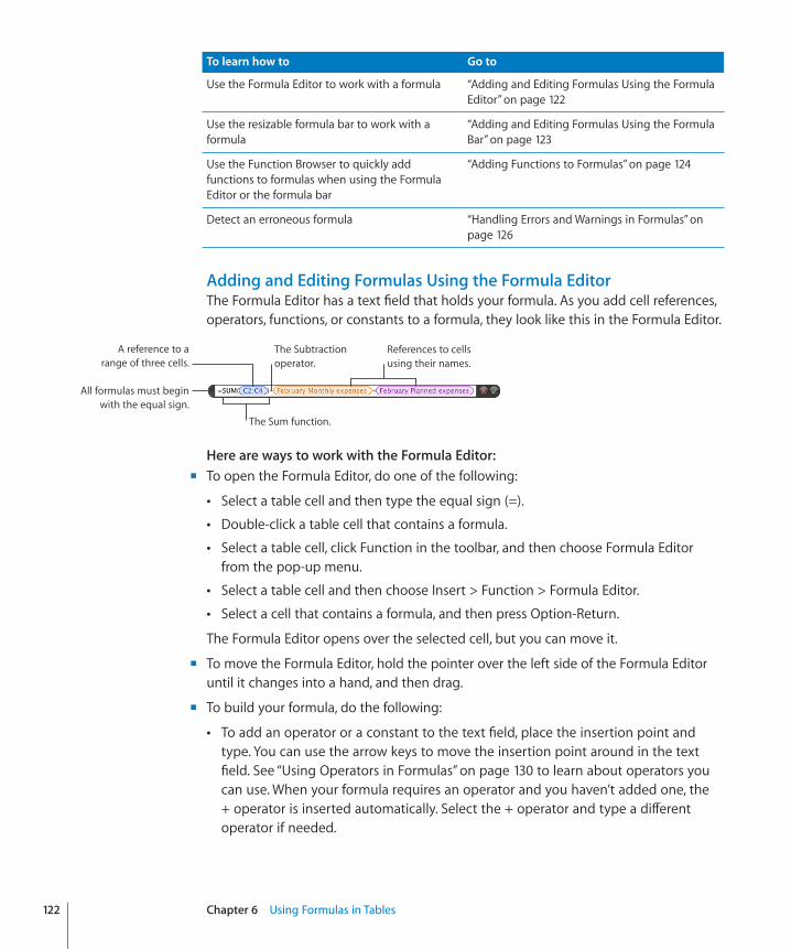
To learn how to Go to
Use the Formula Editor to work with a formula “Adding and Editing Formulas Using the Formula Editor” on page 122
Use the resizable formula bar to work with a formula
“Adding and Editing Formulas Using the Formula Bar” on page 123
Use the Function Browser to quickly add functions to formulas when using the Formula Editor or the formula bar
“Adding Functions to Formulas” on page 124
Detect an erroneous formula “Handling Errors and Warnings in Formulas” on page 126
Adding and Editing Formulas Using the Formula EditorThe Formula Editor has a text field that holds your formula. As you add cell references, operators, functions, or constants to a formula, they look like this in the Formula Editor.
All formulas must begin with the equal sign.
The Sum function.
References to cells using their names.
A reference to a range of three cells.
The Subtraction operator.
Here are ways to work with the Formula Editor:�To open the Formula Editor, do one of the following: m
Select a table cell and then type the equal sign (=). Â
Double-click a table cell that contains a formula. Â
Select a table cell, click Function in the toolbar, and then choose Formula Editor Âfrom the pop-up menu.
Select a table cell and then choose Insert > Function > Formula Editor. Â
Select a cell that contains a formula, and then press Option-Return. Â
The Formula Editor opens over the selected cell, but you can move it.
To move the Formula Editor, hold the pointer over the left side of the Formula Editor m
until it changes into a hand, and then drag.
To build your formula, do the following: m
To add an operator or a constant to the text field, place the insertion point and Âtype. You can use the arrow keys to move the insertion point around in the text field. See “Using Operators in Formulas” on page 130 to learn about operators you can use. When your formula requires an operator and you haven’t added one, the + operator is inserted automatically. Select the + operator and type a different operator if needed.
122 Chapter 6 Using Formulas in Tables
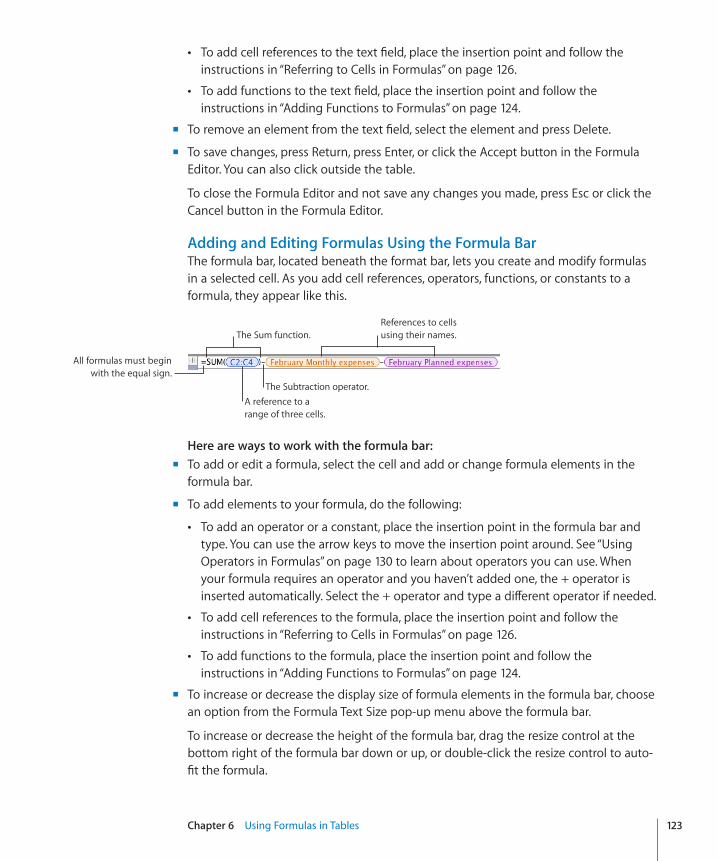
Chapter 6 Using Formulas in Tables 123
To add cell references to the text field, place the insertion point and follow the Âinstructions in “Referring to Cells in Formulas” on page 126.
To add functions to the text field, place the insertion point and follow the Âinstructions in “Adding Functions to Formulas” on page 124.
To remove an element from the text field, select the element and press Delete. m
To save changes, press Return, press Enter, or click the Accept button in the Formula m
Editor. You can also click outside the table.
To close the Formula Editor and not save any changes you made, press Esc or click the Cancel button in the Formula Editor.
Adding and Editing Formulas Using the Formula BarThe formula bar, located beneath the format bar, lets you create and modify formulas in a selected cell. As you add cell references, operators, functions, or constants to a formula, they appear like this.
The Subtraction operator.
References to cells using their names.The Sum function.
All formulas must begin with the equal sign.
A reference to a range of three cells.
Here are ways to work with the formula bar:�To add or edit a formula, select the cell and add or change formula elements in the m
formula bar.
To add elements to your formula, do the following: m
To add an operator or a constant, place the insertion point in the formula bar and Âtype. You can use the arrow keys to move the insertion point around. See “Using Operators in Formulas” on page 130 to learn about operators you can use. When your formula requires an operator and you haven’t added one, the + operator is inserted automatically. Select the + operator and type a different operator if needed.
To add cell references to the formula, place the insertion point and follow the Âinstructions in “Referring to Cells in Formulas” on page 126.
To add functions to the formula, place the insertion point and follow the Âinstructions in “Adding Functions to Formulas” on page 124.
To increase or decrease the display size of formula elements in the formula bar, choose m
an option from the Formula Text Size pop-up menu above the formula bar.
To increase or decrease the height of the formula bar, drag the resize control at the bottom right of the formula bar down or up, or double-click the resize control to auto-fit the formula.
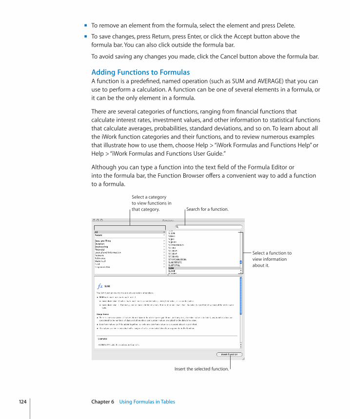
To remove an element from the formula, select the element and press Delete. m
To save changes, press Return, press Enter, or click the Accept button above the m
formula bar. You can also click outside the formula bar.
To avoid saving any changes you made, click the Cancel button above the formula bar.
Adding Functions to FormulasA function is a predefined, named operation (such as SUM and AVERAGE) that you can use to perform a calculation. A function can be one of several elements in a formula, or it can be the only element in a formula.
There are several categories of functions, ranging from financial functions that calculate interest rates, investment values, and other information to statistical functions that calculate averages, probabilities, standard deviations, and so on. To learn about all the iWork function categories and their functions, and to review numerous examples that illustrate how to use them, choose Help > “iWork Formulas and Functions Help” or Help > “iWork Formulas and Functions User Guide.”
Although you can type a function into the text field of the Formula Editor or into the formula bar, the Function Browser offers a convenient way to add a function to a formula.
Select a function to view information about it.
Search for a function.
Insert the selected function.
Select a category to view functions in that category.
124 Chapter 6 Using Formulas in Tables
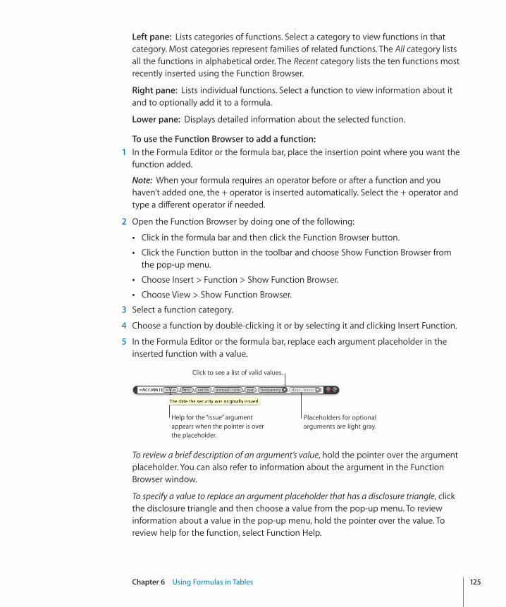
Chapter 6 Using Formulas in Tables 125
Left pane:� Lists categories of functions. Select a category to view functions in that category. Most categories represent families of related functions. The All category lists all the functions in alphabetical order. The Recent category lists the ten functions most recently inserted using the Function Browser.
Right pane:� Lists individual functions. Select a function to view information about it and to optionally add it to a formula.
Lower pane:� Displays detailed information about the selected function.
To use the Function Browser to add a function:� 1 In the Formula Editor or the formula bar, place the insertion point where you want the
function added.
Note: When your formula requires an operator before or after a function and you haven’t added one, the + operator is inserted automatically. Select the + operator and type a different operator if needed.
2 Open the Function Browser by doing one of the following:
Click in the formula bar and then click the Function Browser button. Â
Click the Function button in the toolbar and choose Show Function Browser from Âthe pop-up menu.
Choose Insert > Function > Show Function Browser. Â
Choose View > Show Function Browser. Â
3 Select a function category.
4 Choose a function by double-clicking it or by selecting it and clicking Insert Function.
5 In the Formula Editor or the formula bar, replace each argument placeholder in the inserted function with a value.
Help for the “issue” argument appears when the pointer is over the placeholder.
Placeholders for optional arguments are light gray.
Click to see a list of valid values.
To review a brief description of an argument’s value, hold the pointer over the argument placeholder. You can also refer to information about the argument in the Function Browser window.
To specify a value to replace an argument placeholder that has a disclosure triangle, click the disclosure triangle and then choose a value from the pop-up menu. To review information about a value in the pop-up menu, hold the pointer over the value. To review help for the function, select Function Help.
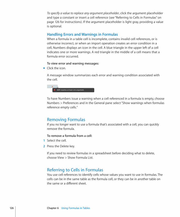
To specify a value to replace any argument placeholder, click the argument placeholder and type a constant or insert a cell reference (see “Referring to Cells in Formulas” on page 126 for instructions). If the argument placeholder is light gray, providing a value is optional.
Handling Errors and Warnings in FormulasWhen a formula in a table cell is incomplete, contains invalid cell references, or is otherwise incorrect, or when an import operation creates an error condition in a cell, Numbers displays an icon in the cell. A blue triangle in the upper left of a cell indicates one or more warnings. A red triangle in the middle of a cell means that a formula error occurred.
To view error and warning messages:�Click the icon. m
A message window summarizes each error and warning condition associated with the cell.
To have Numbers issue a warning when a cell referenced in a formula is empty, choose Numbers > Preferences and in the General pane select “Show warnings when formulas reference empty cells.”
Removing FormulasIf you no longer want to use a formula that’s associated with a cell, you can quickly remove the formula.
To remove a formula from a cell:� 1 Select the cell.
2 Press the Delete key.
If you need to review formulas in a spreadsheet before deciding what to delete, choose View > Show Formula List.
Referring to Cells in FormulasYou use cell references to identify cells whose values you want to use in formulas. The cells can be in the same table as the formula cell, or they can be in another table on the same or a different sheet.
126 Chapter 6 Using Formulas in Tables
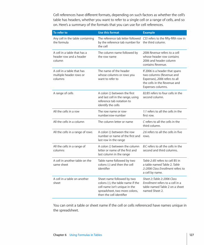
Chapter 6 Using Formulas in Tables 127
Cell references have different formats, depending on such factors as whether the cell’s table has headers, whether you want to refer to a single cell or a range of cells, and so on. Here’s a summary of the formats that you can use for cell references.
To refer to Use this format Example
Any cell in the table containing the formula
The reference tab letter followed by the reference tab number for the cell
C55 refers to the fifty-fifth row in the third column.
A cell in a table that has a header row and a header column
The column name followed by the row name
2006 Revenue refers to a cell whose header row contains 2006 and header column contains Revenue.
A cell in a table that has multiple header rows or columns
The name of the header whose columns or rows you want to refer to
If 2006 is a header that spans two columns (Revenue and Expenses), 2006 refers to all the cells in the Revenue and Expenses columns.
A range of cells A colon (:) between the first and last cell in the range, using reference tab notation to identify the cells
B2:B5 refers to four cells in the second column.
All the cells in a row The row name or row-number:row-number
1:1 refers to all the cells in the first row.
All the cells in a column The column letter or name C refers to all the cells in the third column.
All the cells in a range of rows A colon (:) between the row number or name of the first and last row in the range
2:6 refers to all the cells in five rows.
All the cells in a range of columns
A colon (:) between the column letter or name of the first and last column in the range
B:C refers to all the cells in the second and third columns.
A cell in another table on the same sheet
Table name followed by two colons (::) and then the cell identifier
Table 2::B5 refers to cell B5 in a table named Table 2. Table 2::2006 Class Enrollment refers to a cell by name.
A cell in a table on another sheet
Sheet name followed by two colons (::), the table name if the cell name isn’t unique in the spreadsheet, two more colons, then the cell identifier
Sheet 2::Table 2::2006 Class Enrollment refers to a cell in a table named Table 2 on a sheet named Sheet 2.
You can omit a table or sheet name if the cell or cells referenced have names unique in the spreadsheet.
When you reference a cell in a multi-row or multi-column header, you’ll notice the following behavior:
The name in the header cell closest to the cell referring to it is used. For example, if Âa table has two header rows, and B1 contains “Dog” and B2 contains “Cat,” when you save a formula that uses “Dog,” “Cat” is saved instead.
However, if “Cat” appears in another header cell in the spreadsheet, “Dog” is retained. Â
To learn how to insert cell references into a formula, see “Using the Keyboard and Mouse to Create and Edit Formulas” on page 128. See “Distinguishing Absolute and Relative Cell References” on page 129 to learn about absolute and relative forms of cell references, which are important when you need to copy or move a formula.
Using the Keyboard and Mouse to Create and Edit FormulasYou can type cell references into a formula, or you can insert cell references using mouse or keyboard shortcuts.
Here are ways to insert cell references:�To use a keyboard shortcut to enter a cell reference, place the insertion point in the m
Formula Editor or formula bar and do one of the following:
To refer to a single cell, press Option and then use the arrow keys to select the cell. Â
To refer to a range of cells, press and hold Shift-Option after selecting the first cell in Âthe range until the last cell in the range is selected.
To refer to cells in another table on the same or a different sheet, select the table Âby pressing Option-Command–Page Down to move downward through tables or Option-Command–Page Up to move upward through tables. Then use one of the two techniques above to select one or more cells in the table.
To specify absolute and relative attributes of a cell reference after inserting one, Âclick the inserted reference and press Command-K to cycle through the options. See “Distinguishing Absolute and Relative Cell References” on page 129 for more information.
To use the mouse to enter a cell reference, place the insertion point in the Formula m
Editor or formula bar and do one of the following in the same table as the formula cell or in a different table on the same or a different sheet:
To refer to a single cell, click the cell. Â
To refer to all the cells in a column or a row, click the reference tab for the column Âor row.
To refer to a range of cells, click a cell in the range and drag up, down, left, or right Âto select or resize the cell range.
128 Chapter 6 Using Formulas in Tables
Chapter 6 Using Formulas in Tables 129
To specify absolute and relative attributes of a cell reference after inserting one, Âclick the inserted reference, click its disclosure triangle, and choose an option from the pop-up menu. See “Distinguishing Absolute and Relative Cell References” on page 129 for more information.
The cell reference inserted uses names instead of reference tab notations if “Use header cell names as references” is selected in the General pane of Numbers preferences.
To type a cell reference, place the insertion point in the Formula Editor or formula bar, m
and enter the cell reference using one of the formats listed in “Referring to Cells in Formulas” on page 126.
When you type a cell reference that includes the name of a header cell, table, or sheet, after typing three characters a list of suggestions pops up if the characters you typed match one or more names in your spreadsheet. You can select from the list or continue typing. To disable name suggestions, choose Numbers > Preferences and deselect “Use header cell names as references” in the General pane.
Distinguishing Absolute and Relative Cell ReferencesUse absolute and relative forms of a cell reference to indicate the cell to which you want the reference to point if you copy or move its formula.
If a cell reference is relative (A1), when its formula moves, it stays the same. However, when the formula is cut or copied and then pasted, the cell reference changes so that it retains the same position relative to the formula cell. For example, if a formula containing A1 appears in C4 and you copy the formula and paste it in C5, the cell reference in C5 becomes A2.
If the row and column components of a cell reference are absolute ($A$1), when its formula is moved or copied and pasted, the cell reference doesn’t change. You use the dollar sign ($) to designate as absolute a row or column component. For example, if a formula containing $A$1 appears in C4 and you copy the formula and paste it in C5 or to D5, the cell reference in C5 or D5 remains $A$1.
If the row component of a cell reference is absolute (A$1), the column component is relative and may change to retain its position relative to the formula cell. For example, if a formula containing A$1 appears in C4 and you copy the formula and paste it in D5, the cell reference in D5 becomes B$1.
If the column component of a cell reference is absolute ($A1), the row component is relative and may change to retain its position relative to the formula cell. For example, if a formula containing $A1 appears in C4 and you copy the formula and paste it in C5 or D5, the cell reference in C5 and D5 becomes $A2.
If both the formula cell and its referenced cells are selected, when you move the selection, the formula stays the same, regardless of the relative or absolute settings of the cell references.
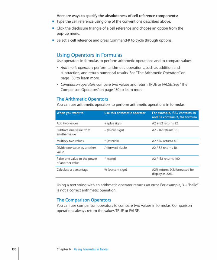
Here are ways to specify the absoluteness of cell reference components:�Type the cell reference using one of the conventions described above. m
Click the disclosure triangle of a cell reference and choose an option from the m
pop-up menu.
Select a cell reference and press Command-K to cycle through options. m
Using Operators in FormulasUse operators in formulas to perform arithmetic operations and to compare values:
 Arithmetic operators perform arithmetic operations, such as addition and subtraction, and return numerical results. See “The Arithmetic Operators” on page 130 to learn more.
 Comparison operators compare two values and return TRUE or FALSE. See “The Comparison Operators” on page 130 to learn more.
The Arithmetic OperatorsYou can use arithmetic operators to perform arithmetic operations in formulas.
When you want to Use this arithmetic operator For example, if A2 contains 20 and B2 contains 2, the formula
Add two values + (plus sign) A2 + B2 returns 22.
Subtract one value from another value
– (minus sign) A2 – B2 returns 18.
Multiply two values * (asterisk) A2 * B2 returns 40.
Divide one value by another value
/ (forward slash) A2 / B2 returns 10.
Raise one value to the power of another value
^ (caret) A2 ^ B2 returns 400.
Calculate a percentage % (percent sign) A2% returns 0.2, formatted for display as 20%.
Using a text string with an arithmetic operator returns an error. For example, 3 + “hello” is not a correct arithmetic operation.
The Comparison OperatorsYou can use comparison operators to compare two values in formulas. Comparison operations always return the values TRUE or FALSE.
130 Chapter 6 Using Formulas in Tables
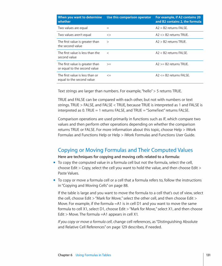
Chapter 6 Using Formulas in Tables 131
When you want to determine whether
Use this comparison operator For example, if A2 contains 20 and B2 contains 2, the formula
Two values are equal = A2 = B2 returns FALSE.
Two values aren’t equal <> A2 <> B2 returns TRUE.
The first value is greater than the second value
> A2 > B2 returns TRUE.
The first value is less than the second value
< A2 < B2 returns FALSE.
The first value is greater than or equal to the second value
>= A2 >= B2 returns TRUE.
The first value is less than or equal to the second value
<= A2 <= B2 returns FALSE.
Text strings are larger than numbers. For example, “hello” > 5 returns TRUE.
TRUE and FALSE can be compared with each other, but not with numbers or text strings. TRUE > FALSE, and FALSE < TRUE, because TRUE is interpreted as 1 and FALSE is interpreted as 0. TRUE = 1 returns FALSE, and TRUE = “SomeText” returns FALSE.
Comparison operations are used primarily in functions such as IF, which compare two values and then perform other operations depending on whether the comparison returns TRUE or FALSE. For more information about this topic, choose Help > iWork Formulas and Functions Help or Help > iWork Formulas and Functions User Guide.
Copying or Moving Formulas and Their Computed ValuesHere are techniques for copying and moving cells related to a formula:� To copy the computed value in a formula cell but not the formula, select the cell, m
choose Edit > Copy, select the cell you want to hold the value, and then choose Edit > Paste Values.
To copy or move a formula cell or a cell that a formula refers to, follow the instructions m
in “Copying and Moving Cells” on page 88.
If the table is large and you want to move the formula to a cell that’s out of view, select the cell, choose Edit > “Mark for Move,” select the other cell, and then choose Edit > Move. For example, if the formula =A1 is in cell D1 and you want to move the same formula to cell X1, select D1, choose Edit > “Mark for Move,” select X1, and then choose Edit > Move. The formula =A1 appears in cell X1.
If you copy or move a formula cell, change cell references, as “Distinguishing Absolute and Relative Cell References” on page 129 describes, if needed.
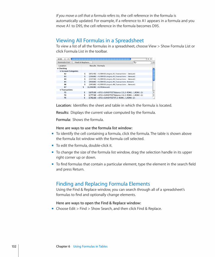
If you move a cell that a formula refers to, the cell reference in the formula is automatically updated. For example, if a reference to A1 appears in a formula and you move A1 to D95, the cell reference in the formula becomes D95.
Viewing All Formulas in a SpreadsheetTo view a list of all the formulas in a spreadsheet, choose View > Show Formula List or click Formula List in the toolbar.
Location:� Identifies the sheet and table in which the formula is located.
Results:� Displays the current value computed by the formula.
Formula:� Shows the formula.
Here are ways to use the formula list window:�To identify the cell containing a formula, click the formula. The table is shown above m
the formula list window with the formula cell selected.
To edit the formula, double-click it. m
To change the size of the formula list window, drag the selection handle in its upper m
right corner up or down.
To find formulas that contain a particular element, type the element in the search field m
and press Return.
Finding and Replacing Formula ElementsUsing the Find & Replace window, you can search through all of a spreadsheet’s formulas to find and optionally change elements.
Here are ways to open the Find & Replace window:�Choose Edit > Find > Show Search, and then click Find & Replace. m
132 Chapter 6 Using Formulas in Tables
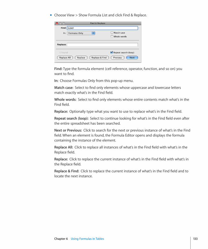
Chapter 6 Using Formulas in Tables 133
Choose View > Show Formula List and click Find & Replace. m
Find:� Type the formula element (cell reference, operator, function, and so on) you want to find.
In:� Choose Formulas Only from this pop-up menu.
Match case:� Select to find only elements whose uppercase and lowercase letters match exactly what’s in the Find field.
Whole words:� Select to find only elements whose entire contents match what’s in the Find field.
Replace:� Optionally type what you want to use to replace what’s in the Find field.
Repeat search (loop):� Select to continue looking for what’s in the Find field even after the entire spreadsheet has been searched.
Next or Previous:� Click to search for the next or previous instance of what’s in the Find field. When an element is found, the Formula Editor opens and displays the formula containing the instance of the element.
Replace All:� Click to replace all instances of what’s in the Find field with what’s in the Replace field.
Replace:� Click to replace the current instance of what’s in the Find field with what’s in the Replace field.
Replace & Find:� Click to replace the current instance of what’s in the Find field and to locate the next instance.

134
This chapter describes how to create and format attractive charts from the data in your tables.
Numbers provides tools for creating your own visually appealing charts to present some or all of the data in one or more tables. By default, the appearance of charts is coordinated with the theme you’re using, but you can adjust colors, textures, shadows, labels, and more to create the look you want or to emphasize various chart elements.
About ChartsUse a chart when you want to visually represent trends or relationships that may be more difficult to see when data is presented in a table. In Numbers you can choose from a variety of 2D or 3D chart types to present your data, including pie charts, line charts, bar charts, column charts, and area charts, depending on which works best to make the point with your data, or use a mixed chart to overlay two chart types within the same figure. You can also graph your data in a two-dimensional scatter chart, using linear or logarithmic scales.
Numbers includes the following types of charts:
Kind of chart Icon
Column
Stacked column
Bar
7Creating Charts from Data
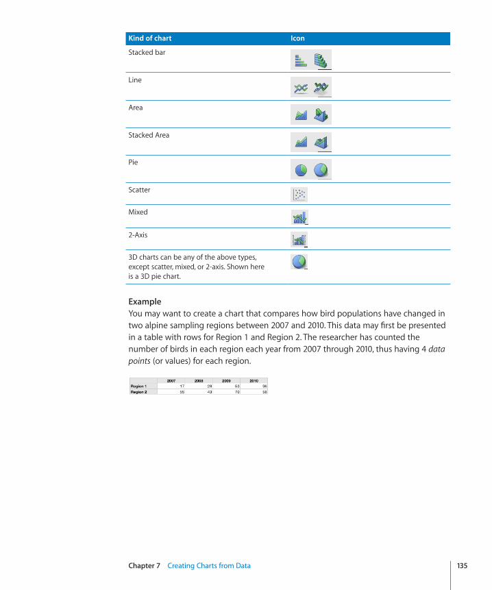
Chapter 7 Creating Charts from Data 135
Kind of chart Icon
Stacked bar
Line
Area
Stacked Area
Pie
Scatter
Mixed
2-Axis
3D charts can be any of the above types, except scatter, mixed, or 2-axis. Shown here is a 3D pie chart.
ExampleYou may want to create a chart that compares how bird populations have changed in two alpine sampling regions between 2007 and 2010. This data may first be presented in a table with rows for Region 1 and Region 2. The researcher has counted the number of birds in each region each year from 2007 through 2010, thus having 4 data points (or values) for each region.
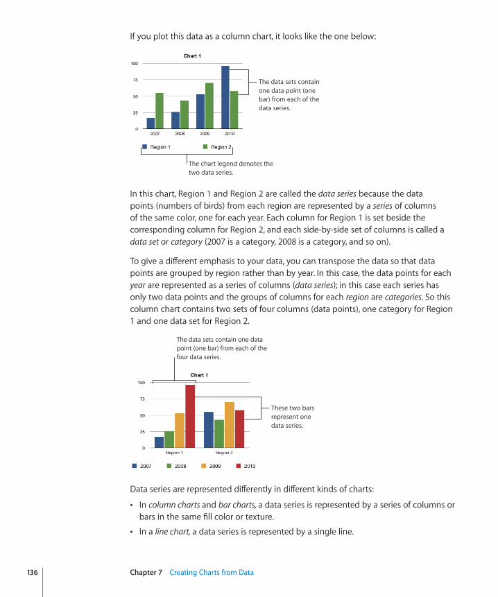
If you plot this data as a column chart, it looks like the one below:
The data sets contain one data point (one bar) from each of the data series.
The chart legend denotes the two data series.
In this chart, Region 1 and Region 2 are called the data series because the data points (numbers of birds) from each region are represented by a series of columns of the same color, one for each year. Each column for Region 1 is set beside the corresponding column for Region 2, and each side-by-side set of columns is called a data set or category (2007 is a category, 2008 is a category, and so on).
To give a different emphasis to your data, you can transpose the data so that data points are grouped by region rather than by year. In this case, the data points for each year are represented as a series of columns (data series); in this case each series has only two data points and the groups of columns for each region are categories. So this column chart contains two sets of four columns (data points), one category for Region 1 and one data set for Region 2.
The data sets contain one data point (one bar) from each of the four data series.
These two bars represent one data series.
Data series are represented differently in different kinds of charts:
In  column charts and bar charts, a data series is represented by a series of columns or bars in the same fill color or texture.
In a  line chart, a data series is represented by a single line.
136 Chapter 7 Creating Charts from Data
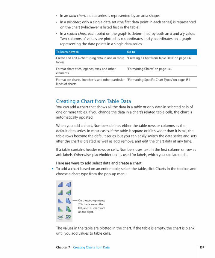
Chapter 7 Creating Charts from Data 137
In an  area chart, a data series is represented by an area shape.
In a  pie chart, only a single data set (the first data point in each series) is represented on the chart (whichever is listed first in the table).
In a  scatter chart, each point on the graph is determined by both an x and a y value. Two columns of values are plotted as x coordinates and y coordinates on a graph representing the data points in a single data series.
To learn how to Go to
Create and edit a chart using data in one or more tables
“Creating a Chart from Table Data” on page 137
Format chart titles, legends, axes, and other elements
“Formatting Charts” on page 143
Format pie charts, line charts, and other particular kinds of charts
“Formatting Specific Chart Types” on page 154
Creating a Chart from Table DataYou can add a chart that shows all the data in a table or only data in selected cells of one or more tables. If you change the data in a chart’s related table cells, the chart is automatically updated.
When you add a chart, Numbers defines either the table rows or columns as the default data series. In most cases, if the table is square or if it’s wider than it is tall, the table rows become the default series, but you can easily switch the data series and sets after the chart is created, as well as add, remove, and edit the chart data at any time.
If a table contains header rows or cells, Numbers uses text in the first column or row as axis labels. Otherwise, placeholder text is used for labels, which you can later edit.
Here are ways to add select data and create a chart:�To add a chart based on an entire table, select the table, click Charts in the toolbar, and m
choose a chart type from the pop-up menu.
On the pop-up menu, 2D charts are on the left, and 3D charts are on the right.
The values in the table are plotted in the chart. If the table is empty, the chart is blank until you add values to table cells.
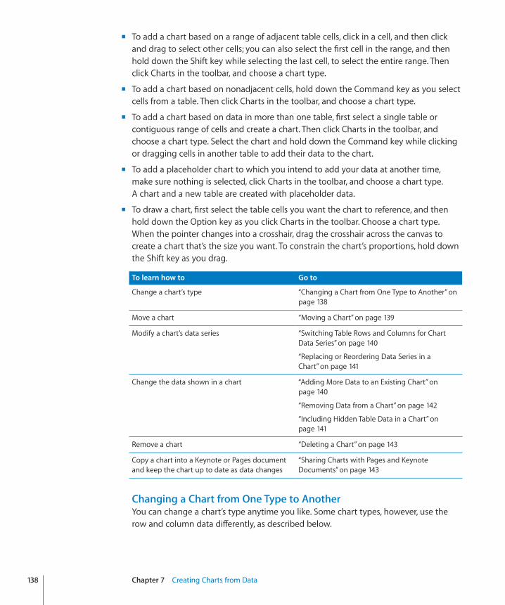
To add a chart based on a range of adjacent table cells, click in a cell, and then click m
and drag to select other cells; you can also select the first cell in the range, and then hold down the Shift key while selecting the last cell, to select the entire range. Then click Charts in the toolbar, and choose a chart type.
To add a chart based on nonadjacent cells, hold down the Command key as you select m
cells from a table. Then click Charts in the toolbar, and choose a chart type.
To add a chart based on data in more than one table, first select a single table or m
contiguous range of cells and create a chart. Then click Charts in the toolbar, and choose a chart type. Select the chart and hold down the Command key while clicking or dragging cells in another table to add their data to the chart.
To add a placeholder chart to which you intend to add your data at another time, m
make sure nothing is selected, click Charts in the toolbar, and choose a chart type. A chart and a new table are created with placeholder data.
To draw a chart, first select the table cells you want the chart to reference, and then m
hold down the Option key as you click Charts in the toolbar. Choose a chart type. When the pointer changes into a crosshair, drag the crosshair across the canvas to create a chart that’s the size you want. To constrain the chart’s proportions, hold down the Shift key as you drag.
To learn how to Go to
Change a chart’s type “Changing a Chart from One Type to Another” on page 138
Move a chart “Moving a Chart” on page 139
Modify a chart’s data series “Switching Table Rows and Columns for Chart Data Series” on page 140
“Replacing or Reordering Data Series in a Chart” on page 141
Change the data shown in a chart “Adding More Data to an Existing Chart” on page 140
“Removing Data from a Chart” on page 142
“Including Hidden Table Data in a Chart” on page 141
Remove a chart “Deleting a Chart” on page 143
Copy a chart into a Keynote or Pages document and keep the chart up to date as data changes
“Sharing Charts with Pages and Keynote Documents” on page 143
Changing a Chart from One Type to AnotherYou can change a chart’s type anytime you like. Some chart types, however, use the row and column data differently, as described below.
138 Chapter 7 Creating Charts from Data
Chapter 7 Creating Charts from Data 139
To change a chart from one type to another:� 1 Select the chart.
2 Do one of the following:
From the pop-up menu at the left end of the format bar, choose a chart type. Â
Control-click the chart, choose Chart Type from the pop-up menu, and select a chart Âtype from the submenu.
Click Inspector in the toolbar, click the Chart inspector button, and then choose a Âchart type from the pop-up menu that appears when you click the chart icon in the upper left.
If you switch to a pie chart, the first data point in each series is represented as a wedge.
If you switch to a scatter chart, each point in the chart requires two values. If the chart is based on an odd number of rows or columns, the last row or column isn’t plotted.
If you switch to a bar, column, area, or line chart, each series in the new chart corresponds to a row or column.
If you switch to a 3D version of a chart, the Chart inspector provides controls for managing object depth, lighting style, and more.
Formatting you’ve applied to the chart you’re changing may not be applied to the new chart. For example, the color fill attribute of data point elements (bars, wedges, and so on) has a different default value for each type of chart. If you’ve changed a column fill color and then change the chart to be a bar chart, the fill color change isn’t retained. Depending on the type of chart, the attributes that may revert to the default styling are value labels and position, text style, series stroke, series shadow, series fill, data point symbols, and data point fills.
When you change a chart’s type and the new type has some of the same attributes, those attributes don’t change. Shared attributes include axes, gridlines, tick marks, axis labels, show minimum value, number format, borders, rotation, shadows, and 3D lighting style. See “Formatting Charts” on page 143 and “Formatting Specific Chart Types” on page 154 for more information.
Bar or column charts, and stacked bar or column charts, share attributes except for value label position. Also, bar and column charts have separate fills.
3D chart shadows are shared across chart types.
Moving a ChartWhen you move a chart to a new location within the same Numbers document, connections to the table cells it references are maintained.
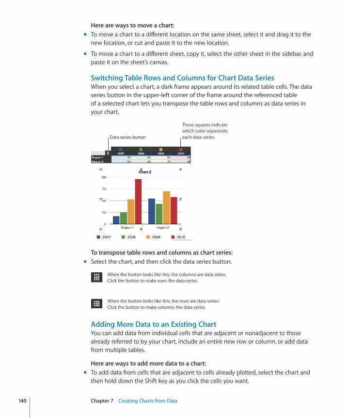
Here are ways to move a chart:�To move a chart to a different location on the same sheet, select it and drag it to the m
new location, or cut and paste it to the new location.
To move a chart to a different sheet, copy it, select the other sheet in the sidebar, and m
paste it on the sheet’s canvas.
Switching Table Rows and Columns for Chart Data SeriesWhen you select a chart, a dark frame appears around its related table cells. The data series button in the upper-left corner of the frame around the referenced table of a selected chart lets you transpose the table rows and columns as data series in your chart.
These squares indicate which color represents each data series.Data series button
To transpose table rows and columns as chart series:�Select the chart, and then click the data series button. m
When the button looks like this, the columns are data series. Click the button to make rows the data series.
When the button looks like this, the rows are data series. Click the button to make columns the data series.
Adding More Data to an Existing ChartYou can add data from individual cells that are adjacent or nonadjacent to those already referred to by your chart, include an entire new row or column, or add data from multiple tables.
Here are ways to add more data to a chart:�To add data from cells that are adjacent to cells already plotted, select the chart and m
then hold down the Shift key as you click the cells you want.
140 Chapter 7 Creating Charts from Data
Chapter 7 Creating Charts from Data 141
To add data from cells that aren’t adjacent to cells already plotted, select the chart and m
then hold down the Command key as you click or drag the cells you want.
To extend the range of adjacent cells whose values are plotted, select the chart. In the m
table, drag the circular control in the lower right of the range to the right or down.
If the chart is a scatter chart, dragging lets you add only an even number of rows or columns.
To add a new row or column of data, select the table and insert the row or column m
between cells that are already plotted. When you add data to the new cells, the data will be plotted in the chart.
To add data from cells in a different table, select the cells with data you want to add, m
and then drag them to the chart.
The new data is added as a new data series. To view or change the chart’s source data, click a data series in the chart to see its table and cells of origin.
To include data from hidden rows and columns in your chart, see “Including Hidden Table Data in a Chart” on page 141.
Including Hidden Table Data in a ChartIf you’ve hidden rows or columns in a table, but want to include or exclude them from a chart, you can elect to do so in the Chart pane of the Chart inspector.
To include or exclude hidden data:� 1 Select the chart, and then click the Inspector button in the toolbar.
2 Click the Chart button in the Inspector window, click Chart, and then do one of the following:
To include hidden data in your chart, select Show Hidden Data. Â
To exclude hidden data from your chart, deselect Show Hidden Data. Â
Replacing or Reordering Data Series in a ChartWhen you add, remove, or reorder data in a chart, your changes don’t affect the table or tables whose data is shown in the chart.
For example, if you want to replace a series of data values in an existing chart with a different data series, you can easily replace any referenced row or column data used in the chart with data from a different row or column, affecting only the chart, while leaving all your tables intact. You can also change the order in which the data series appear in the chart, without having to change your chart.
To reorder or replace a data series:� 1 Select the chart.
A dark frame appears around the data cells in the table that are used in the chart.
2 Click the Inspector button in the toolbar, and then click the Chart button in the Inspector window.
3 Click Series in the Chart inspector, and then do any of the following:
To change the order in which the series are displayed in the chart, select one of the Âseries elements that you want to move, and then select a number from the Order pop-up menu in the Series pane of the Chart inspector.
To replace all or part of a data series with a different row or column of data, in the ÂData field of the Series pane, select the cell reference representing the data series range that you want to replace, and then drag across the new range of cells with data that you want to include.
To change the data series label, in the Label field of the Series pane, select the cell Âreference containing the series label, and then select the cell with the label you want to use.
Removing Data from a ChartYou can delete values from only a chart, leaving them in the related table, or you can delete values from both a chart and its related table.
Here are ways to remove data:�To remove a data point from both a chart and the table where it appears, select the m
cell in which the data resides, and then press Delete. The value is removed from the table and the chart.
If you delete a column or row that is part of a two-column pair plotted in a scatter chart, the related two-value data point is removed from the chart.
To remove multiple individual cell values from both a chart and the table where it m
appears, select the table, hold down the Shift (for contiguous cells) or Command (for noncontiguous cells) keys as you click to select the cells, and then press Delete. The values are removed from both the table and the chart.
To shrink a contiguous range of cells comprising a chart, select the chart. In the table, m
drag the circular control in the lower right of the range up or to the left. The cells that are deselected are no longer represented in the chart, but the values remain in the table.
To remove a data series from a chart, select the chart, and then select an element in m
the series or click the series label in the table. Press Delete. The values are removed from the chart but remain in the table.
To remove a data set, select the chart, and then select the category label in the table. m
Press Delete. The values are removed from the chart but remain in the table.
If the category has no label in the table, click the data series button in the table to convert the category to a series, select the series that contains the data you want to remove, and press Delete.
142 Chapter 7 Creating Charts from Data
Chapter 7 Creating Charts from Data 143
Deleting a ChartHere are ways to delete a chart:�To remove the chart and not its related table or tables, select it and press Delete. m
To remove both the chart and its related table or tables, select the table(s) and m
press Delete.
Sharing Charts with Pages and Keynote DocumentsYou can copy a chart and paste it into a Keynote presentation or a Pages document. After it’s pasted, the chart is linked to the Numbers version. If the Numbers table data depicted in the chart changes, you can refresh the chart in Keynote or Pages.
To link a Numbers chart to a copy of it in Keynote or Pages:�Save your spreadsheet, select and copy the chart, and then paste it into a Keynote m
presentation or a Pages document.
To update a linked chart in Keynote or Pages:�Make sure that the Numbers spreadsheet containing the updated chart is saved. m
In Keynote or Pages, select the chart and click the Refresh button.
To unlink a chart from its Numbers version:�In Keynote or Pages, select the chart and click Unlink. m
Formatting ChartsEvery chart you create has an associated title, chart legend, and labels that you can choose to show or hide or whose look or placement you can change. You can also change the chart colors and textures, the axis scales and tick marks, and the data point labels within the chart. You can rotate 2D charts and adjust the angle and lighting style used in 3D charts.
To learn how to Go to
Format a chart’s title, labels, and legend “Placing and Formatting a Chart’s Title and Legend” on page 144
“Formatting the Text of Chart Titles, Labels, and Legends” on page 153
Change a chart’s size and orientation “Resizing or Rotating a Chart” on page 144
Change a chart’s scale, axis marking, and labels “Formatting Chart Axes” on page 145
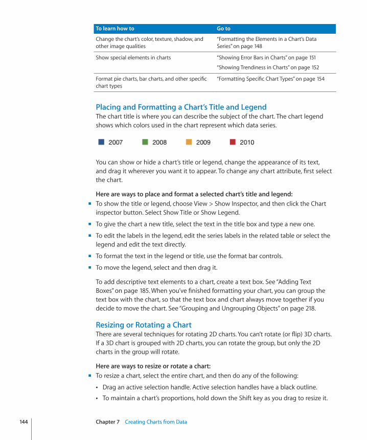
To learn how to Go to
Change the chart’s color, texture, shadow, and other image qualities
“Formatting the Elements in a Chart’s Data Series” on page 148
Show special elements in charts “Showing Error Bars in Charts” on page 151
“Showing Trendiness in Charts” on page 152
Format pie charts, bar charts, and other specific chart types
“Formatting Specific Chart Types” on page 154
Placing and Formatting a Chart’s Title and LegendThe chart title is where you can describe the subject of the chart. The chart legend shows which colors used in the chart represent which data series.
You can show or hide a chart’s title or legend, change the appearance of its text, and drag it wherever you want it to appear. To change any chart attribute, first select the chart.
Here are ways to place and format a selected chart’s title and legend:�To show the title or legend, choose View > Show Inspector, and then click the Chart m
inspector button. Select Show Title or Show Legend.
To give the chart a new title, select the text in the title box and type a new one. m
To edit the labels in the legend, edit the series labels in the related table or select the m
legend and edit the text directly.
To format the text in the legend or title, use the format bar controls. m
To move the legend, select and then drag it. m
To add descriptive text elements to a chart, create a text box. See “Adding Text Boxes” on page 185. When you’ve finished formatting your chart, you can group the text box with the chart, so that the text box and chart always move together if you decide to move the chart. See “Grouping and Ungrouping Objects” on page 218.
Resizing or Rotating a ChartThere are several techniques for rotating 2D charts. You can’t rotate (or flip) 3D charts. If a 3D chart is grouped with 2D charts, you can rotate the group, but only the 2D charts in the group will rotate.
Here are ways to resize or rotate a chart:�To resize a chart, select the entire chart, and then do any of the following: m
Drag an active selection handle. Active selection handles have a black outline. Â
To maintain a chart’s proportions, hold down the Shift key as you drag to resize it. Â
144 Chapter 7 Creating Charts from Data
Chapter 7 Creating Charts from Data 145
To resize a chart in one direction, drag a side handle instead of a corner handle. Â
To resize by specifying exact dimensions, click Inspector in the toolbar, and then Âclick the Metrics inspector button. In the Metrics inspector, you can specify a new width, height, and angle of rotation, and you can change the chart’s distance from the margins.
To rotate 2D charts, select the entire chart, and then do any of the following: m
Select the chart, hold down the Command key, move the pointer toward an active Âselection handle until it changes to a curved, double-headed arrow, and then drag a selection handle.
To rotate a chart in 45-degree increments, press the Shift and Command keys while Âdragging a selection handle.
Click Inspector in the toolbar, click the Metrics inspector button, and then drag the ÂRotate wheel or use the Angle controls to set the angle of the chart.
Pie charts can also be rotated using the Chart inspector. See “Rotating 2D Pie Charts” on page 158.
Formatting Chart AxesIn column charts, area charts, line charts, and bar charts, data points are plotted on one axis (the y-axis for column, area, and line charts; the x-axis for bar charts) and data sets are grouped on the other axis. The data point axis is called the value axis, and the data set axis is called the category axis.
In scatter charts, both the x and y axes are value axes. In 2-axis charts, there are two y axes—Value Axis (Y1) and Value Axis (Y2)—which can be formatted separately. For more details about 2-axis charts, see “Customizing 2-Axis and Mixed Charts” on page 161.
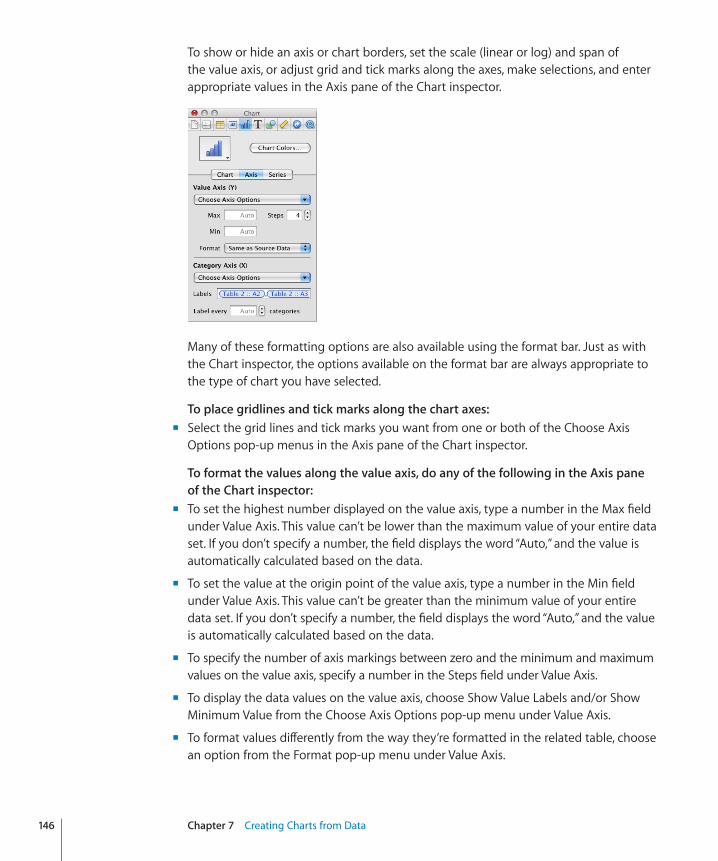
To show or hide an axis or chart borders, set the scale (linear or log) and span of the value axis, or adjust grid and tick marks along the axes, make selections, and enter appropriate values in the Axis pane of the Chart inspector.
Many of these formatting options are also available using the format bar. Just as with the Chart inspector, the options available on the format bar are always appropriate to the type of chart you have selected.
To place gridlines and tick marks along the chart axes:�Select the grid lines and tick marks you want from one or both of the Choose Axis m
Options pop-up menus in the Axis pane of the Chart inspector.
To format the values along the value axis, do any of the following in the Axis pane of the Chart inspector:�To set the highest number displayed on the value axis, type a number in the Max field m
under Value Axis. This value can’t be lower than the maximum value of your entire data set. If you don’t specify a number, the field displays the word “Auto,” and the value is automatically calculated based on the data.
To set the value at the origin point of the value axis, type a number in the Min field m
under Value Axis. This value can’t be greater than the minimum value of your entire data set. If you don’t specify a number, the field displays the word “Auto,” and the value is automatically calculated based on the data.
To specify the number of axis markings between zero and the minimum and maximum m
values on the value axis, specify a number in the Steps field under Value Axis.
To display the data values on the value axis, choose Show Value Labels and/or Show m
Minimum Value from the Choose Axis Options pop-up menu under Value Axis.
To format values differently from the way they’re formatted in the related table, choose m
an option from the Format pop-up menu under Value Axis.
146 Chapter 7 Creating Charts from Data
Chapter 7 Creating Charts from Data 147
Number:� Displays the data point value with no units, unless you specify them. To specify units, type them into the Suffix field. In the Decimals field, specify how many decimal places you want to appear, and then choose –100 or (100) from the adjacent pop-up menu to choose a style for displaying negative numbers. Select Separator if you want to show a thousands separator on the left side of the decimal.
Currency:� Displays the data point value as a monetary amount. Choose the currency unit symbol from the Symbol pop-up menu. In the Decimals field, specify how many decimal places you want to appear. To display negative values preceded by a minus sign or in parentheses, choose –100 or (100) from the pop-up menu. Select Separator if you want to show a thousands separator on the left side of the decimal.
Percentage:� Displays the data point value as divided by 100. In the Decimals field, specify how many decimal places you want to appear. To display negative values preceded by a minus sign or in parentheses, choose –100 or (100) from the pop-up menu. Select Separator if you want to show a thousands separator on the left side of the decimal.
Date and Time:� Displays data point values with a date and time format.
Duration:� Displays data point values as a unit of time (for example, seconds, minutes, or weeks).
Fraction:� Displays data point values less than 1 as one integer over another. (If your values are greater than 1, you won’t see any fractional representation of your data.) Select how accurately you want the fractions rounded in the Accuracy pop-up menu. Selecting an option such as Halves or Quarters represents the values as a portion of the total pie, rounded to the nearest division you selected.
Scientific: Displays data point values in scientific notation, where 10 raised to a power is represented as E+ an integer. In the Decimals field, specify how many decimal places you want to show.
Custom:� Select a custom number format you’ve already created, or create a new one. See “Using Your Own Formats for Displaying Values in Table Cells” on page 101 for more information.
To display category (data set) titles:� 1 Choose Show Categories from the Choose Axis Options pop-up menu under Category
Axis in the Axis pane of the Chart inspector.
2 To change the category labels, insert the pointer in the Labels field, do one of the following, and then click the Accept button (the green check) to save your changes:
To include a label, click the cell of the table where the label you want appears. ÂA reference to the cell is added to the Labels field.
To exclude a label, select the cell reference in the Label field and press the ÂDelete key.
3 To change the interval for label categories, do one or both of the following:
Type a value or use the stepper in the “Label every ... categories” field. For example, Âa value of 2 displays every other category title; a value of 3 displays every third category title, and so on.
Choose Show Last Category from the Choose Axis Options pop-up menu under ÂCategory Axis if you want the title of the last category to appear.
To add or hide an axis title:� 1 Choose Show Title from the Choose Axis Options pop-up menu under Value Axis or
Category Axis in the Axis pane of the Chart inspector.
2 On the chart, double-click the value title or category title that appears and type the title you want.
3 To format the title’s text attributes, use the controls in the format bar.
4 To hide a title, deselect the option in the same pop-up menus.
To set a linear, logarithmic, or percentage scale for the value axis:�Select Linear Scale, Log Scale, or Percentage Scale from the Choose Axis Options pop- m
up menu under Value Axis in the Axis pane of the Chart inspector.
Percentage scales are available only for 2D stacked bar, column, and area charts; linear and logarithmic scales are available only for 2D charts that aren’t stacked. 3D charts can only use a linear scale. (For pie charts, you display values as percentages by choosing Percentage from the Format pop-up menu under Labels.)
To change the color and texture of series elements, or to format data point symbols and value labels, use the Series pane of the Chart inspector. See “Formatting the Elements in a Chart’s Data Series” on page 148.
To learn about formatting options that are unique to a given chart type, see “Formatting Specific Chart Types” on page 154.
Formatting the Elements in a Chart’s Data SeriesYou can use a variety of visual effects to enhance the appearance of data series elements, such as bars (in column and bar charts), data point shapes (in line and scatter charts), and area shapes.
Pie wedges also represent a data series, but these have special formatting considerations. See “Customizing the Look of Pie Charts” on page 154 to learn more.
Many series formatting options are available in the format bar. When you select a series element in a chart, the items in the format bar change to provide appropriate options for formatting chart series elements. For example, you can click the Fill well in the format bar and quickly select a color to apply to the selected series element.
148 Chapter 7 Creating Charts from Data
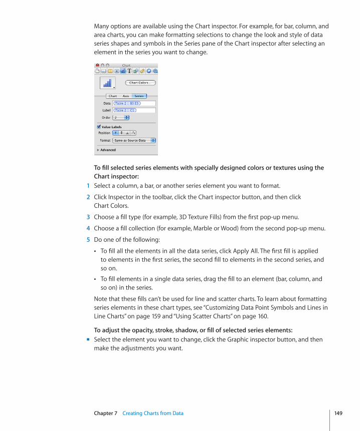
Chapter 7 Creating Charts from Data 149
Many options are available using the Chart inspector. For example, for bar, column, and area charts, you can make formatting selections to change the look and style of data series shapes and symbols in the Series pane of the Chart inspector after selecting an element in the series you want to change.
To fill selected series elements with specially designed colors or textures using the Chart inspector:�
1 Select a column, a bar, or another series element you want to format.
2 Click Inspector in the toolbar, click the Chart inspector button, and then click Chart Colors.
3 Choose a fill type (for example, 3D Texture Fills) from the first pop-up menu.
4 Choose a fill collection (for example, Marble or Wood) from the second pop-up menu.
5 Do one of the following:
To fill all the elements in all the data series, click Apply All. The first fill is applied Âto elements in the first series, the second fill to elements in the second series, and so on.
To fill elements in a single data series, drag the fill to an element (bar, column, and Âso on) in the series.
Note that these fills can’t be used for line and scatter charts. To learn about formatting series elements in these chart types, see “Customizing Data Point Symbols and Lines in Line Charts” on page 159 and “Using Scatter Charts” on page 160.
To adjust the opacity, stroke, shadow, or fill of selected series elements:Select the element you want to change, click the Graphic inspector button, and then m
make the adjustments you want.
When adjusting the opacity and fill, note that dragging the Opacity slider at the bottom of the Graphic inspector changes the opacity of the chart as a whole. To format only a selected series, select it, and then adjust the opacity of the color fill, gradient fill, or tinted image fill, as needed. For more details, see “Adjusting Opacity” on page 224 and “Filling Objects with Colors or Images” on page 225.
To learn about using one of your own images as a fill, see “Filling an Object with an Image” on page 228.
To learn about changing the look of the line around an element, see “Changing the Style of Borders” on page 221.
To learn about changing shadows, see “Adding Shadows” on page 223.
To show and format data point labels for the selected series:� 1 Click Series in the Chart inspector.
2 Select Value Labels.
3 To position the labels, click one of the Position buttons.
4 To format values differently from the way they’re formatted in the related table, select an option from the Format pop-up menu under Value Axis.
Number:� Displays the data point value with no units, unless you specify them. To specify units, type them into the Suffix field. In the Decimals field, specify how many decimal places you want to appear, and then choose –100 or (100) from the adjacent pop-up menu to choose a style for displaying negative numbers. Select Separator if you want to show a thousands separator on the left side of the decimal.
Currency:� Displays the data point value as a monetary amount. Choose the currency unit symbol from the Symbol pop-up menu. In the Decimals field, specify how many decimal places you want to appear. To display negative values preceded by a minus sign or in parentheses, choose –100 or (100) from the pop-up menu. Select Separator if you want to show a thousands separator on the left side of the decimal.
Percentage:� Displays the data point value as divided by 100. In the Decimals field, specify how many decimal places you want to appear. To display negative values preceded by a minus sign or in parentheses, choose –100 or (100) from the pop-up menu. Select Separator if you want to show a thousands separator on the left side of the decimal.
Date and Time:� Displays data point values with a date and time format.
Duration:� Displays data point values as a unit of time (for example, seconds, minutes, or weeks).
150 Chapter 7 Creating Charts from Data
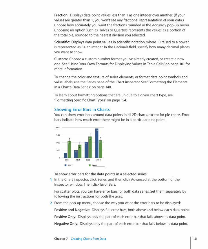
Chapter 7 Creating Charts from Data 151
Fraction:� Displays data point values less than 1 as one integer over another. (If your values are greater than 1, you won’t see any fractional representation of your data.) Choose how accurately you want the fractions rounded in the Accuracy pop-up menu. Choosing an option such as Halves or Quarters represents the values as a portion of the total pie, rounded to the nearest division you selected.
Scientific: Displays data point values in scientific notation, where 10 raised to a power is represented as E+ an integer. In the Decimals field, specify how many decimal places you want to show.
Custom:� Choose a custom number format you’ve already created, or create a new one. See “Using Your Own Formats for Displaying Values in Table Cells” on page 101 for more information.
To change the color and texture of series elements, or format data point symbols and value labels, use the Series pane of the Chart inspector. See “Formatting the Elements in a Chart’s Data Series” on page 148.
To learn about formatting options that are unique to a given chart type, see “Formatting Specific Chart Types” on page 154.
Showing Error Bars in ChartsYou can show error bars around data points in all 2D charts, except for pie charts. Error bars indicate how much error there might be in a particular data point.
To show error bars for the data points in a selected series:� 1 In the Chart inspector, click Series, and then click Advanced at the bottom of the
Inspector window. Then click Error Bars.
For scatter plots, you can have error bars for both data series. Set them separately by following the instructions for both the axes.
2 From the pop-up menu, choose the way you want the error bars to be displayed:
Positive and Negative:� Displays full error bars, both above and below each data point.
Positive Only:� Displays only the part of each error bar that falls above its data point.
Negative Only:� Displays only the part of each error bar that falls below its data point.
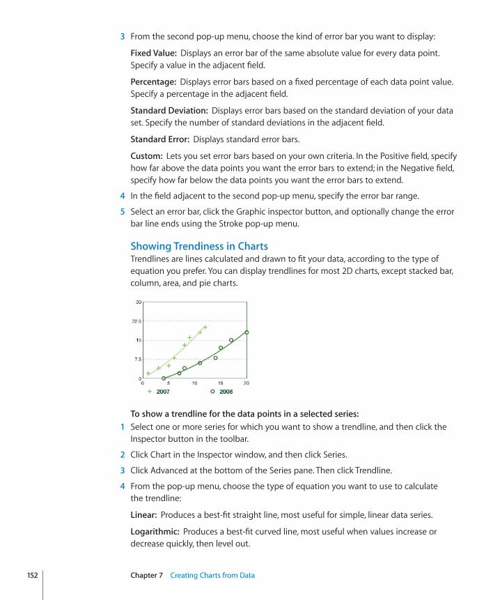
3 From the second pop-up menu, choose the kind of error bar you want to display:
Fixed Value:� Displays an error bar of the same absolute value for every data point. Specify a value in the adjacent field.
Percentage:� Displays error bars based on a fixed percentage of each data point value. Specify a percentage in the adjacent field.
Standard Deviation:� Displays error bars based on the standard deviation of your data set. Specify the number of standard deviations in the adjacent field.
Standard Error:� Displays standard error bars.
Custom:� Lets you set error bars based on your own criteria. In the Positive field, specify how far above the data points you want the error bars to extend; in the Negative field, specify how far below the data points you want the error bars to extend.
4 In the field adjacent to the second pop-up menu, specify the error bar range.
5 Select an error bar, click the Graphic inspector button, and optionally change the error bar line ends using the Stroke pop-up menu.
Showing Trendiness in ChartsTrendlines are lines calculated and drawn to fit your data, according to the type of equation you prefer. You can display trendlines for most 2D charts, except stacked bar, column, area, and pie charts.
To show a trendline for the data points in a selected series:� 1 Select one or more series for which you want to show a trendline, and then click the
Inspector button in the toolbar.
2 Click Chart in the Inspector window, and then click Series.
3 Click Advanced at the bottom of the Series pane. Then click Trendline.
4 From the pop-up menu, choose the type of equation you want to use to calculate the trendline:
Linear:� Produces a best-fit straight line, most useful for simple, linear data series.
Logarithmic:� Produces a best-fit curved line, most useful when values increase or decrease quickly, then level out.
152 Chapter 7 Creating Charts from Data
Chapter 7 Creating Charts from Data 153
Polynomial:� Produces a curved line that has hills and valleys to show where values rise or fall. Specify the order of polynomial you want to use in the Order field; order 4 produces as many as 3 hills or valleys.
Power:� Produces a curved line for use when you want to compare measurements that increase at a specific rate. Power can’t be used with data that contains zero or negative values.
Exponential:� Produces a curved line for use when values rise or fall at increasingly higher rates. Exponential can’t be used with data that contains zero or negative values.
Moving Average:� Produces a trendline using the number of data points you specify in the Period field, averages them, and uses the average value as a trendline point.
5 To see the equation that describes a trendline, select the line, and then select Show Equation. You can drag this equation to wherever you want it to appear on the sheet.
6 To see the R-squared value that was used to calculate a trendline, select the line, and then select Show R^2 Value. You can drag this number to wherever you want it to appear on the sheet.
7 To display a label for a trendline, select the trendline and then select Label. Type a label in the adjacent field.
8 To change the line color or thickness of a trendline, select the trendline, and then click the Graphic button in the Inspector window. Make adjustments using the Stroke controls.
Formatting the Text of Chart Titles, Labels, and LegendsYou can change the size and appearance of chart and axis titles, axis labels, data point labels, and legends.
To format the text of labels and legends:� 1 Depending on which text you want to format, select the appropriate item:
To format all chart titles and labels (excluding the chart legend), click the chart to change all the text to your font and color choices.
To format the text for all data points in one series only, select the text box for one data point in the series.
To format the text in an axis label, select the text.
To format the text for all series labels, select the series label box.
To change the text in a chart legend, select the legend.
2 Use the format bar controls to format the selected text.
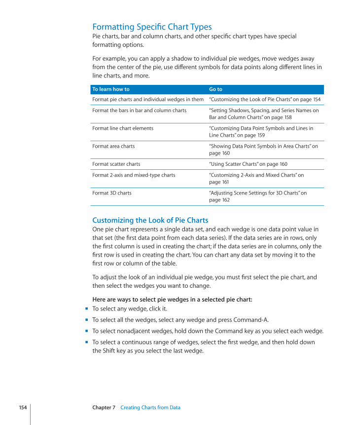
Formatting Specific Chart TypesPie charts, bar and column charts, and other specific chart types have special formatting options.
For example, you can apply a shadow to individual pie wedges, move wedges away from the center of the pie, use different symbols for data points along different lines in line charts, and more.
To learn how to Go to
Format pie charts and individual wedges in them “Customizing the Look of Pie Charts” on page 154
Format the bars in bar and column charts “Setting Shadows, Spacing, and Series Names on Bar and Column Charts” on page 158
Format line chart elements “Customizing Data Point Symbols and Lines in Line Charts” on page 159
Format area charts “Showing Data Point Symbols in Area Charts” on page 160
Format scatter charts “Using Scatter Charts” on page 160
Format 2-axis and mixed-type charts “Customizing 2-Axis and Mixed Charts” on page 161
Format 3D charts “Adjusting Scene Settings for 3D Charts” on page 162
Customizing the Look of Pie ChartsOne pie chart represents a single data set, and each wedge is one data point value in that set (the first data point from each data series). If the data series are in rows, only the first column is used in creating the chart; if the data series are in columns, only the first row is used in creating the chart. You can chart any data set by moving it to the first row or column of the table.
To adjust the look of an individual pie wedge, you must first select the pie chart, and then select the wedges you want to change.
Here are ways to select pie wedges in a selected pie chart:�To select any wedge, click it. m
To select all the wedges, select any wedge and press Command-A. m
To select nonadjacent wedges, hold down the Command key as you select each wedge. m
To select a continuous range of wedges, select the first wedge, and then hold down m
the Shift key as you select the last wedge.
154 Chapter 7 Creating Charts from Data
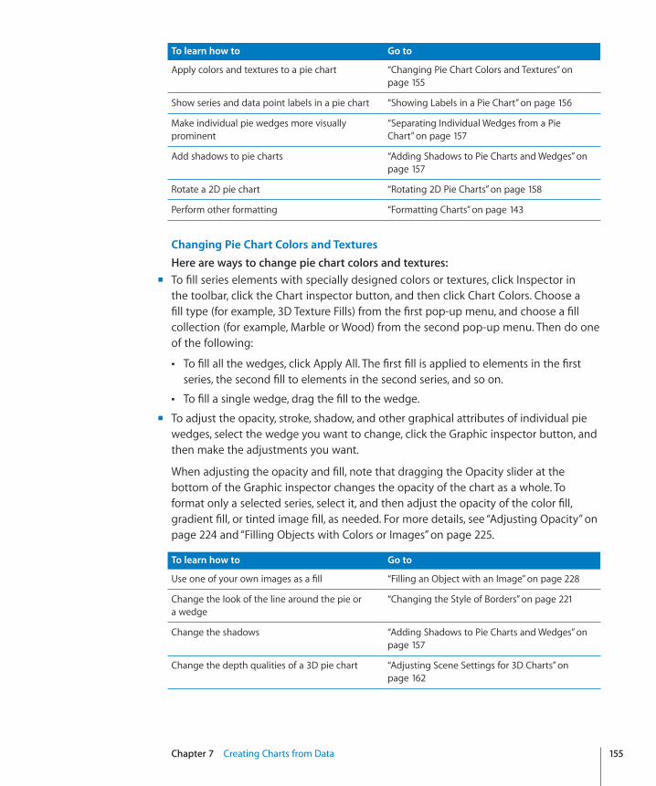
Chapter 7 Creating Charts from Data 155
To learn how to Go to
Apply colors and textures to a pie chart “Changing Pie Chart Colors and Textures” on page 155
Show series and data point labels in a pie chart “Showing Labels in a Pie Chart” on page 156
Make individual pie wedges more visually prominent
“Separating Individual Wedges from a Pie Chart” on page 157
Add shadows to pie charts “Adding Shadows to Pie Charts and Wedges” on page 157
Rotate a 2D pie chart “Rotating 2D Pie Charts” on page 158
Perform other formatting “Formatting Charts” on page 143
Changing Pie Chart Colors and TexturesHere are ways to change pie chart colors and textures:�To fill series elements with specially designed colors or textures, click Inspector in m
the toolbar, click the Chart inspector button, and then click Chart Colors. Choose a fill type (for example, 3D Texture Fills) from the first pop-up menu, and choose a fill collection (for example, Marble or Wood) from the second pop-up menu. Then do one of the following:
To fill all the wedges, click Apply All. The first fill is applied to elements in the first Âseries, the second fill to elements in the second series, and so on.
To fill a single wedge, drag the fill to the wedge. Â
To adjust the opacity, stroke, shadow, and other graphical attributes of individual pie m
wedges, select the wedge you want to change, click the Graphic inspector button, and then make the adjustments you want.
When adjusting the opacity and fill, note that dragging the Opacity slider at the bottom of the Graphic inspector changes the opacity of the chart as a whole. To format only a selected series, select it, and then adjust the opacity of the color fill, gradient fill, or tinted image fill, as needed. For more details, see “Adjusting Opacity” on page 224 and “Filling Objects with Colors or Images” on page 225.
To learn how to Go to
Use one of your own images as a fill “Filling an Object with an Image” on page 228
Change the look of the line around the pie or a wedge
“Changing the Style of Borders” on page 221
Change the shadows “Adding Shadows to Pie Charts and Wedges” on page 157
Change the depth qualities of a 3D pie chart “Adjusting Scene Settings for 3D Charts” on page 162
Showing Labels in a Pie ChartTo show series and data point labels in pie charts, use the Chart inspector.
To show series names or data point labels in a pie chart:� 1 Select the chart or individual pie wedges for which you want to show a label or
series name.
2 Click Inspector in the toolbar, and then click the Chart inspector button.
3 Select Labels, and then drag the Position slider to place the data point label closer to—or farther away from—the center of the pie. Alternatively, specify a value in the field to set the wedge’s distance from the center of the pie as a percentage of the pie’s radius.
You can also use the Labels slider in the format bar to position labels.
4 To display the values in a particular format, make a selection from the Format pop-up menu and adjust the options:
Number:� Displays the data point value with no units, unless you specify them. To specify units, type them into the Suffix field. In the Decimals field, specify how many decimal places you want to appear, and then choose –100 or (100) from the adjacent pop-up menu to choose a style for displaying negative numbers. Select Separator if you want to show a thousands separator on the left side of the decimal.
Currency:� Displays the data point value as a monetary amount. Choose the currency unit symbol from the Symbol pop-up menu. In the Decimals field, specify how many decimal places you want to appear. To display negative values preceded by a minus sign or in parentheses, choose –100 or (100) from the pop-up menu. Select Separator if you want to show a thousands separator on the left side of the decimal.
Percentage:� Displays the data point value as divided by 100. In the Decimals field, specify how many decimal places you want to appear. To display negative values preceded by a minus sign or in parentheses, choose –100 or (100) from the pop-up menu. Select Separator if you want to show a thousands separator on the left side of the decimal.
Date and Time:� Displays data point values with a date and time format.
Duration:� Displays data point values as a unit of time (for example, seconds, minutes, or weeks).
Fraction:� Displays data point values less than 1 as one integer over another. (If your values are greater than 1, you won’t see any fractional representation of your data.) Choose how accurately you want the fractions rounded in the Accuracy pop-up menu. Choosing an option such as Halves or Quarters represents the values as a portion of the total pie, rounded to the nearest division you selected.
156 Chapter 7 Creating Charts from Data
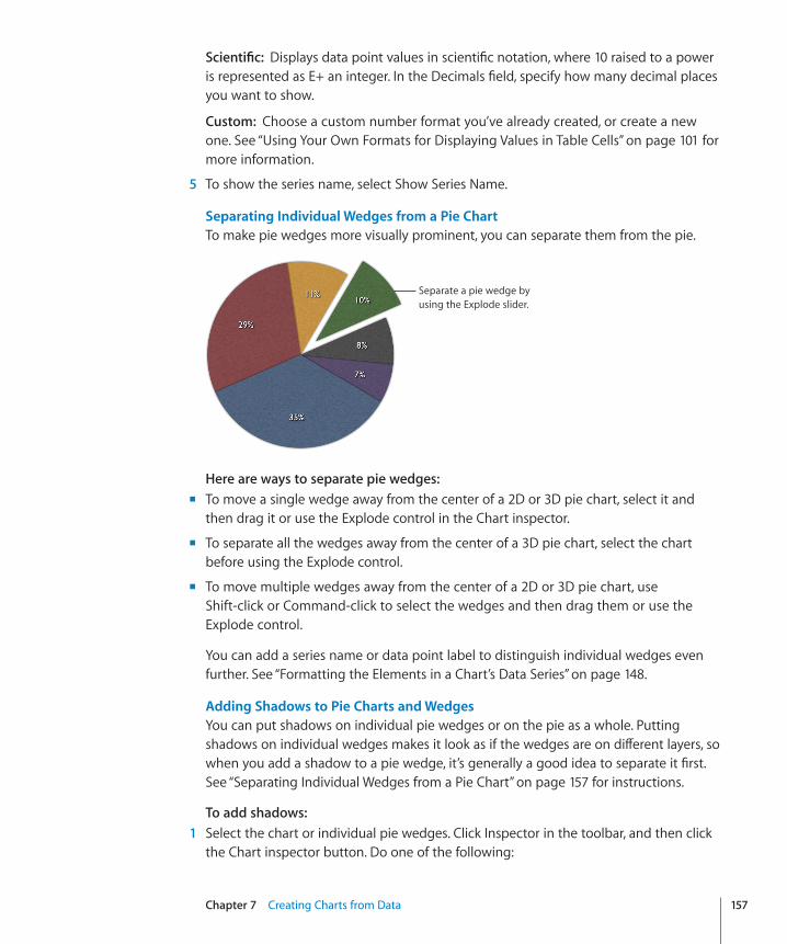
Chapter 7 Creating Charts from Data 157
Scientific: Displays data point values in scientific notation, where 10 raised to a power is represented as E+ an integer. In the Decimals field, specify how many decimal places you want to show.
Custom:� Choose a custom number format you’ve already created, or create a new one. See “Using Your Own Formats for Displaying Values in Table Cells” on page 101 for more information.
5 To show the series name, select Show Series Name.
Separating Individual Wedges from a Pie ChartTo make pie wedges more visually prominent, you can separate them from the pie.
Separate a pie wedge by using the Explode slider.
Here are ways to separate pie wedges:�To move a single wedge away from the center of a 2D or 3D pie chart, select it and m
then drag it or use the Explode control in the Chart inspector.
To separate all the wedges away from the center of a 3D pie chart, select the chart m
before using the Explode control.
To move multiple wedges away from the center of a 2D or 3D pie chart, use m
Shift-click or Command-click to select the wedges and then drag them or use the Explode control.
You can add a series name or data point label to distinguish individual wedges even further. See “Formatting the Elements in a Chart’s Data Series” on page 148.
Adding Shadows to Pie Charts and WedgesYou can put shadows on individual pie wedges or on the pie as a whole. Putting shadows on individual wedges makes it look as if the wedges are on different layers, so when you add a shadow to a pie wedge, it’s generally a good idea to separate it first. See “Separating Individual Wedges from a Pie Chart” on page 157 for instructions.
To add shadows:� 1 Select the chart or individual pie wedges. Click Inspector in the toolbar, and then click
the Chart inspector button. Do one of the following:
To add shadows to individually selected wedges, choose Individual from the ÂShadow pop-up menu.
To add a shadow to the chart as a whole, choose Group from the Shadow Âpop-up menu.
You can also use the Shadow pop-up menu in the format bar.
2 To set shadow attributes, use the Graphic inspector. See “Adding Shadows” on page 223 for instructions.
Rotating 2D Pie ChartsHere are ways to rotate a pie chart:�Select the chart, click Inspector in the toolbar, click the Chart inspector button, and m
then use the Rotation Angle wheel or field.
Click Inspector in the toolbar, click the Metrics inspector button, and then drag the m
Rotate wheel or use the Angle controls to set the angle of the chart.
Select the chart, hold down the Command key and move the pointer toward an active m
selection handle until it changes to a curved, double-headed arrow, and then drag a selection handle.
To rotate the chart in 45-degree increments, press the Shift and Command keys while m
dragging a selection handle or the Rotate wheel.
Setting Shadows, Spacing, and Series Names on Bar and Column ChartsOn bar and column charts, you can adjust the distance between the sets of bars or columns (data sets). On charts where the data sets aren’t stacked, you can also adjust the distance between the bars or columns (individual data sets). You can also apply shadows to individual data series or to the entire chart.
On bar and column charts that are not stacked, you can also opt to show the series names, or Labels.
To customize bars and column charts:� 1 Select a bar or column chart.
2 Click Inspector in the toolbar, click the Chart inspector button, and then click Chart.
3 To change the space between bars or categories, do one of the following:
To change the space between bars, type a value (or click the arrows) in the “Gap Âbetween bars” field.
To change the space between categories (on unstacked charts), specify a value in Âthe “Gap between sets” field.
The value is the percentage of the bar thickness. Decreasing the space between the bars makes them thicker. You can also move the pointer near a bar edge until it becomes a double-headed arrow, and then drag to make the bars thicker or thinner.
158 Chapter 7 Creating Charts from Data
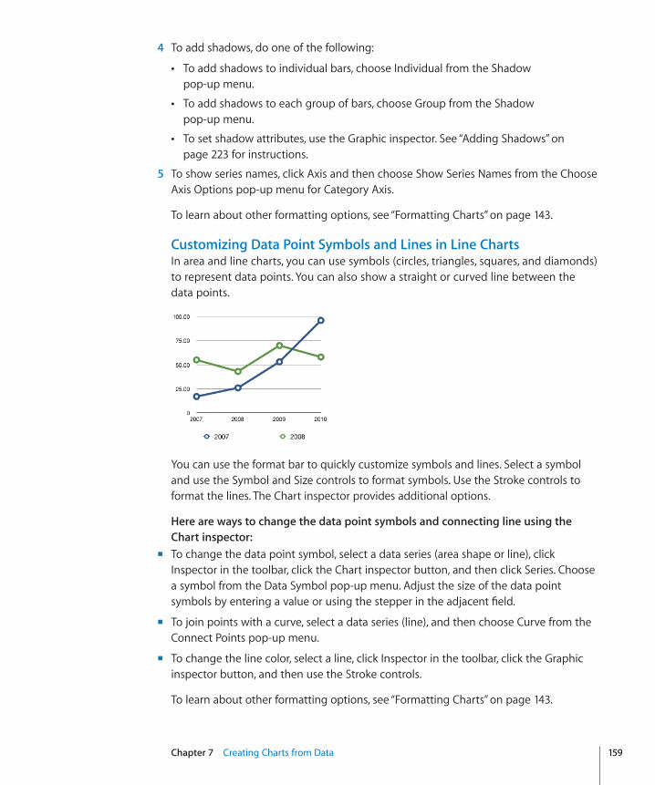
Chapter 7 Creating Charts from Data 159
4 To add shadows, do one of the following:
To add shadows to individual bars, choose Individual from the Shadow Âpop-up menu.
To add shadows to each group of bars, choose Group from the Shadow Âpop-up menu.
To set shadow attributes, use the Graphic inspector. See “ Â Adding Shadows” on page 223 for instructions.
5 To show series names, click Axis and then choose Show Series Names from the Choose Axis Options pop-up menu for Category Axis.
To learn about other formatting options, see “Formatting Charts” on page 143.
Customizing Data Point Symbols and Lines in Line ChartsIn area and line charts, you can use symbols (circles, triangles, squares, and diamonds) to represent data points. You can also show a straight or curved line between the data points.
You can use the format bar to quickly customize symbols and lines. Select a symbol and use the Symbol and Size controls to format symbols. Use the Stroke controls to format the lines. The Chart inspector provides additional options.
Here are ways to change the data point symbols and connecting line using the Chart inspector:�To change the data point symbol, select a data series (area shape or line), click m
Inspector in the toolbar, click the Chart inspector button, and then click Series. Choose a symbol from the Data Symbol pop-up menu. Adjust the size of the data point symbols by entering a value or using the stepper in the adjacent field.
To join points with a curve, select a data series (line), and then choose Curve from the m
Connect Points pop-up menu.
To change the line color, select a line, click Inspector in the toolbar, click the Graphic m
inspector button, and then use the Stroke controls.
To learn about other formatting options, see “Formatting Charts” on page 143.
Showing Data Point Symbols in Area ChartsIn area charts, you can use symbols (circles, triangles, squares, and diamonds) to represent data points.
You can use the format bar to quickly customize symbols. Select a symbol and use the Symbol and Size controls to format symbols. You can also use the Chart inspector.
To show data point symbols using the Chart inspector:� 1 Select a data series (area shape), click Inspector in the toolbar, click the Chart inspector
button, and then click Series.
2 Choose a symbol from the Data Symbol pop-up menu.
3 Adjust the size of the data point symbols by entering a value or using the stepper in the adjacent field.
To learn about other formatting options, see “Formatting Charts” on page 143.
Using Scatter ChartsScatter charts display data differently from the other kinds of charts. They require at least two columns or rows of data to plot values for a single data series. To show multiple data series, you use additional two-column (or two-row) pairs.
Each pair of values determines the position of one data point. The first data value in the pair is the x-axis of the point. The second data value is the y-axis of the point. If you’ve already created a chart with data points that don’t occur in pairs, and then you change your chart to a scatter chart, Numbers may not plot the data as you expect. Depending on how the data is arranged in the table, it may not be possible to create any plot at all. Make sure you have entered x and y point values for each data series you want to plot before choosing to create a scatter chart.
When you choose a scatter chart, the series button appears as a gear in the top left corner of the data table overlay. You can use a single column (or row) of data as the x value for multiple columns (or rows) of y values by clicking the gear button and selecting Share X Values. Use the same button to switch between using rows or columns as data series in your chart.
Before you can change the look of data point symbols or lines, you must select a symbol or line of interest.
You can use the format bar to quickly customize symbols and lines. Select a symbol and use the Symbol and Size controls to format symbols. Use the Stroke controls to format the lines. The Chart inspector offers additional options.
160 Chapter 7 Creating Charts from Data
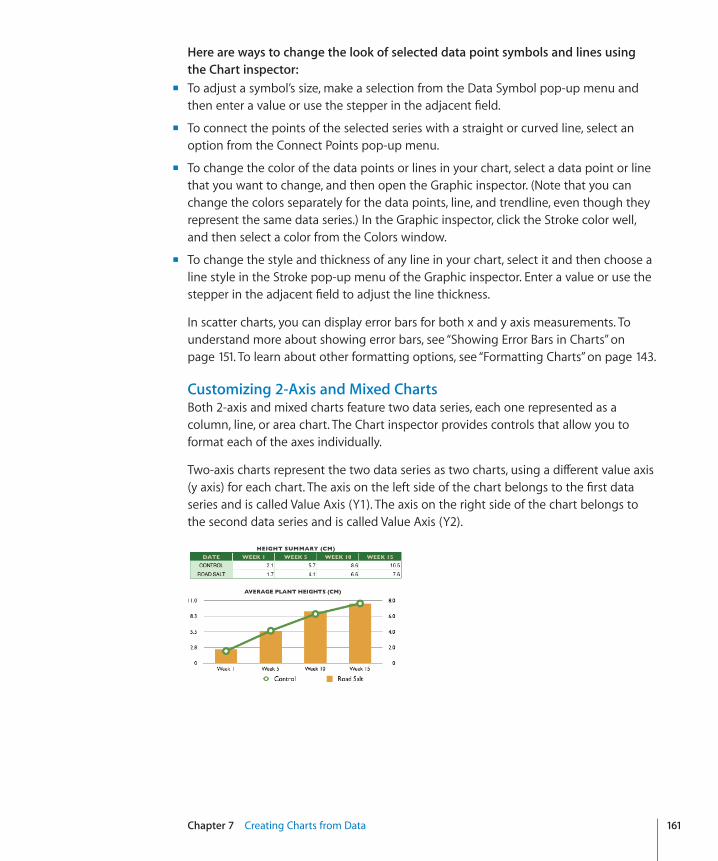
Chapter 7 Creating Charts from Data 161
Here are ways to change the look of selected data point symbols and lines using the Chart inspector:�To adjust a symbol’s size, make a selection from the Data Symbol pop-up menu and m
then enter a value or use the stepper in the adjacent field.
To connect the points of the selected series with a straight or curved line, select an m
option from the Connect Points pop-up menu.
To change the color of the data points or lines in your chart, select a data point or line m
that you want to change, and then open the Graphic inspector. (Note that you can change the colors separately for the data points, line, and trendline, even though they represent the same data series.) In the Graphic inspector, click the Stroke color well, and then select a color from the Colors window.
To change the style and thickness of any line in your chart, select it and then choose a m
line style in the Stroke pop-up menu of the Graphic inspector. Enter a value or use the stepper in the adjacent field to adjust the line thickness.
In scatter charts, you can display error bars for both x and y axis measurements. To understand more about showing error bars, see “Showing Error Bars in Charts” on page 151. To learn about other formatting options, see “Formatting Charts” on page 143.
Customizing 2-Axis and Mixed ChartsBoth 2-axis and mixed charts feature two data series, each one represented as a column, line, or area chart. The Chart inspector provides controls that allow you to format each of the axes individually.
Two-axis charts represent the two data series as two charts, using a different value axis (y axis) for each chart. The axis on the left side of the chart belongs to the first data series and is called Value Axis (Y1). The axis on the right side of the chart belongs to the second data series and is called Value Axis (Y2).
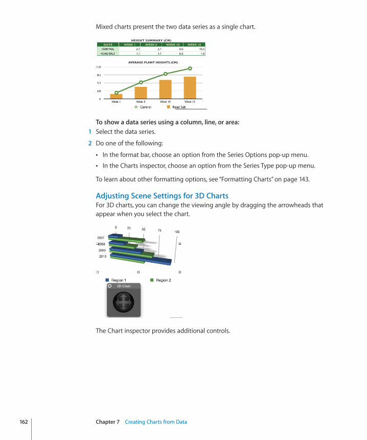
Mixed charts present the two data series as a single chart.
To show a data series using a column, line, or area:� 1 Select the data series.
2 Do one of the following:
In the format bar, choose an option from the Series Options pop-up menu. Â
In the Charts inspector, choose an option from the Series Type pop-up menu. Â
To learn about other formatting options, see “Formatting Charts” on page 143.
Adjusting Scene Settings for 3D ChartsFor 3D charts, you can change the viewing angle by dragging the arrowheads that appear when you select the chart.
The Chart inspector provides additional controls.
162 Chapter 7 Creating Charts from Data
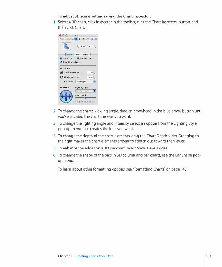
Chapter 7 Creating Charts from Data 163
To adjust 3D scene settings using the Chart inspector:� 1 Select a 3D chart, click Inspector in the toolbar, click the Chart inspector button, and
then click Chart.
2 To change the chart’s viewing angle, drag an arrowhead in the blue arrow button until you’ve situated the chart the way you want.
3 To change the lighting angle and intensity, select an option from the Lighting Style pop-up menu that creates the look you want.
4 To change the depth of the chart elements, drag the Chart Depth slider. Dragging to the right makes the chart elements appear to stretch out toward the viewer.
5 To enhance the edges on a 3D pie chart, select Show Bevel Edges.
6 To change the shape of the bars in 3D column and bar charts, use the Bar Shape pop-up menu.
To learn about other formatting options, see “Formatting Charts” on page 143.
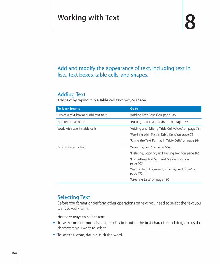
164
Add and modify the appearance of text, including text in lists, text boxes, table cells, and shapes.
Adding TextAdd text by typing it in a table cell, text box, or shape.
To learn how to Go to
Create a text box and add text to it “Adding Text Boxes” on page 185
Add text to a shape “Putting Text Inside a Shape” on page 186
Work with text in table cells “Adding and Editing Table Cell Values” on page 78
“Working with Text in Table Cells” on page 79
“Using the Text Format in Table Cells” on page 99
Customize your text “Selecting Text” on page 164
“Deleting, Copying, and Pasting Text” on page 165
“Formatting Text Size and Appearance” on page 165
“Setting Text Alignment, Spacing, and Color” on page 172
“Creating Lists” on page 180
Selecting TextBefore you format or perform other operations on text, you need to select the text you want to work with.
Here are ways to select text:�To select one or more characters, click in front of the first character and drag across the m
characters you want to select.
To select a word, double-click the word. m
8Working with Text
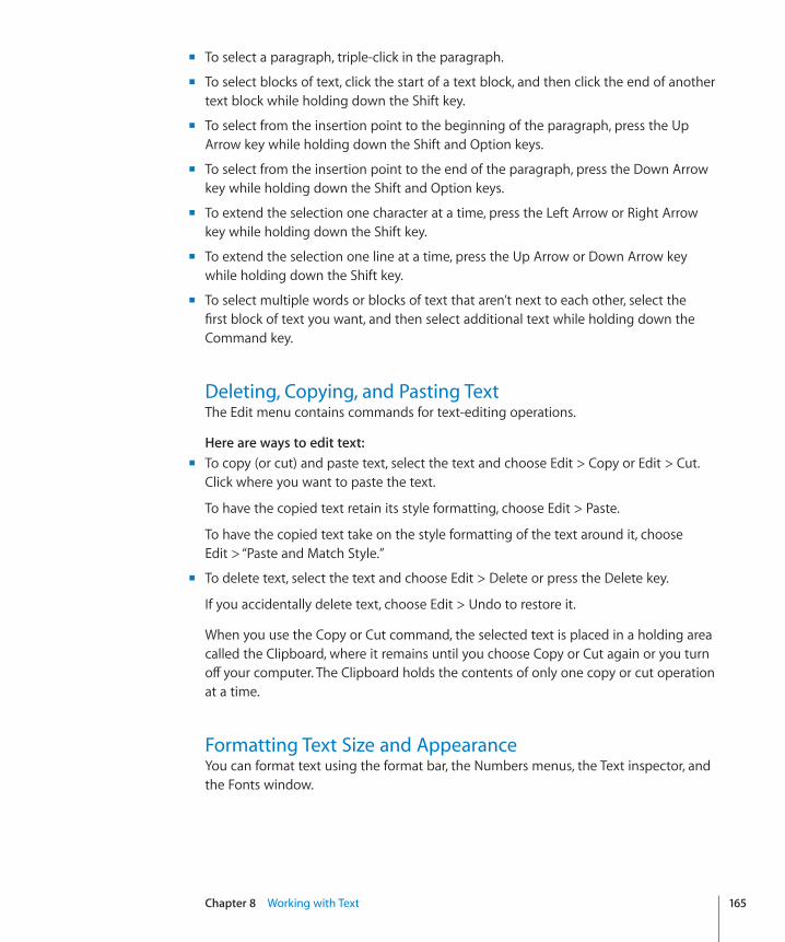
Chapter 8 Working with Text 165
To select a paragraph, triple-click in the paragraph. m
To select blocks of text, click the start of a text block, and then click the end of another m
text block while holding down the Shift key.
To select from the insertion point to the beginning of the paragraph, press the Up m
Arrow key while holding down the Shift and Option keys.
To select from the insertion point to the end of the paragraph, press the Down Arrow m
key while holding down the Shift and Option keys.
To extend the selection one character at a time, press the Left Arrow or Right Arrow m
key while holding down the Shift key.
To extend the selection one line at a time, press the Up Arrow or Down Arrow key m
while holding down the Shift key.
To select multiple words or blocks of text that aren’t next to each other, select the m
first block of text you want, and then select additional text while holding down the Command key.
Deleting, Copying, and Pasting TextThe Edit menu contains commands for text-editing operations.
Here are ways to edit text:�To copy (or cut) and paste text, select the text and choose Edit > Copy or Edit > Cut. m
Click where you want to paste the text.
To have the copied text retain its style formatting, choose Edit > Paste.
To have the copied text take on the style formatting of the text around it, choose Edit > “Paste and Match Style.”
To delete text, select the text and choose Edit > Delete or press the Delete key. m
If you accidentally delete text, choose Edit > Undo to restore it.
When you use the Copy or Cut command, the selected text is placed in a holding area called the Clipboard, where it remains until you choose Copy or Cut again or you turn off your computer. The Clipboard holds the contents of only one copy or cut operation at a time.
Formatting Text Size and AppearanceYou can format text using the format bar, the Numbers menus, the Text inspector, and the Fonts window.
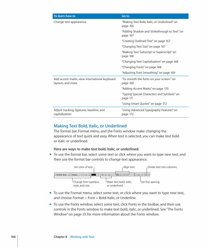
To learn how to Go to
Change text appearance “Making Text Bold, Italic, or Underlined” on page 166
“Adding Shadow and Strikethrough to Text” on page 167
“Creating Outlined Text” on page 167
“Changing Text Size” on page 167
“Making Text Subscript or Superscript” on page 168
“Changing Text Capitalization” on page 168
“Changing Fonts” on page 168
“Adjusting Font Smoothing” on page 169
Add accent marks, view international keyboard layouts, and more
“To smooth the fonts on your screen:” on page 169
“Adding Accent Marks” on page 170
“Typing Special Characters and Symbols” on page 171
“Using Smart Quotes” on page 172
Adjust tracking, ligatures, baseline, and capitalization
“Using Advanced Typography Features” on page 172
Making Text Bold, Italic, or UnderlinedThe format bar, Format menu, and the Fonts window make changing the appearance of text quick and easy. When text is selected, you can make text bold or italic or underlined.
Here are ways to make text bold, italic, or underlined:�To use the format bar, select some text or click where you want to type new text, and m
then use the format bar controls to change text appearance.
Change font typeface, style, and size.
Set color of text.
Make text bold, italic,or underlined.
Align text.
Set line spacing.
Divide text into columns.
To use the Format menu, select some text, or click where you want to type new text, m
and choose Format > Font > Bold, Italic, or Underline.
To use the Fonts window, select some text, click Fonts in the toolbar, and then use m
controls in the Fonts window to make text bold, italic, or underlined. See “The Fonts Window” on page 25 for more information about the Fonts window.
166 Chapter 8 Working with Text
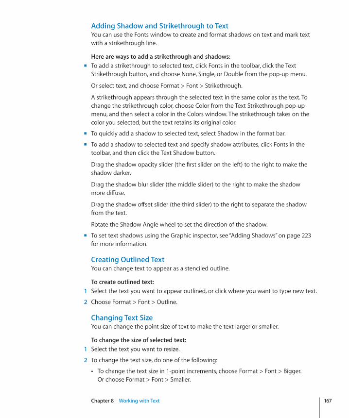
Chapter 8 Working with Text 167
Adding Shadow and Strikethrough to TextYou can use the Fonts window to create and format shadows on text and mark text with a strikethrough line.
Here are ways to add a strikethrough and shadows:�To add a strikethrough to selected text, click Fonts in the toolbar, click the Text m
Strikethrough button, and choose None, Single, or Double from the pop-up menu.
Or select text, and choose Format > Font > Strikethrough.
A strikethrough appears through the selected text in the same color as the text. To change the strikethrough color, choose Color from the Text Strikethrough pop-up menu, and then select a color in the Colors window. The strikethrough takes on the color you selected, but the text retains its original color.
To quickly add a shadow to selected text, select Shadow in the format bar. m
To add a shadow to selected text and specify shadow attributes, click Fonts in the m
toolbar, and then click the Text Shadow button.
Drag the shadow opacity slider (the first slider on the left) to the right to make the shadow darker.
Drag the shadow blur slider (the middle slider) to the right to make the shadow more diffuse.
Drag the shadow offset slider (the third slider) to the right to separate the shadow from the text.
Rotate the Shadow Angle wheel to set the direction of the shadow.
To set text shadows using the Graphic inspector, see “ m Adding Shadows” on page 223 for more information.
Creating Outlined TextYou can change text to appear as a stenciled outline.
To create outlined text:� 1 Select the text you want to appear outlined, or click where you want to type new text.
2 Choose Format > Font > Outline.
Changing Text SizeYou can change the point size of text to make the text larger or smaller.
To change the size of selected text:� 1 Select the text you want to resize.
2 To change the text size, do one of the following:
To change the text size in 1-point increments, choose Format > Font > Bigger. ÂOr choose Format > Font > Smaller.
You can also use the Text Size pop-up menu in the format bar.
To specify a precise size for selected text, click Fonts in the toolbar and use Âthe Size controls in the Fonts window. See “Changing Fonts” on page 168 for more information.
You can also add Bigger and Smaller icons to the toolbar. Choose View > Customize Toolbar, drag the icons to the toolbar, and then click Done.
Making Text Subscript or SuperscriptYou can raise or lower text from its baseline.
To make text subscript or superscript:� 1 Select the text you want to raise or lower, or click where you want to type new text.
2 To create a subscript or superscript that has a smaller font size than the text it accompanies, choose Format > Font > Baseline > Subscript. Or choose Format > Font > Baseline > Superscript.
To raise or lower text relative to the other text on the same line, choose Raise or Lower from the Baseline submenu.
To restore text to the same baseline as the body text, choose Use Default from the Baseline submenu.
You can add Subscript and Superscript icons to the toolbar. Choose View > Customize Toolbar, drag the icons to the toolbar, and then click Done.
Changing Text CapitalizationYou can quickly make blocks of text all uppercase or lowercase or format text as a title.
To change text capitalization:� 1 Select the text you want to change, or click where you want to type new text.
2 Choose Format > Font > Capitalization and choose an option from the submenu.
Choose All Caps to change the text to capitals.
Choose Small Caps to change the text to smaller capitals with larger capitals for uppercase letters.
Choose Title to change the text to a title format, which capitalizes the first letter of each word.
Choose None to avoid automatic capitalization.
Changing FontsWhen text is selected, quickly change font family, type, size, color, and background color using the controls in the format bar.
168 Chapter 8 Working with Text
Chapter 8 Working with Text 169
The Fonts window gives you extensive control over fonts. Use size controls and typography settings to customize the appearance of your text.
To modify the font of selected text using the Fonts window:� 1 Click Fonts in the toolbar.
2 In the Fonts window, select a font style in the Family column and then select the typeface in the Typeface column.
If you don’t see all the font families you know are installed on your computer, select All Fonts in the Collections column or type the name of the font you are looking for in the search field at the bottom of the Fonts window.
A preview of the selected font appears in the preview pane at the top of the Fonts window. If you don’t see a preview pane, choose Show Preview from the Action pop-up menu in the lower-left corner of the Fonts window.
3 Adjust the font size using the size slider or other size controls.
4 Adjust the typography settings of the selected font by choosing Typography from the Action pop-up menu. In the Typography window, click the disclosure triangles to see and select the different typography effects that are available for the selected font.
Different fonts have different typography effects available. See “Using Advanced Typography Features” on page 172 for more information.
Adjusting Font SmoothingIf the fonts on your screen look fuzzy, blurry, or jagged, you may want to adjust the font smoothing style or change the text size at which Mac OS X starts to smooth fonts. Fonts may also be distorted when exporting to a PDF file. You can adjust font smoothing settings to smooth the fonts exported to PDF files.
To smooth the fonts on your screen:� 1 Open System Preferences and click Appearance.
2 To turn on font smoothing in Mac OS X v10.6 (Snow Leopard) or later, select “Use LCD font smoothing when available.”
To specify a font smoothing style in Mac OS X v10.5.7 (Leopard) or earlier, choose a font smoothing style from the “Font smoothing style” pop-up menu.
Depending on the type of display you have, you may notice only small or no differences between smoothing styles.
3 If you plan to use small font sizes in your document, choose a point size from the “Turn off text smoothing for font sizes” pop-up menu.
When text smoothing (“antialiasing”) is on, smaller fonts can be harder to read so you may want to turn it off for smaller font sizes.
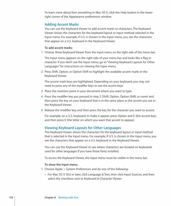
To learn more about font smoothing in Mac OS X, click the Help button in the lower-right corner of the Appearance preferences window.
Adding Accent MarksYou can use the Keyboard Viewer to add accent marks to characters. The Keyboard Viewer shows the characters for the keyboard layout or input method selected in the Input menu. For example, if U.S. is chosen in the Input menu, you see the characters that appear on a U.S. keyboard in the Keyboard Viewer.
To add accent marks:� 1 Choose Show Keyboard Viewer from the Input menu on the right side of the menu bar.
The Input menu appears on the right side of your menu bar and looks like a flag or character. If you don’t see the Input menu, go to “Viewing Keyboard Layouts for Other Languages” for instructions on viewing the Input menu.
2 Press Shift, Option, or Option-Shift to highlight the available accent marks in the Keyboard Viewer.
The accent mark keys are highlighted. Depending on your keyboard, you may not need to press any of the modifier keys to see the accent keys.
3 Place the insertion point in your document where you want to type.
4 Press the modifier key you pressed in step 2 (Shift, Option, Option-Shift, or none) and then press the key on your keyboard that is in the same place as the accent you see in the Keyboard Viewer.
5 Release the modifier key, and then press the key for the character you want to accent.
For example, on a U.S. keyboard, to make é appear, press Option and E (the accent key), and then press E (the letter on which you want that accent to appear).
Viewing Keyboard Layouts for Other LanguagesThe Keyboard Viewer shows the characters for the keyboard layout or input method that is selected in the Input menu. For example, if U.S. is chosen in the Input menu, you see the characters that appear on a U.S. keyboard in the Keyboard Viewer.
You can use the Keyboard Viewer to see where characters are located on keyboards used for other languages if you have those fonts installed.
To access the Keyboard Viewer, the Input menu must be visible in the menu bar.
To show the Input menu:� 1 Choose Apple > System Preferences and do one of the following:
For Mac OS X 10.6 or later, click Language & Text, then click Input Sources, and then Âselect the checkbox next to Keyboard & Character Viewer.
170 Chapter 8 Working with Text
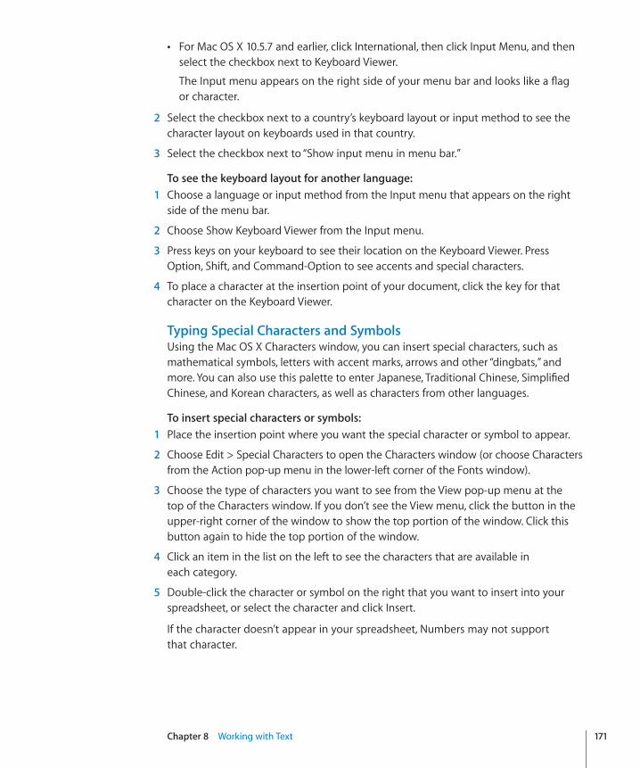
Chapter 8 Working with Text 171
For Mac OS X 10.5.7 and earlier, click International, then click Input Menu, and then Âselect the checkbox next to Keyboard Viewer.
The Input menu appears on the right side of your menu bar and looks like a flag or character.
2 Select the checkbox next to a country’s keyboard layout or input method to see the character layout on keyboards used in that country.
3 Select the checkbox next to “Show input menu in menu bar.”
To see the keyboard layout for another language:� 1 Choose a language or input method from the Input menu that appears on the right
side of the menu bar.
2 Choose Show Keyboard Viewer from the Input menu.
3 Press keys on your keyboard to see their location on the Keyboard Viewer. Press Option, Shift, and Command-Option to see accents and special characters.
4 To place a character at the insertion point of your document, click the key for that character on the Keyboard Viewer.
Typing Special Characters and SymbolsUsing the Mac OS X Characters window, you can insert special characters, such as mathematical symbols, letters with accent marks, arrows and other “dingbats,” and more. You can also use this palette to enter Japanese, Traditional Chinese, Simplified Chinese, and Korean characters, as well as characters from other languages.
To insert special characters or symbols:� 1 Place the insertion point where you want the special character or symbol to appear.
2 Choose Edit > Special Characters to open the Characters window (or choose Characters from the Action pop-up menu in the lower-left corner of the Fonts window).
3 Choose the type of characters you want to see from the View pop-up menu at the top of the Characters window. If you don’t see the View menu, click the button in the upper-right corner of the window to show the top portion of the window. Click this button again to hide the top portion of the window.
4 Click an item in the list on the left to see the characters that are available in each category.
5 Double-click the character or symbol on the right that you want to insert into your spreadsheet, or select the character and click Insert.
If the character doesn’t appear in your spreadsheet, Numbers may not support that character.
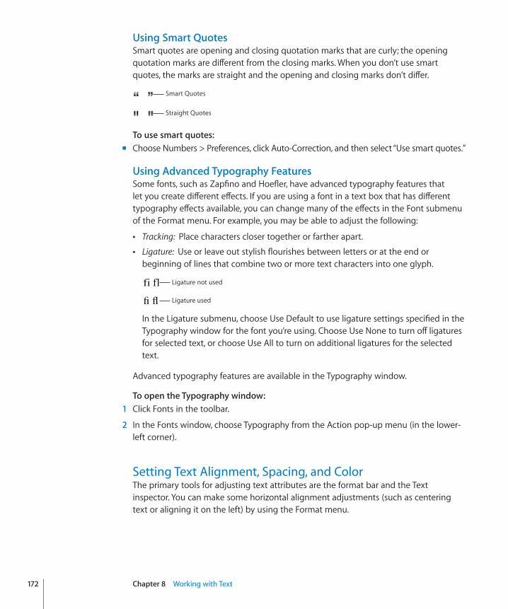
Using Smart QuotesSmart quotes are opening and closing quotation marks that are curly; the opening quotation marks are different from the closing marks. When you don’t use smart quotes, the marks are straight and the opening and closing marks don’t differ.
Smart Quotes
Straight Quotes
To use smart quotes:�Choose Numbers > Preferences, click Auto-Correction, and then select “Use smart quotes.” m
Using Advanced Typography FeaturesSome fonts, such as Zapfino and Hoefler, have advanced typography features that let you create different effects. If you are using a font in a text box that has different typography effects available, you can change many of the effects in the Font submenu of the Format menu. For example, you may be able to adjust the following:
 Tracking: Place characters closer together or farther apart.
 Ligature: Use or leave out stylish flourishes between letters or at the end or beginning of lines that combine two or more text characters into one glyph.
Ligature not used
Ligature used
In the Ligature submenu, choose Use Default to use ligature settings specified in the Typography window for the font you’re using. Choose Use None to turn off ligatures for selected text, or choose Use All to turn on additional ligatures for the selected text.
Advanced typography features are available in the Typography window.
To open the Typography window:� 1 Click Fonts in the toolbar.
2 In the Fonts window, choose Typography from the Action pop-up menu (in the lower-left corner).
Setting Text Alignment, Spacing, and ColorThe primary tools for adjusting text attributes are the format bar and the Text inspector. You can make some horizontal alignment adjustments (such as centering text or aligning it on the left) by using the Format menu.
172 Chapter 8 Working with Text
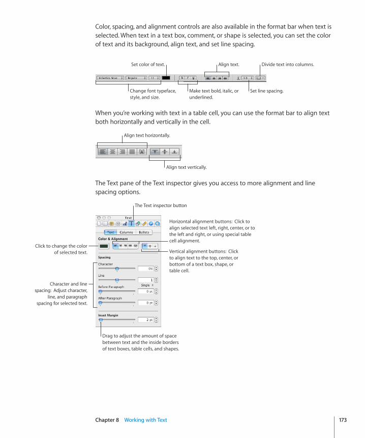
Chapter 8 Working with Text 173
Color, spacing, and alignment controls are also available in the format bar when text is selected. When text in a text box, comment, or shape is selected, you can set the color of text and its background, align text, and set line spacing.
Change font typeface, style, and size.
Set color of text.
Make text bold, italic, or underlined.
Align text.
Set line spacing.
Divide text into columns.
When you’re working with text in a table cell, you can use the format bar to align text both horizontally and vertically in the cell.
Align text vertically.
Align text horizontally.
The Text pane of the Text inspector gives you access to more alignment and line spacing options.
Horizontal alignment buttons: Click to align selected text left, right, center, or to the left and right, or using special table cell alignment.
Vertical alignment buttons: Click to align text to the top, center, or bottom of a text box, shape, or table cell.
Character and line spacing: Adjust character,
line, and paragraph spacing for selected text.
Drag to adjust the amount of space between text and the inside borders of text boxes, table cells, and shapes.
Click to change the color of selected text.
The Text inspector button
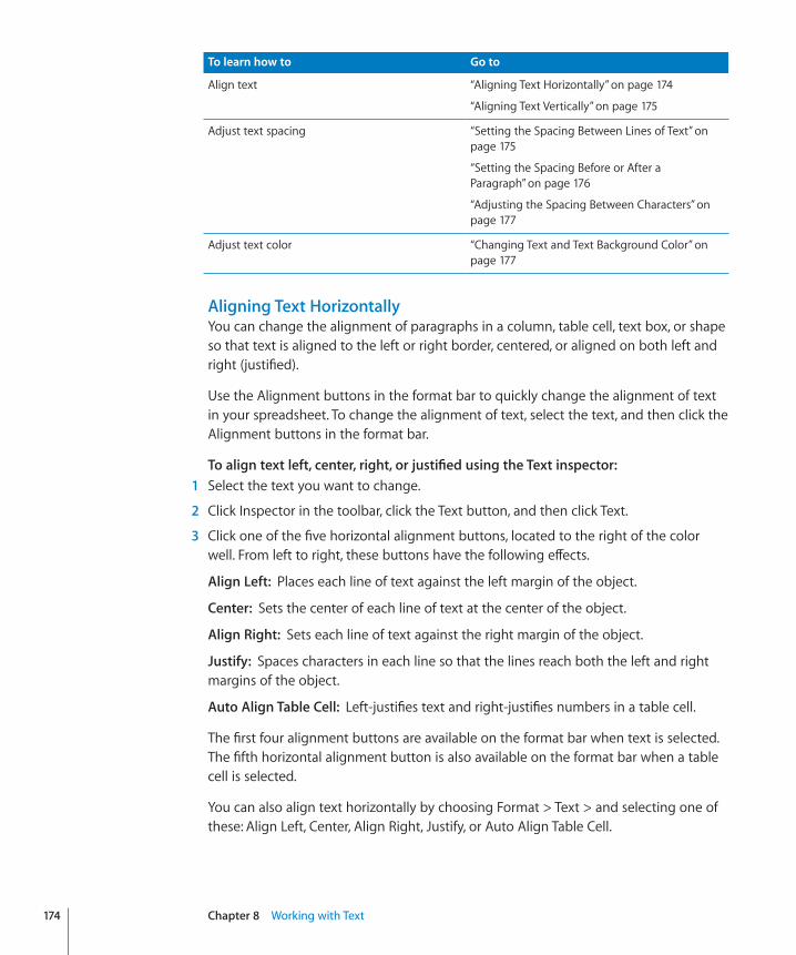
To learn how to Go to
Align text “Aligning Text Horizontally” on page 174
“Aligning Text Vertically” on page 175
Adjust text spacing “Setting the Spacing Between Lines of Text” on page 175
“Setting the Spacing Before or After a Paragraph” on page 176
“Adjusting the Spacing Between Characters” on page 177
Adjust text color “Changing Text and Text Background Color” on page 177
Aligning Text HorizontallyYou can change the alignment of paragraphs in a column, table cell, text box, or shape so that text is aligned to the left or right border, centered, or aligned on both left and right (justified).
Use the Alignment buttons in the format bar to quickly change the alignment of text in your spreadsheet. To change the alignment of text, select the text, and then click the Alignment buttons in the format bar.
To align text left, center, right, or justified using the Text inspector: 1 Select the text you want to change.
2 Click Inspector in the toolbar, click the Text button, and then click Text.
3 Click one of the five horizontal alignment buttons, located to the right of the color well. From left to right, these buttons have the following effects.
Align Left:� Places each line of text against the left margin of the object.
Center:� Sets the center of each line of text at the center of the object.
Align Right:� Sets each line of text against the right margin of the object.
Justify:� Spaces characters in each line so that the lines reach both the left and right margins of the object.
Auto Align Table Cell:� Left-justifies text and right-justifies numbers in a table cell.
The first four alignment buttons are available on the format bar when text is selected. The fifth horizontal alignment button is also available on the format bar when a table cell is selected.
You can also align text horizontally by choosing Format > Text > and selecting one of these: Align Left, Center, Align Right, Justify, or Auto Align Table Cell.
174 Chapter 8 Working with Text
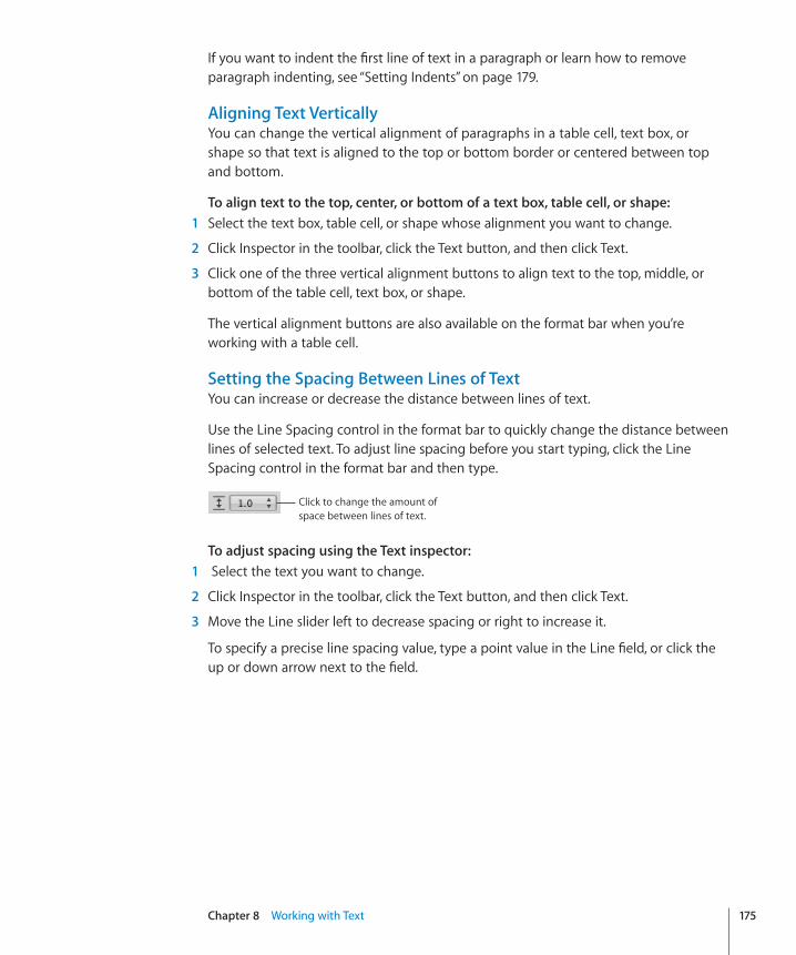
Chapter 8 Working with Text 175
If you want to indent the first line of text in a paragraph or learn how to remove paragraph indenting, see “Setting Indents” on page 179.
Aligning Text VerticallyYou can change the vertical alignment of paragraphs in a table cell, text box, or shape so that text is aligned to the top or bottom border or centered between top and bottom.
To align text to the top, center, or bottom of a text box, table cell, or shape:� 1 Select the text box, table cell, or shape whose alignment you want to change.
2 Click Inspector in the toolbar, click the Text button, and then click Text.
3 Click one of the three vertical alignment buttons to align text to the top, middle, or bottom of the table cell, text box, or shape.
The vertical alignment buttons are also available on the format bar when you’re working with a table cell.
Setting the Spacing Between Lines of TextYou can increase or decrease the distance between lines of text.
Use the Line Spacing control in the format bar to quickly change the distance between lines of selected text. To adjust line spacing before you start typing, click the Line Spacing control in the format bar and then type.
Click to change the amount of space between lines of text.
To adjust spacing using the Text inspector:� 1 Select the text you want to change.
2 Click Inspector in the toolbar, click the Text button, and then click Text.
3 Move the Line slider left to decrease spacing or right to increase it.
To specify a precise line spacing value, type a point value in the Line field, or click the up or down arrow next to the field.
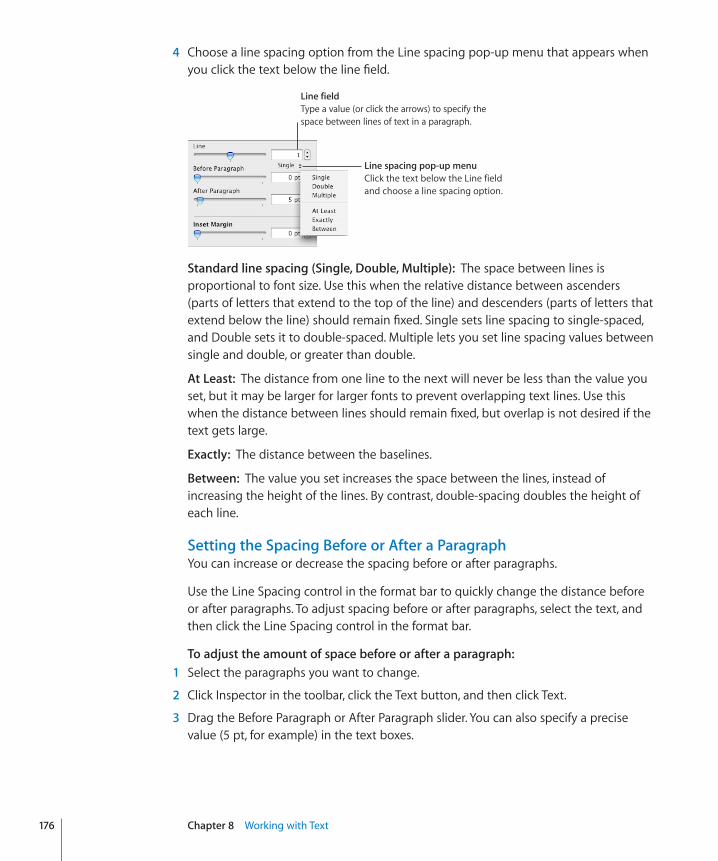
4 Choose a line spacing option from the Line spacing pop-up menu that appears when you click the text below the line field.
Line spacing pop-up menuClick the text below the Line field and choose a line spacing option.
Line fieldType a value (or click the arrows) to specify the space between lines of text in a paragraph.
Standard line spacing (Single, Double, Multiple):� The space between lines is proportional to font size. Use this when the relative distance between ascenders (parts of letters that extend to the top of the line) and descenders (parts of letters that extend below the line) should remain fixed. Single sets line spacing to single-spaced, and Double sets it to double-spaced. Multiple lets you set line spacing values between single and double, or greater than double.
At Least:� The distance from one line to the next will never be less than the value you set, but it may be larger for larger fonts to prevent overlapping text lines. Use this when the distance between lines should remain fixed, but overlap is not desired if the text gets large.
Exactly:� The distance between the baselines.
Between:� The value you set increases the space between the lines, instead of increasing the height of the lines. By contrast, double-spacing doubles the height of each line.
Setting the Spacing Before or After a ParagraphYou can increase or decrease the spacing before or after paragraphs.
Use the Line Spacing control in the format bar to quickly change the distance before or after paragraphs. To adjust spacing before or after paragraphs, select the text, and then click the Line Spacing control in the format bar.
To adjust the amount of space before or after a paragraph:� 1 Select the paragraphs you want to change.
2 Click Inspector in the toolbar, click the Text button, and then click Text.
3 Drag the Before Paragraph or After Paragraph slider. You can also specify a precise value (5 pt, for example) in the text boxes.
176 Chapter 8 Working with Text
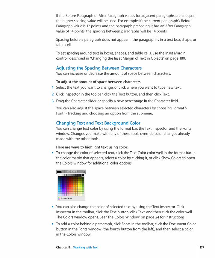
Chapter 8 Working with Text 177
If the Before Paragraph or After Paragraph values for adjacent paragraphs aren’t equal, the higher spacing value will be used. For example, if the current paragraph’s Before Paragraph value is 12 points and the paragraph preceding it has an After Paragraph value of 14 points, the spacing between paragraphs will be 14 points.
Spacing before a paragraph does not appear if the paragraph is in a text box, shape, or table cell.
To set spacing around text in boxes, shapes, and table cells, use the Inset Margin control, described in “Changing the Inset Margin of Text in Objects” on page 180.
Adjusting the Spacing Between CharactersYou can increase or decrease the amount of space between characters.
To adjust the amount of space between characters:� 1 Select the text you want to change, or click where you want to type new text.
2 Click Inspector in the toolbar, click the Text button, and then click Text.
3 Drag the Character slider or specify a new percentage in the Character field.
You can also adjust the space between selected characters by choosing Format > Font > Tracking and choosing an option from the submenu.
Changing Text and Text Background ColorYou can change text color by using the format bar, the Text inspector, and the Fonts window. Changes you make with any of these tools override color changes already made with the other tools.
Here are ways to highlight text using color:�To change the color of selected text, click the Text Color color well in the format bar. In m
the color matrix that appears, select a color by clicking it, or click Show Colors to open the Colors window for additional color options.
You can also change the color of selected text by using the Text inspector. Click m
Inspector in the toolbar, click the Text button, click Text, and then click the color well. The Colors window opens. See “The Colors Window” on page 24 for instructions.
To add a color behind a paragraph, click Fonts in the toolbar, click the Document Color m
button in the Fonts window (the fourth button from the left), and then select a color in the Colors window.
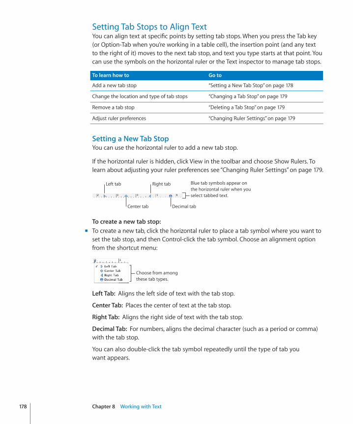
Setting Tab Stops to Align TextYou can align text at specific points by setting tab stops. When you press the Tab key (or Option-Tab when you’re working in a table cell), the insertion point (and any text to the right of it) moves to the next tab stop, and text you type starts at that point. You can use the symbols on the horizontal ruler or the Text inspector to manage tab stops.
To learn how to Go to
Add a new tab stop “Setting a New Tab Stop” on page 178
Change the location and type of tab stops “Changing a Tab Stop” on page 179
Remove a tab stop “Deleting a Tab Stop” on page 179
Adjust ruler preferences “Changing Ruler Settings” on page 179
Setting a New Tab StopYou can use the horizontal ruler to add a new tab stop.
If the horizontal ruler is hidden, click View in the toolbar and choose Show Rulers. To learn about adjusting your ruler preferences see “Changing Ruler Settings” on page 179.
Blue tab symbols appear on the horizontal ruler when you select tabbed text.
Decimal tab
Right tab
Center tab
Left tab
To create a new tab stop:�To create a new tab, click the horizontal ruler to place a tab symbol where you want to m
set the tab stop, and then Control-click the tab symbol. Choose an alignment option from the shortcut menu:
Choose from among these tab types.
Left Tab:� Aligns the left side of text with the tab stop.
Center Tab:� Places the center of text at the tab stop.
Right Tab:� Aligns the right side of text with the tab stop.
Decimal Tab:� For numbers, aligns the decimal character (such as a period or comma) with the tab stop.
You can also double-click the tab symbol repeatedly until the type of tab you want appears.
178 Chapter 8 Working with Text
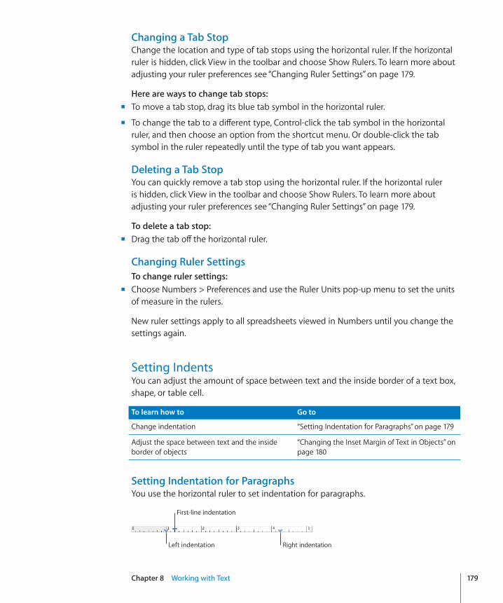
Chapter 8 Working with Text 179
Changing a Tab StopChange the location and type of tab stops using the horizontal ruler. If the horizontal ruler is hidden, click View in the toolbar and choose Show Rulers. To learn more about adjusting your ruler preferences see “Changing Ruler Settings” on page 179.
Here are ways to change tab stops:�To move a tab stop, drag its blue tab symbol in the horizontal ruler. m
To change the tab to a different type, Control-click the tab symbol in the horizontal m
ruler, and then choose an option from the shortcut menu. Or double-click the tab symbol in the ruler repeatedly until the type of tab you want appears.
Deleting a Tab StopYou can quickly remove a tab stop using the horizontal ruler. If the horizontal ruler is hidden, click View in the toolbar and choose Show Rulers. To learn more about adjusting your ruler preferences see “Changing Ruler Settings” on page 179.
To delete a tab stop:�Drag the tab off the horizontal ruler. m
Changing Ruler SettingsTo change ruler settings:�Choose Numbers > Preferences and use the Ruler Units pop-up menu to set the units m
of measure in the rulers.
New ruler settings apply to all spreadsheets viewed in Numbers until you change the settings again.
Setting IndentsYou can adjust the amount of space between text and the inside border of a text box, shape, or table cell.
To learn how to Go to
Change indentation “Setting Indentation for Paragraphs” on page 179
Adjust the space between text and the inside border of objects
“Changing the Inset Margin of Text in Objects” on page 180
Setting Indentation for ParagraphsYou use the horizontal ruler to set indentation for paragraphs.
First-line indentation
Left indentation Right indentation
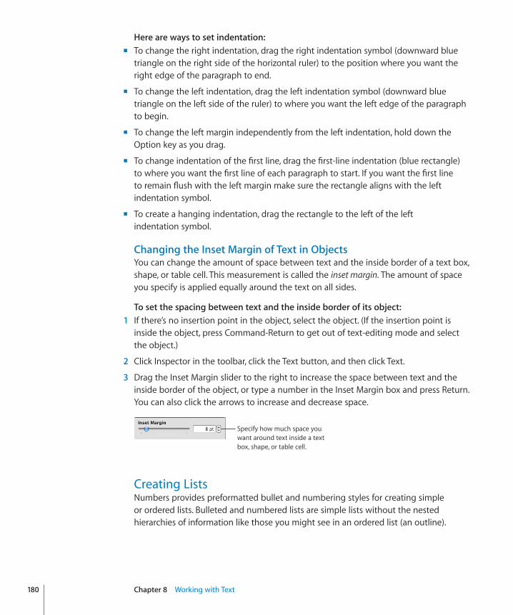
Here are ways to set indentation:�To change the right indentation, drag the right indentation symbol (downward blue m
triangle on the right side of the horizontal ruler) to the position where you want the right edge of the paragraph to end.
To change the left indentation, drag the left indentation symbol (downward blue m
triangle on the left side of the ruler) to where you want the left edge of the paragraph to begin.
To change the left margin independently from the left indentation, hold down the m
Option key as you drag.
To change indentation of the first line, drag the first-line indentation (blue rectangle) m
to where you want the first line of each paragraph to start. If you want the first line to remain flush with the left margin make sure the rectangle aligns with the left indentation symbol.
To create a hanging indentation, drag the rectangle to the left of the left m
indentation symbol.
Changing the Inset Margin of Text in ObjectsYou can change the amount of space between text and the inside border of a text box, shape, or table cell. This measurement is called the inset margin. The amount of space you specify is applied equally around the text on all sides.
To set the spacing between text and the inside border of its object:� 1 If there’s no insertion point in the object, select the object. (If the insertion point is
inside the object, press Command-Return to get out of text-editing mode and select the object.)
2 Click Inspector in the toolbar, click the Text button, and then click Text.
3 Drag the Inset Margin slider to the right to increase the space between text and the inside border of the object, or type a number in the Inset Margin box and press Return. You can also click the arrows to increase and decrease space.
Specify how much space you want around text inside a text box, shape, or table cell.
Creating ListsNumbers provides preformatted bullet and numbering styles for creating simple or ordered lists. Bulleted and numbered lists are simple lists without the nested hierarchies of information like those you might see in an ordered list (an outline).
180 Chapter 8 Working with Text
Chapter 8 Working with Text 181
To learn how to Go to
Create lists automatically based on what you type “Generating Lists Automatically” on page 181
Use the Text inspector to format bulleted lists “Formatting Bulleted Lists” on page 181
Use the Text inspector to format numbered lists “Formatting Numbered Lists” on page 182
Use the Text inspector to add and format ordered lists (outlines)
“Formatting Ordered Lists” on page 183
Generating Lists AutomaticallyWhen you use automatic list generation, Numbers automatically formats a list for you based on what you type. To use this feature, first choose Numbers > Preferences, click Auto-Correction, and make sure that “Automatically detect lists” is selected.
To create a list automatically:� 1 Place the insertion point where you want the list to begin.
2 Create a list by doing one of the following:
To create a bulleted list, press Option-8 to type a bullet (•), type an asterisk (*), or Âtype a hyphen (-). Then type a space followed by some text, and press Return. To learn how to format your bulleted list see “Formatting Bulleted Lists” on page 181.
To create a list with labels that are numbers, letters, or Roman numerals, type the Ânumber, letter, or Roman numeral; a period; a space; and then some text. Then press Return. To learn how to format your numbered or ordered list see “Formatting Numbered Lists” on page 182 and “Formatting Ordered Lists” on page 183.
3 Continue to build your list by doing any of the following:
To add a new topic at the current indent level, press Return. Â
To move a list topic at the next lower indent level, press Tab. To move a list topic at Âthe next higher level, press Shift-Tab.
4 To end your list, press Return twice, or press Return and then press Delete.
Note: If you’re working in a table cell and “Return key moves to next cell” is selected in the Table inspector, press Option-Return instead of Return.
Formatting Bulleted ListsAlthough you can use automatic list generation to create a simple bulleted list, using the Text inspector gives you many options for formatting bulleted lists. See “Generating Lists Automatically” on page 181 for information about creating a list automatically.
To add and format a bulleted list using the Text inspector:� 1 Place the insertion point where you want the list to begin.
2 Click Inspector in the toolbar, click the Text inspector button, and then click Bullets.
3 Choose a bullet style from the Bullets & Numbering pop-up menu.
To use a typed character as a bullet, choose Text Bullets and choose a character from the list or type a new character in the field.
To use one of the image bullets that comes with Numbers, choose Image Bullets, and then choose an image from the scrolling list.
To use your own image as a bullet, choose Custom Image, and then choose an image in the Open dialog that appears.
4 To change the size of an image bullet, specify a percentage of the original image size in the Size field. Or, select the “Scale with text” checkbox and specify a percentage of the text size; this option maintains the image-to-text size ratio of the bullets even if you later change the font size of text.
5 To adjust the space between bullets and the left margin, use the Bullet Indent field. To adjust the space between bullets and text, use the Text Indent field.
6 To position bullets higher or lower relative to text in a text box or shape, use the Align field.
7 To add and indent bulleted items in your list, do any of the following:
To add a new topic at the current indent level, press Return. If you’re working in a Âtable cell and “Return key moves to next cell” is selected in the Table inspector, press Option-Return instead.
To create an unbulleted paragraph within a topic, press Return while holding down Âthe Shift key. If you’re working in a table cell and “Return key moves to next cell” is selected in the Table inspector, press Control-Return instead.
To enter a new topic at the next lower indent level, press Tab. To enter a new topic Âat the next higher level, press Shift-Tab. You can also click and hold a bullet, and then drag to the right, to the left, down and to the right, or down and to the left.
If you’re working in a table cell and “Return key moves to next cell” is selected in the Table inspector, use the Indent Level controls in the Bullets pane of the Text inspector to change the level of entries.
To return to regular text at the end of your list, press Return and choose No Bullets Âfrom the Bullets & Numbering pop-up menu. You may also need to adjust the indent level.
If you’re working in a table cell and “Return key moves to next cell” is selected in the Table inspector, press Option-Return instead of Return.
Formatting Numbered ListsAlthough you can use automatic list generation to create a simple numbered list, using the Text inspector gives you many options for formatting numbered lists. See “Generating Lists Automatically” on page 181 for information about creating a list automatically.
182 Chapter 8 Working with Text
Chapter 8 Working with Text 183
To add and format a numbered list:� 1 Place the insertion point where you want the list to begin.
2 Click Inspector in the toolbar, click the Text inspector button, and then click Bullets.
3 Choose Numbers from the Bullets & Numbering pop-up menu, and then choose a numbering style from the pop-up menu directly below it.
4 To adjust the space between numbers and the left margin, use the Number Indent field. To adjust the space between numbers and text, use the Text Indent field.
5 To add and indent items in your list, do any of the following:
To add a new topic at the current indent level, press Return. If you’re working in a Âtable cell and “Return key moves to next cell” is selected in the Table inspector, press Option-Return instead.
To create an unnumbered paragraph within a topic, press Return while holding Âdown the Shift key. If you’re working in a table cell and “Return key moves to next cell” is selected in the Table inspector, press Control-Return instead.
To enter a new topic at the next lower indent level, press Tab. To enter a new topic Âat the next higher level, press Shift-Tab. You can also click and hold a number, and then drag to the right, to the left, down and to the right, or down and to the left.
If you’re working in a table cell and “Return key moves to next cell” is selected in the Table inspector, use the Indent Level controls in the Bullets pane of the Text inspector to change the level of entries.
To return to regular text at the end of your list, press Return and choose No Bullets Âfrom the Bullets & Numbering pop-up menu. You may also need to adjust the indent level.
If you’re working in a table cell and “Return key moves to next cell” is selected in the Table inspector, press Option-Return instead of Return.
To add an existing paragraph to a numbered list, click the paragraph, choose a Ânumbering style, and click “Continue from previous.”
To start a new numbered sequence in a list, click “Start at” and specify the number Âyou want the sequence to begin with.
If you want items in your list to have labeled subtopics (as in an outline), use an ordered list instead of a numbered list.
Formatting Ordered ListsOrdered lists provide different numbering styles for each indent level in a list, allowing you to create a hierarchy of information. For example:
You can create a list using a numbering sequence as you proceed from the highest Âlevel to lower levels: I, A, 1, a), (1), (a), i), (1), and (a).
You can create a legal list style, which appends an additional number or letter at Âeach lower level: 1, 1.1, 1.1.1, and so on.
To add and format an ordered list:� 1 Place the insertion point where you want the list to begin.
2 Click Inspector in the toolbar, click the Text inspector button, and then click Bullets.
3 To create a legal style list, choose Tiered Numbers from the Bullets & Numbering pop-up menu. Otherwise, choose Numbers instead.
4 Choose a numbering style from the pop-up menu directly below it.
5 To adjust the space between numbers and the left margin, use the Number Indent field. To adjust the space between numbers and text, use the Text Indent field.
6 To add and indent items in your list, do any of the following:
To add a new topic at the current indent level, press Return. If you’re working in a Âtable cell and “Return key moves to next cell” is selected in the Table inspector, press Option-Return instead.
To create an unnumbered paragraph within a topic, press Return while holding Âdown the Shift key. If you’re working in a table cell and “Return key moves to next cell” is selected in the Table inspector, press Control-Return instead.
To enter a new topic at the next lower indent level, press Tab. To enter a new topic Âat the next higher level, press Shift-Tab. To move among levels you can also click and hold a number, and then drag to the right, to the left, down and to the right, or down and to the left.
If you’re working in a table cell and “Return key moves to next cell” is selected in the Table inspector, use the Indent Level controls in the Bullets pane of the Text inspector to change the level of entries.
To return to regular text at the end of your list, press Return and choose No Bullets Âfrom the Bullets & Numbering pop-up menu. You may also need to adjust the indent level.
If you’re working in a table cell and “Return key moves to next cell” is selected in the Table inspector, press Option-Return instead of Return.
To add an existing paragraph to a numbered list, click the paragraph, choose a Ânumbering style, and then click “Continue from previous.”
To start a new numbered sequence in a list, click “Start at” and specify the number Âyou want the sequence to begin with.
184 Chapter 8 Working with Text
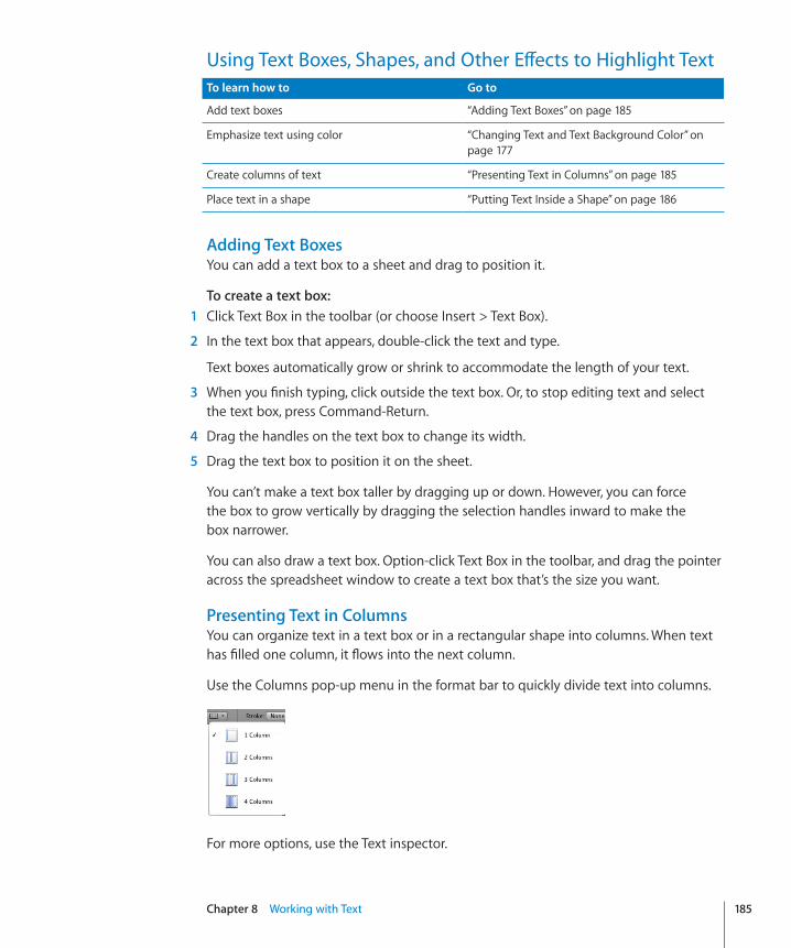
Chapter 8 Working with Text 185
Using Text Boxes, Shapes, and Other Effects to Highlight TextTo learn how to Go to
Add text boxes “Adding Text Boxes” on page 185
Emphasize text using color “Changing Text and Text Background Color” on page 177
Create columns of text “Presenting Text in Columns” on page 185
Place text in a shape “Putting Text Inside a Shape” on page 186
Adding Text BoxesYou can add a text box to a sheet and drag to position it.
To create a text box:� 1 Click Text Box in the toolbar (or choose Insert > Text Box).
2 In the text box that appears, double-click the text and type.
Text boxes automatically grow or shrink to accommodate the length of your text.
3 When you finish typing, click outside the text box. Or, to stop editing text and select the text box, press Command-Return.
4 Drag the handles on the text box to change its width.
5 Drag the text box to position it on the sheet.
You can’t make a text box taller by dragging up or down. However, you can force the box to grow vertically by dragging the selection handles inward to make the box narrower.
You can also draw a text box. Option-click Text Box in the toolbar, and drag the pointer across the spreadsheet window to create a text box that’s the size you want.
Presenting Text in ColumnsYou can organize text in a text box or in a rectangular shape into columns. When text has filled one column, it flows into the next column.
Use the Columns pop-up menu in the format bar to quickly divide text into columns.
For more options, use the Text inspector.
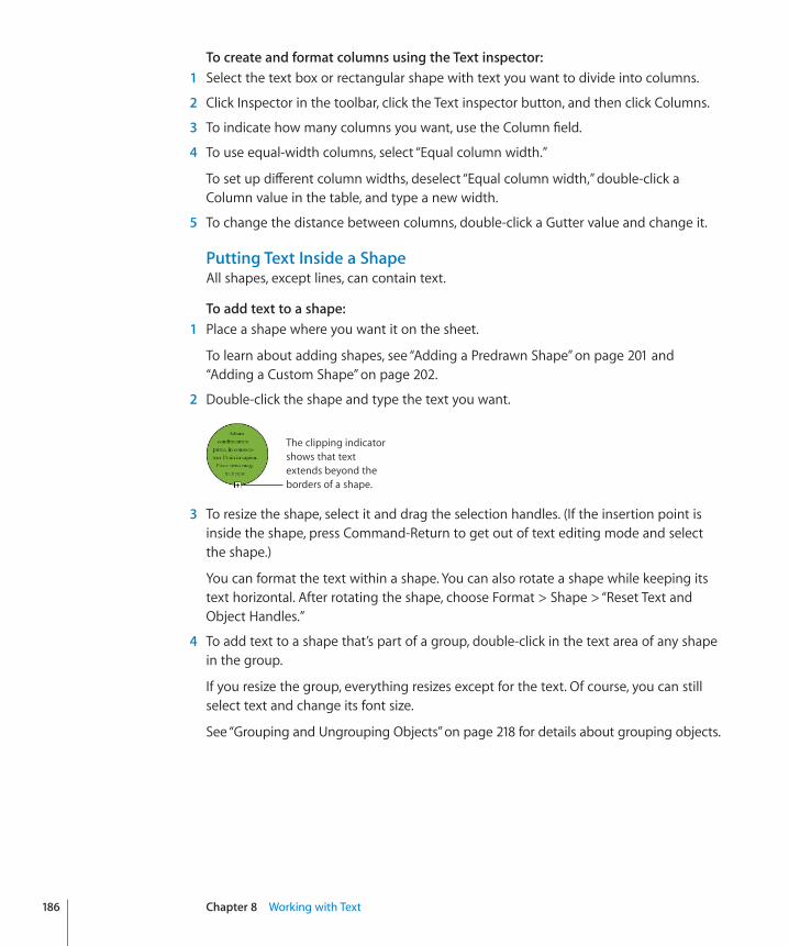
To create and format columns using the Text inspector:� 1 Select the text box or rectangular shape with text you want to divide into columns.
2 Click Inspector in the toolbar, click the Text inspector button, and then click Columns.
3 To indicate how many columns you want, use the Column field.
4 To use equal-width columns, select “Equal column width.”
To set up different column widths, deselect “Equal column width,” double-click a Column value in the table, and type a new width.
5 To change the distance between columns, double-click a Gutter value and change it.
Putting Text Inside a ShapeAll shapes, except lines, can contain text.
To add text to a shape:� 1 Place a shape where you want it on the sheet.
To learn about adding shapes, see “Adding a Predrawn Shape” on page 201 and “Adding a Custom Shape” on page 202.
2 Double-click the shape and type the text you want.
The clipping indicator shows that text extends beyond the borders of a shape.
3 To resize the shape, select it and drag the selection handles. (If the insertion point is inside the shape, press Command-Return to get out of text editing mode and select the shape.)
You can format the text within a shape. You can also rotate a shape while keeping its text horizontal. After rotating the shape, choose Format > Shape > “Reset Text and Object Handles.”
4 To add text to a shape that’s part of a group, double-click in the text area of any shape in the group.
If you resize the group, everything resizes except for the text. Of course, you can still select text and change its font size.
See “Grouping and Ungrouping Objects” on page 218 for details about grouping objects.
186 Chapter 8 Working with Text
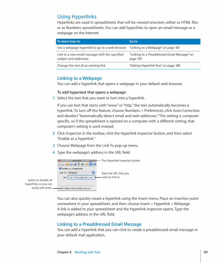
Chapter 8 Working with Text 187
Using HyperlinksHyperlinks are used in spreadsheets that will be viewed onscreen, either as HTML files or as Numbers spreadsheets. You can add hyperlinks to open an email message or a webpage on the Internet.
To learn how to Go to
Use a webpage hyperlink to go to a web browser “Linking to a Webpage” on page 187
Link to a new email message with the specified subject and addressee
“Linking to a Preaddressed Email Message” on page 187
Change the text of an existing link “Editing Hyperlink Text” on page 188
Linking to a WebpageYou can add a hyperlink that opens a webpage in your default web browser.
To add hypertext that opens a webpage:� 1 Select the text that you want to turn into a hyperlink.
If you use text that starts with “www” or “http,” the text automatically becomes a hyperlink. To turn off this feature, choose Numbers > Preferences, click Auto-Correction, and deselect “Automatically detect email and web addresses.” This setting is computer specific, so if the spreadsheet is opened on a computer with a different setting, that computer’s setting is used instead.
2 Click Inspector in the toolbar, click the Hyperlink inspector button, and then select “Enable as a hyperlink.”
3 Choose Webpage from the Link To pop-up menu.
4 Type the webpage’s address in the URL field.
The Hyperlink inspector button
Type the URL that you want to link to.
Select to disable all hyperlinks so you can
easily edit them.
You can also quickly create a hyperlink using the Insert menu. Place an insertion point somewhere in your spreadsheet, and then choose Insert > Hyperlink > Webpage. A link is added to your spreadsheet and the Hyperlink inspector opens. Type the webpage’s address in the URL field.
Linking to a Preaddressed Email MessageYou can add a hyperlink that you can click to create a preaddressed email message in your default mail application.
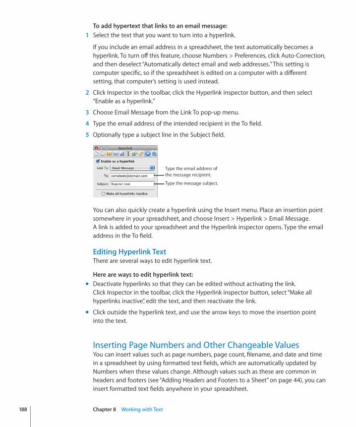
To add hypertext that links to an email message:� 1 Select the text that you want to turn into a hyperlink.
If you include an email address in a spreadsheet, the text automatically becomes a hyperlink. To turn off this feature, choose Numbers > Preferences, click Auto-Correction, and then deselect “Automatically detect email and web addresses.” This setting is computer specific, so if the spreadsheet is edited on a computer with a different setting, that computer’s setting is used instead.
2 Click Inspector in the toolbar, click the Hyperlink inspector button, and then select “Enable as a hyperlink.”
3 Choose Email Message from the Link To pop-up menu.
4 Type the email address of the intended recipient in the To field.
5 Optionally type a subject line in the Subject field.
Type the email address of the message recipient.
Type the message subject.
You can also quickly create a hyperlink using the Insert menu. Place an insertion point somewhere in your spreadsheet, and choose Insert > Hyperlink > Email Message. A link is added to your spreadsheet and the Hyperlink inspector opens. Type the email address in the To field.
Editing Hyperlink TextThere are several ways to edit hyperlink text.
Here are ways to edit hyperlink text:�Deactivate hyperlinks so that they can be edited without activating the link. m
Click Inspector in the toolbar, click the Hyperlink inspector button, select “Make all hyperlinks inactive”, edit the text, and then reactivate the link.
Click outside the hyperlink text, and use the arrow keys to move the insertion point m
into the text.
Inserting Page Numbers and Other Changeable ValuesYou can insert values such as page numbers, page count, filename, and date and time in a spreadsheet by using formatted text fields, which are automatically updated by Numbers when these values change. Although values such as these are common in headers and footers (see “Adding Headers and Footers to a Sheet” on page 44), you can insert formatted text fields anywhere in your spreadsheet.
188 Chapter 8 Working with Text
Chapter 8 Working with Text 189
Here are ways to insert formatted text fields:To add page numbers, place the insertion point where you want the page number to m
appear, and then choose Insert > Page Number.
To change the page number format, Control-click a page number and choose a new number format.
To add the total page count, place the insertion point where you want the page count m
to appear, and then choose Insert > Page Count.
To include the total page count with each page number, such as “2 of 10,” add a page number, type “of,” and then choose Insert > Page Count.
To change the page count format, Control-click a page count and choose a new number format.
To add and format the date and time, place the insertion point where you want the m
value to appear, and then choose Insert > Date & Time.
To change the date and time format, Control-click the date and time value, choose Edit Date & Time, and then choose a date and time format from the pop-up menu. If you want the spreadsheet to always show the current date and time, select “Automatically update on open.”
To add the spreadsheet’s filename, place the insertion point where you want the m
filename to appear, and then choose Insert > Filename.
To display the file directory path, double-click the filename and select “Show directory path.”
To display the file extension, double-click the filename and select “Always show filename extension.”
Automatically Substituting TextNumbers can be set to recognize and replace text you don’t want with text you do want. For example, when you type “teh,” Numbers can automatically change it to “the.”
To set up automatic text substitution:� 1 Choose Numbers > Preferences.
2 Click Auto-Correction and specify settings as desired.
To automatically convert single and double quotation marks to smart quotes so that opening and closing quotation marks are not identical, select “Use smart quotes.”
To make sure that the first word in a sentence begins with a capital letter, select “Fix capitalization.”
To automatically convert the letters in “1st,” “2nd,” “3rd,” and so on into superscripts, select “Superscript numerical suffixes.”
To set Numbers to automatically detect that something you’ve typed is an email address or a URL, select “Automatically detect email and web addresses.” Email and web addresses you type automatically become hyperlinks for Mail or Safari.
To use automatic list generation, select “Automatically detect lists.”
To automatically replace misspelled words if there is only one option in the spelling dictionary, select “Automatically use spell checker suggestions.”
To replace one or more characters with one or more different characters, select “Symbol and text substitution.” Then use the rows in the table to define and activate specific substitutions. For example, when you type (c), you can have Numbers automatically convert it to © by putting a checkmark in the On column. To add a row to the table to define your own substitution, click the Add (+) button. To remove a selected item, click the Delete (–) button.
After you specify substitution settings, they’ll apply to any text you change or add in any Numbers spreadsheet.
Inserting a Nonbreaking SpaceYou can insert a nonbreaking space between words to make sure that the words always appear in the same line of text.
To insert a nonbreaking space:�Press the Space bar while holding down the Option key. m
Checking for Misspelled WordsYou can set the spell checker to flag spelling errors as you type, or you can check your entire spreadsheet or selected text at any time.
Misspelled words appear with a red dashed line below them.
Here are ways to find misspelled words:To check spelling as you type, choose Edit > Spelling > “Check Spelling as You Type.” m
To turn off spell checking as you type, click Edit > Spelling > “Check Spelling as You Type” to deselect it (make sure the checkmark is not visible next to the command).
To check spelling from the insertion point to the end of the spreadsheet, click to place m
the insertion point and choose Edit > Spelling > Check Spelling. To limit spell checking to a specific part of the spreadsheet, select the text you want to check before choosing the command.
The first misspelled word found is highlighted. You can correct it or choose the same command again to continue checking the spreadsheet.
190 Chapter 8 Working with Text
Chapter 8 Working with Text 191
To go through the text more quickly, press Command-semicolon (;) to continue checking the spreadsheet.
To check spelling m and view suggestions for misspelled words, choose Edit > Spelling > Spelling.
The Spelling window opens, and you can use it as “Working with Spelling Suggestions” on page 191 describes.
To automatically accept the spelling suggestions, choose Pages > Preferences, click Auto-Correction, and then select “Automatically use spell checker suggestions”.
Working with Spelling SuggestionsUse the Spelling window to work with alternative spellings.
To work with spelling suggestions:� 1 Choose Edit > Spelling > Spelling.
The Spelling window opens and the first misspelled word is highlighted.
2 Each language has a different spelling dictionary. To make sure that the correct language is selected, select the text you want to work with, click Inspector in the toolbar, click the Text button, and then click More. Select a language from the Language pop-up menu.
3 To replace the incorrect spelling in the text, double-click the correct word or spelling in the list of suggested corrections.
4 If the correct word doesn’t appear in the list of suggested corrections but you know the correct spelling, select the misspelled word in the Spelling window, type the correct word, and click Correct.
5 If the current spelling is correct and you want to leave it as it is, click Ignore or Learn. Use Learn if the term is one you use often and you want to add it to the spelling dictionary.
If you used Learn and want to undo the effect of the Learn operation, do one of the following:
On Mac OS X version 10.4, type the word into the text field below the list of Âsuggested corrections, and then click Forget.
On Mac OS X version 10.5, Control-click the word and choose Unlearn Spelling from Âthe pop-up menu.
6 If no alternative spellings appear in the list of suggested corrections on Mac OS X version 10.4, select the misspelled word in the Spelling window and try a different spelling. Click Guess to see whether new possibilities appear in the list of suggested corrections.
7 Click Find Next and repeat steps 2 through 6 until you find no more spelling errors.
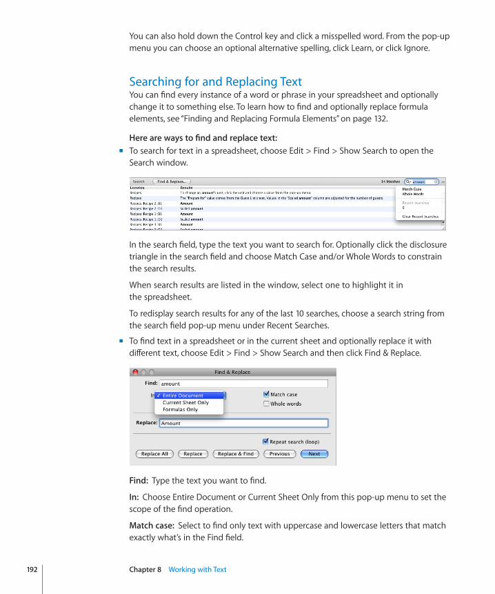
You can also hold down the Control key and click a misspelled word. From the pop-up menu you can choose an optional alternative spelling, click Learn, or click Ignore.
Searching for and Replacing TextYou can find every instance of a word or phrase in your spreadsheet and optionally change it to something else. To learn how to find and optionally replace formula elements, see “Finding and Replacing Formula Elements” on page 132.
Here are ways to find and replace text:To search for text in a spreadsheet, choose Edit > Find > Show Search to open the m
Search window.
In the search field, type the text you want to search for. Optionally click the disclosure triangle in the search field and choose Match Case and/or Whole Words to constrain the search results.
When search results are listed in the window, select one to highlight it in the spreadsheet.
To redisplay search results for any of the last 10 searches, choose a search string from the search field pop-up menu under Recent Searches.
To find text in a spreadsheet or in the current sheet and optionally replace it with m
different text, choose Edit > Find > Show Search and then click Find & Replace.
Find:� Type the text you want to find.
In:� Choose Entire Document or Current Sheet Only from this pop-up menu to set the scope of the find operation.
Match case:� Select to find only text with uppercase and lowercase letters that match exactly what’s in the Find field.
192 Chapter 8 Working with Text

Chapter 8 Working with Text 193
Whole words:� Select to find only text that matches what’s in the Find field in its entirety.
Replace:� Type replacement text in this field.
Repeat search (loop):� Select to continue looking for what’s in the Find field even after the entire spreadsheet or sheet has been searched.
Next or Previous:� Click to search for the next or previous instance of what’s in the Find field. When an element is found, the Formula Editor opens and displays the formula containing the instance of the element.
Replace All:� Click to replace all instances of what’s in the Find field with what’s in the Replace field.
Replace:� Click to replace the current instance of what’s in the Find field with what’s in the Replace field.
Replace & Find:� Click to replace the current instance of what’s in the Find field and to locate the next instance.
Use the other commands on the Edit > Find submenu for additional operations. m
Find Next or Find Previous:� Finds the next or previous occurrence of the current Find text without replacing it, starting with the current sheet or selected cell(s) and proceeding forward or backward through the spreadsheet.
Use selection for Find:� Finds the next occurrence of the selected text.
Jump to Selection:� Displays the selected text when it’s not currently in view.
194
Learn how to add images, shapes, sound, and movies to your spreadsheets.
An object is any item you add to a spreadsheet and then manipulate. Images, shapes, movies, text boxes, tables, and charts are all objects.
This chapter focuses on images (photographs or PDF files), shapes, sound, and movies. Many of the techniques covered in this chapter for placing and manipulating these objects can be generalized to tables, charts, and text boxes; any special formatting techniques for these objects are covered in other chapters.
Working with ImagesNumbers accepts all QuickTime-supported formats, including the following graphics file types:
TIFF Â
GIF Â
JPEG Â
PDF Â
PSD Â
EPS Â
PICT Â
If you intend to greatly enlarge or reduce an image’s dimensions, consider converting it to a PDF file before importing it. PDF files don’t lose their crispness when they’re significantly resized; other file types may not retain their clarity as well when they’re resized. You can convert an image to a PDF by using Grab. Open Grab (it’s in the Applications/Utilities folder), choose Capture > Selection to capture an image, and then choose File > Print to save the image as a PDF.
To import an image, do any of the following:�Choose Insert > Choose, select the file, and then click Insert. m
9Working with Shapes, Graphics, and Other Objects
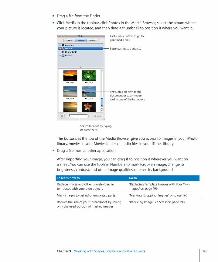
Chapter 9 Working with Shapes, Graphics, and Other Objects 195
Drag a file from the Finder. m
Click Media in the toolbar, click Photos in the Media Browser, select the album where m
your picture is located, and then drag a thumbnail to position it where you want it.
Second, choose a source.
First, click a button to go to your media files.
Third, drag an item to the document or to an image well in one of the inspectors.
Search for a file by typing its name here.
The buttons at the top of the Media Browser give you access to images in your iPhoto library, movies in your Movies folder, or audio files in your iTunes library.
Drag a file from another application. m
After importing your image, you can drag it to position it wherever you want on a sheet. You can use the tools in Numbers to mask (crop) an image; change its brightness, contrast, and other image qualities; or erase its background.
To learn how to Go to
Replace image and other placeholders in templates with your own objects
“Replacing Template Images with Your Own Images” on page 196
Mask images to get rid of unwanted parts “Masking (Cropping) Images” on page 196
Reduce the size of your spreadsheet by saving only the used portion of masked images
“Reducing Image File Sizes” on page 198
To learn how to Go to
Make parts of an image transparent in order to remove the image background
“Removing the Background or Unwanted Elements from an Image” on page 198
Improve the quality of images and create interesting visual effects
“Changing an Image’s Brightness, Contrast, and Other Settings” on page 199
Place, align, resize, and reformat images “Manipulating, Arranging, and Changing the Look of Objects” on page 212
Add an equation you can manipulate like an image
“Working with MathType” on page 230
Replacing Template Images with Your Own ImagesThe photos you see featured in Numbers templates are actually media placeholders. By dragging your own images to these placeholders, your media is automatically sized, positioned, and framed to fit the template.
To test whether an image is a placeholder, let the pointer rest over it and see if a help tag appears instructing you to drag your own file to the placeholder.
Here are ways to work with media placeholders:�To replace a media placeholder with your own image, drag it from the Media Browser, m
the Finder, or another application to the placeholder.
To resize or reposition your image within a media placeholder, click the Edit Mask m
button that hovers over the image after you drop it onto the placeholder, and then do any of the following:
To resize your image within the placeholder, drag the resize handle above the Edit Mask button.
To reposition your image within the placeholder, position the pointer over the image (the pointer may appear as a hand), and then drag the image to position it where you want.
To replace an item you’ve already placed in a media placeholder, drag a new file to it. You don’t have to delete the old file first.
To reposition a media placeholder on a sheet, drag it. m
To remove a media placeholder from a sheet, select it and press Delete. m
Masking (Cropping) ImagesYou can crop images without actually changing the image files by masking the edges to get rid of unwanted parts or to change the outline of the image. If you don’t specify a shape for the mask, by default Numbers uses a rectangular mask. However, you can use any shape available in Numbers, including a custom shape that you’ve created with the Draw tool, to mask the edges of your image.
196 Chapter 9 Working with Shapes, Graphics, and Other Objects
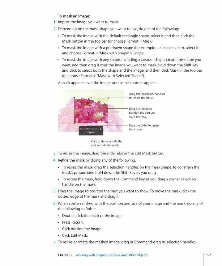
Chapter 9 Working with Shapes, Graphics, and Other Objects 197
To mask an image:� 1 Import the image you want to mask.
2 Depending on the mask shape you want to use, do one of the following:
To mask the image with the default rectangle shape, select it and then click the ÂMask button in the toolbar (or choose Format > Mask).
To mask the image with a predrawn shape (for example, a circle or a star), select it Âand choose Format > “Mask with Shape” > Shape.
To mask the image with any shape, including a custom shape, create the shape you Âwant, and then drag it over the image you want to mask. Hold down the Shift key and click to select both the shape and the image, and then click Mask in the toolbar (or choose Format > “Mask with Selected Shape”).
A mask appears over the image, and some controls appear.
Drag the image to position the part you want to show.
Drag the slider to resize the image.
Click to show or hide the area outside the mask.
Drag the selection handles to resize the mask.
3 To resize the image, drag the slider above the Edit Mask button.
4 Refine the mask by doing any of the following:
To resize the mask, drag the selection handles on the mask shape. To constrain the Âmask’s proportions, hold down the Shift key as you drag.
To rotate the mask, hold down the Command key as you drag a corner selection Âhandle on the mask.
5 Drag the image to position the part you want to show. To move the mask, click the dotted edge of the mask and drag it.
6 When you’re satisfied with the position and size of your image and the mask, do any of the following to finish:
Double-click the mask or the image. Â
Press Return. Â
Click outside the image. Â
Click Edit Mask. Â
7 To resize or rotate the masked image, drag or Command-drag its selection handles.
8 To change the size or position of the mask or the image within it, select the masked image, and then click Edit Mask.
Repeat the steps above as needed.
9 To unmask the image, click Unmask in the toolbar (or choose Format > Unmask).
If you mask a very large image file and you need to use only the smaller version in your spreadsheet, you can have Numbers keep only the smaller copy of the image, thus reducing the overall size of your spreadsheet. See “Reducing Image File Sizes” on page 198.
Reducing Image File SizesIf you resized or masked a very large image file, and you want to save the image file as part of your Numbers spreadsheet (so that you can easily transfer it to another computer), but you want to keep the document size to a minimum, you can choose to save only the smaller (cropped or shrunk) version of the image in your spreadsheet.
Before you reduce the image file size, you must save your document. For details about how to do this, see “Saving a Spreadsheet” on page 32.
Here are ways to reduce the size of images:�To reduce the file size of an individual image that you masked or resized to a smaller m
size, select the image and choose Format > Image > Reduce Image File Size.
To reduce the file size of all masked and resized (shrunk) images, deselect all elements m
on the sheet, and then choose File > Reduce File Size.
Important: After you reduce the size of masked or shrunk image files, you won’t be able to restore them to their original size. If you later want to restore their original size, you must add the original image files to the document again.
Images used in image fills can’t be reduced in this way. Some types of image files also may not be reducible.
To learn about reducing the size of audio and movie files, see “Reducing the Size of Media Files” on page 212.
Removing the Background or Unwanted Elements from an ImageThe Instant Alpha tool lets you to make parts of an image transparent in order to remove the image background.
You get the best results removing solid colors with clear boundaries around them. To remove areas that are less distinct, select a smaller area and repeat the process.
To remove unwanted elements:� 1 Select the image.
2 Choose Format > Instant Alpha.
198 Chapter 9 Working with Shapes, Graphics, and Other Objects
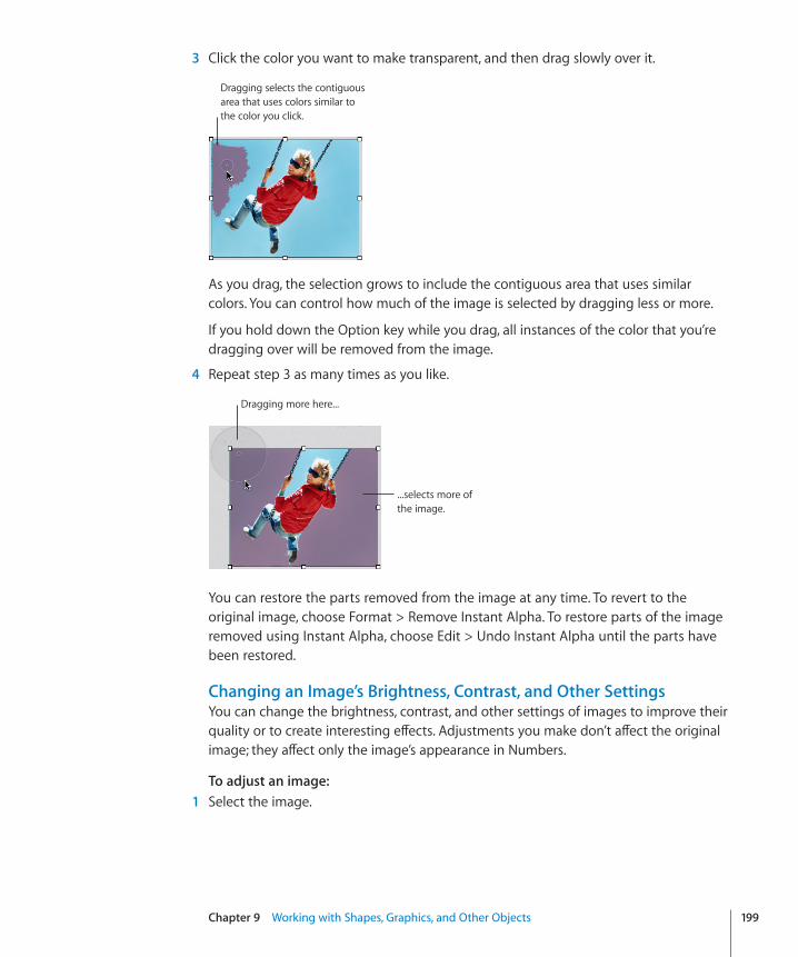
Chapter 9 Working with Shapes, Graphics, and Other Objects 199
3 Click the color you want to make transparent, and then drag slowly over it.
Dragging selects the contiguous area that uses colors similar to the color you click.
As you drag, the selection grows to include the contiguous area that uses similar colors. You can control how much of the image is selected by dragging less or more.
If you hold down the Option key while you drag, all instances of the color that you’re dragging over will be removed from the image.
4 Repeat step 3 as many times as you like.
Dragging more here...
...selects more of the image.
You can restore the parts removed from the image at any time. To revert to the original image, choose Format > Remove Instant Alpha. To restore parts of the image removed using Instant Alpha, choose Edit > Undo Instant Alpha until the parts have been restored.
Changing an Image’s Brightness, Contrast, and Other SettingsYou can change the brightness, contrast, and other settings of images to improve their quality or to create interesting effects. Adjustments you make don’t affect the original image; they affect only the image’s appearance in Numbers.
To adjust an image:� 1 Select the image.
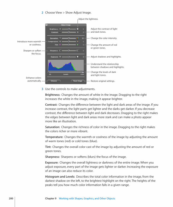
2 Choose View > Show Adjust Image.
Adjust the contrast of light and dark tones.
Change the color intensity.Introduce more warmth
or coolness. Change the amount of red or green tones.
Sharpen or soften the focus.
Adjust shadows and highlights.
Understand the relationship between shadows and highlights.
Change the levels of dark and light tones.
Restore original settings.
Adjust the lightness.
Enhance colors automatically.
3 Use the controls to make adjustments.
Brightness:� Changes the amount of white in the image. Dragging to the right increases the white in the image, making it appear brighter.
Contrast:� Changes the difference between the light and dark areas of the image. If you increase contrast, the light parts get lighter and the darks get darker. If you decrease contrast, the difference between light and dark decreases. Dragging to the right makes the edges between light and dark areas more stark and can make a photo appear more like an illustration.
Saturation:� Changes the richness of color in the image. Dragging to the right makes the colors richer or more vibrant.
Temperature:� Changes the warmth or coolness of the image by adjusting the amount of warm tones (red) or cold tones (blue).
Tint:� Changes the overall color cast of the image by adjusting the amount of red or green tones.
Sharpness:� Sharpens or softens (blurs) the focus of the image.
Exposure:� Changes the overall lightness or darkness of the entire image. When you adjust exposure, every part of the image gets lighter or darker. Increasing the exposure of an image can also reduce its color.
Histogram and Levels:� Describes the total color information in the image, from the darkest shadow on the left, to the brightest highlight on the right. The heights of the peaks tell you how much color information falls in a given range.
200 Chapter 9 Working with Shapes, Graphics, and Other Objects
Chapter 9 Working with Shapes, Graphics, and Other Objects 201
To set the dark level, drag the left slider toward the middle. Dragging the slider to Âthe right narrows the range of color and can bring more clarity to the shadows. The position of the slider determines how much information is in the darkest part of the image; any information to the left of the slider is omitted from the image. You may want to drag the slider just to the point that the histogram line shows a noticeable bump, signifying that detail is available.
To set the light level, drag the right slider toward the middle. Dragging the slider to Âthe left narrows the range of color and can bring more clarity to the highlights. The position of the slider determines how much information is in the lightest part of the image; any information to the right of the slider is omitted from the image. You may want to drag the slider just to the point that the histogram line shows a noticeable bump, signifying that detail is available.
Enhance:� Automatically adjusts the image by spreading the red, green, and blue tones evenly across the histogram.
4 To restore the original settings, click Reset Image.
To save any changes you made, save the document. The settings at the time you save the document are visible anytime you open the Adjust Image window.
Creating ShapesNumbers provides a variety of predrawn shapes you can add to spreadsheets, including circles, rectangles with square or rounded corners, stars, “speech bubbles,” arrows, and more. You can also create your own custom shapes or alter the lines and contours of a predrawn shape.
To learn how to Go to
Add a simple predefined shape “Adding a Predrawn Shape” on page 201
Draw your own shapes “Adding a Custom Shape” on page 202
Modify a shape’s contours “Editing Shapes” on page 203
Change a shape’s orientation, color, shadow, and more
“Manipulating, Arranging, and Changing the Look of Objects” on page 212
Adding a Predrawn ShapeYou can insert predrawn shapes, such as triangles, arrows, circles, and rectangles, to use as simple graphics.
Here are ways to add a predrawn shape:�Click Shapes in the toolbar, and then choose a shape from the pop-up menu. m
Choose Insert > Shape > m Shape.
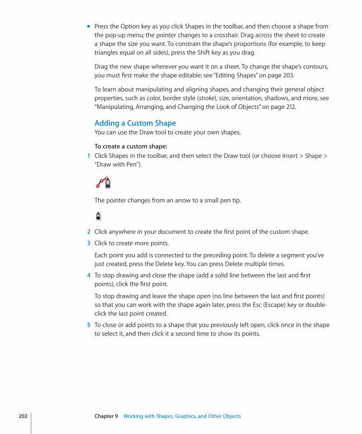
Press the Option key as you click Shapes in the toolbar, and then choose a shape from m
the pop-up menu; the pointer changes to a crosshair. Drag across the sheet to create a shape the size you want. To constrain the shape’s proportions (for example, to keep triangles equal on all sides), press the Shift key as you drag.
Drag the new shape wherever you want it on a sheet. To change the shape’s contours, you must first make the shape editable; see “Editing Shapes” on page 203.
To learn about manipulating and aligning shapes, and changing their general object properties, such as color, border style (stroke), size, orientation, shadows, and more, see “Manipulating, Arranging, and Changing the Look of Objects” on page 212.
Adding a Custom ShapeYou can use the Draw tool to create your own shapes.
To create a custom shape:� 1 Click Shapes in the toolbar, and then select the Draw tool (or choose Insert > Shape >
“Draw with Pen”).
The pointer changes from an arrow to a small pen tip.
2 Click anywhere in your document to create the first point of the custom shape.
3 Click to create more points.
Each point you add is connected to the preceding point. To delete a segment you’ve just created, press the Delete key. You can press Delete multiple times.
4 To stop drawing and close the shape (add a solid line between the last and first points), click the first point.
To stop drawing and leave the shape open (no line between the last and first points) so that you can work with the shape again later, press the Esc (Escape) key or double-click the last point created.
5 To close or add points to a shape that you previously left open, click once in the shape to select it, and then click it a second time to show its points.
202 Chapter 9 Working with Shapes, Graphics, and Other Objects
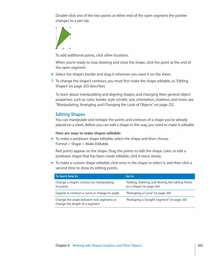
Chapter 9 Working with Shapes, Graphics, and Other Objects 203
Double-click one of the two points at either end of the open segment; the pointer changes to a pen tip.
To add additional points, click other locations.
When you’re ready to stop drawing and close the shape, click the point at the end of the open segment.
6 Select the shape’s border and drag it wherever you want it on the sheet.
7 To change the shape’s contours, you must first make the shape editable, as “Editing Shapes” on page 203 describes.
To learn about manipulating and aligning shapes, and changing their general object properties, such as color, border style (stroke), size, orientation, shadows, and more, see “Manipulating, Arranging, and Changing the Look of Objects” on page 212.
Editing ShapesYou can manipulate and reshape the points and contours of a shape you’ve already placed on a sheet. Before you can edit a shape in this way, you need to make it editable.
Here are ways to make shapes editable:�To make a predrawn shape editable, select the shape and then choose m
Format > Shape > Make Editable.
Red points appear on the shape. Drag the points to edit the shape. Later, to edit a predrawn shape that has been made editable, click it twice slowly.
To make a custom shape editable, click once in the shape to select it, and then click a m
second time to show its editing points.
To learn how to Go to
Change a shape’s contour by manipulating its points
“Adding, Deleting, and Moving the Editing Points on a Shape” on page 204
Expand or contract a curve or change its angle “Reshaping a Curve” on page 204
Change the angle between two segments or change the length of a segment
“Reshaping a Straight Segment” on page 205
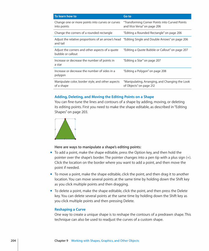
To learn how to Go to
Change one or more points into curves or curves into points
“Transforming Corner Points into Curved Points and Vice Versa” on page 206
Change the corners of a rounded rectangle “Editing a Rounded Rectangle” on page 206
Adjust the relative proportions of an arrow’s head and tail
“Editing Single and Double Arrows” on page 206
Adjust the corners and other aspects of a quote bubble or callout
“Editing a Quote Bubble or Callout” on page 207
Increase or decrease the number of points in a star
“Editing a Star” on page 207
Increase or decrease the number of sides in a polygon
“Editing a Polygon” on page 208
Manipulate color, border style, and other aspects of a shape
“Manipulating, Arranging, and Changing the Look of Objects” on page 212
Adding, Deleting, and Moving the Editing Points on a ShapeYou can fine-tune the lines and contours of a shape by adding, moving, or deleting its editing points. First you need to make the shape editable, as described in “Editing Shapes” on page 203.
Here are ways to manipulate a shape’s editing points:�To add a point, make the shape editable, press the Option key, and then hold the m
pointer over the shape’s border. The pointer changes into a pen tip with a plus sign (+). Click the location on the border where you want to add a point, and then move the point if needed.
To move a point, make the shape editable, click the point, and then drag it to another m
location. You can move several points at the same time by holding down the Shift key as you click multiple points and then dragging.
To delete a point, make the shape editable, click the point, and then press the Delete m
key. You can delete several points at the same time by holding down the Shift key as you click multiple points and then pressing Delete.
Reshaping a CurveOne way to create a unique shape is to reshape the contours of a predrawn shape. This technique can also be used to readjust the curves of a custom shape.
204 Chapter 9 Working with Shapes, Graphics, and Other Objects
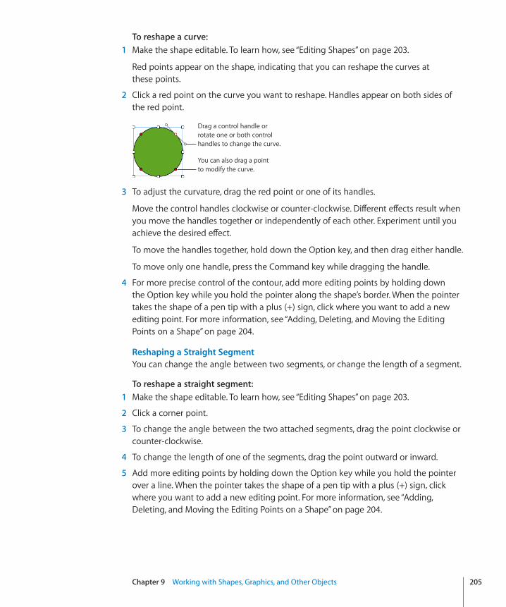
Chapter 9 Working with Shapes, Graphics, and Other Objects 205
To reshape a curve:� 1 Make the shape editable. To learn how, see “Editing Shapes” on page 203.
Red points appear on the shape, indicating that you can reshape the curves at these points.
2 Click a red point on the curve you want to reshape. Handles appear on both sides of the red point.
You can also drag a point to modify the curve.
Drag a control handle or rotate one or both control handles to change the curve.
3 To adjust the curvature, drag the red point or one of its handles.
Move the control handles clockwise or counter-clockwise. Different effects result when you move the handles together or independently of each other. Experiment until you achieve the desired effect.
To move the handles together, hold down the Option key, and then drag either handle.
To move only one handle, press the Command key while dragging the handle.
4 For more precise control of the contour, add more editing points by holding down the Option key while you hold the pointer along the shape’s border. When the pointer takes the shape of a pen tip with a plus (+) sign, click where you want to add a new editing point. For more information, see “Adding, Deleting, and Moving the Editing Points on a Shape” on page 204.
Reshaping a Straight SegmentYou can change the angle between two segments, or change the length of a segment.
To reshape a straight segment:� 1 Make the shape editable. To learn how, see “Editing Shapes” on page 203.
2 Click a corner point.
3 To change the angle between the two attached segments, drag the point clockwise or counter-clockwise.
4 To change the length of one of the segments, drag the point outward or inward.
5 Add more editing points by holding down the Option key while you hold the pointer over a line. When the pointer takes the shape of a pen tip with a plus (+) sign, click where you want to add a new editing point. For more information, see “Adding, Deleting, and Moving the Editing Points on a Shape” on page 204.
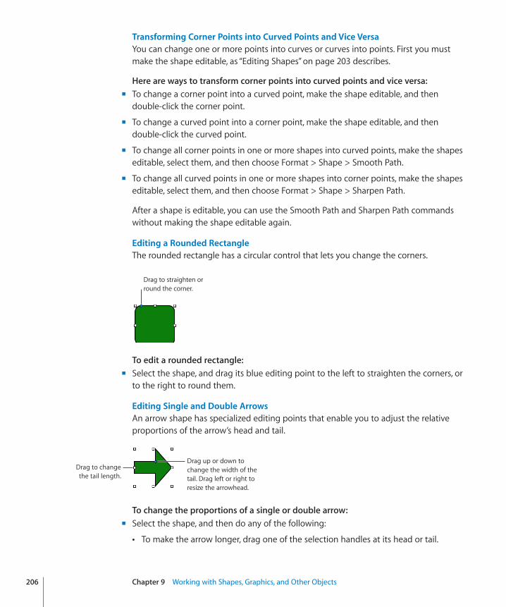
Transforming Corner Points into Curved Points and Vice VersaYou can change one or more points into curves or curves into points. First you must make the shape editable, as “Editing Shapes” on page 203 describes.
Here are ways to transform corner points into curved points and vice versa:�To change a corner point into a curved point, make the shape editable, and then m
double-click the corner point.
To change a curved point into a corner point, make the shape editable, and then m
double-click the curved point.
To change all corner points in one or more shapes into curved points, make the shapes m
editable, select them, and then choose Format > Shape > Smooth Path.
To change all curved points in one or more shapes into corner points, make the shapes m
editable, select them, and then choose Format > Shape > Sharpen Path.
After a shape is editable, you can use the Smooth Path and Sharpen Path commands without making the shape editable again.
Editing a Rounded RectangleThe rounded rectangle has a circular control that lets you change the corners.
Drag to straighten or round the corner.
To edit a rounded rectangle:�Select the shape, and drag its blue editing point to the left to straighten the corners, or m
to the right to round them.
Editing Single and Double ArrowsAn arrow shape has specialized editing points that enable you to adjust the relative proportions of the arrow’s head and tail.
Drag to change the tail length.
Drag up or down to change the width of the tail. Drag left or right to resize the arrowhead.
To change the proportions of a single or double arrow:�Select the shape, and then do any of the following: m
To make the arrow longer, drag one of the selection handles at its head or tail. Â
206 Chapter 9 Working with Shapes, Graphics, and Other Objects
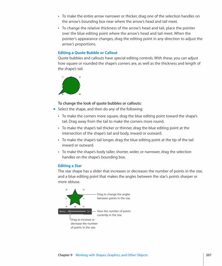
Chapter 9 Working with Shapes, Graphics, and Other Objects 207
To make the entire arrow narrower or thicker, drag one of the selection handles on Âthe arrow’s bounding box near where the arrow’s head and tail meet.
To change the relative thickness of the arrow’s head and tail, place the pointer Âover the blue editing point where the arrow’s head and tail meet. When the pointer’s appearance changes, drag the editing point in any direction to adjust the arrow’s proportions.
Editing a Quote Bubble or CalloutQuote bubbles and callouts have special editing controls. With these, you can adjust how square or rounded the shape’s corners are, as well as the thickness and length of the shape’s tail.
To change the look of quote bubbles or callouts:�Select the shape, and then do any of the following: m
To make the corners more square, drag the blue editing point toward the shape’s Âtail. Drag away from the tail to make the corners more round.
To make the shape’s tail thicker or thinner, drag the blue editing point at the Âintersection of the shape’s tail and body, inward or outward.
To make the shape’s tail longer, drag the blue editing point at the tip of the tail Âinward or outward.
To make the shape’s body taller, shorter, wider, or narrower, drag the selection Âhandles on the shape’s bounding box.
Editing a StarThe star shape has a slider that increases or decreases the number of points in the star, and a blue editing point that makes the angles between the star’s points sharper or more obtuse.
View the number of points currently in the star.
Drag to increase or decrease the number of points in the star.
Drag to change the angles between points in the star.
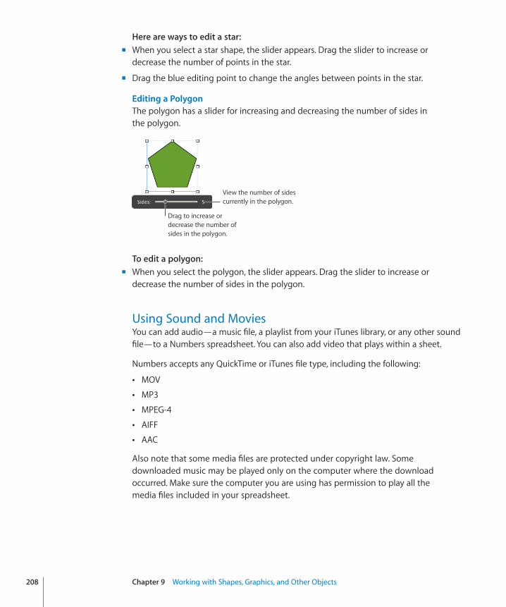
Here are ways to edit a star:�When you select a star shape, the slider appears. Drag the slider to increase or m
decrease the number of points in the star.
Drag the blue editing point to change the angles between points in the star. m
Editing a PolygonThe polygon has a slider for increasing and decreasing the number of sides in the polygon.
Drag to increase or decrease the number of sides in the polygon.
View the number of sides currently in the polygon.
To edit a polygon:�When you select the polygon, the slider appears. Drag the slider to increase or m
decrease the number of sides in the polygon.
Using Sound and MoviesYou can add audio—a music file, a playlist from your iTunes library, or any other sound file—to a Numbers spreadsheet. You can also add video that plays within a sheet.
Numbers accepts any QuickTime or iTunes file type, including the following:
MOV Â
MP3 Â
MPEG-4 Â
AIFF Â
AAC Â
Also note that some media files are protected under copyright law. Some downloaded music may be played only on the computer where the download occurred. Make sure the computer you are using has permission to play all the media files included in your spreadsheet.
208 Chapter 9 Working with Shapes, Graphics, and Other Objects
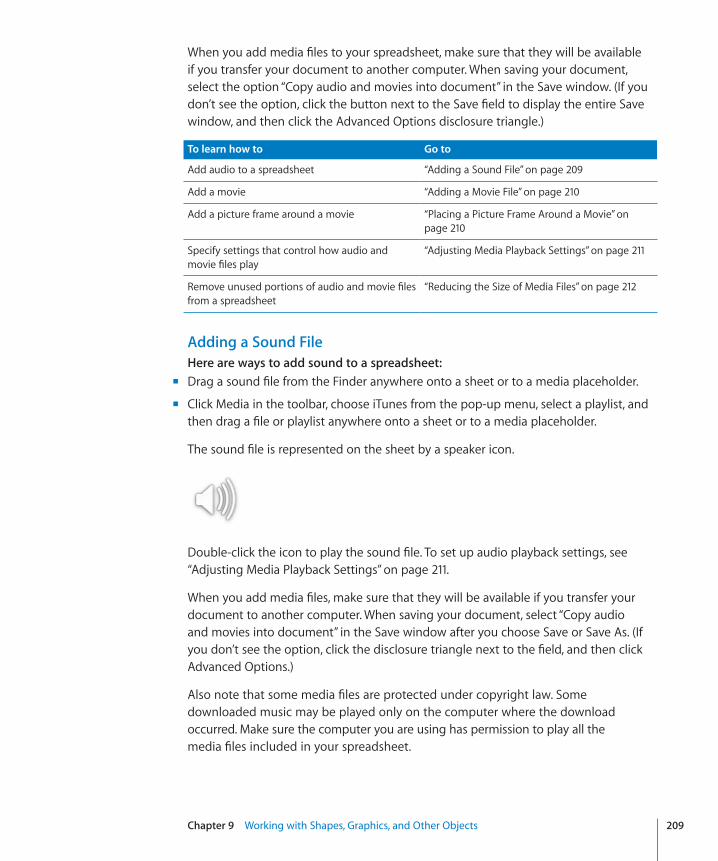
Chapter 9 Working with Shapes, Graphics, and Other Objects 209
When you add media files to your spreadsheet, make sure that they will be available if you transfer your document to another computer. When saving your document, select the option “Copy audio and movies into document” in the Save window. (If you don’t see the option, click the button next to the Save field to display the entire Save window, and then click the Advanced Options disclosure triangle.)
To learn how to Go to
Add audio to a spreadsheet “Adding a Sound File” on page 209
Add a movie “Adding a Movie File” on page 210
Add a picture frame around a movie “Placing a Picture Frame Around a Movie” on page 210
Specify settings that control how audio and movie files play
“Adjusting Media Playback Settings” on page 211
Remove unused portions of audio and movie files from a spreadsheet
“Reducing the Size of Media Files” on page 212
Adding a Sound FileHere are ways to add sound to a spreadsheet:�Drag a sound file from the Finder anywhere onto a sheet or to a media placeholder. m
Click Media in the toolbar, choose iTunes from the pop-up menu, select a playlist, and m
then drag a file or playlist anywhere onto a sheet or to a media placeholder.
The sound file is represented on the sheet by a speaker icon.
Double-click the icon to play the sound file. To set up audio playback settings, see “Adjusting Media Playback Settings” on page 211.
When you add media files, make sure that they will be available if you transfer your document to another computer. When saving your document, select “Copy audio and movies into document” in the Save window after you choose Save or Save As. (If you don’t see the option, click the disclosure triangle next to the field, and then click Advanced Options.)
Also note that some media files are protected under copyright law. Some downloaded music may be played only on the computer where the download occurred. Make sure the computer you are using has permission to play all the media files included in your spreadsheet.
Adding a Movie FileHere are ways to add a movie to a spreadsheet:�Drag a movie file from the Finder to a sheet or to a media placeholder. m
Click Media in the toolbar, and then click Movies in the Media Browser. Select a file, and m
then drag it to a sheet or to a media placeholder.
Choose Insert > Choose, and then navigate to the movie file you want. Select it, and m
then click Insert. Drag the movie where you want it on a sheet.
To learn about further adjustments you can make to control movie playback, see “Adjusting Media Playback Settings” on page 211.
Also note that some media files are protected under copyright law. Some downloaded music may be played only on the computer where the download occurred. Make sure the computer you are using has permission to play all the media files included in your spreadsheet.
When you add media files to your spreadsheet, make sure that they will be available if you transfer your document to another computer. When saving your document, select “Copy audio and movies into document” in the Save window after you choose Save or Save As. (If you don’t see the option, click the disclosure triangle next to the field, and then click Advanced Options.)
Placing a Picture Frame Around a MoviePlacing a picture frame around a movie is an attractive way to display it in a spreadsheet. To add a picture frame, you use the Stroke settings in the Graphic inspector.
To frame a movie:� 1 Select it, and then click the Inspector button in the toolbar to open the Inspector
window. Click the Graphic inspector button in the Inspector window.
2 Choose Picture Frame from the Stroke pop-up menu.
3 Click the picture frame that appears below the Stroke pop-up menu, and choose a frame style.
4 Drag the Scale slider or specify a percentage to set the thickness of the picture frame.
See “Framing Objects” on page 222 for more information about picture frames.
210 Chapter 9 Working with Shapes, Graphics, and Other Objects
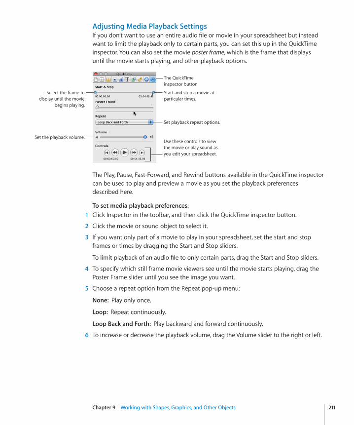
Chapter 9 Working with Shapes, Graphics, and Other Objects 211
Adjusting Media Playback SettingsIf you don’t want to use an entire audio file or movie in your spreadsheet but instead want to limit the playback only to certain parts, you can set this up in the QuickTime inspector. You can also set the movie poster frame, which is the frame that displays until the movie starts playing, and other playback options.
Use these controls to view the movie or play sound as you edit your spreadsheet.
Start and stop a movie at particular times.
Set playback repeat options.
Set the playback volume.
Select the frame to display until the movie
begins playing.
The QuickTime inspector button
The Play, Pause, Fast-Forward, and Rewind buttons available in the QuickTime inspector can be used to play and preview a movie as you set the playback preferences described here.
To set media playback preferences:� 1 Click Inspector in the toolbar, and then click the QuickTime inspector button.
2 Click the movie or sound object to select it.
3 If you want only part of a movie to play in your spreadsheet, set the start and stop frames or times by dragging the Start and Stop sliders.
To limit playback of an audio file to only certain parts, drag the Start and Stop sliders.
4 To specify which still frame movie viewers see until the movie starts playing, drag the Poster Frame slider until you see the image you want.
5 Choose a repeat option from the Repeat pop-up menu:
None:� Play only once.
Loop:� Repeat continuously.
Loop Back and Forth:� Play backward and forward continuously.
6 To increase or decrease the playback volume, drag the Volume slider to the right or left.
Reducing the Size of Media FilesIncluding large sound and movie files in a Numbers spreadsheet can make the entire document file size very large. If you’re using only a portion of the sound or movie file in your spreadsheet, you can remove the unused portions of the audio or video file to make the Numbers file smaller. You can choose either to reduce the size of individual media files or to reduce the size of all the media files in the document that are not being used in full.
Before you reduce the movie or audio files, you must save them as part of your document. Choose File > Save, click Advanced Options, make sure that “Copy audio and movies into document” is selected, and then click Save. For more details about saving spreadsheets, see “Saving a Spreadsheet” on page 32.
Here are ways to reduce the file size of your spreadsheet:To reduce the size of an individual media file in your document, select a sound or m
movie file for which you have set the Start and Stop sliders to exclude some part of the file, and then choose Format > Image > Reduce Media File Size.
To reduce the size of all the media files in your document, make sure no sound, movie, m
or image file is selected, and then choose File > Reduce File Size.
After reducing the size of your sound or video file, you won’t be able to restore the file to its original length or listen to or view the parts that you have excluded. To restore the entire file, you must add the file again.
Some types of movie files may not be reducible in this way.
To learn about reducing the size of image files, see “Reducing Image File Sizes” on page 198.
Manipulating, Arranging, and Changing the Look of ObjectsIn general, the way you select, arrange, and manipulate objects in Numbers works the same, whether you’re working with images, shapes, movies, tables, chart elements, or text boxes. For most objects, you use the same controls to resize and reorient them, as well as to add shadows, reflections, border styles (stroke), fill color or image, and more.
To learn how to Go to
Select one or more objects so you can edit them “Selecting Objects” on page 213
Copy or duplicate an object “Copying or Duplicating Objects” on page 213
Remove an object “Deleting Objects” on page 214
212 Chapter 9 Working with Shapes, Graphics, and Other Objects
Chapter 9 Working with Shapes, Graphics, and Other Objects 213
To learn how to Go to
Arrange objects on a sheet, group them, and lock them
“Moving and Positioning Objects” on page 214
Resize objects, change their orientation, modify their borders, and perform other editing operations
“Modifying Objects” on page 219
Fill objects with a solid color, color gradients, or images
“Filling Objects with Colors or Images” on page 225
Selecting ObjectsBefore you can move, modify, or perform other operations on objects, you must select them. A selected object has handles that let you move or manipulate the object.
Here are ways to select and deselect objects:�To select a table, click its name in the Sheets pane. For other table selection m
techniques, see “Selecting Tables and Their Components” on page 55.
To select other single objects, click anywhere in the object (to select an object that has no fill, click the edge).
To select several objects on a sheet, hold down the Shift key as you click objects. m
To select all the objects on a sheet, click the sheet and press Command-A. m
To select an object that’s part of a group, you must first ungroup the objects. Select m
the group, and then choose Arrange > Ungroup.
To deselect objects in a group of selected objects, hold down the Command key and m
then click objects you want to deselect.
Copying or Duplicating ObjectsThe technique you use to copy an object depends on where you want to place the copy. When the copy will be placed far from the original or in another document, copying and pasting is generally easier. When you’re working with an object that will be placed near the original, duplicating is generally easier.
Here are ways to copy objects:�To copy and paste an object, select it, and then choose Edit > Copy. Click where you m
want the copy to appear. Choose Edit > Paste.
To duplicate an object on a sheet, hold down the Option key while you drag the object. m
You can also select the object and choose Edit > Duplicate. The copy appears on top of the original, slightly offset. Drag the copy to the desired location.
To copy an image between Numbers documents, select the image and drag its icon m
from the File Info field in the Metrics Inspector to a sheet in the other Numbers file.
Deleting ObjectsTo delete objects:�Select the object(s) and press the Delete key. m
If you accidentally delete an object, choose Edit > Undo Delete.
Moving and Positioning ObjectsNumbers provides several tools to help you arrange items on a sheet with great precision, including customizable alignment guides. Objects can be grouped together, making it easier to manipulate sets of objects, and locked into position to prevent them from being moved while you work. In addition, objects can be layered (overlapped) to create the effect of depth.
Here are ways to manipulate objects directly:�To move a table to a new location on a sheet, use the techniques described in “ m Moving Tables” on page 52.
To move other objects, drag them. Avoid dragging objects by their selection handles because you may inadvertently resize them.
To precisely align objects as you drag them around, you can use alignment guides. See m
“Using Alignment Guides” on page 216 for details.
To constrain the object’s motion to horizontal, vertical, or a 45-degree angle, start m
dragging the object while holding down the Shift key.
To move a selected object in small increments, press one of the arrow keys, causing m
the object to move a point at a time. To move the object ten points at a time, hold down the Shift key while pressing an arrow key.
To show the position of the object when you move it, choose Numbers > Preferences, m
and then select “Show size and position when moving objects” in the General pane.
To move text or an object inside another object, select the object and choose Edit > m
Cut. Place the insertion point where you want the object to appear, and then choose Edit > Paste.
To learn how to Go to
Change the order of overlapping objects “Moving an Object Forward or Backward (Layering Objects)” on page 215
Align objects “Quickly Aligning Objects Relative to One Another” on page 215
Use alignment guides to align objects “Using Alignment Guides” on page 216
214 Chapter 9 Working with Shapes, Graphics, and Other Objects
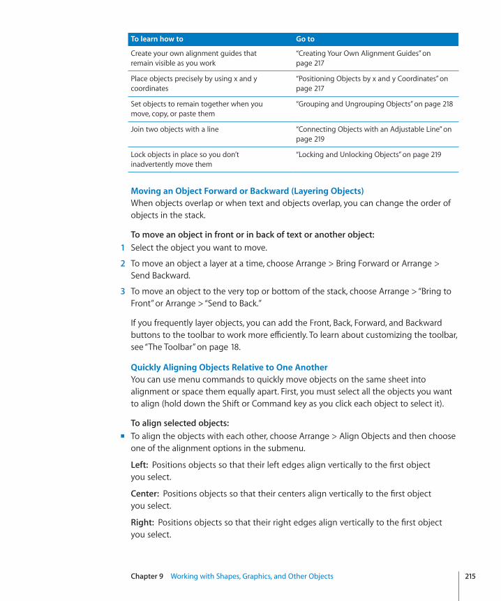
Chapter 9 Working with Shapes, Graphics, and Other Objects 215
To learn how to Go to
Create your own alignment guides that remain visible as you work
“Creating Your Own Alignment Guides” on page 217
Place objects precisely by using x and y coordinates
“Positioning Objects by x and y Coordinates” on page 217
Set objects to remain together when you move, copy, or paste them
“Grouping and Ungrouping Objects” on page 218
Join two objects with a line “Connecting Objects with an Adjustable Line” on page 219
Lock objects in place so you don’t inadvertently move them
“Locking and Unlocking Objects” on page 219
Moving an Object Forward or Backward (Layering Objects)When objects overlap or when text and objects overlap, you can change the order of objects in the stack.
To move an object in front or in back of text or another object:� 1 Select the object you want to move.
2 To move an object a layer at a time, choose Arrange > Bring Forward or Arrange > Send Backward.
3 To move an object to the very top or bottom of the stack, choose Arrange > “Bring to Front” or Arrange > “Send to Back.”
If you frequently layer objects, you can add the Front, Back, Forward, and Backward buttons to the toolbar to work more efficiently. To learn about customizing the toolbar, see “The Toolbar” on page 18.
Quickly Aligning Objects Relative to One AnotherYou can use menu commands to quickly move objects on the same sheet into alignment or space them equally apart. First, you must select all the objects you want to align (hold down the Shift or Command key as you click each object to select it).
To align selected objects:�To align the objects with each other, choose Arrange > Align Objects and then choose m
one of the alignment options in the submenu.
Left:� Positions objects so that their left edges align vertically to the first object you select.
Center:� Positions objects so that their centers align vertically to the first object you select.
Right:� Positions objects so that their right edges align vertically to the first object you select.
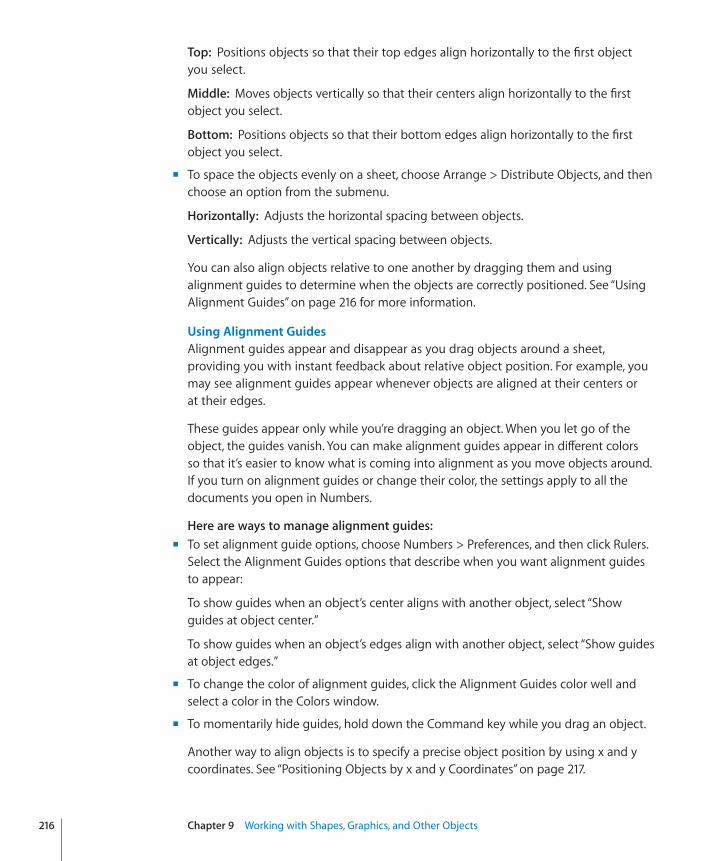
Top:� Positions objects so that their top edges align horizontally to the first object you select.
Middle:� Moves objects vertically so that their centers align horizontally to the first object you select.
Bottom:� Positions objects so that their bottom edges align horizontally to the first object you select.
To space the objects evenly on a sheet, choose Arrange > Distribute Objects, and then m
choose an option from the submenu.
Horizontally:� Adjusts the horizontal spacing between objects.
Vertically:� Adjusts the vertical spacing between objects.
You can also align objects relative to one another by dragging them and using alignment guides to determine when the objects are correctly positioned. See “Using Alignment Guides” on page 216 for more information.
Using Alignment GuidesAlignment guides appear and disappear as you drag objects around a sheet, providing you with instant feedback about relative object position. For example, you may see alignment guides appear whenever objects are aligned at their centers or at their edges.
These guides appear only while you’re dragging an object. When you let go of the object, the guides vanish. You can make alignment guides appear in different colors so that it’s easier to know what is coming into alignment as you move objects around. If you turn on alignment guides or change their color, the settings apply to all the documents you open in Numbers.
Here are ways to manage alignment guides:�To set alignment guide options, choose Numbers > Preferences, and then click Rulers. m
Select the Alignment Guides options that describe when you want alignment guides to appear:
To show guides when an object’s center aligns with another object, select “Show guides at object center.”
To show guides when an object’s edges align with another object, select “Show guides at object edges.”
To change the color of alignment guides, click the Alignment Guides color well and m
select a color in the Colors window.
To momentarily hide guides, hold down the Command key while you drag an object. m
Another way to align objects is to specify a precise object position by using x and y coordinates. See “Positioning Objects by x and y Coordinates” on page 217.
216 Chapter 9 Working with Shapes, Graphics, and Other Objects
Chapter 9 Working with Shapes, Graphics, and Other Objects 217
Creating your own alignment guides wherever you need them can also help you place objects. See “Creating Your Own Alignment Guides” on page 217.
Creating Your Own Alignment GuidesYou can create static alignment guides to help you align objects on a sheet. These alignment guides don’t appear and disappear as you drag objects but remain visible while you’re working, even if you leave the sheet and then return to it later.
To create an alignment guide:� 1 Click View in the toolbar, and then choose Show Rulers.
Note: Alignment guides can’t be created if you are editing text. Stop editing text by selecting an object or clicking the sheet.
2 Place the pointer over a ruler and drag onto a sheet. An alignment guide appears.
3 Drag the guide where you want it on the sheet.
4 To remove an alignment guide that you’ve created, drag it off the edge of the sheet.
You can also specify x and y coordinates to place objects precisely. See “Positioning Objects by x and y Coordinates” on page 217.
Positioning Objects by x and y CoordinatesYou can place objects precisely where you want them on a sheet by specifying spatial coordinates using the ruler measurements.
To specify an object’s position by its x and y coordinates:� 1 Select the object you want to position.
2 Click Inspector in the toolbar, and then click the Metrics inspector button.
3 Enter x and y values (in ruler measurements) in the Position fields.
The specified coordinates determine the position of the upper-left corner of the object’s container box. If an object is rotated, the x and y coordinates specify the upper-left corner of the container box of the rotated object, which may be a different size from the original.
The x value is measured from the left edge of the sheet. Â
The y value is measured from the top edge of the sheet. Â
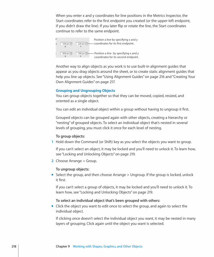
When you enter x and y coordinates for line positions in the Metrics Inspector, the Start coordinates refer to the first endpoint you created (or the upper-left endpoint, if you didn’t draw the line). If you later flip or rotate the line, the Start coordinates continue to refer to the same endpoint.
Position a line by specifying x and y coordinates for its first endpoint.
Position a line by specifying x and y coordinates for its second endpoint.
Another way to align objects as you work is to use built-in alignment guides that appear as you drag objects around the sheet, or to create static alignment guides that help you line up objects. See “Using Alignment Guides” on page 216 and “Creating Your Own Alignment Guides” on page 217.
Grouping and Ungrouping ObjectsYou can group objects together so that they can be moved, copied, resized, and oriented as a single object.
You can edit an individual object within a group without having to ungroup it first.
Grouped objects can be grouped again with other objects, creating a hierarchy or “nesting” of grouped objects. To select an individual object that’s nested in several levels of grouping, you must click it once for each level of nesting.
To group objects:� 1 Hold down the Command (or Shift) key as you select the objects you want to group.
If you can’t select an object, it may be locked and you’ll need to unlock it. To learn how, see “Locking and Unlocking Objects” on page 219.
2 Choose Arrange > Group.
To ungroup objects:�Select the group, and then choose Arrange > Ungroup. If the group is locked, unlock m
it first.
If you can’t select a group of objects, it may be locked and you’ll need to unlock it. To learn how, see “Locking and Unlocking Objects” on page 219.
To select an individual object that’s been grouped with others:�Click the object you want to edit once to select the group, and again to select the m
individual object.
If clicking once doesn’t select the individual object you want, it may be nested in many layers of grouping. Click again until the object you want is selected.
218 Chapter 9 Working with Shapes, Graphics, and Other Objects
Chapter 9 Working with Shapes, Graphics, and Other Objects 219
Connecting Objects with an Adjustable LineWhen you want to join two objects with a line, the easiest way is to use a connection line (rather than creating a separate line as a shape). Two objects joined by a connection line remain joined even if you reposition the objects.
To join two objects with a connection line:� 1 Hold down the Command key while you select the two objects you want to join, and
then choose Insert > Connection Line.
A straight line appears, connecting the selected objects. You can move the object separately, and the connection line shrinks, stretches, and changes its position to keep the objects connected.
2 To make the line curved, drag the white editing point near the center of the line.
If you drag the objects into different positions on a sheet, the curvature of the line adjusts to keep the objects connected.
3 To create a gap between the end of the line and one of the connected objects, so that they aren’t actually touching, drag the blue editing point at the end of the line away from the object it’s touching.
The line maintains the gap between itself and the connected object as you move the objects around.
4 To change the line color, style, thickness, or endpoints, format it using the controls in the format bar or Graphic inspector, as you would for any other line. For more detailed information about changing these attributes, see “Modifying Objects” on page 219.
Locking and Unlocking ObjectsYou can lock objects to avoid inadvertently moving them as you work.
After you lock individual or grouped objects, you can’t move, delete, or modify them in any way until you unlock them. However, a locked object can be selected, copied, or duplicated; when you copy or duplicate a locked object, the new object is also locked.
To lock an object:�Select the objects you want to lock, and then choose Arrange > Lock. m
To unlock an object:�Select the objects you want to unlock, and then choose Arrange > Unlock. m
Modifying ObjectsYou can resize objects, change their orientation, modify their border styles, add shadows and reflections to them, and adjust their opacity.
To learn how to Go to
Change an object’s size “Resizing Objects” on page 220
Flip or rotate an object “Flipping and Rotating Objects” on page 220
Format a border around objects “Changing the Style of Borders” on page 221
Place a picture frame around an object “Framing Objects” on page 222
Add shadows to create an appearance of depth “Adding Shadows” on page 223
Add a reflection that reflects vertically downward “Adding a Reflection” on page 224
Make objects more or less opaque “Adjusting Opacity” on page 224
Resizing ObjectsYou can resize an object by dragging its handles or typing exact dimensions.
Here are ways to resize objects:�To resize an object by dragging, select the object and then drag one of its m
selection handles. To resize an object in one direction, drag a side handle instead of a corner handle.
To resize the object from its center, press the Option key as you drag.
To maintain an object’s proportions, hold down the Shift key as you drag. You can also click Inspector in the toolbar, click the Metrics inspector button, and then select “Constrain proportions” before dragging.
To show the size of an object when you drag a selection handle, choose Numbers > Preferences, and then select “Show size and position when moving objects” in the General pane.
To resize an object using exact proportions, select the object, click Inspector in the m
toolbar, click the Metrics inspector button, and then use the Width and Height controls.
To resize several objects at once, select the objects, click Inspector in the toolbar, click m
the Metrics inspector button, and then type new values in the Width and Height fields.
Select the object, and then click Original Size in the Metrics inspector. m
If you resized a very large image file but need to use only the smaller version in your spreadsheet, you can have Numbers keep only a smaller copy of the image, thus reducing the overall size of your document. See “Reducing Image File Sizes” on page 198.
Flipping and Rotating ObjectsYou can flip or rotate any object. For example, if you have an image of an arrow that you want to use in your document, but you need it to point in a different direction, you can reverse its direction vertically or horizontally, or point it at any angle.
220 Chapter 9 Working with Shapes, Graphics, and Other Objects
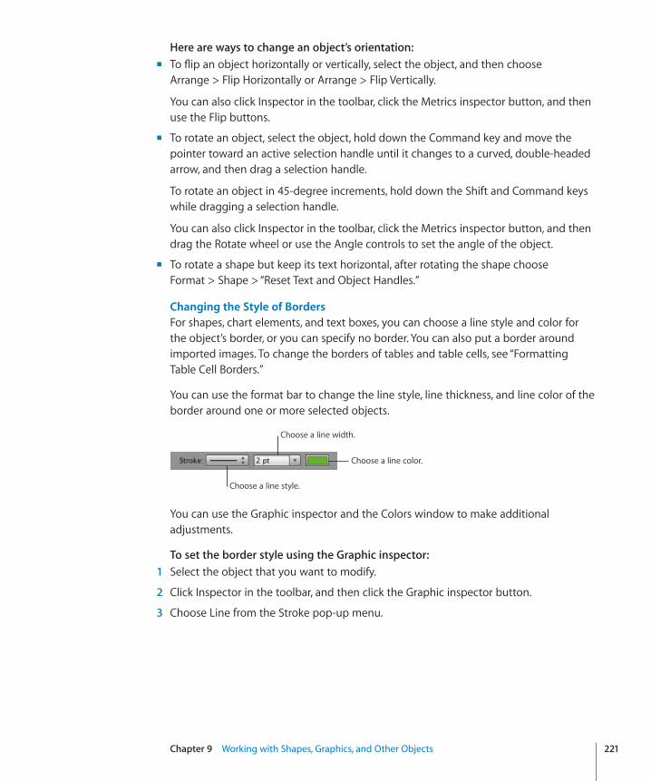
Chapter 9 Working with Shapes, Graphics, and Other Objects 221
Here are ways to change an object’s orientation:�To flip an object horizontally or vertically, select the object, and then choose m
Arrange > Flip Horizontally or Arrange > Flip Vertically.
You can also click Inspector in the toolbar, click the Metrics inspector button, and then use the Flip buttons.
To rotate an object, select the object, hold down the Command key and move the m
pointer toward an active selection handle until it changes to a curved, double-headed arrow, and then drag a selection handle.
To rotate an object in 45-degree increments, hold down the Shift and Command keys while dragging a selection handle.
You can also click Inspector in the toolbar, click the Metrics inspector button, and then drag the Rotate wheel or use the Angle controls to set the angle of the object.
To rotate a shape but keep its text horizontal, after rotating the shape choose m
Format > Shape > “Reset Text and Object Handles.”
Changing the Style of BordersFor shapes, chart elements, and text boxes, you can choose a line style and color for the object’s border, or you can specify no border. You can also put a border around imported images. To change the borders of tables and table cells, see “Formatting Table Cell Borders.”
You can use the format bar to change the line style, line thickness, and line color of the border around one or more selected objects.
Choose a line color.
Choose a line style.
Choose a line width.
You can use the Graphic inspector and the Colors window to make additional adjustments.
To set the border style using the Graphic inspector:� 1 Select the object that you want to modify.
2 Click Inspector in the toolbar, and then click the Graphic inspector button.
3 Choose Line from the Stroke pop-up menu.
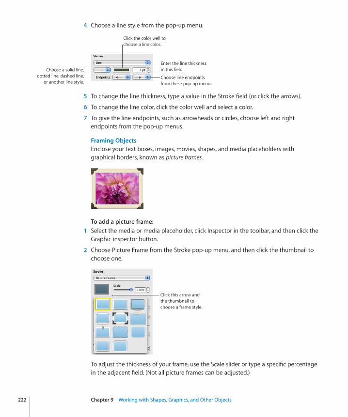
4 Choose a line style from the pop-up menu.
Enter the line thickness in this field.
Choose line endpoints from these pop-up menus.
Choose a solid line, dotted line, dashed line,
or another line style.
Click the color well to choose a line color.
5 To change the line thickness, type a value in the Stroke field (or click the arrows).
6 To change the line color, click the color well and select a color.
7 To give the line endpoints, such as arrowheads or circles, choose left and right endpoints from the pop-up menus.
Framing ObjectsEnclose your text boxes, images, movies, shapes, and media placeholders with graphical borders, known as picture frames.
To add a picture frame:� 1 Select the media or media placeholder, click Inspector in the toolbar, and then click the
Graphic inspector button.
2 Choose Picture Frame from the Stroke pop-up menu, and then click the thumbnail to choose one.
Click this arrow and the thumbnail to choose a frame style.
To adjust the thickness of your frame, use the Scale slider or type a specific percentage in the adjacent field. (Not all picture frames can be adjusted.)
222 Chapter 9 Working with Shapes, Graphics, and Other Objects
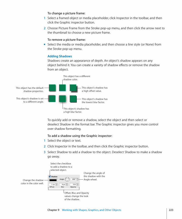
Chapter 9 Working with Shapes, Graphics, and Other Objects 223
To change a picture frame:� 1 Select a framed object or media placeholder, click Inspector in the toolbar, and then
click the Graphic inspector button.
2 Choose Picture Frame from the Stroke pop-up menu, and then click the arrow next to the thumbnail to choose a new picture frame.
To remove a picture frame:�Select the media or media placeholder, and then choose a line style (or None) from m
the Stroke pop-up menu.
Adding ShadowsShadows create an appearance of depth. An object’s shadow appears on any object behind it. You can create a variety of shadow effects or remove the shadow from an object.
This object has the default shadow properties.
This object’s shadow is set to a different angle.
This object’s shadow has a high offset value.
This object’s shadow has the lowest blur factor.
This object has a different shadow color.
This object’s shadow has a high blur factor.
To quickly add or remove a shadow, select the object and then select or deselect Shadow in the format bar. The Graphic inspector gives you more control over shadow formatting.
To add a shadow using the Graphic inspector:� 1 Select the object or text.
2 Click Inspector in the toolbar, and then click the Graphic inspector button.
3 Select Shadow to add a shadow to the object. Deselect Shadow to make a shadow go away.
Change the shadow color in the color well.
Change the angle of the shadow with the Angle wheel.
Offset, Blur, and Opacity values change the look of the shadow.
Select the checkbox to add a shadow to a selected object.
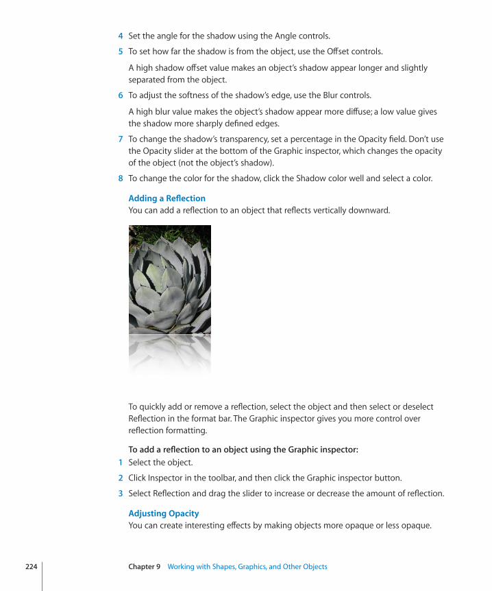
4 Set the angle for the shadow using the Angle controls.
5 To set how far the shadow is from the object, use the Offset controls.
A high shadow offset value makes an object’s shadow appear longer and slightly separated from the object.
6 To adjust the softness of the shadow’s edge, use the Blur controls.
A high blur value makes the object’s shadow appear more diffuse; a low value gives the shadow more sharply defined edges.
7 To change the shadow’s transparency, set a percentage in the Opacity field. Don’t use the Opacity slider at the bottom of the Graphic inspector, which changes the opacity of the object (not the object’s shadow).
8 To change the color for the shadow, click the Shadow color well and select a color.
Adding a ReflectionYou can add a reflection to an object that reflects vertically downward.
To quickly add or remove a reflection, select the object and then select or deselect Reflection in the format bar. The Graphic inspector gives you more control over reflection formatting.
To add a reflection to an object using the Graphic inspector: 1 Select the object.
2 Click Inspector in the toolbar, and then click the Graphic inspector button.
3 Select Reflection and drag the slider to increase or decrease the amount of reflection.
Adjusting OpacityYou can create interesting effects by making objects more opaque or less opaque.
224 Chapter 9 Working with Shapes, Graphics, and Other Objects
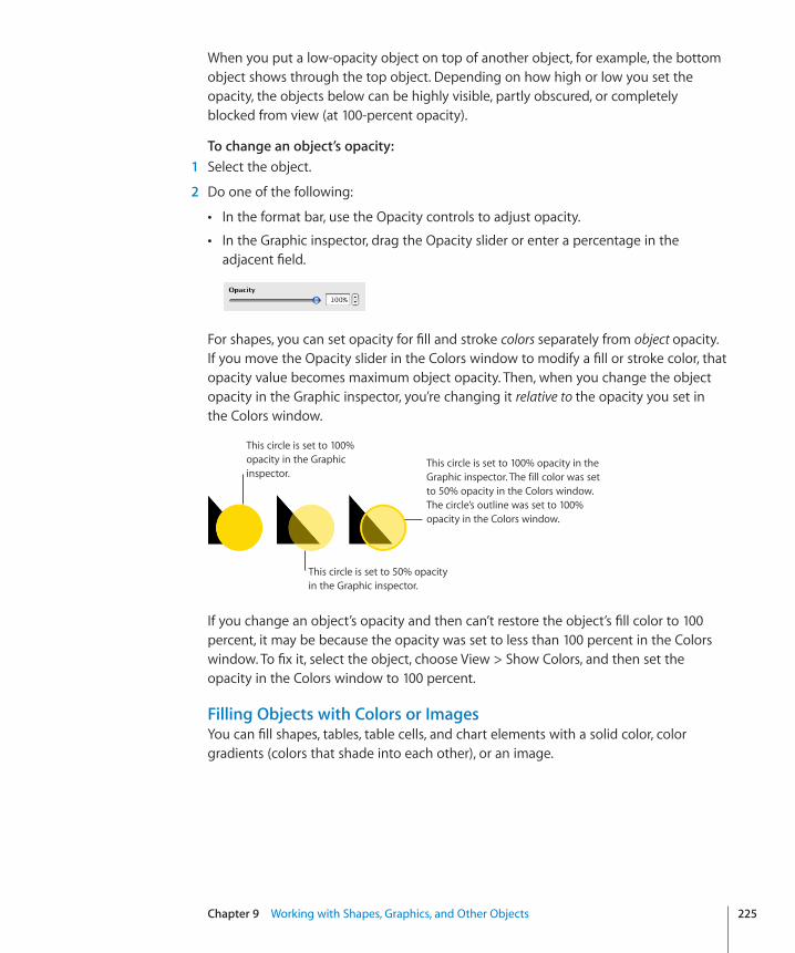
Chapter 9 Working with Shapes, Graphics, and Other Objects 225
When you put a low-opacity object on top of another object, for example, the bottom object shows through the top object. Depending on how high or low you set the opacity, the objects below can be highly visible, partly obscured, or completely blocked from view (at 100-percent opacity).
To change an object’s opacity:� 1 Select the object.
2 Do one of the following:
In the format bar, use the Opacity controls to adjust opacity. Â
In the Graphic inspector, drag the Opacity slider or enter a percentage in the Âadjacent field.
For shapes, you can set opacity for fill and stroke colors separately from object opacity. If you move the Opacity slider in the Colors window to modify a fill or stroke color, that opacity value becomes maximum object opacity. Then, when you change the object opacity in the Graphic inspector, you’re changing it relative to the opacity you set in the Colors window.
This circle is set to 100% opacity in the Graphic inspector. The fill color was set to 50% opacity in the Colors window. The circle’s outline was set to 100% opacity in the Colors window.
This circle is set to 100% opacity in the Graphic inspector.
This circle is set to 50% opacity in the Graphic inspector.
If you change an object’s opacity and then can’t restore the object’s fill color to 100 percent, it may be because the opacity was set to less than 100 percent in the Colors window. To fix it, select the object, choose View > Show Colors, and then set the opacity in the Colors window to 100 percent.
Filling Objects with Colors or ImagesYou can fill shapes, tables, table cells, and chart elements with a solid color, color gradients (colors that shade into each other), or an image.
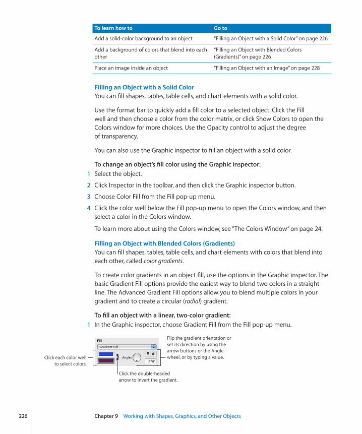
To learn how to Go to
Add a solid-color background to an object “Filling an Object with a Solid Color” on page 226
Add a background of colors that blend into each other
“Filling an Object with Blended Colors (Gradients)” on page 226
Place an image inside an object “Filling an Object with an Image” on page 228
Filling an Object with a Solid ColorYou can fill shapes, tables, table cells, and chart elements with a solid color.
Use the format bar to quickly add a fill color to a selected object. Click the Fill well and then choose a color from the color matrix, or click Show Colors to open the Colors window for more choices. Use the Opacity control to adjust the degree of transparency.
You can also use the Graphic inspector to fill an object with a solid color.
To change an object’s fill color using the Graphic inspector: 1 Select the object.
2 Click Inspector in the toolbar, and then click the Graphic inspector button.
3 Choose Color Fill from the Fill pop-up menu.
4 Click the color well below the Fill pop-up menu to open the Colors window, and then select a color in the Colors window.
To learn more about using the Colors window, see “The Colors Window” on page 24.
Filling an Object with Blended Colors (Gradients)You can fill shapes, tables, table cells, and chart elements with colors that blend into each other, called color gradients.
To create color gradients in an object fill, use the options in the Graphic inspector. The basic Gradient Fill options provide the easiest way to blend two colors in a straight line. The Advanced Gradient Fill options allow you to blend multiple colors in your gradient and to create a circular (radial) gradient.
To fill an object with a linear, two-color gradient: 1 In the Graphic inspector, choose Gradient Fill from the Fill pop-up menu.
Click the double-headed arrow to invert the gradient.
Flip the gradient orientation or set its direction by using the arrow buttons or the Angle wheel, or by typing a value.Click each color well
to select colors.
226 Chapter 9 Working with Shapes, Graphics, and Other Objects
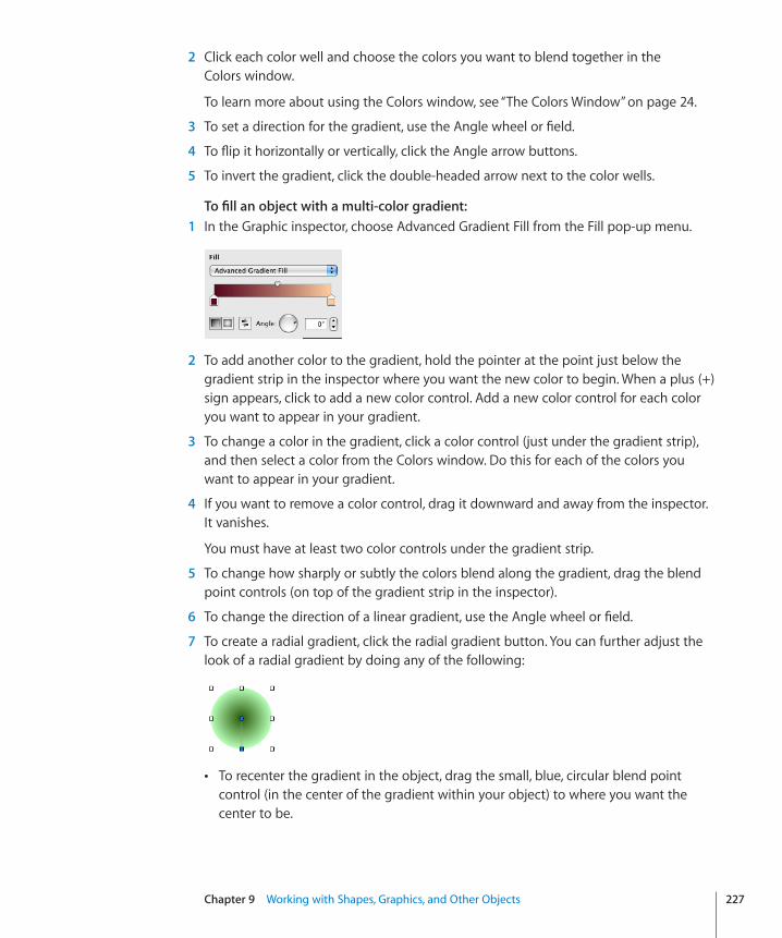
Chapter 9 Working with Shapes, Graphics, and Other Objects 227
2 Click each color well and choose the colors you want to blend together in the Colors window.
To learn more about using the Colors window, see “The Colors Window” on page 24.
3 To set a direction for the gradient, use the Angle wheel or field.
4 To flip it horizontally or vertically, click the Angle arrow buttons.
5 To invert the gradient, click the double-headed arrow next to the color wells.
To fill an object with a multi-color gradient: 1 In the Graphic inspector, choose Advanced Gradient Fill from the Fill pop-up menu.
2 To add another color to the gradient, hold the pointer at the point just below the gradient strip in the inspector where you want the new color to begin. When a plus (+) sign appears, click to add a new color control. Add a new color control for each color you want to appear in your gradient.
3 To change a color in the gradient, click a color control (just under the gradient strip), and then select a color from the Colors window. Do this for each of the colors you want to appear in your gradient.
4 If you want to remove a color control, drag it downward and away from the inspector. It vanishes.
You must have at least two color controls under the gradient strip.
5 To change how sharply or subtly the colors blend along the gradient, drag the blend point controls (on top of the gradient strip in the inspector).
6 To change the direction of a linear gradient, use the Angle wheel or field.
7 To create a radial gradient, click the radial gradient button. You can further adjust the look of a radial gradient by doing any of the following:
To recenter the gradient in the object, drag the small, blue, circular blend point Âcontrol (in the center of the gradient within your object) to where you want the center to be.
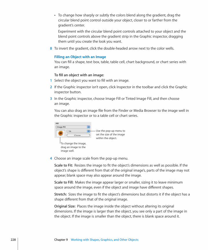
To change how sharply or subtly the colors blend along the gradient, drag the Âcircular blend point control outside your object, closer to or farther from the gradient’s center.
Experiment with the circular blend point controls attached to your object and the blend point controls above the gradient strip in the Graphic inspector, dragging them until you create the look you want.
8 To invert the gradient, click the double-headed arrow next to the color wells.
Filling an Object with an ImageYou can fill a shape, text box, table, table cell, chart background, or chart series with an image.
To fill an object with an image: 1 Select the object you want to fill with an image.
2 If the Graphic inspector isn’t open, click Inspector in the toolbar and click the Graphic inspector button.
3 In the Graphic inspector, choose Image Fill or Tinted Image Fill, and then choose an image.
You can also drag an image file from the Finder or Media Browser to the image well in the Graphic inspector or to a table cell or chart series.
Use the pop-up menu to set the size of the image within the object.
To change the image, drag an image to the image well.
4 Choose an image scale from the pop-up menu.
Scale to Fit:� Resizes the image to fit the object’s dimensions as well as possible. If the object’s shape is different from that of the original image’s, parts of the image may not appear; blank space may also appear around the image.
Scale to Fill:� Makes the image appear larger or smaller, sizing it to leave minimum space around the image, even if the object and image have different shapes.
Stretch:� Sizes the image to fit the object’s dimensions but distorts it if the object has a shape different from that of the original image.
Original Size:� Places the image inside the object without altering its original dimensions. If the image is larger than the object, you see only a part of the image in the object. If the image is smaller than the object, there is blank space around it.
228 Chapter 9 Working with Shapes, Graphics, and Other Objects
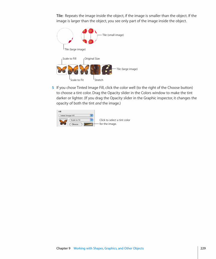
Chapter 9 Working with Shapes, Graphics, and Other Objects 229
Tile:� Repeats the image inside the object, if the image is smaller than the object. If the image is larger than the object, you see only part of the image inside the object.
Tile (small image)
Tile (large image)
Scale to Fit Stretch
Original Size
Tile (large image)
Scale to Fill
5 If you chose Tinted Image Fill, click the color well (to the right of the Choose button) to choose a tint color. Drag the Opacity slider in the Colors window to make the tint darker or lighter. (If you drag the Opacity slider in the Graphic inspector, it changes the opacity of both the tint and the image.)
Click to select a tint color for the image.
Working with MathTypeIf you have MathType 6 installed, you can open it within Numbers and use it to type mathematical expressions and equations. After you’ve created an equation in MathType 6, you can manipulate the equation as an image in Numbers.
To type an equation using MathType 6 within Numbers:� 1 Place the pointer where you want the equation to appear.
2 Choose Insert > MathType Equation.
MathType 6 opens and the equation “E=mc2” appears.
3 Double-click the equation and type the equation you want using the MathType 6 application window and tools.
Refer to MathType 6 Help for specific instructions on how to use this product.
4 When you finish typing your equation, choose File > “Close and Return to Numbers,” and then click Yes in the window that appears to save the equation.
5 Drag the equation wherever you want it on the sheet.
After you close MathType 6, Numbers treats the equation as an object that you can reposition, resize, reorient, group, layer, or even mask like an image. However, if you mask the equation, you must unmask it in order to edit it further.
6 To edit the equation, double-click it to open MathType 6 again.
230 Chapter 9 Working with Shapes, Graphics, and Other Objects
231
This chapter describes how to add contact information stored in Address Book and vCards to a Numbers table.
Address Book fields are a rich source of names, phone numbers, addresses, and other data for people. You can use Address Book data to quickly create tables that consolidate information you need for business contacts, personal friends, holiday correspondents, and so on.
Using Address Book FieldsYou can insert data from Address Book fields into Numbers tables. You can also insert data from a virtual address card (vCard) that someone has sent you.
When a table has a header row containing names that match Address Book or vCard field names, you can add contact data by dragging cards to the table. You can also create a new table by dragging cards to the canvas.
To learn about Go to
The Address Book fields that Numbers supports “Mapping Column Names to Address Book Field Names” on page 231
Adding data from Address Book or a vCard to an existing table
“Adding Address Book Data to an Existing Table” on page 234
Adding data from Address Book or a vCard and creating a table in a single step
“Adding Address Book Data to a New Table” on page 234
Inserting contact and other data from a Numbers table into a Pages document
Pages Help or the Pages ’09 User Guide
Mapping Column Names to Address Book Field NamesThe following table summarizes the Address Book fields that Numbers supports. The synonyms are alternative names you can use to add a particular Address Book field value.
10Adding Address Book Data to a Table
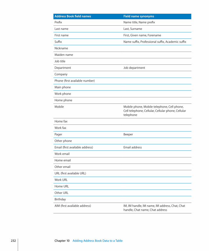
Address Book field names Field name synonyms
Prefix Name title, Name prefix
Last name Last, Surname
First name First, Given name, Forename
Suffix Name suffix, Professional suffix, Academic suffix
Nickname
Maiden name
Job title
Department Job department
Company
Phone (first available number)
Main phone
Work phone
Home phone
Mobile Mobile phone, Mobile telephone, Cell phone, Cell telephone, Cellular, Cellular phone, Cellular telephone
Home fax
Work fax
Pager Beeper
Other phone
Email (first available address) Email address
Work email
Home email
Other email
URL (first available URL)
Work URL
Home URL
Other URL
Birthday
AIM (first available address) IM, IM handle, IM name, IM address, Chat, Chat handle, Chat name, Chat address
232 Chapter 10 Adding Address Book Data to a Table
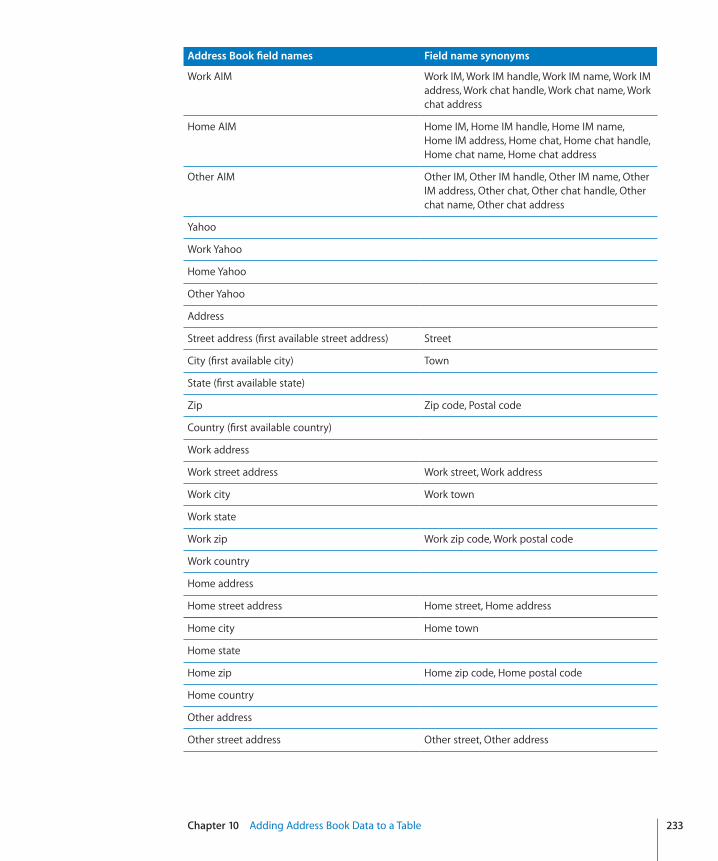
Chapter 10 Adding Address Book Data to a Table 233
Address Book field names Field name synonyms
Work AIM Work IM, Work IM handle, Work IM name, Work IM address, Work chat handle, Work chat name, Work chat address
Home AIM Home IM, Home IM handle, Home IM name, Home IM address, Home chat, Home chat handle, Home chat name, Home chat address
Other AIM Other IM, Other IM handle, Other IM name, Other IM address, Other chat, Other chat handle, Other chat name, Other chat address
Yahoo
Work Yahoo
Home Yahoo
Other Yahoo
Address
Street address (first available street address) Street
City (first available city) Town
State (first available state)
Zip Zip code, Postal code
Country (first available country)
Work address
Work street address Work street, Work address
Work city Work town
Work state
Work zip Work zip code, Work postal code
Work country
Home address
Home street address Home street, Home address
Home city Home town
Home state
Home zip Home zip code, Home postal code
Home country
Other address
Other street address Other street, Other address
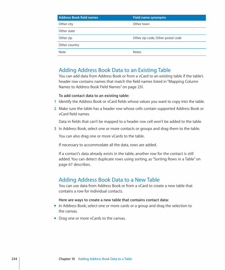
Address Book field names Field name synonyms
Other city Other town
Other state
Other zip Other zip code, Other postal code
Other country
Note Notes
Adding Address Book Data to an Existing TableYou can add data from Address Book or from a vCard to an existing table if the table’s header row contains names that match the field names listed in “Mapping Column Names to Address Book Field Names” on page 231.
To add contact data to an existing table:� 1 Identify the Address Book or vCard fields whose values you want to copy into the table.
2 Make sure the table has a header row whose cells contain supported Address Book or vCard field names.
Data in fields that can’t be mapped to a header row cell won’t be added to the table.
3 In Address Book, select one or more contacts or groups and drag them to the table.
You can also drag one or more vCards to the table.
If necessary to accommodate all the data, rows are added.
If a contact’s data already exists in the table, another row for the contact is still added. You can detect duplicate rows using sorting, as “Sorting Rows in a Table” on page 67 describes.
Adding Address Book Data to a New TableYou can use data from Address Book or from a vCard to create a new table that contains a row for individual contacts.
Here are ways to create a new table that contains contact data:�In Address Book, select one or more cards or a group and drag the selection to m
the canvas.
Drag one or more vCards to the canvas. m
234 Chapter 10 Adding Address Book Data to a Table

Chapter 10 Adding Address Book Data to a Table 235
The table contains a column for each Address Book or vCard field named, as “Mapping Column Names to Address Book Field Names” on page 231 describes. However, only fields named Last name, First name, Phone, and Email are initially visible; the other columns are hidden. To view the hidden columns, choose Table > Unhide All Columns. You can delete or rename columns as required.
236
This chapter describes the various ways you can distribute your Numbers spreadsheet so others can access it.
In addition to printing or faxing your spreadsheet, you can share your spreadsheet electronically. By exporting to other document formats, you can collaborate with others who use Excel and other applications. You can also share spreadsheets on the web and using Mail.
Printing a SpreadsheetYou can use Print View to lay out objects on your sheets across pages before printing. See “Dividing a Sheet into Pages” on page 42 for instructions. Use the Sheets inspector to set up page attributes such as page orientation and margins.
To print:� 1 Choose File > Print.
2 Choose the printer you want to use from the Printer pop-up menu.
3 Type the number of copies you want to print in the Copies field, and then select Collated if you want each group of pages to print together in order before printing the next group. If you want to print a batch of page 1, then page 2, then page 3, and so on, deselect Collated.
4 Indicate which sheets you want to print:
All sheets:� Prints all the sheets in your spreadsheet.
Current Sheet:� Prints only the sheet selected when you opened the print window.
5 To print a list of all formulas in the spreadsheet, select “Include a list of all formulas in the document.”
6 Click Print.
To learn about additional print settings, click the Help button in the print window.
11Sharing Your Numbers Spreadsheet
Chapter 11 Sharing Your Numbers Spreadsheet 237
Exporting a Spreadsheet to Other Document FormatsYou can share your Numbers spreadsheets on different platforms and with various applications by exporting them to a file in PDF, Excel, or comma-separated values (CSV) format.
To learn how to Go to
Create a PDF file of your spreadsheet and optionally password-protect it
“Exporting a Spreadsheet in PDF Format” on page 237
Create a file of your spreadsheet that can be opened and edited in Microsoft Excel on a Mac OS X computer or on a Windows computer
“Exporting a Spreadsheet in Excel Format” on page 238
Create a file of your spreadsheet for applications that can open CSV files
“Exporting a Spreadsheet in CSV Format” on page 238
Exporting a Spreadsheet in PDF FormatPDF files can be viewed or printed in Preview, viewed or printed in Safari, and edited with a PDF application.
To create a PDF file of your spreadsheet: 1 Choose Share > Export.
2 Click PDF.
3 Choose an image resolution from the Image Quality pop-up menu.
Good:� Images are downsampled to 72 dpi.
Better:� Images are downsampled to 150 dpi.
Best:� Images aren’t scaled down.
4 Choose which sheets to export from the Layout pop-up menu.
Sheet View:� Exports each sheet to a single page in the PDF.
Page View:� Exports the selected sheet using the pagination currently configured in Print View. To learn about Print View, see “Dividing a Sheet into Pages” on page 42.
5 Click the Security Options disclosure triangle to password-protect the PDF.
Passwords are limited to 32 ASCII characters. Select one or more of the following options.
Open Document:� Specify a password required to open the PDF.
Print document:� Require a password to print the PDF. If you select this option, also select Open Document and specify a password.
Copy content from the document:� Specify a password required to copy content from the PDF.
6 Click Next to specify a name and location for the PDF.
7 Click Export to create the PDF.
Exporting a Spreadsheet in Excel FormatFiles in Excel format can be opened and edited in Microsoft Excel on a Mac OS X computer or on a Windows computer.
Each table is converted to an Excel worksheet, and all other objects are placed on separate worksheets if there’s more than one table.
Here are ways to create an Excel version of your spreadsheet:�Choose Share > Export, and then click Excel. m
Select Summary if you don’t want a summary worksheet included for multi-worksheet exports. Select Next to specify a name and location for the file, and then click Export to create it.
Choose File > Save As, select “Save copy as,” and choose Excel Document from the m
pop-up menu. See “Saving a Spreadsheet” on page 32 to learn about the other options available when using this approach.
Some of the formula calculations may differ in Excel.
Exporting a Spreadsheet in CSV FormatMany spreadsheet applications can open a file in CSV format. In a CSV file, cell values in each row are separated by commas. Rows are separated by end-of-line characters.
Each table is placed in its own CSV file, and all the files are placed in a folder. No graphics are exported. The last calculated values are exported.
To create a CSV version of your spreadsheet:� 1 Choose Share > Export.
2 Click CSV.
3 Choose an option from the Text Encoding pop-up menu.
Unicode (UTF-8):� This option is supported by almost all applications.
Western (Mac OS Roman) or Western (Windows Latin 1):� These options are for applications that require them.
4 Click Next to specify a file name and location.
5 Click Export to create the file.
238 Chapter 11 Sharing Your Numbers Spreadsheet
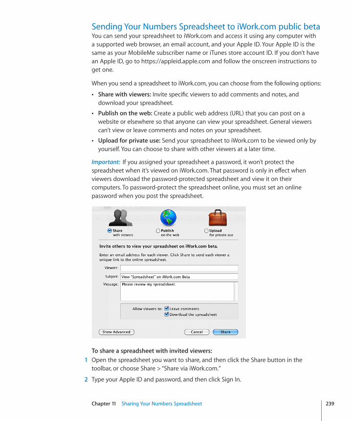
Chapter 11 Sharing Your Numbers Spreadsheet 239
Sending Your Numbers Spreadsheet to iWork.com public betaYou can send your spreadsheet to iWork.com and access it using any computer with a supported web browser, an email account, and your Apple ID. Your Apple ID is the same as your MobileMe subscriber name or iTunes store account ID. If you don’t have an Apple ID, go to https://appleid.apple.com and follow the onscreen instructions to get one.
When you send a spreadsheet to iWork.com, you can choose from the following options:
 Share with viewers:� Invite specific viewers to add comments and notes, and download your spreadsheet.
 Publish on the web:� Create a public web address (URL) that you can post on a website or elsewhere so that anyone can view your spreadsheet. General viewers can’t view or leave comments and notes on your spreadsheet.
 Upload for private use:� Send your spreadsheet to iWork.com to be viewed only by yourself. You can choose to share with other viewers at a later time.
Important: If you assigned your spreadsheet a password, it won’t protect the spreadsheet when it’s viewed on iWork.com. That password is only in effect when viewers download the password-protected spreadsheet and view it on their computers. To password-protect the spreadsheet online, you must set an online password when you post the spreadsheet.
To share a spreadsheet with invited viewers:� 1 Open the spreadsheet you want to share, and then click the Share button in the
toolbar, or choose Share > “Share via iWork.com.”
2 Type your Apple ID and password, and then click Sign In.
If you've forgotten your Apple ID or password, click Forgot Password, and then follow the onscreen instructions.
If it’s your first time sending a document to iWork.com, an email verification is sent to your email address. Click the verification link in the email, and then continue sharing your document.
3 Select “Share with viewers.”
4 In the To and Message fields, type the email addresses and a message for the people you want to allow access to the spreadsheet.
5 Type a subject if you don’t want to use the one created automatically.
6 Set viewing options for your shared spreadsheet. Click Show Advanced to see all of these options:
Leave comments:� Select to allow viewers to leave comments on the spreadsheet.
Download the spreadsheet:� Select to allow viewers to download the spreadsheet.
Copy to iWork.com as:� Type or choose a filename for the online spreadsheet.
Download Options:� Select one or more file format options in which to make the spreadsheet available for download.
Privacy:� Select to require viewers to enter a password before viewing the spreadsheet online. Type an online password in the fields provided, and then click Set Password. Be sure to notify viewers of the spreadsheet’s password.
You can use the Password Assistant (click the button with the key icon) to help you create a stronger password. To learn more about the Password Assistant, see “Password-Protecting a Spreadsheet” on page 31.
7 Click Share.
A copy of your spreadsheet is sent to iWork.com and invitations are emailed to your viewers. Viewers click the unique link in their email to access your spreadsheet online. If they leave comments, their name appears on the comments.
To publish a spreadsheet on the web for general viewing:� 1 Open the spreadsheet you want to share, and then click the Share button in the
toolbar, or choose Share > “Share via iWork.com.”
2 Type your Apple ID and password, and then click Sign In.
If you've forgotten your Apple ID or password, click Forgot Password, and then follow the onscreen instructions.
If it’s your first time sending a document to iWork.com, an email verification is sent to your email address. Click the verification link in the email, and then continue publishing your document.
3 Select “Publish on the web.”
240 Chapter 11 Sharing Your Numbers Spreadsheet
Chapter 11 Sharing Your Numbers Spreadsheet 241
4 Click Show Advanced if you want to change the online name of the spreadsheet, and then type or choose a filename for the online document.
5 Click Publish.
A copy of your spreadsheet is published to iWork.com. Viewers can view your spreadsheet, but they can’t add comments and notes to it.
6 In the dialog that appears, click View Online to see your spreadsheet on iWork.com.
Your browser opens and displays the published spreadsheet on iWork.com.
7 In your browser window, click Show Public URL to see the web address for your document.
You can copy the web address (URL) and post it on a website or elsewhere. Anyone with the web address can view your spreadsheet online.
To upload a spreadsheet for your private access:� 1 Open the spreadsheet, and then click the Share button in the toolbar, or choose
Share > “Share via iWork.com.”
2 Type your Apple ID and password, and then click Sign In.
If you've forgotten your Apple ID or password, click Forgot Password, and then follow the onscreen instructions.
If it’s your first time sending a document to iWork.com, an email verification is sent to your email address. Click the verification link in the email, and then continue uploading your document.
3 Select “Upload for private use.”
4 Click Show Advanced if you want to change the online name of the spreadsheet, and then type or choose a filename for the online spreadsheet.
5 Click the Upload button
A copy of your spreadsheet is sent to iWork.com.
6 Click View Online to see your spreadsheet on iWork.com, or click OK to close the dialog.
To access all your online spreadsheets from the Shared Documents view of iWork.com, do either of the following:�Open a spreadsheet and choose Share > Show Shared Documents. If you’re not m
already logged in, choose Share > Sign In, and then choose Show Shared Documents.
Go to m http://www.iwork.com/ and sign in.
You can set iWork.com to notify you by email when viewers post new comments to an online spreadsheet. For this information and more details about using iWork.com, go to http://www.iwork.com/ and click Help at the bottom of the page.
Sending a Spreadsheet Using EmailAttach your spreadsheet in Numbers, Excel, or PDF format to an email message. If you password-protected the spreadsheet, the password settings are retained for Numbers attachments.
To attach a spreadsheet to an email message:� 1 If you want to email a spreadsheet in Numbers format, you can password-protect it first.
See “Password-Protecting a Spreadsheet” on page 31 to learn how to password-protect a spreadsheet.
2 Choose Share > “Send via Mail” and then choose Numbers, Excel, or PDF from the submenu.
A new email message opens in your default mail application, with a Numbers, Excel, or PDF version of your spreadsheet attached.
Sending a Spreadsheet to iWebIf you use (or intend to use) iWeb to create a website, you can send a Numbers spreadsheet directly to your iWeb blog or podcast. The spreadsheet becomes an attachment that your website visitors can download.
To send a spreadsheet to iWeb:� 1 Make sure you have iWeb ’08 or later installed.
2 Open your Numbers spreadsheet, and then choose Share > “Send to iWeb” and then choose Numbers or PDF from the submenu.
Numbers:� Creates an archive version of your spreadsheet. If the spreadsheet is password-protected, the password settings are retained.
PDF:� Creates a PDF version.
3 If iWeb wasn’t open, it opens, and you can choose a new or existing blog or podcast to attach your spreadsheet to. If you have only one blog or podcast, the spreadsheet is attached to it.
When you publish your website, visitors who subscribe to your blog or podcast automatically get the latest attachments sent to their iTunes library (PDF publish only).
For more information about using iWeb to design and publish webpages, open iWeb and choose Help > iWeb Help.
242 Chapter 11 Sharing Your Numbers Spreadsheet
Chapter 11 Sharing Your Numbers Spreadsheet 243
Sharing Charts, Data, and Tables with other iWork ApplicationsYou can copy a chart and paste it into a Keynote presentation or a Pages document. After it’s pasted, the chart is linked to the Numbers version. If the Numbers table data depicted in the chart changes, save the changed Numbers spreadsheet and then refresh the chart in Keynote or Pages. See “Sharing Charts with Pages and Keynote Documents” on page 143 for more information.
Pages documents can take advantage of Address Book, vCard, and other data stored in Numbers tables. See “Using Address Book Fields” on page 231 to learn about using Address Book and vCard data in Numbers. See Pages Help or the Pages ’09 User Guide to learn how to use Numbers data for mail merge.
You can copy a table to Pages or Keynote documents. See “Copying Tables Among iWork Applications” on page 54 for more information.
244
This chapter is for designers who want to create their own spreadsheet templates.
This chapter assumes you are already familiar with the features of Numbers described in earlier chapters.
Designing a TemplateThe templates that come with Numbers provide ideas for designing the look of charts, tables, and other objects.
To create your own templates, you can do something as simple as adding your company logo to an existing template. Or you can modify these attributes of a Numbers template:
Table styles Â
Reusable tables available when you click Tables in the toolbar Â
Default formatting for different types of charts Â
Default attributes of text boxes, shapes, and images Â
The number and names of sheets Â
Predefined content on sheets, such as text, tables, and media placeholders Â
To learn how to Go to
Set up a template’s table styles “Defining Table Styles for a Custom Template” on page 245
Create predefined tables to provide in the template
“Defining Reusable Tables for a Custom Template” on page 245
Set up charts and other objects for the template “Defining Default Charts, Text Boxes, Shapes, and Images for a Custom Template” on page 245
Create initial content “Creating Initial Spreadsheet Content for a Custom Template” on page 247
Save your template “Saving a Custom Template” on page 249
12Designing Your Own Numbers Spreadsheet Templates
Chapter 12 Designing Your Own Numbers Spreadsheet Templates 245
Defining Table Styles for a Custom TemplateA template has one or more table styles that let you format a selected table in a single click. Table styles are useful for applying consistent formatting to tables.
You can use or redefine the table styles in a Numbers template, or you can create your own styles. See “Using Table Styles” on page 114 to learn how.
Defining Reusable Tables for a Custom TemplateA template has one or more reusable tables, which let you add tables that have already been styled and sized. They can also contain predefined content, such as formulas and text.
When using a template, you add a reusable table by clicking Tables in the toolbar and choosing a table from the pop-up menu.
You can use or redefine the reusable tables in a Numbers template, or you can create your own. “Defining Reusable Tables” on page 53 provides instructions.
Defining Default Charts, Text Boxes, Shapes, and Images for a Custom TemplateA template has default values defined for the following objects, which take effect when a template user adds one of them:
Charts Â
Text boxes Â
Shapes Â
Imported images Â
You can use the default settings that already exist in the template you started with, or you can change the settings.
To learn how to Go to
Set up default chart attributes “Defining Default Attributes for Charts” on page 245
Set up default attributes for text boxes and shapes
“Defining Default Attributes for Text Boxes and Shapes” on page 246
Set up default image attributes “Defining Default Attributes for Imported Images” on page 246
Defining Default Attributes for ChartsYou can set the default appearance of each chart type. Default attributes must be set individually for each chart type.
To set default chart attributes:� 1 Place a chart on the sheet by clicking Charts in the toolbar and choosing a chart type.
2 Select the chart, and then set its attributes.
To resize a chart, rotate it, and set other attributes that charts have in common, see “Formatting Charts” on page 143.
To learn how to format pie charts, bar charts, and other specific chart types, see “Formatting Specific Chart Types” on page 154.
3 Repeat steps 1 and 2 for each chart type for which you want to define default attributes.
4 Select a chart, and then choose Format > Advanced > Define Default Style for chart type.
Repeat this action for each chart you’re setting up.
5 Delete the charts from the spreadsheet.
Defining Default Attributes for Text Boxes and ShapesThe default attributes of text boxes and shapes determine their fill, stroke, shadow, and opacity when they’re first inserted on a sheet. Default attributes also determine the appearance of text you place in the boxes or shapes.
To define default text boxes and shapes: 1 Add the objects to a sheet.
Click Text Box in the toolbar to add a text box, and click Shapes in the toolbar and choose any shape.
2 To set up attributes for text within the text box or shape, select the object, add text to it, then format the text attributes.
See “Formatting Text Size and Appearance” on page 165 for instructions.
3 To set up object attributes, select the text box or shape and then follow the instructions in “Manipulating, Arranging, and Changing the Look of Objects” on page 212.
4 Save the text box and shape as default objects.
To save the text box, select it and then choose Format > Advanced > Define Default Text Box Style.
To save the shape, select it and then choose Format > Advanced > Define Default shape Style.
5 Delete the text box and shape from the sheet.
Defining Default Attributes for Imported ImagesFor imported graphics, you can set default shadows, opacity, borders, and more.
246 Chapter 12 Designing Your Own Numbers Spreadsheet Templates
Chapter 12 Designing Your Own Numbers Spreadsheet Templates 247
To set default image attributes:� 1 Import an image, as “Working with Images” on page 194 describes.
2 Select the image, and then set its attributes.
To remove unwanted parts of an image, see “Masking (Cropping) Images” on page 196 and “Removing the Background or Unwanted Elements from an Image” on page 198.
To improve the image quality and create interesting effects, see “Changing an Image’s Brightness, Contrast, and Other Settings” on page 199.
To place and reformat the image, see “Manipulating, Arranging, and Changing the Look of Objects” on page 212.
3 Choose Format > Advanced > Define Default Image Style.
4 Delete the image from the sheet.
Creating Initial Spreadsheet Content for a Custom TemplateYou can use predefined content to model the look of a finished spreadsheet or to provide instructions and other productivity aids for template users.
To learn how to Go to
Add names, formulas, and other content “Predefining Tables and Other Objects for a Custom Template” on page 247
Define a media placeholder “Creating Media Placeholders for a Custom Template” on page 248
Organize content into sheets “Predefining Sheets for a Custom Template” on page 248
Predefining Tables and Other Objects for a Custom TemplateAdd tables, charts, text boxes, images, shapes, and other initial content to your templates to help users be more productive and to make the objects in the spreadsheet visually appealing.
For example, you can:
Add names to tables and titles to charts and their axes Â
Add formulas and other predefined content to table cells Â
Set up cells so their values are displayed in particular ways (for example, using a Ânumber format or checkboxes)
Create text boxes or comments that provide instructions and suggestions for using Âthe template
Use color to heighten the prominence of particular elements in tables and charts Â
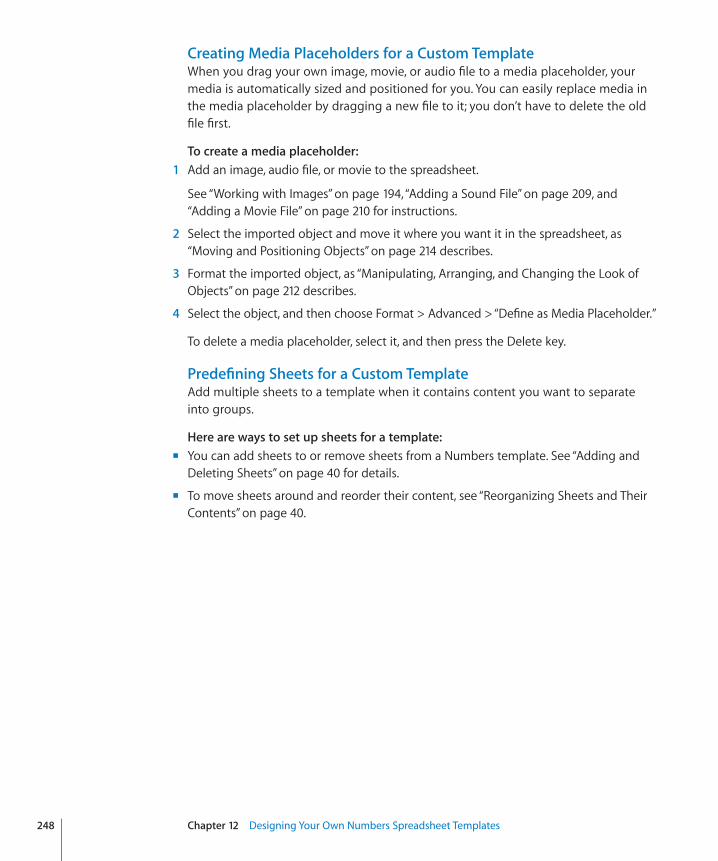
Creating Media Placeholders for a Custom TemplateWhen you drag your own image, movie, or audio file to a media placeholder, your media is automatically sized and positioned for you. You can easily replace media in the media placeholder by dragging a new file to it; you don’t have to delete the old file first.
To create a media placeholder:� 1 Add an image, audio file, or movie to the spreadsheet.
See “Working with Images” on page 194, “Adding a Sound File” on page 209, and “Adding a Movie File” on page 210 for instructions.
2 Select the imported object and move it where you want it in the spreadsheet, as “Moving and Positioning Objects” on page 214 describes.
3 Format the imported object, as “Manipulating, Arranging, and Changing the Look of Objects” on page 212 describes.
4 Select the object, and then choose Format > Advanced > “Define as Media Placeholder.”
To delete a media placeholder, select it, and then press the Delete key.
Predefining Sheets for a Custom TemplateAdd multiple sheets to a template when it contains content you want to separate into groups.
Here are ways to set up sheets for a template:�You can add sheets to or remove sheets from a Numbers template. See “ m Adding and Deleting Sheets” on page 40 for details.
To move sheets around and reorder their content, see “ m Reorganizing Sheets and Their Contents” on page 40.
248 Chapter 12 Designing Your Own Numbers Spreadsheet Templates
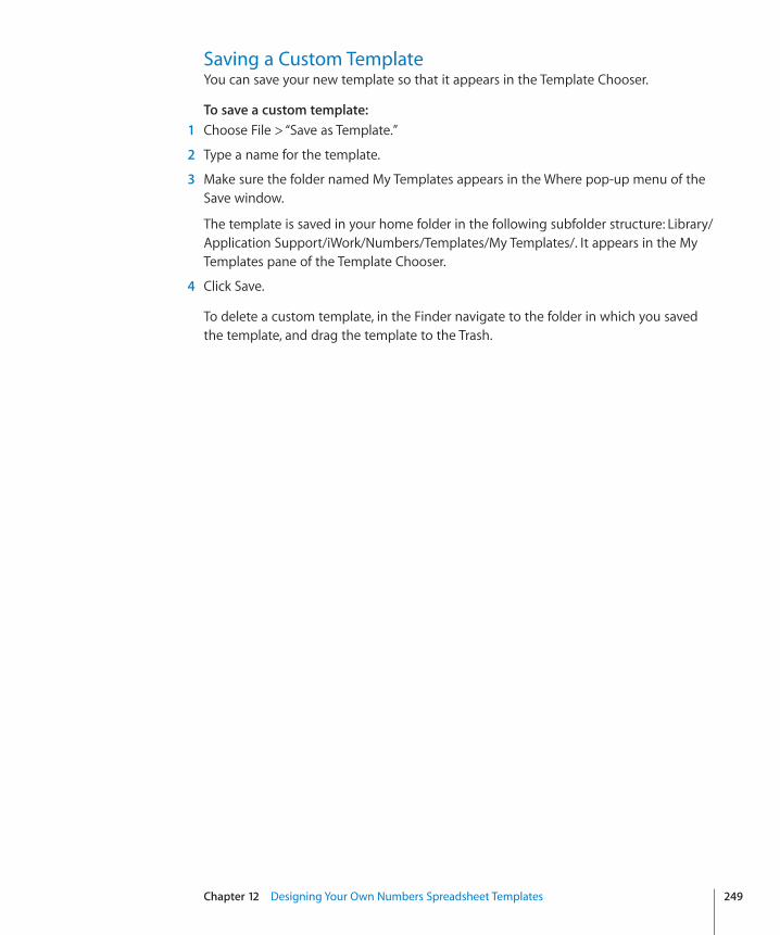
Chapter 12 Designing Your Own Numbers Spreadsheet Templates 249
Saving a Custom TemplateYou can save your new template so that it appears in the Template Chooser.
To save a custom template:� 1 Choose File > “Save as Template.”
2 Type a name for the template.
3 Make sure the folder named My Templates appears in the Where pop-up menu of the Save window.
The template is saved in your home folder in the following subfolder structure: Library/Application Support/iWork/Numbers/Templates/My Templates/. It appears in the My Templates pane of the Template Chooser.
4 Click Save.
To delete a custom template, in the Finder navigate to the folder in which you saved the template, and drag the template to the Trash.
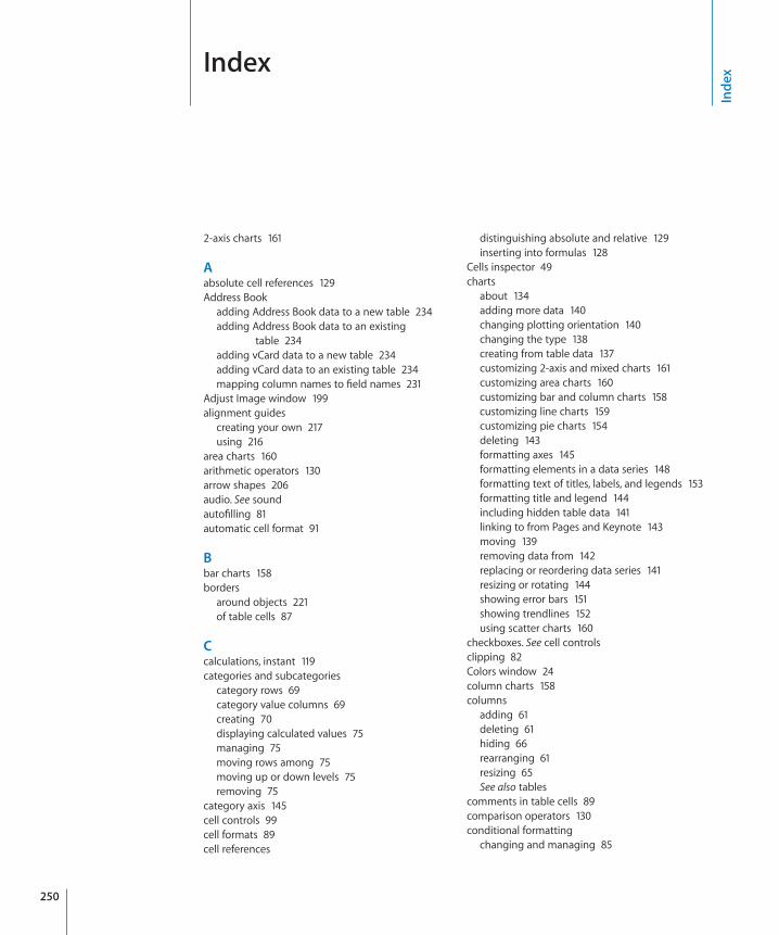
2-axis charts 161
Aabsolute cell references 129Address Book
adding Address Book data to a new table 234adding Address Book data to an existing
table 234adding vCard data to a new table 234adding vCard data to an existing table 234mapping column names to field names 231
Adjust Image window 199alignment guides
creating your own 217using 216
area charts 160arithmetic operators 130arrow shapes 206audio. See soundautofilling 81automatic cell format 91
Bbar charts 158borders
around objects 221of table cells 87
Ccalculations, instant 119categories and subcategories
category rows 69category value columns 69creating 70displaying calculated values 75managing 75moving rows among 75moving up or down levels 75removing 75
category axis 145cell controls 99cell formats 89cell references
distinguishing absolute and relative 129inserting into formulas 128
Cells inspector 49charts
about 134adding more data 140changing plotting orientation 140changing the type 138creating from table data 137customizing 2-axis and mixed charts 161customizing area charts 160customizing bar and column charts 158customizing line charts 159customizing pie charts 154deleting 143formatting axes 145formatting elements in a data series 148formatting text of titles, labels, and legends 153formatting title and legend 144including hidden table data 141linking to from Pages and Keynote 143moving 139removing data from 142replacing or reordering data series 141resizing or rotating 144showing error bars 151showing trendlines 152using scatter charts 160
checkboxes. See cell controlsclipping 82Colors window 24column charts 158columns
adding 61deleting 61hiding 66rearranging 61resizing 65See also tables
comments in table cells 89comparison operators 130conditional formatting
changing and managing 85
Index
250
Inde
x
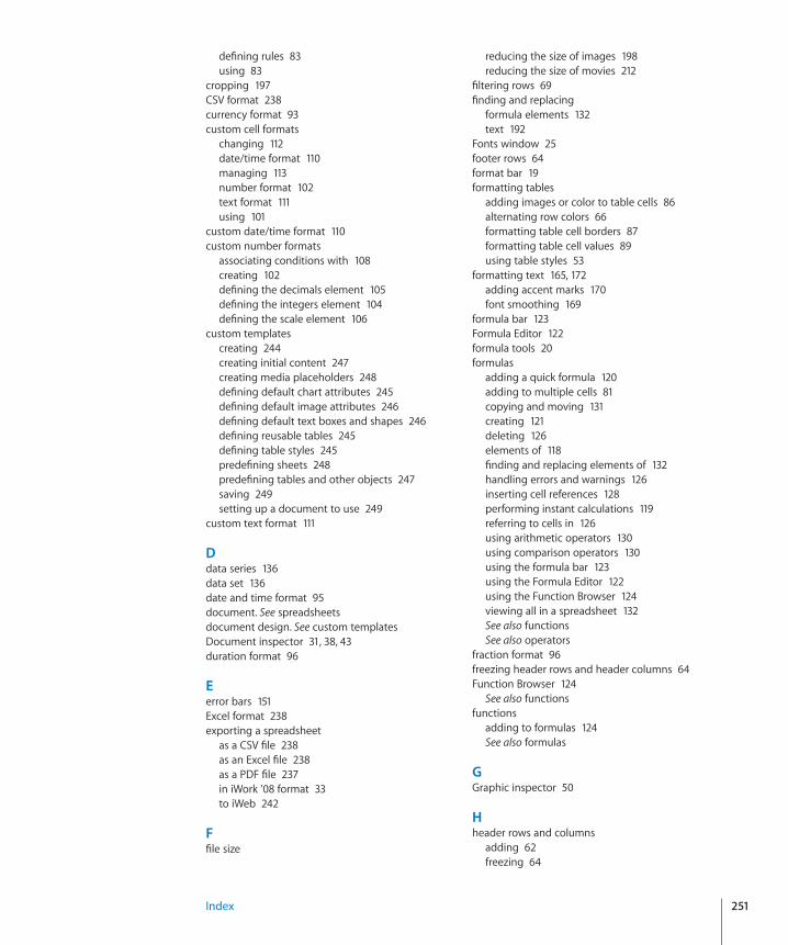
Index 251
defining rules 83using 83
cropping 197CSV format 238currency format 93custom cell formats
changing 112date/time format 110managing 113number format 102text format 111using 101
custom date/time format 110custom number formats
associating conditions with 108creating 102defining the decimals element 105defining the integers element 104defining the scale element 106
custom templatescreating 244creating initial content 247creating media placeholders 248defining default chart attributes 245defining default image attributes 246defining default text boxes and shapes 246defining reusable tables 245defining table styles 245predefining sheets 248predefining tables and other objects 247saving 249setting up a document to use 249
custom text format 111
Ddata series 136data set 136date and time format 95document. See spreadsheetsdocument design. See custom templatesDocument inspector 31, 38, 43duration format 96
Eerror bars 151Excel format 238exporting a spreadsheet
as a CSV file 238as an Excel file 238as a PDF file 237in iWork ’08 format 33to iWeb 242
Ffile size
reducing the size of images 198reducing the size of movies 212
filtering rows 69finding and replacing
formula elements 132text 192
Fonts window 25footer rows 64format bar 19formatting tables
adding images or color to table cells 86alternating row colors 66formatting table cell borders 87formatting table cell values 89using table styles 53
formatting text 165, 172adding accent marks 170font smoothing 169
formula bar 123Formula Editor 122formula tools 20formulas
adding a quick formula 120adding to multiple cells 81copying and moving 131creating 121deleting 126elements of 118finding and replacing elements of 132handling errors and warnings 126inserting cell references 128performing instant calculations 119referring to cells in 126using arithmetic operators 130using comparison operators 130using the formula bar 123using the Formula Editor 122using the Function Browser 124viewing all in a spreadsheet 132See also functionsSee also operators
fraction format 96freezing header rows and header columns 64Function Browser 124
See also functionsfunctions
adding to formulas 124See also formulas
GGraphic inspector 50
Hheader rows and columns
adding 62freezing 64
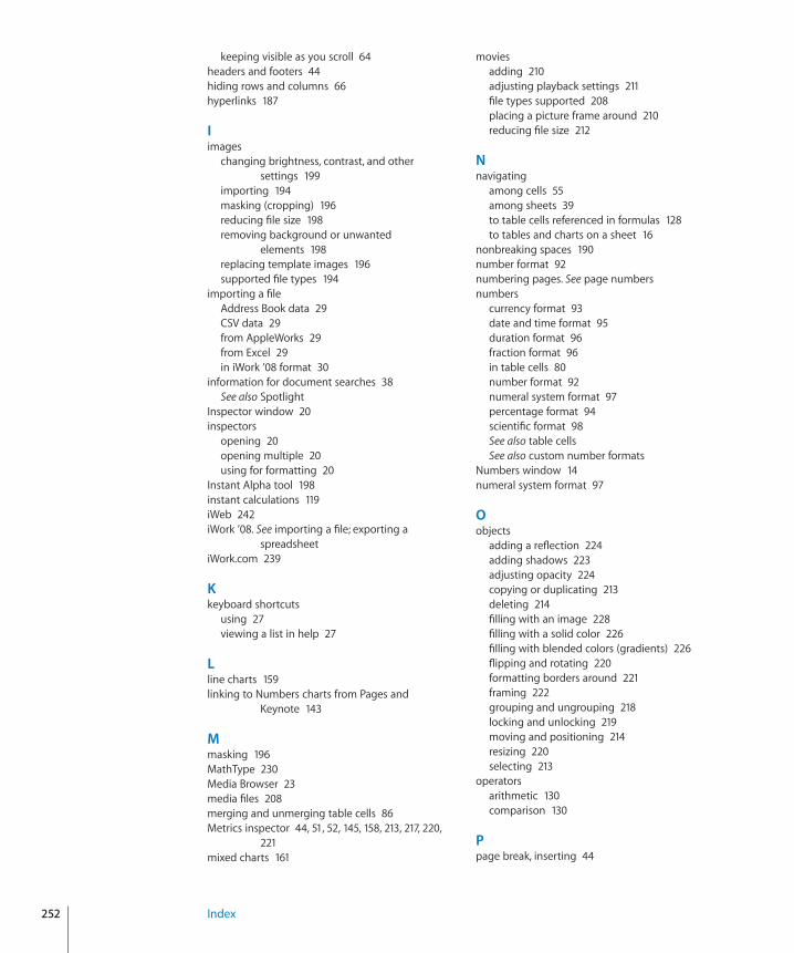
252 Index
keeping visible as you scroll 64headers and footers 44hiding rows and columns 66hyperlinks 187
Iimages
changing brightness, contrast, and other settings 199
importing 194masking (cropping) 196reducing file size 198removing background or unwanted
elements 198replacing template images 196supported file types 194
importing a fileAddress Book data 29CSV data 29from AppleWorks 29from Excel 29in iWork ’08 format 30
information for document searches 38See also Spotlight
Inspector window 20inspectors
opening 20opening multiple 20using for formatting 20
Instant Alpha tool 198instant calculations 119iWeb 242iWork ’08. See importing a file; exporting a
spreadsheetiWork.com 239
Kkeyboard shortcuts
using 27viewing a list in help 27
Lline charts 159linking to Numbers charts from Pages and
Keynote 143
Mmasking 196MathType 230Media Browser 23media files 208merging and unmerging table cells 86Metrics inspector 44, 51, 52, 145, 158, 213, 217, 220,
221mixed charts 161
moviesadding 210adjusting playback settings 211file types supported 208placing a picture frame around 210reducing file size 212
Nnavigating
among cells 55among sheets 39to table cells referenced in formulas 128to tables and charts on a sheet 16
nonbreaking spaces 190number format 92numbering pages. See page numbersnumbers
currency format 93date and time format 95duration format 96fraction format 96in table cells 80number format 92numeral system format 97percentage format 94scientific format 98See also table cellsSee also custom number formats
Numbers window 14numeral system format 97
Oobjects
adding a reflection 224adding shadows 223adjusting opacity 224copying or duplicating 213deleting 214filling with an image 228filling with a solid color 226filling with blended colors (gradients) 226flipping and rotating 220formatting borders around 221framing 222grouping and ungrouping 218locking and unlocking 219moving and positioning 214resizing 220selecting 213
operatorsarithmetic 130comparison 130
Ppage break, inserting 44
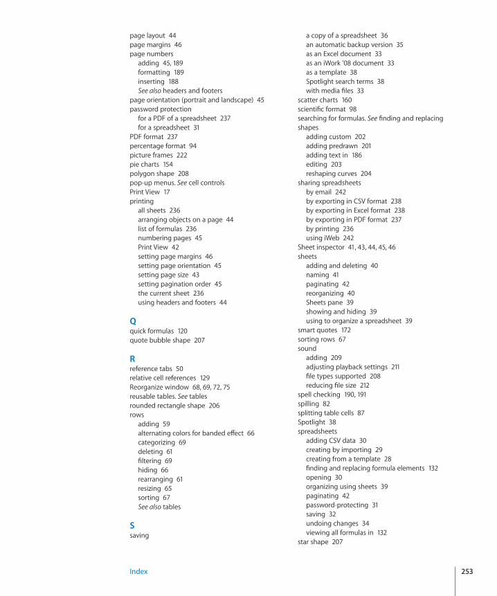
Index 253
page layout 44page margins 46page numbers
adding 45, 189formatting 189inserting 188See also headers and footers
page orientation (portrait and landscape) 45password protection
for a PDF of a spreadsheet 237for a spreadsheet 31
PDF format 237percentage format 94picture frames 222pie charts 154polygon shape 208pop-up menus. See cell controlsPrint View 17printing
all sheets 236arranging objects on a page 44list of formulas 236numbering pages 45Print View 42setting page margins 46setting page orientation 45setting page size 43setting pagination order 45the current sheet 236using headers and footers 44
Qquick formulas 120quote bubble shape 207
Rreference tabs 50relative cell references 129Reorganize window 68, 69, 72, 75reusable tables. See tablesrounded rectangle shape 206rows
adding 59alternating colors for banded effect 66categorizing 69deleting 61filtering 69hiding 66rearranging 61resizing 65sorting 67See also tables
Ssaving
a copy of a spreadsheet 36an automatic backup version 35as an Excel document 33as an iWork ’08 document 33as a template 38Spotlight search terms 38with media files 33
scatter charts 160scientific format 98searching for formulas. See finding and replacingshapes
adding custom 202adding predrawn 201adding text in 186editing 203reshaping curves 204
sharing spreadsheetsby email 242by exporting in CSV format 238by exporting in Excel format 238by exporting in PDF format 237by printing 236using iWeb 242
Sheet inspector 41, 43, 44, 45, 46sheets
adding and deleting 40naming 41paginating 42reorganizing 40Sheets pane 39showing and hiding 39using to organize a spreadsheet 39
smart quotes 172sorting rows 67sound
adding 209adjusting playback settings 211file types supported 208reducing file size 212
spell checking 190, 191spilling 82splitting table cells 87Spotlight 38spreadsheets
adding CSV data 30creating by importing 29creating from a template 28finding and replacing formula elements 132opening 30organizing using sheets 39paginating 42password-protecting 31saving 32undoing changes 34viewing all formulas in 132
star shape 207
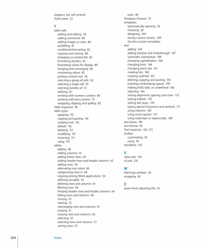
254 Index
steppers. See cell controlsStyles pane 22
Ttable cells
adding and editing 78adding comments 89adding images or color 86autofilling 81conditional formatting 82copying and moving 88enlarging so content fits 82formatting borders 87formatting values for display 89merging and unmerging 86monitoring values 82putting content into 78selecting a group of cells 56selecting a single cell 55selecting borders of 57splitting 87working with numeric content 80working with text content 79wrapping, clipping, and spilling 82
Table inspector 49table styles
applying 115copying and pasting 116creating new 116default 116deleting 117modifying 115renaming 117using 114
tablesadding 48adding columns 61adding footer rows 64adding header rows and header columns 62adding rows 59alternating row colors 66categorizing rows in 69copying among iWork applications 54defining reusable 53deleting rows and columns 61filtering rows 69freezing header rows and header columns 64hiding rows and columns 66moving 52naming 52rearranging rows and columns 61resizing 51resizing rows and columns 65selecting 55selecting rows and columns 57sorting rows 67
tools 48Template Chooser 13templates
automatically opening 29choosing 28designing 244saving custom version 249See also custom templates
textadding 164adding shadow and strikethrough 167automatic substitution 189changing capitalization 168changing fonts 168changing point size 167creating lists 180creating outlined 167deleting, copying, and pasting 165inserting nonbreaking spaces 190making bold, italic, or underlined 166selecting 164setting alignment, spacing, and color 172setting indents 179setting tab stops 178typing special characters and symbols 171using columns 185using smart quotes 172using subscripts or superscripts 168
text boxes 185text format 99Text inspector 165, 172toolbar
customizing 18using 18
trendlines 152
Vvalue axis 145vCards 231
WWarnings window 26wrapping 82
Zzoom level, adjusting the 16


![DATEX II V2.3 USER S GUIDE · [XML schema] DATEX II v2.3 schema 2.3 30-09-2014 Supporting documentation [User guide] DATEX II User’s guide 2.3 30-09-2014 [Software developers guide]](https://img.pdfslide.net/doc/110x75/60c5da18662b2664286eff84/datex-ii-v23-user-s-guide-xml-schema-datex-ii-v23-schema-23-30-09-2014-supporting.jpg)