Numerical Methods

Marisa Villano, Tom Fagan, Dave Fairburn, Chris Savino, David Goldberg, Daniel Rave

An Overview

The Method of Finite Differences Error Approximations and Dangers Approxmations to Diffusions Crank Nicholson Scheme Stability Criterion

Finite Differences

Best known numerical method of approximation

Marisa Villano

Finite Differences

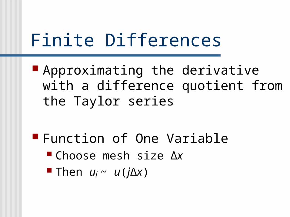
Approximating the derivative with a difference quotient from the Taylor series

Function of One Variable Choose mesh size Δx Then uj ~ u(jΔx)

First Derivative Approximations

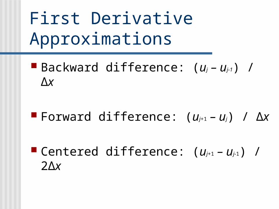
Backward difference: (uj – uj-1) / Δx

Forward difference: (uj+1 – uj) / Δx

Centered difference: (uj+1 – uj-1) / 2Δx

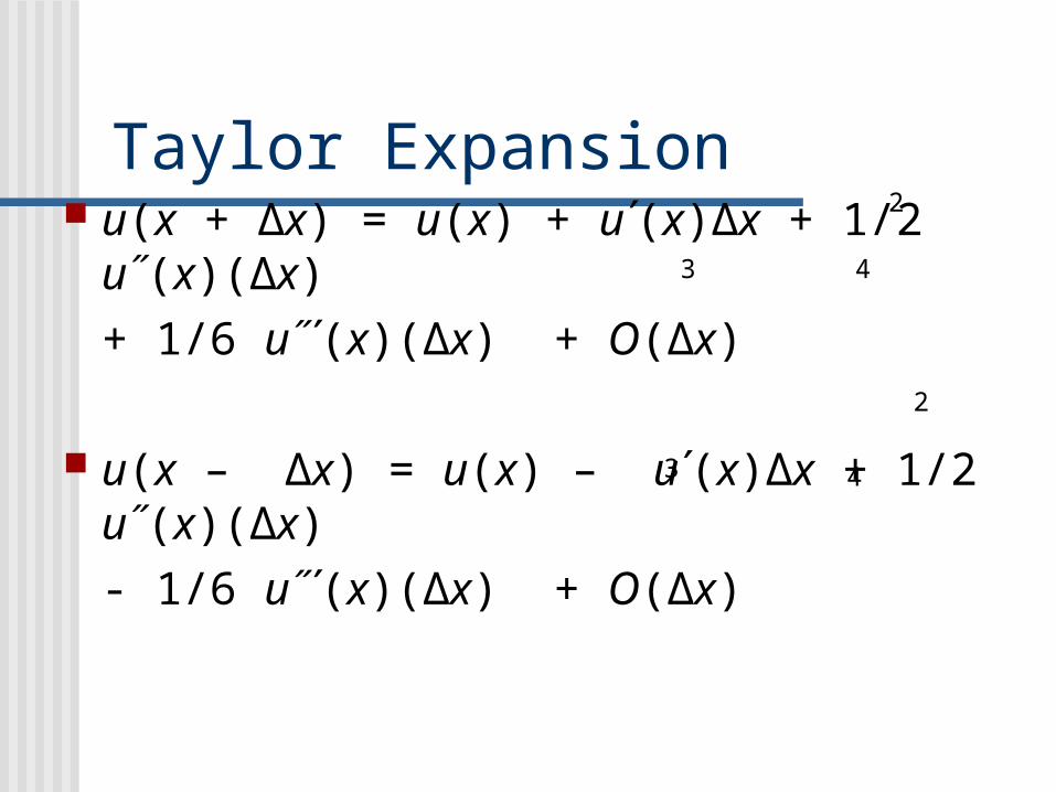
Taylor Expansion u(x + Δx) = u(x) + u΄(x)Δx + 1/2 u˝(x)(Δx)

+ 1/6 u˝΄(x)(Δx) + O(Δx)

u(x – Δx) = u(x) – u΄(x)Δx + 1/2 u˝(x)(Δx)

- 1/6 u˝΄(x)(Δx) + O(Δx)

2

3

4

4

2

3

Taylor Expansion

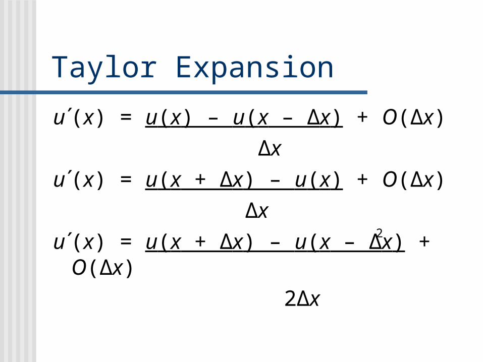
u΄(x) = u(x) – u(x – Δx) + O(Δx)

Δx

u΄(x) = u(x + Δx) – u(x) + O(Δx)

Δx

u΄(x) = u(x + Δx) – u(x – Δx) + O(Δx)

2Δx

2

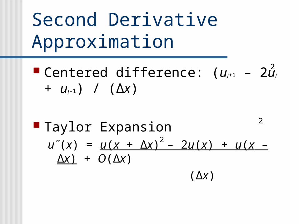
Second Derivative Approximation

Centered difference: (uj+1 – 2uj + uj-1) / (Δx)

Taylor Expansionu˝(x) = u(x + Δx) – 2u(x) + u(x – Δx) + O(Δx)

(Δx)

2

2

2

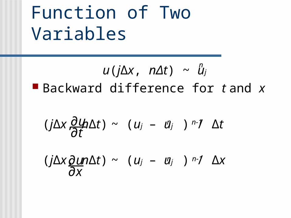
Function of Two Variables

u(jΔx, nΔt) ~ uj Backward difference for t and x

(jΔx, nΔt) ~ (uj – uj ) / Δt

(jΔx, nΔt) ~ (uj – uj ) / Δx

n

n n-1

n-1

n

∂u ∂t

∂u ∂x

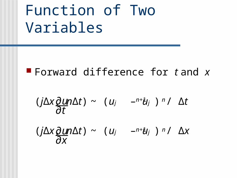
Function of Two Variables

Forward difference for t and x

(jΔx, nΔt) ~ (uj – uj ) / Δt

(jΔx, nΔt) ~ (uj – uj ) / Δx

n+1

n+1 n

n∂u ∂t

∂u ∂x

Function of Two Variables

Centered difference for t and x

(jΔx, nΔt) ~ (uj – uj ) / (2Δt)

(jΔx, nΔt) ~ (uj – uj ) / (2Δx)

n+1

n+1 n-1

n-1∂u ∂t

∂u ∂x

Error Truncation Error: introduced in the solution by the

approximation of the derivative Local Error: from each term of the equation Global Error: from the accumulation of local

error

Roundoff Error: introduced in the computation by the finite number of digits used by the computer

The Dangers of the Finite Difference Method

Evidence from an example in 8.1

Dave Fairburn

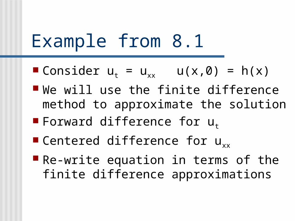
Example from 8.1

Consider ut = uxx u(x,0) = h(x) We will use the finite difference method to

approximate the solution Forward difference for ut

Centered difference for uxx

Re-write equation in terms of the finite difference approximations

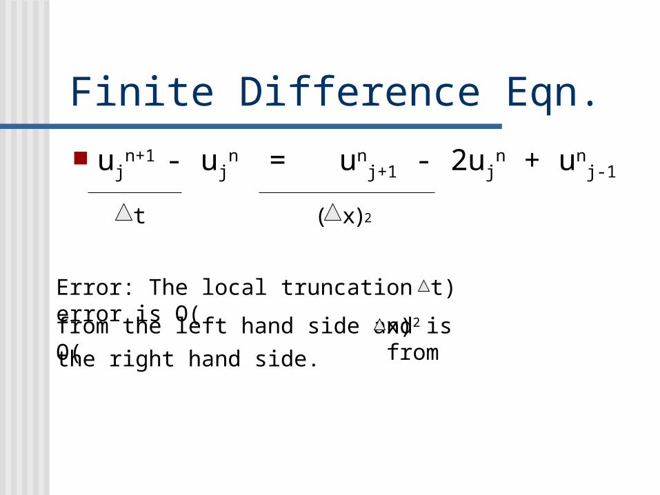
Finite Difference Eqn.

ujn+1 - uj

n = unj+1 - 2uj

n + unj-1

t x( ) 2

Error: The local truncation error is O( t)

from the left hand side and is O( x)2 from

the right hand side.

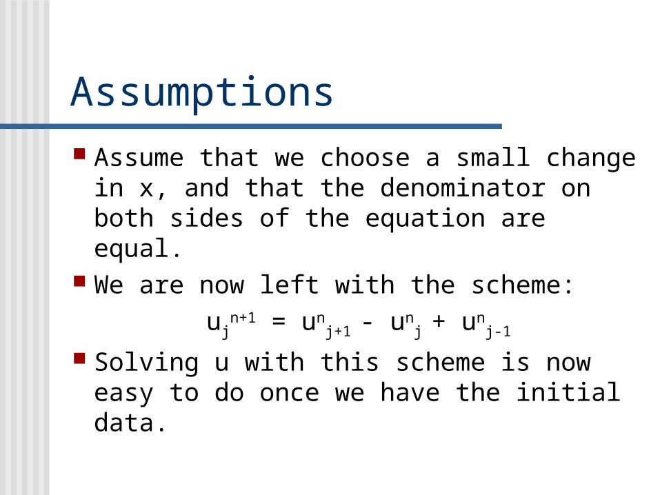
Assumptions

Assume that we choose a small change in x, and that the denominator on both sides of the equation are equal.

We are now left with the scheme:

ujn+1 = un

j+1 - unj + un

j-1

Solving u with this scheme is now easy to do once we have the initial data.

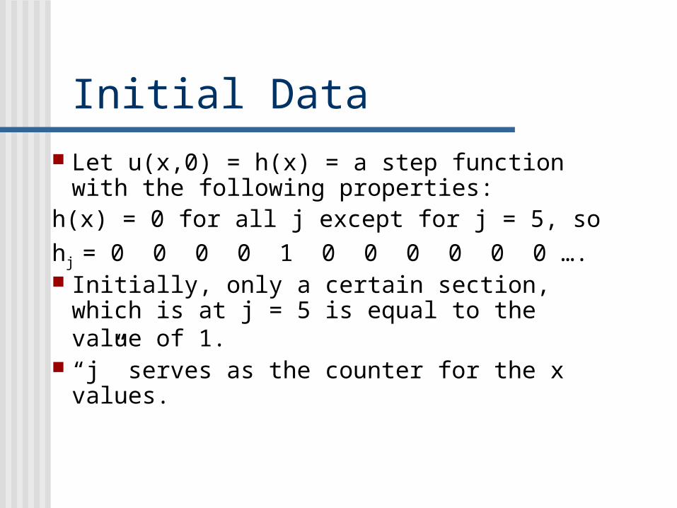
Initial Data

Let u(x,0) = h(x) = a step function with the following properties:

h(x) = 0 for all j except for j = 5, so

hj = 0 0 0 0 1 0 0 0 0 0 0 …. Initially, only a certain section, which is

at j = 5 is equal to the value of 1.

“j” serves as the counter for the x values.

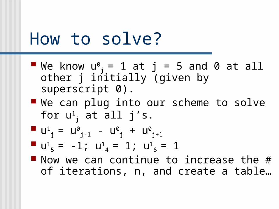
How to solve? We know u0

j = 1 at j = 5 and 0 at all other j initially (given by superscript 0).

We can plug into our scheme to solve for u1j at

all j’s. u1

j = u0j-1 - u0

j + u0j+1

u15 = -1; u1

4 = 1; u16 = 1

Now we can continue to increase the # of iterations, n, and create a table…

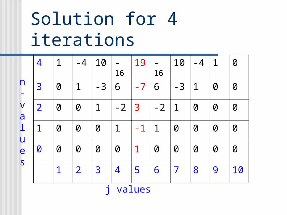
Solution for 4 iterations4 1 -4 10 -16 19 -16 10 -4 1 0

3 0 1 -3 6 -7 6 -3 1 0 0

2 0 0 1 -2 3 -2 1 0 0 0

1 0 0 0 1 -1 1 0 0 0 0

0 0 0 0 0 1 0 0 0 0 0

1 2 3 4 5 6 7 8 9 10

j values

n-values

Analysis of Solution Is this solution viable? Maximum principle states that the solution must

be between 0 and 1 given our initial data At n = 4, our solution has already ballooned to u

= 19! Clearly, there are cases when the finite

difference method can pose serious problems.

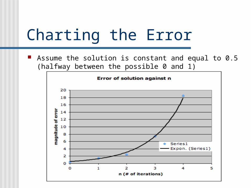
Charting the Error Assume the solution is constant and equal to 0.5 (halfway between

the possible 0 and 1)

Lessons Learned

While the finite difference method is easy and convenient to use in many cases, there are some dangers associated with the method.

We will investigate why the assumption that allowed us to simplify the scheme could have been a major contributor to the large error.

Approximations of Diffusions

Neumann Boundary Conditions and the Crank-Nicolson Scheme

Chris Savino

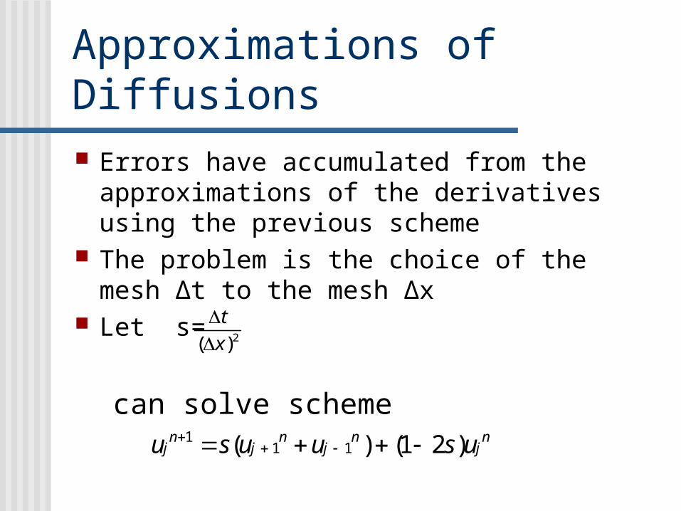
Approximations of Diffusions Errors have accumulated from the

approximations of the derivatives using the previous scheme

The problem is the choice of the mesh Δt to the mesh Δx

Let s=

can solve scheme

2( )

t

x

11 1( ) (1 2 )n n n n

j j j ju s u u s u

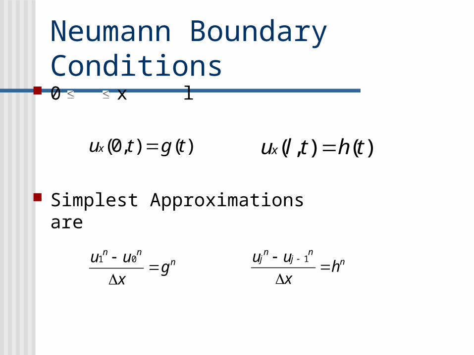
Neumann Boundary Conditions 0 x l

Simplest Approximations are

(0, ) ( )xu t g t ( , ) ( )xu l t h t

1 0n n

nu ug

x

1

n nj j nu u

hx

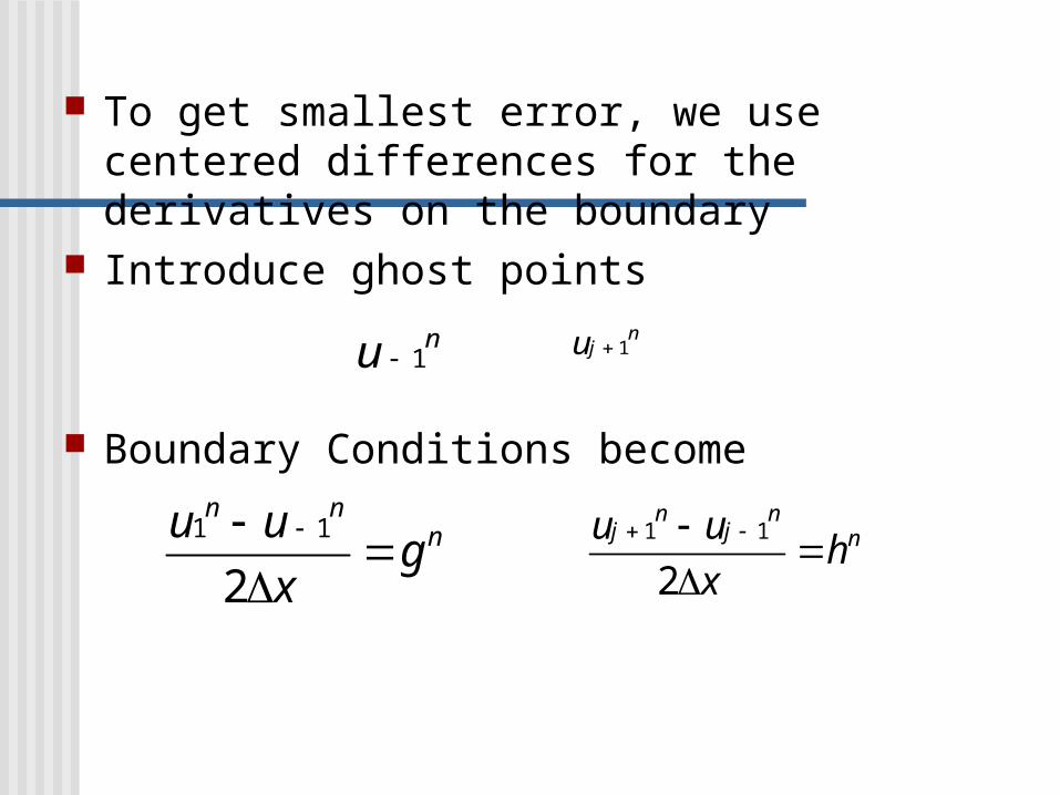
To get smallest error, we use centered differences for the derivatives on the boundary

Introduce ghost points

Boundary Conditions become 1nu 1

nju

1 1

2

n nnu u

gx

1 1

2

n nj j nu u

hx

Crank-Nicolson Scheme

Can avoid any restrictions on stability conditions

Unconditionally stable no matter what the value of s is.

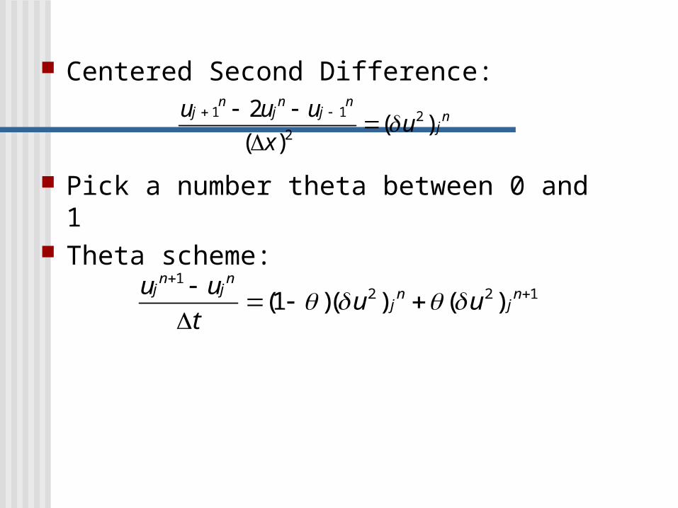
Centered Second Difference:

Pick a number theta between 0 and 1 Theta scheme:

1 1 22

2( )

( )

n n nj j j n

ju u u

ux

12 2 1(1 )( ) ( )

n nj j n n

j ju u

u ut

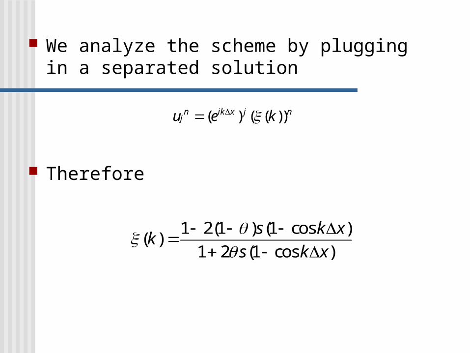
We analyze the scheme by plugging in a separated solution

Therefore

1 2(1 ) (1 cos )( )

1 2 (1 cos )

s k xk

s k x

( ) ( ( ))n ik x j nju e k

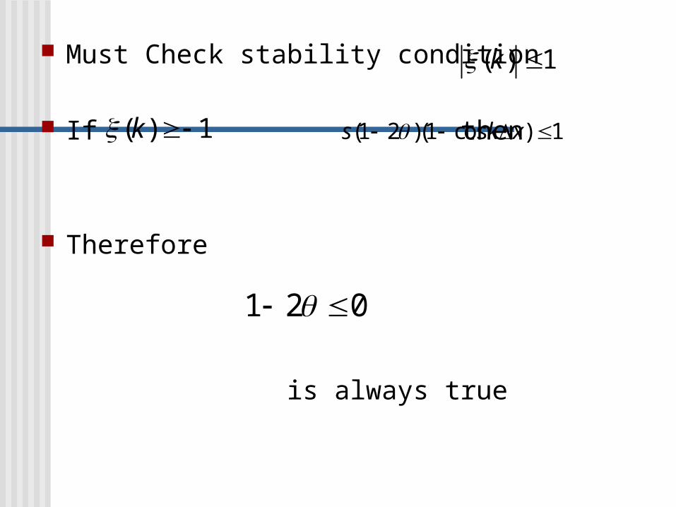
Must Check stability condition

If then

Therefore

is always true

( ) 1k

( ) 1k (1 2 )(1 cos ) 1s k x

1 2 0

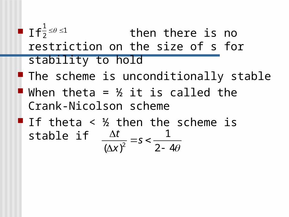
If then there is no restriction on the size of s for stability to hold

The scheme is unconditionally stable When theta = ½ it is called the Crank-Nicolson

scheme If theta < ½ then the scheme is stable if

11

2

2

1

( ) 2 4

ts

x

Stability Criterion

Approximations of the diffusion equation, ut=uxx

David Goldberg

Stability Criterion

The method of finite differences gives an answer, but it does not guarantee that this answer is meaningful.

Values must be chosen appropriately, to ensure that the results make sense and are applicable to real world scenarios.

This condition, that values must satisfy in order to be worthwhile, is called the “stability criterion.”

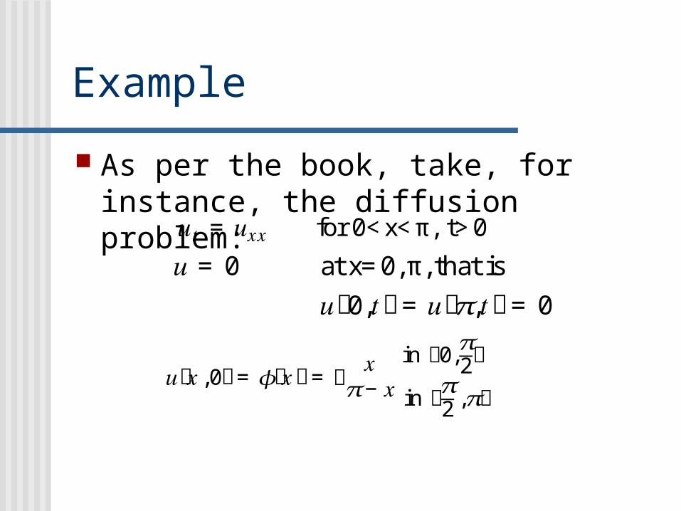
Example

As per the book, take, for instance, the diffusion problem:

𝑢ሺ𝑥,0ሻ= 𝜙ሺ𝑥ሻ= ቐ𝑥𝜋− 𝑥in ቀ0,𝜋2ቁ in ቀ𝜋2,𝜋ቁ

𝑢𝑡 = 𝑢𝑥𝑥 for 0<x<π, t>0 𝑢 = 0 at x=0, π, that is

𝑢ሺ0,𝑡ሻ= 𝑢ሺ𝜋,𝑡ሻ= 0

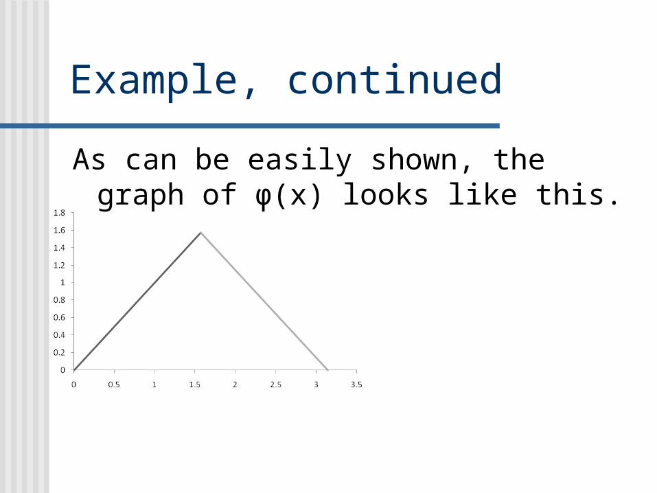
Example, continued

As can be easily shown, the graph of φ(x) looks like this.

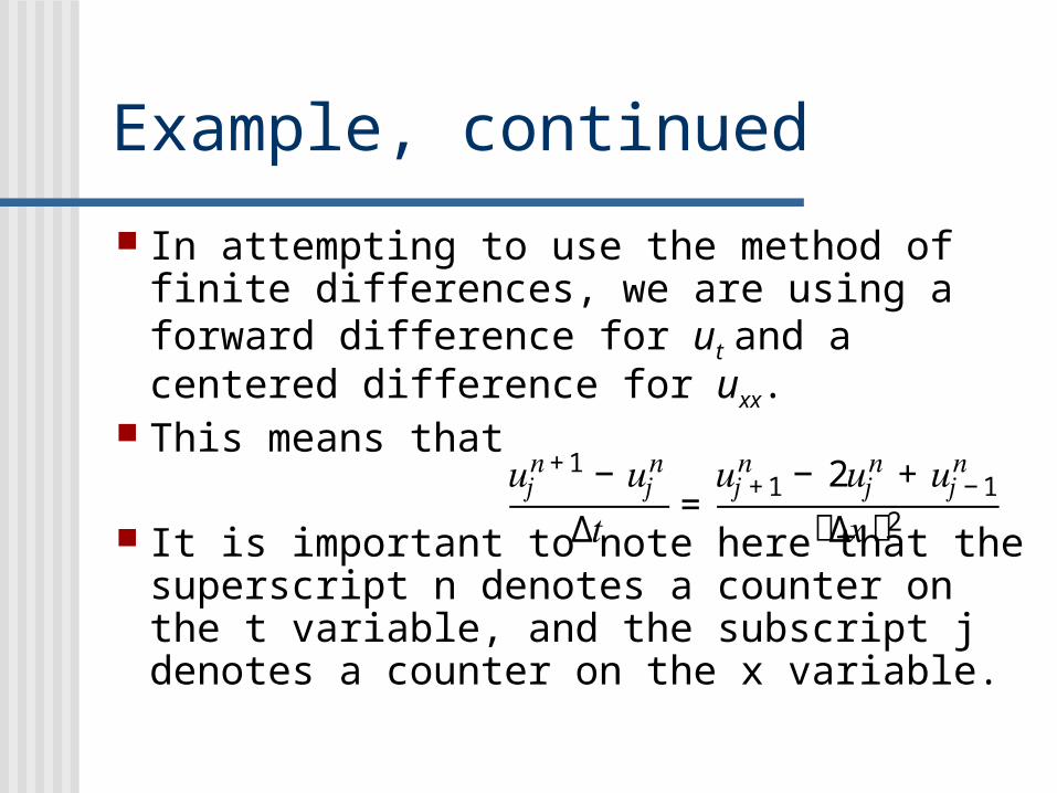
Example, continued

In attempting to use the method of finite differences, we are using a forward difference for ut and a centered difference for uxx.

This means that

It is important to note here that the superscript n denotes a counter on the t variable, and the subscript j denotes a counter on the x variable.

𝑢𝑗𝑛+1 − 𝑢𝑗𝑛Δ𝑡 = 𝑢𝑗+1𝑛 − 2𝑢𝑗𝑛 + 𝑢𝑗−1𝑛ሺΔ𝑥ሻ2

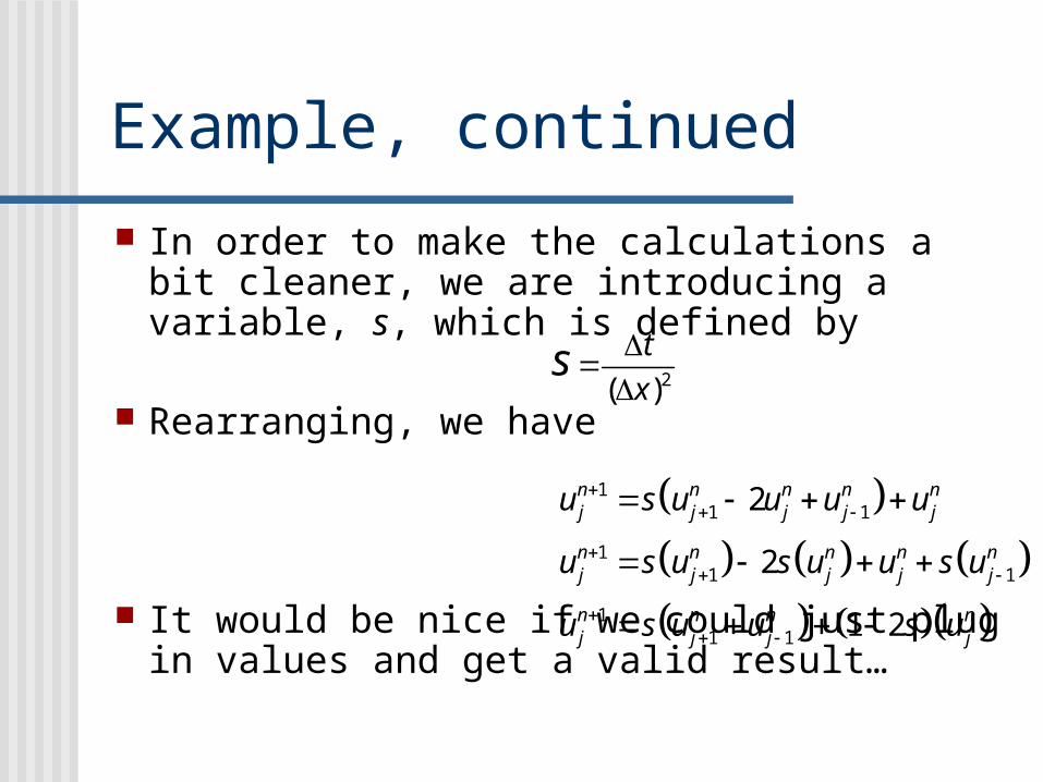
Example, continued

In order to make the calculations a bit cleaner, we are introducing a variable, s, which is defined by

Rearranging, we have

It would be nice if we could just plug in values and get a valid result…

2( )

t

xs

11 1

11 1

11 1

2

2

1 2

n n n n nj j j j j

n n n n nj j j j j

n n n nj j j j

u s u u u u

u s u s u u s u

u s u u s u

Example, continued

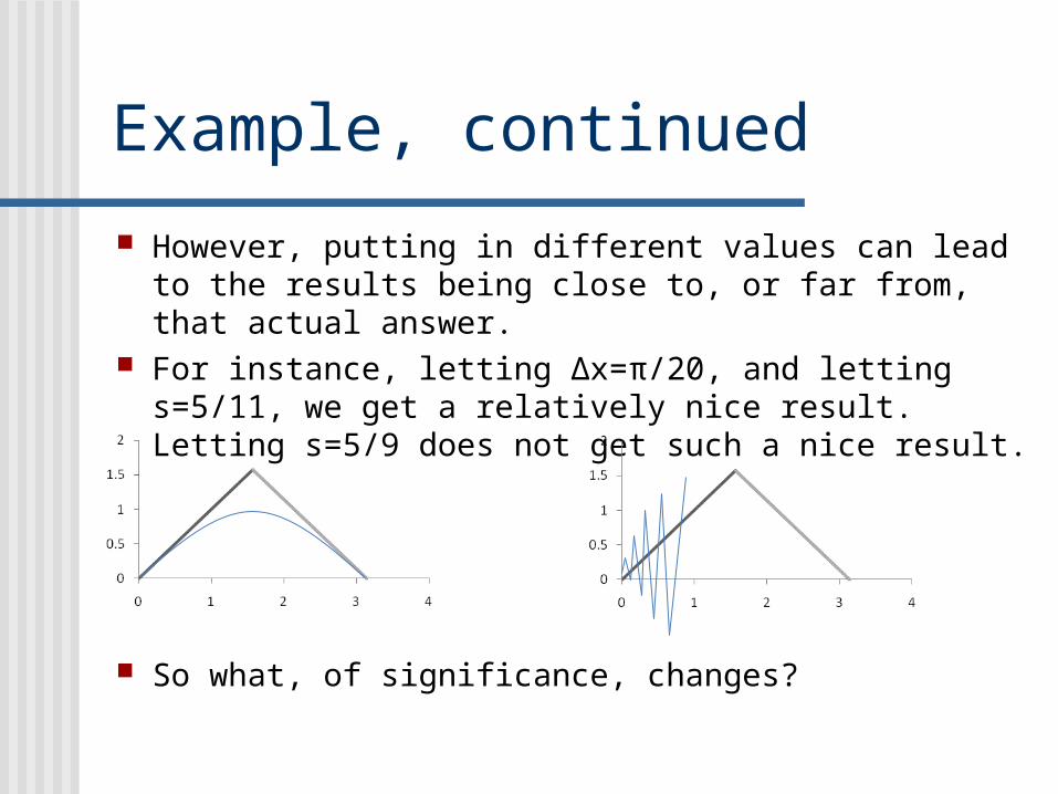
However, putting in different values can lead to the results being close to, or far from, that actual answer.

For instance, letting ∆x=π/20, and letting s=5/11, we get a relatively nice result. Letting s=5/9 does not get such a nice result.

So what, of significance, changes?

Example, Continued

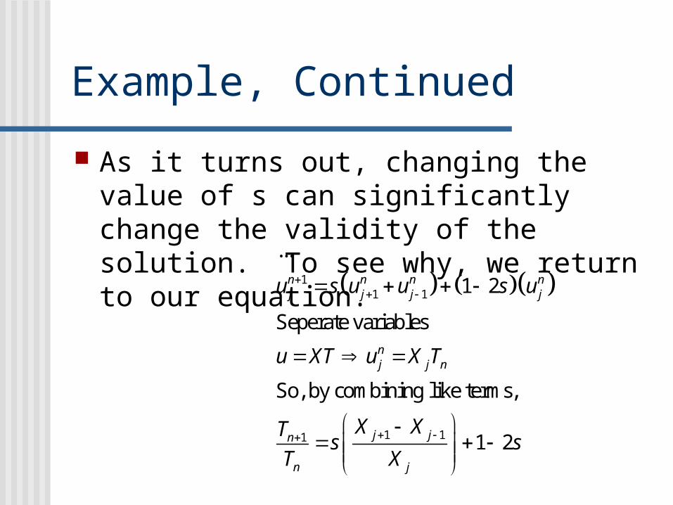
As it turns out, changing the value of s can significantly change the validity of the solution. To see why, we return to our equation.

11 1

1 11

...

1 2

Seperate variables

So, by combining like terms,

1 2

n n n nj j j j

nj j n

j jn

n j

u s u u s u

u XT u X T

X XTs s

T X

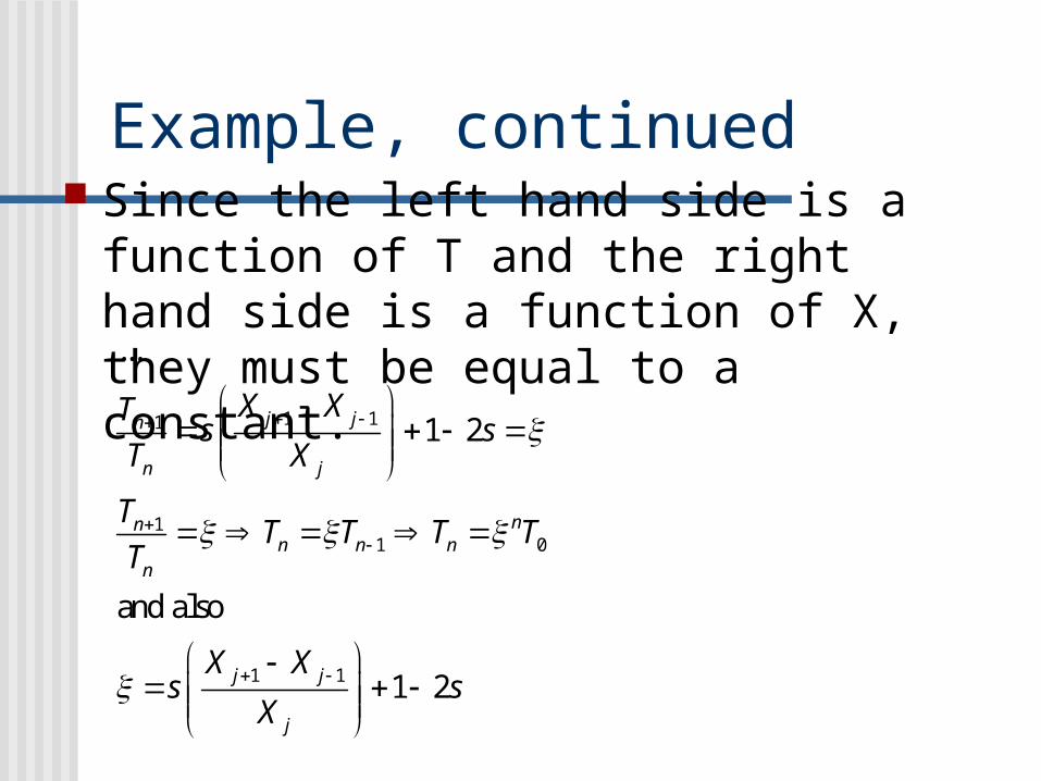
Example, continued Since the left hand side is a function of T

and the right hand side is a function of X, they must be equal to a constant.

1 11

11 0

1 1

...

1 2

and also

1 2

j jn

n j

nnn n n

n

j j

j

X XTs s

T X

TT T T T

T

X Xs s

X

Example, continued

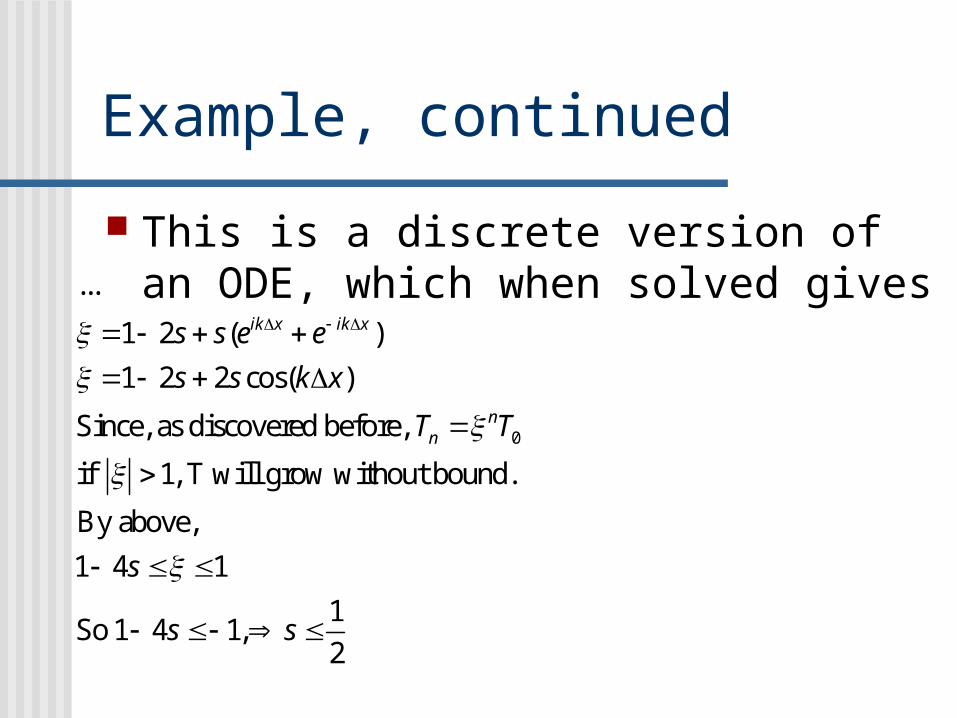
This is a discrete version of an ODE, which when solved gives

0

...

1 2 ( )

1 2 2 cos( )

Since, as discovered before,

if 1, T will grow without bound.

By above,

1 4 1

1So 1 4 1,

2

ik x ik x

nn

s s e e

s s k x

T T

s

s s

Example, finished

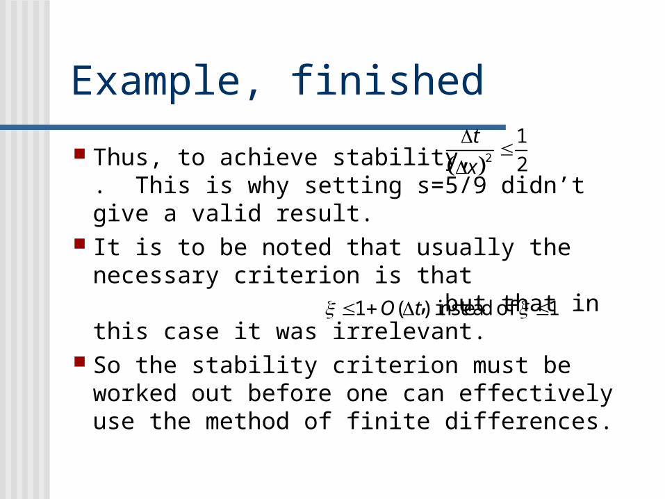
Thus, to achieve stability, . This is why setting s=5/9 didn’t give a valid result.

It is to be noted that usually the necessary criterion is that , but that in this case it was irrelevant.

So the stability criterion must be worked out before one can effectively use the method of finite differences.

1 ( ) instead of 1O t

2

1

2

t

x

Approximations of Diffusions

Example from 8.2

Daniel Rave

Summary

Breif Review of Methods

Wide Applicability

Importance of Stability