Embed Size (px)
Citation preview
Numerical modelling of the blowing phase in the productionof glass containers
W. Dijkstra∗a, R.M.M. Mattheij∗
∗Department of Mathematics and Computing Science, Eindhoven University of Technology,
P.O. Box 513, 5600 MB Eindhoven, The Netherlands
Abstract
The industrial manufacturing of glass containers consistsof several phases, one of which is the blowingphase. This paper describes the development of a numerical simulation tool for this phase. The hot liquidglass is modelled as a viscous fluid and its flow is governed by the Stokes equations. We use the boundaryelement method to solve the Stokes equations and obtain the velocity profile at the glass surface. Themovement of the surface obeys an ordinary differential equation. We describe three methods to performa time integration step and update the shape of the glass surface. All calculations are performed in threedimensions. This allows us to simulate the blowing of glass containers that are not rotationally symmetric.The contact between glass and mould is modelled using a partial-slip condition. A number of simulationson model glass containers illustrates the results.
Keywords: Boundary element method, blowing phase, glass, Stokes equations
1 Introduction
The industrial production of glass products like bottles and jars consists of several phases. First glass ismelted in a furnace where the glass reaches temperatures between1200 and1600 oC. The molten glass isthen cut intogobs, which are transported to a forming machine.
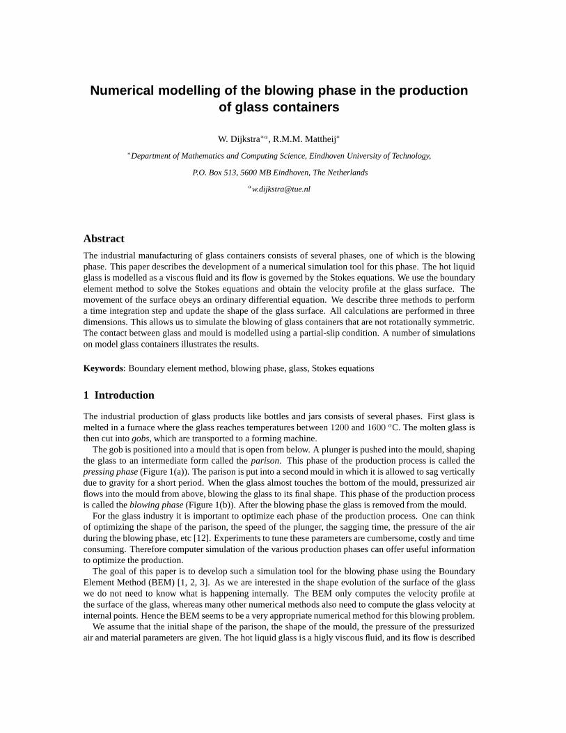
The gob is positioned into a mould that is open from below. A plunger is pushed into the mould, shapingthe glass to an intermediate form called theparison. This phase of the production process is called thepressing phase(Figure 1(a)). The parison is put into a second mould in whichit is allowed to sag verticallydue to gravity for a short period. When the glass almost touches the bottom of the mould, pressurized airflows into the mould from above, blowing the glass to its final shape. This phase of the production processis called theblowing phase(Figure 1(b)). After the blowing phase the glass is removed from the mould.
For the glass industry it is important to optimize each phaseof the production process. One can thinkof optimizing the shape of the parison, the speed of the plunger, the sagging time, the pressure of the airduring the blowing phase, etc [12]. Experiments to tune these parameters are cumbersome, costly and timeconsuming. Therefore computer simulation of the various production phases can offer useful informationto optimize the production.
The goal of this paper is to develop such a simulation tool forthe blowing phase using the BoundaryElement Method (BEM) [1, 2, 3]. As we are interested in the shape evolution of the surface of the glasswe do not need to know what is happening internally. The BEM only computes the velocity profile atthe surface of the glass, whereas many other numerical methods also need to compute the glass velocity atinternal points. Hence the BEM seems to be a very appropriatenumerical method for this blowing problem.
We assume that the initial shape of the parison, the shape of the mould, the pressure of the pressurizedair and material parameters are given. The hot liquid glass is a higly viscous fluid, and its flow is described
(a) Pressing phase (b) Blowing phase
Figure 1:The production of glass containers consists of a pressing phase and a blowing phase.
by the Stokes equations. The BEM computes the flow at the surface of the glass solving these Stokesequations. Then we perform a time integration step to obtainthe shape of the glass at the next time level.For this new shape we again compute the flow at the surface and perform another time integration step.This iterative procedure enables us to study the shape evolution of the glass during the blowing phase.The computations are performed in three dimensions. This allows us to study bottles and jars that are notrotationally symmetric, for instance due to small imperfections in the initial parison.
Numerical modelling of the production process of glass bottles and jars has been the topic of severalpapers. Mostly finite elements are used to solve the Stokes equations [5, 6], sometimes using a level setmethod to track the position of the glass surface [8]. In manycases rotationally symmetric parisons aremodelled and computations are thus limited to two dimensions. To the authors knowledge our work is thefirst to address the blowing problem in three dimensions using the BEM.
During the blowing phase the temperature of the glass changes due to heat exchange with the mould.The viscosity of the glass depends on the temperature in an essentially non-linear way. Hence the heatproblem and the flow problem are coupled. In the papers mentioned above this phenomenon is studiedintensively. In this paper we assume a uniform temperature field that may vary in time.
Special attention has to be given to the contact problem of the glass and the mould. Most papers assumea no-slip condition at the mould. In practice this is not the case. Sometimes the mould is even covered witha lubricating substance to improve the slip of the glass. Therefore we choose to work with a partial-slipboundary condition instead of a no-slip boundary condition.
The procedure described above results in a simulation tool to study the blowing phase for glass products.We have tested the simulation tool on several bottles and jars. The results of the tests are promising andmay contribute to a better understanding of the production of bottles and jars.
This paper is set up as follows. Section 2 introduces the mathematical model of the glass flow duringthe blowing phase. The boundary value problem that we derivein this section is solved with the boundaryelement method in Section 3. In Section 5 we present a number of tests to show the performance of thesimulation tool. We conclude with a short discussion in Section 6
2 Mathematical model
In this section we derive the mathematical model that describes the flow of a three-dimensional volume ofNewtonian fluid with high viscosity.
We consider a volume of fluid in three dimensions denoted byΩ. The fluid is bounded by a closedsurfaceS. The velocity and pressure of the fluid are denoted byv andp respectively. Furthermore the fluid
is characterized by the dynamic viscosityη, the surface tensionγ and a typical length scaleL.The motion of the fluid is governed by two equations. The continuity equation expresses conservation
of mass, and reads
∇.v = 0, (1)
where we assumed that the density of the fluid is constant and uniform, i.e. the fluid is incompressible. Asthe fluid is highly viscous, the conservation of momentum is described by the Stokes equations,
∇.σ + ρg = 0, (2)
whereg is a body force (here we consider only gravitational forceg = −gez) andσ is the stress tensor.For the Newtonian fluid the following constitutive equationfor the stress tensor holds,
σij := −pδij + η
(
∂vi
∂xj
+∂vj
∂xi
)
, (3)
with δij the Kronecker delta. Substitution of the constitutive equation forσ into the Stokes equations yields
η∇2v −∇p+ ρg = 0. (4)
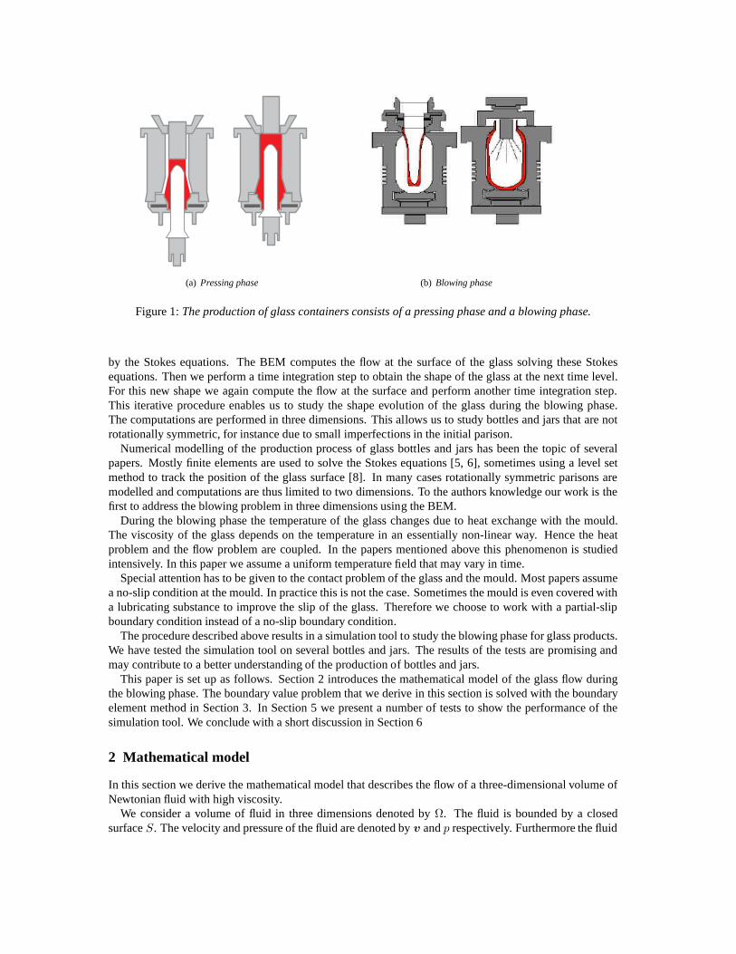
S 0
S 1
S 2
W
S 3
Figure 2:The surface of the glass is divided into four parts (cross-sectional view).
We distinguish four types of boundary conditions, see Figure 2. At the surfacesS0 andS1 the normalstress is related to the prescribed pressuresp0 andp1 onto the surface and the surface tensionγ,
σn = −p0n− γκn, atS0,
σn = −p1n− γκn, atS1. (5)
The vectorn is the outward unit normal at the surface andκ is the mean curvature at a certain point ofthe surface. The first term in the boundary condition accounts for the external pressure acting onto thesurface. The second term accounts for the surface tension due to the curvature of the surface. In the fluidall molecules attract one another. A molecule that is in the interior of the fluid domain is attracted by allits neighbours, so the average force it experiences is equalto zero. A molecule at the surface of the fluidexperiences a force inwards the fluid. For highly curved surfaces this force will be larger than for flatsurfaces. The curvature of the surface is measured by themean curvatureκ with dimensionL−1. For moredetails about the incorporation of curvature in the boundary conditions we refer to [16].
At the surfaceS2 the glass is not allowed to move and hence we set the velocity equal to zero,
v = 0, atS2. (6)
At the surfaceS3 the fluid is in contact with a solid wall, but is allowed to slipalong the wall. This meansthat the velocity component in the normal direction is equalto zero, i.e. the fluid cannot penetrate throughthe wall,
v.n = 0, atS3. (7)
The velocity component in the tangential directions does not need to be zero. The most common conditionis that the tangential component of the velocity is related to the normal stress by [9],
(σn+ βmv).t = 0, atS3. (8)
Heret is a vector in the tangential direction at the wall andβm is a friction parameter. Ifβm → 0 there isno friction between fluid and wall. Ifβm → ∞ the friction between fluid and wall is too large to allow slipalong the wall. It can be seen that in that case (7) together with (8) yield the no-slip condition (6).
Let vc be a characteristic velocity for the flow of the fluid. We definea characteristic pressurepc bypc = ηvc/L. Using these characteristic parameters and usingL as a characteristic length, we rewrite theNavier-Stokes equations in dimensionless form,
∇′2v′ −∇′p′ + αg′ = 0. (9)
Herev′, p′ andg′ are the dimensionless velocity, pressure and body force, and the differential operator∇′
denotes differentiation with respect to the dimensionlessspatial coordinates. The dimensionless parameterα is the ratio of the Reynolds number and the Froude number, defined as
Re :=ρLvc
η, Fr :=
v2c
gL, (10)
whereg is the acceleration of gravity. The dimensionless form of the momentum balance (9) together withthe dimensionless form of the mass balance (1),
∇′.v′ = 0, (11)
give a system of four equations that describe the flow of the fluid.It can be verified that the dimensionless stress tensorσ′ is defined as
σ′ := −p0
p1 − p0
I +1
p1 − p0
σ. (12)
We also introduce a dimensionless curvatureκ′ by κ′ = Lκ. Substitution ofσ′ andκ′ into the boundaryconditions atS0 andS1 yields
σ′n = −βκ′n, atS0,
σ′n = −(1 + βκ′)n, atS1, (13)
where the dimensionless parameterβ is defined as
β :=γ
(p1 − p0)L. (14)
The boundary condition atS2 becomes
v′ = 0, atS2. (15)
It can be verified that substitution ofσ′ andv′ into the second part of the boundary condition atS3 yields
−p0n.t+ (p1 − p0)(σ′n+
Lβm
ηv′).t = 0. (16)
The first term cancels out sincen.t = 0. We divide byp1 − p0 and and get the following boundaryconditions atS3,
(σ′n+ β′
mv′).t = 0,
v′.n = 0, atS3, (17)
where the dimensionless friction parameterβ′
m is defined as
β′
m :=Lβm
η. (18)
In the sequel we drop the′ to simplify the notation.We introduce a modified pressurep by [13, p. 164]
p := p+ αz, (19)
wherez is the vertical coordinate. Since∇p = ∇p+ αez = ∇p+ αg, the momentum balance simplifiesto
∇2v −∇p = 0, in Ω. (20)
We may define a modified stress tensorσ by
σ := σ(p,v) = −αzI + σ(p,v). (21)
Substitution of this new stress tensor into the boundary conditions atS0 andS1 yields
σn = −(αz + βκ)n, atS0,
σn = −(1 + αz + βκ)n, atS1. (22)
It can be verified that substitution ofσ into the second part of the boundary condition atS3 yields
αzn.t+ (σn+ βmv).t = 0. (23)
The first term cancels out sincen.t = 0 and we obtain the following conditions atS3,
(σn+ βmv).t = 0,
v.n = 0, atS3, (24)
To summarize, the equations and boundary conditions in dimensionless form are given by
∇2v −∇p = 0, in Ω,
∇.v = 0, in Ω,
σn = −(αz + βκ)n, atS0,
σn = −(1 + αz + βκ)n, atS1,
v = 0, atS2,
(σn+ βmv).t = 0, atS3,
v.n = 0, atS3. (25)
In the sequel we will omit theto simplify the notation.
3 Boundary element method
We use the boundary element method to solve the Stokes problem outlined in the previous section. Firstwe show how the boundary value problem transforms into a set of boundary integral equations. Afterdiscretisation of the surface we obtain a linear system of algebraic equations. Solving this system yieldsthe velocity of the glass surface.
The key ingredient to transform the mathematical model fromhe previous section into a set of boundaryintegral equations is Green’s identity for the Stokes problem. For an extensive derivation we refer thereader to [11].
We introduce a new variableb,
b := σ(p,v)n, (26)
which represents the normal stress at the boundary. Under the assumption that the surface ofΩ is smooth,it can be deduced that
1
2δijvj(x) +
∫
S
qij(x,y)vj(y)dSy =
∫
S
uij(x,y)bj(y)dSy, i = 1, 2, 3, x ∈ S. (27)
Here the functionsqij anduij are defined as
qij(x,y) :=3
4π
(xi − yi)(xj − yj)(xk − yk)nk
‖x− y‖5
uij(x,y) :=1
8π
[
δij1
‖x− y‖+
(xi − yi)(xj − yj)
‖x− y‖3
]
. (28)
We introduce the integral operatorsG andH,
(Gφ)i :=
∫
S
uij(x,y)φj(y)dSy ,
(Hψ)i :=
∫
S
qij(x,y)ψj(y)dSy . (29)
These operators are the single and double layer operator forthe Stokes flow respectively. With theseoperators the boundary integral equation (27) is simply as,
(1
2I + H
)
v = Gb. (30)
This boundary integral equation expresses the relation between the flowv of the surface of the fluid andthe normal stressesb at the surface.
The surfaceS is approximated byK linear triangular elements. Each element typically consists of threenodesx1, x2, x3 that are located at the corners of the triangle. The total number of nodes is denoted byN . We introduce three linear shape functions,
φ1(ξ1, ξ2) = 1 − ξ1 − ξ2,
φ2(ξ1, ξ2) = ξ1,
φ3(ξ1, ξ2) = ξ2, (31)
where0 ≤ ξ1, ξ2 ≤ 1 andξ1 + ξ2 ≤ 1. Consider thek-th elementSk with nodesx1, x2 andx3. TheelementSk is parameterized by
y = y(ξ1, ξ2) = φ1x1 + φ2x
2 + φ3x3. (32)
The vectorsv andb are linearly approximated with the same shape functions,
v(y) = φ1v1 + φ2v
2 + φ3v3,
b(y) = φ1b1 + φ2b
2 + φ3b3. (33)
Herevs = v(xs) is the velocity at the nodexs andbs = b(xs) is the normal stress at the nodexs. Weapproximate the surface integral overS in (27) by a sum of integrals over the elementsSk, and substitutethe approximations forv andb,
1
2vi(x) +
K∑
k=1
∫
Sk
qij(x,y)(
φ1v1j + φ2v
2j + φ3v
3j
)
dSy
=
K∑
k=1
∫
Sk
uij(x,y)(
φ1b1j + φ2b
2j + φ3b
3j
)
dSy, x ∈ S, i = 1, 2, 3. (34)
We substitutex = xp, p = 1, . . . , N , in (34), obtaining3N equations. Next we construct two coefficientvectors,
v =[
v11 , v
12 , v
13 , . . . , v
N1 , v
N2 , v
N3
]T,
b =[
b11, b12, b
13, . . . , b
N1 , b
N2 , b
N3
]T. (35)
This allows us to write (34) in a matrix-vector form,
Hv = Gb. (36)
To compute the matricesH andG, we have to evaluate integrals of the form∫
Sk
qij(xp,y)φrdSy,
∫
Sk
uij(xp,y)φrdSy. (37)
The integrals can be evaluated by using a Gauss quadrature scheme, but special care has to be taken whenthe nodexp is in the surface elementSk. In that case one need to use a slightly more elaborate methodtoevaluate the integrals, e.g. a logarithmic Gauss quadrature scheme.
In the case whereS3 = ∅ we either know the velocity coefficients at a node or the normal stress co-efficients. Hence in (36) some of the unknowns are in the vector b at the right-hand side and some ofthe knowns are in the vectorv at the left-hand side. By interchanging columns properly wearrive at thestandard form linear system with unknownx,
Ax = f . (38)
WhenS3 6= ∅ there are nodes at which both the velocity and normal stress coefficients are unknown,though related via the slip conditions (24). Lettr, r = 1, 2, be the two tangential vectors at the wall at sucha nodex ∈ S3. Sincev.n = 0 atx, we may write
v(x) = a1t1(x) + a2t
2(x), a1, a2 ∈ R. (39)
Substitution into(b+βmv).tr = 0 yieldsar = −(b.tr)/βm. In the boundary integral equation we replace
v(x) by the above expression. Thus we have eliminatedv(x) and the only uknown atx is b(x). Thesolution of the BEM yields the normal stressb(x) and as a post-processing step we compute the velocityv(x) from (39). In this way we arrive at the same standard form linear systemAx = f .
The matrixA is a dense matrix and the linear system can be solved by using an LU-decompositiontechnique. Due to the dense nature of the matrix, this may become costly, especially when the size of thematrix is large.
4 Algorithm
In this section we describe an algorithm to simulate the blowing phase. Several steps can be distinguishedin this algorithm.
Initial surface Sfor step = 1, 2, ...
Use BEM to obtain vPerform velocity smoothingPerform time integration to update SPerform Laplacian smoothingRegridding
end
Time integration
The movement of the surface of the fluid domain is described bythe velocity fieldv(x, t) that is theoutcome of the Stokes problem. In fact we calculate the velocity at a set ofN nodes at the surface. Tostudy the evolution of the surface we need to solve an ordinary differential equation,
∂x
∂t= v(x, t), x ∈ S. (40)
Assume that at timet = tn we know the locations of the nodesxn and the velocity at these nodesv(xn, tn) =: vn. We do not have any information of the nodes or velocity in thefuture. Thereforewe cannot make use of implicite time integration schemes to solve (40).
An option is to use anEuler forwardscheme, in which we approximate the locations of the nodes atthenext time leveltn+1 by
xn+1 = xn + ∆tv(xn, tn). (41)
However this scheme is only first order accurate. Another option is to use a modified version ofHeun’smethod, which is also called theimproved Euler method. This method is known to be second order accurate[4]. However for this method we need the velocityv at the next time leveltn+1 in the new locationxn+1
of the node. As we remarked before we do not have information of future time levels. To get around thisproblem we first predict the location of the node at the next time level using a Euler forward step (41). Forthis predicted nodexn+1 we again solve the Stokes problem and we obtain the velocity in this node at timetn+1. Then we update our prediction ofxn+1 with Heun’s method. In this way we corrected the predictionof xn+1 as performed with the Euler forward step. The disadvantage of the Heun’s method is that we haveto solve two Stokes problems at each time step.
A third option to perform time integration is the so calledflow methoddeveloped in [14]. Time in-tegration is explicit in this method and only one Stokes problem needs to be solved at each time step,while accuracy is second order. To reach this quadratic accuracy an inverse interpolation problem is solvedat each time step. The method exploits the fact that the time-dependence of the velocity is very small,∂v/∂t ≈ 0, and hence we have to solve an ODE of the form∂x/∂t = v(x). Another advantage of theflow method is its volume-conserving nature. Also on the longterm this method performs better than othersecond order methods. However, the time interval that is spanned in our simulations is very restricted, sowe cannot exploit the long term performance of the flow method.
Note that the BEM with linear elements as described in the previous section is second order accurate.This means that we cannot improve the overall accuracy by choosing an accurate time integration methodonly. We also need to use higher order elements in the BEM to achieve high accuracy. To illustrate this,we may monitor the total volume of the fluid domain. As we are dealing with an incompressible fluid, thevolume should remain constant during the blowing phase. Hence computation of the fluid volume at eachtime step provides us insight in the accuracy of the simulation tool.
At each node at the surface the BEM computes the velocity withan error of orderh2, whereh is atypical size of the boundary elements. Summation over all elements yields an error of orderh in the totalvolume. From that point of view it does not make any difference if we use a first or second order ac-curate time integration scheme. The error in the fluid volumeis always dominated by the error made bythe BEM. Hence in our simulation we always choose the Euler forward method to perform time integration.
Laplacian smoothing
A well-known technique to smooth a triangulated surface isLaplacian smoothing[7, 10, 17]. For eachnodex at the surfaceS we compute the geometric averagexav of the neighbouring nodes. A neighbouringnode is a node that shares an edge of a triangle withx. If the nodex is too far away fromxav, it is relocatedat the geometric average. Or more general, the nodex is replaced by a weighted average ofx andxav,
x→ (1 − w)x+ wxav, (42)
wherew is a suitably chosen weight. We can do this for every node, in which case we applyglobalsmoothing. Or we may replacex only if the distance toxav exceeds a certain tolerance. In that case we
apply local smoothing. In other words, we smooth the surface only at nodes where it is most needed. Theprocess can be repeated several times. In each iteration thesurface gets smoother.
A side-effect of the smoothing is that the volume that the surface encloses decreases. This is a typicaldisadvantage of standard Laplacian smoothing. There are several modifications to the standard technique toavoid volume loss. The simplest one is to restrict the movement of the nodex to a direction perpendicularto the normal at the surface atx. Unfortunately this reduces the performance of the smoothing. Anotherpossibility is to take pairs of nodes that are connected by anedge. The two nodes are relocated to newpositions simultaneously. In this way we have more freedom to move the nodes to the desired locations,while conserving the volume. In our simulation tool we use the latter modification to Laplacian smoothing.For more details we refer to [10].
Regridding
As the deformation of the glass is large the triangular elements of the discretised surfaceS may becomevery large. Therefore it is necessary to remesh the surface regularly. At every time step of the simulationwe monitor the length of the egdes of the boundary elements. If such an edge has a length larger than acertain tolerance level, this edge is subdivided. As a consequence the two elements that share this edge aresubdivided into four new elements.
5 Results
In this section we perform several simulations with model glass parisons that are blown to bottles or jars.In all simulations we assume that the top of the parison is fixed, i.e. the velocity of the glass is equal tozero. This part of the glass corresponds to the surface partS2 (see Figure 2).
The material properties of glass can be found in [15]. With these properties the dimensionless parametersthat appear in the model get the following values,
α = 0.0082, β = 0.001. (43)
Ideally, the value of the dimensionless friction coefficient βm has to be determined experimentally. How-ever, to the authors’ knowledge no such experiments have been reported in literature. For our simulationswe takeβm = 1, i.e. a partial-slip condition for the glass when it comes into contact with the wall.
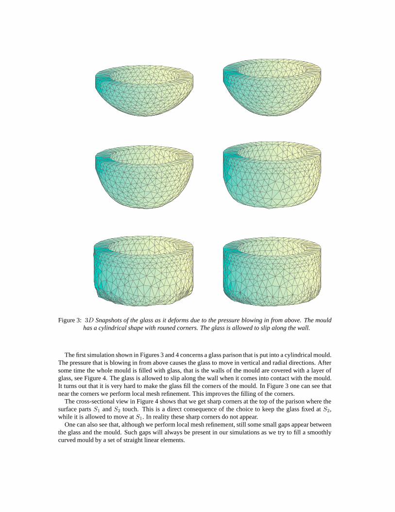
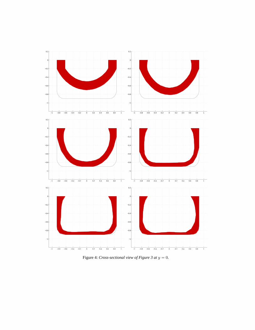
Figure 3: 3D Snapshots of the glass as it deforms due to the pressure blowing in from above. The mouldhas a cylindrical shape with rouned corners. The glass is allowed to slip along the wall.
The first simulation shown in Figures 3 and 4 concerns a glass parison that is put into a cylindrical mould.The pressure that is blowing in from above causes the glass tomove in vertical and radial directions. Aftersome time the whole mould is filled with glass, that is the walls of the mould are covered with a layer ofglass, see Figure 4. The glass is allowed to slip along the wall when it comes into contact with the mould.It turns out that it is very hard to make the glass fill the corners of the mould. In Figure 3 one can see thatnear the corners we perform local mesh refinement. This improves the filling of the corners.
The cross-sectional view in Figure 4 shows that we get sharp corners at the top of the parison where thesurface partsS1 andS2 touch. This is a direct consequence of the choice to keep the glass fixed atS2,while it is allowed to move atS1. In reality these sharp corners do not appear.
One can also see that, although we perform local mesh refinement, still some small gaps appear betweenthe glass and the mould. Such gaps will always be present in our simulations as we try to fill a smoothlycurved mould by a set of straight linear elements.
−1 −0.8 −0.6 −0.4 −0.2 0 0.2 0.4 0.6 0.8 1
−1
−0.8
−0.6
−0.4
−0.2
0
0.2
−1 −0.8 −0.6 −0.4 −0.2 0 0.2 0.4 0.6 0.8 1
−1
−0.8
−0.6
−0.4
−0.2
0
0.2
−1 −0.8 −0.6 −0.4 −0.2 0 0.2 0.4 0.6 0.8 1
−1
−0.8
−0.6
−0.4
−0.2
0
0.2
−1 −0.8 −0.6 −0.4 −0.2 0 0.2 0.4 0.6 0.8 1
−1
−0.8
−0.6
−0.4
−0.2
0
0.2
−1 −0.8 −0.6 −0.4 −0.2 0 0.2 0.4 0.6 0.8 1
−1
−0.8
−0.6
−0.4
−0.2
0
0.2
−1 −0.8 −0.6 −0.4 −0.2 0 0.2 0.4 0.6 0.8 1
−1
−0.8
−0.6
−0.4
−0.2
0
0.2
Figure 4:Cross-sectional view of Figure 3 aty = 0.
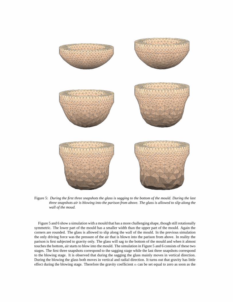
Figure 5: During the first three snapshots the glass is sagging to the bottom of the mould. During the lastthree snapshots air is blowing into the parison from above. The glass is allowed to slip along thewall of the moud.
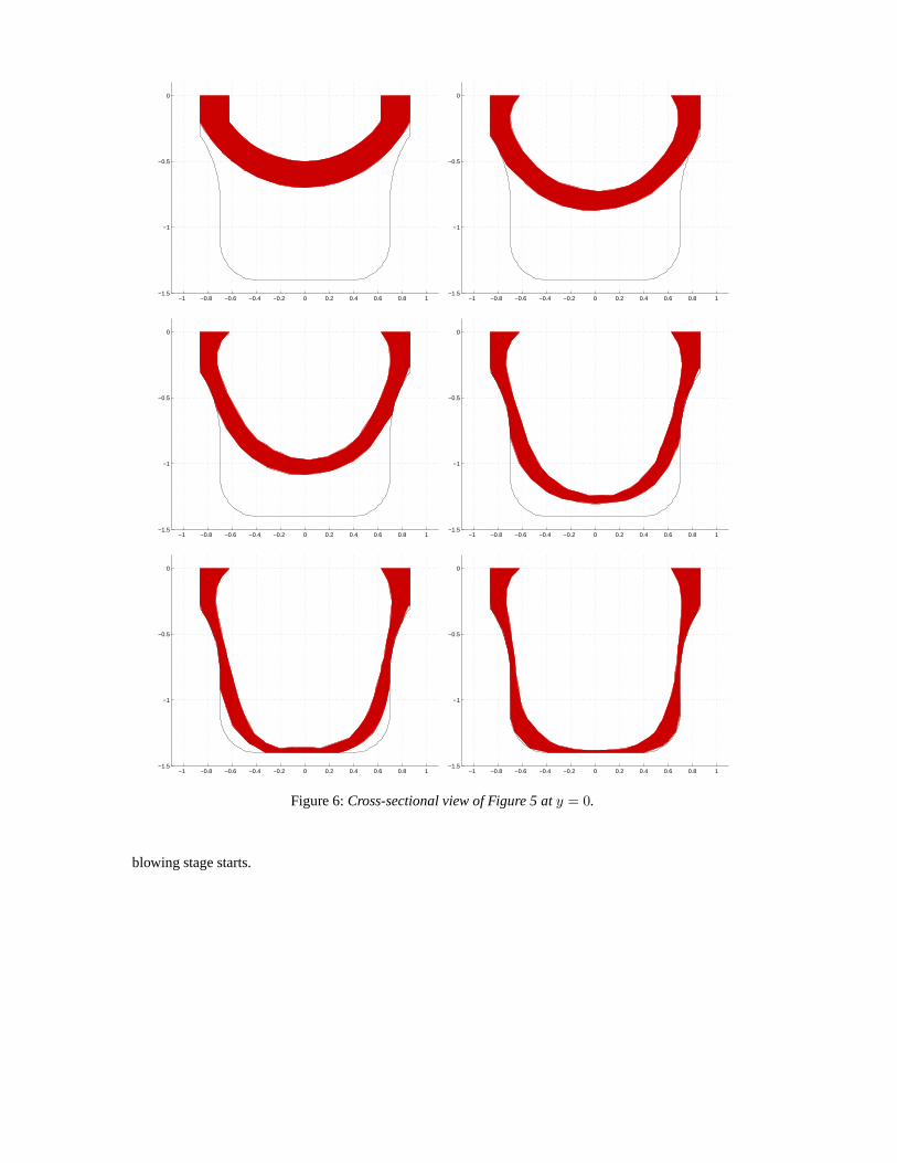
Figure 5 and 6 show a simulation with a mould that has a more challenging shape, though still rotationallysymmetric. The lower part of the mould has a smaller width than the upper part of the mould. Again thecorners are rounded. The glass is allowed to slip along the wall of the mould. In the previous simulationthe only driving force was the pressure of the air that is blown into the parison from above. In reality theparison is first subjected to gravity only. The glass will sagto the bottom of the mould and when it almosttouches the bottom, air starts to blow into the mould. The simulation in Figure 5 and 6 consists of these twostages. The first three snapshots correspond to the sagging stage while the last three snapshots correspondto the blowing stage. It is observed that during the sagging the glass mainly moves in vertical direction.During the blowing the glass both moves in vertical and radial direction. It turns out that gravity has littleeffect during the blowing stage. Therefore the gravity coefficientα can be set equal to zero as soon as the
−1 −0.8 −0.6 −0.4 −0.2 0 0.2 0.4 0.6 0.8 1−1.5
−1
−0.5
0
−1 −0.8 −0.6 −0.4 −0.2 0 0.2 0.4 0.6 0.8 1−1.5
−1
−0.5
0
−1 −0.8 −0.6 −0.4 −0.2 0 0.2 0.4 0.6 0.8 1−1.5
−1
−0.5
0
−1 −0.8 −0.6 −0.4 −0.2 0 0.2 0.4 0.6 0.8 1−1.5
−1
−0.5
0
−1 −0.8 −0.6 −0.4 −0.2 0 0.2 0.4 0.6 0.8 1−1.5
−1
−0.5
0
−1 −0.8 −0.6 −0.4 −0.2 0 0.2 0.4 0.6 0.8 1−1.5
−1
−0.5
0
Figure 6:Cross-sectional view of Figure 5 aty = 0.
blowing stage starts.
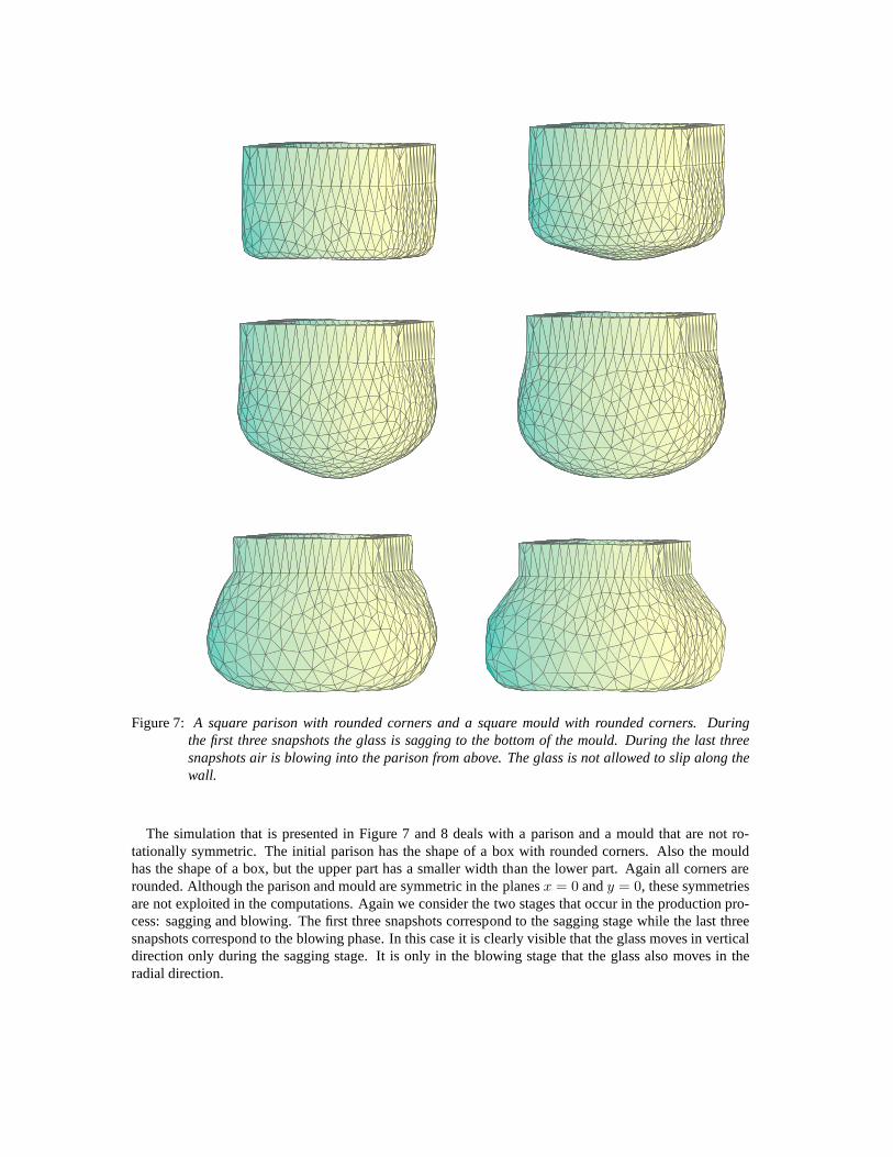
Figure 7: A square parison with rounded corners and a square mould withrounded corners. Duringthe first three snapshots the glass is sagging to the bottom ofthe mould. During the last threesnapshots air is blowing into the parison from above. The glass is not allowed to slip along thewall.
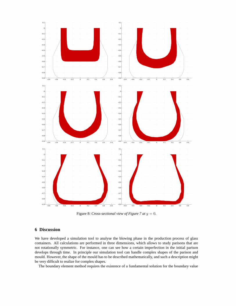
The simulation that is presented in Figure 7 and 8 deals with aparison and a mould that are not ro-tationally symmetric. The initial parison has the shape of abox with rounded corners. Also the mouldhas the shape of a box, but the upper part has a smaller width than the lower part. Again all corners arerounded. Although the parison and mould are symmetric in theplanesx = 0 andy = 0, these symmetriesare not exploited in the computations. Again we consider thetwo stages that occur in the production pro-cess: sagging and blowing. The first three snapshots correspond to the sagging stage while the last threesnapshots correspond to the blowing phase. In this case it isclearly visible that the glass moves in verticaldirection only during the sagging stage. It is only in the blowing stage that the glass also moves in theradial direction.
−0.8 −0.6 −0.4 −0.2 0 0.2 0.4 0.6 0.8−0.9
−0.8
−0.7
−0.6
−0.5
−0.4
−0.3
−0.2
−0.1
0
0.1
−0.8 −0.6 −0.4 −0.2 0 0.2 0.4 0.6 0.8−0.9
−0.8
−0.7
−0.6
−0.5
−0.4
−0.3
−0.2
−0.1
0
0.1
−0.8 −0.6 −0.4 −0.2 0 0.2 0.4 0.6 0.8−0.9
−0.8
−0.7
−0.6
−0.5
−0.4
−0.3
−0.2
−0.1
0
0.1
−0.8 −0.6 −0.4 −0.2 0 0.2 0.4 0.6 0.8−0.9
−0.8
−0.7
−0.6
−0.5
−0.4
−0.3
−0.2
−0.1
0
0.1
−0.8 −0.6 −0.4 −0.2 0 0.2 0.4 0.6 0.8−0.9
−0.8
−0.7
−0.6
−0.5
−0.4
−0.3
−0.2
−0.1
0
0.1
−0.8 −0.6 −0.4 −0.2 0 0.2 0.4 0.6 0.8−0.9
−0.8
−0.7
−0.6
−0.5
−0.4
−0.3
−0.2
−0.1
0
0.1
Figure 8:Cross-sectional view of Figure 7 aty = 0.
6 Discussion
We have developed a simulation tool to analyse the blowing phase in the production process of glasscontainers. All calculations are performed in three dimensions, which allows to study parisons that arenot rotationally symmetric. For instance, one can see how a certain imperfection in the initial parisondevelops through time. In principle our simulation tool canhandle complex shapes of the parison andmould. However, the shape of the mould has to be described mathematically, and such a description mightbe very difficult to realize for complex shapes.
The boundary element method requires the existence of a fundamental solution for the boundary value
problem. For the Stokes equations such a fundamental solution can be found, provided that the coefficientsin the Stokes equations are constant. However, for hot liquid glass the material parameters are known to bet emperature-dependent, in particular the viscosity. As the temperature is time and space dependent, so isthe viscosity. Hence in reality the coefficients in the Stokes equations are not constant and a fundamentalsolution is not known. In order to be able to use the boundary element method, we assume that the viscosityis uniform. We realize that this is a restriction that makes it difficult to compare our results to experimentaldata. Note that our simulation tool can incorporate material properties that change in time.
Little is known about the friction parameterβm. To the authors’ knowledge there are no experimentsmentioned in literature in which the friction parameter forglass is determined. For the application studiedin this paper it is known that there is little friction between glass and mould. Therefore, a small value ofβm seems to be an appropriate choice.
Even though we have to restrict our computations to glass with a uniform viscosity, the boundary elementmethod is an appropriate numerical method for the application at hand. As we are only interested inthe shape evolution, i.e. the flow of the glass surface, it is very efficient to use the boundary elementmethod, since it only discretises the surface of the glass. Many other numerical method also require thecomputation of the flow in the interior of the glass. As a direct consequence the matrices that appear inthe boundary element method are much smaller than the matrices that appear in the finite element method,for instance. To compute the flow of the glass during the blowing phase, the boundary element methodrequires a computation time ranging from half an hour to an hour. This is reasonably fast keeping in mindthe complex nature of the equations at hand.
Another advantage of the boundary element method is the relative ease with which surface tension canbe added to the model and incorporated in the computations. During the blowing phase this surface tensiondoes not have much influence, but during the sagging of the glass it cannot be neglected.
References
[1] A.A. Becker. The Boundary Element Method in Engineering. McGraw-Hill, Maidenhead, 1992.
[2] C.A. Brebbia and J. Dominguez.Boundary elements: an introductory course. Computational Me-chanics Publications, Southampton, 1989.
[3] C.A. Brebbia, J.C.F. Telles, and L.C. Wrobel.The boundary element method in engineering.McGraw-Hill Book Company, London, 1984.
[4] J.C. Butcher.The numerical analysis of ordinary differential equations. Wiley, Chichester, 1987.
[5] J.M.A. Cesar de Sa. Numerical modelling of glass forming processes.Eng. Comput., 3:266–275,1986.
[6] J.M.A. Cesar de Sa, R.M. Natal Jorge, C.M.C. Silva, andR.P.R. Cardoso. A computational modelfor glass container forming processes. InEurope Conference on Computational Mechanics Solids,Structures and Coupled Problems in Engineering, 1999.
[7] D. Field. Laplacian smoothing and Delaunay triangulations.Comm. Appl. Numer. Methods, 4(6):709–712, 1988.
[8] C.G. Giannopapa. Development of a computer simulation model for blowing glass containers. CASA-Report 07, Eindhoven University of Technology, 2006.
[9] V. John and A. Liakos. Time-dependent flow across a step: the slip with friction boundary condition.Int. J. Numer. Meth. Fluids, 50:713–731, 2006.
[10] A. Kuprat and L. Larkey A. Khamayseh, D. George. Volume conserving smoothing for piecewiselinear curves, surfaces and triple lines.J. of Comp. Phys., 172:99–118, 2001.
[11] O.A. Ladyzhenskaya.The Mathematical Theory of Viscous Incompressible Flow. Gordon and Beach,New York-London, 1963.
[12] C. Marechal, P. Moreau, and D. Lochegnies. Numerical optimization of a new robotized glass blowingprocess.Engineering with Computers, 19:233–240, 2004.
[13] C. Pozrikidis.A practical guide to boundary element methods. Chapman and Hall, Boca Raton, 2002.
[14] B. Tasic and R.M.M. Mattheij. Explicitly solving vectorial ODEs. Appl. Math. Comput., 164:913–933, 2005.
[15] F.V. Tooley.The handbook of glass manufacture, volume 2. Aslee Publishing Co., New York, 1984.
[16] G.A.L. van der Vorst, R.M.M. Mattheij, and H.K. Kuiken.Boundary element solution for two-dimensional viscous sintering.J. Comput. Phys., 100:50–63, 1992.
[17] J. Vollmer, R. Mencl, and H. Muller. Improved Laplacian smoothing of noisy surface meshes.Com-puter Graphics Forum, 18(3):131–138, 1999.