Observed Global Precipitation Variability During the 20th Century

Phil Arkin and John Janowiak, Cooperative Institute for Climate and Satellites

ESSIC, University of Maryland And

Tom Smith, NOAA/NESDIS/STAR and CICS

n  It’s fun! –we like to talk about big storms, heat waves, etc.

n  Better sense of what’s happening now – big picture is better than keyhole and movie is better than snapshot

n  Helps us figure out what will happen – extrapolation works with many things, and observations are the only way to validate models

WHY? (Do we observe weather/climate?)

n  Global Averages - do observations and models agree on global (or regional) means?

n  Annual Cycle – global, hemispheric, land/ocean n  Long-term Change – models project large increases in

global mean temperature. These are uniformly accompanied by increases in water vapor (7%/°), and less systematically by increases in precipitation (generally 2-3%/° but with lots of scatter). n  Do global datasets support these model results?

n  Modes of variability – ENSO, NAO, etc.

A crucial role for observations: validation of model simulations/predictions

How do we evaluate simulations/predictions of precipitation?

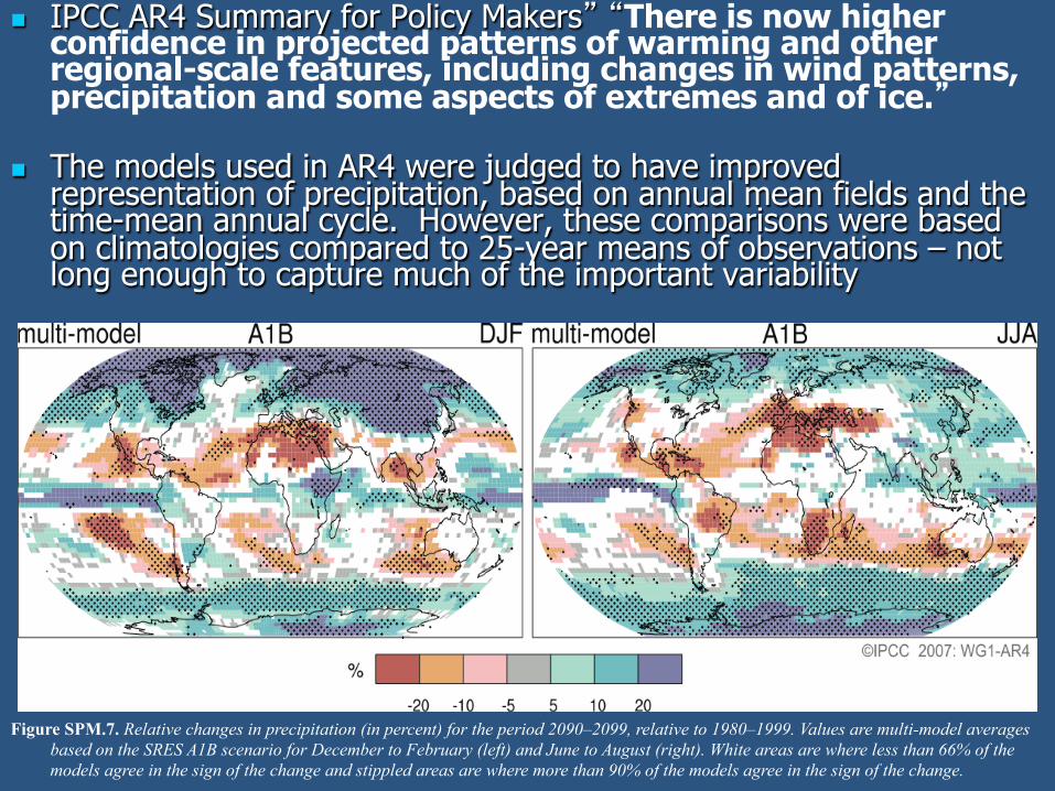
n  IPCC AR4 Summary for Policy Makers” “There is now higher confidence in projected patterns of warming and other regional-scale features, including changes in wind patterns, precipitation and some aspects of extremes and of ice.”

n  The models used in AR4 were judged to have improved representation of precipitation, based on annual mean fields and the time-mean annual cycle. However, these comparisons were based on climatologies compared to 25-year means of observations – not long enough to capture much of the important variability

Figure SPM.7. Relative changes in precipitation (in percent) for the period 2090–2099, relative to 1980–1999. Values are multi-model averages based on the SRES A1B scenario for December to February (left) and June to August (right). White areas are where less than 66% of the models agree in the sign of the change and stippled areas are where more than 90% of the models agree in the sign of the change.

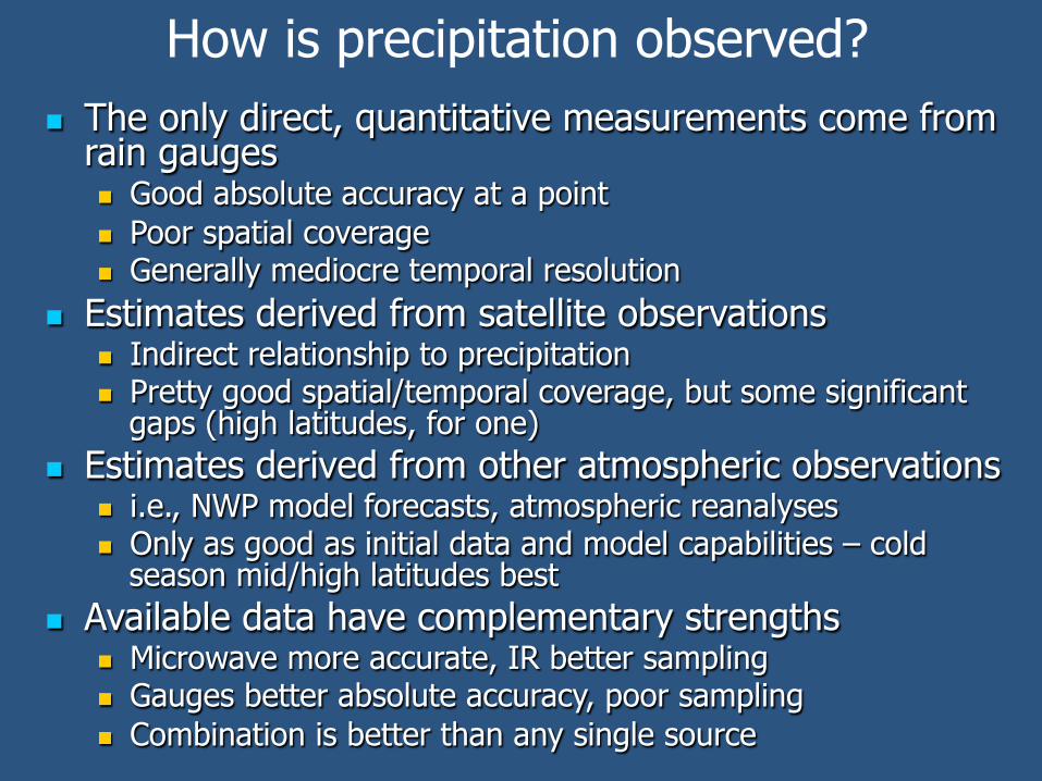
How is precipitation observed? n  The only direct, quantitative measurements come from

rain gauges n  Good absolute accuracy at a point n  Poor spatial coverage n  Generally mediocre temporal resolution

n  Estimates derived from satellite observations n  Indirect relationship to precipitation n  Pretty good spatial/temporal coverage, but some significant

gaps (high latitudes, for one) n  Estimates derived from other atmospheric observations

n  i.e., NWP model forecasts, atmospheric reanalyses n  Only as good as initial data and model capabilities – cold

season mid/high latitudes best n  Available data have complementary strengths

n  Microwave more accurate, IR better sampling n  Gauges better absolute accuracy, poor sampling n  Combination is better than any single source

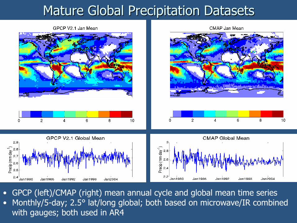
Mature Global Precipitation Datasets

•  GPCP (left)/CMAP (right) mean annual cycle and global mean time series •  Monthly/5-day; 2.5° lat/long global; both based on microwave/IR combined

with gauges; both used in AR4

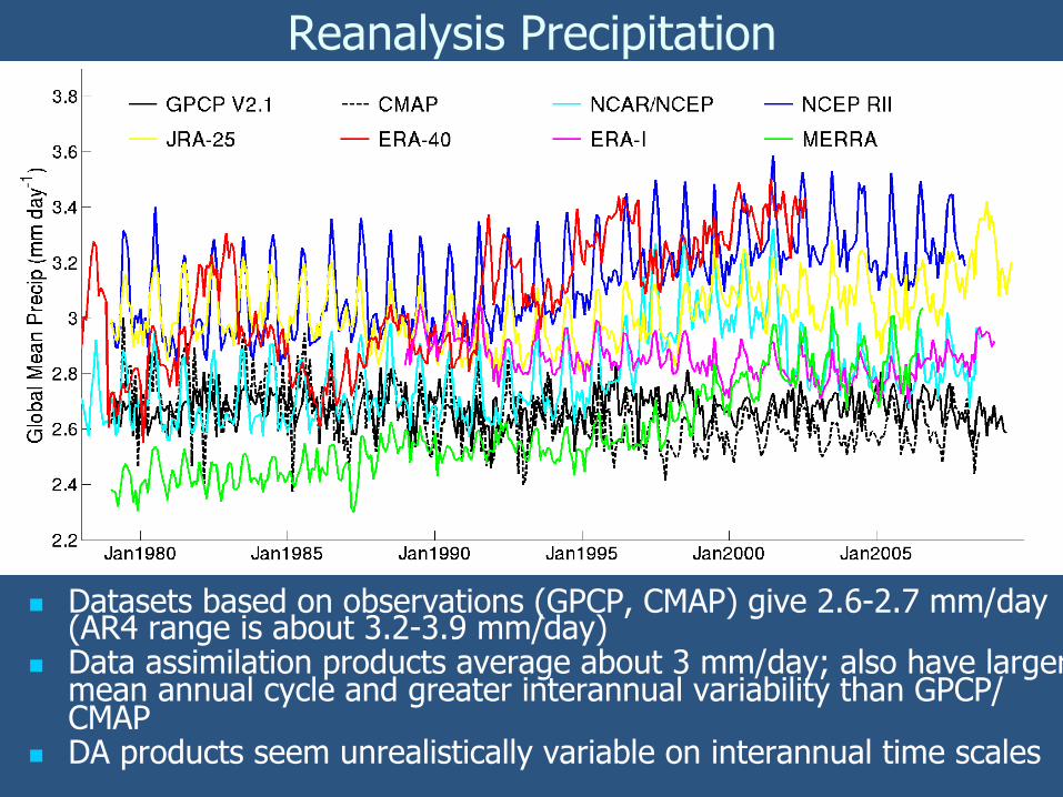
n  Datasets based on observations (GPCP, CMAP) give 2.6-2.7 mm/day (AR4 range is about 3.2-3.9 mm/day)

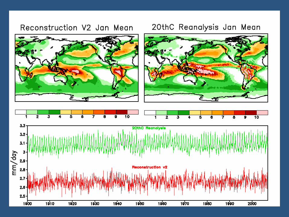
n  Data assimilation products average about 3 mm/day; also have larger mean annual cycle and greater interannual variability than GPCP/CMAP

n  DA products seem unrealistically variable on interannual time scales

Reanalysis Precipitation

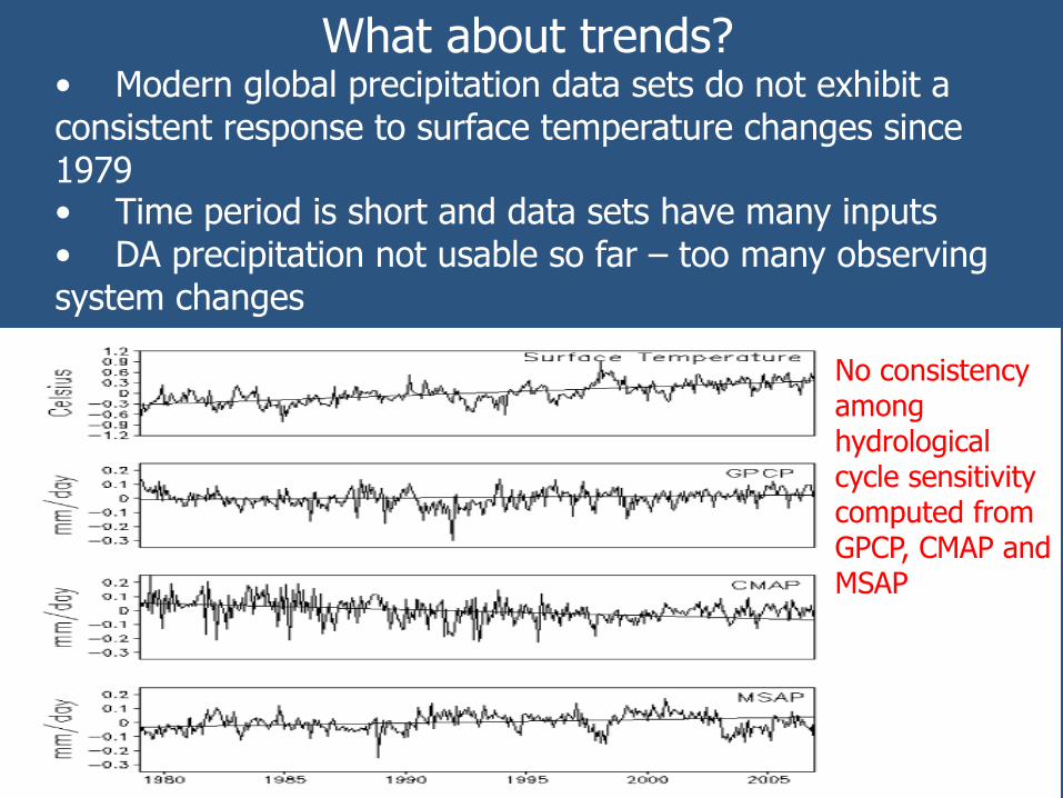
No consistency among hydrological cycle sensitivity computed from GPCP, CMAP and MSAP

What about trends? •  Modern global precipitation data sets do not exhibit a consistent response to surface temperature changes since 1979 •  Time period is short and data sets have many inputs •  DA precipitation not usable so far – too many observing system changes

n  Global Averages – reanalyses have higher global precipitation than observations n  GPCP and CMAP have potential systematic errors that could

contribute to this difference: n  Orographic and high latitude precipitation is very poorly

observed n  There is some evidence that the passive microwave estimates

may be biased low over tropical oceans n  Annual Cycle – GPCP and CMAP disagree on the (very

small) annual cycle of global mean precipitation, but are generally consistent with the spatial details of the seasonal cycle n  reanalyses generally exhibit higher values during Northern

Hemisphere summer; simulations not as consistent n  Observed data sets have pronounced hemispheric and land/

ocean annual cycles that almost exactly compensate – a potential test for model simulations

n  Trends – no consistent signal in modern datasets n  Modes of Variability – Quite good for seasonal to

interannual scales, ENSO in particular (not discussed)

Reconstruction of Near-Global Precipitation Variations Back to 1900 Based on Gauges and Correlations with SST and SLP

(see Tom Smith for hard questions)

n  Base Satellite Data n  Need global satellite analyses to establish statistics n  GPCP, CMAP and MSAP tested; GPCP works best

n  Direct Reconstructions: fitting data to Empirical Orthogonal Functions – Primary Source n  Global EOF (or PC) analysis of GPCP annual anomalies – 10 modes n  Fit annual gauge-station data to these modes n  Compute residual monthly modes using GPCP data – 40 modes n  Fit residuals of monthly gauge data to these modes n  Yields time series of monthly anomalies on 5° grid 1900-2008 n  This preserves multi-decadal signal

n  Indirect Reconstructions: using Canonical Correlation Analysis – (Nearly) Independent Check n  Correlate fields of sea-surface temperature (SST) and sea-level pressure

(SLP) with fields of precipitation during satellite era n  Both SST and SLP analyzed for the 20th century; annual anomalies

n  Global Averages – we can compare AR4 model simulations and the NOAA/ESRL 20th Century reanalysis against the reconstructions (where the mean is strongly influenced by GPCP)

n  Annual Cycle – reconstruction annual cycle can be compared against 20th Century reanalysis

n  Long-term Variability – 100+ years should be enough to compare trends and decadal variations

n  Modes of Variability – how well do reconstructions and reanalysis represent ENSO, NAO, etc.?

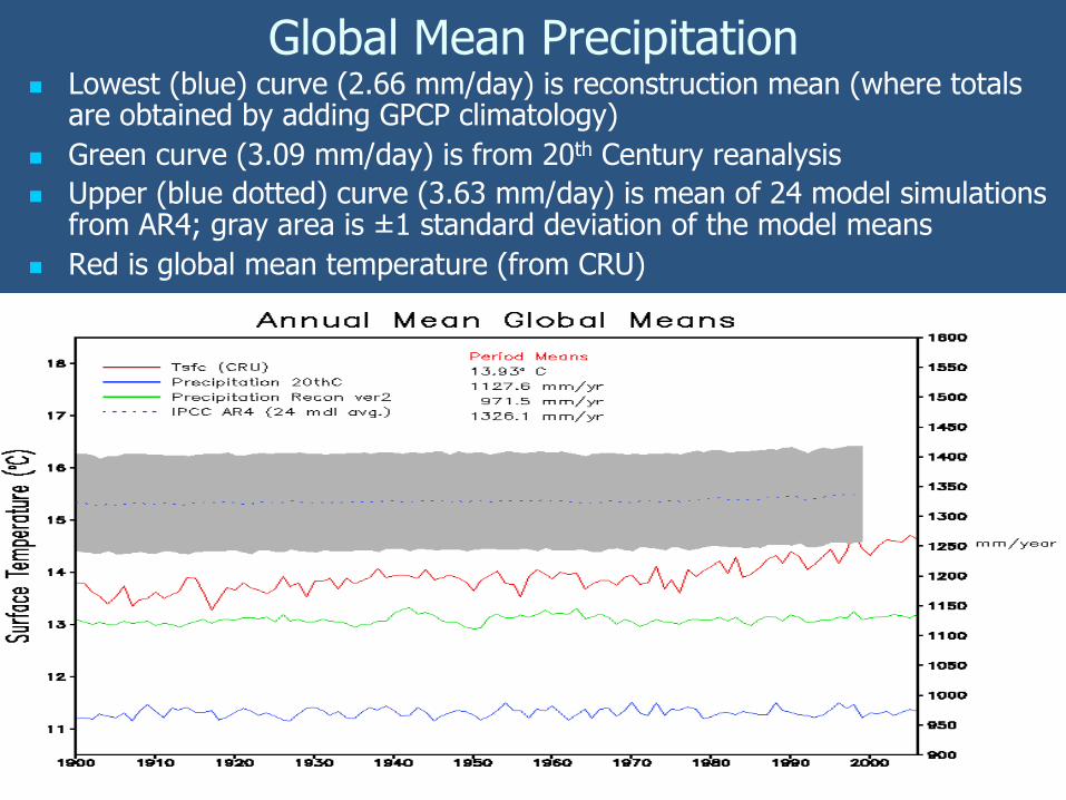
Global Mean Precipitation n  Lowest (blue) curve (2.66 mm/day) is reconstruction mean (where totals

are obtained by adding GPCP climatology) n  Green curve (3.09 mm/day) is from 20th Century reanalysis n  Upper (blue dotted) curve (3.63 mm/day) is mean of 24 model simulations

from AR4; gray area is ±1 standard deviation of the model means n  Red is global mean temperature (from CRU)

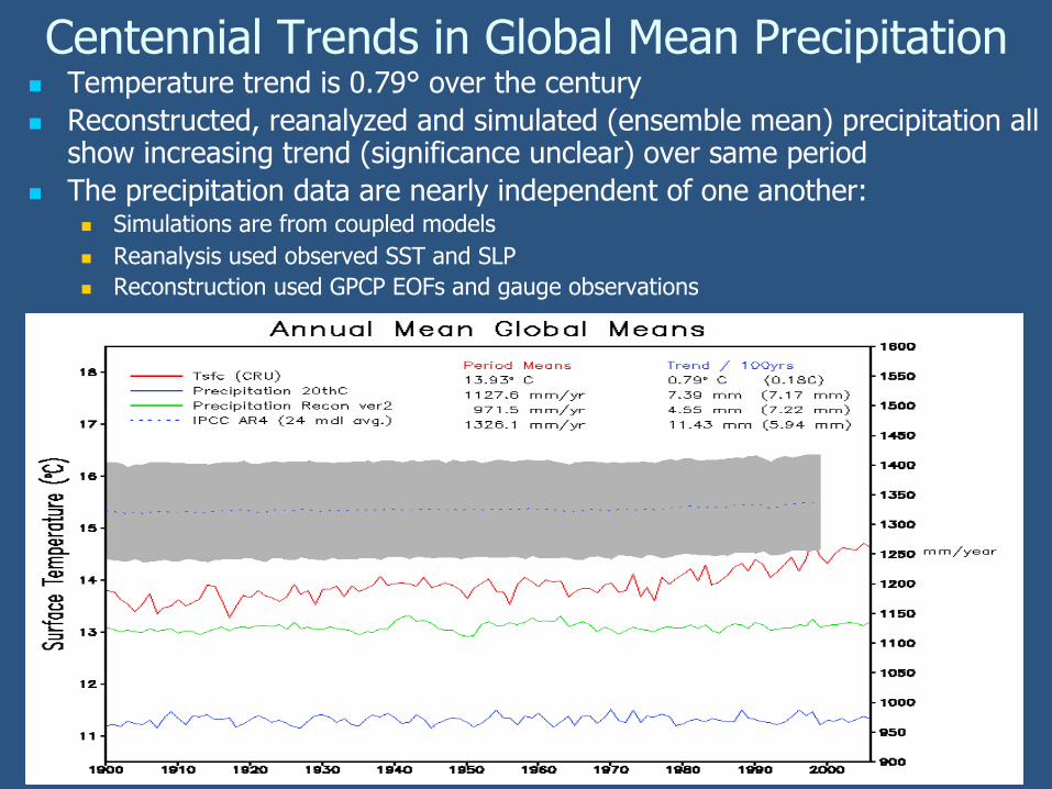
Centennial Trends in Global Mean Precipitation n  Temperature trend is 0.79° over the century n  Reconstructed, reanalyzed and simulated (ensemble mean) precipitation all

show increasing trend (significance unclear) over same period n  The precipitation data are nearly independent of one another:

n  Simulations are from coupled models n  Reanalysis used observed SST and SLP n  Reconstruction used GPCP EOFs and gauge observations

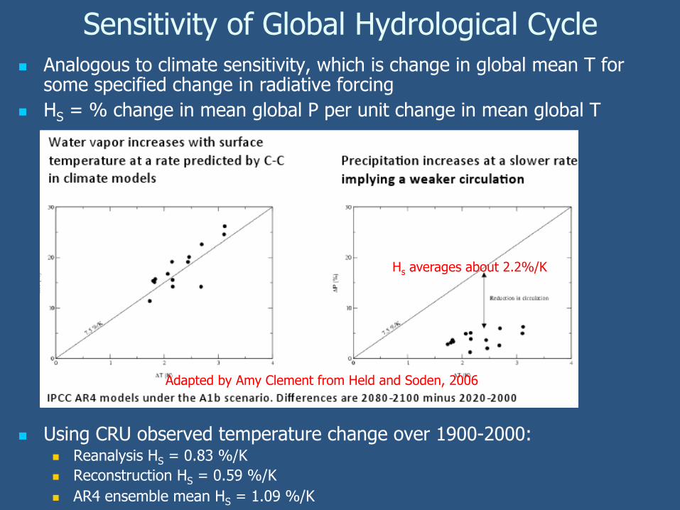
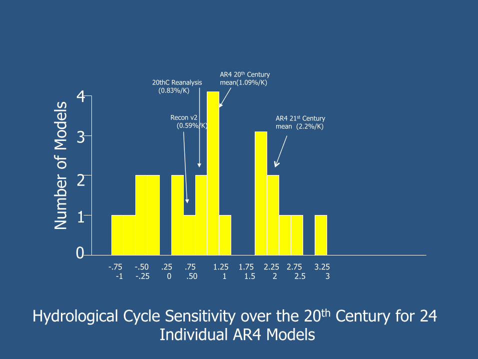
Sensitivity of Global Hydrological Cycle n  Analogous to climate sensitivity, which is change in global mean T for

some specified change in radiative forcing

n  HS = % change in mean global P per unit change in mean global T

n  Using CRU observed temperature change over 1900-2000: n  Reanalysis HS = 0.83 %/K n  Reconstruction HS = 0.59 %/K n  AR4 ensemble mean HS = 1.09 %/K

Adapted by Amy Clement from Held and Soden, 2006

Hs averages about 2.2%/K

0

1

4

-.75 -.50 .25 .75 1.25 1.75 2.25 2.75 3.25 -1 -.25 0 .50 1 1.5 2 2.5 3

Hydrological Cycle Sensitivity over the 20th Century for 24 Individual AR4 Models

AR4 20th Century mean(1.09%/K) 20thC Reanalysis

(0.83%/K)

Recon v2 (0.59%/K)

Num

ber

of M

odel

s

2

3 AR4 21st Century mean (2.2%/K)

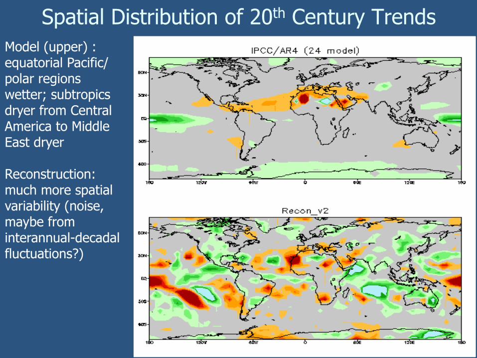
Model (upper) : equatorial Pacific/polar regions wetter; subtropics dryer from Central America to Middle East dryer Reconstruction: much more spatial variability (noise, maybe from interannual-decadal fluctuations?)

Spatial Distribution of 20th Century Trends

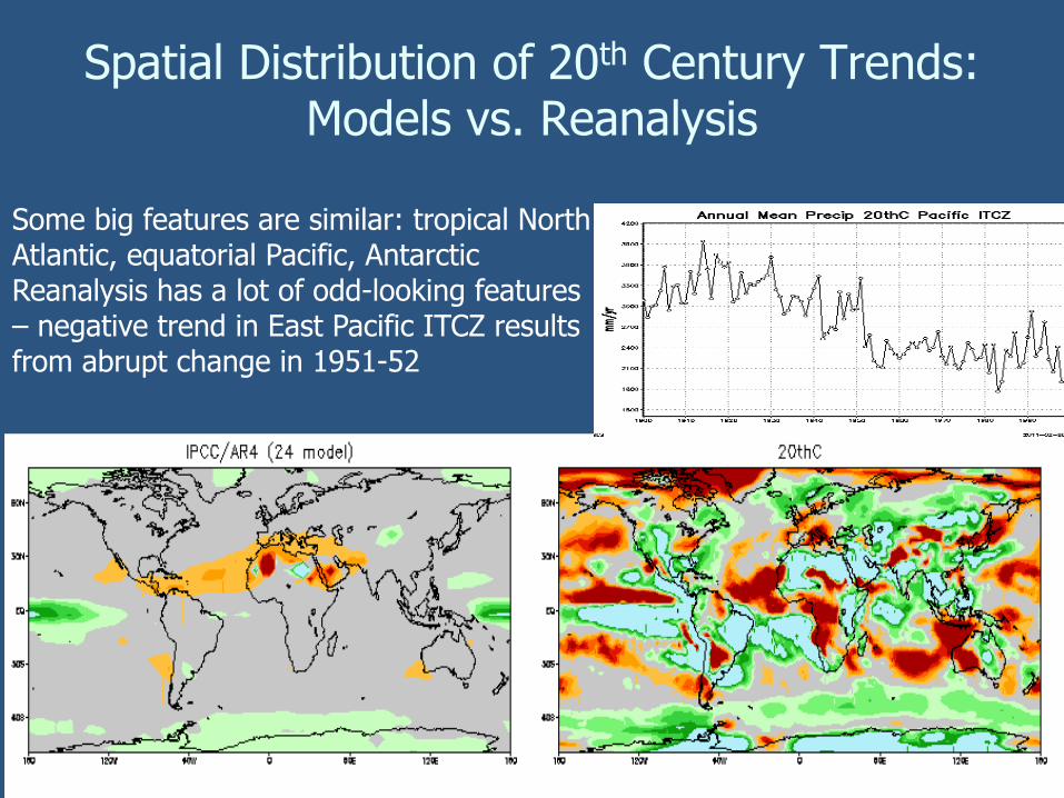
Some big features are similar: tropical North Atlantic, equatorial Pacific, Antarctic Reanalysis has a lot of odd-looking features – negative trend in East Pacific ITCZ results from abrupt change in 1951-52

Spatial Distribution of 20th Century Trends: Models vs. Reanalysis

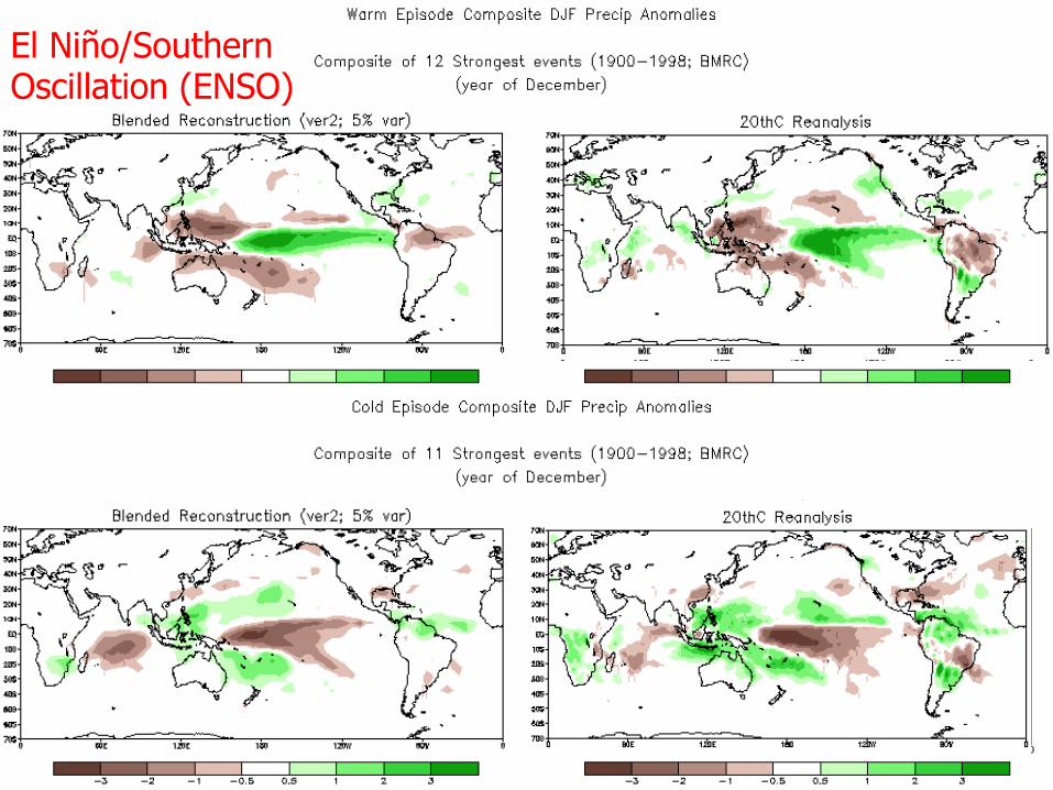
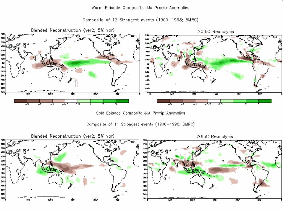
n  Modes of Variability – in examining temperature, precipitation and circulation data, climate scientists have identified a number of coherent phenomena that have consistent patterns of behavior that cover large parts of the world and last for extended periods of time n  ENSO, NAO, AO/AAO, etc.

n  The goal here is to compare the ability of reconstructions and reanalyses to resolve these signals in global precipitation

X X X X X X X X X X X

El Niño/Southern Oscillation (ENSO)

20th Century Reanalysis

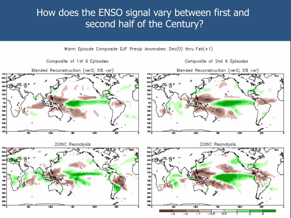
How does the ENSO signal vary between first and second half of the Century?

20th Century Reanalysis

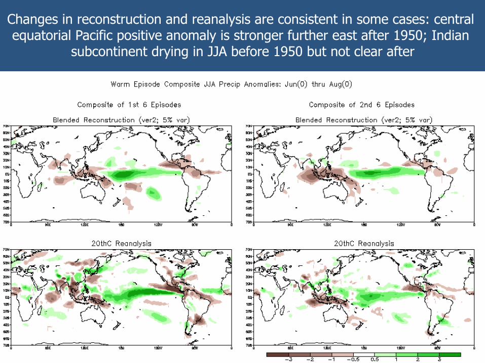
Changes in reconstruction and reanalysis are consistent in some cases: central equatorial Pacific positive anomaly is stronger further east after 1950; Indian

subcontinent drying in JJA before 1950 but not clear after

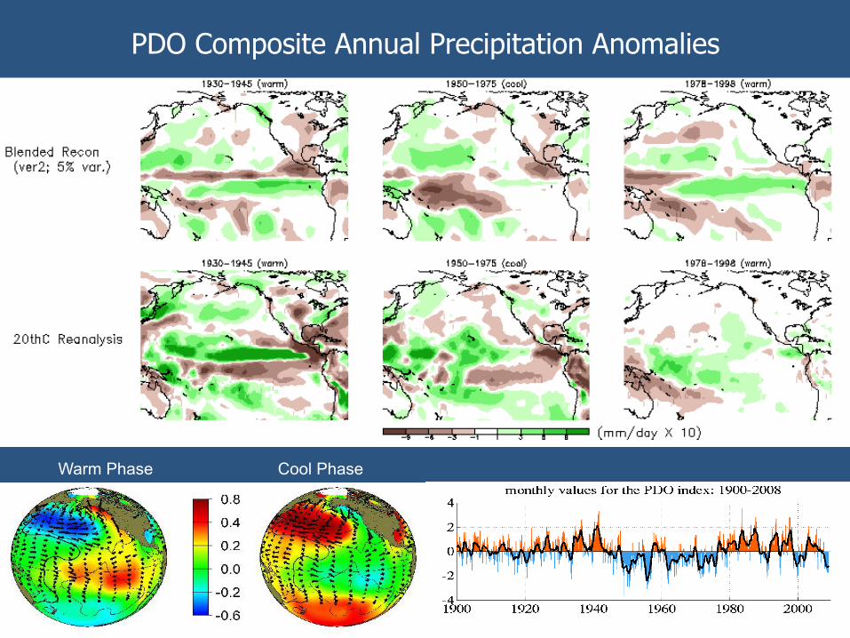
PDO Composite Annual Precipitation Anomalies

Warm Phase Cool Phase

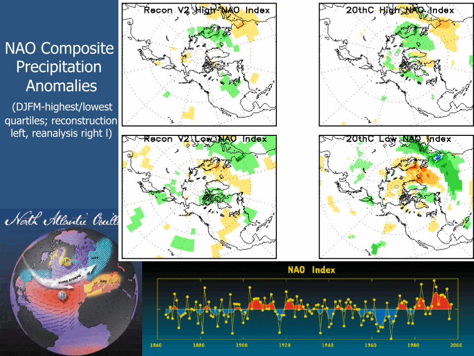
NAO Composite Precipitation Anomalies

(DJFM-highest/lowest quartiles; reconstruction left, reanalysis right l)

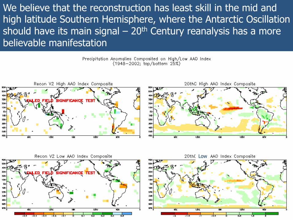
We believe that the reconstruction has least skill in the mid and high latitude Southern Hemisphere, where the Antarctic Oscillation should have its main signal – 20th Century reanalysis has a more believable manifestation

Low

27

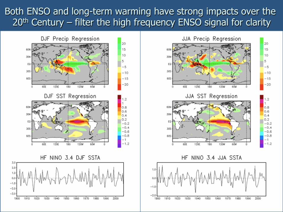
Both ENSO and long-term warming have strong impacts over the 20th Century – filter the high frequency ENSO signal for clarity

n  Remove the high frequency ENSO signal

n  Examine the remaining variance: n  Oceanic variations

often associated with strong SST changes

n  Increases: Tropical Indian, along SPCZ, Tropical N. Atlantic, Arctic

28

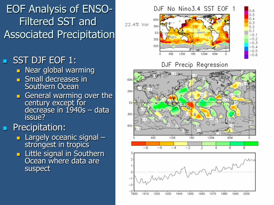
EOF Analysis of ENSO-Filtered SST and

Associated Precipitation

n  SST DJF EOF 1: n  Near global warming n  Small decreases in

Southern Ocean n  General warming over the

century except for decrease in 1940s – data issue?

n  Precipitation: n  Largely oceanic signal –

strongest in tropics n  Little signal in Southern

Ocean where data are suspect

29

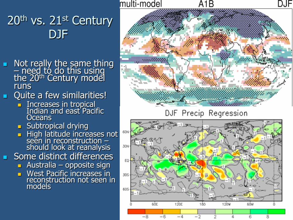
20th vs. 21st Century DJF

n  Not really the same thing – need to do this using the 20th Century model runs

n  Quite a few similarities! n  Increases in tropical

Indian and east Pacific Oceans

n  Subtropical drying n  High latitude increases not

seen in reconstruction – should look at reanalysis

n  Some distinct differences n  Australia – opposite sign n  West Pacific increases in

reconstruction not seen in models

30

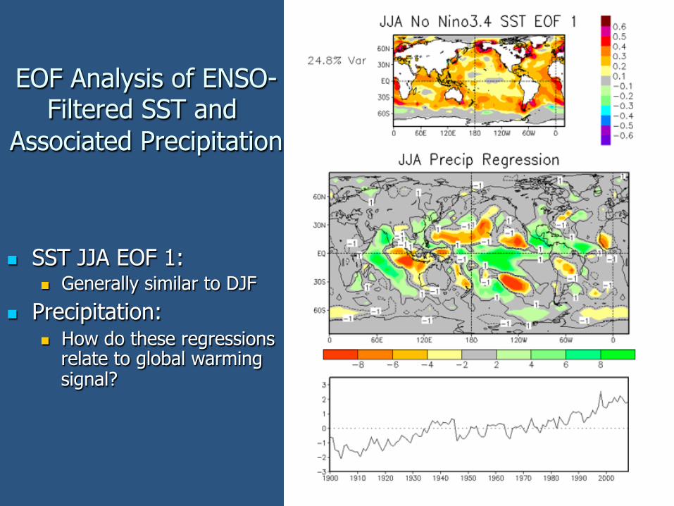
EOF Analysis of ENSO-Filtered SST and

Associated Precipitation

n  SST JJA EOF 1: n  Generally similar to DJF

n  Precipitation: n  How do these regressions

relate to global warming signal?

31

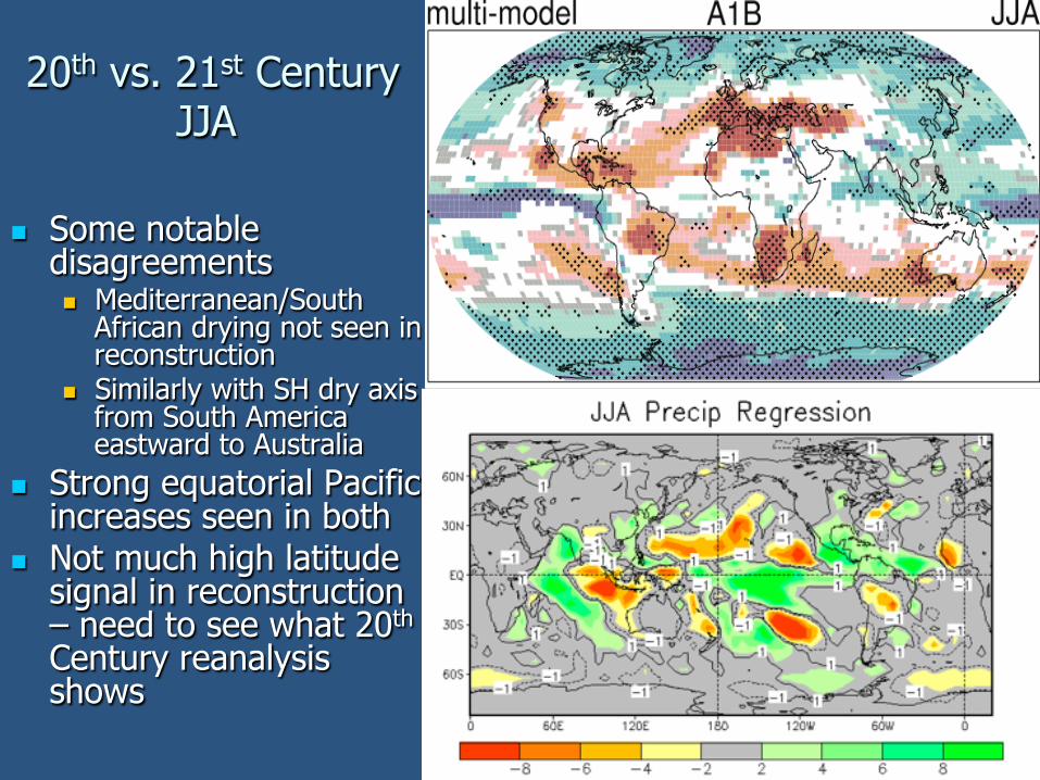
20th vs. 21st Century JJA

n  Some notable disagreements n  Mediterranean/South

African drying not seen in reconstruction

n  Similarly with SH dry axis from South America eastward to Australia

n  Strong equatorial Pacific increases seen in both

n  Not much high latitude signal in reconstruction – need to see what 20th Century reanalysis shows

n  Global Averages – wide disparity among the available sources n  Reconstruction is lowest, simulations are highest, reanalysis in

between n  3.1 mm/day +/- 20% n  None of the specific values is particularly believable

n  Annual Cycle – Given the highly asymmetric distribution of land/ocean between the hemispheres, a small annual cycle in global mean precipitation is not unreasonable n  20th Century reanalysis ranges from 3-3.2 mm/day; reconstruction,

based on GPCP, exhibits similar range of variability but not as clearly tied to the seasonal cycle

n  Trends – reconstruction, reanalysis and ensemble mean of AR4 simulations all exhibit positive trend n  All three give hydrological cycle sensitivity (for 20th Century)

lower than AR4 projections; greater than 0; within range of model suite

n  Some similarity in patterns among models, reconstruction, reanalysis

n  Modes of Variability – Both reanalysis and reconstruction appear to capture main signals n  Might be possible to create a combined product that is superior to

either alone n  Didn’t try to evaluate models

Conclusions n  Validating model simulations/hindcasts against observed

precipitation crucial to enhance confidence in predictions/projections n  Better “observations” necessary – still not certain what is really

happening n  Standard protocol/set of metrics desirable

n  “Modern” precipitation data sets (GPCP, CMAP) still useful n  Shortcomings remain – resolution, estimates of uncertainty n  Development continues

n  20th Century precipitation reconstruction and reanalysis available n  Different methods give sufficiently similar results to indicate some

validity n  Useful for testing global models